Toward a formal theory for computing machines made out of whatever physics offers: extended version

Abstract

Approaching limitations of digital computing technologies have spurred research in neuromorphic and other unconventional approaches to computing. Here we argue that if we want to systematically engineer computing systems that are based on unconventional physical effects, we need guidance from a formal theory that is different from the symbolic-algorithmic theory of today’s computer science textbooks. We propose a general strategy for developing such a theory, and within that general view, a specific approach that we call fluent computing. In contrast to Turing, who modeled computing processes from a top-down perspective as symbolic reasoning, we adopt the scientific paradigm of physics and model physical computing systems bottom-up by formalizing what can ultimately be measured in any physical substrate. This leads to an understanding of computing as the structuring of processes, while classical models of computing systems describe the processing of structures.

This is a greatly extended version of a perspective article H. Jaeger . (2023) that appeared in Nature Communications.

1 Introduction

The all-overturning powers of digital computing (DC) technologies need no elaboration. Since a decade or so it has however becoming increasingly clear that DC technologies are accelerating into a narrowing lane with regards to energy footprint Andrae  Edler (2015); toxic waste Zhao . (2019); physical, technological and economical limits of miniaturization Waldrop (2016) and vulnerabilites of ever growing software complexity Ebert (2018). These conditions have spurred explorations of alternatives to digital computing. Currently the most widely and deeply explored non-digital route to computing is neuromorphic computing Mead (1990) — use biological brains as role model for energy-efficient and high-throughput parallel algorithms and novel kinds of microchips. We also see a reinvigorated study of other unconventional computing paradigms, of which there are many. They have been introduced under names like natural computing, in-materio computing (or in-materia computing Ricciardi  Milano (2022)), emergent computation, physical computing, reservoir computing European Commission Author Collective (2009); Adamatzky (2017); H. Jaeger (20211), and they search for computational exploits in a wide variety of biological, chemical and physical systems and substrates. Examples are analog electronic computers Bournez  Pouly (2021), slime moulds Adamatzky (2018), physical reservoir systems Tanaka . (2019), DNA reactors van Noort . (2002); Doty (2012), chemical reaction networks Monti . (2017), ant colonies Dorigo  Gambardella (1997), or social decision making networks M. Minsky (1986); McPhail . (1992). Some of these initiatives can look back on a long history.

Today a large variety of systems are being investigated in the wide fields of neuromorphic and other unconventional computing researches. These systems are artifical or natural, exist as formal models, digital simulations, manufactured hardware, or are identified in natural hosts like DNA soups, immune systems, cells, brains or animal societies. All of these systems ’compute’ or “process information” in one way or another. They serve different purposes like signal processing and control, creative problem solving, optimization, autonomous decision-making and agent intelligence. Their behaviour can be shaped (or not) by users according to various pardigms, including programming, system hardware configuration, training, evolutionary optimization, or self-organized task adapation. Physical materials and devices offer a limitless reservoir of physical phenomena for building unconventional computing machines. In turn, these phenomena can be modeled by a likewise almost limitless range of mathematical constructs. Often these constructs are quite generic and can be found in almost every sufficiently complex physical or neural system — for instance oscillations, chaos and other attractor-like phenomena; hysteresis; many sorts of bifurcations and input-induced transits between basins of attraction; spatiotemporal pattern formation; intrinsic noise; phase transitions. The pertinent literature for each of them is so extensive and diverse that it defies a systematic survey. Other mathematical constructs are more specific, for instance heteroclinic channels and attractor relics Rabinovich . (2008); Gros (2009), self-organized criticality Chialvo (2010); Stieg . (2012); Beggs  Timme (2012) or solitons and waves Lins  Schöner (2014); Grollier . (2020).

Across the diversity of materials, methods and motives we perceive a growing awareness (or wish) that there is (or should be) a common ground from which these diverse branches of research arise, and in which they can (or might) become re-united — a unified science of information processing systems which is more general than, or just different from, today’s canonical science of symbolic-discrete computing. While this is a vague and distant goal, the relevant communities are making increasingly energetic efforts to move closer together, such that they can learn from each other. This is witnessed by high-profile target articles Schuman . (2022); Mehonic  Kenyon (2022), interdisciplinary collection volumes Adamatzky (2017), conferences and workshops, large-scale public-funded research projects (some in the acknowledgements at the end of this article), or newly founded academic study programs and research institutes (some are listed by MehonicKenyon22).

At present, most of these activities label themselves as ’neuromorphic’. We see several reasons for the current prominence of the ’neuromorphic’ paradigm: the blazing achievements of deep neural networks in machine learning; concrete technological promises of memristive synapses for in-memory computing; and the unique standing of brains as the role model which, among all natural ’computing’ systems, is the most complex, powerful and intriguing one.

We do not want to separate neuromorphic from other unconventional approaches to ’computing’. Both lines of study can be seen as belonging together in that they are interested in ’natural’ aspects of computing systems like self-organization, adaptability, learning, creativity, energy efficiency, noise robustness, error tolerance and graceful degradation, autonomy, continuous-time interaction with an environment, or statistical dynamics in large ensembles — all of these are not natively connected with the digital-symbolic computing paradigm.

To preclude misunderstandings we mention that we consider quantum computing in its classical form — carefully stabilized qbit carriers exploiting quantum state superposition for parallel search — as a variant of classical symbolic computing rather than as an example of unconventional computing. The theory and intended applications of traditional quantum computing are couched in the classical Turing paradigm, offering faster algorithmic solutions for tasks that could likewise be solved by Turing machines.

Progress in neuromorphic and other unconventional computing is slow. While a wealth of ideas, methods, materials, devices, proof-of-principle demonstrators, and analyses are being generated, these results remain largely separated by disciplinary boundaries despite all efforts for community-building. We believe that this state of affairs will persist as long as there is no unifying formal theory that could connect the dots. Such a formal theory would be crucial for a scientific discipline of engineering neuromorphic and other unconventional computing systems in a principled, systematic way. We are certainly not the only ones to deplore the absence of such a foundation in a unifying theory: “The ultimate goal would be a unified domain of all forms of computation, in as far as is possible…” European Commission Author Collective (2009); “As the domain of computer science grows, as one computational model no longer fits all, its true nature is being revealed… New computers could inform new computational theories, and those theories could then help us understand the physical world around us” D. Horsman . (2017); “there is still a gap in defining abstractions for using neuromorphic computers more broadly” Schuman . (2022); “The neuromorphic community … lacks a focus. […] We need holistic and concurrent design across the whole stack […] to ensure as full an integration of bio-inspired principles into hardware as possible” Mehonic  Kenyon (2022).

There already exists a broad spectrum of formal theories that may be candidates or starting points for a unified theory of neuromorphic and unconventional computing systems. These theories have been developed in computer science, theoretical natural sciences, systems engineering and complex systems research for a variety of goals: to enable an interpretation of natural processes as ’computing’; to unify the laws of physics in a concept of ’information’; to help describing and understanding neural and cognitive processes; to describe complex engineered or natural systems through conceptual and/or procedural hierarchies; or to guide the design of computing machines other than digital-symbolic ones. We highlight the range of existing formal frameworks by listing some of them — to underline the confusing wealth and diversity of our findings, we do this in random order:

• The classical models of analog computing systems formalize analog mechanical or electronic devices that realize real-valued elementary operations like addition or integration can be combined in complex system for realizing a hierarchy of real-valued functions. These hierarchies had originally been shaped in the molds of symbolic-logical theories of Turing-computable functions Shannon (1941); Moore (1996), but later the perspective has broadened a lot (surveyed by BournezPouly21).

• A traditional subfield of AI, qualitative physics, Forbus (1988) (closely related: naive physics, qualitative reasoning) explores logic-based formalisms which capture the everyday reasoning of humans about their mesoscale physical environment.

• Ulf Grenander’s pattern theory, especially in the transparent workout of David Mumford Mumford (1994), offers a thoroughly formal account of how (primarily spatial / visual) “patterns” can be generated, compounded, transformed and encoded. Pattern theory is sophisticated — David Mumford is a recipient of the Fields Medal, and he considers pattern theory a candidate for “a mathematical theory underlying intelligence” Mumford (2002).

• Insights gained in the fields of emergent computation Forrest (1990) steer attention to the powers of collective phenomena in dissipative systems, where macrolevel phenomena “self-organize” from the interactions of microlevel components.

• Complex systems modeling general. Formal models of complex natural systems are regularly chiseled out in formats that have structural and procedural similarities with formalisms in AI or computer science. Such models admit interpretations of structures and processes in ’computational’ or ’cognitive’ or ’information processing’ terms. A survey cannot be attempted. An example are models in motion science, which capture bodily motion patterns of animals and humans. Important work in this field views complex, continuous physical motion patterns in ways that have strong analogies with cognitive and computational processes, by defining criteria for segmenting and composing bodily motions hierarchically in multiple spatial and temporal scales, modeling their planning and execution control, and analysing how they can be semantically interpreted by observers Hogan  Flash (1987); Thoroughman  Shadmehr (2000); Roether . (2010); Land . (2013).

• The theory of autopoeitic systems, established by Humberto Maturana and Francisco J. Varela Varela . (1974); Maturana  Varela (1984), explains the stability of biological organisms through internal feedback loops in which all parts and functions engage in a concert to reproduce themselves. In this light, cognitive processes are not seen as based on representations of external reality, but as constituting their own inner reality in network of interconnected processes. This view challenges commonsense and philosophical conceptions of cognitive representations, exerting a lasting impact outside theoretical biology in epistemology, cognitive science, sociology and other fields Razeto-Barry (2012). Principles from autopoeisis have frequently been invoked by proponents of behavior-based robotics Brooks (1995) and ’new AI’ Pfeifer  Scheier (1999) to explain how intelligent information processing does not need explicit internal representations (in the classical AI spirit) of an agent’s environment.

• Stream automata Endrullis . (2019) aim at extending the classical theory of finite-state automata to infinite data stream processing. This can be seen as a step toward modeling neural processing with tools that grow out of classical computer science, because brains (and other natural systems that have been regarded as processing information) are also stream processing systems.

• Process calculi and other mathematical models, including the well-known Petri nets Petri  Reisig (2008), aim at modeling distributed information processing which unfolds in concurrent subprocesses. These formalisms belong to classical computer science. A category-theoretical unification is proposed by WinskelNielsen93. These modeling tools have been adapted outside computer science to model processing of information or materials in other engineered or natural systems, notably by Luca Cardelli who tailored these tools in many ways to formalize processes in biological and chemical systems (example: membrane computing Cardelli (2005); Paun (2010)).

• Interactive symbolic computing. In some non-standard use-cases considered in modern computer science, ’computing’ is seen as an interaction sequence between a (otherwise classical symbolic-discrete) computer and a user. The information feedback through the user extends the class of problems that can be solved by such interaction pairs beyond the Turing-computable problems Wegner  Goldin (2003).

• In computer science and systems engineering, hybrid systems are systems that combine computational and physical processing, or software and hardware, or discrete and continuous states. Formalisms for modeling such systems are likewise hybrids of classical discrete-symbolic models of computer science (often automata models) with continuous-state physical modeling inserts Lynch . (2003); Geuvers . (2010).

• Complexity theory for neural networks. KwisthoutDonselaar20 consider Turing machines, which upon presentation of a task input automatically construct a formal model of a spiking neural network that can process this task, and investigates the combined consumption of computational resources for such twin systems. For the neural network model he allows unconventional resource categories like the number of used spikes. This work renders spiking neural networks accessible to classical theory of computational complexity, but does not specify how the neural networks spawned by the Turing machine are concretely designed, and the approach is only applicable to a specific formal model of neural networks, not to general physical computing systems.

• Recurrent neural networks (RNNs) are neural networks whose cyclic connection topology makes them dynamical systems. Always present since the beginnings of the study of neural networks McCulloch  Pitts (1943), this family of models has risen to new levels of importance through their wide use in deep learning. Very recently there even seems to be a new surge of interest because innovative RNN architectures have become at least competitive with, and sometimes superior to transformer networks, which at present are deemed the most powerful deep learning systems Zucchet . (2023). The family of RNN models at large is so diverse that we cannot attempt to discuss them here in fuller scope.

• Reservoir computing is a special RNN design for supervised learning that originated in machine learning H. Jaeger (2001) and computational neuroscience Maass . (2002). A randomly connected recurrent neural network is excited by an input signal, and from the richly varied nonlinear response signals inside the ’reservoir’ network a trainable output signal is linearly combined. This sort of system has been thoroughly investigated by mathematicians, revealing which input-output signal transformations can be realized Grigoryeva  Ortega (20182) — namely the class of fading memory tasks. We mention reservoir computing here separately from RNNs in general because reservoir systems have become variously adopted by materials scientists, who replace the neural reservoir by nonlinearly excitable physical substrates Tanaka . (2019).

• The Neural Engineering Framework Stewart . (2011), originally developed by Chris Eliasmith and Charles Anderson and used in a sizeable community of cognitive neuroscientists Bekolay . (2014); Eliasmith . (2012); Neckar . (2019); Taatgen (2019); Angelidis . (2021), provides mathematical analyses and design rules for interacting modules of spiking neural networks that realize signal processing filters, which are specified by ordinary differential equations.

• Cognitive information processing as statistical inference. Intelligent agents that operate in stochastic environments must be able to compute probability distributions of the expected consequences of their actions. This core idea of a predictive brain Clark (2013) has been formally worked out in numerous formats and communities. The mechanical operations needed to reason with and about probability distributions are often realized through stochastic sampling dynamics H. Jaeger (20212). Some examples of workouts in this spirit:

  • The free energy principle of Friston (2010) casts the learning and adaptation of autonomous agents in challenging environments in a mathematical formalism that originated in statistical physics, information theory and Bayesian statistics. Specifically, the efforts of the learner, who needs to distil a useful representation of the results of its actions in a stochastic environment, is interpreted in terms of minimizing a quantity that is formally analogue to free energy in statistical physics. The high abstraction level of this mathematical framework admits a unified view on a variety of existing models of cognitive functions, representations, and learning, which are stated on behavioral, cognitive, or physiological levels.

  • Hopfield networks Hopfield (1982), Boltzmann machines Ackley . (1985) and the restricted Boltzmann machine Hinton  Salakuthdinov (2006) are classical instances of calling upon methods of statistical physics (in particular the Boltzmann distribution) for stochastic neural network models. A unifying review is given by MarulloAgliari20.

  • In machine learning outside neural networks, Bayesian networks Pearl  Russell (2003), dynamic Bayesian networks Murphy (2002), and most generally graphical models Jordan (2004) establish a unifying formal framework for representing and learning high-dimensional probability distributions and calculating inferences on them. Pecevskietal11 describe how statistical inferences in graphical models can be realized in stochastic spiking neural networks. While one standardly considers only inferences of conditional and marginal distributions, novel methods for identifying causal interactions between observables are claimed to have the potential to revolutionize machine learning because these methods may dramatically reduce the amount of training data needed to achieve a desired functionality Schölkopf . (2021).

• Connectionism refers to a hybrid symbolic-dynamical way of thinking about neural networks, which has been understood differently at different times. Here we point out spreading activation models of cognitive neural processing. These models are structured as graphs whose nodes are labeled with concept or operator names, with activating or inhibiting links between them. These formalisms are a crossover between symbolic AI (because of the symbolic node labels) and the parallel distributed neural processing paradigm (due to the continuous-time activation-based interaction). A deeply worked-out, exemplary family of connectionist models are the SHRUTI models of linguistic processing, which are “neurally motivated models of relational knowledge representation and rapid inference using temporal synchrony” Shastri (1999).

• Program engineering for spiking neurochips. Zhangetal20 present a method for engineering brain-inspired computing systems, programming them in a high-level formal design language, which is compiled down through an intermediate formalism to a machine interface level, which then can be mapped to the current most performant (digital) neuromorphic microprocessors. This approach is motivated by practical system engineering goals and in many ways follows the role model of AC compilation hierarchies. It is however limited to exactly the three specific modeling levels specified in this work, with different principles used for the respective encodings, and at the bottom end exclusively targets digitally programmable spiking neurochips.

• The Realtime Control System Albus (1993) of James Albus is a design scheme for control architectures of autonomous robotic systems, from the sensor-motor interface level to high-level knowledge-based planning and decision making. Like other models of modular cognitive architectures Samsonovich (2010), it is taken for granted that they are simulated on digital computers.

• In theoretical physics, [pan-]computationalism loosely refers to a variety of modeling approaches where formal concepts from symbolic computing or the Shannon concept of information are invoked to describe and explain the physical world (introduction: Zenil13a; examples: vonWeizsaecker85,Lloyd13,Wolfram20). A notably popular special format are cellular automata models, which capture self-organized pattern formation in physical substrates Zuse (1982); Wolfram (2002); Fredkin (2013).

• Physarum computing Adamatzky (2018) is a popular subject of experimental and theoretical studies in the unconventional computing arena. Physarum is a genus of slime molds, whose amazing life cycle comprises stadiums of single-cell amoeba-like organisms, merged macroscopic multi-nucleus megacells, and large multicell-bodies shaped as mycel webs or ’mushrooms’. Their individual and collective information-processing capabilities are investigated under biological aspects like orientation and navigation, but also under pure computational aspects — physarum colonies have been grown into Boolean circuits!

• Stochastic search for optimization tasks. Task-solving ’computing’ is variously framed as solving optimization tasks. When the cost landscapes are non-convex, complex and non-differentiable, stochastic search methods are the only known way to find good task solutions. A spectrum of ensemble-based parallel search methods has been proposed in various communities, for instance simulated annealing Kirkpatrick . (1983), (classical) DNA computing van Noort . (2002), or ant colony algorithms Dorigo  Gambardella (1997).

• Self-assembling DNA macromolecules Doty (2012) is a rather recent development in DNA computing. A mix of DNA-based nanomolecular complexes, each of which has a specific geometrical shape, is put into a reactor, in which these DNA ’tiles’ bind into growing complexes whose regular shapes encode and process symbolic information, akin to what happens in cellular automata or even a Turing machine. This model of information processing combines aspects of algorithmic processing, stochastic search, and self-organized pattern formation. This line of research is mostly carried out in computer simulations and abstract mathematical characterizations, with limited experimental demonstrations so far.

• In hyperdimensional computing Kanerva (2009), conceptually interpretable information items are represented by (long) random bitstrings, which can be transformed and combined by operations that correspond to logical or algebraic operations, and support the creation of hierarchically nested information structures. Hyperdimensional computing can be regarded as a version of stochastic computing, which goes back to vonNeumann56.

• Neural field theory Lins  Schöner (2014) formalizes neural dynamics in terms of spatiotemporal pattern formation on neural sheets. Moving neural ’solitons’ can represent the activation of concepts. The theory can give an integrative account of information processing of interacting top-down and bottom-up processing pathways across several layers in the neural hierarchy, and has been linked to the non-neural, generic machine learning architecture of map seeking circuits proposed by David Arathorn Gedeon  Arathorn (2007) — one of the very few formal models of bidirectional (top-down & bottom-up) information processing systems.

• Self-assembling DNA macromolecules Doty (2012) is a more recent development in DNA computing. A mix of DNA-based nanomolecular complexes, each of which has a specific geometrical shape, is put into a reactor, in which these DNA ’tiles’ bind into growing complexes whose regular shapes encode and process symbolic information, akin to what happens in cellular automata or even a Turing machine. This kind of information processing combines aspects of algorithmic processing, stochastic search, and self-organized pattern formation.This line of research is mostly carried out in computer simulations and abstract mathematical characterizations, with limited experimental demonstrations so far.

• Physarum computing Adamatzky (2018) is a popular subject of experimental and theoretical studies in the unconcenventional computing arena. Physarum is a genus of slime molds whose amazing life cycle comprises stadiums of single-cell amoeba-like organisms, merged macroscopic multi-nucleus megacells, and large multicell-bodies shaped as mycel webs or fructuation ’mushrooms’. Their individual and collective information-processing capabilities are investigated under biological aspects like orientation and navigation, but also under pure computational aspects — physarum organisms have been grown into Boolean circuits!

• Under the label of neural-symbolic integration or neural-symbolic computing, an interdiscipinary community with roots in formal logic, AI, cognitive science, and artificial neural networks has found together in a shared effort of interpreting neural dynamics in terms of logical information processing, and of designing hybrid neural-logical algorithms for learning and inference Besold . (2017). A broad range of formal models are proposed and discussed in this setting. This community is quite productive with founding a scientific association, book publications and a yearly workshop series.

This list is certainly incomplete. Still, it illustrates the already existing wealth of formally worked-out perspectives to interpret natural or engineered systems as ’computing’, ’information processing’, or ’cognitive’ in some way or other that differs from the standard model of digital/symbolic/algorithmic computing. Obviously, none of these approaches has yet established itself as a commonly agreed unifying theory framework for the entire community of neuromorphic and other unconventional computing investigators. This is inevitable when one considers the diversity of scientific or epistemological goals that gave rise to these efforts. In order to tie together the spreading-out threads of neuromorphic and other unconventional computing researches — and thus laying the foundations for a scientific engineering discipline — a unifying theory of ’computing’ arising from whatever physics can offer is needed. All of the currently available formal models of (wide-sense) computing systems are missing one or more of the following necessary conditions that such a unifying general formal theory of physical computing systems (GFT) theory must satisfy:

1. Phenomenal openness. A GFT must provide formal tools to express ’computational’ functionalities that emerge from a wide variety of physical phenomena. It is not enough for a GFT to address, exclusively, either multistable switching, or the stochastic dynamics of statistical ensemble systems, or self-organized pattern formation.

2. Interpretability. A GFT must include ways to formally characterize the use-cases and tasks that can be served by a given physical computing system. It is not enough for a GFT to capture the ’mechanics’ of computing systems — it must also give an account of what the mechanical processes ’mean’ - their task-related semantics.

3. Scalability. The range of possible tasks which can be addressed through GFT models must be very wide. It is not enough for a GFT to cover only, for example, supervised learning or stochastic search tasks. Furthermore, the complexity of achievable tasks must be arbitrarily scalable.

4. Model abstraction. A GFT must provide rigorous methods for model abstraction. For practical system engineering it is necessary to describe the workings of a computing system at different levels of granularity — fine-grained and hardware-oriented at low levels of abstraction, coarse-grained and task-oriented at higher abstraction levels.

The textbook theory of symbolic/digital computing excels with regards to points 2–4 but fails at 1. As far as we can see, the only approach to ’computing’ which to some extent fulfils condition 1 is reservoir computing, which explains its popularity in computational materials research — but reservoir computing has nothing to offer with regards to 2–4. Some other approaches from our listings can accommodate some but not all of our four requirements, but many fall short in all regards 1–4.

We have left out one interesting objective, the most classical of all: the demand that computational operations must be effectively realizable. In the mathematical tradition of thinking about ’computing’, qualifying a numerical function as ’computable’ was tantamount to requiring that there be an ’effective’ method to calculate its output values. The meaning of this term is intuitively clear to mathematicians, boiling down to the vision of a mathematician who uses paper and pencil to write down a sequence of formulas according to mathematically correct transformation rules, until the last formula shows the result. It remained however for Turing to cast these intuitions into a precise mathematical model of ’effectiveness’, namely the Turing machine. The Turing machine definition of ’effectively computable’ functions is today widely regarded as the ultimate answer — any function that can be computed by some machine can also be computed by a Turing machine. Discussions in the hypercomputing community Copeland (2002); Ord (2006) have not yet led to convincing propositions of functions, which could be computed by some sort of physical machine but not by a Turing machine. However, all of these discussions are concerned with a specific class of input-output transformations, namely mathematical functions $f:\mathbb{Z}\to\mathbb{Z}$ from integers to integers (or, equivalently, from finite symbolic data structures to finite symbolic data structures). These functions may be only partially defined (no result value defined for some input arguments), but for arguments where they are defined, the function output value is unique, precise, and finitely specifiable. This excludes from the discussion other sorts of input-output transformations that could be nondeterministic, stochastic, have only partially defined results, or have results that cannot be specified in a finite description, or are context- or time-dependent. While such input-output relations are not mathematical functions, they may well be relevant for practical ’computing’ systems. They are also characteristic of the input-output functionalities of biological brains, the archetypical ’computing’ system for the neuromorphic community. In a lecture delivered in the year 1948, John von Neumann himself, focusing on the stochasticity and error tolerance of biological neural processing, found the Turing model of ’computing’ inadequate and concluded that “we are very far from possessing a theory of automata which deserves that name, …”. A full understanding of ’computing’ would require a new, “detailed, highly mathematical … theory of automata and of information”, and such a theory would likely contain elements of “analytical” (continuum, calculus) mathematics von Neumann (1963), which are alien to the Turing paradigm. Besides brains, other natural systems from ant colonies to slime molds are today viewed by many as ’computing’ systems — indeed, in the unconventional computing communities these are variously taken as role models. In summary, the traditional understanding of what makes computational procedures ’effective’ is tied to discussing ’computing’ only in the sense of evaluating mathematical functions on the integers. This shuts the eyes on many aspects of information processing in natural systems — and coming to terms with these aspects we consider as highly relevant for for neuromorphic and unconventional theory-building.

In this article we propose yet another approach toward a general formal theory of computing systems. Our strategy is to let all considerations start from this first goal of physical openness, and gratefully accomodate whatever guidance we can get from classical computer science theory with regards to the other three objectives. In the end, we hope to come out with a schema for a GFT that comprises the classical symbolic-algorithmic theory one as a special case, which would be characterized by a confinement of physical phenomena to binary state switching dynamics.

Our role model for a practically relevant theory of computing systems is — inevitably — the textbook theory body of digital/smbolic computing. This is not a single philosopher’s stone but a cosmos of interrelated subtheories. While the classical theory of symbolic computing is often referred to as the theory of Turing computability, this is a metonymic usage of terminology. Besides the Turing machine (or any other equivalent model of algorithms), textbooks of theoretical computer science minimally comprise subtheories of formal languages and automata, computability and complexity, and formal logic. This classical compendium of subtheories leads to the amazing interpretability, scalability and abstractability of digital/symbolic computing models. Likewise, for a GFT we envision not a singular, compact formalization of a physical computing system, but a microcosm of interrelated formal theories and models. While this makes the task bigger and more complex, we believe that a differentiated compendium of subtheories is needed to meet the expansive demands of our goal quartet.

This article is structured as follows.

• We begin by highlighting the richness of physical materials and phenomena that could possibly be exploited for engineering computing systems (Section 2, The gifts of Mother Physics).

• We argue that the classical body of digital/symbolic models of computing systems, which have been developed in the succession of Turing, are ill-suited as a basis for developing theories of physical computing. Turing’s concept of ’computing’ roots in abstract logical reasoning mechanics, and the realization of logical reasoning mechanics in physical machines restricts the exploitable physics to finite-state switching dynamics — the 1-0 bit values are reflections of the logical True-False values. We argue that a theory of physical computing should be grown bottom-up from the physical phenomena that one recruits for computing (Section 3, Alan Turing was a mathematician, not a physicist).

• We propose a universal organization schema for a stack of formal modeling levels which we think are needed for any general theory of physical computing. These modeling levels span from physical models of physical hardware systems through interconnected procedural computing models to declarative task models (Section 4, The structure of theory systems for physical computing systems).

• We take a closer look at this universal schema and work out two more specific and partial instantiations, one for the classical symbolic/digital view and one for the cybernetic view that we put forward as better suited for a bottom-up capture of arbitrary physical phenomena (Section 5, Algorithmic and cybernetic theory hierarchies).

• We identify a few fundamental questions that need to be answered by any general theory of physical computing systems (Section 6, Big challenges ahead).

• We propose a particular strategy for developing a GFT, which we call ’fluent computing’. The core idea is to reverse the top-down perspective of Turing computability — which starts from Turing computability as logical/symbolic reasoning and breaks this down to bistable physical switching devices — and instead start from physical observables and assemble a computational modeling hierarchy bottom-up from them (Section 7, Fluent computing).

• We argue that the classical textbook theory of digital computing can be seen as a special instantiation of our proposed fluent computing framework (Section 8, Algorithmic theories seen as fluent theories).

• We conclude with a brief summary and highlight the benefits that a worked-out GFT would bring for founding a systematic engineering discipline of computing with general physical systems (Section 9).

2 The gifts of Mother Physics

A key objective in physical computing is to understand how, given a novel sort of hardware system made from ’intelligent matter’ Kaspar . (2021), one can “exploit the physics of its material directly for realizing its operations” Zauner (2005). One may hope that, compared to electronic digital computers, exploiting unconventional physical effects can enable important savings in energy consumption. A salient example is the realization of synaptic weights in neuromorphic microchips through memristive devices Yang . (2013). In digital simulations of neural networks, updating the effect of a synaptic weight on a neuron activation needs hundreds of transistor switching events. In contrast, when a neural network is realized in a physical memristive crossbar array Li . (2019), one obtains an equivalent functionality through a single pulse of a small current that passes the corresponding memristive synapse element.

This principle of direct physical mirroring is not limited to updating single numerical quantities, and the potential benefits are not restricted to energy savings. Other potential advantages include higher processing speeds (as in optical computing) or higher data throughput rates due to physical parallelism (as in physical reservoir computing) or damage robustness (as in brains). Complex information-carrying formal structures and computational operations on them — like inferences on hierarchically defined concepts, graph transformations, finding minima in cost landscapes, etc. — can be mirrored in spatiotemporal physical phenomena in many ways. In turn, these physical phenomena can be modeled by a range of mathematical constructs. Often these constructs are quite generic and can be found in almost every sufficiently complex physical or neural system — for instance oscillations, chaos and other attractor-like phenomena; hysteresis; many sorts of bifurcations and input-induced transits between basins of attraction; spatiotemporal pattern formation; intrinsic noise; phase transitions. The pertinent literature for each of them is so extensive and diverse that it defies a systematic survey. Other mathematical constructs, which have been discussed as carriers for information processing operations, are more specific, for instance heteroclinic channels and attractor relics Rabinovich . (2008); Gros (2009), self-organized criticality Chialvo (2010); Stieg . (2012); Beggs  Timme (2012) or solitons and waves Lins  Schöner (2014); Grollier . (2020). Fabricating materials with atomic precision is today routinely done in tens of labs worldwide, exploring optical, mechanical, magnetic, spintronic or quantum effects and their combinations, for instance in nanowire networks Stieg . (2012); Kuncic  Nakayama (2021) or skyrmion-based reservoir computing Lee . (2023). Physical materials and devices offer a virtually limitless reservoir of physical phenomena for building unconventional computing machines.

An illustrative example comes from our own work. B.N. investigates ferroelectric and ferromagnetic effects in novel computational materials. These materials display an ordered phase, which is responsible for long-term bi-stability, and a disordered phase, in which these properties vanish. The transition between these two phases takes place because the structure-forming electrical or magnetic forces between neighbouring atoms compete with the entropy of the system. Ordering across macroscopic distances gives rise to strong nonlinear responses to external stimuli. The complexity and sensitivity to external stimuli is maximized at phase transitions Langton (1990); Kinouchi  Copelli (2006). Some of the novel materials that we synthesize combine multiple types of interactions (magnetic, electrical, mechanical, chemical) and thus display complex phase diagrams with multiple available phases. Using state-of-the-art thin-film deposition techniques, we can make materials that persist permanently at the edge between two phases, or close enough to a phase transition Everhardt . (2020), such that they can be brought from one phase to the other with a small external stimulus Everhardt . (2019). Such materials at the verge of stability present rich energy landscapes with multiple metastable states that can be switched with low energy expenditure. In these materials, self-assembly of ordered domains and their domain walls takes place as the ordered phase grows from the disordered phase. The evolution of these topological defects often results in hierarchical structures, which in one study we observed as periodicity doubling cascades, a signature of spatial chaos Everhardt . (2019).

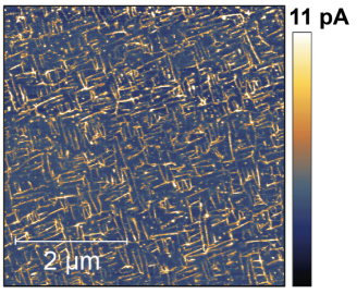
Figure 1: Conduction map (obtained using conducting force microscopy) of a ferroelectric BiFeO₃ thin layer, showing a structure of insulating ferroelectric domains (blue) and conducting domain walls (yellow). The image was obtained using conducting force microscopy at room temperature, taken from Riecketal22

Figure 1 shows a network of conducting domain walls in a ferroelectric BiFeO₃ thin layer (thickness approx. 50 nm). Electrical currents can be transmitted across the domain wall network (yellow), while the regions in between the walls are insulating ferroelectric domains that can be switched into non-volatile memory states (blue).

The properties of these materials — fine-grained conductivity pathways, local multi-stability with resistive properties that are switchable with minimal energy, many timescales, hierarchical topological structuring — hold many promises for computation in materials directly. Spatiotemporal processes in a regime ’at the edge of criticality’ near a phase transition have been described as an enabling condition for complex information processing that use such dynamics Chialvo (2010); Beggs  Timme (2012). More concretely, structures like these BiFeO₃ thin layers and other substrates, which support very large numbers of switchable and energetically interacting memory states, might become used for example to encode and dynamically switch the large random bit vectors which are the main representational elements in hyperdimensional computing Kanerva (2009) or in Hopfield networks, Boltzmann machines and other ’Ising machines’ Hopfield (1982); Ackley . (1985); Marullo  Agliari (2020); Kiraly . (2021); Zhang . (2022).

Unconventional materials and phenomena may have fascinating potentials — but whether or how these can be turned into practically relevant computing machineries and applications remains to be seen.

3 Alan Turing was a mathematician, not a physicist

One may think that we already have a shared, general formal concept of ’computing’, namely what a Turing machine can do. The Turing model of ’computing’ stands out among all other existing models. Even philosophers, when they try to come to terms with the essence of ’computing’, invariably orient their argument toward Turing computability Harnad (1994); Piccinini (2007). Its mathematical theory has been worked out far wider than any other theory of ’computing’; it is elegant and transparent; it is the most technologically productive one; and it connects ’computing’ to formal logic, which in turn yields a semantic theory of computing processes, which allows us to formally specify what a ’computation’ means with regards to solving real-world tasks. One of the consequences of the intimate connection of Turing computing with logic is that at the lowest implementation level of digital computing systems one finds the most elementary level of logical formalisms, namely Boolean logic. Digital ’computing’ models and hardware systems are built on the basis of Boolean logic gates. Almost universally across unconventional and neural modeling approaches, researchers describe ways how Boolean gates can be realized within the respective non-digital formalism. The very first comprehensive formal abstraction of brains casts it as a Boolean network McCulloch  Pitts (1943). For decades, learning the XOR function was a touchstone for artificial neural networks ML. Minsky  Papert (1969), and re-creating Boolean functions still is a standard proof of power for unconventional computing Adamatzky (2015); Bose . (2015). Efforts to implement Boolean logic in optics have been a main objective in optical computing Brenner . (1986). Emulating Turing machines in neural networks was an acclaimed achievement in the deep learning world Graves . (2016). And more often than not, formal analyses of ’computing’ done in the unconventional computing community relate back to concepts from the symbolic/digital Turing theory, for instance when discussing the potential powers of unconventional computing machines in terms of classical complexity theory Blakey (2017). Finally, and most notably, every physical system, for which physicists can offer an formal model of its states and dynamics, can be simulated on digital computers with arbitrary precision.

Given these powers and beauties of the Turing paradigm, and its undeniable role as an anchor reference for all discussions of ’computing’, why should one wish to develop a separate theory for ’computing’ based on general physical phenomena at all? What could such a theory give us that Turing theory cannot?

We begin with the historical roots of the Turing machine concept. With this formal concept, Turing set the capstone on two millenia of inquiry which started from Aristotle’s syllogistic logic and continued through an uninterrupted lineage of scholars like Leibniz, Boole, Frege, Hilbert and early 20th century logicians. The original question asked by Aristotle — what makes rhetoric argumentation irrefutable? — ultimately condensed in the Entscheidungsproblem of formal logic: is there a effective logical/mathematical method to decide (that is, find a mathematical proof) for every mathematical conjecture whether it is true or false? While all the pre-Turing work in philosophy, logic and mathematics had finalized the formal definitions of what are conjectures, formal truth, and proofs, it remained for Turing to give a formal definition of what is an ’effective’ method for finding proofs — for ’computing’ proofs — namely, that ’effectively’ carrying out a computation is equivalent to running a Turing machine.

Turing’s background concepts did not grow from intuitions about physical computing systems. He distilled his machine concept as part of a solution to a specific, deep problem of formal logic. In his famous article On computable numbers, with an application to the Entscheidungsproblem Turing (1936) — which in retrospect laid the foundation for today’s computer science — Turing conceived of his formal machine model as an abstraction of mathematical thinking. He concretely and explicitly describes how his Turing machine abstracts from a human (male) mathematician who, equipped with paper and pencil, does his mathematical thinking job. The Turing machine consists of a tape on which a stepwise moving cursor may read and write symbols, with all these actions being determined by a finite-state switching control unit. The tape models the sheet of paper used by the mathematician, the machine’s read/write cursor models his eyes and hands, and the finite-state control unit models his thinking acts. Citing from that famous article:

“Computing is normally done by writing certain symbols on paper. […] I shall also suppose that the number of symbols which may be printed is finite. If we were to allow an infinity of symbols, then there would be symbols differing to an arbitrarily small extent j. The effect of this restriction of the number of symbols is not very serious. It is always possible to use sequences of symbols in the place of single symbols. […] The behaviour of the computer at any moment is determined by the symbols which he is observing, and his ’state of mind’ at that moment. […] We will also suppose that the number of states of mind which need be taken into account is finite. The reasons for this are of the same character as those which restrict the number of symbols. If we admitted an infinity of states of mind, some of them will be ’arbitrarily close’ and will be confused.”

Turing deliberately decided for a discrete, even finitary mathematical format for his model of ’computing’. We may suspect that besides the outward reason that he gives in his article for this decision (the practical inseparability of infinitely many symbols or processing states) he also had in mind his ultimate objective of formalizing the processing of logical formulae, which are combined from a finite set of symbols and processed with a finite set of logical derivation rules. This decision to opt for finite symbol and state sets is supremely productive, as the history of DC shows. But this decision is also very restrictive. It bars the way to an immediate mathematical grasp on all ’computing’ processes that are continuous in state and time, and/or are inherently stochastic, and/or are spatially organized in physical 3D substrates — thus excluding almost all natural ’computing’ systems.

Importantly, Turing speaks of “states of mind” when he refers to the switching states of the control unit. He does not speak of physiological brain states. The Turing machine models reasoning processes in the abstract sphere of mathematical logic, not in neural physiology. Students of symbolic/digital computer science must do coursework in formal logic, not physiology; and their textbooks speak a lot about logical inference steps, but never mention seconds (we will use the acronym CS from now on to refer to the classical textbook body of symbolic/discrete computer science).

A brief philosophical aside: Different mathematicians can have different views on the ontological domains in which mathematical objects or concepts exist. A platonist mathematician will believe that mathematical objects exist in a reality that comes before the physical reality; a constructivist will believe that these objects exist to the degree that mathematicians can effectively define them together with the operations that can work on them; an intuitionist will think of mathematical objects as existing in the minds of mathematicians; and there are more such views Spalt (1981). These differences are of no concern for viewing the Turing machine as a model of a thinking mathematician. One might say that Turing himself was an intuitionist because his considerations center on “states of mind”, but we prefer to leave the classification of Turing’s philosophical stance to expert philosophers.

Turing’s commitment to the ‘thinkability’ of only discrete symbols was rooted in two millenia of Aristotelian philosophizing about logical rational reasoning. In this tradition, the existence of discrete concepts is a primary given (as opposed to the Heraclitean tradition and Christian mysticism, schools of thought that historically evolved in parallel). This Aristotelian heritage has also left its mark on linguistics and neuroscience, where it leads to the important and difficult question how analog neural systems can “think” discrete concepts and symbols. This is often mathematically modeled by attractor-like phenomena in nonlinear neural dynamics Durstewitz . (2000); Pascanu  Jaeger (2011); Fusi  Wang (2016); H. Jaeger (20211).

When one understands the Turing machine as a general model of rational human reasoning, it becomes clear why digital computers can be simulation-universal: everything that physicists can think about with formal precision can be simulated on digital computers, because these machines can simulate a physicist’s formal reasoning.

The royal guide for shaping intuitions about the physical basis of ’computing’ are biological brains, especially human brains. We will now take a closer look at what aspects of neural information processing are not captured by Turing computability.

The first thing to note is that the word ’digital’ is used outside CS sometimes in a quite generic way, pointing to anything that appears as ’binary’, ’yes-no’, ’discrete-event-like’, etc. Used in this wide sense, neural spikes and vesicle releases are frequently said to be ‘digital’.

However, within CS, the word ’digital’ has a clearly defined meaning which is much more specific than that wide-sense use. Neural spikes or vesicle releases do not qualify as ’digital’ in this specific CS sense of the word. We will explain this in some detail, because it is an important issue.

Digital computers are designed and programmed according to the principles of algorithmic computing theory. This theory is paradigmatically represented by the Turing machine model, which outside CS is the best-known model. CS textbooks however introduce numerous other formal models of algorithmic computing, e.g. lambda calculus, general grammars, logic programming, random access machines, cellular automata. They are all equivalent to Turing machines in the sense that they characterize the same set of computationally solvable input-output functions. The common denominator is that they are all based on finite sets of symbols — 0 and 1 in the special case of digital machines. All these equivalent formal models of algorithmic computing describe how symbols can be hierarchically composed into complex structures (also called ’expressions’, ’words’, ’data structures’, ’formulas’, ’programs’, ’files’ etc. depending on the context), and how these expressions can be transformed in discrete update steps according to a finite set of finitely specified rules. Specific, likewise finitely specifiable meta-rules for sequencing such rules are ’algorithms’. When a computer scientist speaks of ’digital computing’, this is metonymic usage and stands for the general principles of symbolic/algorithmic computing regardless whether the fundamental underlying symbol set is the digital symbol set $\{0,1\}$ or something else, for instance the 128-element ASCII alphabet that is used in programming languages or the digits 0–9 used in Babbage’s historical arithmetic calculator machines.

The root concept of algorithmic/symbolic/digital computing is the concept of a symbol. There exists no mathematical definition of what a ’symbol’ is - mathematicians use this concept as a primary given and can rely on a robust, shared, intuitive understanding. Tacit assumptions about ’symbols’ are that they are individually recognizable with perfect certainty; that they can be “written”; and that when they have been written they persist for arbitrary long times until they might be overwritten; and that they can be composed into words, which by definition are finite sequences of symbols. Any other data structure, like trees or tables or entire computer programs, can be 1-1 encoded into and decoded from words, thus the textbook theory of CS typically is based entirely on words. Symbolic ’computing’ processes are chains of discrete transformations of words, from an input word to an output word. It is important that a word remains immutable for indefinite timespans after it was ’written’, until it gets overwritten by some transformation operation. The immense power and mathematical as well as philosophical beauty and depth of the textbook theory of CS lies in the fact that these transformation rules can be characterized and semantically interpreted by formal logic systems, typically first-order logic, which every CS student has to learn Schoening (2008). This allows to formally specify input words as semantically interpretable encodings of ’tasks’ that are specified in a formal logic, which in turn allows CS analysts to formally prove that an algorithm does indeed precisely solve the intended task — this is the branch of CS called ’program verification’. There is a stringent connection of this logic interpretation of symbolic computing processes with the fact that digital computers (here we mean indeed the 0-1-based digital machines that surround us) operate at the lowest level with logic gates — these circuits implement the most elementary logically interpretable word update rules from which all others can be assembled.

The operations of a brain can be cast as algorithmic/symbolic/digital computing in two ways. First, one can view the brain’s operation as algorithmic. In this view, the tasks that a brain can solve are the tasks that digital computers (or any other equivalent algorithmic machine) can solve. This is the view taken in the classical work of McCullochPitts43 who model a brain as a network of logic gates. The McCulloch-Pitts neuron model allows for two activation states 1 and 0 (or active versus inactive), which are identified with the True / False values of Boolean logic variables. A McCulloch-Pitts neuron model is digital in the CS sense. Once switched to, say, a 0 value, it immutably preserves this value until its state is switched by new input. This has nothing to do with spikes — the landmark paper of McCulloch and Pitts does not mention spikes at all. If one wishes to map the abstract McCulloch-Pitts neuron to biological neurons — a very far stretch — their 0/1 values would become neuron activation values, not spike events. A McCulloch-Pitts brain is a logical reasoning machine.

The second way how a brain can be digitally modeled is to use a digital computer to numerically simulate the analog, continuous real-time, spatiotemporally organized, stochastic processes observed through physiological measurements. Then, brains are modeled by, not as, a digital system. This is in principle possible to any desired degree of approximation. Such simulation models do not give an account of the brain’s operations as symbolic-logical inferences. These simulations are just another case of using modern computers to simulate some physical system. They are good for experimentation-by-simulation, but they do not model (let alone explain) the information processing functionality of the simulated brain. Unfortunately (and importantly), the further such simulations are refined for greater accuracy, the slower they become. A spectacular, prize-winning recent example for the slowness of high-accuracy simulations of physical systems is the simulation of surface protein reconfigurations in the SARS-Cov2 virus, which kept the worldwide second-largest supercomputing cluster busy for days to simulate nanoseconds of molecular dynamics Dommer . (2021). The slowness of realistic simulations of physical dynamics quickly becomes crippling also in much more modest scenarios. In own work of co-author HJ, we tried to understand and predict the dynamics of the DYNAP-SE analog spiking neurochip Moradi . (2018) by simulation on a high-end PC, using the BRIAN software. We gave up because the simulations were orders of magnitude slower than the simulated real-time despite significant modeling simplifications, and we reverted to physical experimentation and measurements of the actual chip He . (2019).

The McCulloch-Pitts approach (and later, the view held by the proponents of the physical symbol systems paradigm) consider the information-processing functionality of brains as digital/symbolic/algorithmic systems. This approach reflects (and is limited to) a specific understanding of ’information’, which at its core is the assignment of truth values to logic expressions. In contrast, numerical simulations model the procedural mechanics of brains by digital/symbolic/algorithmic tools. Such simulations do not demonstrate or claim that the information-processing functionality of brains is the same as algorithmic computing; they do not give an account at all of what the ’information’ is that is being processed — this interpretation is external to the numerical mechanics of the simulation engine and must be supplied by the human researcher.

If one wishes to understand in what sense brains ’process information’ (or ’compute’), one needs a conceptualization of ’information processing’ for starters. One can assume (or believe or argue) that the symbolic/algorithmic/logic-based conceptualization is the right one — then the McCulloch-Pitts approach is the way to go, in its original version or in one of the later, more sophisticated variants of symbolic, logic-based AI. The challenge then is to find correlates of writable, immutable symbols in neural dynamics, and neural mechanisms that can be regarded as realizing discrete logical update rules. If one then wants to build brainlike machines, digital computers already do it natively and naturally, and there is no incentive to invest further thought in unconventional computing systems. However, we believe that the algorithmic interpretation of ’information processing’ is only partially relevant for understanding brains, namely for modeling the high-end rational reasoning functionalities, which only few animal species have developed and which even in humans is very far off from the perfect powers of formal algorithmic computing.

The mathematical tools for modeling symbolic information processing had originally been developed by linguist Noam Chomsky, who created them in order to analyse the structure of natural language and the mental operations executed by the human brain. In the high times of classical symbolic AI there was a heated philosophical debate about whether viewing brains as logical reasoning machines is an appropriate or even the only appropriate way of understanding neural information processing — or whether this is an undue simplification which prevents us from understanding biological brains and from engineering computing systems that truly deserve to be called ‘intelligent’. The former view found its most pointed expression in the ’physical symbol systems hypothesis’ stated and defended with authority by Newell  Simon (1976). Proponents of the latter position argue that the ultimate sources of biological intelligence must be sought in the apparent stochasticity and analog gradedness in human perception, reasoning, speech and action; that one cannot understand cognition as disembodied rational reasoning but that instead it realizes itself in the embodied situatedness of intelligent agents in continual physical interaction with their environments; and that self-organizing continual adaptation and learning are the key to cognition. In these views, complex symbol structures are an epiphenomenon and, for that matter, only very imperfectly realized in biological cognition. Arguments of this sort have been put forward in the philosophy of mind Clark (2013), cognitive and evolutionary linguistics Bickerton  Szathmáry (2009); Solé . (2010), cognitive science Bartlett (1932); Lakoff (1987); van Gelder  Port (1995); Hofstadter (1995), artificial neural networks Rumelhart  McClelland (1986), robotics Brooks (1995) or ‘New AI’ Pfeifer  Scheier (1999). We remark that research in neuromorphic and unconventional computing mostly unfolds in the spirit of this second perspective, although most researchers in these fields today do not engage anymore in those epistemological debates. The Turing machine certainly is a bold abstraction of a particular aspect of a human brain’s operation.

Most of the time most parts of our brain are not busy with logical reasoning. In our lives, most of the time we do things like walking from the kitchen table to the refrigerator. Yet, the kitchen-walker’s brain is thoroughly busy with the continual processing a massive stream of sensor signals, smoothly transforming that input deluge into finely tuned, uninterrupted command signals to hundreds of muscles. We like to call this processing of sensorimotor flows of information the ’cybernetic’ mode of computing. For the largest part of biological history, evolution has been optimizing brains for cybernetic processing — for “prerational intelligence” Cruse . (2013). Only very late, some animals’ brains acquired the additional ability to detach themselves from the immersive sensorimotor flow and generate logico-symbolic reasoning chains. Several schools of thinking in philosophy, cognitive science, AI and linguistics explain how this ability could develop seamlessly from the cybernetic mode of neural processing, possibly together with the emergence of language Bradie (1986); Greenfield (1991); Drescher (1991); Pfeifer  Scheier (1999); Lakoff  Nunez (2000); Fedor . (2009).

4 The structure of theory systems of physical computing systems

In the Introduction we argued that a practically useful formal framework for computing systems will likely not come in the form of a single core theory (like the theory of Turing machines), but that instead it will have to consist of a network of interrelated subtheories that span the modeling levels from physical hardware to task specification formalisms (like the theory canon of CS textbooks, which contains the Turing machine model as one among other subtheories). In this section we propose a general schema for such a hierarchy of subtheories. This schema is not itself a theory of physical computing systems but an organization plan to design them. Its usefulness lies in making us aware of the multiple facets of the theory-building problem, and in clarifying how different subtheories should interconnect.

To distil such a general schema of subtheory organization, we started from previous studies by Horsmanetal14 who proposed an abstract model of computing systems, intended to capture all currently discussed sorts of ’computing’ systems; and from Jaeger21a who analysed and unified three quite different kinds of modeling frameworks for information-processing systems — the classical CS theory body; probabilistic models based on stochastic sampling; and approaches based on self-organizing adaptive dynamical systems. Together these two studies converge to a picture of general ’computing’ system models that is drawn around three fundamental requirements:

1. modeling ’computing’ systems must include modeling their physical basis;

2. there must be formalizations of information processing mechanisms which transform input information to output information (and there must be models of input and output ’data’ in the first place);

3. modeling ’computing’ systems must include a semantic subtheory that allows us to formally specify the real-world tasks served by the computing system and that gives an account of the meaning of computational operations.

Together with the four goals that we mentioned in the Introduction (phenomenal openness, interpretability, scalability, abstraction), these three theory-architecture requirements present a set of constraints that is not easy to accomodate.

The studies by Horsmanetal14 and Jaeger21a present box-and-arrow diagrams for the structure of theory systems for computing systems. We merged structural ideas from both sources and added new elements and detail in order to make it more concrete and instructive. An overview of our extended schema is given in Figure 2.

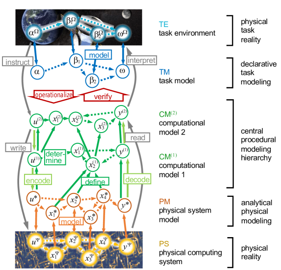
Figure 2: An organization schema for a complete modeling hierarchy of computing systems. The central element is a hierarchy of computational models CM^(m), which formalize transformation processes from input encodings $u^{(m)}$ through intermediate information-carrying states $x_{i}^{(m)}$ to output encodings $y^{(m)}$ (two levels shown). This central procedural modeling hierarchy is sandwiched between two sides of physical reality: the physical computing system PS and the real-world task environment TE, to which it interfaces through an analytical physical system model PM and declarative task model TM. (Top background image from MITNews19)

The circled items and arrows in this figure mean different things in the various layers. In the physical computing system PS we posit physical input states $u^{\Psi}$, intermediate machine states $x_{i}^{\Psi}$ and output states $y^{\Psi}$. Our use of the word ‘state’ needs an explanation. Physicists speak of the state of a system when they mean the totality of the system’s physical condition at a given moment in time Zadeh (1969). We call this a global (or total, or system) state. In contrast, the circled nodes in the PS layer in our diagram represent partial states — aspects or components of the global state that can be spatially localized or otherwise isolated and physically measured, at least in principle. At different moments in time these local states can yield different measurement values. For instance, some $x_{i}^{\Psi}$ could be a contact point in an electronic circuit where voltages can be measured; or it could physically extend to an entire microchip of which the overall temperature is measured. The yellow broken arrows in PS represent physically causal influences. All circles in layers PS, PM, CM^(m) are meant to denote partial states. For simplicity we will just say ‘state’ when we mean partial states. When we do not want to distinguish between input/intermediate/output states $u,x,y$, we use the generic symbol $v$.

The physical system model PM hosts 1-1 formal representatives $v^{\ast}$ of physical states $v^{\Psi}$. These $v^{\ast}$ are abstract, formal items — state variables. The broken brown arrows in PM stand for formal models of causal interactions. Often this will be the couplings between state variables in systems of ordinary differential equations (ODEs). All variables $v^{\ast}$ in PM are time-dependant with regard to the standard model of time $t[\mbox{sec}]\in\mathbb{R}$ that is used in the natural sciences; thus we could also write $v^{\ast}(t)$. The relation between PS and PM is the scientific modeling relation of the natural sciences and engineering: physical states $v^{\Psi}$ must in principle be measurable, and the causal interaction models in PM must lend themselves to generate falsifiable predictions about the states $v^{\Psi}$. The model PM is created by hardware engineers or natural science experts (for instance biologists if PS is a biological substrate). PM is an analytical model (as opposed to a blackbox model), in that it aims at capturing the causal mechanisms that according to expert insight are active in the material computing system.

The state variables $v^{(1)}$ in the first computational model CM⁽¹⁾ are formally defined in terms of $v^{\ast}$ variables (solid dark green arrows). There may be more or fewer state variables in CM⁽¹⁾ than in PM. CM⁽¹⁾ is equipped with stochastic or deterministic, possibly recursive transformation rules which ultimately determine the values of the output variable $y^{(1)}$ from values of the input variables $u^{(1)}$ via intermediate variables $x_{i}^{(1)}$ (broken green arrows). The values of these variables can be mathematical objects of many sorts: numbers, vectors, symbols, distributions or other set-theoretic constructs. Determination pathways may contain cycles. When we say ’determine’ we do not necessarily mean a deterministic transformation relation, but intend any sort of an effective fixation of output values. Thus, the broken arrow from $u^{(1)}$ to $x_{1}^{(1)}$ in Figure 2 may refer to a deterministic function, or a probabilistic law, or a non-deterministic choice between possible values of $x_{1}^{(1)}$. As a special condition, $u^{(1)}$ must be defined exclusively from $u^{\ast}$ and $y^{(1)}$ from $y^{\ast}$.

In the digital world, CM⁽¹⁾ would be the direct machine interfacing layer where the machine instructions are resolved to bit switching operations determine the values of binary state variables $v^{(1)}$ (this model is used by the microchip engineers but usually not communicated to customers or programmers).

Higher-up computational models CM^(m), if present, are defined from the respective next lower model CM^(m-1) in a similar way. Figure 2 shows a case with only two CM layers. In the digital world this would correspond, for instance, to software abstraction layers connected to each other by simulation/compilation. In the digital world the model CM⁽²⁾, which lies directly above the bit-level machine interface model CM⁽¹⁾, could be the machine instruction level provided by a microchip manufacturer, or a model written in assembler code. The highest-level model CM^(K) would be expressed in a high-level programming language or graphical user interface language. In the digital domain these higher models CM${}^{(2)},\ldots,$ CM^(K) would be created by programming experts in the case of programming a concrete computer, or by theoretical computer scientists in the case of general formal analyses.

It must be formally specified how input formats $u^{(m)}$ defined in CM^(m) become encoded in inputs $u^{(m-1)}$ in the respective next lower computational model CM^(m-1). Conversely, output formats in the various modeling layers are related to each other by upward decoding rules. The decoding rules can be formulated in a different formalization language than the formal definitions of $y^{(m)}$ from $y^{(m-1)}$.

A computational model CM^(m) specifies a dynamical system, whose temporal evolutions — which we will call ’runs’ or ’executions’ in accordance with computer science terminology — are the computations carried out by CM^(m). The broken green arrows in Figure 2 stand for the dynamical laws that govern the computations. An arrow from $v_{i}^{(m)}$ to $v_{j}^{(m)}$ means that the law by which $v_{j}^{(m)}$ changes its value in time is co-determined by the values of $v_{i}^{(m)}$. Each variable $v_{i}^{(m)}$ has its own local value change law — we will call it its update rule. Update rules can be deterministic, probabilistic, or non-deterministic. All these update rules together give the complete dynamical law for CM^(m). When we say that a model CM^(m) is executed, we do not necessarily mean that it is run on a real physical machine. Demanding that a computational model CM^(m) is executable only means that it specifies data transformations which can be mathematically traced from input to output. All relations between inputs and outputs which one deems relevant must be mathematically provable on the basis of CM^(m). Most Turing machines that are described in textbooks are never physically executed.

All broken and solid arrows in and between PM, CM⁽¹⁾, $\ldots,$ CM^(K) together should make for a commuting diagram in the mathematical sense. This entails that if the highest-level output $y^{(K)}$ is obtained from the input $u^{(K)}$ along two pathways in our schema — the first one horizontally using the transformations within CM^(K), the second one first going down vertically through an encoding sequence until $u^{\ast}$, then horizontally within PM to $y^{\ast}$ and finally decoding upwards again until $y^{(K)}$ is reached — the two versions of $y^{(K)}$ thus determined should come out with (approximately) the same value. The required degree of approximation is a matter of convention in a given designer/user community. In the DC world the agreement has to be exact. Also all other horizontal versus down-horizontal-up path pairs between variables in various CM^(m) should commute (Figure 3). In the AC theory literature, commuting diagrams are an important algebraic tool for formulating consistency conditions between model refinement levels. To our knowledge, in the physical computing literature this commuting diagram condition has been first clearly stated by Horsmanetal14, where a new aspect was that it refers to equivalence between formal and physical state transformation pathways.

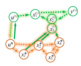
Figure 3: Paths in a modeling hierarchy should commute. The graphic shows an excerpt from Figure 2 with two path bands (orange and green shadows) from source $u^{(1)}$ to target $x_{2}^{(1)}$. Such paths must include all loops (here e.g. $x_{2}^{\ast}\to x_{4}^{\ast}\to x_{3}^{\ast}\to x_{2}^{\ast}$) and parallels (here: $u^{\ast}\to x_{1}^{\ast}\to x_{2}^{\ast}$ and $u^{\ast}\to x_{2}^{\ast}$) which are touched on the way from the source to the target. The two versions of the target determined by the two transformation paths (here: the two $x_{2}^{\ast}$ nodes with the orange resp. green shadows) must have approximately the same value. Similar commutativity constraints must hold between all levels in the hierarchy PM, CM${}^{(1)},\ldots$, CM^(K).

The top layer in Figure 2 depicts the real-world task environment TE where the user of the computing system specifies a computational task, often in plain natural language, in terms of initial givens $\alpha^{\Omega}$ and desired outcomes $\omega^{\Omega}$, possibly with subgoals $\beta_{i}^{\Omega}$. These items may be connected by more or less precisely described means-ends conditions (broken turquoise arrows). The complexity of our real world will often hinder the identification of well-defined partial states or observation procedures.

The informal and possibly opaque task description given by an end-user is captured in a formal task model TM which again models the initial givens, subgoals, desired outcomes and the means-ends conditions perceived by the user. The modeling relation between the real task environment and its formal model is much less well-circumscribed than the modeling relation between PS and PM. There is no generally followed method that would be equivalent to the predict-test-refine modeling cycles of the natural science paradigm. In the digital world, task models TM are mostly specified in a logic formalism. In classical AI applications they are created by trained knowledge engineers Feigenbaum (1977).

The formal representation $\alpha,\beta_{i},\omega$ of initial givens, subgoals, and final outcomes is less clear than in the case of the PS-PM relation. In AI formalisms these representatives may become extensive logical formulas which only partly describe observable and identifiable real-world conditions, in contrast to the largely unequivocal representations of physical measurables in PM. In statistical formalizations, $\alpha,\beta_{i},\omega$ may denote probability distributions, and in dynamical systems approaches they may reflect qualitative phenomena like attractors or bifurcations H. Jaeger (20211). Similarly, the specific formal nature of interrelations and interactions between $\alpha,\beta_{i},\omega$ (broken blue arrows) depends on the formal modeling framework that is used, to be interpreted as causal, correlational, or logical relations. Task models may or may not be dynamical systems models. They may or may not be executable, and the typical case is that they are not. The operationalization, which designs the highest-level computational model CM^(K) from TM, in any case leads to an executable dynamical system model.

There is a wide conceptual and formalism gap between the task model TM and the highest computational model CM^(K). How this gap can be bridged is one of the most challenging acts in modeling a complete computing system. In the digital computing domain, this is the objective of program verification, for which a compendium of subtle and demanding methods has been developed. With regards to a general theory of modeling computing systems we cannot say much at present. A core difficulty of connecting TM with CM^(K) is that TM will often only specify the givens and goals without indicating the effective mechanisms needed to solve the task, while conversely the formalisms used for computational models CM^(m) can codify mechanical data transformation mechanisms but have no native means to encode what the data structures mean in terms of task conditions. In the terminology of computer science this is the distinction between declarative (in TM) versus procedural (in CM^(m)) specifications.

A naive end-user of a computing system will normally be unaware of the formalizations TM, PM, CM⁽¹⁾, $\ldots$, CM^(K-1) and only use the highest-level computational model CM^(K) in the format of a high-level programming language or graphical user interface. The grey arrows in the graphic depict the main interactions of an end-user with a computing system. He/she knows how to directly instruct the computing system about the task initial conditions $\alpha^{\Omega}$ in terms of input formats $u^{(K)}$ and how to physically write $u^{(K)}$ values to the physical input states $u^{\Psi}$, for instance by hitting a keyboard. Similarly the user must know how to read physical outputs (for instance illuminated pixels on a screen) as formal computation results $y^{(K)}$, and interpret $y^{(K)}$ as real-world task outcomes.

All of these grey-arrow operations cross the ontological border between abstract formalism and physical reality. Likewise, the two modeling relations between TE and TM, and between PM and PS, cross this border. These ontological transitions are not a proper part of a formal theory computing systems. They represent conditions of its practical use, human judgement and engineering craftmanship. We consider only the formal layers PM, CM^(m) and TM as a model of a computing system. In Jaeger21a we called the layers PM and CM^(m) “how-models”: they capture the procedural mechanics in a computing systems. In contrast, the task model TM is a “what-model” in that it specifies the semantics (goals and real-world setting) of a computation.

Our schema of models of a computing system may look overly complex compared to the simplicity of the Turing machine model. Our schema has, however, a wider scope than the Turing machine model: we aim at providing a general conceptual coordinate system for discussing all the modeling levels that are needed to establish a full-scope engineering discipline of general computing systems, from physical substrates to ‘programming’ layers to use-cases. The digital theory canon offers dedicated, rigorously interconnected formal subtheories for all layers in our schema. It minimally comprises the theories of Boolean logic, formal languages, computability, computational complexity, and first-order logic. The Turing machine model can be positioned at any of the CM^(m) levels, depending on how closely the physical system model PM resembles a Turing machine. If the hardware is built with a re-writeable tape for a memory mechanism (as in some museum exhibits), the Turing machine model would sit at the lowest-level CM⁽¹⁾. If a Turing machine is simulated on a PC via a tutorial graphical interface, the Turing machine model would come out as the highest-level model CM^(K).

We conclude this section with a comment about our commitment to state-based transformation formalizations in the computational models CM^(m). CS textbooks include various formalisms that specify the class $\mathcal{C}$ of ’computable’ functions $f:\mathbb{Z}\to\mathbb{Z}$ by non-deterministic operations. Examples are the classical, pre-Turing specification of the recursive functions, lambda calculus, type-0 grammars and other non-deterministic term rewriting formalisms, including sets of inference rules for first-order logic. However, when any of these formalisms is to be used for ’effective’ computing, the inherent non-determinism in these specifications of $\mathcal{C}$ becomes changed into deterministic processing mechanisms by adding constraints, for example by requiring a specific evaluation order for lambda calculus (which leads to functional programming languages) or heuristic search restriction rules (for term rewriting systems and logic formalisms, leading to automata realizations of grammars or implementations of the PROLOG logic programming language). These derived procedural models are then state-based, and only they can be ’executed’ by machines. As far as we can see, in the field of CS only deterministic machines are used in practice. In principle it is also an option to add constraints which change such non-determistic models of $\mathcal{C}$ to probabilistic models, which would lead to physically executable, state-based, stochastic input-output transformations. This avenue seems not to be exploited in mainstream CS. Again, such probabilistic models would be state-based. Since our main objective concerns physically executable models of ’computing’, we opt for a state-based, procedural view on computational models CM^(m), in a physics/engineering mindset.

5 Algorithmic and cybernetic theory hierarchies

As we will soon explain, in our fluent computing approach toward a GFT we combine ideas that originated in algorithmic computing (AC) with ideas from the cybernetic computing (CC) world. In this section we describe relevant aspects of both views in more detail, contrasting a schematic algorithmic model hierarchy with a cybernetic one. Figure 4 casts a glance at the venerable historical context of our endeavours.

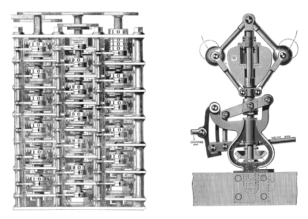
Figure 4: Left: The paradigmatic algorithmic computing machine: Charles Babbage’s difference engine No. 1 (Harper’s new monthly magazine, December 1864). Right: The paradigmatic cybernetic information processing machine: the centrifugal governor (Drawing from W. Ripper: Heat Engines. Longman, London 1909). Both figures found in Wikemedia Commons.

The central segment in our generic schema for structuring GFTs (Figure 2) is the hierarchy of computational models CM^(m). In Figure 5 we place two such CM^(m)-hierarchies side by side, the first one highlighting how such hierarchies are modeled in an algorithmic spirit (panels a–c), while the second one illustrates how we see cybernetic computing (e–g; d and h will be discussed later). We picture three modeling levels each. At the top (CM⁽³⁾) we show a model of a computational process as it might exist in the mind of an entirely naive end-user, who knows nothing about the inner workings of the computing machine and only has a global understanding of the task’s input-output transformation. In the middle (CM⁽²⁾) we draw a schematic of how this global model is more concretely instantiated as a computer program by a CS programmer (left) or as a system configuration by a cybernetic system engineer (right). At the bottom we picture a close-up in CM⁽¹⁾ of a part of the CM⁽²⁾ model, in which a sub-mechanism of CM⁽²⁾ is detailed (compiled, down-engineered) to a level of detail that is suitable for getting directly mapped to the underlying hardware. To make our discussion concrete, we exemplify our explanations with the elementary algorithmic task of multiplying 6 with 5 on a pocket calculator Schroeder (2022), and the paradigmatic cybernetic task of regulating the speed of a steam engine with a centrifugal governor Maxwell (1886).

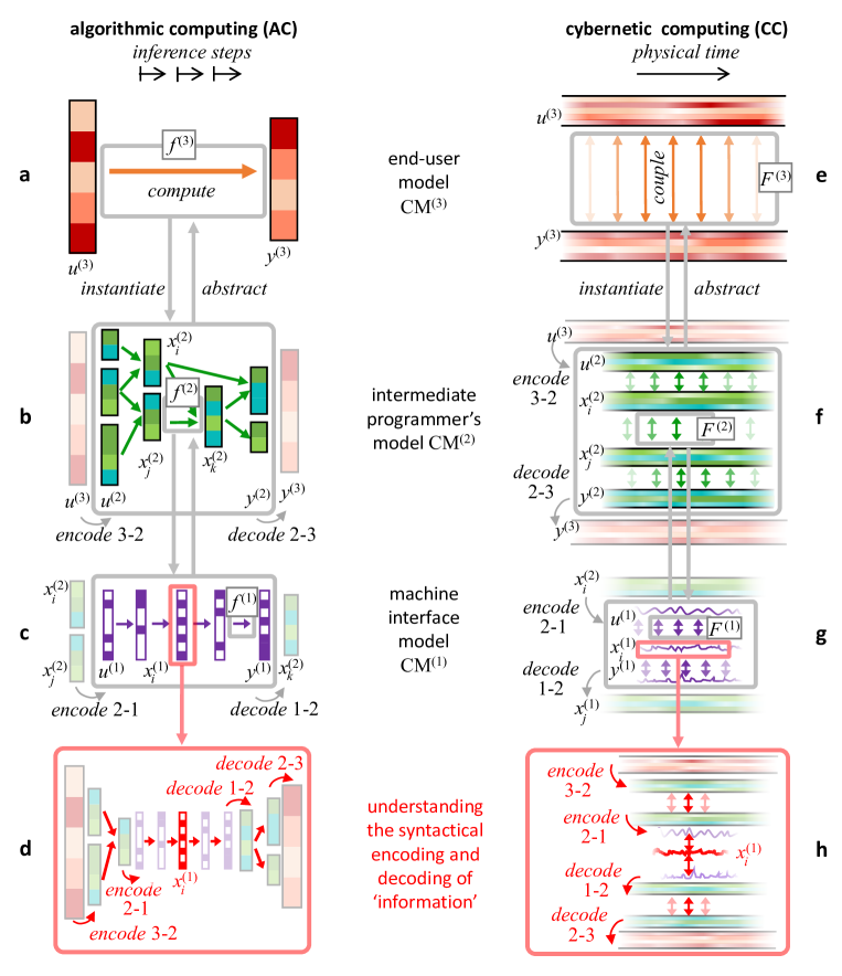
Figure 5: Schematic of algorithmic (left, a–c) and a cybernetic (right, e–g) modeling a computation on three levels. Bottom panels d, h in red highlight the different interpretations of ’information processing’. For explanation see text.

We begin with the algorithmic dissection of the 6 $\times$ 5 multiplication task (left part of the figure). Digital computations are theoretically modeled and practically programmed by breaking down the overall input-output function $f^{(3)}$ to a low-level machine interface formalism, through a cascade of increasingly finer-granular formalisms — think of compiling a program written in a high-level programming language like Excel down to machine-specific assembler code, passing through a series of programs in languages of intermediate abstraction like Python or C. On the top level CM⁽³⁾ in our pocket calculator example, the user specifies task instances by typing the input string $u^{(3)}=$ 6 * 5, then pushes an ’enter’ button and expects the result $y^{(3)}=$ 30 to appear in the display. In our graphic in panel a the structure of the input 6 * 5 is symbolized by the cells in the vertical state bars, and the specific values 6, *, 5 by colors. The user knows that there is a mathematical function $f^{(3)}$ (the multiplication of integers) which is evaluated by the calculator, but what happens inside the calculator of no concern to a naive end-user. The technical details are taken care of by the designers of the calculator, who hierarchically break down the processing of inputs like 6 * 5 down to a model CM⁽¹⁾, which matches the available physical elements in the hardware and thus can be mapped to the logic gates and memory cells of the digital hardware.

On an intermediate modeling level CM⁽²⁾ the system designer might encode the original input $u^{(3)}=$ 6 * 5 in a binary representation (for instance 6 $\mapsto$ 1 1 0, 5 $\mapsto$ 1 0 1, * $\mapsto$ binarymult (leftmost green cell bars $u^{(2)}$ in panel b). This new input encoding is then processed stepwise with functions $f^{(2)}$ (green arrows), possibly in parallel threads, through sequences of intermediate binary representations $x_{i}^{(2)}$, until some binary string representation $y^{(2)}$ of the result is obtained, which then can be decoded into the top-level representation $y^{(3)}=$ 30. One of these functions $f^{(2)}$ (inner gray rectangle in panel b) could for instance be a binary addition operation $x_{i}^{(2)}+x_{j}^{(2)}=x_{k}^{(2)}$, corresponding to binaryadd(1 1 0, 1 0 0) = 1 0 1 0.

In a final compilation, this instance of the binaryadd operation might become encoded in a sequence of 8-bit string transformations, whose outcome $y^{(1)}$ decodes to $x_{k}^{(2)}=$ 1 0 1 0. This encoding format can be directly mapped to a suitably structured digital hardware by an experienced engineer. In our schematic diagram we assume that this level specifies Boolean functions $f^{(1)}$ (violet arrows in c) between 8-bit rewriteable register models (vertical violet bars). The intermediate level-2 bit structures $x_{i}^{(2)}$, $x_{j}^{(2)}$ become encoded to the 8-bit register pattern $u^{(1)}$, which serves as the initial state for the level-1 processing of $f^{(2)}$.

We now turn to our view on hierarchical models of cybernetic information processing systems (e – g). On all levels $m$, inputs $u^{(m)}$ and outputs $y^{(m)}$ are signal streams that are continually received / emitted. These signals can be composed from subsignals — think of a robot’s overall sensory input which might comprise subsignals from cameras, touch sensors, the battery status and joint angles. This multi-subsignal makeup is reflected in Figure 5 by the stripes inside the $u^{(2)}$, $y^{(2)}$, $u^{(1)}$, $x_{i}^{(1)}$ and $y^{(1)}$ bands, and the time-varying subsignal strengths by changing color intensity. The decomposition into subsignals may be hierarchically continued. In the figure only the first-level subsignal structure is shown.

At the lowest machine interface level $L^{(1)}$ (panel g), input/output signals $u^{(1)}$ and $y^{(1)}$ as well as intermediate processing signals $x_{i}^{(1)}$ are modeled as evolving in real time $t\in\mathbb{R}$. At higher modeling levels, more abstract mathematical models $\mathfrak{t}$ of temporal progression may be used, allowing for increasing uncertainty about precise temporal localization (explained in more detail in Section 2.4 in JaegerCatthoor23). We will reserve the word ’signal’ for one-dimensional, real-time signals, and use the word ’chronicles’ to refer to possibly multi-modal signals that are formalized with possibly more abstract time models $\mathfrak{t}$.

In our steam engine governor example, the highest-level input chronicle $u^{(3)}$ would be composed of the measured current engine speed $s^{(3)}(t)$ and the desired speed $d^{(3)}(t)$. The output chronicle $y^{(3)}$ is the controlled steam valve setting signal $p^{(3)}(t)$. The input and output chronicles are continually connected by a coupling law $F^{(3)}$, in our governor example for instance by the simple proportional control rule $\dot{p}^{(3)}=K\,(d^{(3)}-s^{(3)})$. While in this example, the coupling is unidirectional from $u^{(3)}$ to $y^{(3)}$, in general we admit bidirectional couplings. In the terminology of signals and systems, we admit autoregressive filters for coupling laws. We note that the reafference principle in neuroscience Jékely . (2021) stipulates that output feedback is common in biological neural systems.

While in the governor example, the highest-level input chronicle $u^{(3)}$ is composed of two signals which are not further subdivided, in general a chronicle can be composed of sub-chronicles which in turn can be compositions of sub-subchronicles, etc. Chronicles are hierarchically structured signal objects (deeper nesting detail not visualized in our figure).

An intermediate CM⁽²⁾-model would capture the principal structure and dynamics of the governor, using chronicles that monitor speeds, forces, angles etc. of system components like masses, levers, axes, joints etc.

On the lowest level CM⁽¹⁾, the dynamical couplings between CM⁽²⁾-chronicles are concretized to match the specific design of a concrete physical governor. For instance, a coupling $F^{(2)}$ between a centrifugal force and a compensating gravitational load force (inner gray box in panel f), which would presumable be formalized in CM⁽²⁾ by a differential equation, would be further resolved in CM⁽¹⁾ to the metric positioning of joints on lever arms, the weights and sizing and strengths of mechanical parts, etc., leading to fine-grained signals $u^{(1)}$, $x^{(1)}$, $y^{(1)}$ like the current force or velocity components on a specific joint, or — in a high-precision model — measures of temperature or vibration which have an impact on the part’s functioning.

The algorithmic–cybernetic distinction is not a clear-cut either-or division. An intermediate view on ’computing’ is adopted in models of analog computing Shannon (1941); Blum . (1989); Moore (1996); Bournez  Pouly (2021). Such modeling strategies follow the algorithmic paradigm in that a high-level function evaluation task is hierarchically broken down into lower-level flowchart diagrams of sequential function evaluations like in our diagrams a–c. At the same time they also appear as cybernetic in that their data structures are composed of analog real numbers, and the functions $f^{(m)}$ are evaluated through the continuous-time evolution of differential operators. In another tradition (branching off from CS), the input-output theory of algorithmic computing has been variously extended to sequential processing models, for instance through the concept of interactive computing Wegner  Goldin (2003) and (symbolic) stream computing Endrullis . (2019).

Both digital computers and brains are commonly said to ’process information’. One might hesitate to call the centrifugal governor ’information-processing’ too, but we see it as a member of the large family of dynamical input-output transforming cybernetic systems that also contains brains, and will thus consider even such simple regulators as information-processing. ’Information’ is an iridescent concept. When one is serious about characterizing computing machines as ’information-processing’, one should have a clear understanding of this concept. Algorithmic and cybernetic models of computing systems lead to different conceptualizations of ’information’.

Information is information about something, encoded in something else. Full accounts of ’information’ thus should cover semantics (aboutness) as well as what one may call syntax (formats of information-encoding formal objects). The semantics of what is computed by some machine relates to the external task, or more precisely, to the understanding that the user of the machine has of the task. The syntax becomes manifest in the data structure and processes that are used in some computational model. The eternal intellectual challenge to come to terms with meaning has spawned a diversity of formalizations created under different scientific perspectives. Examples are the semi-formal theories of semiotics in linguistics Eco (1979) and the theory of pragmatic information where information is captured through its impact on the belief states of a receiver of information beim Graben (2006), to name only two approaches that are couched in centuries of philosophical debate. We have discussed semantical and syntactical aspects of ’information’ in computing systems in more detail elsewhere H. Jaeger (20211), where we called these two sides the ’what’ and the ’how’ aspects of information processing. Because it is an important topic, we here give a summary, referring to the panels d and h in Figure 5.

The algorithmic CS theory offers a full account of semantics and syntax. The syntactical ’how’ aspects are covered in CS theory textbooks about automata and formal languages, and in practically oriented textbooks about computer architectures and programming languages. It is mathematically clear how system models at different abstraction levels CM^(m) can be equivalently en- and decoded into each other. Students practice this in homework exercises, and compiler or interpreter programs do it mechanically. If one wants to elucidate what role is played by the creation and subsequent transformation of a machine-interface data object $x_{i}^{(1)}$ (Figure 5d), the contribution of this nanosecond event to the successful computation of the user’s task input can be precisely determined (and debugged if needed) by unraveling the cascade of hierarchical encodings, inference steps, and decodings that lead from the task input $u^{(3)}$ down to $x_{i}^{(1)}$ and back up to the task output. Furthermore, the semantical ’what’ aspects are covered by formal logic, whose semantic theory (called model theory) can precisely relate all syntactical structures and operations to set-theoretic structures, which in turn are formal models of a user’s conception of the task. This is taught to students of computer science in mathematical textbooks of formal logic and practical textbooks of program verification.

We do not possess a textbook theory of cybernetic computing that comes anywhere close to the completeness of the CS theory cosmos. There is an obvious plausible candidate for a formal account of ’information’ in cybernetic computing, namely Shannon information theory. Tools from this theory are widely used in signal processing and control, theoretical neuroscience, statistical physics and complex systems science — all of these being concerned with dynamical, open systems that are akin to our view on cybernetic modeling from Figure 5. Shannon information theory can quantify the information in signals (or chronicles) and calculate the information gain or loss when stochastic signals are transformed (filter operators $F^{(m)}$ in Figure 5) or encoded and decoded from one format to another. Referring to Figure 5h, the information contribution of a lowest-level signal $x_{i}^{(1)}$ to the highest-level task chronicles could be quantified and tracked through the en/decoding hierarchy and the coupling processes that concern $x_{i}^{(1)}$. Shannon information is framed in probability theory. Methods from probability theory are widely used in signal processing, when signals are formalized as stochastic processes. Some models of information processing in machine learning or computational neuroscience are expressed in terms of operations on probability distribtions, for instance dynamic Bayesian networks Murphy (2002), statistical physics models like the Boltzmann machine Ackley . (1985), or neural sampling models Pecevski  Maass (2011). The computational processes in such models are often based on sampling, which is a genuinely probabilistic way of ’running’ such models. Jaeger21a discusses sampling-based models of computing in some detail. Shannon’s theory can naturally serve as an interpretation of ’information’ in such models.

Furthermore, the rooting of Shannon information theory in probability theory could yield a semantic interpretation of a user’s task model, which would be formalized as the probability space that generates the input and output signals. Like the logic-based semantical models of CS, probability spaces are richly structured sets, formalized directly in the langauge of set-theory. Textbooks of information theory Cover  Thomas (2006) unfortunately do not mention or pursue these probability-theoretical underpinnings, which could lead a way to a semantic theory for Shannon information.

Although Shannon information theory appears a natural candidate to understanding ’information’ in cybernetic models, we are skeptical whether it is the ultimate answer. Casting a cybernetic theory firmly in a framework of probability might be procrustinating, and for understanding qualitative phenomena in nonlinear dynamical systems (attractors, bifurcations and more), which may be important for computing functionality, we have come to the conclusion that novel formal tools for capturing their ’how’ and ’what’ are needed H. Jaeger (20212).

Summarizing our contrasting of AC versus CC modeling, we find that online, real-time, brain-like, cybernetic transformations from input signal streams to output signal streams is in some aspects similar to, and in other ways fundamentally different from algorithmic computing. The similarities justify to classify cybernetic computing as ’computing’ in the first place. We wrap up the differences in a punchline: Algorithmic models of computing systems capture the processing of structures, while cybernetic models describe the structure of processes.

6 Big challenges ahead

Our schema from Figure 2 is just that, a structure schema for theory systems for physical computing systems. It is not itself a theory. Yet, this schema already allows us to identify and discuss problems that at present still limit our abilities to engineer general non-digital computing systems. In the domain of digital computing, these problems often are non-issues, but they become fundamental in physical computing.

Which physics?

Any given slab of physical material hosts an large number of principally observable local states $v^{\Psi}$ (Figure 2) — infinitely many for all practical purposes. They differ in spatial extension (from individual magnetic spins and voltages at electronic contact points to extended electrical or magnetic fields or the global temperature of the entire slab), time constants (from molecular configuration flips to ultra-slow reconfiguration of crystal structures), or complexity (from a simple capacitor charge to highly organized resonance patterns like skyrmions). New kinds of identifiable and measurable nanoscale phenomena continue to become discovered as materials science progresses. Their number explodes when one considers the possible kinds of dynamical interactions between them and their susceptibility to external physical inputs. This raises the question which local states $v^{\Psi}$ and their modeling variables $v^{\ast}$ are chosen as a basis for the physical model PM, and how to fabricate material systems PS that reliably realize this choice. Or, asking the reverse question, if one wishes to realize in hardware some computational model CM^(m), which materials and phenomena can support the state constructs $y^{(m)}$ from that model? While today the standard choice for silicon physical substrates is to focus on electronic observables, silicon wafers can also be processed into computing systems whose mode of operation is mechanical Coulombe . (2017); Dubcek . (2021) or optical Freiberger . (2017). A consequence of this phenomenal openness is a lack of guidance for materials scientists as to which sort of physical effects, exactly, they should target and optimize in their novel computational substrates.

In the light of this richness of options it is no surprise that it is not clear at present which states in biological brains are the relevant ones to explain neural information processing: the states of individual synapses, dendritic branches, neural potentials, activity patterns in neural microcircuits, or extended neural fields — or which combination of these at which levels of resolution? In terms of our generic schema in Figure 2: which physical model PM of a brain would be needed to obtain all cognitively relevant computations by defining hierarchies of computational models CM^(m) on top of PM?

What’s the time?

Computing systems transform input to output. On the physical level PS, this happens in physical time, which can be measured with physical clocks. Physical system models PM typically (maybe necessarily) use the real-valued timeline $t[\mbox{sec}]\in\mathbb{R}$ as formal model of time, either directly as in ODE models, or in a sequence of sampling intervals $(n\,\Delta t[\mbox{sec}])_{n\in\mathbb{N}}$ as in formal models of digital signal processing or time-discretized physical models of digital microchips. Above the PM modeling level many other formal models of time may be chosen, which are increasingly abstracted from physical time $t[\mbox{sec}]$. An extreme case of temporal abstraction occurs in the Turing machine. The update steps that lead from one Turing machine configuration state to the next one are, in a deep sense, timeless. All that is left is the strict sequential ordering of configurations. This ordering is of a logical rather than a temporal nature: Turing devised of his “machine” as a model of logical reasoning steps. He made it a point that these are decoupled from physical time: “It is always possible for the computer to break off from his work, to go away and forget all about it, and later to come back and go on with it” Turing (1936) — provided that “the computer” left a written note to remind him later at which stadium in the computation he took a break. The formal model of time in a Turing machine reduces to a sequence $s_{0}\Rightarrow s_{1}\Rightarrow\ldots$ of update steps that is ordered purely by logical implication. Thus, in a formal model of a computing system, which has the Turing machine in one of its levels CM^(m), the question arises how Turing state variables $v^{(m)}_{i}$ and their logical progression links (broken green arrows in Figure 5) can be formally defined on the basis of a physical system model PM that uses physical time $t[\mbox{sec}]$. If one starts to seriously think about the problem of formalizing time and deriving formal hierarchies of increasingly abstract models of computational progression, one faces a host of conceptual and mathematical questions relating to time constants, timescales, synchronization, online vs. offline processing, models of temporal reactivity and memory span hierarchies that awaits a systematic treatment. JaegerCatthoor23 draw an initial systematic chart of models of temporality (called “modes of progression” there) in computational models, and survey about twenty partial models and formal transformations between models of temporality that have been proposed in digital computer science, computational neuroscience, dynamical systems theory and machine learning. In the present article we will use the symbol $\mathfrak{t}$ when we want to refer to any mathematical model of temporal progression.

We mention in passing that the problem of modeling temporality comes with a twin problem of abstraction hierarchies of spatial scales that spans from metric physical space to abstract topological spaces.

How fast does time go by?

Digital computers employ two basic physical memory mechanisms by which bit values are preserved over time: the fixed-point attractor stabilization of a high or low voltage in the logic gate circuit electronics — this has a memory span of one clock cycle; and the unbounded-duration storage of bit values in non-volatile memory devices. By writing to and reading from memory devices, digital computer programs can perfectly preserve bit values over any memory span between a clock cycle and infinity. This is of obvious importance for executing symbolic program code: a value that has been assigned to a variable must be reliably retrievable through that variable at any later time where it will be needed.

This is in contrast to biological brains where a plethora of physiological mechanisms and anatomical structures are dedicated to the encoding, transporting through time, and decoding memory items. These mechanisms operate physically in a wide spectrum of timescales in a fine-tuned concert. The brain’s owner can recall previous experiences through a seamless range from milliseconds to lifetime without being aware of multitude of neural mechanisms that are invoked. In unconventional computing hardware — analog neuromorphic microchips in particular — perfectly non-volatile memory devices are often not available. Hardware engineering under fabricability constraints typically can supply only a small choice of physical effects for memory devices and memory subsystems, each of which is volatile and supports memory spans in a limited timescale interval only. Very long timescales are especially difficult to realize. This leaves wide gaps between the physically available timescales, which need to be filled by computational ’tricks’ if one wishes widely applicable computing solutions. It is a rich topic with roots and repercussions in physics, mathematics, cognitive and neuroscience, microchip technologies and philosophy. We cannot give an appropriate summary here and must refer to the extensive survey and analysis of the timescales challenge for physical computing that we gave in JaegerCatthoor23.

Where can I find you? How do you look like?

In digital computing, variables $v^{(m)}$ in a model CM^(m) can be defined through symbolic composites made from variables $v^{(m-1)}$ in the modeling level below. These definitions are exactly reversible: the composite structures in level $m-1$ that correspond to $v^{(m)}$ can be uniquely and effectively constructed from $v^{(m)}$. When CM^(m) and CM^(m-1) are both computer programs written in different programming languages, the downward construction is done by a compiler and the upward definition is done by abstraction operations that are implicit in the compiler design, and could in principle be made explicit by a human analyst who tries to decompile the lower-level code. When CM^(m) and CM^(m-1) are abstract models as found in computer science textbooks (like a Turing machine or a RAM machine model), theorists demand that there is an effective bi-simulation relation between the two models. Thus, by transitivity, a high-level model CM^(m) can be perfectly and effectively re-expressed as a machine-interface level model CM⁽¹⁾. One step further down, the ontological divide between the formal model CM⁽¹⁾ and the physical computing system PS must be bridged. Hardware engineers on one side of this divide must devise of ways how the lowest-level abstract variables $v^{(1)}$, passing through a physical system model PM, are mapped to different (ensembles of) physical bit objects in the underlying machine. Let us call this the physical addressing problem. Digital hardware is structurally organized to enable an effective identification and localization of physical bit objects. For instance, magnetic bit cells on a harddrive are physically arranged in tracks and sectors of known bit length; the electronic bit memory devices in a RAM or buffers are arranged and wired up in lines or matrices; the cells on a Turing tape are ordered in a discrete sequence.

In unconventional hardware, physical addressing may become a challenge when the structure of the underlying hardware system is incompletely known. This may happen in trainable hardware that configures its physical structure by an initial formatting self-organization process, or due to device mismatch, or to unconventional hardware that changes its structure during operations. This is certainly the case for biological brains Holtmaat  Svoboda (2009). The customary conditions in digital computing, which enable the mapping of variables $v^{(1)}$ to specific locations or structures in the material substrate, then partially or completely get lost. Connecting CM⁽¹⁾ with PS will require new ideas.

How many is a computer?

Digital computing machines come in different degrees of universality. PC notebooks, smartphones and many embedded microchips can be programmed to solve any Turing-solvable computing task provided that they can allocate enough physical memory. Theoretical computer science abstracts such general-purpose machines as universal Turing machines. On the other end, application-specific microchips (like stabilization controllers in model helicopters and myriads others) can serve only one hardwired kind of task, offering limited configuration options for a few operational parameters. The formal model of such systems are non-universal Turing machines. Outside this digital perspective one finds numerous other fashions how a given physical computing system can be made to serve a wider or smaller range of functionalities. The neural network models which can be realized on a neuromorphic microchip (digital or analog) can be trained for a large and important but bounded class of tasks by providing different training data. Furthermore one may think of hardware systems whose very physical structure grows and adapts during their use history, enabling a continual expansion (or forgetting) of their task repertoire — biological brains being the role model, but maybe the internet can also be seen in this light.

Programming, configuring, training, adapting, growing, calibrating, stabilizing, annealing, evolving: all of these terms point to the question of which tasks a physical computing system can be made to serve, by which system designs this can be achieved, and how to characterize hierarchies of computational power or generality.

Our proposed schema for modeling computing systems offers some entry points to discuss and categorize this wealth of options. One modeling option we have already mentioned (“which physics?”): given a physical system, one has much freedom to choose which of its states to use in the physical system model PM. Different choices give different bases for ultimately enabled task functionalities.

When it comes to an efficient development of computing solutions, the physical system model PM will however typically be a primary given, and even the lowest-level computational model CM⁽¹⁾ will often be fixed. In practical engineering of computing systems, PS, PM and CM⁽¹⁾ will often be co-developed in close interaction between materials physicists, fabrication engineers and microsystem architecture specialists. It is thus of interest to consider scenarios where the primary choice to make is to devise of a base-level computational model CM⁽¹⁾, assuming that hardware engineers can realize it. In the digital world one knows how to design and analyse base models CM⁽¹⁾ (direct machine interfacing) and CM⁽²⁾ (machine instruction sets) with regards to desired task flexibility, ultimately using the theory of (non)universal Turing machines. It would be a great achievement to find generic formalisms for base-level computational models CM⁽¹⁾ which allow us to formally characterize different degrees and sorts of computational universality achievable in higher-level computational models CM^(m), given specific instances of CM⁽¹⁾ formulated in that generic formalism.

From developmental neuroscience to developmental physics?

When a human infant grows up, its brain grows and reorganizes by deleting and adding anatomical substance and connections and signal pathways. In contrast, engineered tools (hammers, fridges, bridges, airplanes, digital computers) do not autonomously re-organize their physical substance and structure after fabrication in order to adapt to new applications or to acquire entirely new functionalities. Engineers attempt to design optimal solutions for specific tasks, and when a system design is deemed good enough for commercial deployment, the designing stops and the systems of that design are built and sold. When the designed systems fail to meet demands or new task demands arise, the engineers resume work, extend and improve their design, and new systems are built. Sometimes it is possible to upgrade an engineered system by adding components — this holds especially for computers, for which one can add memory chips or plug in external devices. However, we would not call such additive extensions ’growth’ or ’development’ of the same sort as it happens in human infants, because such plug-in extensions are not happening autonomously, and because the original core system does not physically re-organize, and because the new functionalities that become enabled by the added components must be pre-conceived in the original design.

When one takes the motto ’learning from the brain’ seriously, and when one opens the engineering mind to physical substrates that can substantially re-organize themselves (for instance in organic chemistry or by re-crystallization after heating and cooling anorganic materials), a veritable new challenge for theory-building appears on the horizon. How can one formally model information-processing systems whose physics is developing in response to changing tasks? We do not touch this question in the present article. Our general schema for physical computing systems theories (Section 4) remains traditional in that it presupposes a fixed physical hardware basis. Generalizing the picture drawn in Figure 2 to scenarios of autonomously task-adapting hardware would require us to embed that schematic into a meta theory loop that cyclically connects physical models PM with task models TM. We have not begun to think this out.

Combining theoretical modeling with practical engineering.

It is not enough to find a way to model physical computing systems in an intellectually satisfying manner. A practically relevant theory for physical computing must enable concrete system design. Let us discuss this challenge of combining theoretical insight with practical engineering support in a little more detail. We find that there is a tension between the two.

We begin with a look at neuroscience modeling. Biological evolution is apt to find and exploit any physiological-anatomical mechanism that adds competitive advantage. Brains appear as “giant ’bags of tricks’ ” which integrate “a huge diversity of specialized and baroque mechanisms” Adolphs (2015) into a seamless whole. Neuroscientists attempt to understand brains on increasingly abstract and integrative modeling levels Gerstner . (2012), from the microscopic biochemistry of synapses to global neural architectures needed for learning navigation maps. Explaining how the phenomena described on some level of abstraction arise from the finer-grained dynamics characterized on the level below often amounts to major scientific innovations. For instance, the Hodgkin-Huxley model of a neuron Hodgkin  Huxley (1952) abstracts from a modeling layer of electrochemical processes and calls upon mathematical tools from electrical circuit theory; while on the next level of small neural circuits, collective voting phenomena may be explained by abstracting Hodgkin-Huxley neurons to leaky-integrator point neurons and using tools from nonlinear dynamical systems Ermentrout (1992). These ad hoc examples illustrate a general condition in theoretical neuroscience: the price that is paid for trying to understand the phenomenal richness of brains is an diversity of modeling methods at different levels of abstraction. Each of these modeling methods is insightful, but they do not merge into a unified method that could be used by engineers to “learn from the brain” how to design neuromorphic or other unconventional computing systems. It seems that when one tries to model complex physical systems in all their richness on many levels of abstraction, the price that one has to pay is an incommensurability of the theories at different levels.

In contrast, multilevel hierarchical modeling of algorithmic computing processes is done with one single background theory that covers all phenomena within any modeling level as well as the exact translations between adjacent levels. This theory is mathematically rigorous, fits in a single canoncial textbook Hopcroft . (2006) whose contents is identically taught to CS students worldwide, and lets an end-user of a pocket calculator be assured that his/her understanding of arithmetics becomes exactly realized by the bit-switching mechanics of his/her amazing little machine. The price paid is that digital machines can exploit only a single kind of physical phenomenon, namely bistable switching — a constraint that can be seen as the root cause for the problematic energy footprint of digital technologies.

The challenge of combining multi-abstraction modeling of physical systems with practical engineering demands is a very hard one. It is also the most comprehensively embracing one in our list in this section. Many approaches have been tried, as witnessed by our long list in the introduction section. However, we find that none of the proposals that we are aware of fully meets the twofold demand of openness to a broad spectrum of physical mechanisms and unifying engineering transparency across modeling levels.

7 Fluent computing

In the remainder of this article we outline our strategy for developing a formal theory of physical computing. Our aim is to reconcile the two seemingly conflicting modeling demands of capturing general physical systems with their open-ended phenomenology on the one hand, and of enabling practical system engineering on the other. Our strategy is to merge modeling principles that originate in algorithmic and in cybernetic modeling, respectively. From AC we adopt the hierarchically compositional structuring of data structures and processes, which is a crucial enabler for systematic engineering. From CC we take the perspective to view computing systems as continually operating dynamical systems, which enables us to model information processing as the evolution of a physical system. Our key rationale for working out this strategy is to start from physical dynamical phenomena and model computing systems in a hierarchy of increasingly abstracted dynamical systems models, starting from a physics-interfacing modeling level CM⁽¹⁾. Our name for such formal model hierarchies is fluent computing (FC). This naming is motivated by Isaac Newton’s wording, who called continuously varying quantities “fluentes” in his (Latin) treatise Newton (1669) on calculus; they are now commonly referred to by their English name “fluents” in the history of mathematics literature.

7.1 A phenomenon is what can be observed

All theories of physics are about phenomena that can be observed (measured, detected, sensed) — at least in principle, and possibly indirectly. In the followship of physics, we want to set up our FC theory such that its state variables $v^{(m)}$ can be understood as denoting observers.

Our lead intuition about computational model variables $v^{(m)}$ is to understand them as representing formal observers of ultimately physical-level phenomena. While we use the generic term ’observer’, it may help the reader’s intuition to think of them as abstractions of sensors, detectors, measurement apparatuses, or human observers. This is a fundamental choice of metaphor. It enables us to cast theories of computing systems as natural science theories, which are anchored in the concept of observables. Furthermore, it gives us the freedom to consider any physical phenomenon that is observable as a candidate for computational uses.

An observer responds to the incoming signals by creating a response signal. For instance, an old-fashioned analog voltmeter responds to a voltage input by a motion of the indicator needle. Following the cybernetic view, we cast observing as a temporal process whose collected observation responses are timeseries objects. The time axis of these timeseries may be formalized with modes of progression that abstract from physical time $t\in\mathbb{R}$, as for instance when one uses integer timesteps $n\in\mathbb{N}$. We use the symbol $\mathfrak{t}$ for general modes of progression, and call the recorded timeseries objects chronicles. We will speak of ’observers’ when we mean the objects denoted by model variables $v^{(m)}$. The object that is being observed will be called the ’source’ of the observation.

In more detail, we spell out the observer concept in the following way. An observer $v^{(m)}$ reacts to a specific kind of stimulus with an activation response (think of the activation of a visual feature-detecting neuron or the readings of a voltmeter). This activation $a_{v^{(m)}}$ may continuously change in time. We admit only positive or zero activation (no negative activations). In this decision we follow the leads of biology (neurons cannot be negatively activated; they can only be inhibited toward zero activation) and the intuition of interpreting activation as signal energy (energy is non-negative). We have mentioned that we foresee the introduction of relaxed models $\mathfrak{t}$ of temporal progression, which reflect a loss of precision compared to physical time $t$. Similarly, we foresee that relaxed models $\mathfrak{a}$ of real-number activations $a$ will be needed, with the latter possibly being appropriate only in the lowest modeling level CM⁽¹⁾. The general format of an activation at some time would thus be $\mathfrak{a}_{v^{(m)}}(\mathfrak{t})$.

The ’specific stimulus’ part is harder to grasp. We call the specific kind of stimulus to which the observer is responsive, the quality of the observer. However, one cannot exhaustively characterize what a measurement apparatus responds to. Consider a thermometer. While a thermometer is engineered to specifically react to temperature, it will also be sensitive to other physical effects. For instance, depending on its design, it will also react (if only slightly) to ambient pressure, vibration or radiation. In neuroscience, attempts to characterize what exactly a neuron in a brain’s sensory processing pathways responds to remains a conundrum Saal  Bensmaia (2014). We do not want to become entangled in this difficult question. Whatever a observer reacts to, we will call the quality of the observer, and we specify this quality by specifying the observer itself. While the activation value of a observer varies in time, its defining quality is unchangeable.

In our proposal, the usual concept of a ‘value’ of a computational variable splits into two components: an activation and a quality. Activations are one-dimensional scalars whose temporal trajectories $\mathfrak{a}_{v^{(m)}}(\mathfrak{t})$ document a computational process. A trace of a computational ’run’ of a model CM^(m) is given by a documentation of these activation histories. Qualities define ’what’ is recorded in a variable’s activation trace. They constitute the dynamical laws that govern the evolution of a ’run’, but they are not documented in a trace of a model’s execution.

Observers can be composed of sub-observers, and sub-observers can again be compositional objects, etc. For example, a retina can be defined to be composed of its photoreceptor cells, or a safety warning sensor on a fuel tank might be combined from a pressure and a temperature sensor. A plausible composition operator for retina observers would bind the photoreceptor cells through a specification of their spatial arrangement, while the pressure and temperature sensor values might be bound together by multiplication. Many mathematical operations may serve as composition operators. We remain open with regards to composition operations; different choices may lead to different FC varieties. Further below we propose a set of necessary but not sufficient formal properties for composing observers, as a starter kit for formalizing an FC theory.

Measuring a physical observable needs time. It is a central insight from physics and signal processing that measurements of physical observables, like voltages or frequencies, cannot be measured, and are not even defined, instantaneously at zero-duration time points. The measured values become more precisely determined when the source is observed over longer duration, but prolonged measurement integration also blurs fine-grained, fast temporal changes. Duration-precision-reactivity tradeoffs will be a constant companion for theorizing about physical computing, and this is another reason why we believe that the continual dynamics view of cybernetic modeling is appropriate for physical computing theories. In the platonic abstractions of mathematical thinking, and by consequence in the Turing machine model and algorithmic modeling, there is no place for considering duration for determining values of variables. Therefore, again by inheritance from Turing, AC formalisms for computational models CM^(m) have no means to express timing constraints for determining values of computational variables.

During the time that is taken to make an observation, the source must remain identifiable – and it must remain existant in the first place. While this is no problem in the digital world, where transistors obviously live much longer than the clock cycle time that defines the observation duration, the separation of soure lifetime versus measurement timescales is not a priori granted in general computing systems H. Jaeger  Catthoor (2023). If, for instance, one wants to observe properties of fast-decaying electric fields in order to use them as activation values for some $v^{(m)}$, one is constrained to only such properties whose measurement time is not longer than the field’s lifetime. We remark that in neuroscience, short-term physical reconfiguration is a challenge to understanding how neural information processing mechanisms can be stably identified across extended durations, which has become a subject of dedicated research Gallego . (2020).

Observers can have memory, or to say the same thing in other words, they can be dynamical systems that have state. Their current activation response may depend on the history of what they have observed before. In simple cases, this amounts to some degree of latency needed before the observer’s response settles — think of an analog voltmeter, whose metal pointer needle takes some little time to swing to the right volt number on the scale, after the electrodes have made contact with a new volt source, due to mechanical and electromagnetic inertia. In more complex cases, the current activation response can result from an involved long-term integration of earlier signal input — at an extreme end, think of a human who, while reading a novel (= observing the text signal), integrates the strange things that are being related in the story with his or her world knowledge and previous life experiences. However, also state-free observers that respond immediately to the current input are possible.

In the language of signal processing, observers that transform a previous input signal history into a current response signal, are called causal filters. The mathematical theory of signal processing knows of two ways for formalizing causal filters. The (historically) first way is to characterize such a filter directly by a function $f$ from input histories to the current output signal values, that is one has $f((\mathbf{u}(t^{\prime}))_{t^{\prime}\leq t})=\mathbf{y}(t)$, where $\mathbf{u}(t)$ is the input signal and $\mathbf{y}(t)$ is the output signal at time $t$. The second way is to characterize the operation of such a filter by an internal state vector $\mathbf{x}(t)$, which evolves according to a law $\dot{\mathbf{x}}(t)=g(\mathbf{x}(t),\mathbf{u}(t))$. The output $\mathbf{y}(t)$ is obtained by an output function $\mathbf{y}(t)=h(\mathbf{x}(t))$ from the current state. The two views yield equivalent filter operations when the current state $\mathbf{x}(t)$ is uniquely determined by the previous input history, that is if there exists a function $\tilde{f}((\mathbf{u}(t^{\prime}))_{t^{\prime}\leq t})=\mathbf{x}(t)$. This condition is both fundamental and nontrivial. It has been intensely studied, under the headlines ’echo state property’ or ’fading memory’, in the reservoir computing field H. Jaeger (2001); Maass . (2002); Yildiz . (2012); Manjunath  Jaeger (2013); Grigoryeva  Ortega (20181); Gonon . (2020).

Observers $u^{(m)}$ which represent input streams are special in the sense that they never have memory.

Sometimes one will wish to have observers $v^{(m)}$ that can trace a phenomenon while it changes its physical or formal character. For instance, one may wish an observer $v^{(1)}$ in the machine interfacing model CM⁽¹⁾ to trace a pulse-like signal that travels from some location A to another location B, like a neural spike traveling from one neuron to another; or like a digital bit pulse that is created through electromagnetic effects in a magnetic memory device but then travels purely electrically along a wire; or a spike which changes its propagation physics from electrical to electrochemical to electrical when it hops across a gap in the axonal myelin sheath, and which changes from electrical to biochemical in the destination synapse. In our view of identifying observers with their quality, this leads to a modeling problem: the observer’s quality is the specific characteristic of ’what the observer can see’. When the phenomenon that one wishes to trace changes its physical characteristic, the observer should be able to keep track across physical sources of different kinds, which at face falue apparently requires a sequencing of observers of different qualities. Formal solutions to this problem could be temporal chaining of observers with different qualities; or defining observers whose quality lets them respond to sources of different physical kinds; or to make qualities time-varying concepts; or exploiting an observer’s internal state to let it adapt to changing characteristics in the input. In our FC proposal we opt for a dynamical re-combination of observers into variable compounds (see below).

7.2 Observers bind and couple with observers within a model

In this subsection we explain the organization of the structures and processes within an FC model CM^(m). We describe how a hierarchical interaction architecture of observer objects $v^{(m)}$ is explicitly governed by a mechanism that we call ’binding’, and how from this organization of interaction by binding hierarchies other interaction patterns emerge, which we call ’coupling’. Coupling phenomena are only implicit in CM^(m) and can only be discovered by an analysis of the model dynamics.

Coupling and binding refer to phenomena and mechanisms within a model CM^(m). We will discuss relations between subsequent models in the modeling hierarchy CM${}^{(1)},\ldots,$ CM^(K) in the next subsection.

The words ’coupling’ and ’binding’ are used in many ways, sometimes interchangeably. To prepare the grounds for our exposition, we take a brief look at some of the uses of these words in the wider complex systems sciences.

Physical computing machines are certainly complex systems. Now ’complex system’ is not a particularly well-defined concept, and the field that calls itself ’complex systems science’ is itself a complex merge of concepts and methods from almost all natural and social social sciences Thurner . (20181). However, across the many perspectives on ’complex systems’ in this field, a common denominator is to model complex systems as being hierarchically organized in nested structures and processes. Modeling how smaller subsystems ’couple’ or ’bind’ into larger compound subsystems was a core objective for the field from its beginnings Simon (1962). For our FC proposal, we follow this lead and organize the architecture of models CM^(m) around principles of hierarchical organization.

Many system models in the natural sciences and engineering are expressed through systems of coupled ordinary differential equations (ODEs) of the form $\dot{x}_{i}=F_{i}(x_{1},\ldots,x_{n})$, where the specific form of the function $F_{i}$ determines how strongly interaction partners $x_{j}$ influence the evolution of $x_{i}$. ’Coupling’ here is a technical term, which simply means that some state variable $x_{j}$ appears as argument in the right-hand side of the ODE for some other state variable $x_{i}$. This format naturally captures uni- and bidirectional couplings and self-coupling. Another common formal framework for defining couplings between state variables $x_{i},x_{j}$ is to join them by symmetric, weighted links $w_{ij}\in\mathbb{R}$ in a network graph, where $w_{ij}$ may be referred to as ’coupling strength’. This is constitutive for systems models devised in a spirit of statistical physics, as in Ising models, Hopfield networks and Boltzmann machines Marullo  Agliari (2020). Generalized network-based models are a main modeling approach in complex systems science Thurner . (20181). An arsenal of methods has been developed to identify subsets of state variables which are more strongly coupled with each other than with other variables, allowing some kind of hierarchical decomposition of the overall system into interacting subsystems. The specific goals of such analyses vary, and the explored methods are not trivial. Important clues about a hierarchical system organization can be obtained from analysing the static connectivity matrix in network models, which is already challenging Thurner . (20182), but the task becomes even more difficult when the hierarchical organization is to be identified in the dynamical interaction patterns that arise in complex systems. Examples are the explicit design of hierarchical control architectures Albus (1993), stability analyses based on contractivity conditions for subsystems in modular control systems Slotine  Lohmiller (2001), methods for model order reduction where sub-collections of system variables are replaced by single new variables by linear algebra methods Antoulas  Sorensen (2001), the multiscale spreading dynamics of perturbations in dynamical systems defined on hierarchical graphs Hens . (2019), and many other methods developed in the mathematical theory of multi-timescale systems Kuehn (2015), or self-organizing dynamical systems Haken (2008).

A hierarchical organization of formal models appears almost inevitable when it comes to modeling information-processing systems, too. All AC models are based on mechanisms to hierarchically compose more elementary symbolic data structures into more complex compound data structures. The simplest case is to bind atomic symbols into finite sequences (’words’). For instance, the word 00000011 (which might represent the number 3 in 8-bit binary representation) is compounded from 0 and 1 symbols. On the other end of the complexity scale one finds deeply organized data structures that represent spreadsheet documents or even entire databases. Besides data structures, data transformation operations are likewise hierarchically structured. The classical example is the mathematical definition of recursive functions, which casts every ’computable’ function as hierarchically combined from a few elementary functions, like the integer successor function $\sigma:\mathbb{N}\to\mathbb{N},n\mapsto n+1$ (the recursive functions turn out to be exactly the functions that can be computed by Turing machines). Mathematicians and logicians ubiquitously create new formal objects by composition from previously defined ones. Also, the wider cognitive science and AI literature describes many phenomena of conceptual ’chunking’, in particular in connection with analyses of planning, working memory or the organization of percepts Laird . (1986); Drescher (1991); Baddeley (2003); Schack  Ritter (2009). In theoretical neuroscience, the activation dynamics of subsystems and their activation-induced bindings and unbindings of into composite associations is central for understanding cognitive information processing. The ’binding problem’ remains a core challenge for understanding how cognition arises from neural interactions Treisman (1998); Diesmann . (1999); Shastri (1999); Slotine  Lohmiller (2001); Legenstein . (2016).

There is a noteworthy difference between the hierarchical structure in high-dimensional ODE models in the sciences and engineering on the one hand, and the hierarchical structure in algorithmic computing models on the other hand. In the former, the hierarchical structuring is implicit in the model and has to be brought to the surface by mathematical analyses that are not part of the model itself. In the latter, hierarchical data structures and process compositions are explicit in the model; structure-forming operations are key in formulating these models in the first place. Furthermore, couplings in ODE systems are graded (variables and subsystems can be bound together with different strengths), while in symbolic computer programs and other algorithmic system models, binding formal components together is a categorical yes/no decision. For our strategy to build FC models, we want to unify these two perspectives on hierarchicity, because FC models should be interpretable both as modeling physical systems (like ODE models in the natural sciences) and as modeling information processing (like AC models do).

We will use two words, ’binding’ (for explicit, categorical yes/no compositions) and ’coupling’ (for implicit, graded interaction) to keep these two perspectives apart. In our proposed FM modeling approach, they are separate mechanisms. Before we go into detail, we point out a formal similarity between hierarchical relations within, and between, computational models CM^(m).

We recall that our prime motivation to cast the objects denoted by model variables $v$ as observers, was to be able to use many sorts of physical phenomena as basis for ’computing’. This let us set up computational models CM^(m) in analogy to system models in the natural sciences, where model variables stand for physical observables. In our proposed hierarchy of models, a higher-level model CM^(m) models physical reality indirectly, by letting its observers $v^{(m)}$ observe the observers $v^{(m-1)}$ in CM^(m-1), etc., until at the level closest to physics, observers $v^{(1)}$ observe the physical model PM whose state variables, finally, directly stand for physical observables.

We will allow observers $v^{(m)}$ to observe other observers not only across adjacent models from CM^(m) to CM^(m-1), but also within CM^(m). The specification of how some $v^{(m)}$ observes some $v^{\prime(m-1)}$ in the model below will be formally identical to the specification of within-model observations of $v^{\prime(m)}$ by $v^{(m)}$. Observer-observee relations will form the basis for establishing subsystem hierarchies within CM^(m), as well as the basis for ordering models CM${}^{(1)},\ldots,$ CM^(K) in a modeling hierarchy.

We can find a similar formal equivalence between within- and across-model hierarchies in AC program compilation hierarchies, where a program CM^(m) written in a higher-level programming language is compiled into a program CM^(m-1) in a lower-level programming language. Often a program is organized in a way that in a preamble a number of complex data structures and functions are defined and given names. The body of the program, which ’does the job’, then uses only these named compound modules. This is tantamount to using a programming language that only employs the defined, named compound modules, and regard the original defintions in the preamble as compile instructions to a lower-level language. Indeed, some higher-level languages (like Python or Matlab) admit the direct inclusion of code fragments from a lower-level language like C. Toolbox languages (like TensorFlow for implementations of machine learning applications) provide high-level data structures and languages directly, which are tailored to some application domain and relieve the modeler from the task to define the needed compound modules himself or herself.

Within-model observation relations will form the basis for a hierarchical structuring of models CM^(m), and we will reserve the word ’binding’ for these model-internal structuring mechanisms. Across-model observation relations are the basis for model hierarchies, and we use the word ’abstraction’ when we refer to how CM^(m) relates to CM^(m-1). In the remainder of this subsection we refer to a fixed modeling level $m$, and we will mostly omit the superscript $\cdot^{(m)}$ for easier reading. We now finally can give a semi-formal, step-by-step explanation of how we cast ’binding’.

Scoping observers and observees.

At any time $\mathfrak{t}$ in the execution of CM^(m), an observer $v$ observes a set $\mathcal{B}^{\downarrow}_{v}(\mathfrak{t})$ of other observers $v^{\prime}$ in CM^(m). An observer $v$ cannot observe itself: $v\notin\mathcal{B}^{\downarrow}_{v}(\mathfrak{t})$. An observer need not observe anything inside CM^(m): $\mathcal{B}^{\downarrow}_{v}(\mathfrak{t})$ can be empty. Conversely, $\mathcal{B}^{\uparrow}_{v^{\prime}}(\mathfrak{t})$ denotes the set of observers that observe $v^{\prime}$ at time $\mathfrak{t}$. Again, $v^{\prime}\notin\mathcal{B}^{\uparrow}_{v^{\prime}}(\mathfrak{t})$ and $\mathcal{B}^{\uparrow}_{v^{\prime}}(\mathfrak{t})=\emptyset$ is possible. We call $v$ atomic (at time $\mathfrak{t}$) when $\mathcal{B}^{\downarrow}_{v}(\mathfrak{t})=\emptyset$, and autonomous when $\mathcal{B}^{\uparrow}_{v}(\mathfrak{t})=\emptyset$.

Observation yields an order relation.

We furthermore require that observation relations yield an order relation on the set $\mathcal{V}(\mathfrak{t})$ of observers $v$ that are instantiated in CM^(m) at time $\mathfrak{t}$. To make this formal, let $v^{\prime}\lhd_{\mathfrak{t}}v$ denote the condition that $v^{\prime}$ is observed by $v$ at time $\mathfrak{t}$, and let $\lhd_{\mathfrak{t}}^{\ast}$ be the transitive closure of $\lhd_{\mathfrak{t}}$. We demand that $\lhd_{\mathfrak{t}}^{\ast}$ is a strict order relation, that is $v_{1}\lhd_{\mathfrak{t}}v_{2}\lhd_{\mathfrak{t}}\ldots\lhd_{\mathfrak{t}}v_{n}$ implies $v_{1}\neq v_{n}$.

Being observed together = being bound.

We say that the elements $v^{\prime}\in\mathcal{B}^{\downarrow}_{v}(\mathfrak{t})$ are bound by $v$ at time $\mathfrak{t}$. The order $\lhd_{\mathfrak{t}}^{\ast}$ thus establishes a binding hierarchy at time $\mathfrak{t}$. Note that some $v^{\prime}$ can be bound by different $v_{i},v_{j}$ at the same time, that is $v^{\prime}\in\mathcal{B}^{\downarrow}_{v_{i}}(\mathfrak{t})\cap\mathcal{B}^{\downarrow}_{v_{j}}(\mathfrak{t})$. Some more terminology: when $v^{\prime}\lhd_{\mathfrak{t}}v$, we say that $v^{\prime}$ is a component of $v$, and $v$ is a compound that is composed of its components (all at time $\mathfrak{t}$). Furthermore, by ${\mathcal{B}^{\downarrow}}^{\ast}_{v}(\mathfrak{t})$ and ${\mathcal{B}^{\uparrow}}^{\ast}_{v}(\mathfrak{t})$ we denote the transitive hull of ${\mathcal{B}^{\downarrow}}_{v}(\mathfrak{t})$ and ${\mathcal{B}^{\uparrow}}_{v}(\mathfrak{t})$, that is the set of all observers that lie below (resp. above) $v$ in the binding hierarchy.

Binding is the basis for model organization.

The order $\lhd^{\ast}_{\mathfrak{t}}$ plays a fundamental role in our FC proposal. As we will soon see, it yields the overall organization of the information processing dynamics within CM^(m). With regards to its global organization role, it can roughly be compared to the definition hierarchies of data types and functions in programs written in an imperative programming language; or the definition of the objects that interact in the execution of digital computer programs written in an object-oriented programming language; or the nesting hierarchy of lambda-expressions in a program (itself a single lambda-expression) written in a pure functional programming language.

Time dependence is optional.

The set of observers $\mathcal{V}(\mathfrak{t})$ that are present in CM^(m) at time $\mathfrak{t}$, and their hierarchical binding relations are, in general, time-dependent. We will describe presently how $\lhd_{\mathfrak{t}}^{\ast}$ organizes the interaction dynamics of observers within $\mathcal{V}(\mathfrak{t})$. Often, however, a model will be set up by the modeler with a fixed set of observers and a fixed binding hierarchy, which does not vary during execution time. We may say that such models have a static architecture. Since ultimately (going down from CM^(m) through CM^(m)-1, $\ldots$, CM¹, and PM to the physical system PS), an FC model CM^(m) is cast as observing a physical system, models with a static architecture are suitable when the physical system itself is not changing over time. Static models are certainly easier to define and analyse and map to physical hardware than self-modifying models CM^(m) whose binding structures change during model execution. Models with such a dynamical architecture may however be needed when the physical substrate underneath changes, for instance through aging, growth, shrinking, or other sorts of physical re-organization; or in scenarios where different physical phenomena are recruited for computing at different times; or when physical phenomena that are ultimately observed by some $v$ in CM^(m) ’travel’ in the physical substrate (like electric pulses, solitons, waves or neural spikes) and interact with different other phenomena at different times.

For better readability, we will assume a static architecture in the following and drop the reference to times $\mathfrak{t}$ in the structure-defining constructs $\mathcal{V},\mathcal{B}^{\downarrow}_{v},\mathcal{B}^{\uparrow}_{v}$ and $\lhd$, with the understanding that all of the following specifications can also be made time-dependent.

Hidden memory states and visible activations.

We mentioned in Section 7.1 that observers can have memory, and that one possible mathematical method to capture memory is to endow observers with an internal state. Here we choose this method, but an FC modeler might also use another one. Let $\mathbf{s}_{v}(\mathfrak{t})$ denote the state of $v$ at time $\mathfrak{t}$. The state $\mathbf{s}_{v}(\mathfrak{t})$ is private to $v$ and not visible to other observers in CM^(m). The only signal that an observed $v^{\prime}$ can reveal to other observers is its activation $\mathfrak{a}_{v^{\prime}}(\mathfrak{t})$.

Memory state updates.

An observer $v$ observes its components $v^{\prime}\in\mathcal{B}^{\downarrow}_{v}$ by integrating information from their activation signals over time. This is formally expressed through a state update operator $\sigma_{v}$, whose action can be semi-formally rendered as

$$\mathbf{s}_{v}(\mbox{\sf next-}\mathfrak{t})=\sigma_{v}(\mathbf{s}_{v}(\mathfrak{t}),(\mathfrak{a}_{v^{\prime}}(\mathfrak{t}))_{v^{\prime}\in\mathcal{B}^{\downarrow}_{v}}).$$ (1)

How the temporal progression “$\mathfrak{t}\mapsto\mbox{\sf next-}\mathfrak{t}$” is formally defined, and what mathematical format the temporal progression $\mathfrak{t}$, the memory states, and the update operator $\sigma_{v}$ take, is up to the modeler. For our FC theory-building we admit non-deterministic or probabilistic laws (as in many sorts of automata models in CS or stochastic process models), and time-varying sets of arguments (as in logical inference engines). Working out concrete FC models invites the invention of new formats for states, activations and temporal progression modes.

Activation updates.

The activation $\mathfrak{a}_{v}(\mathfrak{t})$ is a memoryless function $\alpha_{v}$ of the current state of $v$:

$$\mathfrak{a}_{v}(\mathfrak{t})=\alpha_{v}(\mathbf{s}_{v}(\mathfrak{t})).$$ (2)

Modulation of dynamics downward through the binding hierarchy.

When $v^{\prime}\lhd v$, we also want to capture ’top-down’ modulating effects from $v$ to the components $v^{\prime}$ that are bound by it, in analogy to, for instance,

• top-down pathways in neural processing hierarchies, which abound in biological brains and serve a multitude of functions like attention, setting predictive priors, or modulation of motion commands,

• passing down arguments in function calling hierarchies in AC programs,

• passing down subgoals in hierarchical action planning systems in robotics and AI,

• influencing the collective interaction of multi-particle systems by external fields in physics.

Formally, we frame the activation of the compound observer $v$ as a control parameter in the activation update laws of its components $v^{\prime}$. We obtain the following completed version of (2):

$$\mathfrak{a}_{v}(\mathfrak{t})=\alpha_{v}(\mathbf{s}_{v}(\mathfrak{t}),(\mathfrak{a}_{v^{\prime\prime}}(\mathfrak{t}))_{v^{\prime\prime}\in\mathcal{B}^{\uparrow}_{v}}).$$ (3)

The activations of the compound parents $v^{\prime\prime}$ of $v$ thus act as formal control parameters for $\alpha_{v}$. Figure 6a summarizes the argument structures for the state and activation update laws.

It is a common assumption in complex systems modeling that higher-level variables in hierarchical systems are ’slower’, ’spatially more extended’, ’coarser’, etc., than lower-level variables. Hierarchical system models are typically multi-scale models. In our FC proposal we do not make assumptions about scale separations between the activation dynamics of $v^{\prime}$ versus $v$ when $v^{\prime}\lhd v$. Binding hierarchies may or may not support a natural interpretation of being multi-scale of some sort.

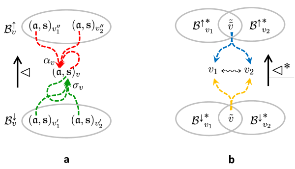
Figure 6: Dependencies for state and activation updates of an observer $v$ (in a) and for coupling between $v_{1}$ and $v_{2}$ (in b). a: The activation and state of an observer $v$ is indicated by $(\mathfrak{a},\mathbf{s})_{v}$. The state $\mathbf{s}$ of $v$ is updated through $\sigma_{v}$, which lets $v$ observe the activations of components $v_{i}^{\prime}$ of $v$ with memory encoded in the previous state $\mathbf{s}$ (green arrows). The activation $\mathfrak{a}$ of $v$ is a direct function of the memory state $\mathbf{s}$ of $v$, top-down controlled by the activations of observers $v^{\prime\prime}_{j}$ in which $v$ is a component (red arrows). b: Two observers $v_{1},v_{2}$ are coupled by shared master when there exists some $\tilde{\tilde{v}}$ of which both are (transitive) components, which means that both are (transitively) controlled by $\tilde{\tilde{v}}$ (blue arrows). They are coupled by shared member if there exists some $\tilde{v}$ which is a (transitive) component of both, such that both $v_{1}$ and $v_{2}$ (transitively) observe $\tilde{v}$ (orange arrows).

Bidirectional, asymmetric vertical interaction through binding.

We thus have a bidirectional influence between observers $v^{\prime}$ versus $v$ when $v^{\prime}\lhd v$. The bottom-up influence given by (1) is cast as an observation relation with memory, while the top-down influence (3) is one of memoryless control, as one might say with a very general interpretation of the word ’control’.

Lateral, symmetric interaction through coupling.

We now turn to the second interaction concept that we want to install in FC models, ’coupling’. Coupling interactions are not explicitly modeled in CM^(m) but result indirectly from the dynamics of (1) and (3). We say that two observers $v_{i},v_{j}$ are coupled by shared masters when they share at least one observer $v_{k}$ that sits higher in the binding hierarchy, that is when $v_{i},v_{j}\lhd^{\ast}v_{k}$. All components $v^{\prime}$ of a compound observer $v$, and their transitive sub-components, are coupled by a shared master, which is $v$. And we say that $v_{i},v_{j}$ are coupled by shared members when they share at least one observer $v_{k}$ that sits lower in the binding hierarchy, that is when $v_{k}\lhd^{\ast}v_{i},v_{j}$. In both cases, the activation dynamics of $v_{i}$ and $v_{j}$ exert some influence on each other through the bidirectional binding interactions along the binding pathways from $v_{i},v_{j}$ to $v_{k}$. We write $v_{i}\leftrightsquigarrow v_{j}$ when $v_{i}$ and $v_{j}$ are coupled by shared masters, or by shared members, or by both. Figure 6b illustrates this.

Mutual dependencies between observers induced by coupling may spread throughout $\mathcal{V}$, indirectly linking observers that have neither shared members nor masters: when $v_{1}\leftrightsquigarrow v_{2}\leftrightsquigarrow\cdots\leftrightsquigarrow v_{n}$, perturbations to the state or activation of $v_{1}$ will affect the state/activation dynamics of $v_{n}$. We write $v_{i}\leftrightsquigarrow^{\ast}v_{j}$ to denote this indirect coupling by transitivity.

In our diagrams of cybernetic computing (Figure 5e-g), observers that are bound in composite observers are indicated by colored subbands, and the coupling interactions by vertical arrows. These diagrams show dynamics in some static architecture — the binding structure does change while time goes on. But, note again that the existence of couplings may be made temporally varying in dynamical architectures.

Analogues of coupling in other models of complex systems.

Analogues of coupling by shared members can be found in many complex systems, when two subsystems co-own or exchange messages or materials generated or located within them. At the most fundamental level, this is witnessed by particle interaction models in theoretical physics, where forces between particles can be modeled as the exchange of force-mediating messager particles G. Jaeger (2021). In some AC parallel programming paradigms and AI ’blackboard models’ of cognitive processing, functions or program modules can interact by having simultaneous read/write access to information in a shared memory region Nii (1986).

Analogues of coupling by shared masters occur ubiquitously in hierarchical control systems (in biological neural motor control or in engineered control systems) when several subsystems receive top-down control input from the same superordinate subsystem. This enables coordinated action of end-effectors, for instance muscles which are co-activated by a central pattern generator in a coordinated motor behavior. In physics, ensembles of particles or other microscale subsystems may statistically build up a ’field’ of some sort in a bottom-up way, which in return organizes large-scale interaction patterns of the microsystems in a top-down direction. Such systems can be modeled with mean-field methods, where the ’field’ is mathematically characterized as a dynamical system constituted by a small number (often even a single) of ’order parameters’. Under suitable conditions, the high-dimensional interaction of microsystems simplifies and can be characterized by the low-dimensional ’field’ dynamics in good approximation. In statistical physics, methods of this kind are central for explaining phase transitions. In synergetics Haken (1983), these methods have been have become generalized and adapted to explain ’self-organization’ in a wide range of complex systems in biology, cognitive science, sociology and economics.

Analysis and design of models is tied to understanding coupling.

In our set-up of models CM^(m), the ’lateral’ coupling between model variables $v$ is not explicitly reflected in the model. Instead, coupling interactions emerge indirectly through information sharing in the binding hierarchy. This is different from the ’lateral’ coupling between state variables $x_{i}$ in ODE systems, which is directly visible in the system equations. One might say that ODE systems are designed around such couplings, and the emergence of hierarchical subsystem nestings must be found out post-hoc by nontrivial analyses. In FC models this is reversed: The hierarchical subsystem structuring is explicitly built into the model by its designer, who starts from a conception of this very structuring. Which variables are indirectly coupled via $\leftrightsquigarrow$ is, on the one hand, easily determined from the written-down model CM^(m) by tracing the transitive member and master relations. However, how these interactions could be best intuitively understood and matched against the underlying physical system PS through its physical model PM, is equally nontrivial as the induction of hierarchical structure in ODE models. Interactions by transitive coupling certainly can lead to decisive, global ’self-organization’ (or disruptive ’self-disorganization’) effects when CM^(m) is executed. A modeler might want to foresee such important effects and directly capture them in CM^(m) by introducing master observers that observe and control them, making such effects explicit in the model from the outset.

The primacy of hierarchical structuring over emergent self-organization phenomena is shared by our FC approach and algorithmic modeling. Classical computer programs and machine models likewise start from a hierarchical organization of data structures and functions. The ultimate global behavior of a computer program, when it is executed, is always open to surprises. Some of them cannot be foreseen by any universal prediction method — the most famous example being the undecidability whether a program, once started, actually will halt or run endlessly without ever producing a result. This brings us back to Turing, who proved this!

Execution of a model.

A model CM^(m) must be ’executable’. This can mean several things to mathematicians, computer scientists, or physicists:

• mathematically deriving how an input signal is transformed to an output signal as time progresses;

• simulating ’runs’ of CM^(m) on a digital computer;

• letting the physical system that is modeled by CM^(m) physically evolve, and while it does that, measure physical observables which are predicted by the model.

When CM^(m) is set up with a static architecture, one would expect that the execution dynamics follows mathematically from the update operators $\sigma_{v}$ and $\alpha_{v}$ and the specific format of temporal progression, to which we alluded by the informal notation $\mathfrak{t}\mapsto\mbox{\sf next-}\mathfrak{t}$. However, local specifications of the mode of progression, which define how an individual observer state is updated (as in Equation (1)), may need to be augmented by rules for the global coordination of states that become updated ’simultaneously’ or ’in parallel’ or in ’threads’ — and what this mathematically means, concretely, is a question that must be answered for any concrete FC modeling formalism. In the digital computing world, a rich repertoire of formal methods has been developed to address concurrency in program execution Aceto . (2007). Rules for coordinating concurrent local dynamics would have to become a part of a model CM^(m), except when the mode of progression simply specifies a global time, like $t\in\mathbb{R}$ in physics or $n\in\mathbb{N}$ in digital signal processing, which is shared by all variables in a model.

Besides a formal regulation of concurrency, further modeling elements need to be added to the concepts that we discussed so far, when it comes to dynamical architectures. In these architectures, the binding structure itself becomes time-dependent. In an intuitive graphical illustration (Figure 7) we collect some of the effects that we foresee in such self-modifying model architectures:

• Observers (and their chronicles) can join (a) and split (b), the latter giving rise to copying operations.

• Observers can terminate their existence or become created (c). This effect might be formalized by the creation / delection of observers during execution; it could also be formally captured by declaring that an observer is ’instantiated’ only when its activation is nonzero — as indicated by the fading-out and fading-in in c.

• Observers may bind into, and unbind from composite observers (d). The central segment (broken orange outline) shows the temporary presence of a compound observer made from two primitive observers and one compound observer, which in turn is a binding of three primitive ones. The compound observers have an activation history of their own, which is not shown in the graphic.

From these basic mechanisms one can obtain more complex effects. For instance, a sub-observer in a compound observer may split, resulting in an event where a compound observer spawns a copy instance of one of its member observers. All of these phenomena must be formally characterized. This can be done through adding structure-changing rules within CM^(m), or (like it is the case for declarative programming languages) as a separate, external set of execution control rules.

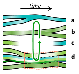
Figure 7: Some effects in self-modifying architectures. Coupling dynamics is symbolized by the circular arrow. Colored bands indicate chronicles of atomic observers, and their varying color intensity indicates varying activation. For explanation see text.

7.3 Observers observe observers across modeling levels

We repeat again that our prime motivation for interpreting variables $v^{(m)}$ as observers is to establish computational models as models of the underlying physical system PS, in a spirit of natural science modeling or engineering. This let us consider the relation between two subsequent models CM^(m) and CM^(m-1) as an observation relation, where the source of what an observer $v^{(m)}$ observes lies in the next-lower model CM^(m-1) (or in the physical model PM for observers $v^{(1)}$ in the machine interface model CM⁽¹⁾). These sources are the observers $v^{(m-1)}$. The level-transiting relations between observers $v^{(m)}$ and $v^{(m-1)}$, marked as ’decoding’ and ’encoding’ in our general schema of computing system modeling (Figure 2), become interpreted in FC as observing and being observed. Iterating these relations down the model hierarchy and further through the physical model connects a higher-level model CM^(m) with its physical substrate.

At the same time we have used the ’observer’ rationale also for the within-model binding relations, which we (semi-)formalized through the state update and activation update operators (1) and (3). To justify this secondary use of the ’observer’ concept we argued that in compilation hierarchies in classical computer programming, the within-program definitions of composite data structures and functions from simpler ones are of the same kind as when a data structure or function, which is a primitive in a higher-level programming language, becomes compiled into a composite structure or process in a program written in a more elementary programming language. The distinction of composition hierarchies within versus between programs effectively blurs when a higher-level programming language admits the direct inclusion of lower-level code. In CS textbook theory the syntax of programming languages is defined by context-free grammars. Such grammars can switch to sub-grammars in their ’parse tree’ representations of computer programs, which provides a single mathematical format for both within- and between-program compositionality.

In our FC proposal, we likewise use the same formal characterization for within- and between-model observations. Consider two models CM^(m) and CM^(m-1). A designer of these two models connects them by declaring observation relations between observers $v^{(m)}$ in CM^(m) and some observees $v_{i}^{(m-1)}$ in CM^(m-1). Within a model we referred to these observation relations as ’binding’. Across two models, we will say that $v^{(m)}$ becomes defined through the $v_{i}^{(m-1)}$ that it observes. We adopt definitions from the previous subsection as follows, assuming possibly different temporal progression modes $\mathfrak{t}^{(m)}$ and $\mathfrak{t}^{(m-1)}$ at the two modeling levels:

• Observers $v^{(m)}$ in CM^(m) are declared by the modeler to be either of type grounded or of type free. The type of $v^{(m)}$ remains fixed throughout the times when $v^{(m)}$ is instantiated in an execution of CM^(m).

• Free observers $v^{(m)}$ do not observe observers in CM^(m-1).

• For a grounded observer $v^{(m)}$, a set $\mathcal{G}_{v^{(m)}}$ of observers $v_{i}^{(m)}$ in CM^(m-1) is declared, called the grounding of $v^{(m)}$. The grounding $\mathcal{G}_{v^{(m)}}$ remains fixed during executions of CM^(m).

• For a grounded $v^{(m)}$, the modeler declares a state update rule, which essentially has the same form as the model-internal state update rule:

  $$\mathbf{s}_{v^{(m)}}(\mbox{\sf next-}\mathfrak{t}^{(m)})=\tilde{\sigma}_{v^{(m)}}\left(\mathbf{s}_{v^{(m)}}(\mathfrak{t}^{(m)}),\left(\mathfrak{a}_{v^{(m-1)}}(\mathfrak{t}^{(m-1)})\right)_{v^{(m-1)}\in\mathcal{G}_{v^{(m)}}}\right).$$ (4)

  This semi-formal schema is incomplete in that it does not explain how the temporal progression $\mathfrak{t}^{(m)}$ synchronizes with $\mathfrak{t}^{(m-1)}$. Additional specifications must be supplied by the modeler for concurrency bonds between $\mathfrak{t}^{(m)}$ and $\mathfrak{t}^{(m-1)}$. The idea in (4) is that $\mathfrak{t}^{(m)}$ and $\mathfrak{t}^{(m-1)}$ are ’simultaneous’. This needs to be worked out together with concrete FC modeling formalisms.

• Our within-model binding relation lets the activation dynamics of $v^{(m)}$ be controlled top-down from master observers (Figure 6a). In contrast, between models CM^(m) and CM^(m-1) there is no top-down control. We thus have no equivalent of (3) here.

We therefore have two hierarchies — the within-model binding hierarchy and the between-model grounding hierarchy — which both originate from the intuition of casting model variables as observers, and whose state update rules mirror each other. This raises the question, what are the deeper reasons for having two such similar hierarchies, and what roles do they play in the modeling game? This question is connected to fundamental issues in scientific modeling and engineering practice at large, and cannot be answered with a single answer. We explore some facets of this theme:

• Model hierarchies in the natural and neurosciences are often conceived as hierarchies of abstraction. When the cognitive reasoning dynamics of a brain is modeled in a classical AI formalism, all detail of neuron-level dynamics is collectivized, averaged, grouped, unified, simplified, etc. — in short, ’abstracted’ (a word whose meaning at first sight seems clear like white light, but upon serious thinking splits into a rainbow spectrum of meanings). Stepping up the abstraction ladder through a model hierarchy, mechanical detail recedes from sight and functional insight comes closer. Information of some sort is lost, and of another sort is created (’information’ being another of these meaning-full words).

  There is a noteworthy difference between model abstraction hierarchies in the natural sciences, and hierarchies of AC programming languages and programs written in them. The latter admit exact two-way translations, while the former do not. A program written in Python can be effectively translated to a program expressed in C, whose I/O functionality is exactly identical. Python is considered higher-level than C, and automated translation engines (compilers) exist. But it would equally be possible to translate C code to equivalent Python code, though this direction will hardly be used in practice.

  Let us take a closer look at translations from C to Python. There are two ways of doing this. The first is the easy one: the ’fine-grained’ data structures and functions of C code are 1-1 recoded in Python. The resulting Python program simulates all the minute operations in the C program. This is straightforward to automate, but it blows up the size of the program and runtime. The second way is much harder and essentially impossible to automate: find a compact equivalent Python program. This means that the modeler has to discover complex patterns within the C code that can be condensed into single Python data structures or commands. This creative, insightful upwards translation is sometimes called ’decompilation’ in the CS world, with the additional connotation that this should be done in a more or less automated fashion. When decompilation is automated, the resulting higher-level code is often obscure and hard to make sense of by humans.

  Summarizing the intuitions and practice of compilation in classical programming: compilation from a higher-level language to a lower-level one is easy and automatic and turns conceptually more intuitive code into more efficient code that is closer to machine mechanics, while de-compilation from a lower-level language to a a conceptually better interpretable version is creative and hard or impossible to automate.

  The modeling hierarchies in the natural sciences are of the second, insightful, creative, bottom-up kind. There is no analogue of mechanical top-down compilation in scientific modeling hierarchies.

  Our FC proposal follows the natural science way of thinking about abstraction. Formulating a higher-level model CM^(m) on the basis of CM^(m-1), and linking it to that lower-level model by observation relations, reflects creative modeling insight. We do not expect that CM^(m) can be distilled automatically from CM^(m-1), nor CM^(m-1) from CM^(m).

• A difference between ’abstraction’ in FC model hierarchies versus model abstraction in the natural sciences lies in the scientific objectives that motivate the modeling efforts in the first place. In the sciences, the objective for creating models on all levels is to gain a deeply organized understanding of the physical system that lies underneath the finest-grained model at the bottom of the modeling hierarchy. In FC modeling, as well as in any cybernetic or algorithmic model hierarchy, the objective of increasing model abstraction is to connect a usecase or task that arises in an real-world task environment (TE in Figure 2) to the physical computing system PS. Each step upwards from some CM^(m-1) to CM^(m) thus should help to ’morph’ the computational model from the physical system model PM toward the task model TM (always referring to Figure 2). In scientific model abstraction, ’more abstract’ means a more globally organized understanding of a physical system PS, while in computational abstraction it means a more task-oriented understanding.

  This distinction between different modeling objectives is however most clear-cut in model hierarchies in physics and chemistry. In biology — in neuroscience especially — the target system may be regarded to have a purpose of its own, which the modeler wants to capture at the abstract high end of the modeling hierarchy. In computational terminology, there might be a ’task’ which the biological system ’wants’ to fulfil, or which it ’should’ optimize. Such a ’task’ might be quite globally stated as ’staying viable in a stochastic and possibly hostile environment’. This leads to modeling efforts geared at revealing robustness properties of biological systems, which is a prime theme in systems biology. In computational neuroscience, the ’task’ of a brain may be formulated in more concrete terms, for instance as enabling the animal to predict the consequences of its actions, or as action planning, or even as being able to use language. To the extent that the overall modeling objective is task-oriented in some way, the nature of ’abstraction’ becomes similar to what we find in modeling computing systems.

• A difference between abstraction in FC model hierarchies versus model abstraction in classical compilation hierarchies is connected to loss of information. Classical programs within a compilation hierarchy are functionally equivalent, while models in FC hierarchies will typically not be functionally equivalent. The higher-level temporal progression mode $\mathfrak{t}^{(m)}$ and the activation model $\mathfrak{a}^{(m)}$ may be coarser in some ways than $\mathfrak{t}^{(m-1)}$ and $\mathfrak{a}^{(m-1)}$. Furthermore, the modeler may simply ignore some of the substructures and subprocesses in CM^(m-1) and only partially exploit CM^(m-1), recruiting and re-interpreting only mechanisms in CM^(m-1) that appear to be useful for the task.

• The distinction between grounded and free observers $v^{(m)}$ is a matter of convenience in modeling practice. The execution of a model CM^(m) must not lead to innovative dynamics that cannot be reduced to the execution dynamics of CM^(m-1). The modeler may decide to define a free observer $v^{(m)}$ only within CM^(m), by declaring it as a compound observer that binds some components $v_{i}^{(m)}$. The level-$m$ observers in ${\mathcal{B}^{\downarrow}}^{\ast}_{v^{(m)}}(\mathfrak{t})$, that is all the members in the component tree underneath $v^{(m)}$, must ultimately be grounded: every subcomponent path $v^{(m)}\rhd_{\mathfrak{t}}v_{1}^{(m)}\rhd_{\mathfrak{t}}v_{2}^{(m)}\rhd_{\mathfrak{t}}\ldots$ must ultimately lead to grounded observers. Thus, an observer $v^{(m)}$ that is declared by the modeler without explicit grounding in CM^(m-1), could also equivalently be declared via grounding through all its grounded (transitive) components.

  This situation is analogue to a common practice in machine learning. In graphical models Jordan (2004) one frequently introduces ’hidden’ variables, which are random variables whose values are not directly observable in the modeled target domain, but whose distributions are ultimately conditioned on observable variables.

• Abstraction from CM^(m-1) to CM^(m) may entail a loss of information through coarsening and omitting subsystems. But at the same time, the creative selection, re-combination and re-interpretation of subprocesses in CM^(m-1), which moves CM^(m) closer to the conceptual framing of the task model TM, can be regarded as adding ’knowledge’ that stems from the modeler’s prior insight in the task conditions. This added influx of modeler’s knowledge can intuitively also be called ’information’, although this sort of information is certainly not Shannon information in the sense of information theory. The mathematical format of this sort of information is unclear, and making it formal will depend on the formal workout of a concrete FC formalism. An analogue is the ’Bayesian prior’ known in Bayesian statistics.

• The commutativity conditions that we pointed out in Section 4 must be satisfied in FC model hierarchies.

• One natural way of abstracting CM^(m-1) to CM^(m) is to

  • set the variables $\mathcal{V}^{(m)}$ in CM^(m) equal to (copies of) the variables in $\mathcal{V}^{(m-1)}$ that are highest-level compounds in CM^(m-1), that is to re-use only the most complex observers from CM^(m-1),

  • and then find suitable temporal progression modes, state representations and activation laws between those compound observers that let the diagrams of CM^(m-1) and CM^(m) commute.

7.4 Some general observations on observations in FC modeling

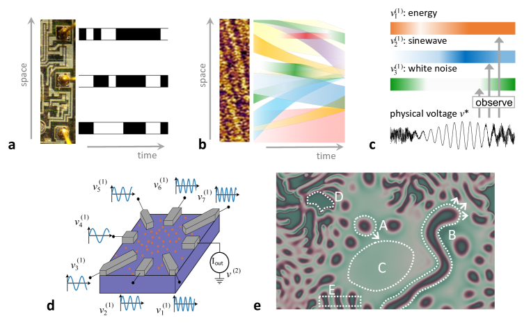
Figure 8: Highlighting some aspects of observers. For explanation see text.

In Figure 8 we illustrate some facts and examples about observations that are pertinent to building model abstraction hierarchies in an FC spirit.

Localizing bit signals (a).

An observer — whether a voltmeter or a human — does not observe the observed physical system at large but focuses on a segment of it. Specifying an observer includes a specification of its source. Often this will boil down to specifying a physical location. The binary bit switching signals in a digital microchip can be picked up at pointlike, non-moving localizations.

Observables can be spatially extended (b).

In physical substrates (microphotography shows the material from Figure 1) one can observe objects or phenomena that are spatially extended, geometrically time-varying, and moving — fields, wave fronts, particles and more. An observer declaration must include means to identify, localize, and track such objects.

There are unlimited ways to define observers (c).

The graphic shows records from three observers $v_{1}^{(1)}$, $v_{2}^{(1)}$, $v_{3}^{(1)}$ that observe the voltage $v^{\ast}$ of an electronic contact point, where here $v^{\ast}$ is a variable in the physical model PM. Their activations (indicated by color intensity) respond to the short-term averaged signal energy, a specific sine frequency response, and the white noise component, respectively. In an FC model there can be an infinity of observers of different quality at every level of modeling abstraction, and even an infinity of observers of different quality that observe the same source.

A complex physical observer (d).

Observers can have internal state and memory, enabling them to integrate and filter information over time. The drawing (adapted from RuizEuleretal20) shows a schematic of a dopant network processing unit (DNPU) Chen . (2020), an unconventional nanoscale device developed in the lab of co-author WvdW. It consists of a doped silicon well which here is contacted by seven input and one output electrode. DNPUs exhibit strongly nonlinear charge transport behaviour between the electrodes. They can implement different computational models, including neural circuits. The drawing shows an experiment where different input voltage signals lead to a nonlinear current response in the output. A neural network was trained to model this highly nonlinear 7-input, 1-output function. Using this model, modular DNPU architectures were mathematically optimized to yield very compact signal processing and pattern recognition systems, including handwritten digit recognition Ruiz Euler . (2021), which were then tested with physical DNPUs.

This neural network model of a DNPU can be formally cast as an observer of the seven inputs $v^{(1)}_{1}-v^{(1)}_{7}$ together. The activation signal $v^{(2)}$ of the trained model output neuron yiels the chronicle of this observer.

Observing spatiotemporal patterns (e).

This graphic (background image created with the fabulous online tool of Sims23) shows a snapshot from an evolving chemical reaction-diffusion system. We might consider as observable phenomena, for example, moving solitons (A), moving and growing filaments (B), neutral ground state areas (C), activated areas (D), periodic patterns (E). Arbitrarily more pattern categories can be defined.

8 Algorithmic models seen as fluent models

Digital computers are physical machines, and our FC proposal aims at modeling general physical computing systems. Thus it should be possible to re-cast the workings of digital or other symbolic-algorithmic machines in the FC modeling framework. How this can be done depends in its details on the specific AC model that one wishes to re-formulate as an FC model. Here we explain in general terms the main steps needed to transform classical AC models into FC models.

The main hurdle is that AC state variables $v_{\mbox{\tiny\sf AC}}^{(m)}$ take arbitrarily nested symbol structures as values, while FC state variables $v_{\mbox{\tiny\sf FC}}^{(m)}$ have ’scalar’ activation values $\mathfrak{a}_{v_{\mbox{\tiny\sf FC}}^{(m)}}$. At low modeling levels CM^(m) close to the physical hardware, by default we think of such activations as non-negative real numbers $a\in\mathbb{R}^{\geq 0}$; at more abstract higher modeling levels we will often want to use reduced-precision versions, like natural numbers or suitably defined fuzzy intervals of $\mathbb{R}^{\geq 0}$. But in any case, an activation value should be in some sense ’one-dimensional’ and not internally structured.

We consider some fixed AC modeling level CM^(m) and will again drop the superscript $\cdot^{(m)}$ for better readability. For simplicity let us assume that the AC model uses global discrete update steps $n\in\mathbb{N}$. Consider the situation that after step $n$, an AC variable $v_{\mbox{\tiny\sf AC}}$ has been assigned the nested symbolic data structure $D$ as its value, that is $v_{\mbox{\tiny\sf AC}}(n)=D$. In order to re-formulate this fact in terms of unstructured scalar activations, we can mirror the compositional structure of $D$ in an analogue compositional binding structure of a composite observer $v_{\mbox{\tiny\sf FC}}$, and encode the symbols at the innermost nesting level in $D$ by what is known as ’one-hot’ encoding in machine learning.

This is best explained with an elementary example. Consider a symbolic term $D=$ 6*2. AC theorists would bring the hierarchical nesting structure of $D$ to the front by drawing its parse tree according to the syntax grammar of the used AC modeling formalism (Figure 9a). This could be done by introducing variables BAT (’binary arithmetic term’), OP (’operator’), ARGS (’arguments’), ARG1 (’first argument’), ARG2 (’second argument’) for the grammatical substructures, and terminal symbols +, * and 0, $\ldots$, 9 for the possible operators and argument values.

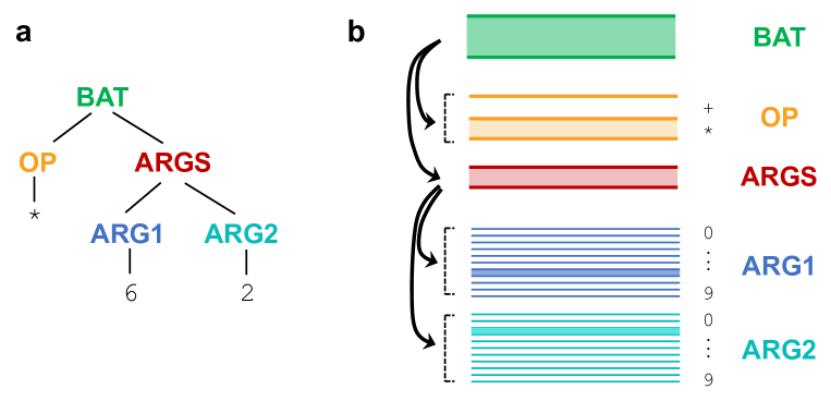
Figure 9: a: Parse tree for the binary arithmetic term 6*2. b: Its re-formulation in an observer binding structure. For explanation see text.

In an FC re-formulation, the grammatical variables BAT, OP, ARGS, ARG1, ARG2 as well as the terminal symbols +, *, 0, $\ldots$, 9 become observers, with a binding structure identical to the parse tree structure (Figure 9b). The top-level observer BAT is bound from two sub-observers OP and ARGS; the observer OP is a compound of two atomic observers + and *; the ARGS observer is obtained by binding together ARG1 with ARG2; and these latter ones are each composites of ten atomic observers 0, $\ldots$, 9.

The fact that the specific value of $v_{\mbox{\tiny\sf AC}}$ at time $n$ is 6*2 (and not, for instance, 3+7) can be encoded, for instance, in the FC version by setting the activation of the * observer to 1 and of + to 0, and similarly setting the activations of 6 and 2 inside ARG1 and ARG2 to 1, while the other atomic digit observers have zero activation. The unit activations are marked in Figure 9b by color filling. The higher-level observers BAT and ARGS also get unit activations. More formally, in the FC version we would use the discrete temporal progression $\mathfrak{t}=n\in\mathbb{N}$ and set $\mathfrak{a}_{\scriptsize\mbox{\sf BAT}}(n)=1$, $\ldots$, $\mathfrak{a}_{{\scriptsize\mbox{\tt 2}}\mbox{\scriptsize-in-}{\scriptsize\mbox{\sf ARG2}}}(n)=1$.

This ’one-hot’ encoding scheme for re-formulating compound AC variable values as 0/1 activation patterns in compound FC observers is not the only option. For instance, one could alternatively encode the 10 different digit values of ARG1 or ARG2 in an AC model by ten different activation levels of atomic observers ARG1 or ARG2 in an FC model.

In an AC computation process, a model variable $v_{\mbox{\tiny\sf AC}}$ need not have a defined value at all times during the computation. In an FC re-modeling, this can be accomodated by setting the activations of the mirror observer $v_{\mbox{\tiny\sf FC}}$ to zero at times $n$ when it has no defined value. Furthermore, new variables can be dynamically created or deleted during an AC computation. This would be mirrored in an FC setting by dynamical model architectures.

Figure 10 illustrates in a schematic way how a sequence of threaded AC operations can be re-cast as a fluent computation with a discrete mode of progression (panel b) or a continuous one (panel c). In the latter case, the operations of the digital clock, which is needed to coordinate the within- and between-thread data transformations steps, can be accomodated by a ’clock observer’ $v_{\mbox{\scriptsize tick}}$, whose activation history is shown in the violet bar on top of the graphic. This observer is blind - it observes no other observers. It is an autonomous activity oscillator. Using continuous time $t\in\mathbb{R}$, its state and activation updates (Equations 1 and 3) reduce to $\dot{\mathbf{s}}_{v_{\mbox{\tiny tick}}}=\sigma_{v_{\mbox{\tiny tick}}}({\mathbf{s}}_{v_{\mbox{\tiny tick}}})$ and $\mathfrak{a}_{v_{\mbox{\tiny tick}}}(t)=\alpha_{v_{\mbox{\tiny tick}}}({\mathbf{s}}_{v_{\mbox{\tiny tick}}}(t))$. The format of the state update law allows the formulation of any desired oscillator dynamics. The clock observer $v_{\mbox{\scriptsize tick}}$ would become a component of every other observer in the model (indicated by vertical green arrows in Figure 10c).

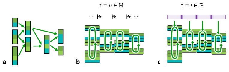
Figure 10: An algorithmic computation (a, extracted from Figure 5) re-cast as a fluent computation in a discrete (b) and a continuous mode of progression (c). The hierarchical sub-structuring of observers, illustrated in Figure 9, is not shown in b and c. For explanation see text.

Of course all of this is only a superficial sketch, which would need to be specified in detail according to the specific formalism that one uses for an FC model.

9 Summary, discussion and outlook

Research in neuromorphic and other unconventional kinds of computing is thriving, but still lacking a unifying theory grounding. We propose to anchor such a theory in three ideas: viewing information processing as a dynamical system (adopted from the cybernetic paradigm), organizing these dynamics in hierarchical binding compounds (adopted from the algorithmic paradigm), and ground theory abstraction in hierarchies of formal observers (following physics).

The core of our FC proposal is to construe formal computational objects as abstract observers of physical phenomena in the material substrate of a computing system. This reverses of Turing’s view. Turing conceived of discrete symbolic structures and their transformations as a model of rational, symbolic reasoning. This perspective makes AC models easily “thinkable” for humans, because there is a pre-established harmony between the reasoning of a well-trained programmer and the structure of computer programs. The downside is that the discrete symbolic structures and discrete-step mechanisms of digital computer programs (or other AC models) must be imposed on the physical hardware. Only hardware systems which are engineered around discrete switching dynamics can serve as physical bases for algorithmic computing. In our reversed perspective, any observable physical phenomenon is a candidate carrier for computing. The downside here is that FC models cannot be directly mapped to rational, discretely rule-based, symbolic human reasoning. But they might turn out to be readily mappable to other modalities of human cognitive processing — associative thinking, sensori-motor perception-action dynamics, continual adaptation and learning, graded concepts and other cognitive phenomena that indeed happen in our brains. A general theory of physical computing — whether it is shaped after our FC proposal or in some other way — should do good service as a mathematical tool for modeling processes in biological brains.

Surely there are many ways how the FC ideas, which at present we can only outline in a schematic manner, can be tied together in mathematical detail. There are a number of nontrivial tasks that must be solved in order to obtain a full mathematical workout, among them the following:

• Define a hierarchally organized systems of temporal progressions $\mathfrak{t}$, presumably starting from the standard continuous timeline model $t\in\mathbb{R}$ used in physical modeling, and leading to the entirely de-materialized progression of successive logical inference steps that is used in the Turing machine model. Similarly, an abstraction hierarchy of activation models $\mathfrak{a}$ must be established.

• Define binding operators for observers. In algorithmic modeling formalisms, the format of all data structures can ultimately be reduced to writing them as trees, or equivalently, nested lists. For an FC formalism one may want to consider other options too, for instance grouping sub-observers in unstructured sets, or declaring weighted connections between them.

• Define mathematical formats for the state update functions $\sigma_{v}$ and activation functions $\alpha_{v}$. These have to agree with the chosen models for temporal progression and activation values. Furthermore, in order to obtain ’executable’ models CM^(m), global coordination mechanisms must be defined, which regulate the interaction of subprocesses. This will likely require the introduction of geometrical space concepts in which observers can be localized.

• In order to specify commuting diagram conditions one needs measures of similarity between two versions of observers and their activations, which are determined by within-level-$m$ transformations and cross-level determination pathways (like the two $x_{2}^{(1)}$ versions in Figure 3).

• In this article we have not started to investigate how in an FC modeling scenario the task model TM (recall Figure 2) should be devised. From a user perspective, many non-digital computing systems will behave quite differently from digital computers. They may not be programmable in the customary sense but need to be trained; they may execute stochastically; they will operate continuously and may not be rebootable or even not re-startable; their output signals may be neither numerical nor symbolic but physical of some sort which needs other mathematical formats to be appropriately captured (for instance through topological objects in dynamical systems or probability distributions H. Jaeger (20211)). The logic formalisms used in AC for task modeling are not immediately suited to capture such aspects, and new mathematical modeling perspectives may have to be found. In the historical development of AC, the problem of formalizing tasks and connecting them to the procedural mechanics of computational models through program verification techniques came into view only after digital computers became widely used. We would expect that developing TM modeling formalisms for FC can likewise be postponed.

All of this together looks somewhat fearsome. However, we have good hopes that we can find the right mathematical abstractions that make the challenge is less daunting and the resulting FC formalism less complex than how it might appear at first sight. The main idea is to express the dynamical effects of state update operators, in a spirit of formal algebra, in terms of changes to the binding structure itself. This line of work has been pursued by H.J. for several years and is making good progress, but we cannot promise a publishable ready-to-use yet.

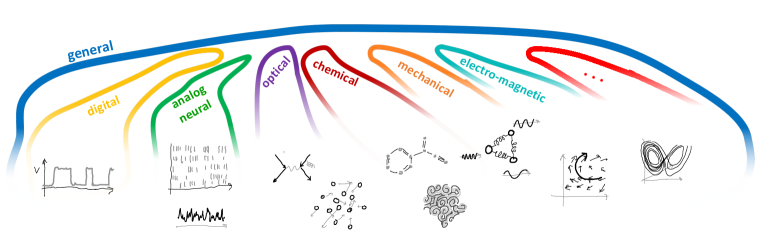
Figure 11: A general theory of physical computing systems would comprise existing theories as special cases.

Let us briefly reflect on what a worked-out general theory of physical computing systems (whether of an FC sort or other) could give us:

Unified terminology:

Researchers who today are using different conceptual framings and terminologies could formulate their insights in the shared scientific language of a GFT.

Model translations:

In each of the currently used modeling frameworks we could identify what is essential for computing, and translate this into other languages and models. A role model for such substance-identifying and substance-preserving formalism translations are the meta-models of universal logic that are developed in theoretical computer science. A readable introduction to this advanced field of mathematical logic is given in Rabe08; Rabe17 gives a recent synopsis. The tools from universal logic allow logicians to identify the essential logical (i.e., proof-enabling) ideas that mathematicians use in their varied subbranches of mathematics (algebra, calculus, probability and all others) and to translate them across different mathematical terminologies, formalisms, and axiomatic frameworks. Similarly, a general theory of physical computing systems may enable us to compare and interrelate computational mechansism that arise from seemingly quite different physical phenomena in different sorts of computational materials (Figure 11).

Physical phenomena translations:

A diversity of nonlinear micro- or nanoscale effects is currently being explored for computational exploits in the materials sciences. At present we do not have conceptual tools (let alone rigorous mathematical definitions) of how to identify, across this sparkling spectrum of physical phenomena, those invariances that are constitutive for computational function. All we can see today is a small number of basic dynamical similarities (like the characterization of hysteretic or oscillatory dynamics), statistical equivalences (like types of phase transitions) or structural-geometrical analogies (like boundary formation or filament growing). But we do not yet understand how such invariances may become coupled into computationally functional complex bundles of mechanisms, and very likely we are still blind to many types of physical phenomenal invariances that are important for general computing functions.

Simulation models:

A worked-out model hierarchy for computing systems should be concrete enough to enable the design of generic simulation tools, runnable on digital computers like all formal models in the natural sciences. These simulations would allow us to experimentally explore generic computational systems that are formulated independent of specific physical substrates or modalities (optical, electronic, mechanic etc.).

General computing as a natural science:

A GFT would enable us to to generate falsifiable hypotheses (testable in generic simulation or specific physical experiments) and predict computational phenomena that have not yet been observed in reality.

Research transfer between natural and engineered systems.

Many formal models that are specializations of a GFT (Figure 11) may be dually applicable to natural and engineered systems. This is clear for analog models of neural systems that are conceived at the interface between computational neuroscience and neuromorphic engineering. There are also digital models of biological neural systems, for instance the classical McCullogh-Pitts model McCulloch  Pitts (1943).

System comparison and classification:

In analogy to the deeply insightful classification system for AC algorithms offered by computational complexity theory Fortnow  Homer (2003), a general theory of physical computing systems could help us to define and compare different sorts of computing systems, classified according to their power and cost. In computational complexity theory different sorts of cost have been defined, like runtime or memory consumption. For general computing systems, new sorts of cost may be identified and formally characterized, for instance relating to energy consumption, physical endurance and replicability, or other criteria which are outside the classical AC perspective but come into view when physical properties of the underlying hardware substrates become essential modeling targets Blakey (2017).

Transcending computing:

Finally, the new formal modeling tools and their underlying conceptual intuitions may extend our scientific methods repertoir to describe and analyse general complex systems which are not primarily seen as computing systems, in particular biological and social systems.

We hope that this article gives useful orientation for theory builders who, like ourselves, are searching for the key to unlock the richness of material physics at large for engineering neuromorphic and other unconventional computing systems.

Acknowledgements H.J. acknowledges financial support from the European Horizon 2020 projects Memory technologies with multi-scale time constants for neuromorphic architectures (grant Nr. 871371) and Post-Digital (grant Nr. 860360). W.G.v.d.W acknowledges financial support from the HYBRAIN project funded by the European Union’s Horizon Europe research and innovation programme under Grant Agreement No 101046878 and the Deutsche Forschungsgemeinschaft (DFG, German Research Foundation) through project 433682494 – SFB 1459. B.N. acknowledges funding from the European Union’s Horizon 2020 ETN programme Materials for Neuromorphic Circuits (MANIC) under the Marie Skłodowska-Curie grant agreement No 861153. Financial support by the Groningen Cognitive Systems and Materials Center (CogniGron) and the Ubbo Emmius Foundation of the University of Groningen is gratefully acknowledged. Finally, we want to thank the reviewers of the short journal version H. Jaeger . (2023) of this arXiv article for their extensive, insightful and constructive feedback. In this long version we tried to accomodate all of their valuable suggestions.

References

- Aceto \BOthers. (\APACyear2007) \APACinsertmetastarAcetoetal07{APACrefauthors}Aceto, L., Ingólfsdóttir, A., Larsen, K\BPBIG.\BCBL \BBA Srba, J. \APACrefYear2007. \APACrefbtitleReactive Systems: Modelling, Specification and Verification Reactive systems: Modelling, specification and verification. \APACaddressPublisherCambridge University Press. \PrintBackRefs\CurrentBib
- Ackley \BOthers. (\APACyear1985) \APACinsertmetastarAckleyetal85{APACrefauthors}Ackley, D\BPBIH., Hinton, G\BPBIE.\BCBL \BBA Sejnowski, T\BPBIJ. \APACrefYearMonthDay1985. \BBOQ\APACrefatitleA Learning Algorithm for Boltzmann Machines A learning algorithm for Boltzmann machines.\BBCQ \APACjournalVolNumPagesCognitive Science9147-169. \PrintBackRefs\CurrentBib
- Adamatzky (\APACyear2015) \APACinsertmetastarAdamatzky15{APACrefauthors}Adamatzky, A. \APACrefYearMonthDay2015. \BBOQ\APACrefatitleSlime mould processors, logic gates and sensors Slime mould processors, logic gates and sensors.\BBCQ \APACjournalVolNumPagesPhilosophical Transactions of the Royal Society A: Mathematical, Physical and Engineering Sciences373204620140216. \PrintBackRefs\CurrentBib
- Adamatzky (\APACyear2017) \APACinsertmetastarAdamatzky17ab{APACrefauthors}Adamatzky, A. (\BED). \APACrefYear2017. \APACrefbtitleAdvances in Unconventional Computing Vol. 1: Theory, and Vol. 2: Prototypes, Models and Algorithms Advances in unconventional computing vol. 1: Theory, and vol. 2: Prototypes, models and algorithms. \APACaddressPublisherSpringer International Publishing AG Switzerland. \PrintBackRefs\CurrentBib
- Adamatzky (\APACyear2018) \APACinsertmetastarAdamatzky18{APACrefauthors}Adamatzky, A. \APACrefYearMonthDay2018. \BBOQ\APACrefatitleTowards fungal computer Towards fungal computer.\BBCQ \APACjournalVolNumPagesInterface Focus820180029. \PrintBackRefs\CurrentBib
- Adolphs (\APACyear2015) \APACinsertmetastarAdolphs15{APACrefauthors}Adolphs, R. \APACrefYearMonthDay2015. \BBOQ\APACrefatitleThe unsolved problems of neuroscience The unsolved problems of neuroscience.\BBCQ \APACjournalVolNumPagesTrends in Cognitive Science194173-175. \PrintBackRefs\CurrentBib
- Albus (\APACyear1993) \APACinsertmetastarAlbus93{APACrefauthors}Albus, J\BPBIS. \APACrefYearMonthDay1993. \BBOQ\APACrefatitleA Reference Model Architecture for Intelligent Systems Design A reference model architecture for intelligent systems design.\BBCQ \BIn P\BPBIJ. Antsaklis \BBA K\BPBIM. Passino (\BEDS), \APACrefbtitleAn Introduction to Intelligent and Autonomous Control An introduction to intelligent and autonomous control (\BPG 27-56). \APACaddressPublisherKluwer Academic Publishers. \PrintBackRefs\CurrentBib
- Andrae \BBA Edler (\APACyear2015) \APACinsertmetastarAndraeEdler15{APACrefauthors}Andrae, A\BPBIS\BPBIG.\BCBT \BBA Edler, T. \APACrefYearMonthDay2015. \BBOQ\APACrefatitleOn Global Electricity Usage of Communication Technology: Trends to 2030 On global electricity usage of communication technology: Trends to 2030.\BBCQ \APACjournalVolNumPagesChallenges6117-157. \PrintBackRefs\CurrentBib
- Angelidis \BOthers. (\APACyear2021) \APACinsertmetastarAngelidisetal21{APACrefauthors}Angelidis, E., Buchholz, E., Arreguit, J., Rougé, A., Stewart, T., von Arnim, A.\BDBLIjspeert, A. \APACrefYearMonthDay2021. \BBOQ\APACrefatitleA spiking central pattern generator for the control of a simulated lamprey robot running on SpiNNaker and Loihi neuromorphic boards A spiking central pattern generator for the control of a simulated lamprey robot running on SpiNNaker and Loihi neuromorphic boards.\BBCQ \APACjournalVolNumPagesNeuromorphic Computing and Engineering11014005. \PrintBackRefs\CurrentBib
- Antoulas \BBA Sorensen (\APACyear2001) \APACinsertmetastarAntoulasSorensen01{APACrefauthors}Antoulas, A\BPBIC.\BCBT \BBA Sorensen, D\BPBIC. \APACrefYearMonthDay2001. \BBOQ\APACrefatitleApproximation of large-scale dynamical systems: an overview Approximation of large-scale dynamical systems: an overview.\BBCQ \APACjournalVolNumPagesInternational Journal of Applied Mathematics and Computer Science1151093-1121. \PrintBackRefs\CurrentBib
- Baddeley (\APACyear2003) \APACinsertmetastarBaddeley03{APACrefauthors}Baddeley, A. \APACrefYearMonthDay2003. \BBOQ\APACrefatitleWorking memory: looking back and looking forward Working memory: looking back and looking forward.\BBCQ \APACjournalVolNumPagesNature Reviews Neuroscience410829-839. \PrintBackRefs\CurrentBib
- Bartlett (\APACyear1932) \APACinsertmetastarBartlett32{APACrefauthors}Bartlett, F\BPBIC. \APACrefYear1932. \APACrefbtitleRemembering: a Study in Experimental and Social Psychology Remembering: a study in experimental and social psychology. \APACaddressPublisherCambridge University Press. \PrintBackRefs\CurrentBib
- Beggs \BBA Timme (\APACyear2012) \APACinsertmetastarBeggsTimme12{APACrefauthors}Beggs, J\BPBIM.\BCBT \BBA Timme, N. \APACrefYearMonthDay2012. \BBOQ\APACrefatitleBeing critical of criticality in the brain Being critical of criticality in the brain.\BBCQ \APACjournalVolNumPagesFrontiers in Physiology3article 00163. \PrintBackRefs\CurrentBib
- beim Graben (\APACyear2006) \APACinsertmetastarbeimGraben06{APACrefauthors}beim Graben, P. \APACrefYearMonthDay2006. \BBOQ\APACrefatitlePragmatic Information in Dynamic Semantics Pragmatic information in dynamic semantics.\BBCQ \APACjournalVolNumPagesMind and Matter42169-193. \PrintBackRefs\CurrentBib
- Bekolay \BOthers. (\APACyear2014) \APACinsertmetastarBekolayetal14{APACrefauthors}Bekolay, J., T.and Bergstra, Hunsberger, E., DeWolf, T., Stewart, T\BPBIC., Rasmussen, D., Choo, X.\BDBLEliasmith, C. \APACrefYearMonthDay2014. \BBOQ\APACrefatitleNengo: a Python tool for building large-scale functional brain models Nengo: a Python tool for building large-scale functional brain models.\BBCQ \APACjournalVolNumPagesFrontiers in Neuroinformatics7article 481-13. \PrintBackRefs\CurrentBib
- Besold \BOthers. (\APACyear2017) \APACinsertmetastarBesoldetal17{APACrefauthors}Besold, T., d’Avila Garcez, A., Bader, S., Bowman, H., Domingos, P., Hitzler, P.\BDBLZaverucha, G. \APACrefYearMonthDay2017. \APACrefbtitleNeural-Symbolic Learning and Reasoning: A Survey and Interpretation. Neural-symbolic learning and reasoning: A survey and interpretation. \APACrefnotePreprint at https://arxiv.org/pdf/1711.03902 \PrintBackRefs\CurrentBib
- Bickerton \BBA Szathmáry (\APACyear2009) \APACinsertmetastarBickertonSzathmary09{APACrefauthors}Bickerton, D.\BCBT \BBA Szathmáry, E. (\BEDS). \APACrefYear2009. \APACrefbtitleBiological Foundations and Origin of Syntax Biological foundations and origin of syntax. \APACaddressPublisherMIT Press (Strüngmann Forum Reports). \PrintBackRefs\CurrentBib
- Blakey (\APACyear2017) \APACinsertmetastarBlakey17{APACrefauthors}Blakey, E. \APACrefYearMonthDay2017. \BBOQ\APACrefatitleUnconventional Computers and Unconventional Complexity Measures Unconventional computers and unconventional complexity measures.\BBCQ \BIn A. Adamatzky (\BED), \APACrefbtitleAdvances in Unconventional Computing Vol. 1: Theory Advances in unconventional computing vol. 1: Theory (\BPG 165-182). \APACaddressPublisherSpringer. \PrintBackRefs\CurrentBib
- Blum \BOthers. (\APACyear1989) \APACinsertmetastarBlumShubSmale89{APACrefauthors}Blum, L., Shub, M.\BCBL \BBA Smale, S. \APACrefYearMonthDay1989. \BBOQ\APACrefatitleOn a theory of computation and complexity over the real numbers: NP-completeness, recursive functions and universal machines On a theory of computation and complexity over the real numbers: NP-completeness, recursive functions and universal machines.\BBCQ \APACjournalVolNumPagesBulletin of the American Mathematical Society2111-46. \PrintBackRefs\CurrentBib
- Bose \BOthers. (\APACyear2015) \APACinsertmetastarBoseetal15{APACrefauthors}Bose, S\BPBIK., Lawrence, C\BPBIP., Liu, Z., Makarenko, K\BPBIS., van Damme, R\BPBIM., Broersma, H\BPBIJ.\BCBL \BBA van der Wiel, W\BPBIG. \APACrefYearMonthDay2015. \BBOQ\APACrefatitleEvolution of a designless nanoparticle network into reconfigurable Boolean logic Evolution of a designless nanoparticle network into reconfigurable Boolean logic.\BBCQ \APACjournalVolNumPagesNature Nanotechnology10121048-1052. \PrintBackRefs\CurrentBib
- Bournez \BBA Pouly (\APACyear2021) \APACinsertmetastarBournezPouly21{APACrefauthors}Bournez, O.\BCBT \BBA Pouly, A. \APACrefYearMonthDay2021. \BBOQ\APACrefatitleA Survey on Analog Models of Computation A survey on analog models of computation.\BBCQ \BIn V. Brattka \BBA P. Hertling (\BEDS), \APACrefbtitleHandbook of Computability and Complexity in Analysis Handbook of computability and complexity in analysis (\BPG 173-226). \APACaddressPublisherSpringer, Cham. \PrintBackRefs\CurrentBib
- Bradie (\APACyear1986) \APACinsertmetastarBradie86{APACrefauthors}Bradie, M. \APACrefYearMonthDay1986. \BBOQ\APACrefatitleAssessing evolutionary epistemology Assessing evolutionary epistemology.\BBCQ \APACjournalVolNumPagesBiology and Philosophy14401-459. \PrintBackRefs\CurrentBib
- Brenner \BOthers. (\APACyear1986) \APACinsertmetastarBrennerHuangStreibl86{APACrefauthors}Brenner, K\BPBIH., Huang, A.\BCBL \BBA Streibl, N. \APACrefYearMonthDay1986. \BBOQ\APACrefatitleDigital optical computing with symbolic substitution Digital optical computing with symbolic substitution.\BBCQ \APACjournalVolNumPagesApplied Optics25183054-3060. \PrintBackRefs\CurrentBib
- Brooks (\APACyear1995) \APACinsertmetastarBrooks91a{APACrefauthors}Brooks, R\BPBIA. \APACrefYearMonthDay1995. \BBOQ\APACrefatitleIntelligence without Reason Intelligence without reason.\BBCQ \BIn L. Steels \BBA R\BPBIA. Brooks (\BEDS), \APACrefbtitleThe Artificial Life Route to Artificial Intelligence The artificial life route to artificial intelligence (\BPG 25-81). \APACaddressPublisherRoutledge. \APACrefnotereprint of a 1991 techreport, MIT A.I. Memo 1293 \PrintBackRefs\CurrentBib
- Cardelli (\APACyear2005) \APACinsertmetastarCardelli05{APACrefauthors}Cardelli, L. \APACrefYearMonthDay2005. \BBOQ\APACrefatitleBrane calculi: Interactions of biological membranes Brane calculi: Interactions of biological membranes.\BBCQ \BIn \APACrefbtitleProc. of Computational Methods in Systems Biology: International Conference (CMSB 2004), Revised Selected Papers Proc. of computational methods in systems biology: International conference (cmsb 2004), revised selected papers (\BPG 257-278). \APACaddressPublisherSpringer Berlin Heidelberg. \PrintBackRefs\CurrentBib
- Chen \BOthers. (\APACyear2020) \APACinsertmetastarChenetal20{APACrefauthors}Chen, T., van Gelder, J., van de Ven, B., Amitonov, S., de Wilde, B., Ruiz Euler, H\BHBIC.\BDBLvan der Wiel, W\BPBIG. \APACrefYearMonthDay2020. \BBOQ\APACrefatitleClassification with a disordered dopant-atom network in silicon Classification with a disordered dopant-atom network in silicon.\BBCQ \APACjournalVolNumPagesNature577341-345. \PrintBackRefs\CurrentBib
- Chialvo (\APACyear2010) \APACinsertmetastarChialvo10{APACrefauthors}Chialvo, D\BPBIR. \APACrefYearMonthDay2010. \BBOQ\APACrefatitleEmergent complex neural dynamics Emergent complex neural dynamics.\BBCQ \APACjournalVolNumPagesNature Physics610744-750. \PrintBackRefs\CurrentBib
- Chu (\APACyear2016) \APACinsertmetastarMITNews19{APACrefauthors}Chu, J. \APACrefYearMonthDay2016. \APACrefbtitleTESS discovers its first earth-sized planet. TESS discovers its first earth-sized planet. \APACrefnoteOnline press release from MIT, accessed: October 2022. https://news.mit.edu/2019/tess-discovers-first-earth-sized-planet-0416 \PrintBackRefs\CurrentBib
- Clark (\APACyear2013) \APACinsertmetastarClark13{APACrefauthors}Clark, A. \APACrefYearMonthDay2013. \BBOQ\APACrefatitleWhatever Next? Predictive Brains, Situated Agents, and the Future of Cognitive Science. Whatever next? Predictive brains, situated agents, and the future of cognitive science.\BBCQ \APACjournalVolNumPagesBehavioral and Brain Sciences3631-86. \PrintBackRefs\CurrentBib
- Copeland (\APACyear2002) \APACinsertmetastarCopeland02{APACrefauthors}Copeland, B\BPBIJ. \APACrefYearMonthDay2002. \BBOQ\APACrefatitleHypercomputation Hypercomputation.\BBCQ \APACjournalVolNumPagesMinds and Machines124461-502. \PrintBackRefs\CurrentBib
- Coulombe \BOthers. (\APACyear2017) \APACinsertmetastarCoulombeetal17{APACrefauthors}Coulombe, J\BPBIC., York, M\BPBIC\BPBIA.\BCBL \BBA Sylvestre, J. \APACrefYearMonthDay2017. \BBOQ\APACrefatitleComputing with networks of nonlinear mechanical oscillators Computing with networks of nonlinear mechanical oscillators.\BBCQ \APACjournalVolNumPagesPLOS One126. \PrintBackRefs\CurrentBib
- Cover \BBA Thomas (\APACyear2006) \APACinsertmetastarCoverThomas06{APACrefauthors}Cover, T\BPBIM.\BCBT \BBA Thomas, J\BPBIA. \APACrefYear2006. \APACrefbtitleElements of Information Theory, Second Edition Elements of information theory, second edition. \APACaddressPublisherWiley Interscience. \PrintBackRefs\CurrentBib
- Cruse \BOthers. (\APACyear2013) \APACinsertmetastarCruseDeanRitter13{APACrefauthors}Cruse, H., Dean, J.\BCBL \BBA Ritter, H. (\BEDS). \APACrefYear2013. \APACrefbtitlePrerational Intelligence: Adaptive Behavior and Intelligent Systems Without Symbols and Logic (3 volumes) Prerational intelligence: Adaptive behavior and intelligent systems without symbols and logic (3 volumes). \APACaddressPublisherSpringer Science & Business Media. \PrintBackRefs\CurrentBib
- Diesmann \BOthers. (\APACyear1999) \APACinsertmetastarDiesmannetal99{APACrefauthors}Diesmann, M., Gewaltig, M\BHBIO.\BCBL \BBA Aertsen, A. \APACrefYearMonthDay1999. \BBOQ\APACrefatitleStable propagation of synchronous spiking in cortical neural networks Stable propagation of synchronous spiking in cortical neural networks.\BBCQ \APACjournalVolNumPagesNature402529-533. \PrintBackRefs\CurrentBib
- Dommer \BOthers. (\APACyear2021) \APACinsertmetastarDommeretal21{APACrefauthors}Dommer, A., Casalino, L., Kearns, F., Rosenfeld, M., Wauer, N., Ahn, S\BHBIH.\BDBLAmaro, R. \APACrefYearMonthDay2021. \APACrefbtitle#COVIDisAirborne: AI-Enabled Multiscale Computational Microscopy of Delta SARS-CoV-2 in a Respiratory Aerosol #COVIDisairborne: AI-enabled multiscale computational microscopy of Delta SARS-CoV-2 in a respiratory aerosol \APACbVolEdTRbioRxiv report https://www.biorxiv.org/content/10.1101/2021.11.12.468428v1. \APACaddressInstitutionCold Spring Harbor Laboratory. \PrintBackRefs\CurrentBib
- Dorigo \BBA Gambardella (\APACyear1997) \APACinsertmetastarDorigoGambardella97{APACrefauthors}Dorigo, M.\BCBT \BBA Gambardella, L\BPBIM. \APACrefYearMonthDay1997. \BBOQ\APACrefatitleAnt colony system: a cooperative learning approach to the traveling salesman problem Ant colony system: a cooperative learning approach to the traveling salesman problem.\BBCQ \APACjournalVolNumPagesIEEE Transactions on Evolutionary Computation1153-66. \PrintBackRefs\CurrentBib
- Doty (\APACyear2012) \APACinsertmetastarDoty12{APACrefauthors}Doty, D. \APACrefYearMonthDay2012. \BBOQ\APACrefatitleTheory of algorithmic self-assembly Theory of algorithmic self-assembly.\BBCQ \APACjournalVolNumPagesCommunications of the ACM551278-88. \PrintBackRefs\CurrentBib
- Drescher (\APACyear1991) \APACinsertmetastarDrescher91{APACrefauthors}Drescher, G\BPBIL. \APACrefYear1991. \APACrefbtitleMade-up Minds: A Constructivist Approach to Artificial Intelligence Made-up minds: A constructivist approach to artificial intelligence. \APACaddressPublisherMIT Press, Cambridge, Mass. \PrintBackRefs\CurrentBib
- Dubcek \BOthers. (\APACyear2021) \APACinsertmetastarDubceketal21{APACrefauthors}Dubcek, T., Moreno-Garcia, D., Haag, T., Thomsen, H\BPBIR., Becker, T\BPBIS., Bärlocher, C.\BDBLRobertsson, J\BPBIO. \APACrefYearMonthDay2021. \APACrefbtitleBinary classification of spoken words with passive elastic metastructures. Binary classification of spoken words with passive elastic metastructures. \APACrefnotePreprint at https://arxiv.org/abs/2111.08503 \PrintBackRefs\CurrentBib
- Durstewitz \BOthers. (\APACyear2000) \APACinsertmetastarDurstewitzetal00{APACrefauthors}Durstewitz, D., Seamans, J\BPBIK.\BCBL \BBA Sejnowski, T\BPBIJ. \APACrefYearMonthDay2000. \BBOQ\APACrefatitleNeurocomputational models of working memory Neurocomputational models of working memory.\BBCQ \APACjournalVolNumPagesNature Neuroscience31184-91. \PrintBackRefs\CurrentBib
- Ebert (\APACyear2018) \APACinsertmetastarEbert18{APACrefauthors}Ebert, C. \APACrefYearMonthDay2018. \BBOQ\APACrefatitle50 Years of Software Engineering: Progress and Perils 50 years of software engineering: Progress and perils.\BBCQ \APACjournalVolNumPagesIEEE Software35594-101. \PrintBackRefs\CurrentBib
- Eco (\APACyear1979) \APACinsertmetastarEco79{APACrefauthors}Eco, U. \APACrefYear1979. \APACrefbtitleA Theory of Semiotics A theory of semiotics. \APACaddressPublisherIndiana University Press. \PrintBackRefs\CurrentBib
- Eliasmith \BOthers. (\APACyear2012) \APACinsertmetastarEliasmithetal12{APACrefauthors}Eliasmith, C., C., S\BPBIT., X., C., T., B., DeWolf T., T\BPBIY.\BCBL \BBA Rasmussen, D. \APACrefYearMonthDay2012. \BBOQ\APACrefatitleA large-scale model of the functioning brain A large-scale model of the functioning brain.\BBCQ \APACjournalVolNumPagesScience33861111202-1205. \PrintBackRefs\CurrentBib
- Endrullis \BOthers. (\APACyear2019) \APACinsertmetastarEndrullisetal20{APACrefauthors}Endrullis, J., Klop, J\BPBIW.\BCBL \BBA Bakhshi, R. \APACrefYearMonthDay2019. \BBOQ\APACrefatitleTransducer degrees: atoms, infima and suprema Transducer degrees: atoms, infima and suprema.\BBCQ \APACjournalVolNumPagesActa Informatica573-5727-758. \PrintBackRefs\CurrentBib
- Ermentrout (\APACyear1992) \APACinsertmetastarErmentrout92{APACrefauthors}Ermentrout, B. \APACrefYearMonthDay1992. \BBOQ\APACrefatitleComplex dynamics in winner-take-all neural nets with slow inhibition Complex dynamics in winner-take-all neural nets with slow inhibition.\BBCQ \APACjournalVolNumPagesNeural Networks53415-431. \PrintBackRefs\CurrentBib
- European Commission Author Collective (\APACyear2009) \APACinsertmetastarEuropeanCommission09{APACrefauthors}European Commission Author Collective. \APACrefYearMonthDay2009. \APACrefbtitleUnconventional formalisms for computation: Expert Consultation Workshop Unconventional formalisms for computation: Expert consultation workshop \APACbVolEdTRWorkshop report. \APACaddressInstitutionEuropean Commission. \APACrefnotePreprint at https://cordis.europa.eu/pub/fp7/ict/docs/fet-proactive/shapefetip-wp2011-12-05_en.pdf \PrintBackRefs\CurrentBib
- Everhardt \BOthers. (\APACyear2019) \APACinsertmetastarEverhardt2019{APACrefauthors}Everhardt, A\BPBIS., Damerio, S., Zorn, J\BPBIA., Zhou, S., Domingo, N., Catalan, G.\BDBLNoheda, B. \APACrefYearMonthDay2019Aug. \BBOQ\APACrefatitlePeriodicity-Doubling Cascades: Direct Observation in Ferroelastic Materials Periodicity-doubling cascades: Direct observation in ferroelastic materials.\BBCQ \APACjournalVolNumPagesPhysical Review Letters123087603. \PrintBackRefs\CurrentBib
- Everhardt \BOthers. (\APACyear2020) \APACinsertmetastarEverhardt2020{APACrefauthors}Everhardt, A\BPBIS., Denneulin, T., Grünebohm, A., Shao, Y\BHBIT., Ondrejkovic, P., Zhou, S.\BDBLNoheda, B. \APACrefYearMonthDay2020. \BBOQ\APACrefatitleTemperature-independent giant dielectric response in transitional BaTiO3 thin films Temperature-independent giant dielectric response in transitional BaTiO3 thin films.\BBCQ \APACjournalVolNumPagesApplied Physics Review71011402. \PrintBackRefs\CurrentBib
- Fedor \BOthers. (\APACyear2009) \APACinsertmetastarFedorIttzesSzathmary09{APACrefauthors}Fedor, A., Ittzés, P.\BCBL \BBA Szathmáry, E. \APACrefYearMonthDay2009. \BBOQ\APACrefatitleThe biological background of syntax evolution The biological background of syntax evolution.\BBCQ \BIn D. Bickerton \BBA E. Szathmáry (\BEDS), \APACrefbtitleBiological Foundations and Origin of Syntax Biological foundations and origin of syntax (\BPG 15-39). \APACaddressPublisherMIT Press. \PrintBackRefs\CurrentBib
- Feigenbaum (\APACyear1977) \APACinsertmetastarFeigenbaum77{APACrefauthors}Feigenbaum, E. \APACrefYearMonthDay1977. \BBOQ\APACrefatitleThe art of artificial intelligence: themes and case-studies of knowledge engineering The art of artificial intelligence: themes and case-studies of knowledge engineering.\BBCQ \BIn \APACrefbtitleProceedings of IJCAI-77, vol. 2 Proceedings of IJCAI-77, vol. 2 (\BPG 1014-1029). \PrintBackRefs\CurrentBib
- Forbus (\APACyear1988) \APACinsertmetastarForbus88{APACrefauthors}Forbus, K\BPBID. \APACrefYearMonthDay1988. \BBOQ\APACrefatitleQualitative physics: past, present and future Qualitative physics: past, present and future.\BBCQ \BIn \APACrefbtitleExploring Artificial Intelligence: Survey Talks from the National Conferences on Artificial Intelligence Exploring artificial intelligence: Survey talks from the national conferences on artificial intelligence (\BPG 239-296). \APACaddressPublisherMorgan Kaufmann. \PrintBackRefs\CurrentBib
- Forrest (\APACyear1990) \APACinsertmetastarForrest1990a{APACrefauthors}Forrest, S. \APACrefYearMonthDay1990. \BBOQ\APACrefatitleEmergent computation: self-organizing, collective, and cooperative phenomena in natural and artificial computing networks Emergent computation: self-organizing, collective, and cooperative phenomena in natural and artificial computing networks.\BBCQ \APACjournalVolNumPagesPhysica D421-11. \PrintBackRefs\CurrentBib
- Fortnow \BBA Homer (\APACyear2003) \APACinsertmetastarFortnowHomer03{APACrefauthors}Fortnow, L.\BCBT \BBA Homer, S. \APACrefYearMonthDay2003. \BBOQ\APACrefatitleA short history of computational complexity A short history of computational complexity.\BBCQ \APACjournalVolNumPagesBulletin of the EATCS8012003. \PrintBackRefs\CurrentBib
- Fredkin (\APACyear2013) \APACinsertmetastarFredkin13{APACrefauthors}Fredkin, E. \APACrefYearMonthDay2013. \BBOQ\APACrefatitleDiscrete Theoretical Processes (DTP) Discrete theoretical processes (DTP).\BBCQ \BIn H. Zenil (\BED), \APACrefbtitleA Computable Universe: Understanding and exploring Nature as computation A computable universe: Understanding and exploring nature as computation (\BPG 365-380). \APACaddressPublisherWorld Scientific. \PrintBackRefs\CurrentBib
- Freiberger \BOthers. (\APACyear2017) \APACinsertmetastarFreibergeretal17{APACrefauthors}Freiberger, M., Katumba, A., Bienstman, P.\BCBL \BBA Dambre, J. \APACrefYearMonthDay2017. \BBOQ\APACrefatitleOn-chip passive photonic reservoir computing with integrated optical readout On-chip passive photonic reservoir computing with integrated optical readout.\BBCQ \BIn \APACrefbtitleProc. IEEE International Conference on Rebooting Computing (ICRC2017) Proc. ieee international conference on rebooting computing (icrc2017) (\BPG 255-258). \PrintBackRefs\CurrentBib
- Friston (\APACyear2010) \APACinsertmetastarFriston10{APACrefauthors}Friston, K. \APACrefYearMonthDay2010. \BBOQ\APACrefatitleThe free-energy principle: a unified brain theory? The free-energy principle: a unified brain theory?\BBCQ \APACjournalVolNumPagesNature Reviews Neuroscience112127-138. \PrintBackRefs\CurrentBib
- Fusi \BBA Wang (\APACyear2016) \APACinsertmetastarFusiWang16{APACrefauthors}Fusi, S.\BCBT \BBA Wang, X\BHBIJ. \APACrefYearMonthDay2016. \BBOQ\APACrefatitleShort-term, long-term, and working memory Short-term, long-term, and working memory.\BBCQ \BIn M. Arbib \BBA J. Bonaiuto (\BEDS), \APACrefbtitleFrom Neuron to Cognition via Computational Neuroscience From neuron to cognition via computational neuroscience (\BPG 319-344). \APACaddressPublisherMIT Press. \PrintBackRefs\CurrentBib
- Gallego \BOthers. (\APACyear2020) \APACinsertmetastarGallegoetal20{APACrefauthors}Gallego, J\BPBIA., Perich, M\BPBIG., Chowdhury, R\BPBIH., Solla, S\BPBIA.\BCBL \BBA Miller, L\BPBIE. \APACrefYearMonthDay2020. \BBOQ\APACrefatitleLong-term stability of cortical population dynamics underlying consistent behavior Long-term stability of cortical population dynamics underlying consistent behavior.\BBCQ \APACjournalVolNumPagesNature Neuroscience232260-270. \PrintBackRefs\CurrentBib
- Gedeon \BBA Arathorn (\APACyear2007) \APACinsertmetastarGedeonArathorn07{APACrefauthors}Gedeon, T.\BCBT \BBA Arathorn, D. \APACrefYearMonthDay2007. \BBOQ\APACrefatitleConvergence of Map Seeking Circuits Convergence of map seeking circuits.\BBCQ \APACjournalVolNumPagesJournal of Mathematical Imaging and Vision29235-248. \PrintBackRefs\CurrentBib
- Gerstner \BOthers. (\APACyear2012) \APACinsertmetastarGerstneretal12{APACrefauthors}Gerstner, W., Sprekeler, H.\BCBL \BBA Deco, D. \APACrefYearMonthDay2012. \BBOQ\APACrefatitleTheory and Simulation in Neuroscience Theory and simulation in neuroscience.\BBCQ \APACjournalVolNumPagesScience3385 Oct60-65. \PrintBackRefs\CurrentBib
- Geuvers \BOthers. (\APACyear2010) \APACinsertmetastarGeuversetal10{APACrefauthors}Geuvers, H., Koprowski, A., Synek, D.\BCBL \BBA van der Weegen, E. \APACrefYearMonthDay2010. \BBOQ\APACrefatitleAutomated machine-checked hybrid system safety proofs Automated machine-checked hybrid system safety proofs.\BBCQ \BIn \APACrefbtitleProc. Int. Conf. on Interactive Theorem Proving Proc. int. conf. on interactive theorem proving (\BPG 259-274). \APACaddressPublisherSpringer. \PrintBackRefs\CurrentBib
- Gonon \BOthers. (\APACyear2020) \APACinsertmetastarGononGrigoryevaOrtega20a{APACrefauthors}Gonon, L., Grigoryeva, L.\BCBL \BBA Ortega, J\BHBIP. \APACrefYearMonthDay2020. \BBOQ\APACrefatitleMemory and forecasting capacities of nonlinear recurrent networks Memory and forecasting capacities of nonlinear recurrent networks.\BBCQ \APACjournalVolNumPagesPhysica D414December 15132721. \PrintBackRefs\CurrentBib
- Graves \BOthers. (\APACyear2016) \APACinsertmetastarGravesetal16{APACrefauthors}Graves, A., Wayne, G., Reynolds, M., Harley, T., Danihelka, I., Grabska-Barwińska, A.\BDBLHassabis, D. \APACrefYearMonthDay2016. \BBOQ\APACrefatitleHybrid computing using a neural network with dynamic external memory Hybrid computing using a neural network with dynamic external memory.\BBCQ \APACjournalVolNumPagesNature7626471-476. \PrintBackRefs\CurrentBib
- Greenfield (\APACyear1991) \APACinsertmetastarGreenfield91{APACrefauthors}Greenfield, P. \APACrefYearMonthDay1991. \BBOQ\APACrefatitleLanguage, tools and brain: The ontogeny and phylogeny of hierarchically organized sequential behavior Language, tools and brain: The ontogeny and phylogeny of hierarchically organized sequential behavior.\BBCQ \APACjournalVolNumPagesBehavioral and Brain Sciences14531-595. \PrintBackRefs\CurrentBib
- Grigoryeva \BBA Ortega (\APACyear2018\APACexlab\BCnt1) \APACinsertmetastarGrigoryevaOrtega18a{APACrefauthors}Grigoryeva, L.\BCBT \BBA Ortega, J\BHBIP. \APACrefYearMonthDay2018\BCnt1. \BBOQ\APACrefatitleEcho state networks are universal Echo state networks are universal.\BBCQ \APACjournalVolNumPagesNeural Networks10812495-508. \PrintBackRefs\CurrentBib
- Grigoryeva \BBA Ortega (\APACyear2018\APACexlab\BCnt2) \APACinsertmetastarGrigoryevaOrtega18{APACrefauthors}Grigoryeva, L.\BCBT \BBA Ortega, J\BHBIP. \APACrefYearMonthDay2018\BCnt2. \BBOQ\APACrefatitleUniversal discrete-time reservoir computers with stochastic inputs and linear readouts using non-homogeneous state-affine systems Universal discrete-time reservoir computers with stochastic inputs and linear readouts using non-homogeneous state-affine systems.\BBCQ \APACjournalVolNumPagesJournal of Machine Learning Research191892-931. \PrintBackRefs\CurrentBib
- Grollier \BOthers. (\APACyear2020) \APACinsertmetastarGrollieretal20{APACrefauthors}Grollier, J., Querlioz, D., Camsari, K\BPBIJ., Everschor-Sitte, K., Fukami, S.\BCBL \BBA Stiles, M\BPBID. \APACrefYearMonthDay2020. \BBOQ\APACrefatitleNeuromorphic spintronics Neuromorphic spintronics.\BBCQ \APACjournalVolNumPagesNature Electronics37360-370. \PrintBackRefs\CurrentBib
- Gros (\APACyear2009) \APACinsertmetastarGros09{APACrefauthors}Gros, C. \APACrefYearMonthDay2009. \BBOQ\APACrefatitleCognitive computation with autonomously active neural networks: an emerging field Cognitive computation with autonomously active neural networks: an emerging field.\BBCQ \APACjournalVolNumPagesCognitive Computation177-90. \PrintBackRefs\CurrentBib
- Haken (\APACyear1983) \APACinsertmetastarHaken83{APACrefauthors}Haken, H. \APACrefYear1983. \APACrefbtitleAdvanced Synergetics - Instability Hierarchies of Self-Organizing Systems and Devices Advanced synergetics - instability hierarchies of self-organizing systems and devices (\BVOL 20). \APACaddressPublisherSpringer, Berlin/Heidelberg. \PrintBackRefs\CurrentBib
- Haken (\APACyear2008) \APACinsertmetastarHaken08{APACrefauthors}Haken, H. \APACrefYearMonthDay2008. \BBOQ\APACrefatitleSelf-organization Self-organization.\BBCQ \APACjournalVolNumPagesScholarpedia381401. \APACrefnoterevision #139276, retrieved March 2023 \PrintBackRefs\CurrentBib
- Harnad (\APACyear1994) \APACinsertmetastarHarnad94{APACrefauthors}Harnad, S. \APACrefYearMonthDay1994. \BBOQ\APACrefatitleWhat is computation (and is cognition that)? — Preface to special journal issue What is computation (and is cognition that)? — preface to special journal issue.\BBCQ \APACjournalVolNumPagesMinds and Machines44377-378. \PrintBackRefs\CurrentBib
- He \BOthers. (\APACyear2019) \APACinsertmetastarHeetal19{APACrefauthors}He, X., Liu, T., Hadaeghi, F.\BCBL \BBA Jaeger, H. \APACrefYearMonthDay2019. \BBOQ\APACrefatitleReservoir Transfer on Analog Neuromorphic Hardware Reservoir transfer on analog neuromorphic hardware.\BBCQ \BIn \APACrefbtitleProc. 9th Int. IEEE/EMBS Conf. on Neural Engineering Proc. 9th int. ieee/embs conf. on neural engineering (\BPG 1234-1238). \PrintBackRefs\CurrentBib
- Hens \BOthers. (\APACyear2019) \APACinsertmetastarHensetal19{APACrefauthors}Hens, C., Harush, U., Haber, S., Cohen, R.\BCBL \BBA Barzel, B. \APACrefYearMonthDay2019. \BBOQ\APACrefatitleSpatiotemporal signal propagation in complex networks Spatiotemporal signal propagation in complex networks.\BBCQ \APACjournalVolNumPagesNature Physics15403-412. \PrintBackRefs\CurrentBib
- Hinton \BBA Salakuthdinov (\APACyear2006) \APACinsertmetastarHintonSalakhutdinov06{APACrefauthors}Hinton, G\BPBIE.\BCBT \BBA Salakuthdinov, R\BPBIR. \APACrefYearMonthDay2006. \BBOQ\APACrefatitleReducing the Dimensionality of Data with Neural Networks Reducing the dimensionality of data with neural networks.\BBCQ \APACjournalVolNumPagesScience313July 28504-507. \PrintBackRefs\CurrentBib
- Hodgkin \BBA Huxley (\APACyear1952) \APACinsertmetastarHodgkinHuxley52{APACrefauthors}Hodgkin, A\BPBIL.\BCBT \BBA Huxley, A\BPBIF. \APACrefYearMonthDay1952. \BBOQ\APACrefatitleA quantitative description of membrane current and its application to conduction and excitation in nerve A quantitative description of membrane current and its application to conduction and excitation in nerve.\BBCQ \APACjournalVolNumPagesJournal of Physiology1174500-544. \PrintBackRefs\CurrentBib
- Hofstadter (\APACyear1995) \APACinsertmetastarHofstadter95{APACrefauthors}Hofstadter, D. \APACrefYear1995. \APACrefbtitleFluid Concepts and Creative Analogies Fluid concepts and creative analogies. \APACaddressPublisherHarper Collins/Basic Books. \PrintBackRefs\CurrentBib
- Hogan \BBA Flash (\APACyear1987) \APACinsertmetastarHoganFlash87{APACrefauthors}Hogan, N.\BCBT \BBA Flash, T. \APACrefYearMonthDay1987. \BBOQ\APACrefatitleMoving gracefully: quantitative theories of motor coordination Moving gracefully: quantitative theories of motor coordination.\BBCQ \APACjournalVolNumPagesTrends in Neuroscience104170-174. \PrintBackRefs\CurrentBib
- Holtmaat \BBA Svoboda (\APACyear2009) \APACinsertmetastarHoltmaatSvoboda09{APACrefauthors}Holtmaat, A.\BCBT \BBA Svoboda, K. \APACrefYearMonthDay2009. \BBOQ\APACrefatitleExperience-dependent structural synaptic plasticity in the mammalian brain Experience-dependent structural synaptic plasticity in the mammalian brain.\BBCQ \APACjournalVolNumPagesNature Reviews Neuroscience109647-658. \PrintBackRefs\CurrentBib
- Hopcroft \BOthers. (\APACyear2006) \APACinsertmetastarHopcroftMotwaniUllman06{APACrefauthors}Hopcroft, J\BPBIE., Motwani, R.\BCBL \BBA Ullman, J\BPBID. \APACrefYear2006. \APACrefbtitleIntroduction to Automata Theory, Languages, and Computation (3rd edition) Introduction to automata theory, languages, and computation (3rd edition). \APACaddressPublisherPearson. \PrintBackRefs\CurrentBib
- Hopfield (\APACyear1982) \APACinsertmetastarHopfield82{APACrefauthors}Hopfield, J\BPBIJ. \APACrefYearMonthDay1982. \BBOQ\APACrefatitleNeural networks and physical systems with emergent collective computational abilities Neural networks and physical systems with emergent collective computational abilities.\BBCQ \APACjournalVolNumPagesPNAS792554-2558. \PrintBackRefs\CurrentBib
- C. Horsman \BOthers. (\APACyear2014) \APACinsertmetastarHorsmanetal14{APACrefauthors}Horsman, C., Stepney, S., Wagner, R\BPBIC.\BCBL \BBA Kendon, V. \APACrefYearMonthDay2014. \BBOQ\APACrefatitleWhen does a physical system compute? When does a physical system compute?\BBCQ \APACjournalVolNumPagesPhilosophical Transactions of the Royal Society A: Mathematical, Physical and Engineering Sciences47020140182. \PrintBackRefs\CurrentBib
- D. Horsman \BOthers. (\APACyear2017) \APACinsertmetastarHorsman17{APACrefauthors}Horsman, D., Kendon, V.\BCBL \BBA Stepney, S. \APACrefYearMonthDay2017. \BBOQ\APACrefatitleThe Natural Science of Computing The natural science of computing.\BBCQ \APACjournalVolNumPagesCommunications of the ACM60831-34. \PrintBackRefs\CurrentBib
- G. Jaeger (\APACyear2021) \APACinsertmetastarGreggJaeger21{APACrefauthors}Jaeger, G. \APACrefYearMonthDay2021. \BBOQ\APACrefatitleExchange forces in particle physics Exchange forces in particle physics.\BBCQ \APACjournalVolNumPagesFoundations of Physics51131-32. \PrintBackRefs\CurrentBib
- H. Jaeger (\APACyear2001) \APACinsertmetastarJaeger01a{APACrefauthors}Jaeger, H. \APACrefYearMonthDay2001. \APACrefbtitleThe ”echo state” approach to analysing and training recurrent neural networks The ”echo state” approach to analysing and training recurrent neural networks \APACbVolEdTRGMD Report \BNUM 148. \APACaddressInstitutionGMD - German National Research Institute for Computer Science. \APACrefnotePreprint at http://https://www.ai.rug.nl/minds/pubs \PrintBackRefs\CurrentBib
- H. Jaeger (\APACyear2021\APACexlab\BCnt1) \APACinsertmetastarJaeger21a{APACrefauthors}Jaeger, H. \APACrefYearMonthDay2021\BCnt1. \BBOQ\APACrefatitleToward a generalized theory comprising digital, neuromorphic, and unconventional computing Toward a generalized theory comprising digital, neuromorphic, and unconventional computing.\BBCQ \APACjournalVolNumPagesNeuromorphic Computing and Engineering11012002. \PrintBackRefs\CurrentBib
- H. Jaeger (\APACyear2021\APACexlab\BCnt2) \APACinsertmetastarJaeger21{APACrefauthors}Jaeger, H. \APACrefYearMonthDay2021\BCnt2. \BBOQ\APACrefatitleToward a generalized theory comprising digital, neuromorphic, and unconventional computing Toward a generalized theory comprising digital, neuromorphic, and unconventional computing.\BBCQ \APACjournalVolNumPagesNeuromorphic Computing and Engineering11012002. \APACrefnotehttps://iopscience.iop.org/article/10.1088/2634-4386/abf151 \PrintBackRefs\CurrentBib
- H. Jaeger \BBA Catthoor (\APACyear2023) \APACinsertmetastarJaegerCatthoor23{APACrefauthors}Jaeger, H.\BCBT \BBA Catthoor, F. \APACrefYearMonthDay2023. \APACrefbtitleTimescales: the choreography of classical and unconventional computing. Timescales: the choreography of classical and unconventional computing. \APACrefnotePreprint at https://arxiv.org/abs/2301.00893 \PrintBackRefs\CurrentBib
- H. Jaeger \BOthers. (\APACyear2023) \APACinsertmetastarJaegerNohedaVdWiel23a{APACrefauthors}Jaeger, H., Noheda, B.\BCBL \BBA van der Wiel, W. \APACrefYearMonthDay2023. \BBOQ\APACrefatitleToward a formal theory for computing machines made out of whatever physics offers Toward a formal theory for computing machines made out of whatever physics offers.\BBCQ \APACjournalVolNumPagesNature Communications144911. \APACrefnoteOpen access via https://rdcu.be/djAYj \PrintBackRefs\CurrentBib
- Jékely \BOthers. (\APACyear2021) \APACinsertmetastarJekelyetal21{APACrefauthors}Jékely, G., Godfrey-Smith, P.\BCBL \BBA Keijzer, F. \APACrefYearMonthDay2021. \BBOQ\APACrefatitleReafference and the origin of the self in early nervous system evolution Reafference and the origin of the self in early nervous system evolution.\BBCQ \APACjournalVolNumPagesPhilosophical Transactions of the Royal Society London, Series B376182120190764. \PrintBackRefs\CurrentBib
- Jordan (\APACyear2004) \APACinsertmetastarJordan04{APACrefauthors}Jordan, M\BPBII. \APACrefYearMonthDay2004. \BBOQ\APACrefatitleGraphical models Graphical models.\BBCQ \APACjournalVolNumPagesStatistical Science191140-155. \PrintBackRefs\CurrentBib
- Kanerva (\APACyear2009) \APACinsertmetastarKanerva09{APACrefauthors}Kanerva, P. \APACrefYearMonthDay2009. \BBOQ\APACrefatitleHyperdimensional computing: An introduction to computing in distributed representation with high-dimensional random vectors Hyperdimensional computing: An introduction to computing in distributed representation with high-dimensional random vectors.\BBCQ \APACjournalVolNumPagesCognitive Computation12139-159. \PrintBackRefs\CurrentBib
- Kaspar \BOthers. (\APACyear2021) \APACinsertmetastarKasparetal21{APACrefauthors}Kaspar, C., Ravoo, B\BPBIJ., van der Wiel, W\BPBIG., Wegner, S\BPBIV.\BCBL \BBA Pernice, W\BPBIH\BPBIP. \APACrefYearMonthDay2021. \BBOQ\APACrefatitleThe rise of intelligent matter The rise of intelligent matter.\BBCQ \APACjournalVolNumPagesNature5947863345-355. \PrintBackRefs\CurrentBib
- Kinouchi \BBA Copelli (\APACyear2006) \APACinsertmetastarKinouchi2006{APACrefauthors}Kinouchi, O.\BCBT \BBA Copelli, M. \APACrefYearMonthDay2006. \BBOQ\APACrefatitleOptimal dynamical range of excitable networks at criticality Optimal dynamical range of excitable networks at criticality.\BBCQ \APACjournalVolNumPagesNature Physics25348-351. \PrintBackRefs\CurrentBib
- Kiraly \BOthers. (\APACyear2021) \APACinsertmetastarKiralyetal21{APACrefauthors}Kiraly, B., Knol, E\BPBIJ., van Weerdenburg, W\BPBIM., Kappen, H\BPBIJ.\BCBL \BBA Khajetoorians, A. \APACrefYearMonthDay2021. \BBOQ\APACrefatitleAn atomic Boltzmann machine capable of self-adaption An atomic Boltzmann machine capable of self-adaption.\BBCQ \APACjournalVolNumPagesNature Nanotechnology164414-420. \PrintBackRefs\CurrentBib
- Kirkpatrick \BOthers. (\APACyear1983) \APACinsertmetastarKirkpatricketal83{APACrefauthors}Kirkpatrick, S., Gelatt, C\BPBID.\BCBL \BBA Vecchi, M\BPBIP. \APACrefYearMonthDay1983. \BBOQ\APACrefatitleOptimization by Simulated Annealing Optimization by simulated annealing.\BBCQ \APACjournalVolNumPagesScience2204598671-680. \PrintBackRefs\CurrentBib
- Kuehn (\APACyear2015) \APACinsertmetastarKuehn15{APACrefauthors}Kuehn, C. \APACrefYear2015. \APACrefbtitleMultiple Time Scale Dynamics Multiple time scale dynamics. \APACaddressPublisherSpringer Verlag. \PrintBackRefs\CurrentBib
- Kuncic \BBA Nakayama (\APACyear2021) \APACinsertmetastarKuncicNakayama21{APACrefauthors}Kuncic, Z.\BCBT \BBA Nakayama, T. \APACrefYearMonthDay2021. \BBOQ\APACrefatitleNeuromorphic nanowire networks: principles, progress and future prospects for neuro-inspired information processing Neuromorphic nanowire networks: principles, progress and future prospects for neuro-inspired information processing.\BBCQ \APACjournalVolNumPagesAdvances in Physics X611894234. \PrintBackRefs\CurrentBib
- Kwisthout \BBA Donselaar (\APACyear2020) \APACinsertmetastarKwisthoutDonselaar20{APACrefauthors}Kwisthout, J.\BCBT \BBA Donselaar, N. \APACrefYearMonthDay2020. \BBOQ\APACrefatitleOn the computational power and complexity of Spiking Neural Networks On the computational power and complexity of spiking neural networks.\BBCQ \BIn \APACrefbtitleProceedings of the 2020 Annual Neuro-Inspired Computational Elements Workshop (NICE 20) Proceedings of the 2020 annual neuro-inspired computational elements workshop (nice 20) (\BPG article Nr. 4). \PrintBackRefs\CurrentBib
- Laird \BOthers. (\APACyear1986) \APACinsertmetastarLairdetal86{APACrefauthors}Laird, J\BPBIE., Rosenbloom, P\BPBIS.\BCBL \BBA Newell, A. \APACrefYearMonthDay1986. \BBOQ\APACrefatitleChunking in SOAR: The anatomy of a general learning mechanism Chunking in SOAR: The anatomy of a general learning mechanism.\BBCQ \APACjournalVolNumPagesMachine Learning111-46. \PrintBackRefs\CurrentBib
- Lakoff (\APACyear1987) \APACinsertmetastarLakoff87{APACrefauthors}Lakoff, G. \APACrefYear1987. \APACrefbtitleWomen, Fire, and Dangerous Things: What Categories Reveal About the Mind Women, fire, and dangerous things: What categories reveal about the mind. \APACaddressPublisherUniversity of Chicago Press. \PrintBackRefs\CurrentBib
- Lakoff \BBA Nunez (\APACyear2000) \APACinsertmetastarLakoffNunez00{APACrefauthors}Lakoff, G.\BCBT \BBA Nunez, R\BPBIE. \APACrefYear2000. \APACrefbtitleWhere Mathematics Comes From: How the Embodied Mind Brings Mathematics Into Being Where mathematics comes from: How the embodied mind brings mathematics into being. \APACaddressPublisherBasic Books. \PrintBackRefs\CurrentBib
- Land \BOthers. (\APACyear2013) \APACinsertmetastarLandetal13{APACrefauthors}Land, W\BPBIM., Vochenkov, D., Bläsing, B\BPBIE.\BCBL \BBA Schack, T. \APACrefYearMonthDay2013. \BBOQ\APACrefatitleFrom action representation to action execution: exploring the links between cognitive and biomechanical levels of motor control From action representation to action execution: exploring the links between cognitive and biomechanical levels of motor control.\BBCQ \APACjournalVolNumPagesFrontiers in Computational Neuroscience7127. \PrintBackRefs\CurrentBib
- Langton (\APACyear1990) \APACinsertmetastarLangton90{APACrefauthors}Langton, C\BPBIG. \APACrefYearMonthDay1990. \BBOQ\APACrefatitleComputation at the edge of chaos: Phase transitions and emergent computation Computation at the edge of chaos: Phase transitions and emergent computation.\BBCQ \APACjournalVolNumPagesPhysica D421-312-37. \PrintBackRefs\CurrentBib
- Lee \BOthers. (\APACyear2023) \APACinsertmetastarLeeetal23{APACrefauthors}Lee, O., Msiska, R., Brems, M., Kläui, M., Kurebayashi, H.\BCBL \BBA Everschor-Sitte, K. \APACrefYearMonthDay2023. \APACrefbtitlePerspective on unconventional computing using magnetic skyrmions. Perspective on unconventional computing using magnetic skyrmions. \APACrefnotePreprint at https://arxiv.org/abs/2303.00708 \PrintBackRefs\CurrentBib
- Legenstein \BOthers. (\APACyear2016) \APACinsertmetastarLegensteinetal16{APACrefauthors}Legenstein, R., Papadimitriou, C\BPBIH., Vempala, S.\BCBL \BBA Maass, W. \APACrefYearMonthDay2016. \BBOQ\APACrefatitleAssembly pointers for variable binding in networks of spiking neurons Assembly pointers for variable binding in networks of spiking neurons.\BBCQ \BIn \APACrefbtitleProc. of the 2016 Workshop on Cognitive Computation: Integrating Neural and Symbolic Approaches. Proc. of the 2016 workshop on cognitive computation: Integrating neural and symbolic approaches. \APACrefnotePreprint at https://arxiv.org/abs/1611.03698 \PrintBackRefs\CurrentBib
- Li \BOthers. (\APACyear2019) \APACinsertmetastarLietal19{APACrefauthors}Li, C., Wang, Z., Rao, M., Belkin, D., Song, W., Jiang, H.\BDBLXia, Q. \APACrefYearMonthDay2019. \BBOQ\APACrefatitleLong short-term memory networks in memristor crossbar arrays Long short-term memory networks in memristor crossbar arrays.\BBCQ \APACjournalVolNumPagesNature Machine Intelligence149-57. \PrintBackRefs\CurrentBib
- Lins \BBA Schöner (\APACyear2014) \APACinsertmetastarLinsSchoener14{APACrefauthors}Lins, J.\BCBT \BBA Schöner, G. \APACrefYearMonthDay2014. \BBOQ\APACrefatitleNeural fields Neural fields.\BBCQ \BIn S. Coombes, P. beim Graben, R. Potthast\BCBL \BBA J. Wright (\BEDS), \APACrefbtitleNeural Fields: Theory and Applications Neural fields: Theory and applications (\BPG 319-339). \APACaddressPublisherSpringer Verlag. \PrintBackRefs\CurrentBib
- Lloyd (\APACyear2013) \APACinsertmetastarLloyd13{APACrefauthors}Lloyd, S. \APACrefYearMonthDay2013. \BBOQ\APACrefatitleThe universe as quantum computer The universe as quantum computer.\BBCQ \BIn H. Zenil (\BED), \APACrefbtitleA Computable Universe: Understanding and exploring Nature as computation A computable universe: Understanding and exploring nature as computation (\BPG 567-581). \APACaddressPublisherWorld Scientific. \APACrefnotePreprint at https://arxiv.org/abs/1312.4455v1 \PrintBackRefs\CurrentBib
- Lynch \BOthers. (\APACyear2003) \APACinsertmetastarLynchetal03{APACrefauthors}Lynch, N., Segala, R.\BCBL \BBA Vaandrager, F. \APACrefYearMonthDay2003. \BBOQ\APACrefatitleHybrid I/O automata Hybrid I/O automata.\BBCQ \APACjournalVolNumPagesInformation and Computation1851105-157. \PrintBackRefs\CurrentBib
- Maass \BOthers. (\APACyear2002) \APACinsertmetastarMaassETAL01a{APACrefauthors}Maass, W., Natschläger, T.\BCBL \BBA Markram, H. \APACrefYearMonthDay2002. \BBOQ\APACrefatitleReal-time Computing Without Stable States: A New Framework for Neural Computation Based on Perturbations Real-time computing without stable states: A new framework for neural computation based on perturbations.\BBCQ \APACjournalVolNumPagesNeural Computation14112531-2560. \PrintBackRefs\CurrentBib
- Manjunath \BBA Jaeger (\APACyear2013) \APACinsertmetastarManjunathJaeger13{APACrefauthors}Manjunath, G.\BCBT \BBA Jaeger, H. \APACrefYearMonthDay2013. \BBOQ\APACrefatitleEcho State Property Linked to an Input: Exploring a Fundamental Characteristic of Recurrent Neural Networks Echo state property linked to an input: Exploring a fundamental characteristic of recurrent neural networks.\BBCQ \APACjournalVolNumPagesNeural Computation253671-696. \PrintBackRefs\CurrentBib
- Marullo \BBA Agliari (\APACyear2020) \APACinsertmetastarMarulloAgliari20{APACrefauthors}Marullo, C.\BCBT \BBA Agliari, E. \APACrefYearMonthDay2020. \BBOQ\APACrefatitleBoltzmann machines as generalized Hopfield networks: a review of recent results and outlooks Boltzmann machines as generalized Hopfield networks: a review of recent results and outlooks.\BBCQ \APACjournalVolNumPagesEntropy231Article 34. \PrintBackRefs\CurrentBib
- Maturana \BBA Varela (\APACyear1984) \APACinsertmetastarMaturanaVarelaEnglish84{APACrefauthors}Maturana, H.\BCBT \BBA Varela, F\BPBIJ. \APACrefYear1984. \APACrefbtitleThe Tree of Knowledge: the Biological Roots of Human Understanding (English translation from: El árbol del concocimiento. ) The tree of knowledge: the biological roots of human understanding (english translation from: El árbol del concocimiento. ). \APACaddressPublisherShamhala Press, Boston. \PrintBackRefs\CurrentBib
- Maxwell (\APACyear1886) \APACinsertmetastarMaxwell1886{APACrefauthors}Maxwell, J\BPBIC. \APACrefYearMonthDay1886. \BBOQ\APACrefatitleOn governors On governors.\BBCQ \APACjournalVolNumPagesProceedings of the Royal Society London16270-283. \APACrefnoteOCR processed copy at https://upload.wikimedia.org/wikipedia/commons/b/b1/On_Governors.pdf \PrintBackRefs\CurrentBib
- McCulloch \BBA Pitts (\APACyear1943) \APACinsertmetastarMcCullochPitts43{APACrefauthors}McCulloch, W\BPBIS.\BCBT \BBA Pitts, W. \APACrefYearMonthDay1943. \BBOQ\APACrefatitleA logical calculus of the ideas immanent in nervous activity A logical calculus of the ideas immanent in nervous activity.\BBCQ \APACjournalVolNumPagesBulletin of Mathematical Biophysics5115-133. \PrintBackRefs\CurrentBib
- McPhail \BOthers. (\APACyear1992) \APACinsertmetastarMcPhailPowersTucker92{APACrefauthors}McPhail, C., Powers, W\BPBIT.\BCBL \BBA Tucker, C\BPBIW. \APACrefYearMonthDay1992. \BBOQ\APACrefatitleSimulating individual and collective action in temporary gatherings Simulating individual and collective action in temporary gatherings.\BBCQ \APACjournalVolNumPagesSocial Science Computer Review1011-28. \PrintBackRefs\CurrentBib
- Mead (\APACyear1990) \APACinsertmetastarMead90{APACrefauthors}Mead, C. \APACrefYearMonthDay1990. \BBOQ\APACrefatitleNeuromorphic electronic systems Neuromorphic electronic systems.\BBCQ \APACjournalVolNumPagesProceedings of the IEEE78101629-1636. \PrintBackRefs\CurrentBib
- Mehonic \BBA Kenyon (\APACyear2022) \APACinsertmetastarMehonicKenyon22{APACrefauthors}Mehonic, A.\BCBT \BBA Kenyon, A\BPBIJ. \APACrefYearMonthDay2022. \BBOQ\APACrefatitleBrain-inspired computing needs a master plan Brain-inspired computing needs a master plan.\BBCQ \APACjournalVolNumPagesNature604255-260. \PrintBackRefs\CurrentBib
- M. Minsky (\APACyear1986) \APACinsertmetastarMinsky85{APACrefauthors}Minsky, M. \APACrefYear1986. \APACrefbtitleThe Society of Mind The society of mind. \APACaddressPublisherNew York: Simon & Schuster. \PrintBackRefs\CurrentBib
- M\BPBIL. Minsky \BBA Papert (\APACyear1969) \APACinsertmetastarMinskyPapert69{APACrefauthors}Minsky, M\BPBIL.\BCBT \BBA Papert, S\BPBIA. \APACrefYear1969. \APACrefbtitlePerceptrons Perceptrons. \APACaddressPublisherCambridge, MA: MIT Press. \PrintBackRefs\CurrentBib
- Monti \BOthers. (\APACyear2017) \APACinsertmetastarMontietal17{APACrefauthors}Monti, M., Sifalakis, M., Tschudin, C.\BCBL \BBA Luise, M. \APACrefYearMonthDay2017. \BBOQ\APACrefatitleOn hardware programmable network dynamics with a chemistry-inspired abstraction On hardware programmable network dynamics with a chemistry-inspired abstraction.\BBCQ \APACjournalVolNumPagesIEEE/ACM Transactions on Networking2542054-2067. \PrintBackRefs\CurrentBib
- Moore (\APACyear1996) \APACinsertmetastarMoore96{APACrefauthors}Moore, C. \APACrefYearMonthDay1996. \BBOQ\APACrefatitleRecursion theory on the reals and continuous-time computation Recursion theory on the reals and continuous-time computation.\BBCQ \APACjournalVolNumPagesTheoretical Computer Science16223-44. \PrintBackRefs\CurrentBib
- Moradi \BOthers. (\APACyear2018) \APACinsertmetastarMoradietal18{APACrefauthors}Moradi, S., Qiao, N., Stefanini, F.\BCBL \BBA Indiveri, G. \APACrefYearMonthDay2018. \BBOQ\APACrefatitleA Scalable Multicore Architecture With Heterogeneous Memory Structures for Dynamic Neuromorphic Asynchronous Processors (DYNAPs) A scalable multicore architecture with heterogeneous memory structures for dynamic neuromorphic asynchronous processors (dynaps).\BBCQ \APACjournalVolNumPagesIEEE Transactions on Biomedical Circuits and Systems121106-122. \PrintBackRefs\CurrentBib
- Mumford (\APACyear1994) \APACinsertmetastarMumford94{APACrefauthors}Mumford, D. \APACrefYearMonthDay1994. \BBOQ\APACrefatitlePattern theory: a unifying perspective Pattern theory: a unifying perspective.\BBCQ \BIn A. Joseph, F. Mignot, F. Murat, B. Prum\BCBL \BBA R. Rentschler (\BEDS), \APACrefbtitleProc. of First European Congress of Mathematics, Vol. I, Invited Lectures Part 1 Proc. of first european congress of mathematics, vol. i, invited lectures part 1 (\BPG 187-224). \APACaddressPublisherBirkhäuser, Basel. \PrintBackRefs\CurrentBib
- Mumford (\APACyear2002) \APACinsertmetastarMumford02{APACrefauthors}Mumford, D. \APACrefYearMonthDay2002. \BBOQ\APACrefatitlePattern Theory: The Mathematics of Perception Pattern theory: The mathematics of perception.\BBCQ \BIn \APACrefbtitleProc. ICM 2002, Vol. 1 Proc. icm 2002, vol. 1 (\BPG 401-422). \APACrefnotePreprint at https://arxiv.org/abs/math/0212400 \PrintBackRefs\CurrentBib
- Murphy (\APACyear2002) \APACinsertmetastarMurphy02a{APACrefauthors}Murphy, K\BPBIP. \APACrefYear2002. \APACrefbtitleDynamic Bayesian Networks: Representation, Inference and Learning Dynamic bayesian networks: Representation, inference and learning \APACtypeAddressSchoolPhD thesis. \APACaddressSchoolUniv. of California, Berkeley. \APACrefnotehttps://www.academia.edu/download/32395182/thesis.pdf \PrintBackRefs\CurrentBib
- Neckar \BOthers. (\APACyear2019) \APACinsertmetastarNeckaretal19{APACrefauthors}Neckar, A., Fok, S., Benjamin, B\BPBIV., Stewart, T\BPBIC., Oza, N\BPBIN., Voelker, A\BPBIR.\BDBLBoahen, K. \APACrefYearMonthDay2019. \BBOQ\APACrefatitleBraindrop: A Mixed-Signal Neuromorphic Architecture With a Dynamical Systems-Based Programming Model Braindrop: A mixed-signal neuromorphic architecture with a dynamical systems-based programming model.\BBCQ \APACjournalVolNumPagesProceedings of the IEEE1071144-164. \PrintBackRefs\CurrentBib
- Newell \BBA Simon (\APACyear1976) \APACinsertmetastarNewellSimon76{APACrefauthors}Newell, A.\BCBT \BBA Simon, H\BPBIA. \APACrefYearMonthDay1976. \BBOQ\APACrefatitleComputer science as empirical inquiry: symbols and search Computer science as empirical inquiry: symbols and search.\BBCQ \APACjournalVolNumPagesCommunications of the ACM193113-126. \PrintBackRefs\CurrentBib
- Newton (\APACyear1669) \APACinsertmetastarNewton1669Colson1786{APACrefauthors}Newton, I. \APACrefYear1669. \APACrefbtitleDe analysi per aequationes numero terminorum infinitas De analysi per aequationes numero terminorum infinitas. \APACrefnoteWritten 1669, published posthumously 1711. English translation by J. Colson as ”The Method of Fluxions and Infinite Series: With Its Application to the Geometry of Curve Line”, published by H. Woodfall and J. Nourse, London, 1786. Faksimile at https://books.google.de/books?id=WyQOAAAAQAAJ \PrintBackRefs\CurrentBib
- Nii (\APACyear1986) \APACinsertmetastarNii86{APACrefauthors}Nii, H\BPBIP. \APACrefYearMonthDay1986. \BBOQ\APACrefatitleBlackboard systems Blackboard systems.\BBCQ \APACjournalVolNumPagesAI Magazine73-440-107. \PrintBackRefs\CurrentBib
- Ord (\APACyear2006) \APACinsertmetastarOrd06{APACrefauthors}Ord, T. \APACrefYearMonthDay2006. \BBOQ\APACrefatitleThe many forms of hypercomputation The many forms of hypercomputation.\BBCQ \APACjournalVolNumPagesApplied Mathematics and Computation178143-153. \PrintBackRefs\CurrentBib
- Pascanu \BBA Jaeger (\APACyear2011) \APACinsertmetastarPascanuJaeger10{APACrefauthors}Pascanu, R.\BCBT \BBA Jaeger, H. \APACrefYearMonthDay2011. \BBOQ\APACrefatitleA Neurodynamical Model for Working Memory A neurodynamical model for working memory.\BBCQ \APACjournalVolNumPagesNeural Networks242199-207. \APACrefnoteDOI: 10.1016/j.neunet.2010.10.003 \PrintBackRefs\CurrentBib
- Paun (\APACyear2010) \APACinsertmetastarPaun10{APACrefauthors}Paun, G. \APACrefYearMonthDay2010. \BBOQ\APACrefatitleMembrane Computing Membrane computing.\BBCQ \APACjournalVolNumPagesScholarpedia519259. {APACrefURL} http://www.scholarpedia.org/article/Membrane_Computing {APACrefDOI} \doi10.4249/scholarpedia.9259 \PrintBackRefs\CurrentBib
- Pearl \BBA Russell (\APACyear2003) \APACinsertmetastarPearlRussell03{APACrefauthors}Pearl, J.\BCBT \BBA Russell, S. \APACrefYearMonthDay2003. \BBOQ\APACrefatitleBayesian Networks Bayesian networks.\BBCQ \BIn M. Arbib (\BED), \APACrefbtitleHandbook of Brain Theory and Neural Networks, 2nd Ed. Handbook of brain theory and neural networks, 2nd ed. (\BPG 157-160). \APACaddressPublisherMIT Press. \PrintBackRefs\CurrentBib
- Pecevski \BBA Maass (\APACyear2011) \APACinsertmetastarPecevskietal11{APACrefauthors}Pecevski, L., D.and Büsing\BCBT \BBA Maass, W. \APACrefYearMonthDay2011. \BBOQ\APACrefatitleProbabilistic inference in general graphical models through sampling in stochastic networks of spiking neurons Probabilistic inference in general graphical models through sampling in stochastic networks of spiking neurons.\BBCQ \APACjournalVolNumPagesPLOS Computational Biology712e1002294. \PrintBackRefs\CurrentBib
- Petri \BBA Reisig (\APACyear2008) \APACinsertmetastarPetriReisig08{APACrefauthors}Petri, C\BPBIA.\BCBT \BBA Reisig, W. \APACrefYearMonthDay2008. \BBOQ\APACrefatitlePetri net Petri net.\BBCQ \APACjournalVolNumPagesScholarpedia346477. \PrintBackRefs\CurrentBib
- Pfeifer \BBA Scheier (\APACyear1999) \APACinsertmetastarPfeiferScheier98{APACrefauthors}Pfeifer, R.\BCBT \BBA Scheier, C. \APACrefYear1999. \APACrefbtitleUnderstanding Intelligence Understanding intelligence. \APACaddressPublisherMIT Press. \PrintBackRefs\CurrentBib
- Piccinini (\APACyear2007) \APACinsertmetastarPiccinini07{APACrefauthors}Piccinini, G. \APACrefYearMonthDay2007. \BBOQ\APACrefatitleComputing Mechanisms Computing mechanisms.\BBCQ \APACjournalVolNumPagesPhilosophy of Science74501-526. \PrintBackRefs\CurrentBib
- Rabe (\APACyear2008) \APACinsertmetastarRabe08{APACrefauthors}Rabe, F. \APACrefYear2008. \APACrefbtitleRepresenting Logics and Logic Translations Representing logics and logic translations \APACtypeAddressSchoolPhD thesisJacobs University BremenSchool of Engineering and Science. {APACrefURL} http://kwarc.info/frabe/Research/phdthesis.pdf \PrintBackRefs\CurrentBib
- Rabe (\APACyear2017) \APACinsertmetastarRabe17{APACrefauthors}Rabe, F. \APACrefYearMonthDay2017. \BBOQ\APACrefatitleHow to identify, translate and combine logics? How to identify, translate and combine logics?\BBCQ \APACjournalVolNumPagesJournal of Logic and Computation2761753-1798. \PrintBackRefs\CurrentBib
- Rabinovich \BOthers. (\APACyear2008) \APACinsertmetastarRabinovich08{APACrefauthors}Rabinovich, M\BPBII., Huerta, R., Varona, P.\BCBL \BBA Afraimovich, V\BPBIS. \APACrefYearMonthDay2008. \BBOQ\APACrefatitleTransient Cognitive Dynamics, Metastability, and Decision Making Transient cognitive dynamics, metastability, and decision making.\BBCQ \APACjournalVolNumPagesPLOS Computational Biology45e1000072. \PrintBackRefs\CurrentBib
- Razeto-Barry (\APACyear2012) \APACinsertmetastarRazeto-Barry12{APACrefauthors}Razeto-Barry, P. \APACrefYearMonthDay2012. \BBOQ\APACrefatitleAutopoiesis 40 years later. A review and a reformulation Autopoiesis 40 years later. a review and a reformulation.\BBCQ \APACjournalVolNumPagesOrigins of Life and Evolution of Biospheres426543-567. \PrintBackRefs\CurrentBib
- Ricciardi \BBA Milano (\APACyear2022) \APACinsertmetastarRicciardi22{APACrefauthors}Ricciardi, C.\BCBT \BBA Milano, G. \APACrefYearMonthDay2022. \BBOQ\APACrefatitleIn materia should be used instead of in materio In materia should be used instead of in materio.\BBCQ \APACjournalVolNumPagesFrontiers in Nanotechnology4Februaryarticle 850561. \PrintBackRefs\CurrentBib
- Rieck \BOthers. (\APACyear2023) \APACinsertmetastarRiecketal22{APACrefauthors}Rieck, J., Cipollini, D., Salverda, M., Quinteros, C\BPBIP., Schomaker, L\BPBIR.\BCBL \BBA Noheda, B. \APACrefYearMonthDay2023. \BBOQ\APACrefatitleFerroelastic domain walls in BiFeO3 as memristive networks Ferroelastic domain walls in BiFeO3 as memristive networks.\BBCQ \APACjournalVolNumPagesAdvanced Intelligent Systems512200292. \PrintBackRefs\CurrentBib
- Roether \BOthers. (\APACyear2010) \APACinsertmetastarRoetheretal10{APACrefauthors}Roether, C\BPBIL., Omlor, L.\BCBL \BBA Giese, M. \APACrefYearMonthDay2010. \BBOQ\APACrefatitleFeatures in the Recognition of Emotions from Dynamic Bodily Expression Features in the recognition of emotions from dynamic bodily expression.\BBCQ \BIn U\BPBIJ. Ilg \BBA G\BPBIS. Masson (\BEDS), \APACrefbtitleDynamics of Visual Motion Processing Dynamics of visual motion processing (\BPG 313-340). \APACaddressPublisherSpringer Verlag. \PrintBackRefs\CurrentBib
- Ruiz Euler \BOthers. (\APACyear2021) \APACinsertmetastarRuizEuleretal20b{APACrefauthors}Ruiz Euler, H\BHBIC., Alegre-Ibarra, U., van de Ven, B., Broersma, H., Bobbert, P\BPBIA.\BCBL \BBA van der Wiel, W. \APACrefYearMonthDay2021. \BBOQ\APACrefatitleDopant Network Processing Units: Towards Efficient Neural-network Emulators with High-capacity Nanoelectronic Nodes Dopant network processing units: Towards efficient neural-network emulators with high-capacity nanoelectronic nodes.\BBCQ \APACjournalVolNumPagesNeuromorphic Computing and Engineering12024002. \PrintBackRefs\CurrentBib
- Ruiz Euler \BOthers. (\APACyear2020) \APACinsertmetastarRuizEuleretal20{APACrefauthors}Ruiz Euler, H\BHBIC., Boon, M\BPBIN., Wildeboer, J\BPBIT., van de Ven, B., Chen, T., Broersma, H.\BDBLvan der Wiel, W\BPBIG. \APACrefYearMonthDay2020. \BBOQ\APACrefatitleA deep-learning approach to realizing functionality in nanoelectronic devices A deep-learning approach to realizing functionality in nanoelectronic devices.\BBCQ \APACjournalVolNumPagesNature Nanotechnology1512992-998. \PrintBackRefs\CurrentBib
- Rumelhart \BBA McClelland (\APACyear1986) \APACinsertmetastarRumelhartMcClelland86{APACrefauthors}Rumelhart, D.\BCBT \BBA McClelland, J. (\BEDS). \APACrefYear1986. \APACrefbtitleParallel Distributed Processing: Explorations in the Microstructure of Cognition, Vol. 1 Parallel distributed processing: Explorations in the microstructure of cognition, vol. 1. \APACaddressPublisherMIT Press, Cambridge, Mass. \PrintBackRefs\CurrentBib
- Saal \BBA Bensmaia (\APACyear2014) \APACinsertmetastarSaalBensmaia14{APACrefauthors}Saal, H\BPBIP.\BCBT \BBA Bensmaia, S\BPBIJ. \APACrefYearMonthDay2014. \BBOQ\APACrefatitleTouch is a team effort: interplay of submodalities in cutaneous sensibility Touch is a team effort: interplay of submodalities in cutaneous sensibility.\BBCQ \APACjournalVolNumPagesTrends in Neuroscience37689-697. \PrintBackRefs\CurrentBib
- Samsonovich (\APACyear2010) \APACinsertmetastarSamsonovich10{APACrefauthors}Samsonovich, A\BPBIV. \APACrefYearMonthDay2010. \BBOQ\APACrefatitleToward a unified catalog of implemented cognitive architectures Toward a unified catalog of implemented cognitive architectures.\BBCQ \BIn \APACrefbtitleProc. Int. Conf. on Biologically Inspired Cognitive Architectures (BICA 2010) Proc. int. conf. on biologically inspired cognitive architectures (bica 2010) (\BPG 195-244). \APACaddressPublisherBICA Society. \APACrefnotePreprint at https://www.researchgate.net/publication/221313271_Toward_a_Unified_Catalog_of_Implemented_Cognitive_Architectures \PrintBackRefs\CurrentBib
- Schack \BBA Ritter (\APACyear2009) \APACinsertmetastarSchackRitter09{APACrefauthors}Schack, T.\BCBT \BBA Ritter, H. \APACrefYearMonthDay2009. \BBOQ\APACrefatitleThe cognitive nature of action: functional links between cognitive psychology, movement science, and robotics The cognitive nature of action: functional links between cognitive psychology, movement science, and robotics.\BBCQ \BIn M. Raab, J\BPBIG. Johnson\BCBL \BBA H\BPBIR. Heekeren (\BEDS), \APACrefbtitleMind and Motion: The Bidirectional Link between Thought and Action Mind and motion: The bidirectional link between thought and action (\BVOL 174, \BPG 231-250). \APACaddressPublisherElsevier. \PrintBackRefs\CurrentBib
- Schoening (\APACyear2008) \APACinsertmetastarSchoening08{APACrefauthors}Schoening, U. \APACrefYear2008. \APACrefbtitleLogic for Computer Scientists Logic for computer scientists. \APACaddressPublisherBirkhäuser Verlag. \PrintBackRefs\CurrentBib
- Schölkopf \BOthers. (\APACyear2021) \APACinsertmetastarSchoelkopfetal21{APACrefauthors}Schölkopf, B., Locatello, F., Bauer, S., Ke, N\BPBIR., Kalchbrenner, N., Goyal, A.\BCBL \BBA Bengio, Y. \APACrefYearMonthDay2021. \BBOQ\APACrefatitleTowards Causal Representation Learning Towards causal representation learning.\BBCQ \APACjournalVolNumPagesProceedings of the IEEE1095612-634. \APACrefnotearxiv preprint at https://arxiv.org/abs/2102.11107 \PrintBackRefs\CurrentBib
- Schroeder (\APACyear2022) \APACinsertmetastarSchroeder22{APACrefauthors}Schroeder, B. \APACrefYear2022. \APACrefbtitleExercise Book for Elementary School: Deepen Addition, Subtraction, Multiplication and Division Skills Exercise book for elementary school: Deepen addition, subtraction, multiplication and division skills. \APACaddressPublisherIndependently published. \PrintBackRefs\CurrentBib
- Schuman \BOthers. (\APACyear2022) \APACinsertmetastarSchumanEtAl22{APACrefauthors}Schuman, C\BPBID., Kulkarni, S\BPBIR., Parsa, M., Mitchell, J\BPBIP., Date, P.\BCBL \BBA Kay, B. \APACrefYearMonthDay2022. \BBOQ\APACrefatitleOpportunities for neuromorphic computing algorithms and applications Opportunities for neuromorphic computing algorithms and applications.\BBCQ \APACjournalVolNumPagesNature Computational Science2110-19. {APACrefDOI} \doi10.1038/s43588-021-00184-y \PrintBackRefs\CurrentBib
- Shannon (\APACyear1941) \APACinsertmetastarShannon41{APACrefauthors}Shannon, C\BPBIE. \APACrefYearMonthDay1941. \BBOQ\APACrefatitleMathematical theory of the differential analyzer Mathematical theory of the differential analyzer.\BBCQ \APACjournalVolNumPagesJournal of Mathematical Physics201-4337-354. \PrintBackRefs\CurrentBib
- Shastri (\APACyear1999) \APACinsertmetastarShastri99a{APACrefauthors}Shastri, L. \APACrefYearMonthDay1999. \BBOQ\APACrefatitleAdvances in Shruti – a neurally motivated model of relational knowledge representation and rapid inference using temporal synchrony Advances in Shruti – a neurally motivated model of relational knowledge representation and rapid inference using temporal synchrony.\BBCQ \APACjournalVolNumPagesArtificial Intelligence1179-108. \PrintBackRefs\CurrentBib
- Simon (\APACyear1962) \APACinsertmetastarSimon62{APACrefauthors}Simon, H\BPBIA. \APACrefYearMonthDay1962. \BBOQ\APACrefatitleThe Architecture of Complexity The architecture of complexity.\BBCQ \APACjournalVolNumPagesProceedings of the American Philosophical Society1066467-482. \PrintBackRefs\CurrentBib
- Sims (\APACyear2023) \APACinsertmetastarSims23{APACrefauthors}Sims, K. \APACrefYearMonthDay2023. \APACrefbtitleArtistic visualization tool for reaction-diffusion system. Artistic visualization tool for reaction-diffusion system. \APACrefnotehttp://www.karlsims.com/rdtool.html, accessed July 2023 \PrintBackRefs\CurrentBib
- Slotine \BBA Lohmiller (\APACyear2001) \APACinsertmetastarSlotineLohmiller01{APACrefauthors}Slotine, J\BPBIJ\BHBIE.\BCBT \BBA Lohmiller, W. \APACrefYearMonthDay2001. \BBOQ\APACrefatitleModularity, evolution, and the binding problem: a view from stability theory Modularity, evolution, and the binding problem: a view from stability theory.\BBCQ \APACjournalVolNumPagesNeural Networks142137-145. \PrintBackRefs\CurrentBib
- Solé \BOthers. (\APACyear2010) \APACinsertmetastarSoleetal10{APACrefauthors}Solé, R\BPBIV., Corominas‐Murtra, B., Valverde, S.\BCBL \BBA Steels, L. \APACrefYearMonthDay2010. \BBOQ\APACrefatitleLanguage networks: Their structure, function, and evolution Language networks: Their structure, function, and evolution.\BBCQ \APACjournalVolNumPagesComplexity15620-26. \PrintBackRefs\CurrentBib
- Spalt (\APACyear1981) \APACinsertmetastarSpalt81{APACrefauthors}Spalt, D\BPBID. \APACrefYear1981. \APACrefbtitleVom Mythos der Mathematischen Vernunft Vom mythos der mathematischen vernunft. \APACaddressPublisherWissenschaftliche Buchgesellschaft Darmstadt. \PrintBackRefs\CurrentBib
- Stewart \BOthers. (\APACyear2011) \APACinsertmetastarStewartBekolayEliasmith11{APACrefauthors}Stewart, T\BPBIC., Bekolay, T.\BCBL \BBA Eliasmith, C. \APACrefYearMonthDay2011. \BBOQ\APACrefatitleNeural representations of compositional structures: Representing and manipulating vector spaces with spiking neurons Neural representations of compositional structures: Representing and manipulating vector spaces with spiking neurons.\BBCQ \APACjournalVolNumPagesConnection Science232145-153. \PrintBackRefs\CurrentBib
- Stieg \BOthers. (\APACyear2012) \APACinsertmetastarStiegetal12{APACrefauthors}Stieg, A\BPBIZ., Avizienis, A\BPBIV., Sillin, H\BPBIO., Martin‐Olmos, C., Aono, M.\BCBL \BBA Gimzewski, J\BPBIK. \APACrefYearMonthDay2012. \BBOQ\APACrefatitleEmergent criticality in complex Turing B‐type atomic switch networks Emergent criticality in complex Turing B‐type atomic switch networks.\BBCQ \APACjournalVolNumPagesAdvanced Materials242286-293. \PrintBackRefs\CurrentBib
- Taatgen (\APACyear2019) \APACinsertmetastarTaatgen19{APACrefauthors}Taatgen, N. \APACrefYearMonthDay2019. \BBOQ\APACrefatitleA Spiking Neural Architecture that Learns Tasks A spiking neural architecture that learns tasks.\BBCQ \BIn T\BPBIC. Stewart (\BED), \APACrefbtitleProc. 17th Int. Conf. on Cognitive Modeling (CCM 2019, held 2020) Proc. 17th Int. Conf. on Cognitive Modeling (CCM 2019, held 2020) (\BPG 253-258). \APACaddressPublisherApplied Cognitive Science Lab, Penn State. \PrintBackRefs\CurrentBib
- Tanaka \BOthers. (\APACyear2019) \APACinsertmetastarTanakaetal18{APACrefauthors}Tanaka, G., Yamane, T., Héroux, J., Nakane, R., Kanazawa, N., Takeda, S.\BDBLHirose, A. \APACrefYearMonthDay2019. \BBOQ\APACrefatitleRecent Advances in Physical Reservoir Computing: A Review Recent advances in physical reservoir computing: A review.\BBCQ \APACjournalVolNumPagesNeural Networks115100-123. \PrintBackRefs\CurrentBib
- Thoroughman \BBA Shadmehr (\APACyear2000) \APACinsertmetastarThoroughmanShadmehr00{APACrefauthors}Thoroughman, K\BPBIA.\BCBT \BBA Shadmehr, R. \APACrefYearMonthDay2000. \BBOQ\APACrefatitleLearning of action through adaptive combination of motor primitives Learning of action through adaptive combination of motor primitives.\BBCQ \APACjournalVolNumPagesNature407Oct. 12742-747. \PrintBackRefs\CurrentBib
- Thurner \BOthers. (\APACyear2018\APACexlab\BCnt1) \APACinsertmetastarThurneretal18_chap1{APACrefauthors}Thurner, S., Hanel, R.\BCBL \BBA Klimek, P. \APACrefYearMonthDay2018\BCnt1. \BBOQ\APACrefatitleNetworks Networks.\BBCQ \BIn S. Thurner, P. Klimek\BCBL \BBA R. Hanel (\BEDS), \APACrefbtitleIntroduction to the Theory of Complex Systems Introduction to the theory of complex systems (\BPG 140-223). \APACaddressPublisherOxford University Press. \PrintBackRefs\CurrentBib
- Thurner \BOthers. (\APACyear2018\APACexlab\BCnt2) \APACinsertmetastarThurneretal18_chap4{APACrefauthors}Thurner, S., Hanel, R.\BCBL \BBA Klimek, P. \APACrefYearMonthDay2018\BCnt2. \BBOQ\APACrefatitleNetworks Networks.\BBCQ \BIn S. Thurner, P. Klimek\BCBL \BBA R. Hanel (\BEDS), \APACrefbtitleIntroduction to the Theory of Complex Systems Introduction to the theory of complex systems (\BPG 140-223). \APACaddressPublisherOxford University Press. \PrintBackRefs\CurrentBib
- Treisman (\APACyear1998) \APACinsertmetastarTreisman98{APACrefauthors}Treisman, A. \APACrefYearMonthDay1998. \BBOQ\APACrefatitleFeature binding, attention and object perception Feature binding, attention and object perception.\BBCQ \APACjournalVolNumPagesPhilosophical Transacations of the Royal Society London, Series B3531295-1306. \PrintBackRefs\CurrentBib
- Turing (\APACyear1936) \APACinsertmetastarTuring36{APACrefauthors}Turing, A\BPBIM. \APACrefYearMonthDay1936. \BBOQ\APACrefatitleOn computable numbers, with an application to the Entscheidungsproblem On computable numbers, with an application to the Entscheidungsproblem.\BBCQ \APACjournalVolNumPagesProceedings of the London Mathematical Society422230-265. \PrintBackRefs\CurrentBib
- van Gelder \BBA Port (\APACyear1995) \APACinsertmetastarGelderPort95{APACrefauthors}van Gelder, T.\BCBT \BBA Port, R. (\BEDS). \APACrefYear1995. \APACrefbtitleMind as Motion: Explorations in the Dynamics of Cognition Mind as motion: Explorations in the dynamics of cognition. \APACaddressPublisherBradford/MIT Press. \PrintBackRefs\CurrentBib
- van Noort \BOthers. (\APACyear2002) \APACinsertmetastarvanNoortetal02{APACrefauthors}van Noort, D., Gast, F\BHBIU.\BCBL \BBA McCaskill, J\BPBIS. \APACrefYearMonthDay2002. \BBOQ\APACrefatitleDNA Computing in Microreactors DNA computing in microreactors.\BBCQ \BIn N. Jonoska \BBA N\BPBIC. Seeman (\BEDS), \APACrefbtitleDNA7 Dna7 (\BVOL 2340, \BPG 33-45). \APACaddressPublisherSpringer Verlag. \PrintBackRefs\CurrentBib
- Varela \BOthers. (\APACyear1974) \APACinsertmetastarVarelaetal74{APACrefauthors}Varela, F\BPBIG., Maturana, H\BPBIR.\BCBL \BBA Uribe, R. \APACrefYearMonthDay1974. \BBOQ\APACrefatitleAutopoiesis: The organization of living systems, its characterization and a model Autopoiesis: The organization of living systems, its characterization and a model.\BBCQ \APACjournalVolNumPagesBiosystems54187-196. \PrintBackRefs\CurrentBib
- von Neumann (\APACyear1956) \APACinsertmetastarvonNeumann56{APACrefauthors}von Neumann, J. \APACrefYearMonthDay1956. \BBOQ\APACrefatitleProbabilistic logics and the synthesis of reliable organisms from unreliable components Probabilistic logics and the synthesis of reliable organisms from unreliable components.\BBCQ \APACjournalVolNumPagesAutomata Studies3443-98. \PrintBackRefs\CurrentBib
- von Neumann (\APACyear1963) \APACinsertmetastarvonNeumann48{APACrefauthors}von Neumann, J. \APACrefYearMonthDay1963. \BBOQ\APACrefatitleThe general and logical theory of automata The general and logical theory of automata.\BBCQ \BIn \APACrefbtitleJohn von Neumann: Collected Works Vol. 5 John von neumann: Collected works vol. 5 (\BPG 288-328). \APACaddressPublisherPergamon Press. \APACrefnoteEdited by JvN from a 1948 talk. \PrintBackRefs\CurrentBib
- von Weizsäcker (\APACyear1985) \APACinsertmetastarvonWeizsaecker85{APACrefauthors}von Weizsäcker, C\BPBIF. \APACrefYear1985. \APACrefbtitleDer Aufbau der Physik Der Aufbau der Physik. \APACaddressPublisherHanser Verlag. \PrintBackRefs\CurrentBib
- Waldrop (\APACyear2016) \APACinsertmetastarWaldrop16{APACrefauthors}Waldrop, M\BPBIM. \APACrefYearMonthDay2016. \BBOQ\APACrefatitleMore than Moore More than Moore.\BBCQ \APACjournalVolNumPagesNature530144-147. \PrintBackRefs\CurrentBib
- Wegner \BBA Goldin (\APACyear2003) \APACinsertmetastarWegnerGoldin03{APACrefauthors}Wegner, P.\BCBT \BBA Goldin, D. \APACrefYearMonthDay2003. \BBOQ\APACrefatitleComputation beyond Turing machines Computation beyond Turing machines.\BBCQ \APACjournalVolNumPagesCommunications of the ACM464100-102. \PrintBackRefs\CurrentBib
- Winskel \BBA Nielsen (\APACyear1993) \APACinsertmetastarWinskelNielsen93{APACrefauthors}Winskel, G.\BCBT \BBA Nielsen, M. \APACrefYearMonthDay1993. \BBOQ\APACrefatitleModels for Concurrency Models for concurrency.\BBCQ \BIn S. Abramsky, D\BPBIM. Gabbay\BCBL \BBA T\BPBIS\BPBIE. Maibaum (\BEDS), \APACrefbtitleHandbook of Logic and the Foundations of Computer Science Handbook of logic and the foundations of computer science (\BVOL 4, \BPG 1-148). \APACaddressPublisherOxford University Press. \PrintBackRefs\CurrentBib
- Wolfram (\APACyear2002) \APACinsertmetastarWolfram02{APACrefauthors}Wolfram, S. \APACrefYear2002. \APACrefbtitleA New Kind of Science A new kind of science. \APACaddressPublisherWolfram Media. {APACrefURL} http://www.wolframscience.com \PrintBackRefs\CurrentBib
- Wolfram (\APACyear2020) \APACinsertmetastarWolfram20{APACrefauthors}Wolfram, S. \APACrefYear2020. \APACrefbtitleA Class of Models with the Potential to Represent Fundamental Physics A class of models with the potential to represent fundamental physics. \APACaddressPublisherWolfram Media, Inc. \APACrefnotehttps://www.wolframphysics.org/technical-introduction/ \PrintBackRefs\CurrentBib
- Yang \BOthers. (\APACyear2013) \APACinsertmetastarYangStrukovStewart13{APACrefauthors}Yang, J\BPBIJ., Strukov, D\BPBIB.\BCBL \BBA Stewart, D\BPBIR. \APACrefYearMonthDay2013. \BBOQ\APACrefatitleMemristive devices for computing Memristive devices for computing.\BBCQ \APACjournalVolNumPagesNature Nanotechnology8113-24. \PrintBackRefs\CurrentBib
- Yildiz \BOthers. (\APACyear2012) \APACinsertmetastarYildizetal12{APACrefauthors}Yildiz, I\BPBIB., Jaeger, H.\BCBL \BBA Kiebel, S\BPBIJ. \APACrefYearMonthDay2012. \BBOQ\APACrefatitleRe-Visiting the Echo State Property Re-visiting the echo state property.\BBCQ \APACjournalVolNumPagesNeural Networks351-20. \PrintBackRefs\CurrentBib
- Zadeh (\APACyear1969) \APACinsertmetastarZadeh69{APACrefauthors}Zadeh, L. \APACrefYearMonthDay1969. \BBOQ\APACrefatitleThe Concept of System, Aggregate, and State in System Theory The concept of system, aggregate, and state in system theory.\BBCQ \BIn L. Zadeh \BBA E. Polak (\BEDS), \APACrefbtitleSystem Theory System theory (\BVOL 8, \BPG 3-42). \APACaddressPublisherMcGraw-Hill, New York. \PrintBackRefs\CurrentBib
- Zauner (\APACyear2005) \APACinsertmetastarZauner05{APACrefauthors}Zauner, K\BPBIP. \APACrefYearMonthDay2005. \BBOQ\APACrefatitleFrom prescriptive programming of solid-state devices to orchestrated self-organisation of informed matter From prescriptive programming of solid-state devices to orchestrated self-organisation of informed matter.\BBCQ \BIn J\BHBIP. Banâtre, P. Fradet, J\BHBIL. Jean-Louis Giavitto\BCBL \BBA O. Michel (\BEDS), \APACrefbtitleUnconventional Programming Paradigms Unconventional programming paradigms (\BVOL 3566, \BPG 47-55). \APACaddressPublisherSpringer, Berlin, Heidelberg. \PrintBackRefs\CurrentBib
- Zenil (\APACyear2013) \APACinsertmetastarZenil13a{APACrefauthors}Zenil, H. \APACrefYearMonthDay2013. \BBOQ\APACrefatitleIntroducing the Computable Universe Introducing the computable universe.\BBCQ \BIn H. Zenil (\BED), \APACrefbtitleA computable universe: understanding and exploring nature as computation A computable universe: understanding and exploring nature as computation (\BPG 1-20). \APACaddressPublisherWorld Scientific. \PrintBackRefs\CurrentBib
- Zhang \BOthers. (\APACyear2022) \APACinsertmetastarZhangetal22{APACrefauthors}Zhang, Y., Deng, Y., Lin, Y., Jiang, Y., Dong, Y., Chen, X.\BDBLWang, Z. \APACrefYearMonthDay2022. \BBOQ\APACrefatitleOscillator-Network-Based Ising Machine Oscillator-network-based Ising machine.\BBCQ \APACjournalVolNumPagesMicromachines137. \APACrefnotearticle nr. 1016 \PrintBackRefs\CurrentBib
- Zhang \BOthers. (\APACyear2020) \APACinsertmetastarZhangetal20{APACrefauthors}Zhang, Y., Qu, P., Ji, Y., Zhang, W., Gao, G., Wang, G.\BDBLShi, L. \APACrefYearMonthDay2020. \BBOQ\APACrefatitleA system hierarchy for brain-inspired computing A system hierarchy for brain-inspired computing.\BBCQ \APACjournalVolNumPagesNature58615 Oct378-384. \PrintBackRefs\CurrentBib
- Zhao \BOthers. (\APACyear2019) \APACinsertmetastarWorldEconomicForum19{APACrefauthors}Zhao, H., Waughray, D., Malone, D\BPBIM., Msuya, J., Ryder, G., Bakker, P.\BDBLPayet, R. \APACrefYearMonthDay2019. \APACrefbtitleA New Circular Vision for Electronics: Time for a Global Reboot A new circular vision for electronics: Time for a global reboot \APACbVolEdTRReport in support of the United Nations E-waste Coalition. \APACaddressInstitutionWorld Economic Forum. \APACrefnotehttps://www.weforum.org/reports/a-new-circular-vision-for-electronics-time-for-a-global-reboot \PrintBackRefs\CurrentBib
- Zucchet \BOthers. (\APACyear2023) \APACinsertmetastarZucchetetal23{APACrefauthors}Zucchet, N., Meier, R., Schug, S., Mujika, A.\BCBL \BBA Sacramento, J. \APACrefYearMonthDay2023. \APACrefbtitleOnline learning of long-range dependencies Online learning of long-range dependencies \APACbVolEdTRarxiv report. \APACrefnotehttps://arxiv.org/abs/2305.15947 \PrintBackRefs\CurrentBib
- Zuse (\APACyear1982) \APACinsertmetastarZuse82{APACrefauthors}Zuse, K. \APACrefYearMonthDay1982. \BBOQ\APACrefatitleThe computing universe The computing universe.\BBCQ \APACjournalVolNumPagesInternational Journal of Theoretical Physics216/7. \PrintBackRefs\CurrentBib