Stochastic automatic differentiation for Monte Carlo processes

Guilherme Catumba, Alberto Ramos and Bryan Zaldivar

IFIC (CSIC-UVEG). Edificio Institutos Investigación, Apt. 22085, E-46071. Valencia, Spain.

Abstract

 

Monte Carlo methods represent a cornerstone of computer science. They allow to sample high dimensional distribution functions in an efficient way. In this paper we consider the extension of Automatic Differentiation (AD) techniques to Monte Carlo process, addressing the problem of obtaining derivatives (and in general, the Taylor series) of expectation values. Borrowing ideas from the lattice field theory community, we examine two approaches. One is based on reweighting while the other represents an extension of the Hamiltonian approach typically used by the Hybrid Monte Carlo (HMC) and similar algorithms. We show that the Hamiltonian approach can be understood as a change of variables of the reweighting approach, resulting in much reduced variances of the coefficients of the Taylor series. This work opens the door to find other variance reduction techniques for derivatives of expectation values.

 

1 Introduction

Monte Carlo (MC) techniques are ubiquitous in science, and particularly in physics. From particle physics to cosmology, in order to extract information about the quantities (parameters, quantum fields, etc) of our physics models we mostly rely on MC, since it provides an unbiased estimator of the underlying probability distributions of such quantities, and consequently, of expectation values of our observables:

$$\mathbb{E}_{p_{\theta}}[f(x;\theta)]\,.$$ (1.1)

Here $p_{\theta}(x)$ is the distribution of the quantities of interest $x$, and we will consider the case where it also depends on the parameters $\theta$ (both $x$ and $\theta$ could be multivariate). Two prominent examples arise in physics: i) in the context of a quantum field theory, $x$ represent the quantum fields, while $\theta$ could represent for example the mass of the fields, as well as their couplings; ii) in the context of fitting physics models to some observed data, $x$ represent the model parameters (e.g. in a cosmological model, the matter energy density, the Hubble parameter, etc), while $\theta$ are the so-called hyper-parameters that fix either their prior distribution, or the likelihood of the data, or both, for example in a Bayesian inference framework.

In many cases we are interested in optimizing such expectations w.r.t. $\theta$. The state-of-the-art in optimization is represented by Stochastic Gradient Descent (SGD) methods, especially popular in the statistics and machine learning communities. For the cases at hand, the application of any variant of the SGD algorithm requires to determine the gradient of the expectation cost Eq. (1.1) w.r.t $\theta$.

In the case of Bayesian inference, one of the interesting questions arises when we are concerned about the sensitivity of the Bayesian predictions on the hyper-parameters. Formally these predictions are determined as expected values of the form given in Eq. (1.1), and we are interested in the dependence w.r.t. $\theta$. It is important to note at this point that nowadays, in the Bayesian inference community, the above question is -to our knowledge- not addressed. Indeed, the Bayesian predictions are commonly calculated at optimal values $\bm{\theta}_{\rm opt}$ of the hyper-parameters, the latter being obtained from a point-wise Maximum Likelihood optimization of an approximation of the Bayesian evidence, or with “Bayesian optimization” methods. Typically no further analysis is performed quantifying the impact on the predictions when the hyper-parameters values deviate from $\theta_{\rm opt}$.

Another situation in Bayesian inference when the above problem appears is actually very common, specifically in the context of approximate inference, where the aim is to approximate the true posterior $p_{\theta}(x)$ by a distribution $q_{\phi}(x)$. Popular implementations minimize either the forward Kullback-Leibler divergence, KL$[p_{\theta}||q_{\phi}]$, or its reverse: KL$[q_{\phi}||p_{\theta}]$. Since the posterior is unknown (it is what such methods try to approximate in first place), the forward KL can be estimated via reweighting: FKL = $(1/Z_{w})E_{q_{\phi}}[w\log(\hat{p}_{\theta}/q_{\phi})]$ (see e.g. [1]), where $w=\hat{p}_{\theta}/q_{\phi}$, and $\hat{p}_{\theta}$ is the unnormalized posterior (assumed to be tractable), and $Z_{w}=E_{q_{\phi}}[w]$. In this case one is interested in minimizing the FKL w.r.t. the parameters $\phi$. In cases where the objective function is the reverse KL (typical case in Variational Infererence) the expectation is directly with respect to $q_{\phi}$. While for simple choices of the latter the procedure is well defined (see below Sect.1.1), in general it is a complex task when we want to minimize w.r.t. parameters which are implicit in the samples.

In all these cases the key question is the determination of the gradient and (possibly) higher derivatives

$$\frac{\partial}{\partial\theta_{j}}\mathbb{E}_{p_{\theta}}[f(x;\theta)]\,,\quad\frac{\partial^{2}}{\partial\theta_{j}\partial\theta_{k}}\mathbb{E}_{p_{\theta}}[f(x;\theta)]\,,\dots$$ (1.2)

of expected values, where $\theta_{j}$ are the components of $\theta$.

In this work we focus on the typical case when the relevant expectations values Eq. (1.1) are determined using some Monte Carlo (MC) method:

$$\mathbb{E}_{p_{\theta}}[f(x;\theta)]\approx\frac{1}{N_{s}}\sum_{s=1}^{N_{s}}f(x_{s};\theta)~{},$$ (1.3)

where $x_{s}$ are samples from the unnormalized $\hat{p}_{\theta}$. Our aim is to develop a formalism to compute the gradients of expr.(1.3) with respect to $\theta$, using automatic differentiation techniques.

1.1 Existing methods

There are solutions in the literature for this problem: for some simple distributions the reparametrization trick can be used, which is nothing but the ability to express a sample $x$ as a deterministic function $g({\theta,\eta})$, of the parameters $\theta$ and a random variable $\eta$ that does not depend on $\theta$. A typical example is when $p_{\theta}$ is a multivariate Gaussian with mean ${\mu}(\theta)$ and covariance matrix ${\bf C}$, in whose case a sample $x_{s}$ can be expressed as $x_{s}={\mu}(\theta)+{\bf L}\cdot{\eta}_{s}$, where ${\bf L}$ is the Cholesky decomposition of ${\bf C}$, and the sampled random variable ${\eta}_{s}\sim{\cal N}({\bf 0},\mathbb{I})$. Clearly, since $x_{s}$ is an explicit function of $\theta$, so it will be $f(x_{s},\theta)$ in Eq.(1.3), making possible to use the usual techniques of Automatic Differentiation to obtain the gradients w.r.t. $\theta$ exactly. For other popular distributions as Gamma, Beta or Dirichet, among others, this simple reparametrization is not possible, and generalizations of the above trick have been developed (e.g. in [2], using implicit differentiation). Nonetheless, the considered distributions should still be somehow reparametrizable.

Another existing alternative is to use the score function estimator, allowing us to obtain the gradient for a more general case. This method just uses the trivial relation

$$\nabla_{\theta}\log p_{\theta}(x)=\frac{1}{p_{\theta}(x)}\nabla_{\theta}p_{\theta}(x)\,,$$ (1.4)

such that the gradient in expr.(1.2) could be approximated with MC as:

$$\nabla_{\theta}\mathbb{E}_{p_{\theta}}[f(x;\theta)]\approx\frac{1}{N_{s}}\sum_{s=1}^{N_{s}}\Big{[}(\nabla_{\theta}\log p_{\theta}(x_{s}))f(x_{s};\theta)+\nabla_{\theta}f(x_{s};\theta)\Big{]}$$ (1.5)

While certainly being a more flexible method, this estimator is known to suffer in practice from large sample-to-sample variance (although see [3] for variance-control methods in this context). Lastly, other treatments have been proposed which attempt to extract the best of both methods above, i.e. to be applicable to distributions beyond those typically reparametrizable, while keeping a low variance ([4]).

Up to our knowledge, all the existing efforts applying the solutions mentioned above require to know the normalization of the distribution $p_{\theta}(x)$, which prevents the use in conjunction with Monte Carlo methods, where samples of a distribution are often obtained in the case where the corresponding normalization is unknown.

The question on how to determine derivatives of expected values taken over complicated distributions $p_{\theta}(x)$, especially in the case that one relies on Monte Carlo methods to draw samples from such a distribution is still open. Ideally one would like an “automatic” procedure, i.e. extending the benefits of automatic differentiation to Monte Carlo processes. In this work we will explore two such approaches. First we use the idea of reweighting, where the expectation values, eq. 1.3, are modified by a weighting factor that takes into account the dependence on the parameters, but that utilizes unmodified samples for the average. The second method is a modification of Hamiltonian sampling algorithms, that includes the generation of samples that carry themselves the information about the parameters. Both methods can be used for unnormalized probability distributions and allow the computation of derivatives of arbitrary orders.

2 Automatic differentiation

Our methods to compute derivatives of expectation values are based on the techniques of automatic differentiation (AD). By AD we understand a set of techniques to determine the derivative of a deterministic function specified by a computer program. There are various flavors of AD in the market, and our algorithms are quite agnostic about the particular implementation that is used, but in order to make the proposal and notation more concrete we are going to choose a particular method, based on operations of polynomials truncated at some order. The generalization of our techniques to other flavors of AD is straightforward.

In what follows it is useful to use multi-index notation. The $d$-dimensional multi-index is defined by

$$n=(n_{1},\dots,n_{d})\,.$$ (2.1)

We can define a partial order for multi-indices by the condition

$$n\leq m\Longleftrightarrow n_{i}\leq m_{i}\quad\forall i=1,\dots,d\,.$$ (2.2)

We also define the absolute value, factorial and power by the relations

$$|n|=\sum_{i=1}^{d}n_{i}\,,;\quad n!=\prod_{i=1}^{d}n_{i}!\,,\quad\epsilon^{n}=\prod_{i=1}^{d}\epsilon_{i}^{n_{i}}\,.$$ (2.3)

Finally the higher-order partial derivative is defined by

$$\frac{\partial^{n}}{\partial x^{n}}=\frac{\partial^{|n|}}{\partial x_{1}^{n_{1}}\cdots\partial x_{d}^{n_{d}}}\,.$$ (2.4)

With this notation, polynomials of degree $p=(p_{1},\dots,p_{d})$ in several variables $\{\epsilon_{i}\}_{i=1}^{d}$ are represented in the compact form

$$\tilde{a}(\epsilon)=\sum_{n\leq p}c_{n}\epsilon^{n}~{}.$$ (2.5)

Note that each variable $\epsilon_{i}$ is raised at most at the power $p_{i}$ and that the index of the coefficient $c_{n}$ is itself a multi-index (i.e. $c_{n}=(c_{n1},c_{n2},\dots,c_{nd})$). If the coefficients $c_{ni}$ are elements of a field (i.e. real numbers), the addition/multiplication of these polynomials where terms $\mathcal{O}(\epsilon_{j}^{n_{j}+1})$ are neglected form an algebra over the very same field.

As an example calculation in this algebra, consider the following two polynomials in two variables and with degrees $p=(2,3)$

$$\tilde{a}(\epsilon) = 2+\epsilon_{1}+\epsilon_{2}^{3}\,,$$ (2.6)

$$\tilde{b}(\epsilon) = 1+\epsilon_{1}+2\epsilon_{1}^{2}+3\epsilon_{2}^{2}\,,$$ (2.7)

we have

$$(\tilde{a}+\tilde{b})(\epsilon) = 3+2\epsilon_{1}+2\epsilon_{1}^{2}+3\epsilon_{2}^{2}+\epsilon_{2}^{3}\,,$$ (2.8)

$$(\tilde{a}\cdot\tilde{b})(\epsilon) = 2+3\epsilon_{1}+5\epsilon_{1}^{2}+2\epsilon_{1}^{3}+3\epsilon_{1}\epsilon_{2}^{2}+\epsilon_{1}\epsilon_{2}^{3}+2\epsilon_{1}^{2}\epsilon_{2}^{3}+\epsilon_{2}^{3}\,.$$ (2.9)

In particular it is important to note that we have dropped terms $\propto\epsilon_{1}^{3},\epsilon_{2}^{5}$ in the product, since $3>p_{1}=2$ and $5>p_{2}=3$. Therefore the “$=$” sign in the above equations has to be understood as “up to higher order corrections”. Elementary operations and functions acting on these polynomials can be defined in a straightforward way (see [5]).

The connection of the algebra of truncated polynomials with AD is a consequence of Taylor theorem. Let $f(x)$ be a deterministic function in the variables $x_{1},\dots,x_{d}$. If each variable is promoted to a truncated polynomial

$$x_{i}\longrightarrow\tilde{x}_{i}(\epsilon)=x_{i}+\epsilon_{i}\,,$$ (2.10)

and we evaluate the function $f$ with the truncated polynomials as input

$$\tilde{f}(\epsilon)=f(\tilde{x}(\epsilon))=\sum_{n\leq p}f_{n}\epsilon^{n}\,,$$ (2.11)

it is easy to see that the result is a polynomial that is equal to the Taylor series of $f$ at $x$. In particular partial derivatives of the function are obtained by the relation

$$f_{n}=\frac{1}{n!}\frac{\partial^{n}f}{\partial x^{n}}~{}.$$ (2.12)

Note that the analogy with the Taylor expansion is just at the level of the coefficients $f_{n}$, which are obtained automatically when writing functions of truncated polynomials $\tilde{x}_{i}(\epsilon)$, while $\epsilon$ is exclusively a symbolic quantity.

3 AD for Monte Carlo process

3.1 Reweighting and Automatic Differentiation

Samples $\{x^{\alpha}\}_{\alpha=1}^{N}$ of some distribution $p_{\theta}(x)$ allows to estimate expectation values

$$\mathbb{E}_{p_{\theta}}[f(x)]=\frac{1}{N}\sum_{A=1}^{N}f(x^{\alpha};\theta)+\mathcal{O}\left(\frac{1}{\sqrt{N}}\right)\,.$$ (3.1)

In this expression, $\theta$ are some parameters that the distribution function (and possibly the function $f$) depends on. We are interested in obtaining the gradient of expectation values with respect to the parameters $\theta$

$$O_{n}=\frac{\partial^{n}}{\partial\theta^{n}}\mathbb{E}_{p_{\theta}}[f(x;\theta)]\,.$$ (3.2)

Our proposal to determine these derivatives is based on reweighting (a.k.a. importance sampling). If we have $N$ samples $\{x^{\alpha}\}_{\alpha=1}^{N}$ of the distribution $p_{\theta}$ they can be used to determine expectation values of a different distribution $p^{\prime}$ thanks to the identity

$$\mathbb{E}_{p^{\prime}}[f(x;\theta)]=\frac{\mathbb{E}_{p_{\theta}}\left[\frac{p^{\prime}}{p_{\theta}}f(x;\theta)\right]}{\mathbb{E}_{p_{\theta}}\left[\frac{p^{\prime}}{p_{\theta}}\right]}=\frac{\sum_{\alpha=1}^{N}w^{\alpha}f(x^{\alpha};\theta)}{\sum_{\alpha=1}^{N}w^{\alpha}}+\mathcal{O}\left(\frac{1}{\sqrt{N}}\right)\,,$$ (3.3)

where $w^{\alpha}=p^{\prime}(x^{\alpha})/p_{\theta}(x^{\alpha})$ are usually called reweighting factors. Our approach consists in using for the target distribution

$$p^{\prime}(x)=p_{\tilde{\theta}(\epsilon)}(x)\,,\qquad(\tilde{\theta}_{i}(\epsilon)=\theta_{i}+\epsilon_{i})\,.$$ (3.4)

With this substitution, the reweighting factors will become truncated polynomials

$$\tilde{w}^{\alpha}(\epsilon)=\frac{p_{\tilde{\theta}}(x^{\alpha})}{p_{\theta}(x^{\alpha})}=\sum_{n\leq p}w^{\alpha}_{n}\epsilon^{n},$$ (3.5)

with leading coefficients $w^{\alpha}_{0}=1$. The basic Eq. (3.3) now leads to estimates for the expectation values in the form of truncated polynomials

$$\frac{\sum_{\alpha=1}^{N}\tilde{w}^{\alpha}f(x^{\alpha};\tilde{\theta})}{\sum_{\alpha=1}^{N}\tilde{w}^{\alpha}}=\sum_{n\leq p}O_{n}\epsilon^{n}\,,$$ (3.6)

that will give stochastic estimates the Taylor series coefficients of the expectation values. i.e.

$$O_{n}=\frac{1}{n!}\frac{\partial^{n}}{\partial\theta^{n}}E_{p_{\theta}}[f(x;\theta)]+\mathcal{O}\left(\frac{1}{\sqrt{N}}\right)\,.$$ (3.7)

Borrowing the terminology of the lattice field theory community, we distinguish two type of contributions to the derivatives in Eq. (3.6):

Connected contributions:

They come from the explicit dependence of the observable $f(x;\tilde{\theta})$ on the parameters $\theta$.

Disconnected contributions:

They come from the reweighing factors $\tilde{w}^{\alpha}$, and account for the implicit dependence that the samples $x^{\alpha}$ have on the parameters $\theta$.

It is important to note that the denominator in Eq. (3.3) accounts for the possibility that the distributions are unnormalized (i.e this expression is valid in the context of Monte Carlo sampling, where samples are obtained without knowledge of the normalization of $p_{\theta}$).

This reweighting approach can be thought as a generalization of the score function estimator described in sec.1: indeed, in the case of normalized distributions, and if one considers only the first derivatives, the reweighting factors become $\tilde{w}^{\alpha}=1+(\nabla_{\theta}\log p_{\theta})\epsilon$, with the first-order coefficient being precisely the term appearing in expr.(1.5).

3.2 Hamiltonian perturbative expansion

Sampling algorithms based on Hamiltonian dynamics are nowadays a central tool in many different areas. Probably the best known example is the Hybrid Monte Carlo (HMC) algorithm. Originally developed in the context of Lattice QCD [6], today it is also a cornerstone in Bayesian inference.

The HMC algorithm belongs to the class of Metropolis-Hastings algorithms that allows to obtain samples of arbitrarily complex distribution functions with a high acceptance rate. In order to sample the distribution function

$$p_{\theta}(x)=\frac{1}{\mathcal{Z}}\exp\left\{-S(x;\theta)\right\}\,,\qquad\left(\mathcal{Z}=\int{\rm d}x\,e^{-S(x:\theta)}\right)\,,$$ (3.8)

where $x^{\alpha}\in\mathbb{R}^{d}$, we introduce some momentum variables $\pi^{\alpha}$, conjugate to $x^{\alpha}$, and consider the sampling of the modified distribution function

$$q_{\theta}(\pi,x)=\frac{1}{\mathcal{Z}^{\prime}}\exp\left\{-H(\pi,x;\theta)\right\}\,, \left(\mathcal{Z}^{\prime}=\int{\rm d}x{\rm d}\pi\,e^{-H(\pi,x:\theta)}\right)\,.$$ (3.9)

Assuming that the momenta are distributed as a standard Gaussian, the Hamiltonian is defined by

$$H(\pi,x;\theta)=\frac{1}{2}\sum_{\alpha=1}^{d}\pi^{\alpha}\pi^{\alpha}+S(x;\theta)\,.$$ (3.10)

It is clear that expectation values of quantities that depend only on the variables $x$ are the same if they are computed using $p_{\theta}(x)$ or $q_{\theta}(\pi,x)$ (i.e. $\mathbb{E}_{p_{\theta}}[f(x)]=\mathbb{E}_{q_{\theta}}[f(x)]$). On the other hand the distribution $q_{\theta}(\pi,x)$ can be sampled with a high acceptance rate just by 1) throwing randomly distributed Gaussian momenta $\pi(0)\sim e^{-\pi^{2}/2}$, 2) solving the Hamilton equations of motion (eom)

$$\dot{x}^{\alpha} = \pi^{\alpha}\,,$$ (3.11)

$$\dot{\pi}^{\alpha} = -\frac{\partial H}{\partial x^{\alpha}}=-\frac{\partial S}{\partial x^{\alpha}}\,,$$ (3.12)

for a time interval from $(\pi(0),x(0))$ to $(\pi(\tau),x(\tau)$, and 3) performing a Metropolis-Hastings accept/reject step with probability $e^{-\Delta H}$ (see Figure 1). The values of $x(\tau)$ are distributed according to the probability density $p_{\theta}(x)$ (for a proof see the original reference [6]). The trajectory length $\tau$ can be chosen arbitrarely, although in order to guarantee the ergodicity of the algorithm it is required that this length is chosen randomly from some distribution (exponential or uniform are the most common choices). This point is usually not relevant, but for the case of “free” theories (i.e. Gaussian distributions $p_{\theta}$), it is well known that a constant trajectory length can lead to wrong results (see [7]).

Figure 1: The HMC algorithm makes a new sample proposal $x(\tau)$ from a previous sample $x(0)$ of the target distribution $p_{\theta}(x)$ by numerically integrating the equations of motion of a fictitious Hamiltonian. AD techniques can be applied to determine the dependence of the trajectory on model parameters $\theta$.

In the last step $\Delta H=H(\pi(\tau),x(\tau);\theta)-H(\pi(0),x(0);\theta)$ is just the energy violation. Since energy is conserved in Hamiltonian systems, this violation of energy conservation is entirely due to the fact that the eom in eq. (3.11) are solved numerically, and not exactly. Nevertheless this integration of the eom can be made very precise with a modest computational effort, allowing to reach arbitrarily high acceptance rates.

The Stochastic Molecular Dynamics (SMD) algorithm is closely related with the HMC, and also based on a Hamiltonian approach. In this case, after each integration step (from $t$ to $t+\delta t$) of the equations of motion, the momenta is partially refreshed according to the equations

$$\pi\to c_{1}\pi+\sqrt{1-c_{1}^{2}}\,\eta\,,$$ (3.13)

where $\eta$ is a new random momenta with Gaussian distribution, and $c_{1}=e^{-\gamma\delta t}$ is a parameter that can be chosen arbitrarily via the value of $\gamma$. The SMD algorithm has some advantages from the theoretical point of view, specially in the context of simulating field theories on the lattice [8]

3.2.1 Implementation of AD and convergence

The typical implementation of either the HMC or the SMD algorithm involves the numerical integration of the eqs. (3.11). This is performed by using a sequence of steps

$$\mathcal{I}_{\pi,h}:\quad\pi\to\pi-h\frac{\partial S}{\partial x}\,$$ (3.14)

$$\mathcal{I}_{x,h}:\quad x\to x+h\pi\,.$$

An example is the well known leapfrog integrator, that is obtained by applying the series of steps $\mathcal{I}_{\pi,\delta t/2}\mathcal{I}_{x,\delta t}\mathcal{I}_{\pi,\delta t/2}$. Better precision can be obtained by using higher order schemes (see [9]).

The application of AD to solve the eom eq. (3.11) follows basically the same procedure, with the difference that

1. Both coordinates and conjugate momenta variables are promoted to truncated polynomials

   $$x^{\alpha} \longrightarrow \tilde{x}^{\alpha}=\sum_{i}x_{i}^{\alpha}\epsilon^{i}\,,$$ (3.15)

   $$\pi^{\alpha} \longrightarrow \tilde{\pi}^{\alpha}=\sum_{i}\pi_{i}^{\alpha}\epsilon^{i}\,.$$ (3.16)

   At the same time the model parameters are also promoted using $\tilde{\theta}_{i}=\theta_{i}+\epsilon_{i}$. Only the lowest order $\pi^{\alpha}_{0}$ is initially set with Gaussian momenta

   $$\tilde{\pi}^{\alpha}_{0}(0)\sim e^{-\pi^{\alpha}_{0}\pi^{\alpha}_{0}/2}\,,$$ (3.17)

   while higher orders are initialized to zero.

2. The eom eq. (3.11) are solved consistently (i.e. order by order in $\epsilon$). Note that the non trivial eom can be written at each order as

   $$\dot{\pi}^{\alpha}_{n}=-\frac{\partial^{2}S}{\partial x^{\alpha}\partial x^{\beta}}x^{\beta}_{n}+\text{lower order terms}\,.$$ (3.18)

   and therefore the eom eq. (3.11) can be solved numerically using the same basic building blocks defined by eq. (3.14).

3. Since now the energy violation $\Delta H$ is a truncated polynomial, the usual accept/reject step cannot be carried out. This means that one has to extrapolate the HMC results to zero step size $\delta t\to 0$. In practice it is enough to work at sufficiently small step size such that any possible bias is well below our statistical uncertainties [10].

The generalization of the SMD algorithm follows the same basic rules.

Note that the HMC algorithm, despite being in the class of Metropolis-Hastings algorithms, is a completely deterministic algorithm in the limit that the eom are integrated exactly. This explains the strategy: we are using the tools of AD to determine the Taylor expansion of $x(\tau)$ with respect to the model parameters $\theta$.

This approach to the perturbative sampling is intimately related with the techniques of Numerical Stochastic Perturbation Theory (NSPT) [11], especially the Hamiltonian versions described in [12, 13]. The crucial difference is that NSPT is usually applied to determine the deviations with respect to the “free” (i.e. Gaussian) approximation, implementing a numerical approach to lattice perturbation theory, whereas in our case we determine the dependence with respect to arbitrary parameters $\theta$ (possibly more than one!) present in the distribution function $p_{\theta}(x)$.

In practice the numerical implementation of this procedure is straightforward, and just amounts to numerically solving the eom using the algebraic rules of truncated polynomials (see section 2).

These steps will result in a series of samples $\{\tilde{x}_{A}\}_{A=1}^{N}$ (which are truncated polynomials, cf. expr.(2.5)). The usual MC evaluation of expectation values

$$\frac{1}{N}\sum_{A}O(\tilde{x}_{A})=\sum_{i}\bar{O}_{i}\epsilon^{i}\,,$$ (3.19)

will give a truncated polynomial that contains the dependence of expectation values with respect to the model parameters $\theta$.

The convergence of expectation values is guaranteed if the Hessian

$$H^{\alpha\beta}=\frac{\partial^{2}S}{\partial x^{\alpha}\partial x^{\beta}}$$ (3.20)

is positive definite (see [10]). This condition is always true in the context of perturbative applications in lattice field theory, since in this case it is equivalent to having a stable vacuum. However, in models defined with compact variables and for the case or expansions around arbitrary backgrounds, the convergence of the process is not always guaranteed. An important example of this case are the simulation of Yang-Mills theories on the lattice, where one would in general expect this process not to converge. On the other hand, note that in applications of Bayesian inference, the convergence condition on the Hessian is guaranteed for unimodal posteriors.

4 A comparison between approaches

We have introduced two methods to determine Taylor series (and consequently, derivatives) of expectation values. In the reweighting based method (section 3.1) the samples obtained by the Monte Carlo method are corrected by the reweighting factors, eq. (3.6), to take into account the dependence on the parameters $\tilde{\theta}$. On the other hand, the Hamiltonian approach (section 3.2) produces samples that automatically carry the dependence on the parameters $\tilde{\theta}$. It is instructive to see the relation of each method with the reparametrization trick. In order to get some intuition, we can examine a very simple toy model. Imagine that we are interested in the distribution function

$$p_{\sigma}(x)=\frac{1}{\sigma\sqrt{2\pi}}e^{-\frac{x^{2}}{2\sigma^{2}}}$$ (4.1)

and in how expectation values depend on $\sigma$ around $\sigma=1$. Of course, this can be trivially solved using a change of variables. If $\{x_{A}\}_{A=1}^{N}$ are samples for $\sigma=1$ then

$$y_{A}=\sigma x_{A}\,,$$ (4.2)

are samples for any other value of sigma. In particular one can write the truncated polynomial

$$\tilde{x}_{A}=x_{A}+x_{A}\epsilon\,,\quad(\epsilon=\sigma-1)\,.$$ (4.3)

and now evaluating any expectation value using $\{\tilde{x}_{A}\}$ as samples will produce its corresponding Taylor series. In this sense the change of variables can be seen as a particular transformation to the samples (from $x_{A}$ to $\tilde{x}_{A}$) such that expectation values evaluated with these samples $\tilde{x}_{A}$ give automatically Taylor series of observables.

Now consider the reweighting approach to this simple problem. One would define $\tilde{\sigma}=1+\epsilon$, and determine the reweighing factors Eq. (3.6). They read

$$\tilde{w}^{\alpha}(\epsilon)=e^{-\frac{(x^{\alpha})^{2}}{2}\left[\frac{1}{(1+\epsilon)^{2}}-1\right]}$$ (4.4)

On the other hand, if one performs the change of variables Eq. (4.3) before applying the reweighting formula, the reweighting factors are given by

$$\tilde{w}^{\alpha}(\epsilon)=e^{-\frac{(x^{\alpha})^{2}}{2}\left[\frac{1}{(1+\epsilon)^{2}}-\frac{1}{(1+\epsilon)^{2}}\right]-\log(1+\epsilon)}=\frac{1}{1+\epsilon}\,.$$ (4.5)

Note that these reweighting factors are constant (i.e. independent on $x$). They cancel from the computation of the any expectation value:

$$\langle O(x)\rangle\approx\frac{\sum_{\alpha}\tilde{w}^{\alpha}O_{\alpha}}{\sum_{\alpha}\tilde{w}^{\alpha}}\ =\frac{1}{N}\sum_{\alpha}O_{\alpha}\,,\qquad\left(O_{\alpha}=O(\tilde{x}_{\alpha})\right)\,.$$ (4.6)

One can therefore see the reparametrization trick as a particular application of the general reweighting formula, where the change of variables leads to constant reweighting factors.

We claim that the Hamiltonian approach is just a method to find this change of variables for complicated distributions and to any order. In order to see how this happens, we need to work out the solution of the equations of motion for our toy model Eq. (4.1). They read

$$\ddot{x}_{0} = -\frac{x_{0}}{\sigma^{2}}\,,$$ (4.7)

$$\ddot{x}_{1} = -\frac{x_{1}}{\sigma^{2}}+2\frac{x_{0}}{\sigma^{3}}\,.$$ (4.8)

It is clear that the equation for $x_{0}(t)$ is just the usual harmonic oscillator, with solution

$$x_{0}(t)=x_{0}(0)\cos\left(\frac{t}{\sigma}\right)+\sigma\pi_{0}(0)\sin\left(\frac{t}{\sigma}\right)\,.$$ (4.9)

For the next order we have a driven harmonic oscillator (without damping term). Note, however, that since the frequency of the driven force is the same as the natural frequency of the oscillator ($\omega=1/\sigma$), we have a resonant phenomena: the amplitude of the oscillations to first orders will increase with the trajectory length.

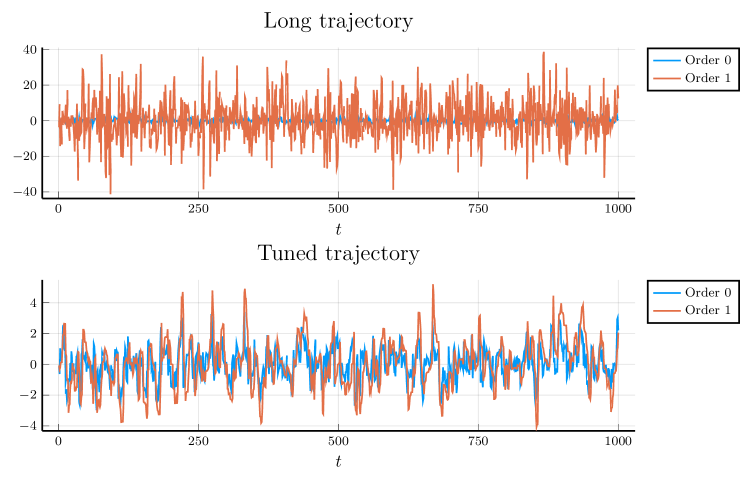
Figure 2: In the Hamiltonian approach the variance of the derivative estimators depend crucially on the trajectory length (see text for more details).

It is clear that since the HMC algorithm only integrates the eom up to a finite time $\tau$, and since we take the average over the samples, this phenomena does not represent any issue for the convergence: any trajectory length will produce correct results according with our expectations. On the other hand, it is also clear that the variance of the observables computed with these samples will depend significantly on the trajectory length: of the many solutions found by the Hamiltonian approach (corresponding to different trajectory lengths), some will produce results with smaller variances.

Figure 2 shows that for certain trajectory length, the Hamiltonian approach described here just “finds” the transformation given by Eq. (4.3): the zeroth and first order are very similar. Any other trajectory length will still produce the correct expectation values, but with a significantly larger variance. In the case of the SMD algorithm we observe a similar phenomena, but in this case it is the parameter $\gamma$ the one that has to be tuned.

This little example shows two important lessons: 1) the Hamiltonian approach can be considered just a change of variables from the original samples $x^{\alpha}\rightarrow\tilde{y}^{\alpha}(x^{\alpha})$ such that once applied to the reweighting formula eq. (3.6) gives constant reweighting factors, and 2) The variance obtained for the derivatives depends on the particular change of variables. In section 6 we will comment on the differences in variance between the two methods in detail.

5 Some general applications

In this section we explore a few applications of the techniques introduced in section 3. First we consider the application of the reweighting technique to an optimization problem. Second, we consider the application in Bayesian inference to obtain the dependence of predictions on the parameters that characterize the prior distribution.

5.1 Applications in optimization

As an example application of an optimization process we will consider the probability density function

$$p_{\theta}(x)=\frac{1}{\mathcal{Z}}\exp\left\{-S(x;\theta)\right\}\,,\qquad\left(\mathcal{Z}=\int{\rm d}x\,e^{-S(x:\theta)}\right)\,.$$ (5.1)

with

$$S(x;\theta)=\frac{1}{\theta_{1}^{2}+1}\left(x_{1}^{2}+x_{1}^{4}\right)+\frac{1}{2}x_{2}^{2}+\theta_{2}x_{1}x_{2}\,.$$ (5.2)

The shape of $S(x;\theta)$ is inspired in the action of a quantum field theory in zero dimensions, where $x_{1}$ and $x_{2}$ are two fields with coupling $\theta_{2}$, while $\theta_{1}$ is related to the mass of the field $x_{1}$. Expectation values with respect to $p_{\theta}(x)$ are functions of the parameters $\theta$.

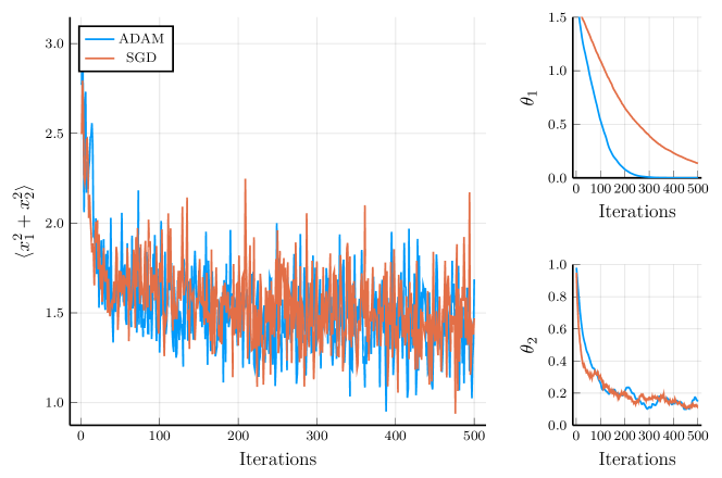
Figure 3: Estimates of the objective function $\mathbb{E}_{\theta}[x_{1}^{2}+x_{2}^{2}]$ as a function of the iteration count both for the SGD and ADAM algorithms. Both parameters $\theta_{i},\theta_{2}$ tend to their optimal value (zero).

As an example we consider the problem of minimizing $\mathbb{E}_{\theta}[x_{1}^{2}+x_{2}^{2}]$ (i.e. finding the values for $\theta$ that make $\mathbb{E}_{\theta}[x_{1}^{2}+x_{2}^{2}]$ minimum). We have implemented two flavours of Stochastic Gradient Descent (SGD): the first -basic- one, having a constant learning rate, and the second one being the well-known ADAM algorithm [14]. It is worth noting at this point that as a general concept, SGD implies a stochastic (but unbiased) evaluation of the gradients of the objective function at every iteration. While in typical applications in the ML community, where the task is to fit some dataset, this is done by evaluating the gradients at different random batches of the data, the present example is different in that no data is involved. In this case, every iteration of the SGD evaluates the gradients on the different Monte Carlo samples used to approximate the objective function $\mathbb{E}_{\theta}[x_{1}^{2}+x_{2}^{2}]$.

Here we consider a simple implementation of the Metropolis Hastings algorithm in order to first produce the samples $\{x^{\alpha}\}_{\alpha=1}^{N}\sim p_{\theta}(x)$. Second, we determine the reweighted expectation value truncated at first order

$$\frac{\sum w(x^{\alpha};\tilde{\theta})\left[(x^{\alpha}_{1})^{2}+(x_{2}^{\alpha})^{2}\right]}{\sum w(x^{\alpha};\tilde{\theta})}\approx\bar{O}+\bar{O}_{i}\epsilon_{i}\,,\qquad\left(w(x^{\alpha};\theta)=e^{S(x^{\alpha};\theta)-S(x^{\alpha};\tilde{\theta})}\right)\,,$$ (5.3)

where $\tilde{\theta}_{i}=\theta_{i}+\epsilon_{i}$. This quantity gives an stochastic estimate of the function value

$$\bar{O}=\frac{1}{N}\sum_{i=1}^{N}[x_{1}^{\alpha}]^{2}+[x_{2}^{\alpha}]^{2}\,,$$ (5.4)

and its derivatives

$$\bar{O}_{i}\approx\frac{\partial\mathbb{E}_{\theta}[x_{1}^{2}+x_{2}^{2}]}{\partial\theta_{i}}\,.$$ (5.5)

Figure 3 shows the result of the optimization process. As the iteration count increases the function is driven to its minima, while the values of the parameters approach the optimal values $\theta_{1}^{\rm opt}=\theta_{2}^{\rm opt}=0$.

It is worth mentioning that in this particular example only $1000$ samples were used at each step to estimate the loss function and its derivatives. If one decides to use a larger number of samples (say $10^{5}$), the value of the parameter $\theta_{2}$ is determined with a much better precision. Note that the direction associated with $\theta_{2}$ is much flatter, and therefore its value affects much less value of the loss function.

5.2 An application in Bayesian inference

The purpose of statistical inference is to determine properties of the underlying statistical distribution of a dataset $D=\{x_{i},y_{i}\}_{i=1}^{N}$. In many cases, the independent variables $x_{i}$ are fixed, and all the stochasticity is captured by the dependent variables $y_{i}$. As such, the data is assumed to be sampled from a certain model, specified by the likelihood, $p(y|x,\phi)$, which depends on a set of parameters $\phi$. The Bayesian paradigm attributes a level of confidence to the model by introducing the prior $p_{\theta}(\phi)$, i.e. an a priori distribution of the models parameters, where in this context $\theta$ play the role of the hyper-parameters specifying the prior. Following Bayes’ rule, the posterior distribution $p_{\theta}(\phi|D)$ is computed as:

$$p_{\theta}(\phi|D)\propto p(D|\phi)p_{\theta}(\phi)~{}.$$ (5.6)

The likelihood of the whole dataset, $p(D|\phi)$, is computed assuming independent data points following a Gaussian distribution:

$$p(D|\phi)=\prod_{i=1}^{N}\mathcal{N}(y_{i}|f(x_{i};\phi),\sigma_{i})\,,$$ (5.7)

where $\sigma_{i}$ are the uncertainties of the corresponding observations $y_{i}$ (and assumed here to be given), while the mean of the Gaussian is given by $f(x_{i};\phi)$. From a practical standpoint, in addition to the normalization being, in general, unknown, the usual complexity of the posterior distribution makes this possibly highly dimensional integral difficult to compute. The use of Monte Carlo techniques, in particular of the HMC, is typical in this context. We focus below on two types of predictions: 1) The variance of the model parameters $\delta\phi_{j}^{2}=\mathbb{E}_{p_{\theta}}[\phi_{j}^{2}]-(\mathbb{E}_{p_{\theta}}[\phi_{j}])^{2}$, where $j=1,...,d$, being $d$ the dimension of $\phi$, and 2) the variance of the output mean $\delta f_{t}^{2}=\mathbb{E}_{p_{\theta}}[f_{t}^{2}]-(\mathbb{E}_{p_{\theta}}[f_{t}])^{2}$, where $f_{t}$ is a shorthand notation for the output mean $f(x_{t};\phi)$, evaluated at a new “test” datapoint $x_{t}$ .

We are interested in studying the dependence of these quantities on the choice of hyperparameters $\theta$ that characterize the prior distributions. In particular we will consider the case of Gaussian priors, and determine the dependence of our predictions with the width of this Gaussian.

5.2.1 Model and data set

We generate a synthetic dataset (cf. Figure 4) by defining the points on an irregular grid in the range $x_{i}\in[-1.0;1.0]$, such that

$$y_{i}=f(x_{i};\phi_{\rm true})+\sigma_{i}\epsilon~{},$$ (5.8)

where the mean is a 3rd degree polynomial, $f(x;\phi)=\phi_{0}+\phi_{1}x+\phi_{2}x^{2}+\phi_{3}x^{3}$, with $\phi_{\rm true}=(1,1,1,1)$; $\epsilon\sim{\cal N}(0,1)$ is sampled from a standard Gaussian, and we consider a heteroscedastic dataset by defining a noise $\sigma_{i}$ dependent on $x_{i}$. We adopt the same model in order to make inference on the parameters $\phi$.

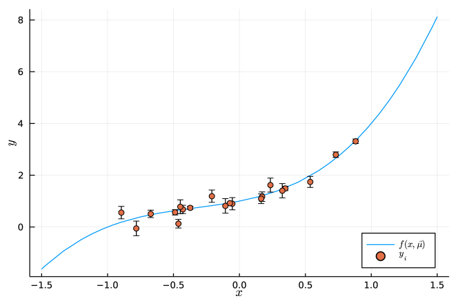
Figure 4: Third order polynomial $y(x)=1+x+x^{2}+x^{3}$ and the randomly sampled dataset $D$.

The prior distribution is also chosen as a Gaussian, $\phi\sim{\cal N}(\mu_{p},\sigma_{p})$. For simplicity we choose the priors centered on the “correct” values of the model (i.e. $\mu_{p}=\phi_{\rm true}$), while we keep the width $\sigma_{p}$ as a hyperparameter to study the dependence on.

For any choice of the prior width $\sigma_{p}$ we can obtain a prediction by generating $N$ samples $\{\phi^{(\alpha)}\}^{N}_{\alpha=1}$ according to the distribution $p_{\theta}(\phi|D)$ computed from eq. 5.6.

5.2.2 Reweighting approach

The reweighting method takes $N$ samples $\{\phi_{i}^{({\alpha})}\}_{\alpha=1}^{N}$ obtained at $\sigma_{p}=\sigma_{p}^{*}$ and computes the reweighted average using $\tilde{\sigma}_{p}=\sigma_{p}^{*}+\epsilon$ in eq. 3.3.

For each sample $\phi^{(\alpha)}$, the reweighting factor becomes a polynomial expansion in $(\sigma-\sigma_{p}^{*})$

$$\tilde{w}_{\alpha}(\epsilon)=\frac{p_{\mu,\sigma_{p}^{*}+\epsilon}(\phi_{\alpha}|D)}{p_{\mu,\sigma_{p}^{*}}(\phi_{\alpha}|D)}.$$ (5.9)

Notice that the zeroth order of eq. 5.9 is one, such that the zeroth order result corresponds to the usual Monte Carlo point estimate for $\delta\phi_{0}(\sigma_{p}^{*})$.

In order to generate these samples, we used the standard HMC algorithm. The equations of motion are

$$H_{\theta}(\phi,\pi)=\frac{\pi^{2}}{2}-\log(p_{\theta}(\phi|D)),$$ (5.10)

$$\dot{\phi}_{j}=\pi_{j},$$ (5.11)

$$\dot{\pi}_{j}=-\frac{1}{\sigma_{p}^{2}}(\phi_{j}-(\mu_{p})_{j})+\sum_{i=0}^{N}\frac{1}{\sigma_{i}^{2}}\left(y_{i}-f(x_{i},\phi)\right)(x_{i})^{j},$$ (5.12)

where $\pi=\{\pi_{0},\pi_{1},\pi_{2},\pi_{3}\}$ are the momenta conjugated to $\phi$. Note that all $\phi$-independent terms can be dropped from the equations of motion, namely the normalization of $p_{\theta}(\phi|D)$ is not needed. The eom were solved numerically using a fourth-order symplectic integrator [9] providing a high acceptance rate in the Metropolis-Hastings step even with a coarse integration.

The chosen integration step-size was $\varepsilon=0.001$, while the trajectory length was uniformly sampled in the interval $[0,100]\times\varepsilon$.

5.2.3 Hamiltonian perturbative expansion

Following the procedure in section 3.2, the Monte Carlo samples $\{(\tilde{\phi}_{j})^{\alpha}\}_{\alpha=1}^{N},~{}j=0,1,2,3$ were obtained with the modified HMC algorithm for some values of $\sigma_{p}^{*}$. We used the same parameters for the HMC as described in the previous section. In particular our acceptances were so close to 100% that any bias due to the missing accept/reject step is negligible. We checked this hypothesis by further performing another simulation with a coarser value of the integration step and finding completely compatible results.

5.2.4 Results

Table 1: Results for the expansion coefficients of the variance, ${\delta\phi^{2}_{j,n}}$ for $\sigma_{p}^{*}=0.3$ from the reweighting and hamiltonian expansion.

		$n$
		0	1	2	3	4	5
$\delta\phi^{2}_{0,n}$	RW	0.00014705(86)	0.0001384(63)	-0.000248(29)	0.000367(62)	-0.00071(51)	-0.0003(12)
	HAD	0.00014705(86)	0.0001365(34)	-0.0002850(60)	0.000311(20)	0.000178(77)	-0.00115(26)
$\delta\phi^{2}_{1,n}$	RW	0.01099(15)	0.0285(12)	-0.0450(58)	0.032(13)	0.04(10)	-0.61(25)
	HAD	0.01099(15)	0.02787(69)	-0.0518(11)	0.0248(38)	0.189(16)	-0.700(46)
$\delta\phi^{2}_{2,n}$	RW	0.008938(74)	0.00830(28)	-0.0283(10)	0.0850(39)	-0.234(18)	0.603(78)
	HAD	0.008938(74)	0.00817(15)	-0.02789(42)	0.0849(13)	-0.2505(44)	0.726(15)
$\delta\phi^{2}_{3,n}$	RW	0.03617(59)	0.1205(51)	-0.182(24)	0.050(61)	0.63(42)	-4.0(12)
	HAD	0.03617(59)	0.1177(30)	-0.2052(42)	0.020(16)	1.132(66)	-4.02(19)

Here we compare the predictions for the average model parameters $\phi$ and their dependence on the prior width $\sigma$. In particular we focus on the variance of the model parameters $\delta\phi^{2}_{j}$, since these are the quantities most sentitive to the prior width (i.e. very thin priors result in small variance for the model parameters). We have fixed $\sigma^{*}=0.3$, but similar conclusions are obtained for other values.

The results of the Monte Carlo average for $\delta\tilde{\phi}^{2}_{i}$ and its derivatives with respect to $\sigma$ are shown in LABEL:tab:variance_phi0. Results labeled “RW” use the reweighting method, while results labeled “HAD” use the Hamiltonian approach.

It is obvious that results using the Hamiltonian approach are more precise: the uncertainties in the derivatives, $\delta\phi^{2}_{i,n},n\neq 0$, are smaller for the Hamiltonian approach, despite the statistics being the same. The difference is larger for higher order derivatives: the approach based on reweighting struggles to get a signal for the fourth and fifth derivatives, while the Hamiltonian approach is able to obtain even the fifth derivative with a few percent precision. This fits our expectations (see section 4).

On the other hand, for our second quantity of analysis $\delta f_{t}^{2}$ (i.e. the variance of the prediction mean), Figure 5 shows the results of the dependence on $\sigma_{p}$, where we have fixed $x_{t}=0.5$.

The Hamiltonian approach gives visually results with a reduced variance, similar to the results presented in table LABEL:tab:variance_phi0.

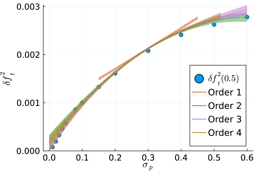
(a) Reweighting approach

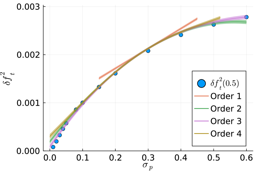
(b) Hamiltonian approach

Figure 5: Variance of the prediction $\mathbb{E}_{p_{\theta}}[f(x_{t},\phi)]$ for a new point $x_{t}=0.5$ as a function of $\sigma_{p}$. The blue points represent simulations at different values of $\sigma_{p}$. The error bands represent the evaluation of the Taylor series (up to $\order{(\sigma-\sigma_{p}^{*})^{4}}$ with $\sigma_{p}^{*}=0.3$) where derivatives are obtained with the Hamiltonian based approach (right) or the reweighting approach (left). The Hamiltonian approach gives more precise results.

6 A case study in lattice field theory

In this section we explore in detail some applications in lattice field theory. We will use as model the $\lambda-\phi^{4}$ theory in 4 space-time dimensions. In the continuum the Euclidean action of this theory is given by

$$S(\phi;m,\lambda)=\int{\rm d}x^{4}\left\{\frac{1}{2}(\partial_{\mu}\phi)^{2}+\frac{m^{2}}{2}\phi^{2}+\lambda\phi^{4}\right\}\,.$$ (6.1)

The discretized version of this action is

$$S_{\rm latt}(\hat{\phi};\hat{m},\lambda)=\sum_{x}\left\{\frac{1}{2}\sum_{\mu}[\hat{\phi}(x+\hat{\mu})-\hat{\phi}(x)]^{2}+\frac{\hat{m}^{2}}{2}\hat{\phi}^{2}(x)+\lambda\hat{\phi}^{4}(x)\right\}$$ (6.2)

where dimension-full quantities have been scaled with appropriate powers of the lattice spacing $a$ in order to render all quantities dimensionless

$$\hat{\phi} = a\phi\,,$$ (6.3)

$$\hat{m} = am\,.$$ (6.4)

In field theory one is interested in correlation functions, given as expectation values over the Euclidean partition function

$$\mathcal{Z}=\int\prod_{x}{\rm d}\hat{\phi}(x)e^{-S_{\rm latt}(\hat{\phi};\hat{m},\lambda)}\,.$$ (6.5)

These expectation values depend on the parameters $\hat{m},\lambda$. The methods described in sections 3.1 and 3.2 can be applied to determine the dependence of correlation functions with these parameters. In particular we note that for non-negative $\hat{m}^{2}$ the potential given by the action of eq. (6.2) is convex, guaranteeing the convergence of the Hamiltonian perturbative expansion (see section 3.2.1).

We have performed simulations on a $L^{4}$ lattice with $L/a=32,48$ for several values of the parameter $\lambda$ and $\hat{m}^{2}=0.05$. As example observables, we will consider some simple local quantities: $\langle\hat{\phi}^{2}(x)\rangle,\langle\hat{\phi}^{4}(x)\rangle$, as well as the action density

$$\langle\hat{s}(x)\rangle=\frac{1}{2}\langle[\hat{\phi}(x+\hat{\mu})-\hat{\phi}(x)]^{2}\rangle+\frac{\hat{m}^{2}}{2}\langle\hat{\phi}^{2}(x)\rangle+\lambda\langle\hat{\phi}^{4}(x)\rangle\,.$$ (6.6)

Since we perform our simulations with periodic boundary conditions, invariance under translations ensures that these local expectation values are independent on the point measured $x$. In order to get better precision we perform volume averages for the estimations (e.g. $\langle\tilde{s}\rangle=\left(\frac{a}{L}\right)^{4}\sum_{x}\langle\tilde{s}(x)\rangle$).

Table 2 shows the results of both the Hamiltonian and the reweighting approach applied to the determination of the derivatives $\partial/\partial m^{2}$, $\partial/\partial\lambda$, $\partial^{2}/\partial m^{2}\partial\lambda$ of the observables $\langle\phi^{2}\rangle,\langle\phi^{4}\rangle,\langle\hat{s}\rangle$ (see eq. (6.6)).

			$\lambda$
			0.0	0.1	0.2	0.3	0.4	0.5
$\langle\phi^{2}\rangle$	$\partial_{\hat{m}^{2}}$	RW	-0.0428(20)	-0.0328(14)	-0.0270(13)	-0.0241(12)	-0.0220(11)	-0.01974(91)
		HAD	-0.042526(41)	-0.030880(14)	-0.026273(10)	-0.0233672(82)	-0.0212721(72)	-0.0196387(60)
	$\partial_{\lambda}$	RW	-0.0779(22)	-0.05227(94)	-0.04370(89)	-0.03534(61)	-0.03169(50)	-0.02754(49)
		HAD	-0.077816(79)	-0.052499(24)	-0.042218(19)	-0.035830(14)	-0.031323(11)	-0.0278909(93)
	$\partial^{2}_{\hat{m}^{2},\lambda}$	RW	0.43(43)	0.03(16)	0.16(14)	-0.10(11)	0.116(77)	-0.024(69)
		HAD	0.2733(22)	0.061593(99)	0.035082(69)	0.024240(42)	0.018263(31)	0.014553(31)
$\langle\phi^{4}\rangle$	$\partial_{\hat{m}^{2}}$	RW	-0.0391(20)	-0.0272(12)	-0.0223(11)	-0.01809(90)	-0.01645(86)	-0.01398(70)
		HAD	-0.038919(39)	-0.026247(13)	-0.0211084(97)	-0.0179118(73)	-0.0156615(62)	-0.0139464(46)
	$\partial_{\lambda}$	RW	-0.0844(24)	-0.0539(11)	-0.04281(92)	-0.03340(54)	-0.02850(43)	-0.02428(41)
		HAD	-0.084330(78)	-0.054229(26)	-0.041514(19)	-0.033715(14)	-0.028357(11)	-0.0243679(73)
	$\partial^{2}_{\hat{m}^{2},\lambda}$	RW	0.41(44)	0.01(16)	0.11(14)	-0.083(90)	0.089(61)	-0.000(56)
		HAD	0.2848(21)	0.068858(94)	0.038917(70)	0.026391(38)	0.019393(29)	0.015080(25)
$\langle s\rangle$	$\partial_{\hat{m}^{2}}$	RW	-0.0025(42)	-0.0006(34)	0.0027(35)	0.0028(36)	0.0057(32)	0.0063(30)
		HAD	-0.000003(22)	0.002623(16)	0.004218(20)	0.005397(14)	0.006265(16)	0.006989(15)
	$\partial_{\lambda}$	RW	-0.0686(48)	-0.0567(26)	-0.0538(25)	-0.0447(23)	-0.0400(17)	-0.0343(17)
		HAD	-0.069774(49)	-0.057738(34)	-0.050128(40)	-0.044530(27)	-0.040250(27)	-0.036721(26)
	$\partial^{2}_{\hat{m}^{2},\lambda}$	RW	1.1(1.0)	-0.16(39)	0.36(43)	-0.43(32)	0.16(26)	-0.15(21)
		HAD	0.038864(96)	0.019197(66)	0.013405(69)	0.010126(50)	0.007860(47)	0.006407(48)

Table 2: Derivatives with respect to $\hat{m}^{2}$ ($\partial_{\hat{m}^{2}}$), $\lambda$ ($\partial_{\lambda}$) and the cross derivative ($\partial^{2}_{\hat{m}^{2},\lambda}$) of different observables. Note that the action density $s$ has an explicit dependence on $\hat{m}^{2},\lambda$ (see Eq. (6.6)). All simulations are performed on a $L^{4}$ lattice with $L/a=32$ and $\hat{m}^{2}=0.05$.

It is apparent that results obtained with the Hamiltonian approach are much more precise (both results use exactly the same statistics), usually about 100 times more precise for the first derivatives. This difference in precision is even more clear for the higher orders: the signal for the cross derivative $\partial^{2}_{\hat{m}^{2},\lambda}$ is completely lost in the reweighting approach, whereas the Hamiltonian approach determines its value with a precision better than a 1%. This can be understood from a general point of view by noting that the reweighting approach requires to evaluate the so called disconnected contributions. For example, the leading order derivative $\partial_{\hat{m}^{2}}\langle\phi^{2}\rangle$ as determined by the reweighting approach is given by

$$\partial_{\hat{m}^{2}}\langle\hat{\phi}^{2}\rangle=\langle\hat{\phi}^{2}(\partial_{\hat{m}^{2}}S_{\rm latt})\rangle-\langle\hat{\phi}^{2}\rangle\langle\partial_{\hat{m}^{2}}S_{\rm latt}\rangle$$ (6.7)

These disconnected contributions are known to suffer from a large variance. As explained in section 4 the Hamiltonian approach completely avoids estimating such disconnected contributions. The Hamiltonian approach implements an exact version of the reparametrization trick, where the field variables $\tilde{\phi}(x)$ (and its dependence with the relevant parameters) are determined to any order so that all terms in the Taylor series are determined as connected contributions.

We conclude that it is the absence of disconnected terms in the Hamiltonian approach what lies at the heart of the differences in variances between both approaches.

7 Conclusions

The tools of automatic differentiation represent a cornerstone in modern optimization algorithms and many machine learning applications. The extension of these techniques to functions evaluated using Monte Carlo processes is non trivial. In these cases the underlying probability distribution depends on some parameters, and Monte Carlo techniques are used to draw samples for specific values of the parameters. The dependence of the samples with the parameter values is difficult to determine. Nonetheless, there are many applications for these techniques. In this work we have considered several of them, from optimizations of expectation values, to the study of the dependence of Bayesian predictions with respect to prior parameters or applications in lattice field theory.

We have presented two different approaches to the determination of Taylor series of quantities estimated via Monte Carlo sampling. The first approach is based on reweighting and can be considered a generalization of the score function estimator, valid for derivatives of arbitrary orders, and unnormalized probability distribution functions. The second approach is based on Hamiltonian methods to sampling (HMC being the most popular option), and produces samples that carry the information of the dependence on the action parameters. The convergence of the stochastic process in this last approach is not always guaranteed, but we have provided sufficient conditions for the convergence.

We have shown some applications of these methods. First, in the context of optimization, we have applied the stochastic gradient descent to find the optimal parameters of some expectation value (see section 5.1). Second, in Bayesian inference we have shown how these methods can be used to estimate the dependence on Bayesian predictions on the “hyperparameters” that describe the prior distribution (cf section 5.2).

Finally, in the context of Lattice Field Theory, we have studied in detail the case of $\lambda-\phi^{4}$ in four space-time dimensions. The dependence of observables with respect to the parameters of the action (the bare mass in lattice units $\hat{m}$ and the bare coupling $\lambda$) can be accurately determined using these techniques.

A detailed comparison of both methods shows that results obtained with the Hamiltonian approach are much more precise. We have argued that the Hamiltonian approach can be seen as a change of variables from the reweighing formula where the reweighing factors are constant: In the Hamiltonian approach all dependence with respect to the parameters is present in the samples. The absence of disconnected contributions (in the lattice jargon) makes the variance of Taylor series computed with the Hamiltonian approach much more precise. For example, our study on $\lambda-\phi^{4}$ shows that for the same statistics one gets results 100 times more precise.

The Hamiltonian approach has his own drawbacks. On one hand the convergence of the stochastic process is not guaranteed. In particular for the case of Lattice QCD, that is formulated in terms of compact variables, the convergence cannot be guaranteed. On the other hand, the method cannot be applied to samples that have already been generated, unlike the reweighting method.

Nevertheless the investigations of this work open the door to an interesting possibility: that one can find change of variables that eliminate (or significantly reduce) the disconnected contributions of the reweighing approach. Machine Learning techniques, in particular the tools related with normalizing flows, potentially can provide a significant gain in the computation of derivatives of expectation values.

References

- [1] G. Jerfel, S. Wang, C. Fannjiang, K. A. Heller, Y. Ma, and M. I. Jordan, “Variational refinement for importance sampling using the forward kullback-leibler divergence,” 2021. https://arxiv.org/abs/2106.15980.
- [2] M. Figurnov, S. Mohamed, and A. Mnih, “Implicit reparameterization gradients,” CoRR abs/1805.08498 (2018) , 1805.08498. http://arxiv.org/abs/1805.08498.
- [3] V. Liévin, A. Dittadi, A. Christensen, and O. Winther, “Optimal variance control of the score function gradient estimator for importance weighted bounds,”. https://arxiv.org/abs/2008.01998.
- [4] Y. Cong, M. Zhao, K. Bai, and L. Carin, “GO gradient for expectation-based objectives,” in International Conference on Learning Representations. 2019. https://openreview.net/forum?id=ryf6Fs09YX.
- [5] A. Haro, “Automatic differentiation methods in computational dynamical systems: Invariant manifolds and normal forms of vector fields at fixed points,”.
- [6] S. Duane, A. Kennedy, B. J. Pendleton, and D. Roweth, “Hybrid monte carlo,” Physics Letters B 195 no. 2, (1987) 216–222.
- [7] N. Bou-Rabee and J. M. Sanz-Serna, “Randomized hamiltonian monte carlo,” The Annals of Applied Probability 27 no. 4, (Aug, 2017) . http://dx.doi.org/10.1214/16-AAP1255.
- [8] M. Luscher and S. Schaefer, “Non-renormalizability of the HMC algorithm,” JHEP 04 (2011) 104, arXiv:1103.1810 [hep-lat].
- [9] I. Omelyan, I. Mryglod, and R. Folk, “Symplectic analytically integrable decomposition algorithms: classification, derivation, and application to molecular dynamics, quantum and celestial mechanics simulations,” Computer Physics Communications 151 no. 3, (2003) 272–314.
- [10] M. D. Brida and M. Lüscher, “SMD-based numerical stochastic perturbation theory,” Eur. Phys. J. C 77 no. 5, (May, 2017) 308. http://arxiv.org/abs/1703.04396. arXiv:1703.04396 [hep-lat].
- [11] F. Di Renzo, G. Marchesini, P. Marenzoni, and E. Onofri, “Lattice perturbation theory on the computer,” Nucl. Phys. B Proc. Suppl. 34 (1994) 795–798.
- [12] M. Dalla Brida, M. Garofalo, and A. D. Kennedy, “Investigation of new methods for numerical stochastic perturbation theory in theory,” Phys. Rev. D 96 (Sep, 2017) 054502.
- [13] M. D. Brida, M. Garofalo, and A. D. Kennedy, “Numerical stochastic perturbation theory and gradient flow in theory,” 2015.
- [14] D. P. Kingma and J. Ba, “Adam: A method for stochastic optimization,” 2017.