Fermion states localized
on a self-gravitating non-Abelian monopole

Abstract

We study fermionic modes localized on the static spherically symmetric self-gravitating non-Abelian monopole in the $SU(2)$ Einstein-Dirac-Yang-Mills-Higgs theory. We consider dependence of the spectral flow on the effective gravitational coupling constant and show that, in the limiting case of transition to the Reissner-Nordström black hole, the fermion modes are fully absorbed into the interior of the black hole.

I Introduction

Various black holes with localized matter fields, which circumvent the no-hair theorem (see, e.g., [1, 2, 3] and references therein), are rather a common presence in the landscape of gravity solutions. The most well-known examples in (3+1)-dimensional asymptotically flat spacetime are static hairy black holes with spherically symmetric event horizon in the $SU(2)$ Einstein-Yang-Mills theory [4, 5, 6], black holes with Skyrmion hairs [7, 8, 9] and black holes inside magnetic monopoles [10, 11, 12]. Various generalizations of solutions of that type with different types of hairs were considered over last decade. In particular, there are spinning black holes with scalar hairs both in the Einstein-Klein-Gordon theory [14, 15] and in the non-linear O(3) sigma model [16], dyonic black holes in Einstein-Yang-Mills-Higgs theory [17, 18] and black holes with axionic hairs [19, 20]. There are also hairy black holes supporting the stationary Proca hair [21] and electrostatic charged black holes [22, 23, 24].

In most cases, such solutions can be viewed as a small black hole immersed inside a localized field configuration, the horizon radius $r_{h}$ cannot be arbitrary large. The limiting case of the event horizon shrinking to zero corresponds to the regular self-gravitating lump, which may also possess a flat space solitonic limit. The corresponding solutions may represent a topological soliton, like monopoles [25, 26] and Skyrmions [27, 28], or a non-topological solitons, like Q-balls [29, 30, 31]. There is also another class of spinning hairy black holes which do not possess the solitonic limit, like black holes with stationary Klein-Gordon hair [14, 15] or black holes with Yang-Mills hair [4, 5, 6].

On the other hand, some of hairy black holes with finite horizon radius may bifurcate with the vacuum black holes, as it happens, for example, with the black holes with monopole hair, they smoothly approach the extremal Reissner-Nordström solution [10, 11, 12, 13]. Another scenario is that there is a mass gap between hairy black holes and corresponding vacuum solutions with an event horizon. This situation takes place for black holes with Skyrmion hairs [7, 8, 9] and for the black holes with pure Yang-Mills hairs on the Schwarzschild background [4, 5, 6].

A notable exception in the variety of asymptotically flat solutions of General Relativity in (3+1) dimensions, which circumvents the no-hair theorems, is a missing class of black holes with fermionic hairs. Although there are regular localized solutions of the Einstein-Dirac and Einstein-Maxwell-Dirac equations [32, 33, 34, 35, 36, 37, 38], all attempts to extend these solutions to the case of finite event horizon has been failed: the spinor modes, which are gravitationally bound in the black hole spacetime decay due to the absence of superradiance mechanism for the Dirac field [39]. On the other hand, black holes with fermionic hairs are known to exist in the gauged $d=4,5$ $N=2$ supergravity [40, 41]; here the $N=2$ extremal black holes represent $1/2$ Bogomolnyi-Prasad-Sommerfield (BPS) states [42] with a set of fermion zero modes. Appearance of these modes is related with remarkable relation between the topological charge of the field configuration and the number of zero modes, exponentially localized on a soliton: the fundamental Atiyah-Patodi-Singer index theorem [43] requires one normalizable fermion zero mode per unit topological charge. Recently, massless electroweak fermions in the near horizon region of black hole we discussed in Ref. [44].

The fermion modes localized on a soliton are well known and are exemplified by the spinor modes of the kinks [45, 46], vortices [47, 48], Skyrmions [49, 50] and monopoles [46, 51, 52]. In supersymmetric theories the fermion zero modes are generated via supersymmetry transformations of the boson field of the static soliton; breaking of supersymmetry yields a spectral flow of the eigenvalues of the Dirac operator with some number of normalizable bounded modes crossing zero. However, little is known about evolution of the bounded fermionic modes in the presence of gravity, especially as the self-gravitating soliton approaches the critical limit and bifurcates with a black hole.

In this Letter we investigate numerically a self-gravitating non-Abelian monopole-fermion system with back-reaction and elucidate the mechanism for disappearance of the fermionic modes. Our computations reveal that as the BPS monopole bifurcates with the extremal Reissner-Nordström solution, the fermionic modes become absorbed into the interior of the black hole. Further, we show that this observation also holds for non-BPS monopoles with localized non-zero modes.

II The Model

We consider the (3+1)-dimensional $SU(2)$ Einstein-Yang-Mills-Higgs system, coupled to a spin-isospin field $\psi_{\alpha i}$. The model has the following action (we use natural units with $c=\hbar=1$ throughout):

$$S=\int d^{4}x~{}\sqrt{-g}\left[-\frac{R}{16\pi G}-\frac{1}{2}{\rm Tr}(F_{\mu\nu}F^{\mu\nu})+{\rm Tr}(D_{\mu}\phi~{}D^{\mu}\phi)-\frac{\lambda}{4}{\rm Tr}\left(\phi^{2}-\phi_{0}^{2}\right)^{2}+L_{\text{sp}}\,\right],$$ (1)

where $R$ is the scalar curvature, $G$ is Newton’s gravitational constant, $g$ denotes the determinant of the metric tensor, and the field strength tensor of the gauge field $A_{\mu}=\frac{1}{2}A_{\mu}^{a}\tau^{a}$ is

$$F_{\mu\nu}=\partial_{\mu}A_{\nu}-\partial_{\nu}A_{\mu}+ie[A_{\mu},A_{\nu}]\,,$$

where $a=1,2,3$ is a color index, $\mu,\nu=0,1,2,3$ are spacetime indices, and $\tau^{a}$ are the Pauli matrices. The covariant derivative of the scalar field in adjoint representation $\phi=\phi^{a}\tau^{a}$ is

$$D_{\mu}\phi=\partial_{\mu}\phi+ie[A_{\mu},\phi],$$

where $e$ is the gauge coupling constant. The scalar potential with a Higgs vacuum expectation value $\phi_{0}$ breaks the $SU(2)$ symmetry down to $U(1)$ and the scalar self-interaction constant $\lambda$ defines the mass of the Higgs field, $M_{s}=\sqrt{\lambda}\phi_{0}$. The gauge field becomes massive due to the coupling with the scalar field, $M_{v}=e\phi_{0}$.

Bosonic sector of the model $(\ref{lgr_10})$ is coupled to the Dirac isospinor fermions $\psi_{\alpha i}$ with the Lagrangian [46]

$$L_{\text{sp}}=\frac{\imath}{2}\left((\hat{\not{D}}\bar{\psi})\psi-\bar{\psi}\hat{\not{D}}\psi\right)-m\bar{\psi}\psi-\frac{\imath}{2}h\bar{\psi}\gamma^{5}\phi\psi\,,$$ (2)

where $m$ is a bare mass of the fermions, $h$ is the Yukawa coupling constant, $\gamma^{\mu}$ are the Dirac matrices in the standard representation in a curved spacetime, $\gamma^{5}$ is the corresponding Dirac matrix defined in Appendix A, $\hat{\not{D}}=\gamma^{\mu}\hat{D}_{\mu}$ and the isospinor covariant derivative on a curved spacetime is defined as (see, e.g., Ref. [39])

$$\hat{D}_{\mu}\psi=(\partial_{\mu}-\Gamma_{\mu}+ieA_{\mu})\psi.$$

Here $\Gamma_{\mu}$ are the spin connection matrices [39]. Explicitly, in component notations, we can write

$$\hat{D}_{\mu}\psi_{\alpha i}\equiv\left[\delta_{ij}(\partial_{\mu}-\Gamma_{\mu})-\frac{\imath e}{2}(\tau^{a})_{ij}A^{a}_{\mu}\right]\psi_{\alpha i}$$

with the group indices $i,j$ taking the values $1,2$ and the Lorentz index $\alpha$ takes the values $0\dots 3$.

Variation of the action (1) with respect to the metric leads to the Einstein equations

$$R_{\mu\nu}-\frac{1}{2}g_{\mu\nu}R=8\pi G\left[\left(T_{\mu\nu}\right)_{YM}+\left(T_{\mu\nu}\right)_{\phi}+\left(T_{\mu\nu}\right)_{s}\right]$$ (3)

with the pieces of the total stress-energy tensor

$$\begin{split}\left(T_{\mu\nu}\right)_{YM}=&-F^{a}_{\mu\alpha}F^{a}_{\nu\beta}g^{\alpha\beta}+\frac{1}{4}g_{\mu\nu}F^{2}\,,\\ \left(T_{\mu\nu}\right)_{\phi}=&D_{\mu}\phi^{a}D_{\nu}\phi^{a}-g_{\mu\nu}\left[\frac{1}{2}D_{\alpha}\phi^{a}D^{\alpha}\phi^{a}-\frac{\lambda}{4}\left(\phi^{2}-\phi_{0}^{2}\right)^{2}\right]\,,\\ \left(T_{\mu\nu}\right)_{s}=&\frac{\imath}{4}\left[\bar{\psi}\gamma_{\mu}(\hat{D}_{\nu}\psi)+\bar{\psi}\gamma_{\nu}(\hat{D}_{\mu}\psi)-(\hat{D}_{\mu}\bar{\psi})\gamma_{\nu}\psi-(\hat{D}_{\nu}\bar{\psi})\gamma_{\mu}\psi\right]-g_{\mu\nu}L_{\text{sp}}\,.\end{split}$$ (4)

The corresponding matter field equations are:

$$\begin{split}D_{\nu}F^{a\nu\mu}&=-e\epsilon^{abc}\phi^{b}D^{\mu}\phi^{c}-\frac{e}{2}\bar{\psi}\gamma^{\mu}\sigma^{a}\psi\,,\\ D_{\mu}D^{\mu}\phi^{a}&+\lambda\phi^{a}\left(\phi^{2}-\phi_{0}^{2}\right)+\imath h\bar{\psi}\gamma^{5}\sigma^{a}\psi=0\,,\\ \imath\hat{\not{D}}\psi&-\imath\frac{h}{2}\gamma^{5}\sigma^{a}\phi^{a}\psi-m\psi=0.\end{split}$$ (5)

III Equations and solutions

Working within the above model, in this section we present general spherically symmetric equations and solve them numerically for some values of system parameters.

III.1 The Ansatz

For the gauge and Higgs field we employ the usual static spherically symmetric hedgehog Ansatz [25, 26]

$$A_{0}^{a}=0,\quad A_{i}^{a}=\varepsilon_{aik}\frac{r^{k}}{er^{2}}\left[1-W(r)\right],\qquad\phi^{a}=\frac{r^{a}}{er}H(r)\,.$$ (6)

The spherically symmetric Ansatz with a harmonic time dependence for the isospinor fermion field localized by the monopole can be written in terms of two $2\times 2$ matrices $\chi$ and $\eta$ [46, 53] as

$$\psi=e^{-\imath\omega t}\begin{pmatrix}\chi\\ \eta\end{pmatrix}\quad\text{with}\quad\chi=\frac{u(r)}{\sqrt{2}}\begin{pmatrix}0&-1\\ 1&0\end{pmatrix},\eta=\imath\frac{v(r)}{\sqrt{2}}\begin{pmatrix}\sin\theta e^{-\imath\varphi}&-\cos\theta\\ -\cos\theta&-\sin\theta e^{\imath\varphi}\end{pmatrix}.$$

Here $u(r)$ and $v(r)$ are two real functions of the radial coordinate only and $\omega$ is the eigenvalue of the Dirac operator.

For the line element we employ Schwarzschild-like coordinates, following closely the usual consideration of gravitating monopole (see, e.g., Refs. [11, 12])

$$ds^{2}=\sigma(r)^{2}N(r)dt^{2}-\frac{dr^{2}}{N(r)}-r^{2}(d\theta^{2}+\sin^{2}\theta d\varphi^{2}).$$ (7)

The metric function $N(r)$ can be rewritten as $N(r)=1-\frac{2G\mu(r)}{r}$ with the mass function $\mu(r)$; the ADM mass of the configuration is defined as $M=\mu(\infty)$. The above metric implies the following form of the orthonormal tetrad:

$$e^{a}_{\phantom{a}\mu}=\text{diag}\left\{\sigma\sqrt{N},\frac{1}{\sqrt{N}},r,r\sin\theta\right\},$$

such that $ds^{2}=\eta_{ab}(e^{a}_{\mu}dx^{\mu})(e^{b}_{\nu}dx^{\nu})$, where the Minkowski metric $\eta_{ab}=(+1,-1,-1,-1)$ and $\gamma^{\mu}=e^{\mu}_{\phantom{a}a}\hat{\gamma}^{a}$ with $\hat{\gamma}^{a}$ being the usual flat space Dirac matrices.

III.2 Equations

Substitution of the Ansatz (6)-(7) into the general system of equations (3) and (5) yields the following set of six coupled ordinary differential equations for the functions $W,H,u,v,N,\sigma$ (here the prime denotes differentiation with respect to the radial coordinate, $\sigma^{\prime}=\frac{d\sigma}{dr}$, etc. ):

$$\frac{\sigma^{\prime}}{\sigma}=\alpha^{2}\left[2\frac{W^{\prime 2}}{x}+xH^{\prime 2}-\frac{2W+hxH}{N}uv+2\omega\frac{x\left(u^{2}+v^{2}\right)}{N^{3/2}\sigma}-m\frac{x\left(u^{2}-v^{2}\right)}{N}\right]\,,$$ (8)

$$N^{\prime}+\frac{1}{x}\left(N-1\right)=-\alpha^{2}\Big{[}2\frac{NW^{\prime 2}}{x}+xNH^{\prime 2}+\frac{\left(1-W^{2}\right)^{2}}{x^{3}}+2\frac{W^{2}H^{2}}{x}+\frac{\beta^{2}}{2}x\left(1-H^{2}\right)^{2}$$

$$+2\omega\frac{x\left(u^{2}+v^{2}\right)}{\sqrt{N}\sigma}\Big{]}\,,$$ (9)

$$W^{\prime\prime}+\left(\frac{N^{\prime}}{N}+\frac{\sigma^{\prime}}{\sigma}\right)W^{\prime}+\frac{\left(1-W^{2}\right)}{Nx^{2}}W=\frac{WH^{2}}{N}+\frac{xuv}{N}\,,$$ (10)

$$H^{\prime\prime}+\left(\frac{2}{x}+\frac{N^{\prime}}{N}+\frac{\sigma^{\prime}}{\sigma}\right)H^{\prime}-2\frac{W^{2}H}{Nx^{2}}+\frac{\beta^{2}}{N}\left(1-H^{2}\right)H-2h\frac{uv}{N}=0\,,$$ (11)

$$u^{\prime}+u\left(-\frac{W}{\sqrt{N}x}-\frac{h}{2}\frac{H}{\sqrt{N}}+\frac{1}{4}\frac{N^{\prime}}{N}+\frac{1}{x}+\frac{1}{2}\frac{\sigma^{\prime}}{\sigma}\right)+v\left(\frac{\omega}{N\sigma}+\frac{m}{\sqrt{N}}\right)=0\,,$$ (12)

$$v^{\prime}+v\left(\frac{W}{\sqrt{N}x}+\frac{h}{2}\frac{H}{\sqrt{N}}+\frac{1}{4}\frac{N^{\prime}}{N}+\frac{1}{x}+\frac{1}{2}\frac{\sigma^{\prime}}{\sigma}\right)-u\left(\frac{\omega}{N\sigma}+\frac{m}{\sqrt{N}}\right)=0\,.$$ (13)

Here we define a new dimensionless radial coordinate, $x=e\phi_{0}r$, and three rescaled effective coupling constants $\alpha^{2}=4\pi G\phi_{0}^{2}\,,\beta^{2}=\frac{\lambda}{e^{2}}\,,\tilde{h}=\frac{h}{e}$. The scaled bare mass parameter and the eigenfrequency of the fermion field are $\tilde{m}=\frac{m}{e\phi_{0}}$ and $\tilde{\omega}=\frac{\omega}{g\phi_{0}}$, respectively. The fermion field scales as $\psi\to\psi/(\sqrt{e}\phi_{0}^{3/2})$. To simplify the formulas, we will drop the tilde notation henceforth. Also, in what follows, we restrict ourselves to the case of fermions with zero bare mass setting $m=0$. Hence, the solutions depend essentially on three dimensionless parameters given by the mass ratios

$$\alpha=\sqrt{4\pi}\frac{M_{v}}{eM_{Pl}},\quad\beta=\frac{M_{s}}{M_{v}},\quad h=\frac{2M_{f}}{M_{v}},$$

where $M_{Pl}=G^{-1/2}$ is the Plank mass and $M_{v}=e\phi_{0}$, $M_{s}=\sqrt{\lambda}\phi_{0}$ and $M_{f}=h\phi_{0}/2$ are the masses of the gauge field, Higgs field and fermion field, respectively.

The system of equations (8)-(13) is supplemented by the normalization condition of the localized fermion mode

$$\int dV\,\psi^{\dagger}\psi=\frac{4\pi}{e^{2}}\int_{0}^{\infty}\frac{\tilde{u}^{2}+\tilde{v}^{2}}{\sqrt{N}}x^{2}dx=1.$$ (14)

Note that, as $\omega\neq 0$, the metric field $\sigma$ cannot be eliminated from the system (8)-(13), as is done, for example, for a self-gravitating monopole (see, e.g., Ref. [1]).

The system (8)-(13) admits embedded Reissner-Nordström (RN) solution [57, 58]; for the case of unit magnetic charge it reads

$$\sigma=1\,,\quad\mu(x)=\mu_{\infty}-\frac{\alpha^{2}}{2x}\,,\quad W=0\,,\quad H=1\,,u=v=0.$$ (15)

A horizon occurs when $N(x)\to 0$, in the Schwarzschild-like parametrization it happens at some finite critical value of $x=x_{\text{cr}}=\alpha_{\text{cr}}$.

III.3 Numerical results

The system (1) possesses two limits. The flat space monopole corresponds to the case $\alpha=0$; further, setting $\beta=0$, yields the familiar self-dual BPS solution [54, 55] (see also Ref. [56] for a review),

$$W(x)=\frac{x}{\sinh x}\,,\qquad H(x)=\coth x-\frac{1}{x}.$$ (16)

There is a remarkable flat space solution for the background isospin fermion zero ($\omega=0$) mode [46, 53]. Indeed, in this case the last pair of equations (8)-(13) is decoupled, and it is reduced to

$$\begin{split}u^{\prime}+u\left(\frac{1-W}{x}-\frac{h}{2}H\right)&=0\,,\\ v^{\prime}+v\left(\frac{1+W}{x}+\frac{h}{2}H\right)&=0.\end{split}$$ (17)

Using the vacuum boundary conditions, we can see that the linearized asymptotic equations for the spinor components approaching the vacuum are

$$u^{\prime}-\frac{hu}{2}+\omega v\approx 0\,,\qquad v^{\prime}+\frac{hv}{2}-\omega u\approx 0.$$

Therefore, gravitationally localized fermion modes with exponentially decaying tail may exist if $\omega^{2}<h^{2}/4$.

The normalizable solution for the localized zero mode is

$$v=0\,,\qquad u\sim\exp\left\{-\int dx^{\prime}\,\left[\frac{1-W(x^{\prime})}{x^{\prime}}-\frac{h}{2}H(x^{\prime})\right]\right\}\,,$$

and it exists only for non-zero negative values of the scaled Yukawa coupling $h$. For example, setting $h=-2$ and making use of the exact BPS monopole solution (16), we obtain

$$v=0\,,\qquad u=\frac{1}{\cosh^{2}(x/2)}\,.$$ (18)

In our numerical calculations we used these closed form BPS solutions as a input.

Another limit $h\to 0$ while $\beta$ is kept fixed, corresponds to the decoupled fermionic sector. In such a case the well known pattern of evolution of the self-gravitating monopole is recovered, a branch of gravitating solutions emerges smoothly from the flat space monopole as the effective gravitational coupling $\alpha$ increases from zero and $\beta$ remains fixed [10, 11, 12]. Along this branch the metric function $N(x)$ develops a minimum, which decreases monotonically. The branch terminated at a critical value $\alpha_{\text{cr}}$ at which the gravitating monopole develops a degenerate horizon and configuration collapses into the extremal Reissner-Nordström black hole, as displayed in the left panel of Fig. 1. A short backward branch of unstable solutions arises in the BPS limit $\beta=0$ at $\alpha=\alpha_{\text{max}}$, it bends backwards and bifurcates with the branch of extremal RN solutions of unit magnetic charge at $\alpha_{\text{cr}}<\alpha_{\text{max}}$ [10]. Note that the ADM mass of the monopole coupled to the fermion zero mode remains the same as the mass of the pure self-gravitating monopole; this is because the non-zero spinor component $u(x)$ is decoupled and there is no backreaction of the fermions, see below.

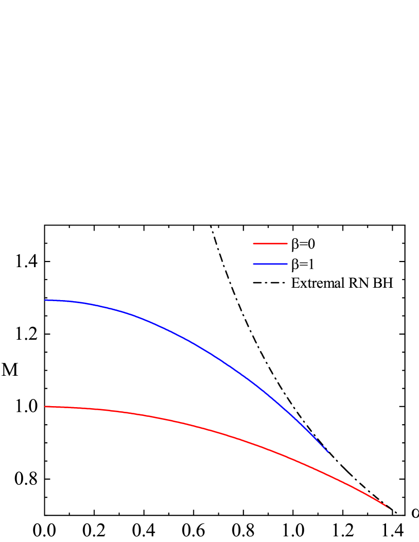
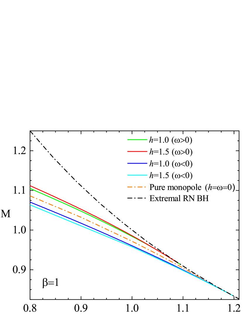
Figure 1: Left panel: The dependence of the ADM mass $M$ of the gravitating monopole on the effective gravitational coupling $\alpha$ is shown for $\beta=0$ and $\beta=1$ at $h=-1$ and $\omega=0$. Right panel: The same dependence is shown for the bounded monopole-fermion system with nonzero (positive and negative) eigenvalues $\omega$ for $\beta=1$ and $h=1,1.5$. For comparison, in both panels, the mass of the extremal Reissner-Nordström black hole of unit charge is also shown.

Generally, the system of mixed order differential equations (8)-(13) can be solved numerically together with constraint imposed by the normalization condition (14). The boundary conditions are found by considering the asymptotic expansion of the solutions on the boundaries of the domain of integration together with the assumption of regularity and asymptotic flatness. Explicitly, we impose

$$\begin{split}N(0)=&1,\quad W(0)=1,\quad H(0)=0,\quad v(0)=0,\quad\partial_{x}u(0)=0,\quad\partial_{x}\sigma(0)=0;\\ N(\infty)=&1,\quad W(\infty)=0,\quad H(\infty)=1,\quad v(\infty)=0,\quad u(\infty)=0,\quad\sigma(\infty)=1\,.\end{split}$$ (19)

Consider first the evolution of the fermion zero mode localized on the self-gravitating BPS monopole. Note that since both the bare mass of the fermion field and the eigenvalue of the Dirac operator are zero, there is no backreaction of the fermions on the monopole, the system of equations (8)-(13) becomes decomposed into 3 familiar coupled equations for self-gravitating monopole [10, 11, 12] and two decoupled equations for the components of the localized fermion mode.

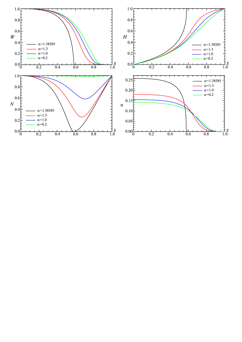
Figure 2: The profile functions of the solutions of the system (8)-(13) in the BPS limit $\beta=0$ are shown as functions of the compactified radial coordinate $\bar{x}=x/(1+x)$ for some set of values of the effective gravitational coupling $\alpha$ at $\omega=0$ and $h=-1$. The spinor component $v$ always remains zero.

The fundamental branch of gravitating BPS monopoles with bounded fermionic zero mode smoothly arise from the flat space configuration (16),(18) as the effective gravitational constant $\alpha$ is increased above zero. This branch reaches a limiting solution at maximal value $\alpha_{\text{max}}=1.403$, here it bifurcates with the short backward branch which leads to the extremal RN black hole with unit magnetic charge, see Fig. 1.

In Fig. 2 we displayed the corresponding solutions for some set of values of the effective gravitational coupling $\alpha$ at $h=-1$ and $\beta=0$. With increasing $\alpha$ the size of the configuration with localized modes is gradually decreasing. As the critical value of $\alpha$ is approached, the minimum of the metric function $N(x)$ tends to zero at $x=x_{\text{cr}}$. The metric becomes splitted into the inner part, $x<x_{\text{cr}}$ and the outer part, $x>x_{\text{cr}}$ separated by the forming hozizon. The Higgs field is taking the vacuum expectation value in exterior of the black hole while the gauge field profile function $W(x)$ trivializes there, so the limiting configuration corresponds to the embedded extremal RN solution (15) with a Coulomb asymptotic for the magnetic field. At the same time, the fermion field becomes absorbed into the interior of the black hole, see Fig. 2.

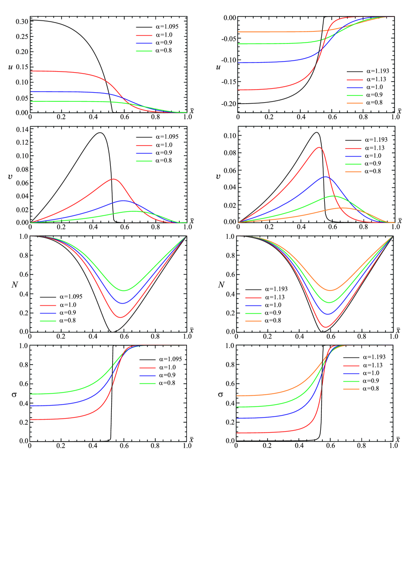
Figure 3: The profiles of the spinor and metric functions of the solutions of the system (8)-(13) are shown as functions of the compactified radial coordinate $\bar{x}=x/(1+x)$ for some set of values of the effective gravitational coupling $\alpha$ at $h=1$, $\beta=1$. The left panel shows the solutions for $\omega>0$ and the right one for $\omega<0$.

Apart from the zero mode, the system of equations (8)-(13) supports a tower of regular normalizable solutions for fermionic modes with $\omega\neq 0,~{}~{}|\omega|<|h/2|$. Here, both components $u$ and $v$ are non-zero, and for $h<0$ they posses at least one node while for $h>0$ they are nodeless. These solutions can be obtained numerically, now we have to solve the full system of coupled differential equations (8)-(13) imposing the boundary conditions (19). Note that this system is not invariant with respect to inversion of the sign of $\omega$. Indeed, it is seen in Figs. 3 and 4, which display the metric components $N(x)\,,\sigma(x)$ and the fields $u(x)\,,v(x)\,,W(x)\,,H(x)$ for some set of values of the gravitational coupling $\alpha$ and fixed $\beta=1$ and $h=1$, that, as $\omega\to+0$ and $\omega\to-0$, the configurations approach the RN limit in a different way.

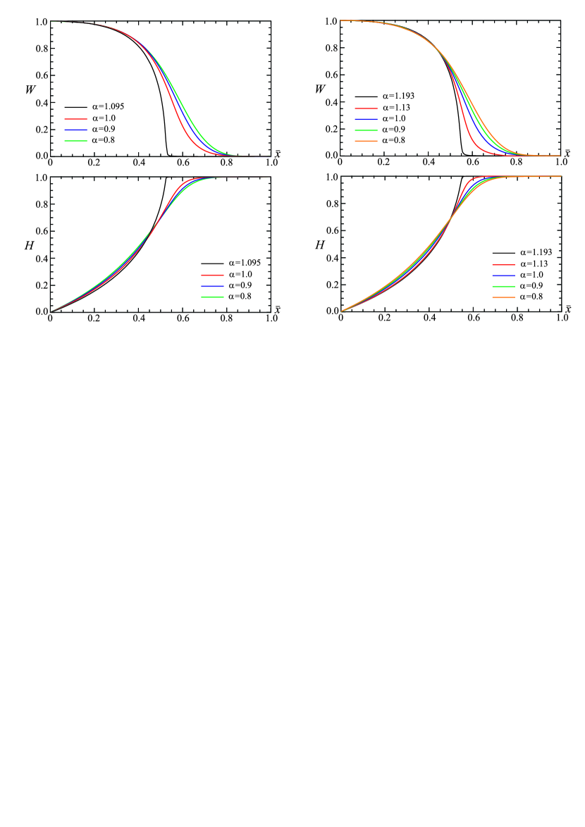
Figure 4: The profiles of the gauge and scalar functions of the solutions of the system (8)-(13) are shown as functions of the compactified radial coordinate $\bar{x}=x/(1+x)$ for some set of values of the effective gravitational coupling $\alpha$ at $h=1$, $\beta=1$. The left panel shows the solutions for $\omega>0$ and the right one for $\omega<0$.

In the flat space limit the fermion mode becomes delocalized as $|\omega|\to|h/2|$, while increasing of the gravitational coupling stabilizes the system. Both the ADM mass of the configuration and the eigenvalue $\omega$, which is defined from the numerical calculations, are decreasing as $\alpha$ increases, see the right panel of Fig. 1. The evolution scenario depends generically on the values of the parameters of the model. For example, setting $\beta=1$ and $h=1$, we observe that there are two branches of solutions which are linked to the negative and positive continuum: they end at the critical value $\alpha_{\text{cr}}\approx 1.095$ as $\omega\to+0$, and at $\alpha_{\text{cr}}\approx 1.193$ as $\omega\to-0$ (cf. Fig. 5 and Table 1). In both cases the configuration reaches the embedded extremal RN solution (15) in a way which is qualitatively similar to that of the BPS monopole with localized fermion zero mode discussed above. As $\alpha$ tends to the critical value, the eigenvalue $\omega$ approaches zero and the fermion field is fully absorbed into interior of the forming black hole.

In Fig. 5 we plot the normalized energy of the localized fermionic states as a function of the Yukawa coupling constant $h$. Having constructed some set of solution for different values of $\alpha$, the following scenario becomes plausible. As the Yukawa coupling increases from zero, while both $\beta$ and $\alpha$ are kept fixed, a branch of normalizible non-zero fermion modes emerges smoothly from the self-gravitating monopole. The energy of the localized fermionic states is restricted as $|\omega|<|h/2|$, as the gravitational coupling remains relatively weak, the modes remain close to the continuum threshold.

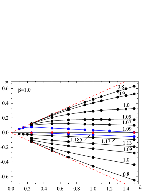
Figure 5: Normalized energy of the localized fermionic states as a function of the Yukawa coupling $h$ for fixed $\beta=1$ and several values of $\alpha$ indicated by the numbers near the curves. The red dashed lines correspond to the continuum threshold $|\omega|=|h/2|$ in the limit $\alpha\to 0$. The blue lines correspond to the curves linked to the extremal RN black hole at some $h_{\text{cr}}$ as $\omega\to 0$. Bold red dots indicate the critical values $h_{\text{cr}}$ given in Table 1.

The spectral flow is more explicit as the coupling $\alpha$ becomes stronger, see Fig. 5. Increase of the Yukawa coupling, which yields the mass of the fermionic states, leads to increase of eigenvalues $\omega$. However, an interesting observation is that at some critical value of the parameter $h$, the energy of the localized mode approaches some maximal value. As the Yukawa coupling continue to grow, the corresponding eigenvalue starts to decrease, it tends to zero as some maximal value $h_{\text{cr}}$. Again, in this limit the configuration approaches the embedded RN solution (15) and the fermion fields are again fully absorbed into interior of the forming black hole. The pattern is illustrated in Fig. 5, where two blue curves display the spectral flow of both positive and negative Dirac eigenvalues $\omega$ for $\alpha=1.09$ and $\alpha=1.185$, respectively. In the limiting case $\omega\to+0$ one has $h_{\text{cr}}\approx 1.5$ (for $\alpha=1.09$) and when $\omega\to-0$ we have $h_{\text{cr}}\approx 0.25$ (for $\alpha=1.185$).

The general scenario is that, depending on the value of the Yukawa coupling constant $h$, there exist a critical value of the gravitational coupling $\alpha_{\text{cr}}$ at which the spectral flow approaches the limit $\omega\to\pm 0$ and the configuration runs to the embedded RN solution (15). Some corresponding values are given in Table 1, and they are also displayed by the bold red dots in Fig. 5. Once again, each particular value of the Yukawa coupling gives rise to two distinct spectral flows approaching the embedded RN solution as $\omega\to\pm 0$ at two different values of $\alpha_{\text{cr}}$.

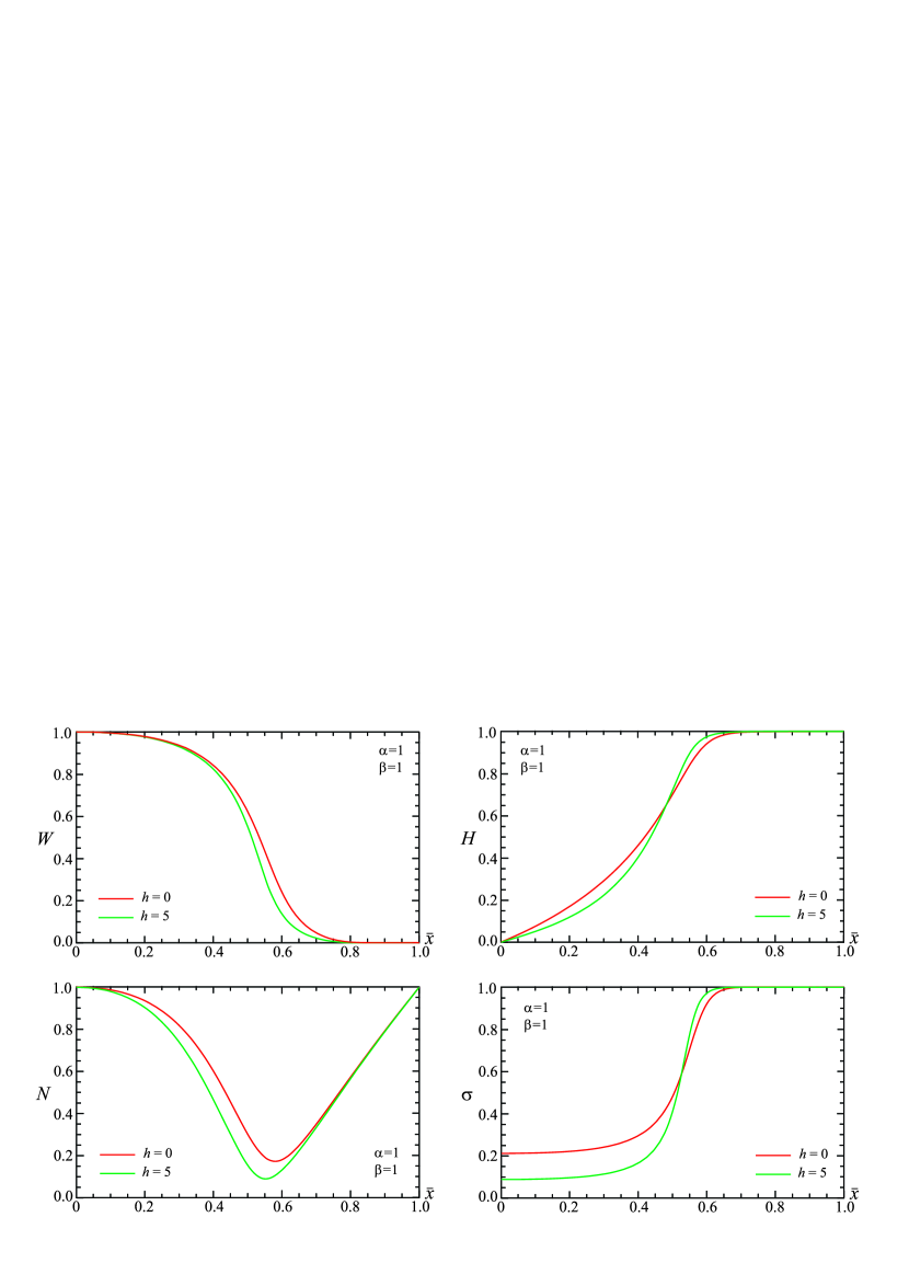
Figure 6: The profile functions of the gauge field $W(x)$, the scalar field $H(x)$, and the metric functions $N(x)$ and $\sigma(x)$ of the gravitating non-BPS monopole ($h=0$) and of the monopole-fermion system ($h=5$) are shown as functions of the compactified radial coordinate $\bar{x}=x/(1+x)$ at $\alpha=1$ and $\beta=1$.

$h$	0.25	0.5	0.7	1.0	1.5
$\alpha_{\text{cr}}(\omega\to+0)$	1.106	1.102	1.10	1.095	1.09
$\alpha_{\text{cr}}(\omega\to-0)$	1.185	1.187	1.191	1.193	1.199

Table 1: Critical values $\alpha_{\text{cr}}$ at which $\omega\to\pm 0$ for some set of values of the Yukawa coupling $h$ (cf. the red bold dots in Fig. 5).

Finally, we note that the system of equations (8)-(13) possesses two characteristic limiting cases, $h\to\infty$ and $\beta\to\infty$. First, for a fixed value of $\beta$ and increasing Yukawa coupling, the backreaction of the localized fermions becomes stronger, the energy of the gravitating bounded fermionic mode increases and the profile functions of the monopole are significantly deformed, see Fig. 6. We observe that an increase of the Yukawa coupling moves the configuration closer to the RN solution (see the bottom plots of Fig. 6). Note that deformations of the configuration caused by its coupling with massive fermion modes may produce a number of interesting effects related with backreaction of the fermions [59, 60, 61, 62].

Secondly, as the scalar field becomes very massive, the core of the monopole shrinks and in the limit $\beta\to\infty$ the Higgs field is taking its vacuum expectation value everywhere in space apart the origin. One can expect that, for the intermediate range of values of $\beta$, the scenario reported above for the $\beta=1$, should persist. Our numerical results confirm that an increase of the scalar coupling $\beta$ decreases the critical value of the Yukawa coupling $h$ at which the configuration approaches the extremal Reissner-Nordström solution. However, for relatively large values of $\beta$, the pattern of evolution of the self-gravitating monopole becomes different [10, 11, 12, 13, 63]. One might expect also that the behavior of the fermion field could be different in the large-$\beta$ regime.

IV Conclusions

The objective of this work is to investigate the fermionic modes localized on the static spherically symmetric self-gravitating non-Abelian monopole in the $SU(2)$ Einstein-Dirac-Yang-Mills-Higgs theory. We have constructed numerically solutions of the full system of coupled field equations supplemented by the normalization condition for the localized fermions, and investigated their properties. We have found that, in addition to the usual zero mode, which always exists for a BPS monopole, there is a tower of gravitationally localized states with nonzero eigenvalues $\omega$, which are linked to the positive and negative continuum. While the fermionic zero mode exists for any negative value of the Yukawa coupling $h$, the massive nodeless modes appear for positive values of $h$. We find that, as we increase the gravitational coupling, the monopole bifurcates with the extremal Reissner-Nordström solution and the fermionic modes become absorbed into the interior of the forming black hole. This scenario is viable for both zero and non-zero fermionic modes. Further, we observe that the Yukawa interaction breaks the symmetry between the localized massive modes with positive and negative eigenvalues. Another observation is that the localized gravitating fermions may deform the monopole affecting the transition to the limiting solution.

The work here should be taken further by considering higher massive localized fermionic states with some number of radial nodes. Another interesting question, which we hope to be addressing in the near future, is to investigate the effect of the bare mass of the fermions, localized on the monopole. Another direction can be related with investigation of properties of charged fermions localized on the self-gravitating dyon. Finally, let us note that there can be several fermionic modes localized by the gravitating monopole. We hope to address these problems in our future work.

Appendix A Definition of the $\gamma^{5}$ matrix in curved (3+1)-dimensional spacetime

The interaction term between the spin-isospin fermions and the Higgs field of non-Abelian self-gravitating monopole in the Lagrangian (2) is

$$-\imath h\bar{\psi}^{i}_{\alpha}\left(\tilde{\gamma}^{5}\right)_{\alpha\beta}\sigma^{a}_{ij}\phi^{a}\psi^{j}_{\beta}\,,$$ (20)

where $\tilde{\gamma}^{5}$ is defined in the curved (3+1)-dimensional spacetime as

$$\tilde{\gamma}^{5}=\frac{1}{4!}E_{\alpha\beta\rho\sigma}\gamma^{\alpha}\gamma^{\beta}\gamma^{\rho}\gamma^{\sigma}=\frac{1}{4!}\sqrt{-g}\epsilon_{\alpha\beta\rho\sigma}e_{a}^{\alpha}e_{b}^{\beta}e_{c}^{\rho}e_{d}^{\sigma}\gamma^{a}\gamma^{b}\gamma^{c}\gamma^{d}=\frac{1}{4!}\sqrt{-g}\left(\epsilon_{\alpha\beta\rho\sigma}\epsilon^{abcd}e_{a}^{\alpha}e_{b}^{\beta}e_{c}^{\rho}e_{d}^{\sigma}\right)\gamma^{5}\,.$$ (21)

Here $E_{\alpha\beta\rho\sigma}=\sqrt{-g}\epsilon_{\alpha\beta\rho\sigma}$ is the Levi-Civita tensor in curved space, $\epsilon_{\alpha\beta\rho\sigma}$ is the Levi-Civita tensor in flat space, and

$$\gamma^{a}\gamma^{b}\gamma^{c}\gamma^{d}=\epsilon^{abcd}\gamma^{5},\quad\gamma^{5}=\imath\gamma^{0}\gamma^{1}\gamma^{2}\gamma^{3}.$$

The expression in the round brackets in (21) is the determinant of the matrix $e^{\alpha}_{a}$:

$$\frac{1}{4!}\epsilon_{\alpha\beta\rho\sigma}\epsilon^{abcd}e_{a}^{\alpha}e_{b}^{\beta}e_{c}^{\rho}e_{d}^{\sigma}=\det\left(e^{\alpha}_{a}\right)=\frac{1}{\sqrt{-g}}.$$

Hence, the interaction term (20) can be written as

$$-\imath h\bar{\psi}^{i}_{\alpha}\left(\gamma^{5}\right)_{\alpha\beta}\sigma^{a}_{ij}\phi^{a}\psi^{j}_{\beta}.$$

References

- [1] M. S. Volkov and D. V. Gal’tsov, Phys. Rept. 319, 1 (1999).
- [2] C. A. R. Herdeiro and E. Radu, Int. J. Mod. Phys. D 24, 1542014 (2015).
- [3] M. S. Volkov, “Hairy black holes in the XX-th and XXI-st centuries,” [arXiv:1601.08230 [gr-qc]].
- [4] M. S. Volkov and D. V. Galtsov, JETP Lett. 50, 346 (1989).
- [5] M. S. Volkov and D. V. Galtsov, Sov. J. Nucl. Phys. 51, 747 (1990).
- [6] P. Bizon, Phys. Rev. Lett. 64, 2844 (1990).
- [7] H. Luckock and I. Moss, Phys. Lett. B 176, 341 (1986).
- [8] S. Droz, M. Heusler, and N. Straumann, Phys. Lett. B 268, 371 (1991).
- [9] P. Bizon and T. Chmaj, Phys. Lett. B 297, 55 (1992).
- [10] K. M. Lee, V. P. Nair, and E. J. Weinberg, Phys. Rev. D 45, 2751 (1992).
- [11] P. Breitenlohner, P. Forgacs, and D. Maison, Nucl. Phys. B 383, 357 (1992).
- [12] P. Breitenlohner, P. Forgacs, and D. Maison, Nucl. Phys. B 442, 126 (1995).
- [13] A. Lue and E. J. Weinberg, Phys. Rev. D 60, 084025 (1999).
- [14] S. Hod, Phys. Rev. D 86, 104026 (2012); [erratum: Phys. Rev. D 86, 129902 (2012)].
- [15] C. A. R. Herdeiro and E. Radu, Phys. Rev. Lett. 112, 221101 (2014).
- [16] C. Herdeiro, I. Perapechka, E. Radu, and Y. Shnir, JHEP 02, 111 (2019).
- [17] Y. Brihaye, B. Hartmann, J. Kunz, and N. Tell, Phys. Rev. D 60, 104016 (1999).
- [18] Y. Brihaye, B. Hartmann, and J. Kunz, Phys. Lett. B 441, 77 (1998).
- [19] B. A. Campbell, M. J. Duncan, N. Kaloper, and K. A. Olive, Phys. Lett. B 251, 34 (1990).
- [20] J. F. M. Delgado, C. A. R. Herdeiro, and E. Radu, Phys. Rev. D 103, 104029 (2021).
- [21] C. Herdeiro, E. Radu, and H. Rúnarsson, Class. Quant. Grav. 33, 154001 (2016).
- [22] C. A. R. Herdeiro and E. Radu, Eur. Phys. J. C 80, 390 (2020).
- [23] J. P. Hong, M. Suzuki, and M. Yamada, Phys. Lett. B 803, 135324 (2020).
- [24] J. Kunz and Y. Shnir, Phys. Rev. D 107, 104062 (2023).
- [25] G. ’t Hooft, Nucl. Phys. B 79, 276 (1974).
- [26] A. M. Polyakov, JETP Lett. 20, 194 (1974).
- [27] T.H.R. Skyrme, Proc. Roy. Soc. Lon. 260, 127 (1961).
- [28] T. H. R. Skyrme, Nucl. Phys. 31, 556 (1962).
- [29] G. Rosen, J. Math. Phys. 9, 996 (1968).
- [30] R. Friedberg, T. D. Lee, and A. Sirlin, Phys. Rev. D 13, 2739 (1976).
- [31] S. R. Coleman, Nucl. Phys. B 262, 263 (1985).
- [32] F. Finster, J. Smoller, and S. T. Yau, Phys. Rev. D 59, 104020 (1999).
- [33] F. Finster, J. Smoller, and S. T. Yau, Phys. Lett. A 259, 431 (1999).
- [34] C. Herdeiro, I. Perapechka, E. Radu, and Y. Shnir, Phys. Lett. B 797, 134845 (2019).
- [35] C. A. R. Herdeiro, A. M. Pombo, and E. Radu, Phys. Lett. B 773, 654 (2017).
- [36] V. Dzhunushaliev and V. Folomeev, Phys. Rev. D 99, 084030 (2019).
- [37] V. Dzhunushaliev and V. Folomeev, Phys. Rev. D 99, 104066 (2019).
- [38] C. Herdeiro, I. Perapechka, E. Radu, and Y. Shnir, Phys. Lett. B 824, 136811 (2022).
- [39] S. R. Dolan and D. Dempsey, Class. Quant. Grav. 32, 184001 (2015).
- [40] B. A. Burrington, J. T. Liu, and W. A. Sabra, Phys. Rev. D 71, 105015 (2005).
- [41] K. Hristov, H. Looyestijn, and S. Vandoren, JHEP 08, 103 (2010).
- [42] S. Ferrara, R. Kallosh, and A. Strominger, Phys. Rev. D 52, R5412 (1995).
- [43] M. F. Atiyah, V. K. Patodi, and I. M. Singer, Math. Proc. Cambridge Phil. Soc. 77, 43 (1975).
- [44] J. Maldacena, JHEP 04, 079 (2021).
- [45] R. F. Dashen, B. Hasslacher, and A. Neveu, Phys. Rev. D 10, 4130 (1974).
- [46] R. Jackiw and C. Rebbi, Phys. Rev. D 13, 3398 (1976).
- [47] C. Caroli, P.G. De Gennes, and J. Matricon, Phys. Lett. 9, 307 (1964).
- [48] R. Jackiw and P. Rossi, Nucl. Phys. B 190, 681 (1981).
- [49] J. R. Hiller and T. F. Jordan, Phys. Rev. D 34, 1176 (1986).
- [50] S. Kahana, G. Ripka, and V. Soni, Nucl. Phys. A 415, 351 (1984).
- [51] V. A. Rubakov, Nucl. Phys. B 203, 311 (1982).
- [52] C. G. Callan, Jr., Phys. Rev. D 26, 2058 (1982).
- [53] R. Jackiw and C. Rebbi, Phys. Rev. Lett. 36, 1116 (1976).
- [54] E. B. Bogomolny, Sov. J. Nucl. Phys. 24, 449 (1976).
- [55] M. K. Prasad and C. M. Sommerfield, Phys. Rev. Lett. 35, 760 (1975).
- [56] Y. M. Shnir, Magnetic Monopoles (Springer, 2005).
- [57] F. A. Bais and R. J. Russell, Phys. Rev. D 11, 2692 (1975).
- [58] Y. M. Cho and P. G. O. Freund, Phys. Rev. D 12, 1588 (1975); [erratum: Phys. Rev. D 13, 531 (1976)].
- [59] I. Perapechka, N. Sawado, and Y. Shnir, JHEP 10, 081 (2018).
- [60] I. Perapechka and Y. Shnir, Phys. Rev. D 99, 125001 (2019).
- [61] V. Klimashonok, I. Perapechka, and Y. Shnir, Phys. Rev. D 100, 105003 (2019).
- [62] I. Perapechka and Y. Shnir, Phys. Rev. D 101, 021701 (2020).
- [63] J. Kunz, U. Neemann, and Y. Shnir, Phys. Rev. D 75, 125008 (2007).