On the Distribution of Probe Traffic Volume Estimated from Their Footprints

Abstract

Collecting traffic volume data is a vital but costly piece of transportation engineering and urban planning. In recent years, efforts have been made to estimate traffic volumes using passively collected probe data that contain spatiotemporal information. However, the feasibility and underlying principles of traffic volume estimation based on probe data without pseudonyms have not been examined thoroughly. In this paper, we present the exact distribution of the estimated probe traffic volume passing through a road segment based on probe point data without trajectory reconstruction. The distribution of the estimated probe traffic volume can exhibit multimodality, without necessarily being line-symmetric with respect to the actual probe traffic volume. As more probes are present, the distribution approaches a normal distribution. The conformity of the distribution was demonstrated through numerical and microscopic traffic simulations. Theoretically, with a well-calibrated probe penetration rate, traffic volumes in a road segment can be estimated using probe point data with high precision even at a low probe penetration rate. Furthermore, sometimes there is a local optimum cordon length that maximises estimation precision. The theoretical variance of the estimated probe traffic volume can address heteroscedasticity in the modelling of traffic volume estimates.

1 Introduction

Traffic volume is a fundamental element of transportation engineering (Greenshields, 1934), urban planning, real estate valuation, air pollution models (Luria et al., 1990; Okamoto et al., 1990), wildlife protection (Seiler and Helldin, 2006), and marketing (Alexander et al., 2005). Traffic counts are typically performed at fixed locations using equipment such as pneumatic tubes, loop coils, radars, ultrasonic sensors, video cameras, and light detection and ranging (LiDAR) systems (Zhao et al., 2019). While conventional traffic counts are believed to have acceptable precision, traffic counts at fixed locations are constrained in space, time, and budget. For this reason, average annual daily traffic (AADT), which is one of the basic traffic metrics in traffic engineering, is often estimated based on 24- or 48-hour traffic counts with temporal adjustments (Jessberger et al., 2016; Krile and Schroeder, 2016; Ritchie, 1986). Nevertheless, this scalability constraint still places transportation professionals in a leash. For example, researchers have pointed out a lack of reliable traffic volume data in substantive road safety analyses (Chen et al., 2019; El-Basyouny and Sayed, 2010; Mitra and Washington, 2012; Zarei and Hellinga, 2022).

To maximise the value of limited numbers of traffic counts, extensive research efforts have been devoted to developing traffic volume estimation methods focused on calibration and its accuracy. Such approaches include travel demand modelling (Zhong and Hanson, 2009), spatial kriging (Selby and Kockelman, 2013), support vector machines (Sun and Das, 2015), linear and logistic regressions (Apronti et al., 2016), geographically weighted regression (Pulugurtha and Mathew, 2021), locally weighted power curves (Chang and Cheon, 2019), and clustering (Sfyridis and Agnolucci, 2020).

1.1 Probe Data in Traffic Volume Estimation

With the advancements in information technology, expectations for traffic volume availability have increased. In the United States, for example, the Highway Safety Improvement Program (HSIP) asks state departments of transportation to prepare traffic volume data even on low-volume roads (Federal Highway Administration, 2016). As mobile devices compatible with global navigation satellite systems (GNSSs) have spread throughout our daily lives, opportunities to estimate traffic volumes based on passively collected location data have gained industry attention (Caceres et al., 2008; Harrison et al., 2020). Road agencies have started exploring the feasibility of using probe data to estimate traffic volumes (Codjoe et al., 2020; Fish et al., 2021; Krile and Slone, 2021; Macfarlane and Copley, 2020; Zhang et al., 2019) because probe volumes and traffic volumes tend to be positively correlated. In proprietary products providing AADT estimations, reports have found negative correlations between true traffic volumes and estimation accuracy as measured by percentage errors (Barrios and Casburn, 2019; Roll, 2019; Schewel et al., 2021; Tsapakis et al., 2020; Tsapakis et al., 2021; Turner et al., 2020; Yang et al., 2020).

Machine learning methods have become popular calibration tools for traffic volume estimation by using probe location data. For instance, Meng et al. (2017) and Zhan et al. (2017) applied spatio-temporal semi-supervised learning and an unsupervised graphical model, respectively, to taxi trajectories in Chinese cities to estimate citywide traffic volumes. With a Maryland probe dataset, Sekuła et al. (2018), for example, showed that neural networks could significantly improve estimation accuracy. In Kentucky, Zhang and Chen (2020) used annual average daily probes (AADP) and betweenness centrality to estimate AADTs across the state. Using random forest, they found that an AADP of 53 was the lower threshold for having a mean absolute percentage error (MAPE) of less than 20 % to 25 %. Machine learning methods, including support vector machines and gradient boosting, provide practical solutions for calibrating high-dimensional data and improving estimation accuracy (Schewel et al., 2021).

1.2 Types of Probe Data

Figure 1 illustrates different types of probe data: point data (Figure 1a) and line data (Figure 1b). Point data refer to data that contain information to identify a point location (e.g., geographic coordinates) on a surface, such as the Earth’s ellipsoid. Location data are usually first recorded and stored as point data. In contrast, line data, also called trajectories, paths, or routes, consist of a series of point data of an entity connected chronologically (Marković et al., 2019). Conventional traffic counts require information on passing objects over a cross-section at a fixed location. With probe data, one can count the number of probes passing through a specific location based on trajectories reconstructed from point data (e.g., GPS Exchange Format (GPX)) when the point data meet all of the following conditions:

• Each probe has a pseudonym (e.g., device identifier).

• Each point data has a timestamp in the ordinal scale or a higher level of measurement.

• The recording interval is small enough to determine a route.

Figure 1: Illustrated virtual cordons over probe point data and line data (reconstructed trajectories).

In other words, data that meet these conditions have less anonymity because one can track each probe’s locations and time simultaneously (de Montjoye et al., 2013). In fact, all of the aforementioned studies used line data of probes to estimate traffic volumes. However, some point data are unsuitable for the precise reconstruction of line data. Sparsely recorded probe data are an example (Sun et al., 2013). In addition, agencies might not be able to obtain detailed line data in which they can identify a probe’s geographic coordinates and timestamps at once, depending on privacy regulations and data providers’ policies.

To relax such constraints on probe data availability in traffic volume estimation, this paper presents a method for estimating probe traffic volumes using passively collected point location data without route reconstruction. In addition, we describe the exact distribution of the unbiased estimator with which one can assess the estimation precision. On the other hand, we will hardly tap into detailed calibration methods against known traffic volumes, which ultimately influences traffic volume estimation accuracy. In the following sections, we derive analytical relationships between traffic variables and estimated probe counts with example calculations. Numerical and microscopic traffic simulations further demonstrate the conformity of the model. Finally, we discuss the characteristics, limitations, applications, and opportunities of the model.

2 Theory

This section describes the problem, provides our findings with proofs, and offers illustrative examples. We adhere to the International System of Units throughout the paper unless stated otherwise.

2.1 Problem Statement

We define a “probe” as a device that records its position as point data in the Earth’s spatial reference system (e.g., geographic coordinates). For instance, a smartphone and connected vehicle can be a probe. Let $m\ \{m\in\mathbf{Z}^{nonneg}\}$ and $\hat{m}$ denote the number of probes passing through a unit segment during an observation period and its estimator, respectively. We present the distribution of $\hat{m}$ under the following conditions.

Assume that each probe traverses the Earth’s surface at a speed of $S$ $\{S\in\mathbf{R}^{+}\}$ m/s, where $S$ is an independent and identically distributed (i.i.d.) continuous random variable. We denote the realised value of $S$ as $s$ $\{s\in\mathbf{R}^{+}\}$. Let $g(s)$ $\{g(s)\in\mathbf{R}^{nonneg}\mid 0\leq g(s);\displaystyle\int_{0}^{\infty}g(s)\mathrm{d}s=1\}$ be the probability density function (PDF) of the probe speed population. The population of $s$ is a hypothetical infinite group of $s$. Therefore, the possibility that multiple probes are carried by one vehicle at the same $s$ is already considered in $g(s)$ as a part of the distribution. All probes share the same data recording interval $t$ $\{t\in\mathbf{R}^{+}\}$ s. In a uniform motion, each probe records its position as point data (i.e., “footprints”) at an interval of $t$ s. The probe speed is recorded during this process. Probe identifiers $i$ or detailed timestamps are not necessarily recorded, but data points have at least nominal information to identify a recorded time range of interest (e.g., a label of “July 2023”). We assume that there are no errors or failures in the positioning or recording.

After the probe point location data are recorded, an analyst draws a $d$-m virtual cordon ($\{d\in\mathbf{R}^{+}\}$) over the data measured along the road segment of interest. This spatial data cropping procedure makes each probe record its first location in the virtual cordon at a uniformly distributed random timing within any nonnegative seconds less than $t$ after a probe enters the cordon. The analyst may extract data within the time range of interest, as needed. The virtual cordon will contain $n\ \{n\in\mathbf{Z}^{nonneg}\}$ data points at a speed of $s_{a}$ where $a\ \{a\in\mathbf{Z}^{nonneg}\mid a\leq n\}$ is a record identifier. Figure 2 shows an example of a virtual cordon containing eight data points. Although the figure distinguishes the two probes, this work does not assume that analysts have information to identify individual probes.

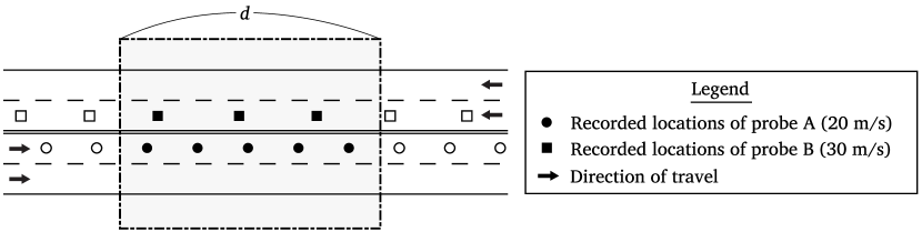
Figure 2: An illustrated virtual cordon over point data ($m=2$).

2.2 Unbiased Estimator of $m$

Lemma 1.

If we define $\hat{m}$ as

$$\hat{m}=\frac{t}{d}\sum_{a=1}^{n}s_{a},\forall m,d,t,n,s$$ (1)

$\hat{m}$ is an unbiased estimator of the true probe traffic volume $m$ (Equation 2).

$$\mathrm{E}[\hat{m}]=m,\forall m$$ (2)

Proof.

Because uniform motion is assumed, $s_{i}=s_{a}$ within any probe and $s_{i}t$ is the distance along a cordon the $i$th probe traverses in $t$ s. Using $n_{i}$ as the number of data points within a cordon from the probe, Equation 1 can be reduced to

$$\hat{m}=\displaystyle\frac{ts_{i}n_{i}}{d}$$ (3)

for the $i$th probe. In Equations 1 and 3, $n_{i}$ can be broken down into $n_{i}=\tilde{n}_{i}+K_{i}$ where $\tilde{n}_{i}$ $\{{\tilde{n}\in\mathbf{Z}^{nonneg}}\}$ is the minimum number of data points that could be recorded in the virtual cordon. It is calculated with the floor function as

$$\tilde{n}_{i}=\left\lfloor\frac{d}{s_{i}t}\right\rfloor$$ (4)

Here, $K_{i}$ is a Bernoulli random variable representing the number of additional data points per probe $\{{K\in\mathbf{\{}0,1\}}\}$ observed in addition to $\tilde{n}_{i}$ data points. Because uniform motion is assumed and a probe leaves its first record in the cordon at a random time at $t$ s or before once the probe enters the cordon. Naturally, an additional data point is recorded at the probability of the fractional part of $d/(s_{i}t)$. When we define the fractional part as $p_{i}$ $\{{p\in\mathbf{R}^{nonneg}\mid 0\leq p<1}\}$,

$$p_{i}=\frac{d}{s_{i}t}\mod 1$$ (5)

Because $K_{i}$ follows the Bernoulli distribution $Ber(p_{i})$, its expected value $\mathrm{E}[K_{i}]$ is $p_{i}$. From Equations 3, 4, and 5, $\mathrm{E}[\hat{m}]$, the expected value of $\hat{m}$, is

$$\mathrm{E}[\hat{m}]=\frac{s_{i}t}{d}\left[\left\lfloor\frac{d}{s_{i}t}\right\rfloor+\left(\frac{d}{s_{i}t}\mod 1\right)\right]=1$$ (6)

when $m=1$. Accordingly, $\mathrm{E}[\hat{m}]=m$ for any $m$. Therefore, $\hat{m}$ is an unbiased estimator of $m$. ∎

2.2.1 Example 1

We assume $d=100$ and $t=1$ in Figure 2. The expected number of records within the segment from probe B ($s_{i}=30$) is $100/(30\cdot 1)\approx 3.333$; therefore, at least three records are observed (i.e., $\tilde{n}=3$). Since it is impossible to observe 3.333 records, one more record is observed at a probability of approximately 0.333 (i.e., $p_{i}\approx 0.333$). In Figure 2, $m=2$, $\mathrm{E}[\hat{m}]=2$ and $\hat{m}=1.9$. If the cordon had contained the data points only from probe A, $m=1$, $\mathrm{E}[\hat{m}]=1$ and $\hat{m}=1$. If the cordon had included the data points only from probe B, $m=1$, $\mathrm{E}[\hat{m}]=1$ and $\hat{m}=0.9$.

2.3 Variance of $\hat{m}$

Lemma 2.

When we denote the variance of $\hat{m}$ as $\mathrm{Var}[\hat{m}]$:

$$\mathrm{Var}[\hat{m}]=\frac{mt^{2}}{d^{2}}\int_{0}^{\infty}b(s,d,t)g(s)\mathrm{d}s$$ (7)

where

$$b(s,d,t)=s^{2}p(1-p)=s^{2}\left(\frac{d}{st}\mod 1\right)\left[1-\left(\frac{d}{st}\mod 1\right)\right]$$ (8)

Proof.

The variance of $\hat{m}$ originates from the discreteness of the number of recorded data points, namely, the Bernoulli random variable $K$. From Equation 3 and the multiplication rule of probability, $\mathrm{Var}[\hat{m}\mid S=s_{i}]$ is proportional to the variance of the Bernoulli distribution $p(1-p)$ multiplied by the scaling factor $st/d$ raised to a power of 2. Because $S\sim g(s)$, integrating $s^{2}t^{2}p(1-p)g(s)/d^{2}$ over $s$ gives the variance of $\hat{m}$ per probe. Because $S$ is assumed to be i.i.d., $\mathrm{Var}[\hat{m}]\propto m$ from the additivity of variances. ∎

2.3.1 Example 2

Hereafter, we use a finite mixture of normal distributions by Park et al. (2010) as $g(s)$ unless stated otherwise. The speed distribution had been fitted to data collected on Interstate Highway 35 (I-35) in Texas. It is comprised of four normal distributions $N(\upmu,\upsigma^{2})$ defined by $\upmu=(27.042,24.000,9.394,4.294)$, $\upsigma=(1.831,4.797,3.167,1.686)$, $w=(0.647,0.223,0.055,0.074)$, and $\displaystyle\sum w_{j}=1$ where $\upmu\ \{\upmu\in\mathbf{R}\}$ is a tuple (i.e., a finite ordered list) of mean speed in m/s, $\upsigma\ \{\upsigma\in\mathbf{R}^{nonneg}\}$ is a tuple of standard deviation in m/s before truncation, and $w\ \{w\in\mathbf{R}^{nonneg}\,|\,w\leq 1\}$ defines the proportions of the normal distributions within the mixture. The distribution was truncated at $s$ = 0 and $s$ = 40. The resulting $g(s)$ is a mixture of four truncated normal distributions, defined by the following equations (Figure 3a):

$$g(s\mid\upmu,\upsigma,0,40)=\begin{cases}\displaystyle\sum\limits_{j=1}^{4}w_{j}\uppsi(s\mid\upmu_{j},\upsigma_{j},0,40),&0<s\leq 40\\ 0,&\text{otherwise}\end{cases}$$ (9)

where $\upalpha<\upbeta$, $0<\upsigma$, and

$$\uppsi(x\mid\upmu,\upsigma,\upalpha,\upbeta)=\frac{\upphi\displaystyle\left(\frac{x-\upmu}{\upsigma}\right)}{\upsigma\displaystyle\left[\Phi\displaystyle\left(\frac{\upbeta-\upmu}{\upsigma}\right)-\Phi\displaystyle\left(\frac{\upalpha-\upmu}{\upsigma}\right)\right]}\\$$ (10)

$$\upphi(x)=\displaystyle\frac{e^{\displaystyle\left(\frac{-x^{2}}{2}\right)}}{\sqrt{2\uppi}}$$ (11)

$$\Phi(x)=\frac{1}{2}\displaystyle\left[1+\operatorname*{erf}\displaystyle\left(\frac{x}{\sqrt{2}}\right)\right]\\$$ (12)

Assuming $d=300$ and $t=4$, Figure 3b displays $4^{2}/300^{2}\cdot b(s,300,4)$, the variance in the estimated probe traffic volume as a function of $s$ (Equation 8). If $S$ were uniformly distributed between 0 and 40 (i.e., $S\sim U(0,40]$), the area under the function in Figure 3b would have been proportional to the variance of the estimated probe traffic volume (i.e., $\mathrm{Var}[\hat{m}\mid S=s_{i}]$). Here, we want to weigh $4^{2}/300^{2}\cdot b(s,300,4)$ by $g(s)$ because $S\sim g(s)$. The operation gives Figure 3c, where the area under the function, 0.019, is the theoretical variance of $\hat{m}$ from a probe (Equation 7).

Figure 3: Variance derivation when $d$ = 300, $t$ = 4, and $S\sim g(s)$.

2.4 Shape of $\hat{m}$

Theorem 1.

Let $u$ be a nonnegative integer $\{{u\in\mathbf{Z}^{nonneg}}\}$ that operationally substitutes $\tilde{n}$. With the previously defined variables and a function, the PDF of $\hat{m}$ is given as $f(\hat{m};m)$:

$$f(\hat{m};m)=f^{\prime*m}(\hat{m})$$ (13)

where $f^{\prime*m}(\hat{m})$ denotes $m$-fold self-convolution of $f^{\prime}(\hat{m})$. The function $f^{\prime}(\hat{m})$ is defined as

$$f^{\prime}(\hat{m})=\displaystyle\sum_{u=0}^{\infty}\sum_{k=0}^{1}h(\hat{m};t,d,u,k)$$ (14)

where

$$h(\hat{m};t,d,u,k)=\begin{cases}\displaystyle g\left(\frac{d\hat{m}}{t(u+k)}\right)\frac{p^{k}(1-p)^{1-k}d}{t(u+k)},&(u=0\land k\neq 0)\lor\left(u\neq 0\land\displaystyle\frac{u+k}{u+1}<\hat{m}\leq\displaystyle\frac{u+k}{u}\right)\\ 0,&\text{otherwise}\end{cases}$$ (15)

Proof.

From Equations 4 and 5, $s$ uniquely determines $\tilde{n}$ and $p$ once $d$ and $t$ are determined. In addition, any single $s$ has a mutually exclusive set of $k$ as the outcome of a Bernoulli trial. In Equation 3, $\hat{m}$ is a linear function of $s$ with slope $t(\tilde{n}+k)/d$. Because the probe speed $S$ is i.i.d., the summation of all relative frequencies for possible occurrences of $\tilde{n}$ and $k$ by $\hat{m}$ gives the PDF of $\hat{m}$; therefore, the PDF of $\hat{m}$ contains the joint probability function $g(s)p^{k}(1-p)^{1-k}$. In Equations 14 and 15, $u$ substitutes for $\tilde{n}$. Let $x$ be a nonnegative real number $\{{x\in\mathbf{R}^{nonneg}}\}$ and $\updelta$ be an infinitesimal interval. The probability that $\hat{m}$ takes a value in the interval $(x,x+\updelta]$ is calculated by integrating the PDF of $\hat{m}$ over the interval. From Equation 3, $m=0$ when $u+k=0$; otherwise, the interval of $s$ corresponding to $(x,x+\updelta]$ is $(s,s+\updelta^{\prime}]$ = $\displaystyle\left(dx/\left[t(u+k)\right],dx/\left[t(u+k)\right]+\updelta d/\left[t(u+k)\right]\right]$, where $dx/\left[t(u+k)\right]$ is $s$ as a function of $\hat{m}$ and $d/\left[t(u+k)\right]$ is the reciprocal of the slope of $\hat{m}$ as a function of $s$ (e.g., Figure 4). However, the interval of $s$ must be constant regardless of $\hat{m}$ in the PDF of $\hat{m}$ because $\hat{m}$ results from $S$, but not vice versa. Therefore, the joint probability of $u$ and $k$, in fact, must be multiplied by $d/\left[t(u+k)\right]$, which is the reciprocal of the slope of $s$ as a function of $\hat{m}$. When $S$ is i.i.d., $\hat{m}$ is also i.i.d. (Equation 3). Hence, the PDF of $\hat{m}$ emerges as an $m$-fold self-convolution of the PDF where $m=1$ (Equation 13). ∎

Corollary 1.

As $m$ approaches infinity, the shape of $f(\hat{m};m)$ converges to that of a normal distribution:

$$\lim_{{m\to\infty}}f(\hat{m};m)=N\left(m,\frac{mt^{2}}{d^{2}}\int_{0}^{\infty}b(s,d,t)g(s)\mathrm{d}s\right)$$ (16)

Proof.

Because $\hat{m}$ is i.i.d., Equation 16 is derived from the classical central limit theorem on lemmata 1 and 2. ∎

2.4.1 Example 3

Assuming $d=300$ and $t=4$, Figure 4 plots Equation 3 (i.e., when $m=1$). The combinations of $\tilde{n}$ and $k$ fall into an infinite periodic pattern along the $s$-axis because $\tilde{n}$ increases towards infinity as $s$ approaches 0. Because $S\sim g(s)$, we want to take the relative frequency of speed and each $k$ by multiplying the probability mass function (PMF) of $Ber(p)$ by $g(s)$. After this operation, we obtain the overall frequency of the combination of $\tilde{n}$ and $k$ by $s$ (Figure 5).

Figure 4: $\hat{m}$ as a function of $s$ and $k$ when $d$ = 300, $t$ = 4, and $m$ = 1.

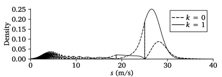
Figure 5: The PMFs of $Ber(p)$ weighted by $g(s)$ as a function of $s$ and $k$ when $d$ = 300 and $t$ = 4.

From Figure 4, it is apparent that the density in an interval of $\hat{m}$ can emerge from more than one combination of $\tilde{n}$ and $k$, which have different slopes for $\hat{m}$ with respect to $s$. Therefore, an infinitesimal interval of $\hat{m}$ can have different cardinalities of the frequencies projected from the $s$-axis; thus, we must consider the cardinality of $\hat{m}$. For example, the length of an infinitesimal interval of $\hat{m}$ corresponding to any interval between $s=25$ and $s=37.5$ in Figure 4 is 50 % longer when $k=1$ than when $k=0$. Because we are interested in the PDF of $\hat{m}$, we must normalise the value using the cardinality of $\hat{m}$. This operation can be performed by dividing the relative frequency given the combination of $\tilde{n}$ and $k$ by each slope $t(\tilde{n}+k)/d$ before summation. Equation 14 results in the PDF in Figure 6 in this example.

Figure 6: The PDF of $\hat{m}$ when $m=1,d=300,$ and $t=4$.

2.5 Optimum Cordon Length

Equation 7 tells that $d$ determines $\mathrm{Var}[\hat{m}]$ when $t$ and $g(s)$ are already fixed. Considering that $d$ is often the only parameter that an analyst can control, the art of estimation error minimisation lies in setting a good cordon length $d$. That said, how long should $d$ be in what conditions? Modelling the relationships between $\hat{m}$ and the other variables gives us a hint on choosing a good cordon length $d$.

Corollary 2.

Let $\max(d)$ denote the maximum feasible $d$ within a given segment. When $\max(d)$ exists, there can be a cordon length $d$ shorter than $\max(d)$ that minimises the precision of estimating $m$. Such $d$ can be sought by $\displaystyle\operatorname*{argmin}_{0<d\leq\max(d)}obj(d)$ where $obj(d)$ is an objective function such as the variance-to-mean ratio (VMR)

$$\mathrm{VMR}[\hat{m}]=\frac{\mathrm{Var}[\hat{m}]}{\mathrm{E}[\hat{m}]}=\frac{t^{2}}{d^{2}}\int_{0}^{\infty}b(s,d,t)g(s)\mathrm{d}s$$ (17)

or the coefficient of variation (CV)

$$\mathrm{CV}[\hat{m}]=\frac{\sqrt{\mathrm{Var}[\hat{m}]}}{\mathrm{E}[\hat{m}]}=\frac{t}{d}\sqrt{\frac{1}{m}\int_{0}^{\infty}b(s,d,t)g(s)\mathrm{d}s}$$ (18)

Proof.

Assume that Corollary 2 is false. In other words, assume that $\mathrm{CV}[\hat{m}]$ always monotonically decreases as $d$ increases. When $m=1$, $t=4$ and $S\sim g(s)$ defined by Equations 9-12, $\mathrm{CV}[\hat{m}]=0.310$ when $d=150$ whereas $\mathrm{CV}[\hat{m}]=0.230$ when $d=110$. Because there is a counterexample to the assumed proposition that Corollary 2 is false, Corollary 2 is true. ∎

2.5.1 Example 4

This example provides graphical descriptions of the proof of Corollary 2. Figure 7 displays an example: $b(s,d,4)g(s)$ and $4^{2}/d^{2}\cdot b(s,d,4)g(s)$ as functions of $s$ and $d$ when $S\sim g(s)$. In Figure 7a, $b(s,d,t)g(s)$ has a periodic pattern along the $d$-axis. Figure 7b is an extension of Figure 3c to the $d$-axis, where $b(s,d,t)g(s)$ is scaled by $t^{2}/d^{2}$ to plot Equation 17 when $m=1$). Because $\mathrm{VMR}[\hat{m}]$ is inversely proportional to $d^{2}$, a larger $d$ tends to result in a better precision in $\hat{m}$. This is intuitive considering $\mathrm{Var}[\hat{m}]$ arises from the discreteness of the observed number of records. The ratio of the additional number of records $K$, a Bernoulli random variable, to the total number of records $n$ decreases as the cordon captures more data points, owing to a larger $d$.

However, VMR$[\hat{m}]$ or CV$[\hat{m}]$ does not always exhibit a monotonic decrease over $d$. As seen in Figure 8a, the non-monotonicity of $\mathrm{CV}[\hat{m}]$ as a function of $d$ indicates the potential existence of $d$ that locally minimises the VMR or CV when the maximum $d$ exists. When some road geometry dictates the maximum $d$ to be 150 m (e.g., a 150-m road segment immediately bounded by intersections, beyond which traffic volumes can be different) in the condition of Figure 8a, it would be better to set 110-m $d$ ($CV=23.048\ \%$) than trying to set 150-m $d$ ($CV=30.999\ \%$). Figure 8b plots CV$[\hat{m}]$ as a function of $t$ when $d=300$. CV$[\hat{m}]$ tends to increase as $t$ increases, but this relationship is not always monotonic.

Figure 7: Surface plots of $b(s,d,4)g(s)$ and $\displaystyle\frac{16}{d^{2}}b(s,d,4)g(s)$.

Figure 8: CV[$\hat{m}$] as a function of $d$ and $t$ when the other variables are fixed.

3 Simulations

To supplement discussions, we illustrate the proposed model through numerical and microscopic traffic simulations.

3.1 Particle Simulations

We compared numerically simulated distributions of $\hat{m}$ with the theoretical distributions of $\hat{m}$.

3.1.1 Method

In Julia 1.8.5, the number of probe footprints was modelled as a series of particles with independent uniform linear motion along a road segment. In this experiment, the emergence of binomial distributions (Equation 5) was assumed trivial. The Distributions.jl package was used to generate statistical distributions under the following two scenarios: scenario 1 ($d=300$ and $t=4$) and scenario 2 ($d=40$ and $t=1$). In each scenario, $m\in\{1,2,4,8\}$ and $S\sim g(s)$ as shown in Figure 3a. We performed one million simulations using Equation 1 for each combination of scenarios and $m$.

3.1.2 Results

Table 1 exhibits the descriptive statistics of simulations and theory, while Figure 9 shows the histograms of simulated $\hat{m}$ and theoretical PDFs of $\hat{m}$ calculated by Equation 13. The simulation results showed a good match in descriptive statistics between simulated values and theoretical values.

As seen in Figure 9, $\hat{m}$ distributes around $m$, but the PDFs are not necessarily line-symmetric with respect to $\hat{m}=m$. The PDFs approached normal distributions as $m$ increased.

Table 1: Descriptive Statistics of $\hat{m}$ in Simulations and Theory

Scenario	$m$	Item	E[$\hat{m}$]	Var[$\hat{m}$]	CV[$\hat{m}$]
1	1	Simulated	1.000	0.019	0.137
		Theoretical	1	0.019	0.137
	2	Simulated	2.000	0.037	0.097
		Theoretical	2	0.037	0.097
	3	Simulated	4.000	0.075	0.068
		Theoretical	4	0.075	0.068
	4	Simulated	8.000	0.150	0.048
		Theoretical	8	0.149	0.048
2	1	Simulated	1.000	0.088	0.297
		Theoretical	1	0.088	0.297
	2	Simulated	2.000	0.177	0.210
		Theoretical	2	0.177	0.210
	3	Simulated	4.000	0.353	0.148
		Theoretical	4	0.353	0.149
	4	Simulated	7.999	0.706	0.105
		Theoretical	8	0.706	0.105

Figure 9: Histograms of Simulated $\hat{m}$ and PDFs of $\hat{m}$.

3.2 Regressions on Microscopic Traffic Simulations

To develop traffic volume estimation models, $\hat{m}$ is compared to known traffic volumes to calibrate the ratio of traffic volumes to the estimated probe traffic volumes. Here, we briefly illustrate how the theoretical variance of $\hat{m}$ can improve traffic volume estimation accuracy through a fitter model.

3.2.1 Method

Table 2: Traffic Volume Data Used in Regressions

Site number	Modelled speed distribution	ADT	$m$	$d$	VMR[$\hat{m}$]
	(m/s)			(m)
4945	$N(26.82,5.00)$	763	107	14	0.916
4953	$N(26.82,5.00)$	27	4	53	0.028
4961	$N(26.82,5.00)$	19	3	64	0.035
4977	$N(26.82,5.00)$	34	5	56	0.025
4985	$N(26.82,5.00)$	618	87	52	0.030
5001	$N(26.82,5.00)$	751	105	62	0.033
5025	$N(26.82,5.00)$	706	99	25	0.092
5057	$N(26.82,5.00)$	83	12	27	0.059
5065	$N(26.82,5.00)$	275	39	46	0.066
5081	$N(26.82,5.00)$	52	7	56	0.025
5089	$N(26.82,5.00)$	38	5	35	0.116
5097	$N(13.41,5.00)$	183	26	41	0.019
5113	$N(26.82,5.00)$	110	15	10	1.682
5121	$N(13.41,5.00)$	539	75	41	0.019
5129	$N(13.41,5.00)$	353	49	62	0.008
5145	$N(26.82,5.00)$	448	63	20	0.341
5185	$N(26.82,5.00)$	668	94	53	0.028
5201	$N(13.41,5.00)$	96	13	21	0.086
5217	$N(26.82,5.00)$	277	39	39	0.111
5225	$N(26.82,5.00)$	232	32	66	0.035
9193	$N(26.82,5.00)$	48	7	57	0.026
9201	$N(26.82,5.00)$	8	1	64	0.035
9209	$N(26.82,5.00)$	63	9	17	0.578
9233	$N(26.82,5.00)$	289	40	52	0.030
9249	$N(26.82,5.00)$	216	30	7	2.831
9257	$N(26.82,5.00)$	820	115	57	0.026
9281	$N(13.41,5.00)$	226	32	46	0.014
9289	$N(26.82,5.00)$	446	62	25	0.092
9297	$N(26.82,5.00)$	52	7	70	0.030
9305	$N(26.82,5.00)$	135	19	49	0.045
9313	$N(26.82,5.00)$	221	31	50	0.039
9321	$N(26.82,5.00)$	121	17	41	0.101
9329	$N(26.82,5.00)$	41	6	28	0.059
9353	$N(26.82,5.00)$	46	6	31	0.090

Note. — Speed distributions had been truncated at $s=0$ and $s=60$. The modelled speed distributions did not necessarily match the actual speed distribution at each site in Hudspeth County.

We used PTV Vissim 11.00-02 to microscopically simulate vehicular traffic on one-lane straight road links 300 m in length. There were 730 links, each carrying 500 vehicles over 24 h. Vehicle speed distributions were $N(26.82,5.00)$ for 365 links and $N(13.41,5.00)$ for the remaining 365 links (Oppenlander, 1963). The recording interval was $t=1$.

Thirty-four average annual traffic volumes (AADTs) of fewer than 1,000 recorded in Hudspeth County, Texas, in 2021 (Texas Department of Transportation, 2022) were used as the ground truth for average daily traffic (ADT) (Table 2). The probe penetration rate was assumed to be 2 % everywhere, and the observation period was seven days; therefore, $m\approx(\mathrm{ADT})\times 0.02\times 7$ in this experiment. A random integer between 5 and 70 was set as $d$ at each location. Table 2 summarises modelled speed distribution, ADT, $m$, $d$, and theoretical VMR[$\hat{m}$] (Equation 17) by site.

Based on $m$, virtual probes were randomly assigned to vehicles that had already been simulated. For instance, at site 5121, one of the 365 links simulating the speed of $N(13.41,5.00)$ was randomly chosen to represent this location. Within the link, a virtual cordon ($d=41$) was set at a random location, and trajectories from 75 randomly chosen vehicles were captured within the virtual cordon to compute $\hat{m}$ using Equation 1. This procedure was performed at all the sites in each trial.

To estimate ADTs based on $\hat{m}$, the experiment assumed that two out of the 34 ADTs were known (e.g., when traffic counters existed) and calculated the ratios of ADT to $\hat{m}$ at these sites. In each trial, regression models were created using Julia’s GLM.jl package for all possible combinations (i.e., ${}_{34}\mathrm{C}_{2}=561$) of “known” ADT counts. For every combination of known ADTs, an ordinary least square (OLS) regression and a linear regression with weighted least square (WLS) using the reciprocal of VMR[$\hat{m}$] (Equation 17) were performed while assuming the intercept was 0.

We performed 2,023 trials. In each trial, MAPE was calculated among the 32 estimated ADTs (i.e., excluding the pair used to develop each regression model) against the ground truth ADTs with every possible combination of “known” ADTs. The mean MAPE of the 561 combinations was considered as the average MAPE of the trial. If our model is correct, linear regressions on observed $\hat{m}$ inversely weighted by VMR[$\hat{m}$] should estimate the traffic volumes better than OLSs do.

3.2.2 Results

The OLS and WLS resulted in the the mean average coefficients of determination were $R^{2}=0.970$ for OLS and $R^{2}=0.986$ for WLS. The mean average MAPE of OLS was 0.097, whereas that of WLS was 0.086. Although both methods estimated ADTs well, the results should be interpreted relatively. Figure 10 shows sorted differences in average MAPE between OLS and WLS, where positive values indicate improvements in WLS (i.e., average MAPE of WLS subtracted from that of OLS). The WLS yielded a better average MAPE than OLS in 2,001 out of the 2,023 (98.91 %) trials. As we had predicted, the results exemplified the efficacy of Equation 17 for developing a traffic volume estimation model.

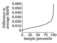
Figure 10: Sorted differences in MAPE between OLS and WLS. Positive values indicate improvements in WLS.

4 Implication of the Model

This paper documented the distribution of $\hat{m}$ and estimated probe counts based on the point probe location data recorded at fixed intervals. The final section discusses the model’s implications regarding theory, applications, and opportunities.

4.1 Model Characteristics

Practitioners can use $\hat{m}$ as an unbiased estimator of probe traffic volumes in any timeframes. The more probes are present, the more closely the distribution of $\hat{m}$ can be approximated by a normal distribution. The estimation precision measured as CV[$\hat{m}$] is inversely proportional to the square root of actual probe volume $m$, roughly proportional to recording interval $t$, and roughly inversely proportional to cordon length $d$ (Equation 18). In other words, the higher the probe volume, the more precise the volume estimates are likely to be, while the degree of marginal improvement decreases as the traffic volume increases. A lower probe speed also tends to result in better precision when other conditions remain the same. In reality, the speed distribution $g(s)$ can change along with $d$ unless $S$ truly follows uniform motion; therefore, the theoretical optimal cordon length $d$ should be considered a suggestion rather than a perfect means of optimisation. Therefore, it is a reasonable strategy to set the longest possible $d$ that fits the road segment that carries a single traffic probe volume when an analyst does not know the probe data recording interval $t$ or the speed distribution $g(s)$.

However, the relationship between $d$ and CV[$\hat{m}$] is not always monotonic. Depending on the recording interval and speed distribution, there is a local optimum cordon length $d$ that maximises the precision of $\hat{m}$ estimation (Figure 8a). Although the authors are unaware of the exact data processing methods used in proprietary traffic volume estimation software, the estimation precision is likely to improve by setting an optimal cordon length $d$ in these products if they inherently rely on probe point data with speed information.

In developing a traffic volume estimation model, calibration among $\hat{m}$ is required to convert the values into traffic volume estimates. Because probes, in reality, are not likely to be distributed homogeneously among road users, this procedure ultimately determines traffic volume estimation accuracy. In this process, modellers can use the theoretical variance to effectively weight $\hat{m}$ (Figure 10).

Knowledge of how the distribution emerges can improve the traffic volume estimation models, as shown in Figure 8. Our method equips modellers with the capability to incorporate even low traffic volumes into their calibration models, as the distribution of $\hat{m}$ cannot always be approximated by a normal distribution when the actual probe volume is low. The theoretical PDF of the estimated probe traffic volume allows modellers or analysts to perform interval estimation on $m$. Depending on the calibration model, probe traffic volume estimates with confidence intervals (CIs) can also be used to improve the calibration accuracy against known traffic volumes.

Practitioners should be aware of some other elements when applying the proposed method to probe point location data. First, spatial characteristics should be considered when drawing virtual cordons. For example, a modeller must pay attention to grade-separated facilities, tunnels, crosswalks, sidewalks, and cell phone location data from flying objects. Sometimes, probe data need to be coded to avoid capturing location data from unintended road users, as we truncated the high speed in our example calculation.

With real traffic, the variance of $\hat{m}$ can become larger than the theoretical variance because GNSS is not free from systematic and random errors (Marković et al., 2019). Although centimetre-level positioning is available with some GNSS (Choy et al., 2015), most GNSS argumentations are associated with horizontal errors varying up to 3-15 meters (Merry and Bettinger, 2019; Zandbergen and Barbeau, 2011). As a result, speed measurement is also associated with some errors (Guido et al., 2014). Because speed distribution plays a crucial role in estimating traffic volumes in the proposed method, it is essential to make an effort to reduce speed bias (Ahsani et al., 2019) in the data acquisition process.

4.1.1 Limitations

Although we addressed the theoretical aspect of traffic volume estimation from probe point data, the proposed model is not free from limitations in practical settings. One limitation is that our model assumes i.i.d. uniform motion as the speed among the probes. As actual traffic conditions may not necessarily suit these assumptions, modellers and analysts should recognise this limitation. With careful selection of cordon locations (both spatially and temporally), biases from these assumptions can be weakened.

In traffic volume estimation, another limitation of the model is that the PDF formulation (Equation 13) of $\hat{m}$ includes the true probe volume $m$ itself. Although this does not prevent the computation of $\hat{m}$ (Equation 1) or VMR[$\hat{m}$] (Equation 17), this recursion is sometimes not ideal, because the probe volume is usually estimated when the probe volume $m$ is unknown. In this context, this study is descriptive and may not be a silver bullet for issues that some readers might have expected to solve. Nevertheless, the theoretical elements of the estimated probe traffic volume still contribute to the lineage of traffic volume estimation research in that we described how the distribution of $\hat{m}$ emerges.

4.2 Applications

The proposed method can contribute to various aspects of traffic volume estimation. First, it allows agencies to use marginal point probe data without pseudonyms or granular timestamps. For example, they can enhance the quality of traffic volume estimation by utilising sparsely recorded probe data, which would have been ignored without our method. Depending on how much marginal probe point data are available compared with the line data already available, probe location data without pseudonyms can be a sleeping lion.

Furthermore, the model predicts “the economy of scale”, encompassing probe data valuation. A higher recording frequency ($\because$ Equation 18) and homogeneity make the traffic volume estimation more precise and accurate, respectively. As a result, probe location data with a high recording frequency and homogeneity are more valuable for traffic volume estimation. Thus, agencies could perform cost-benefit analyses based on the specific goals they want to achieve.

Another economy of scale arises from the synergistic effect of acquiring traffic counts at fixed locations. Probe traffic volumes can be used to estimate traffic volumes at many locations. This fact does not smear the importance of fixed-location traffic counts, because it is impossible to calibrate the values against traffic volumes without ground truths. A higher density of reliable traffic count data from conventional devices can enhance the proposed method by providing additional calibration points. Therefore, governments investing in continuous traffic monitoring infrastructures can expect an even larger return on investment (ROI) than expected.

As reported by Turner (2021), the evaluation of big data quality and valuation has been of concern among transportation professionals, as machine learning models can quickly become black boxes for data users, including decision-makers. In addition to the data availability enhancement, the distribution of $\hat{m}$ can be used to calculate the valuation of probe point data. From Equation 18, it, for example, may be reasonable to formulate the value of point probe data somewhat inversely proportional to the data recording interval $t$.

4.3 Opportunities

The proposed technique can positively impact society, as transportation systems are woven into daily human activities. On a global scale, traffic volume estimations based on probe point data can positively impact agencies and nations with limited financial and human resources (Lord et al., 2003; Yannis et al., 2014). In particular, the method will be useful for low-volume rural roads, where traditional or passive traffic recording tools may not be cost efficient (Das, 2021). Because remote highways tend to have long uninterrupted segments, drawing long virtual cordons would help transportation professionals estimate probe traffic volumes quite precisely. Such traffic volume information along rural highways can be used to develop safety performance functions (SPFs) more thoroughly and continuously than ever before (Tsapakis et al., 2021).

Because traffic volume estimation using probe data is in its infancy, there are many research opportunities in this field. Future research related to traffic volume estimation from probe point data would include the relaxation of the i.i.d. and uniform motion constraints in the distribution of $\hat{m}$, the development of universal indices to describe the homogeneity of probe data, a framework to evaluate the transferability of the data, cost-benefit analyses of probe location data, and real-time crash hotspot identification.

Our model paves the way for unleashing probe point data as a means of social good. In the 1940s, Greenshields (1947) analysed traffic using a series of aerial photographs taken at fixed intervals. Decades later, we have opportunities to improve the quality of transportation through “snapshots” of probes recorded at a fixed interval but with unprecedented scalability. Interorganizational collaborations, including cooperation between the public and private sectors, will be crucial in bringing technology to life to tackle various societal challenges.

Funding Source Declaration

This research was funded in part by the A.P. and Florence Wiley Faculty Fellow provided by the College of Engineering at Texas A&M University.

References

- Ahsani et al. (2019) Ahsani, V., M. Amin-Naseri, S. Knickerbocker, and A. Sharma (2019). Quantitative Analysis of Probe Data Characteristics: Coverage, Speed Bias and Congestion Detection Precision. Journal of Intelligent Transportation Systems 23(2), 103–119. https://doi.org/10.1080/15472450.2018.1502667.
- Alexander et al. (2005) Alexander, S. M., N. M. Waters, and P. C. Paquet (2005). Traffic Volume and Highway Permeability for a Mammalian Community in the Canadian Rocky Mountains. The Canadian Geographer / Le Géographe canadien 49(4), 321–331. https://doi.org/10.1111/j.0008-3658.2005.00099.x.
- Apronti et al. (2016) Apronti, D., K. Ksaibati, K. Gerow, and J. J. Hepner (2016). Estimating Traffic Volume on Wyoming Low Volume Roads Using Linear and Logistic Regression Methods. Journal of Traffic and Transportation Engineering (English Edition) 3(6), 493–506. https://doi.org/10.1016/j.jtte.2016.02.004.
- Barrios and Casburn (2019) Barrios, J. and R. Casburn (2019). Estimating Turning Movement Counts from Probe Data. Technical report, Kittleson & Associates, Inc., Portland, OR. Accessed March 12, 2023, https://www.kittelson.com/wp-content/uploads/2019/11/Estimating-Turning-Movement-Counts-from-Probe-Data_Kittelson.pdf.
- Caceres et al. (2008) Caceres, N., J. Wideberg, and F. G. Benitez (2008). Review of Traffic Data Estimations Extracted from Cellular Networks. IET Intelligent Transport Systems 2(3), 179–192. https://doi.org/10.1049/iet-its:20080003.
- Chang and Cheon (2019) Chang, H.-h. and S.-h. Cheon (2019). The Potential Use of Big Vehicle GPS Data for Estimations of Annual Average Daily Traffic for Unmeasured Road Segments. Transportation 46(3), 1011–1032. https://doi.org/10.1007/s11116-018-9903-6.
- Chen et al. (2019) Chen, P., S. Hu, Q. Shen, H. Lin, and C. Xie (2019). Estimating Traffic Volume for Local Streets with Imbalanced Data. Transportation Research Record 2673(3), 598–610. https://doi.org/10.1177/0361198119833347.
- Choy et al. (2015) Choy, S., K. Harima, Y. Li, M. Choudhury, C. Rizos, Y. Wakabayashi, and S. Kogure (2015). GPS Precise Point Positioning with the Japanese Quasi-Zenith Satellite System LEX Augmentation Corrections. Journal of Navigation 68(4), 769–783. https://doi.org/10.1017/S0373463314000915.
- Codjoe et al. (2020) Codjoe, J., R. Thapa, and A. S. Yeboah (2020, December). Exploring Non-Traditional Methods of Obtaining Vehicle Volumes. Technical Report FHWA/LA.20/635, Louisiana Transportation Research Center, Baton Rouge, LA. https://rosap.ntl.bts.gov/view/dot/58337.
- Das (2021) Das, S. (2021). Traffic Volume Prediction on Low-volume Roadways: A Cubist Approach. Transportation Planning and Technology 44(1), 93–110. https://doi.org/10.1080/03081060.2020.1851452.
- de Montjoye et al. (2013) de Montjoye, Y.-A., C. A. Hidalgo, M. Verleysen, and V. D. Blondel (2013). Unique in the crowd: The privacy bounds of human mobility. Scientific Reports 3(1), 1376. https://doi.org/10.1038/srep01376.
- El-Basyouny and Sayed (2010) El-Basyouny, K. and T. Sayed (2010). Safety Performance Functions with Measurement Errors in Traffic Volume. Safety Science 48(10), 1339–1344. https://doi.org/10.1016/j.ssci.2010.05.005.
- Federal Highway Administration (2016) Federal Highway Administration (2016, April). Federal Register Volume 81, Number 50. https://www.govinfo.gov/content/pkg/FR-2016-03-15/html/2016-05190.htm.
- Fish et al. (2021) Fish, J. K., S. E. Young, A. Wilson, and B. Borlaug (2021, September). Validation of Non-Traditional Approaches to Annual Average Daily Traffic (AADT) Volume Estimation. Technical Report FHWA-PL-21-033, National Renewable Energy Laboratory, Golden, CO. https://rosap.ntl.bts.gov/view/dot/64900.
- Greenshields (1934) Greenshields, B. D. (1934). The Photographic Method of Studying Traffic Behavior. In Proceedings of the Thirteenth Annual Meeting of the Highway Research Board Held at Washington, D.C. December 7-8, 1933. Part I: Reports of Research Committees and Papers, Volume 13, pp. 382–396. Highway Research Board. https://onlinepubs.trb.org/Onlinepubs/hrbproceedings/13/13-026.pdf.
- Greenshields (1947) Greenshields, B. D. (1947). The Potential Use of Aerial Photographs in Traffic Analysis. In Proceedings of the Twenty-Seventh Annual Meeting of the Highway Research Board Held at Washington, D.C. December 2-5, 1947, Washington, D.C., pp. 291–297. Highway Research Board. https://onlinepubs.trb.org/Onlinepubs/hrbproceedings/27/27-028.pdf.
- Guido et al. (2014) Guido, G., V. Gallelli, F. Saccomanno, A. Vitale, D. Rogano, and D. Festa (2014). Treating Uncertainty in the Estimation of Speed from Smartphone Traffic Probes. Transportation Research Part C: Emerging Technologies 47, 100–112. https://doi.org/10.1016/j.trc.2014.07.003.
- Harrison et al. (2020) Harrison, G., S. M. Grant-Muller, and F. C. Hodgson (2020). New and Emerging Data Forms in Transportation Planning and Policy: Opportunities and Challenges for “Track and Trace” Data. Transportation Research Part C: Emerging Technologies 117, 102672. https://doi.org/10.1016/j.trc.2020.102672.
- Jessberger et al. (2016) Jessberger, S., R. Krile, J. Schroeder, F. Todt, and J. Feng (2016). Improved Annual Average Daily Traffic Estimation Processes. Transportation Research Record 2593(1), 103–109. https://doi.org/10.3141/2593-13.
- Krile and Schroeder (2016) Krile, R. and J. Schroeder (2016, February). Assessing Roadway Traffic Count Duration and Frequency Impacts on Annual Average Daily Traffic Estimation: Evaluating Special Event, Recreational Travel, and Holiday Traffic Variability. Technical Report FHWA-PL-16-016, Battelle, Columbus, OH. https://rosap.ntl.bts.gov/view/dot/58038.
- Krile and Slone (2021) Krile, R. and E. Slone (2021, November). Evaluating Two Different Traffic Data Methods Based on Data Observed, Analysis of Provided Data - Final Report A. Technical Report FHWA-PL-021-040, Battelle, Columbus, OH. https://rosap.ntl.bts.gov/view/dot/64901.
- Lord et al. (2003) Lord, D., H. M. Abdou, A. N’Zué, G. Dionne, and C. Laberge-Nadeau (2003). Traffic Safety Diagnostics and Application of Countermeasures for Rural Roads in Burkina Faso. Transportation Research Record 1846(1), 39–43. https://doi.org/10.3141/1846-07.
- Luria et al. (1990) Luria, M., R. Weisinger, and M. Peleg (1990). CO and NOx Levels at the Center of City Roads in Jerusalem. Atmospheric Environment. Part B. Urban Atmosphere 24(1), 93–99. https://doi.org/10.1016/0957-1272(90)90014-L.
- Macfarlane and Copley (2020) Macfarlane, G. S. and M. J. Copley (2020, December). A Synthesis of Passive Third-Party Data Sets Used for Transportation Planning. Technical Report UT-20.20, Brigham Young University, Provo, UT. https://rosap.ntl.bts.gov/view/dot/54890.
- Marković et al. (2019) Marković, N., P. Sekuła, Z. Vander Laan, G. Andrienko, and N. Andrienko (2019). Applications of Trajectory Data From the Perspective of a Road Transportation Agency: Literature Review and Maryland Case Study. IEEE Transactions on Intelligent Transportation Systems 20(5), 1858–1869. https://doi.org/10.1109/TITS.2018.2843298.
- Meng et al. (2017) Meng, C., X. Yi, L. Su, J. Gao, and Y. Zheng (2017). City-Wide Traffic Volume Inference with Loop Detector Data and Taxi Trajectories. In Proceedings of the 25th ACM SIGSPATIAL International Conference on Advances in Geographic Information Systems, SIGSPATIAL ’17, New York, NY. Association for Computing Machinery. https://doi.org/10.1145/3139958.3139984.
- Merry and Bettinger (2019) Merry, K. and P. Bettinger (2019). Smartphone GPS Accuracy Study in an Urban Environment. PLOS ONE 14(7), e0219890. https://doi.org/10.1371/journal.pone.0219890.
- Mitra and Washington (2012) Mitra, S. and S. Washington (2012). On the Significance of Omitted Variables in Intersection Crash Modeling. Accident Analysis & Prevention 49, 439–448. https://doi.org/10.1016/j.aap.2012.03.014.
- Okamoto et al. (1990) Okamoto, S., K. Kobayashi, N. Ono, K. Kitabayashi, and N. Katatani (1990). Comparative Study on Estimation Methods for NOx Emissions from a Roadway. Atmospheric Environment. Part A. General Topics 24(6), 1535–1544. https://doi.org/10.1016/0960-1686(90)90062-R.
- Oppenlander (1963) Oppenlander, J. C. (1963). Sample Size Determination for Spot-Speed Studies at Rural, Intermediate, and Urban Locations. Highway Research Record: Journal of the Highway Research Board (35), 78–80. https://onlinepubs.trb.org/Onlinepubs/hrr/1963/35/35-004.pdf.
- Park et al. (2010) Park, B.-J., Y. Zhang, and D. Lord (2010). Bayesian Mixture Modeling Approach to Account for Heterogeneity in Speed Data. Transportation Research Part B: Methodological 44(5), 662–673. https://doi.org/10.1016/j.trb.2010.02.004.
- Pulugurtha and Mathew (2021) Pulugurtha, S. S. and S. Mathew (2021). Modeling AADT on Local Functionally Classified Roads Using Land Use, Road Density, and Nearest Nonlocal Road Data. Journal of Transport Geography 93, 103071. https://doi.org/10.1016/j.jtrangeo.2021.103071.
- Ritchie (1986) Ritchie, S. G. (1986). Statistical Approach to Statewide Traffic Counting. Transportation Research Record 1090, 14–21. https://onlinepubs.trb.org/Onlinepubs/trr/1986/1090/1090-003.pdf.
- Roll (2019) Roll, J. (2019). Evaluating Streetlight Estimates of Annual Average Daily Traffic in Oregon. Technical Report OR-RD-19-11, Oregon Department of Transportation, Salem, OR. https://www.oregon.gov/odot/Programs/ResearchDocuments/StreetlightEvaluation.pdf.
- Schewel et al. (2021) Schewel, L., S. Co, C. Willoughby, L. Yan, N. Clarke, and J. Wergin (2021, September). Non-Traditional Methods to Obtain Annual Average Daily Traffic (AADT). Technical Report FHWA-PL-21-030, StreetLight Data, San Francisco, CA. https://rosap.ntl.bts.gov/view/dot/64897.
- Seiler and Helldin (2006) Seiler, A. and J. O. Helldin (2006). Mortality in Wildlife Due to Transportation. In J. Davenport and J. L. Davenport (Eds.), The Ecology of Transportation: Managing Mobility for the Environment, pp. 165–189. Dordrecht, Netherlands: Springer Netherlands. https://doi.org/10.1007/1-4020-4504-2_8.
- Sekuła et al. (2018) Sekuła, P., N. Marković, Z. Vander Laan, and K. F. Sadabadi (2018). Estimating Historical Hourly Traffic Volumes via Machine Learning and Vehicle Probe Data: A Maryland Case Study. Transportation Research Part C: Emerging Technologies 97, 147–158. https://doi.org/https://doi.org/10.1016/j.trc.2018.10.012.
- Selby and Kockelman (2013) Selby, B. and K. M. Kockelman (2013). Spatial Prediction of Traffic Levels in Unmeasured Locations: Applications of Universal Kriging and Geographically Weighted Regression. Journal of Transport Geography 29, 24–32. https://doi.org/10.1016/j.jtrangeo.2012.12.009.
- Sfyridis and Agnolucci (2020) Sfyridis, A. and P. Agnolucci (2020). Annual Average Daily Traffic Estimation in England and Wales: An application of Clustering and Regression Modelling. Journal of Transport Geography 83, 102658. https://doi.org/10.1016/j.jtrangeo.2020.102658.
- Sun and Das (2015) Sun, X. and S. Das (2015, July). Developing a Method for Estimating AADT on All Louisiana Roads. Technical Report FHWA/LA.14/548, University of Louisiana at Lafayette, Lafayette, LA. https://rosap.ntl.bts.gov/view/dot/29681.
- Sun et al. (2013) Sun, Z., B. Zan, X. J. Ban, and M. Gruteser (2013). Privacy Protection Method for Fine-grained Urban Traffic Modeling Using Mobile Sensors. Transportation Research Part B: Methodological 56, 50–69. https://doi.org/10.1016/j.trb.2013.07.010.
- Texas Department of Transportation (2022) Texas Department of Transportation (2022, December). TxDOT AADT Annuals. Accessed March 8, 2023, https://gis-txdot.opendata.arcgis.com/datasets/txdot-aadt-annuals/explore.
- Tsapakis et al. (2020) Tsapakis, I., L. Cornejo, and A. Sánchez (2020). Accuracy of Probe-Based Annual Average Daily Traffic (AADT) Estimates in Border Regions. Technical report, Texas A&M Transportation Institute, El Paso, Texas. https://static.tti.tamu.edu/tti.tamu.edu/documents/TTI-2020-1.pdf.
- Tsapakis et al. (2021) Tsapakis, I., S. Das, A. Khodadadi, D. Lord, J. Morris, and E. Li (2021, March). Use of Disruptive Technologies to Support Safety Analysis and Meet New Federal Requirements. Technical report, Texas A&M Transportation Institute, College Station, TX. https://safed.vtti.vt.edu/wp-content/uploads/2021/04/Final-Version-04-113-Use-of-Disruptive-Technologies-to-Support-Safety-Analysis-and-Meet-New-Federal-Requirements.pdf.
- Tsapakis et al. (2021) Tsapakis, I., S. Turner, P. Koeneman, and P. R. Anderson (2021, September). Independent Evaluation of a Probe-Based Method to Estimate Annual Average Daily Traffic Volume. Technical Report FHWA-PL-21-032, Texas A&M Transportation Institute, College Station, TX. https://rosap.ntl.bts.gov/view/dot/64899.
- Turner et al. (2020) Turner, S., I. Tsapakis, and P. Koeneman (2020, November). Evaluation of StreetLight Data’s Traffic Count Estimates From Mobile Device Data. Technical Report MN 2020-30, Texas A&M Transportation Institute, College Station, TX. https://rosap.ntl.bts.gov/view/dot/57948.
- Turner (2021) Turner, S. M. (2021). Making the Most of Big Data and Data Analytics. ITE Journal 91(2), 24–26.
- Yang et al. (2020) Yang, H., M. Cetin, and Q. Ma (2020, March). Guidelines for Using StreetLight Data for Planning Tasks. Technical Report FHWA/VTRC 20-R23, Virginia Transportation Research Council, Charlottesville, VA. https://rosap.ntl.bts.gov/view/dot/55501.
- Yannis et al. (2014) Yannis, G., E. Papadimitriou, and K. Folla (2014). Effect of GDP Changes on Road Traffic Fatalities. Safety Science 63, 42–49. https://doi.org/10.1016/j.ssci.2013.10.017.
- Zandbergen and Barbeau (2011) Zandbergen, P. A. and S. J. Barbeau (2011). Positional Accuracy of Assisted GPS Data from High-sensitivity GPS-enabled Mobile Phones. Journal of Navigation 64(3), 381–399. https://doi.org/10.1017/s0373463311000051.
- Zarei and Hellinga (2022) Zarei, M. and B. Hellinga (2022). Method for Estimating the Monetary Benefit of Improving Annual Average Daily Traffic Accuracy in the Context of Road Safety Network Screening. Transportation Research Record, 03611981221115720. https://doi.org/10.1177/03611981221115720.
- Zhan et al. (2017) Zhan, X., Y. Zheng, X. Yi, and S. V. Ukkusuri (2017). Citywide Traffic Volume Estimation Using Trajectory Data. IEEE Transactions on Knowledge and Data Engineering 29(2), 272–285. https://doi.org/10.1109/TKDE.2016.2621104.
- Zhang and Chen (2020) Zhang, X. and M. Chen (2020). Enhancing Statewide Annual Average Daily Traffic Estimation with Ubiquitous Probe Vehicle Data. Transportation Research Record 2674(9), 649–660. https://doi.org/10.1177/0361198120931100.
- Zhang et al. (2019) Zhang, X., C. V. Dyke, G. Erhardt, and M. Chen (2019). Practices on Acquiring Proprietary Data for Transportation. Washington, D.C.: The National Academies Press. https://doi.org/10.17226/25519.
- Zhao et al. (2019) Zhao, J., H. Xu, H. Liu, J. Wu, Y. Zheng, and D. Wu (2019). Detection and Tracking of Pedestrians and Vehicles Using Roadside LiDAR Sensors. Transportation Research Part C: Emerging Technologies 100, 68–87. https://doi.org/10.1016/j.trc.2019.01.007.
- Zhong and Hanson (2009) Zhong, M. and B. L. Hanson (2009). GIS-based Travel Demand Modeling for Estimating Traffic on Low-class Roads. Transportation Planning and Technology 32(5), 423–439. https://doi.org/10.1080/03081060903257053.