Solving two-dimensional adjoint QCD with a basis-function approach

Uwe Trittmann

Department of Physics
Otterbein University
Westerville, OH 43081, USA

Abstract

We apply a method (“eLCQ”) to find the asymptotic spectrum of a Hamiltonian from its symmetries to two-dimensional adjoint QCD. Streamlining the approach, we construct a complete set of asymptotic eigenfunctions in all parton sectors and use it in a basis-function approach to find the spectrum of the full theory. We are able to reproduce previous results including the degeneracy of fermionic and bosonic masses at the supersymmetric point, and to understand the properties of the lowest states in the massless theory.

The approach taken here is continuous at fixed parton number, and therefore complementary to standard (DLCQ-like) formulations. Despite its limitation to rather small parton numbers, it can be used to test and validate conclusions of other frameworks in an independent way.

1 Introduction

In the last years there has been renewed interest in two-dimensional adjoint quantum chromodynamics (QCD_2A), as new methods and computational resources have become available [1, 2, 3, 4]. The theory has been generalized and thereby become interesting for other subfields [5]. It is simpler in the large $N$ limit, but forays into finite $N$ calculation [6] have recently been put on a solid foundation [4]. The theory of massive adjoint fermions is confining and possesses a supersymmetric point at $m_{adj}=g^{2}N/\pi$ [7]. Its features are well reproduced in numerical studies starting with [8, 9]. The massless theory can be bosonized, i.e. cast into a theory of currents obeying a Kac-Moody algebra [21]. For several reasons it is the more interesting and challenging version of QCD_2A. For instance, pair production is likely important, and thus sectors of different parton number are coupled. Lately, there have been discussions [2, 10, 3] about the conjectured screening-confinement transition [11] as the fermion mass vanishes, $m_{adj}\rightarrow 0$. To extract the true single-particle content of the theory has been difficult because single-particle states cannot be identified with single-trace states [13]. As was shown numerically starting with [14], at least some of the single-trace eigenstates of QCD₂ must be categorized as multi-particle states. This was corroborated in [17] by the fact that in the bosonized theory exact multi-particle states, i.e. states with the same mass as a state of non-interacting partons, are projected out.

To see how the present approach can better our understanding of QCD_2A, it is helpful to review some of the literature on the subject in more detail. For starters, QCD_2A is a 1+1 dimensional SU($N$) gauge theory coupled to a (Majorana) fermion in the adjoint representation. It is a modification of the ’t Hooft model [12], where the SU($N$) gauge fields are coupled to a fundamental Dirac fermion. Using a $1/N$ expansion, ’t Hooft was able to solve the theory in the large $N$ limit, and its spectrum became the first to exhibit confinement: the fermion-antifermion (mesonic) bound states are arranged in a single linear Regge trajectory, i.e. the bound state masses (squared) are proportional to an integer excitation number. The restriction to two dimensions means that the gauge fields (gluons) are not dynamical. Their equations of motion show up as constraint equations on the way to deriving the Hamiltonian of the theory. This is in stark contrast to four-dimensional QCD, so to study the dynamics of adjoint degrees of freedom QCD_2A was devised. Here, the adjoint fermions form bound states analogous to glueballs in higher dimensional pure Yang-Mills theories. Since the adjoints are fermions, sometimes these bound states are called gluinoballs and interpreted as closed string excitations. Since the gluinoballs can contain an arbitrary number of (fermionic) partons, its spectrum is much richer. Two Regge trajectories of bound states are known to exist; from a conjectured Hagedorn transition one expects an exponentially increasing density of states. Furthermore, the two-index fields allow for discrete versions of $\theta$-vacua [21], i.e. non-trivial topological sectors. Numerical work [9, 14, 17] has naturally focused on the massive bound-state spectrum of both the massive and the massless theory, occasionally exploring the ramifications of the massless sector for the massive spectrum [14] , based on the universality of two-dimensional theories [13].

One strand of new results stems from the finding in [14] that there exist multi-particle states built from the true degrees of freedom of the theory, i.e. the single-particle states made of strings of adjoint fermions. The masses of these multi-particle states at a certain harmonic resolution $K$ can often be expressed as sums of masses at lower resolutions, such that $K_{1}+K_{2}=K$ in typical DLCQ relations

$$M^{2}(K)=K\left[\frac{M^{2}(K_{1})}{K_{1}}+\frac{M^{2}(K_{2})}{K_{2}}\right].$$ (1)

However, some such relations are only approximate, and one runs into problems with statistics, e.g. two fermionic single-particle states forming a fermionic multi-particle state, so one has to invoke the massless sector for explanations. Nonetheless, the great advantage of the DLCQ approach with its consistent IR cutoff ($1/K$ plays the role of smallest momentum), is that one generates a faithful representation of the underlying algebraic structure, and can thus use representation theory to classify and relate states. This program has recently reached near completion, when Klebanov et al. extended QCD_2A by including $N_{f}$ fundamental Dirac fermions [3], and considered the theory at finite $N$ [4]. The trove of results and explanations of degeneracies leaves little doubt that the spectrum is well understood qualitatively in the light-cone gauge $A^{+}=0$. In particular, the massless theory ($m_{adj}=0$) can be “deconstructed” on the grounds of the Kac-Moody algebra of its currents and a newfound $osp(1|4)$ symmetry related to four “supercharges” involving all dynamic fermion fields. The authors of [3] find that degeneracies, e.g between bosonic and double-trace states of fermionic gluinoballs and massive fermionic mesons, persist even when the fundamental fermions are made massive, $y_{fund}>0$. Therefore they reason that the below-threshold bound states point to a attraction between the fundamental quarks and antiquarks at short distances, while the existence of a threshold at which a continuum starts means that the attractive force is screened by the adjoint massless fermions.

An argument in [2] corroborated in Ref. [10], based on index theorems (“mod 2 argument”) that both massive and massless $QCD_{2A}$ are strongly confining theories for odd $N$ has recently been shown to apply only to the theory with an additional four-fermion term $[{\rm Tr}(\bar{\Psi}\Psi)]^{2}$. In fact, the augmented model is no longer UV finite but rather has logarithmic flow in the UV [22]. The current consensus seems to be that massless QCD_2A proper (without the additional term) is screening, cf. Ref. [15], where it is argued that the existence of newly found super-selection sectors of the massless theory is evidence for its screening behavior. Also [6, 4] show that the spectrum of QCD_2A is largely insensitive to $N$ (which includes $N=3$), suggesting a screening massless theory at odd $N$.

Another issue is the appearance of vacua. For instance, in [23] the flow of UV operators is mapped for generic two-dimensional field theories, and QCD_2A in particular. It is argued that a subset of UV operators ends up as vacua in the extreme infrared where the theory is describable as a topological field theory, and thus would not show up as massive excitations in a Hamiltonian approach. Due to the (naive) trivial vacuum in light-cone quantization, one has a hard time dealing with multiple vacua in this approach. Most often DLCQ-based work [9, 14, 17, 3, 4] assumes light-cone gauge to be principally sound even in the continuum limit. One might be worried that gauge or fermionic zero-modes, absent in the discretized theory with anti-periodic boundary conditions, will change the spectrum in the continuum limit. In fact, the typical DLCQ (free) multi-particle spectrum, Eq. (1), described above suggests the existence of a discrete vacuum angle analogous to a $\theta$-vacuum. This was worked out by the authors of Ref. [20] for SU(2). Their set of vacuum states would imply copies of the masses of lower-resolution versions of the theory consistent with Eq. (1). If this interpretation is correct, then the spectrum of QCD_2A should look much cleaner in the continuum limit, where artifacts of regularization are absent. Additionally, one can ask how to get rid of the “threshold bound states”, if they are not genuine content of the theory. As shown in [3] from representation theory, these single-trace states are degenerate with multi-trace states of the adjoint theory (gluinoballs), and with multi-string states if fundamental fermions are added and meson (open string) states appear. As mentioned, bosonization projects out only the exact multi-particle states. It is unclear what the role of the approximate multi-particle states is. It could be that any discrete approach fails: these states have to be present at any finite representation of the underlying Kac-Moody algebra, but not necessarily in the continuum limit. The crux is that precisely the regularization makes it possible to have a faithful representation of the algebra in the first place; the continuum limit is the infinite parton limit, regardless of whether fermions or currents are used.

In light of these results, we hope that the present work via a different, basis function approach illuminates the theory in a complementary way. Instead of using the underlying algebraic structure, we tackle the theory via the constraints of the integral equation inherent in its Hamiltonian. We use the asymptotic spectrum of the theory [19] to evaluate the spectrum of the full theory. This allows us to understand the masses of the low-lying spectrum, and the emergence of the multi-particle states in the full theory as described by the asymptotic degrees of freedom. Our work shares the shortcomings of a fermionic theory with its predecessors, namely the appearance of exact multi-particle states. On the other hand, we will establish that discretization per se is no fundamental flaw. While quantitatively we do not completely agree with previous results, we see no evidence that the continuum limit would qualitatively change conclusions about the spectrum. For instance, one might be worried that today’s feasible resolutions of DLCQ approaches, while substantially better than decades ago, are still too modest to tame the divergencies of the theory enough to render results accurate.

The paper is organized as follows. In Section 2 we describe the theory in standard Lagrangian form and highlight the challenges in solving the associated eigenvalue problem. In Sec. 3 we take a look at the asymptotic theory and its relation to the method of exhaustively-symmetrized light-cone quantization (eLCQ) [19]. This leads in Sec. 4 to the construction of a complete set of (asymptotic) eigenfunctions, which agree well with known solutions of the theory. These basis functions are then used in Sec. 5 to solve the full theory. To do so, we have to generalize the procedure to integrate over the Coulomb divergence to be applicable to adjoints. The evaluation of the Hamiltonian matrix elements is quite involved in the basis at hand. Nonetheless, it can be done completely analytically, so that the result for a fixed parton number is free of all singularities and approximations — an important feature of the approach. We therefore describe the calculation in some detail, but do so in the appendix, as the main focus is on the spectrum of the theory, which we display in Sec. 6 and then discuss in Sec. 7 before concluding. We note preemptively, that our work is complementary to other approaches [14, 1]. The hope is to get a clearer picture via a view of the theory from a different angle. While we cast doubt on the accuracy of other approaches and we cannot do much better (outside of the asymptotic regime) because of eLCQ’s severe limitation on parton number, we believe we can show that discretized or compactified approaches are not fundamentally flawed when applied to QCD_2A.

2 Theory Overview

2.1 Lagrangian and Mode Expansion

QCD_2A is a non-abelian Yang-Mills theory in two dimensions coupled to fermions in the adjoint representation. It is based on the Lagrangian

$${\cal L}=Tr[-\frac{1}{4g^{2}}F_{\mu\nu}F^{\mu\nu}+i\bar{\Psi}\gamma_{\mu}D^{\mu}\Psi],$$ (2)

where $\Psi=2^{-1/4}({\psi\atop\chi})$, with $\psi$ and $\chi$ being $N\times N$ matrices. The field strength is $F_{\mu\nu}=\partial_{\mu}A_{\nu}-\partial_{\nu}A_{\mu}+i[A_{\mu},A_{\nu}]$, and the covariant derivative is defined as $D_{\mu}=\partial_{\mu}+i[A_{\mu},\cdot]$. We will use light-cone coordinates $x^{\pm}=(x^{0}\pm x^{1})/\sqrt{2}$, where $x^{+}$ plays the role of a time and work in the light-cone gauge, $A^{+}=0$, as is customary — but see Sec. 1 and Ref. [20]. The theory has been discussed in the literature for a while, so we refer the reader to Refs. [8, 9, 14, 3] for further details.

The dynamics of a system of adjoint fermions interacting via a non-dynamical gluon field in two dimensions are described by the light-cone momentum operator $P^{+}$ and the Hamiltonian operator $P^{-}$. Following the canonical procedure involving the energy-momentum tensor $\Theta^{\pm\pm}$, we express the operators in terms of the dynamic fields, namely the right-moving adjoint fermions $\psi_{ij}$ quantized by imposing anticommutation relations at equal light-cone times

$$\left\{\psi_{ij}(x^{-}),\psi_{kl}(y^{-})\right\}=\frac{1}{2}\,\delta(x^{-}-y^{-})\bigl{(}\delta_{il}\delta_{jk}-{1\over N}\delta_{ij}\delta_{kl}\bigr{)}.$$ (3)

The operators are then

$$P^{+} = \int dx^{-}\Theta^{++}=\frac{i}{2}\int dx^{-}{\rm Tr}\{\psi\partial_{-}\psi\}$$

$$P^{-} = \int dx^{-}\Theta^{+-}=-\frac{1}{2}\int dx^{-}{\rm Tr}\{im^{2}\psi\frac{1}{\partial_{-}}\psi+g^{2}J^{+}\frac{1}{\partial^{2}_{-}}J^{+}\},$$

where we introduced the right-moving components $J^{+}_{ij}=\psi_{ik}\psi_{kj}$ of the SU(N) current. One uses the usual decomposition of the fields in terms of fermion operators

$$\psi_{ij}(x^{-})={1\over 2\sqrt{\pi}}\int_{0}^{\infty}dk^{+}\left(b_{ij}(k^{+}){\rm e}^{-ik^{+}x^{-}}+b_{ji}^{\dagger}(k^{+}){\rm e}^{ik^{+}x^{-}}\right),$$ (4)

with anti-commutation relations following from Eq. (3)

$$\{b_{ij}(k^{+}),b_{lk}^{\dagger}(p^{+})\}=\delta(k^{+}-{p}^{+})(\delta_{il}\delta_{jk}-\frac{1}{N}\delta_{ij}\delta_{kl})\,\,.$$ (5)

The dynamics operators then read

$$P^{+} = \int_{0}^{\infty}dk\ k\,b_{ij}^{\dagger}(k)b_{ij}(k)\ ,$$ (6)

$$P^{-} = {m^{2}\over 2}\,\int_{0}^{\infty}{dk\over k}b_{ij}^{\dagger}(k)b_{ij}(k)+{g^{2}N\over\pi}\int_{0}^{\infty}{dk\over k}\ C(k)b_{ij}^{\dagger}(k)b_{ij}(k)$$

$$+{g^{2}\over 2\pi}\int_{0}^{\infty}dk_{1}dk_{2}dk_{3}dk_{4}\biggl{\{}B(k_{i})\delta(k_{1}+k_{2}+k_{3}-k_{4})$$

$$\qquad\qquad\times(b_{kj}^{\dagger}(k_{4})b_{kl}(k_{1})b_{li}(k_{2})b_{ij}(k_{3})-b_{kj}^{\dagger}(k_{1})b_{jl}^{\dagger}(k_{2})b_{li}^{\dagger}(k_{3})b_{ki}(k_{4}))$$

$$\qquad+A(k_{i})\delta(k_{1}+k_{2}-k_{3}-k_{4})b_{kj}^{\dagger}(k_{3})b_{ji}^{\dagger}(k_{4})b_{kl}(k_{1})b_{li}(k_{2})$$

$$\qquad+\frac{1}{2}D(k_{i})\delta(k_{1}+k_{2}-k_{3}-k_{4})b_{ij}^{\dagger}(k_{3})b_{kl}^{\dagger}(k_{4})b_{il}(k_{1})b_{kj}(k_{2})\biggl{\}},$$

with

$$A(k_{i}) = {1\over(k_{4}-k_{2})^{2}}-{1\over(k_{1}+k_{2})^{2}}\ ,$$ (7)

$$B(k_{i}) = {1\over(k_{2}+k_{3})^{2}}-{1\over(k_{1}+k_{2})^{2}},$$

$$C(k) = \int_{0}^{k}dp\,\,{k\over(p-k)^{2}},$$

$$D(k_{i}) = \frac{1}{(k_{1}-k_{4})^{2}}-\frac{1}{(k_{2}-k_{4})^{2}},$$

where the trace-splitting term $D(k_{i})$ can be omitted at large $N$, and the parton-number violating term is proportional to $B(k_{i})$. The structure of the Hamiltonian $P^{-}$ is

$$P^{-}=P^{-}_{m}+P^{-}_{ren}+P^{-}_{PC,s}+P^{-}_{PC,ns}+P^{-}_{PV}+P^{-}_{finite\,N}.$$ (8)

While the mass term $P^{-}_{m}$ is absent in the massless theory, the associated renormalization operator $P^{-}_{ren}$ needs to be included. Parton-number violating terms, $P^{-}_{PV}$, couple blocks of different parton number. Parton-number conserving interactions $P^{-}_{PC}$ are block diagonal, and may include singular($s$) or non-singular($ns$) functions of the parton momenta. The finite $N$ term $P^{-}_{finite\,N}$ is proportional to $D(k_{i})$. For details see [8, 9, 18].

2.2 The Eigenvalue Problem

To find the spectrum of the general Hamiltonian (8) we solve the eigenvalue problem

$$2\hat{P}^{+}\hat{P}^{-}|\Psi\rangle\equiv\hat{H}_{LC}|\Psi\rangle=M^{2}|\Psi\rangle$$ (9)

where $H_{LC}$ is the so-called light-cone Hamiltonian. This is a daunting task, since its eigenkets $|\Psi\rangle$ will be linear combinations $|\Psi\rangle=\sum_{r}^{\infty}|\Psi_{r}\rangle$ of states of definite (fermion) parton number $r$

$$|\Psi_{r}\rangle=\int_{0}^{\frac{1}{r}}dx_{1}\left(\prod^{r-1}_{j=2}\int^{1-(r-j+1)x_{1}-\sum^{j-1}_{k=2}x_{k}}_{x_{1}}dx_{j}\right)\frac{\psi_{r}(x_{1},x_{2},\ldots,x_{r})}{N^{r/2}}Tr[b(-x_{1})\cdots b(-x_{r})]|0\rangle.$$ (10)

In practice, one transforms the eigenvalue problem, Eq. (9), into an integral equation for the wavefunctions $\psi_{r}(x_{1},x_{2},\ldots,x_{r})$ which distribute momentum between the partons and the total momentum is set to unity by Lorentz invariance. For instance, in the two-parton sector we have the ’t Hooft-like equation

$$\frac{m^{2}\psi_{2}(x)}{x(1-x)}-\frac{2g^{2}N}{\pi}\mathchoice{{\vbox{\hbox{$\textstyle-$}}\kern-4.86108pt}}{{\vbox{\hbox{$\scriptstyle-$}}\kern-3.25pt}}{{\vbox{\hbox{$\scriptscriptstyle-$}}\kern-2.29166pt}}{{\vbox{\hbox{$\scriptscriptstyle-$}}\kern-1.875pt}}\!\int_{0}^{1}\frac{\psi_{2}(y)}{(x-y)^{2}}dy=\frac{\tilde{m}^{2}\psi_{2}(x)}{x(1-x)}+\frac{2g^{2}N}{\pi}\mathchoice{{\vbox{\hbox{$\textstyle-$}}\kern-4.86108pt}}{{\vbox{\hbox{$\scriptstyle-$}}\kern-3.25pt}}{{\vbox{\hbox{$\scriptscriptstyle-$}}\kern-2.29166pt}}{{\vbox{\hbox{$\scriptscriptstyle-$}}\kern-1.875pt}}\!\int_{0}^{1}\frac{\psi_{2}(x)-\psi_{2}(y)}{(x-y)^{2}}dy=M^{2}\psi_{2}(x),$$ (11)

where $\tilde{m}$ is the renormalized fermion mass and $\psi_{2}(x_{1},x_{2})=\psi_{2}(x,1-x)\equiv\psi_{2}(x)$ due to the momentum constraint

$$P^{+}=\sum_{i=1}^{r}x_{i}=1,$$ (12)

which defines the physical Hilbert space, i.e. the hyperplane of the naive Hilbert space $[0,1]^{r}$ on which this constraint is realized.

A good understanding of the integration domain and therefore the Hilbert space will help us to crucially simplify evaluations of matrix elements for the numerical work in Sec. 5. The quantum theory consists of states with certain symmetries, such as cyclic permutations due traced fermionic operators. Since states related by symmetry operations are equivalent, only a small region of the naive Hilbert space is necessary to completely and uniquely describe the dynamics of the physical system. We call such a region a unique Hilbert space cell (uHS). Without loss of generality, we single out the first $r-1$ momenta, i.e. project onto the $(x_{1},x_{2},\ldots,x_{r-1})$ hyperplane. The uHS is then constructed by ordering tuples of momentum fractions $x_{i}$ so that $x_{1}$ is the smallest, $x_{2}$ the second smallest, etc., i.e. parton momenta are monotonically increasing as possible, which leads to $x_{1}\leq 1/r$, and

$${\rm uHS}\doteq\left[0,\frac{1}{r}\right]\times\prod_{j=2}^{r-1}\left[x_{1},1-(r-j+1)x_{1}-\sum_{k=2}^{j-1}x_{k}\right].$$ (13)

In fact, we have already written out the resulting prescription for integral limits in Eq. (10). The upper integral limits, e.g. in the unique Hilbert space cell volume

$${\cal N}_{r}=\int_{0}^{1/r}dx_{1}\left(\prod^{r-1}_{j=2}\int^{1-(r-j+1)x_{1}-\sum^{j-1}_{k=2}x_{k}}_{x_{1}}dx_{j}\right)=\frac{1}{r!}$$ (14)

monotonically decrease. Yet, the last momentum fraction, $x_{r-1}$, will be the largest, since all redundant cyclic permutations will be purged, and the tuple $(0,0,\ldots,0,1-\sum_{j}x_{j})$ is the first to be constructed in Fock-space generating algorithms such as DLCQ. Note that $(1/r,1/r,\ldots,1/r)$ is a unique point, and $x_{1}$ is a special variable with this choice of ordering. Of course, the formalism is symmetric in all $x_{i}$, but it is not practical to formulate the approach such that the symmetry is manifest.

A physical way to think of the integral domain boundaries is as planes of equal momenta, $x_{i}=x_{j}$, where particle identities, i.e. longitudinal momenta, get swapped. For instance, $x_{3}=x_{1}$ implies $x_{2}=1-x_{1}$ for three partons. Pauli exclusion then dictates that wavefunctions be extreme or zero at these boundaries.

3 The Asymptotic Theory and eLCQ

The coupling of parton sectors is due to the parton-number violating interaction $P^{-}_{PV}$, i.e. pair creation. This coupling suggests that we have to solve the problem on all scales. However, things simplify in the large $M^{2}$ limit, since the form of the integral equation allows one to separate the long-range Coulomb interaction from the rest, which apart from pair creation consists of the non-singular (regular) parton-diagonal interactions. The main argument is that for large eigenvalues $M^{2}$ one can neglect the mass term proportional to $m^{2}$ and the behavior of the integral away from the pole at $x=y$. This allows us to push the integration limits to infinity and to replace Eq. (11) with

$$-\frac{2g^{2}N}{\pi}\int_{-\infty}^{\infty}\frac{\phi(y)}{(x-y)^{2}}dy=M^{2}\phi(x),$$

which has sinusoidal eigenfunctions. We renamed the wavefunction to $\phi$ to make it clear that this is an approximation, and will use $\Psi(x)$ and $\psi(x)$ for the full theory. The Coulomb problem itself is intricate for adjoint fermions due to the “connectedness” of operators under the color trace. Fortunately, this Gordian knot is resolvable by an exponential ansatz paired with group theory in the guise of an exhaustive symmetrization. The approach called eLCQ has been brought forth in [19], albeit in a clumsy way, so we’ll review its salient features in a streamlined fashion here. In short, the approach is based the fact that the total momentum can be set to unity by Lorentz invariance plus the following five defining characteristics of QCD_2A:

1. In the asymptotic regime, the simplest solution of the integral equation based on the singular Coulomb interaction (inverse square behavior) is pure phase

   $$\int^{\infty}_{-\infty}\frac{e^{i\pi ny}}{(x-y)^{2}}dy=-|n|\pi^{2}e^{i\pi nx}.$$

   Therefore a reasonable ansatz for the generic solution is

   $$\chi_{\vec{\nu}}(x_{1},\ldots,x_{r})=\prod_{j=1}^{r-1}e^{i\pi n_{j}x_{j}}=e^{i\pi\sum_{j=1}^{r-1}n_{j}x_{j}}\equiv e^{i\pi\vec{\nu}\cdot\vec{x}},$$ (15)

   where the constraint momentum compels us to operate on a $(r-1)$-hyperplane of the naive $r$-dimensional Hilbert space of $r$ parton states, which is signified by the Greek letter. An eigenfunction of the Hamiltonian will then be a sum of such exponential terms, written for now symbolically as

   $$\phi_{\vec{\nu}}(\vec{x})=\phi_{\vec{\nu}}(x_{1},\ldots,x_{r})=\sum_{{\cal G}\vec{\nu}}(-1)^{s(\vec{\nu})}e^{i\pi\vec{\nu}\cdot\vec{x}}=\sum_{{\cal G}\vec{\nu}}(-1)^{s(\vec{\nu})}\chi_{\vec{\nu}},$$

   where the sign of the term is determined via $s(\vec{\nu})$ by group theoretical arguments, and the sum is over all permutations $g\in{\cal G}$ allowed by the symmetries of the theory, see Eq. (20), below.

2. The cyclic structure of the Hamiltonian $\hat{P}^{-}$ results in a mandatory (anti-)symmetrization of its eigenfunctions under

   $${\cal C}:(x_{1},x_{2},\ldots,x_{r})\longrightarrow(x_{2},x_{3},\ldots,x_{r},x_{1}).$$

   In particular,

   $$\phi(x_{1},x_{2},\ldots,x_{r})=(-1)^{(r+1)}\phi(x_{2},x_{3},\ldots,x_{r},x_{1}).$$ (16)

3. The reality of the fermions results in a mandatory (anti-)symmetrization of the eigenfunctions under complex conjugation. One way of achieving this is to “invert” the momenta with

   $${\cal I}:(x_{1},x_{2},\ldots,x_{r})\longrightarrow(1-x_{1},1-x_{2},\ldots,1-x_{r}).$$

4. The vanishing of the massive wavefunctions if one momentum fraction is zero $\phi(0,x_{2},x_{3},\ldots,x_{r})=0$ and the vanishing of the derivative $\frac{\partial\phi}{\partial x_{1}}(0,x_{2},x_{3},\ldots,x_{r})=0$ of the massless wavefunctions results in a mandatory (anti-)symmetrization of the eigenfunctions under the so-called lower-dimensional inversion

   $${\cal S}:(x_{1},\ldots x_{r})\rightarrow(x_{1},1-x_{2}-x_{1},1-x_{3},1-x_{4},\ldots,1-x_{r}-x_{1}).$$ (17)

5. Finally, the symmetry of the Hamiltonian under flipping of color indices

   $${\cal T}:b_{ij}\longrightarrow b_{ji}$$

   can be used to (anti-)symmetrize under

   $${\cal T}:(x_{1},x_{2},\ldots,x_{r})\longrightarrow(x_{r},x_{r-1},\ldots,x_{1}).$$

   Note that one has to distinguish the transformation of the state under ${\cal T}$ (sector identifier $T_{state}$) from the behavior of its wavefunction under momentum reversal (symmetry quantum number $T$). For instance, in the literature [14, 17], the lowest fermionic state with $M^{2}\approx 5.7\frac{g^{2}N}{\pi}$ has been labeled as a ${\cal T}$ even state. While indeed its wavefunction is constant and trivially even under reversal of the momenta, the state does lie in the $T_{state}=-1$ sector of the theory. Sectors are defined by the states’, not the wavefunctions’ symmetry properties.

These five automorphisms of momentum space completely determine the asymptotic eigenfunctions. It is often useful to think of them as operating in excitation number space:

$${\cal C}:(n_{1},n_{2},\ldots,n_{r-1}) \longrightarrow (-1)^{n_{r-1}}(-n_{r-1},n_{1}-n_{r-1},\ldots,n_{r-2}-n_{r-1}),$$ (18)

$${\cal I}:(n_{1},n_{2},\ldots,n_{r-1}) \longrightarrow (-n_{1},-n_{2},\ldots,-n_{r-1}),$$

$${\cal S}:(n_{1},n_{2},\ldots,n_{r-1}) \longrightarrow (n_{1}-n_{2},-n_{2},-n_{3},\ldots,-n_{r-1}),$$

$${\cal T}:(n_{1},n_{2},\ldots,n_{r-1}) \longrightarrow (-1)^{n_{1}}(-n_{1},n_{r-1}-n_{1},n_{r-2}-n_{1},\ldots,n_{2}-n_{1}).$$

One constructs the eigenfunctions by acting with the operators on a generic single-particle momentum state

$$|\vec{x}\rangle=|x_{1},\ldots x_{r}\rangle={\rm Tr}\left\{b^{\dagger}(x_{1})\cdots b^{\dagger}(x_{r})\right\}|0\rangle$$ (19)

or equivalently on the function

$$\chi_{\vec{\nu}}(x_{1},x_{2},\ldots,x_{r})=\langle x_{1},x_{2},\ldots,x_{r}|n_{1},n_{2},\ldots,n_{r-1}\rangle=e^{i\pi\vec{\nu}\cdot\vec{x}},$$

to produce all distinct operators (algebraic words) ${\cal O}_{k}={\cal C}{\cal I}\cdots{\cal S}{\cal T}{\cal C}^{2}\cdots{\cal I}{\cal S},$ where $k$ is an enumerative index. The (complete) set of such operators is called the total symmetrization group

$${\cal G}\equiv\{{\cal O}_{k}\}.$$ (20)

We find that the order of ${\cal G}$ is $2r!$, which is twice the order of the symmetric group $S_{r}$. This makes sense, since we are in essence permuting $r$ objects (the fermion operators) with an additional optional $Z_{2}$ symmetrization with respect to ${\cal T}$. In essence, the exchange of momentum is the same as swapping partons since they are identified by their longitudinal momentum. Even if we are limited to transpositions of adjacent operators, we can still cover the entire symmetric group $S_{r}$, albeit with an algebraic structure that reflects this. It is unclear whether this scheme can be generalized to higher dimensions.

In practice, one uses a computer to construct these states. Note that this has to be done symbolically since we need to decide which operators are distinct, because numerical matching does not suffice. The direct product of inversions, ${\cal I}$, reorientations ${\cal T}$, and cyclic permutations ${\cal C}$ forms a subgroup ${\cal B}$ of order $4r$ of the full group ${\cal G}$ of order $2r!$. This means we can organize the “statelets” $|n_{1},n_{2}\ldots,n_{r-1}\rangle$ as right cosets of ${\cal B}$ in ${\cal G}$ where the operators in ${\cal B}$ act on $\frac{1}{2}(r-1)!-1$ operators collected in the exhaustive set

$${\cal E}=\{{\cal S}_{1},{\cal S}_{2},\ldots,{\cal S}_{(r-1)!/2-1}\}$$

plus the identity. In [19] we tried to classify these ${\cal S}$ operators further, but it suffices to view them as composite operators involving at least one instance of the “fundamental” ${\cal S}$ operator. In particular, ${\cal S}_{1}={\cal S}$. Then the ${\cal S}_{i}$ are algebraic words like ${\cal SICTSC}^{2}$, and for our purposes we only need to know the number of times the letter ${\cal S}$ appears in the word (two in the example) which we refer to as S-ness. The latter determines the sign of the statelet within the eigenstate. Since ${\cal S}$ is a $Z_{2}$ operator with eigenvalues $S=\pm 1$, we get a minus sign only for odd $S$-ness in the $S=-1$ sectors of the theory.

We conclude that the vanishing of the wavefunction whenever $x_{i}=0$ is rather tricky to implement. Indeed, to achieve $\phi(x_{i}=0)=0$ we need to subtract a term $e^{i\pi\vec{\nu}\cdot\vec{x}}$ that is identical to an existing term at $x_{i}=0$ but different otherwise. But this new term then becomes part of the problem: it too needs to be canceled by yet another term, and so on until the possibilities to form distinct terms are exhausted. On the other hand, once the eigenfunctions are constructed reflecting the symmetries and structure of the Hamiltonian, they will automatically respect Pauli exclusion (vanish for $x_{i}=x_{f}$ where necessary) and be (anti-)periodic at the boundaries of the unique Hilbert space.

We now have a blueprint for the states of the theory. In excitation space we may write it as ($|r\rangle=|n_{1},n_{2},\ldots,n_{r-1}\rangle$)

$$|\phi_{\vec{\nu}}\rangle = |\vec{\nu}\rangle={\cal G}|r\rangle=|r\rangle+{\cal C}|r\rangle+{\cal C}^{2}|r\rangle+\ldots$$

$$= |n_{1},n_{2},\ldots,n_{r-1}\rangle+(-1)^{n_{r-1}}|-n_{r-1},n_{1}-n_{r-1},\ldots,n_{r-2}-n_{r-1}\rangle+\ldots.$$

The next step is to fill in integers for the excitation numbers $n_{i}$ and check which combinations lead to viable states. The task to generate these bona fide states is best left to a computer. The results are displayed in Table 1.

$r$ T I S Sector${}^{\rm mass}_{T_{state}}$ Excitation numbers of lowest states Masses ($g^{2}N\pi$) 2 $-+$ $|o\rangle^{0}_{+}$ $(1),(3),(5),(7)$ $2,6,10,14$ $--$ $|e\rangle^{\mu}_{+}$ $(2),(4),(6),(8)$ $4,8,12,16$ 3 $--$ $|ee\rangle^{0}_{+}$ $(4,2),(6,2),(8,2),(8,4)$ $8,12,16,16$ $++$ $|ee\rangle^{0}_{-}$ $(0,0),(2,2),(4,2),(4,0),(6,2)$ $0,4,8,8,12$ $-+$ $|ee\rangle^{\mu}_{+}$ $(6,2),(8,2),(10,4),(10,2)$ $12,16,20,20$ $+-$ $|ee\rangle^{\mu}_{-}$ $(2,0),(4,0),(6,2),(6,0)$ $4,8,12,12$ 4 $+--$ $|oeo\rangle^{0}_{+}$ $(3,2,1),(5,4,3),(5,6,3),(7,6,3)$ $6,10,12,14$ $-++$ $|oeo\rangle^{0}_{-}$ $(1,2,1),(3,2,1),(3,4,3),(3,6,3)$ $4,6,8,10$ $+-+$ $|eee\rangle^{\mu}_{+}$ $(6,6,4),(8,8,6),(8,10,6),(10,10,6),(10,10,8)$ $12,16,20,20,20$ $-+-$ $|eee\rangle^{\mu}_{-}$ $(4,6,4),(6,6,4),(6,8,6),(6,10,6)$ $12,12,16,16$ 5 $+++$ $|eeee\rangle^{0}_{+}$ $(0,0,0,0),(2,2,2,2),(2,4,4,4),(4,4,4,2),(4,4,4,4)$ $0,4,8,8,8$ $---$ $|eeee\rangle^{0}_{-}$ $(4,4,4,2),(4,6,6,6),(4,6,4,2),(6,6,4,2),(4,8,8,8)$ $8,12,12,12,16$ $++-$ $|eeee\rangle^{\mu}_{+}$ $(4,6,6,4),(6,8,8,6),(6,10,10,6),(8,10,10,6)$ $12,16,20,20$ $--+$ $|eeee\rangle^{\mu}_{-}$ $(8,10,10,6),(8,12,10,6)$,(8,14,12,8) $20,24,28$ 6 $-++$ $|oeoeo\rangle^{0}_{+}$ $(1,2,3,2,1),(1,2,3,4,3),(5,4,3,2,1),(3,4,5,4,3)$ $6,8,10,10$ $+--$ $|oeoeo\rangle^{0}_{-}$ $(1,2,3,4,3),(5,4,3,2,1),(3,6,5,4,3),(5,6,5,4,3)$ $8,10,12^{(2)}$ $--+$ $|eeeee\rangle^{\mu}_{+}$ $(6,10,12,10,6),(6,10,12,12,8),(8,12,14,12,8),$ $24^{(2)},28^{(2)},32,36$ $(8,14,14,12,8),(8,14,16,14,8),(8,14,18,14,8)$ $++-$ $|eeeee\rangle^{\mu}_{-}$ $(8,12,12,10,6),(10,12,12,10,6),(8,12,14,14,10),$ $24^{(2)},28^{(3)}$ $(8,14,14,12,8),(12,14,14,12,8)$ 7 $---$ $|eeeeee\rangle^{0}_{+}$ $(2,4,4,4,4,4),(4,6,6,6,4,2),(4,6,8,6,4,2),$ $8,12,16,16$ $(4,6,8,8,8,4)$ $+++$ $|eeeeee\rangle^{0}_{-}$ (0,0,0,0,0,0),(2,2,2,2,2,2),(2,4,4,4,4,2), (2,4,4,4,4,4) $0,4,8,8$ $-+-$ $|eeeeee\rangle^{\mu}_{+}$ $(8,14,16,16,14,10),(8,14,18,18,16,10),$ $32,36^{(3)}$ $(8,14,18,18,16,12),(10,16,18,18,16,12)$ $+-+$ $|eeeeee\rangle^{\mu}_{-}$ $(6,10,12,12,10,6),(8,14,16,16,14,8),$ $24,32,32,36$ $(8,14,16,16,14,10),(8,14,18,18,14,8)$ 8 $+--$ $|oeoeoeo\rangle^{0}_{+}$ $(3,4,5,4,3,2,1),(5,4,5,4,3,2,1),(3,6,5,4,3,2,1)$ $10,12,12$ $-++$ $|oeoeoeo\rangle^{0}_{-}$ $(1,2,3,4,3,2,1),(3,4,5,4,3,2,1),(3,4,5,6,5,4,3)$ $8,10,12$ $+-+$ $|eeeeeee\rangle^{\mu}_{+}$ $(10,16,20,20,18,14,8),(10,18,20,20,18,14,8)$ $40,40$ $-+-$ $|eeeeeee\rangle^{\mu}_{-}$ $(8,14,18,20,18,14,8),(10,16,20,20,18,14,8)$ $40,40$ 9 $+++$ $|eeeeeeee\rangle^{0}_{+}$ $(0)^{8},(2)^{8},(4,4,4,4,4,4,4,4),$ $0,4,8,8,8$ $(4,4,4,4,4,4,4,2),(2,4,4,4,4,4,4,2)$ $---$ $|eeeeeeee\rangle^{0}_{-}$ $(4,4,4,4,4,4,4,2)$ $8$ $++-$ $|eeeeeeee\rangle^{\mu}_{+}$ $(8,14,18,20,18,14,8)$ $50$ $--+$ $|eeeeeeee\rangle^{\mu}_{-}$ $(12,18,20,22,20,18,10)$ $44$

Table 1: The lowest states in the lowest asymptotic parton sectors including their quantum numbers $TIS$. The sectors are labeled with a subscript indicating behavior under ${\cal T}$ (_±), i.e. $T_{state}=\pm 1$, and superscripts signifying massless (⁰) and massive fermions (^μ).

3.1 Grand Bulk Equivalence and Orthonormality

In light of the symmetries the structure of the Hilbert space becomes clear. Namely, in a unique Hilbert space cell one Fock state ${\rm Tr}\{b(-x_{1})\cdots b(-x_{r})\}|0\rangle$ with a specific tuple of momentum fractions represents $2r!$ such states located in $r!$ different cells of the physical Hilbert space, which is thus tessellated. As a consequence eigenfunctions that are orthogonal on a unique Hilbert space cell will be orthogonal everywhere. The $r!$ unique Hilbert space cells of the physical hyperplane are connected by the four automorphisms ${\cal C}$, ${\cal T}$, ${\cal I}$, and ${\cal S}$ that generate the group ${\cal G}\equiv\langle{\cal C},{\cal T},{\cal I},{\cal S}\rangle$.

Now, the symmetrization of the wavefunctions under $\cal G$ is equivalent to putting a representative of each cell into the linear combination in one specific cell. Mathematically, it is the simple fact that $({g}\nu)\cdot\vec{x}=\nu\cdot({g}\vec{x})$ up to a sign for ${g}\in{\cal G}$. For instance, at $r=4$ we have with ${g}={\cal C}$

$$(-n_{3},n_{1}-n_{3},n_{2}-n_{3})\cdot(x_{1},x_{2},x_{3})=(n_{1},n_{2},n_{3})\cdot(x_{2},x_{3},x_{4}),$$

with $x_{4}=1-x_{1}-x_{2}-x_{3}$ on the physical hyperplane. In other words, a term $e^{i\pi\vec{\nu}\cdot({g}\vec{x})}$ in the Hilbert cell ${g}|\vec{x}\rangle$ is substituting for the term $e^{i\pi({g}\vec{\nu})\cdot\vec{x}}$ in the original cell. Note that the former has the original excitation numbers. Therefore, integrating a $2r!$ term eigenfunction over one unique cell is equivalent to integrating a one-term function over the entire physical Hilbert space (pHS) projected onto the $(x_{1},\ldots,x_{r-1})$ hyperplane. We might call this grand bulk equivalence (GBE), since it holds anywhere in the bulk of the Hilbert space. In lieu of a proof, consider that the integral over the second term (first cyclic permutation, $g={\cal C}$) of the three-parton asymptotic wavefunction is shifted by a change of variables $x_{1}^{\prime}=x_{2},x^{\prime}_{2}=1-x_{1}-x_{2}$ with Jacobian $\frac{\partial(x_{1},x_{2})}{\partial(x_{1}^{\prime},x_{2}^{\prime})}=1$, while its integral domain $uHS_{2}={\cal C}(uHS_{1})$ is the cyclically permuted version of the original. To wit

$$\int_{uHS_{1}}\!\!\!\!d^{2}\vec{x}\,\,e^{i\pi((n_{1}-n_{2})x_{1}-n_{1}x_{2})} = \int_{0}^{1/3}\!\!\!\!dx_{1}\int_{x_{1}}^{1-2x_{1}}\!\!\!\!dx_{2}\,\,e^{i\pi((n_{1}-n_{2})x_{1}-n_{1}x_{2})}$$

$$= \int_{0}^{1/3}\!\!\!\!dx^{\prime}_{2}\int_{x^{\prime}_{2}}^{1-2x^{\prime}_{2}}\!\!\!\!dx^{\prime}_{1}\,\,e^{i\pi(n_{1}x^{\prime}_{1}-n_{2}x^{\prime}_{2})}=\int_{uHS_{2}}\!\!\!\!d^{2}\vec{x}\,\,e^{i\pi(n_{1}x_{1}+n_{2}x_{2})},$$

where we omitted the primes of the integration variables in the last step. Similar transformations for the other $g\in{\cal G}$ lead to a full coverage of the semi-naive Hilbert space $snHS=\cup_{j=1}^{r!}uHS_{j}$. There are two caveats. Firstly, this only works if we integrate; the wavefunctions themselves are, of course, not the same. Secondly, the $2r!$ terms of an eigenfunction enter with different signs owing to the quantum numbers of the symmetry sector. Since we are mostly interested in evaluating scalar products between two wavefunctions of the same sector, this is of no consequence as we are squaring the sign.

If exploiting GBE seems too good to be true, note firstly that it is simply a consequence of the structure of the Hamiltonian. For instance, the much simpler ’t Hooft Hamiltonian leads to fewer constraints, hence larger (and fewer) Hilbert space cells, and therefore to the same result: integration of a single sinusoidal function over the entire semi-naive Hilbert space suffices. Secondly, GBE is of little practical use unless the function integrand is invariant under ${\cal G}$. Unfortunately, this is not the case for the Hamiltonian matrix elements as they depend on specific momenta on the physical hyperplane of the naive Hilbert space. If nothing else, GBE allows for an effortless proof of the orthonormality of the asymptotic eigenfunctions

$$\langle\vec{\mu}|{\vec{\nu}}\rangle=\int_{uHS}\!\!\!\!\!\!d^{r-1}\vec{x}\,\,\phi^{*}_{\vec{\mu}}(\vec{x})\phi_{\vec{\nu}}(\vec{x})=\!\!\int_{pHS}\!\!\!\!d^{r-1}\vec{x}\,\,\chi^{*}_{\vec{\mu}}(\vec{x})\chi_{\vec{\nu}}(\vec{x})=\prod_{j=1}^{r-1}\int^{1}_{0}\!\!d{x_{j}}\,\,e^{-i\pi\vec{\mu}\cdot\vec{x}}e^{i\pi\vec{\nu}\cdot\vec{x}}=\delta_{\vec{\mu}\vec{\nu}}.$$

Note that $\langle\vec{\mu}|{\vec{\nu}}\rangle=0$ only implies independent states when $|{\vec{\nu}}\rangle$ and $|{\vec{\mu}}\rangle$ are in different equivalence classes defined by $|{\vec{\nu}}\rangle\approx|{\vec{\mu}}\rangle$ if $|{\vec{\nu}}\rangle=g|{\vec{\mu}}\rangle$ for at least one $g\in{\cal G}$. The Hilbert space is tessellated by $r!$ unique cells, while there are $2r!$ exponential terms or $r!$ statelets representing trigonometric functions. The normalization factor is

$${\cal N}=\sqrt{\frac{r!{\cal N}_{0}}{\mbox{\#statelets}}},$$ (22)

where for almost all eigenfunctions ${\cal N}_{0}=2$ save for the constant $\vec{\nu}=\vec{0}$ functions (appearing in the odd parton $T_{state}=(-1)^{(r-1)/2}$ sectors) we have ${\cal N}_{0}=1$. The number of statelets varies due to “accidental” symmetries of excitation number tuplets, see Eq. (1) and similar.

4 Constructing an Asymptotic Eigenfunction Basis

In the previous section we presented the principles of finding a set of harmonic eigensolutions for asymptotic QCD_2A and listed the resulting bona fide states separately for the lowest parton sectors in all viable symmetry sectors in Table 1. We will now see that the approach can be applied to construct the complete (asymptotic) spectrum of $QCD_{2A}$. The hope is that it can be generalized to tackle other theories, too.

4.1 Generic Algorithm based on Ground States

Using Table 1, it is not hard to come up with general, all-parton-sector expressions for the “ground states” of all symmetry and parton sectors, including their masses and symmetry factors. As can be gleaned from Table 1, the expressions will differ substantially for even and odd parton number as well as even and odd excitation numbers. We therefore need to consider eight different cases (fermionic vs. bosonic, massless vs. massive, and $T=\pm$). Masses $\bar{M}^{2}$ are in units $gN^{2}\pi$ (as in Table 1); for instance $\bar{M}^{2}=4\rightarrow M^{2}\approx 39.48\frac{g^{2}N}{\pi}$ in the usual units.

1. The fermionic massless $T=+1$ sector is the easiest to figure out. These are $T_{state}=(-1)^{(r-1)/2}$ states and all symmetry quantum numbers are positive since the lowest state has $r!$ identical statelets which all have to enter with the same sign lest the state vanishes identically. It is easy to read off the lowest five states

   $$|1\rangle^{0}_{f(+)}=|\bar{M}^{2}=0;0^{r-1}\rangle\frac{1}{\sqrt{2r!}}, \!\!\!\!\!\!|2\rangle^{0}_{f(+)}=|\bar{M}^{2}=4;2^{r-1}\rangle\frac{1}{\sqrt{2(r-2)!}},$$

   $$|3\rangle^{0}_{f(+)}=|\bar{M}^{2}=8;4^{r-1}\rangle\frac{1}{\sqrt{2(r-2)!}}, \!\!\!\!\!\!|4\rangle^{0}_{f(+)}=|\bar{M}^{2}=8;4^{r-2},2\rangle\frac{1}{\sqrt{2(r-3)!}},$$

   $$|5\rangle^{0}_{f(+)}=|\bar{M}^{2}=8;2,4^{r-3},2\rangle\frac{1}{\sqrt{8(r-4)!}},$$ (23)

   where we displayed the symmetry factor of the states under the square root. For instance, the ground state has $2r!$ identical statelets in which all $r-1$ excitation numbers are zero $|0,0,\ldots,0\rangle$. Note that the masses do not depend on the parton number $r$, and thus we expect high-parton-number sectors to contribute significantly if parton number violation is allowed.

2. The massless fermionic $T=-1$ sector has $T_{state}=(-1)^{(r+1)/2}$ states which have asymmetric excitation number tuples. The symmetry quantum numbers are opposite of the previous sector, so $TIS=(---)$

   $$|1\rangle^{0}_{f(-)}=|\bar{M}^{2}=8;4^{(r-2)},2\rangle\frac{1}{\sqrt{2(r-3)!}}.$$

3. The massive fermionic $T=+1$ sector with $T_{state}=(-1)^{(r-1)/2}$ states can be symmetric in excitation numbers (the ground state is!). The symmetry quantum numbers are $TIS=(+,(-)^{\frac{r-1}{2}},(-)^{\frac{r+1}{2}})$ and the lowest state is

   $$|1\rangle^{\mu}_{f(+)}=|\bar{M}^{2}=2\sum^{r}_{even\,j}r-j;r-1,2(r-2),3(r-3),\ldots,2(r-2),r-1\rangle/\sqrt{2}.$$

4. The massive fermionic $T=-1$ sector with $T_{state}=(-1)^{(r+1)/2}$ states. There is no symmetry here; all symmetry factors are one, $TIS=(-,(-)^{\frac{r+1}{2}},(-)^{\frac{r-1}{2}})$

   $$|1\rangle^{\mu}_{f(-)}=|\bar{M}^{2}=6r-10;r+3,2r,2(r+1),2(r+2),\ldots 2(r+2),2(r+1),2r,r+1\rangle.$$

   Mass squared is $\bar{M}^{2}=12$ for $r=3$ and $\bar{M}^{2}=6r-10$ otherwise, so growing linearly with parton number $r$.

5. The massless bosonic $T=+1$ sector with $T_{state}=(-1)^{r/2}$ states are

   $$|1\rangle^{0}_{b(+)}=|\bar{M}^{2}=r+2;3,4,5,\ldots\frac{r}{2}-1,\frac{r}{2},\frac{r}{2}-1,\ldots,2,1\rangle/\sqrt{(r/2+1)!}.$$

   The mass grows linearly with parton number.

6. The massless bosonic $T=-1$ sector with $T_{state}=(-1)^{r/2-1}$, states having symmetric excitation number tuples

   $$|1\rangle^{0}_{b(-)}=|\bar{M}^{2}=\bar{r};1,2,3,\ldots\frac{r}{2}-1,\frac{r}{2},\frac{r}{2}-1,\ldots,2,1\rangle\frac{1}{\sqrt{2\prod^{r/2}_{j=2}j^{2}}},$$

   with $\bar{r}=r$ for $r>2$ and one for $r=2$. Note that mass is proportional to $r$, so high parton-number states should not contribute much to the lowest states of the full theory. Note also that due to the large symmetry factor there are only $2r!/2\prod^{r/2}_{j=2}j^{2}=6,20,70,\ldots$ independent statelets for $r=4,6,8,\ldots$. This is an example for an “accidental” symmetry we alluded to in [19].

7. The massive bosonic $T=+1$ sector with $T_{state}=(-1)^{r/2}$ states with no symmetries (factors all one). The lowest state is

   $$|1\rangle^{\mu}_{b(+)}=|\bar{M}^{2}=r\left(\frac{r}{2}+1\right);r+2,2r,3r-2,\ldots,R,R,\ldots,3(r-2),2(r-1),r\rangle,$$

   with $R:=\frac{r}{2}\left(\frac{r}{2}+1\right)$.

8. The massive bosonic $T=-1$ sector with $T_{state}=(-1)^{r/2-1}$ states. A subset of them was constructed in [7]. A symmetric representative of the ground state is

   $$|1\rangle^{\mu}_{b(-)}=|\bar{M}^{2}=2\sum^{r}_{even\,j}j;r,2(r-1),3(r-2),4(r-3),\ldots,R,\ldots,3(r-2),2(r-1),r\rangle/\sqrt{2}.$$

   Note that the mass increases with the parton number, and that a simpler representative of the state is

   $$|1^{\prime}\rangle^{\mu}_{b(-)}=|\bar{M}^{2}=2\sum^{r}_{even\,j}j;r,0,r-2,0,r-4,0,\ldots,0,2\rangle/\sqrt{2}.$$

   Since every other excitation number is zero in this statelet, it looks like the state can be characterized by $r/2$ excitation numbers, see Sec. 4.3. The symmetry factor suggests that this is not the most general state of the sector.

Now that the ground states are known, we can construct the rest of the spectrum by acting with the “ladder operators”

$$\hat{\cal L}_{i}:|n_{1},n_{2},\ldots,n_{i},\ldots,n_{r-1}\rangle\longrightarrow|n_{1},n_{2},\ldots,n_{i}+2,\ldots,n_{r-1}\rangle,$$

This will take us from the “highest weight” statelet of a bona fide state to some statelet of a different bona fide state — unless the latter does not exist in the symmetry sector considered, in which case we act with ${\cal L}_{i+1}$, until a desired number of bona fide states is produced.

The astonishing fact that for every parton number only four of eight TIS symmetry sectors give rise to states regardless of whether only even or even and odd excitation numbers are allowed is — of course — due to group theory.

4.2 Extracting the Physics

These combinatorics exercises entail some physics. We saw that massless states likely have significant contributions from all higher parton sectors. Additionally, a look at the $I$ quantum number reveals that in the massless sectors, the $r$ and $r+2$ sectors sport opposite trigonometric functions (sines vs. cosines), whereas in the massive sectors, the trigonometric functions are the same. This holds in both the bosonic and fermionic sectors and will dramatically change the importance of the parton-number violating interaction in the massless versus massive sectors, see Sec. 5.

Note that the wavefunctions are necessarily even(odd) under cyclic rotations of their momenta in the odd(even) parton sectors. The question is then whether they are even or odd under momentum order reversal. For states with three fermionic operators, asymmetric states

$${\cal T}|a\rangle=|b\rangle;\quad|a\rangle\neq|b\rangle$$ (24)

are combined with(out) a relative sign to form ${\cal T}$-even(odd) states $\sqrt{2}|T\pm\rangle=|a\rangle\pm|b\rangle$. Therefore we need a ${\cal T}$-even wavefunction to consistently distribute the momenta. The scheme reverses at $r+2$, where the additional operators yield an extra sign when putting flipped indices in order. Therefore the five-fermion states in the same $T_{state}$ sector have asymmetric states under momentum reversal, and hence a relative sign in Eq. (24). Hence, a $\cal T$-even wavefunction is necessary. Only the symmetric wavefunctions produce massless states, so surprisingly a generic all-sector wavefunction of the full theory will have opposite $\cal T$-symmetry of the wavefunctions in adjacent parton sectors. So it will, for instance, comprise a massless asymptotic state in the $4s-1$ parton sectors, but asymptotic states with rather high mass ($\bar{M}^{2}=8$) in the $4s+1$ sectors ($s=1,2,3,\ldots$). This leads to a large mass gap between the lowest states in a sector, explaining the purity in parton number [8, 9] and the fact that almost any brutalization of the theory leads to the correct mass of the ground state(s).

In fact, much of the insight into the lowest states could have been gleaned from earlier work, e.g. [9, 14, 17], and becomes almost trivial in the eLCQ approach. For instance, the fact that the lowest fermionic and bosonic states are isolated in mass and pure in parton number is a result of the asymptotic spectrum having massless states only in the fermionic sectors. In particular, the lowest state of the full theory is a three-parton fermion and not a two-parton boson since the lowest bosonic state has a mass (squared) of about $\bar{M}^{2}=1$ (${M}^{2}\approx 10\frac{g^{2}N}{\pi}$) whereas the lowest asymptotic fermionic state in the adjoint theory is massless, and acquires a mass (squared) of about $r(r-1)\frac{g^{2}N}{\pi}\approx 5.7\frac{g^{2}N}{\pi}$ via the non-singular parton-number preserving interaction, see Appx. B.3.

In eLCQ it is easy to see that the lowest states are isolated, since the higher-parton states start at quite high mass, see Fig. 2. In particular, the lowest four- and five-parton states are $M^{2}\approx 36\frac{g^{2}N}{\pi}$ and $M^{2}\approx 55\frac{g^{2}N}{\pi}$, so about three- and ten times the ground state mass. Also the surprising find [8] that the lowest $T_{state}+$ state is a very pure five-parton state is clear in eLCQ: the lowest three-parton asymptotic state is at $M^{2}\approx 50\frac{g^{2}N}{\pi}$, since the lowest available excitation numbers in that sector ($TI=--$) are $(4,2)$, implying a large mass. But that’s where it stops: the lowest six- and seven-parton states have a similar mass as their lower-parton counterparts, and therefore none of the higher states are pure in parton number. Incidentally, in Ref. [9] it was speculated that this isolation and purity of the lowest states could be related to the surprising success of the valence quark model in full four-dimensional QCD. We can also answer the question as to why the lowest mass grows linearly with the number of flavors [16]. The terms in the Hamiltonian, Eq. (26) of [17], are at most linear in $N_{f}$, and thus in the absence of eigenvalue repulsion due to isolation, the trajectory $M^{2}_{low}(N_{f})$ is necessary linear, see Fig. 5(b) of [17].

4.3 Comparison to Known Solutions

As a cross-check we compare the eLCQ eigensolutions with the output of other approaches. Two-, four-, and six-parton wavefunctions for one of the two bosonic ${\cal T}$ sectors were presented in Ref. [7], Eqns. (4.12), (4.13) and (4.15). The solutions in [7] are orthogonal and vanish at $x_{i}=0$, so they should be a subset of the massive solutions presented in the present note. Indeed, the lowest states $\phi^{[7]}_{4}(4,2)$ and $\phi^{[7]}_{6}(6,4,2)$ are identical with the eLCQ solutions $\varphi_{4-}(4,0,2)$ and $\varphi_{6+}(6,0,4,0,2)$ including the masses. At $r=4$ the equivalency is $\phi_{4}^{[7]}(n_{1},n_{2})=\varphi_{4-}^{eLCQ}(n_{1},0,n_{2})$. However, we find that some eLCQ states (which are numerically virtually identical with DLCQ results [19]) are not reproduced. This means that the set of states described by [7], Eq. (4.13), is not complete.

In the six parton sector the situation is more complicated. While some states of [7], Eq. (4.15), coincide with eLCQ states, others do not match. Since the former are orthogonal and vanish at the boundary, they must violate some “internal” boundary condition, i.e. a zero or extremal wavefunction on hyperplanes where momentum fractions match, $x_{i}=x_{j}$. Crossing such hyperplanes one enters a different, redundant part of the Hilbert space.

Needless to say, the eLCQ eigenfunctions pass a numerical orthonormality check. Note that the first four $r=4$ eigenvalues are pairwise degenerate, and yet their wavefunctions are orthogonal. Hence, it looks like we have all relevant symmetries taken care of.

5 Solving the theory with a basis-function approach

Now that we have a basis of asymptotic eigenstates $\{|\phi_{\vec{\mu}}\rangle\}$, we use it to solve the full theory. We expand the true eigenstates as linear combinations of asymptotic eigenstates by diagonalizing the Hamiltonian in this asymptotic basis, i.e. by solving the eigenvalue problem ($\hat{H}:=2\hat{P}^{+}\hat{P}^{-}$), cf. Eq. (9)

$$\langle\phi_{\vec{\mu}}|\hat{H}_{full}|\phi_{\vec{\nu}}\rangle=M^{2}\langle\phi_{\vec{\mu}}|\phi_{\vec{\nu}}\rangle.$$ (25)

This is a finite matrix equation when the number of basis states is cut off at $N_{\phi}<\infty$. Convergence is typically exponential in the number of basis states used. Recall that the parton sectors are coupled by the pair-production interaction, so it will be convenient to limit the number of states separately in each parton sector so that $\sum_{r}N_{\phi,r}=N_{\phi}$.

To compute the matrix elements in the asymptotic basis, we need the Hamiltonian in a basis of single-particle momentum eigenstates $\{|\vec{x}\rangle\}$, Eq. (19), where fermionic operators act on a conventional vacuum state. We can easily compute the matrix elements in such a momentum base from the mode expansions, Eq. (6). The relevant operators are the contractions $\hat{P}^{-}_{ren}$ and the singular (Coulomb) part of the parton-conserving interaction $\hat{P^{-}_{PC,s}}$

$$\langle\vec{x}|\hat{H}^{-}_{ren}|\vec{y}\,\rangle = 2\sum_{j=1}^{r=r^{\prime}}\int_{0}^{y_{j}}\frac{dp}{(y_{j}-p)^{2}}\delta(\vec{x}-\vec{y})=2\sum_{j=1}^{r=r^{\prime}}\int_{0}^{x_{j}}\frac{dp}{(x_{j}-p)^{2}}\delta(\vec{x}-\vec{y}),$$

$$\langle\vec{x}|\hat{H}^{-}_{PC}|\vec{y}\,\rangle = \sum_{i=1}^{r^{\prime}}\sum_{j=1}^{r}(-1)^{(r+1)(i+j-2)}\left(\frac{1}{(x_{i}+x_{i+1})(y_{j}+y_{j+1})}-\frac{1}{(x_{i}-y_{j})^{2}}\right)$$

$$\qquad\qquad\times\delta(x_{i}+x_{i+1}-y_{j}-y_{j+1})\delta(\vec{x}_{i,Sp}-\vec{y}_{j,Sp}),$$

$$\langle\vec{x},r^{\prime}|\hat{H}^{-}_{PV}|\vec{y},r\rangle = -\sum_{i=1}^{r^{\prime}}\sum_{j=1}^{r}\delta(\vec{y}_{j,{Sp}}-\vec{x}_{i,{Sp}})$$

$$\times\left[\left(\frac{1}{(y_{j+2}+y_{j+1})^{2}}-\frac{1}{(y_{j}+y_{j+1})^{2}}\right)\delta^{r}_{r^{\prime}+2}\delta(y_{j}+y_{j+1}+y_{j+2}-{x_{i}})\right.$$

$$\quad\,\left.\left(\frac{1}{(x_{i+2}+x_{i+1})^{2}}-\frac{1}{(x_{i}+x_{i+1})^{2}}\right)\delta^{r+2}_{r^{\prime}}\delta(x_{i}+x_{i+1}+x_{i+2}-{y_{j}})\right],$$

where $x_{Sp},y_{Sp}$ are spectator momenta. The matrix elements do not contain a summation over in- or outgoing momenta. This summation/integration appearing in the integral equation is a consequence of the action of the Hamiltonian on the states $|\Phi\rangle$, leading to the appearance of the wavefunctions $\phi(\vec{k})=\langle\vec{k}|\Phi\rangle$. Note that the non-singular term is written manifestly symmetric in in- and outgoing momenta. Then

$$\langle\phi_{\vec{\mu}}|\hat{H}_{full}|\phi_{\vec{\nu}}\rangle=\int_{uHS}\!\!d\vec{x}\int_{uHS}\!\!d\vec{y}\,\,\,\langle\phi_{\vec{\mu}}|\vec{x}\rangle\langle\vec{x}|\hat{H}_{full}|\vec{y}\rangle\langle\vec{y}|\phi_{\vec{\nu}}\rangle,$$ (26)

where we conventionally integrate over “the” Hilbert space, i.e. one unique Hilbert space cell each. Owing to the symmetry structure of the theory, we can do better here in view of ensuing numerical effort if we rewrite this integral. Paradoxically, we do better if we enlarge the domain, because we can subsume the cyclic permutations. In the end, we will be able to write the eigenvalue problem of the adjoint theory in the same form as the fundamental problem [12]. Incidentally, ‘t Hooft used the “trick” of writing the Hamiltonian as a scalar product to show that it is hermitian, not to tame the singularity; the latter is of importance to us.

To proceed it is salutary to distinguish the Hamiltonian matrix element proportional to

$$\sum_{ij}\frac{\delta(x_{i}+x_{i+1}-y_{j}-y_{j+1})\delta(\vec{x}_{rest,i}-\vec{y}_{rest,j})}{(x_{i}-y_{j})^{2}}$$

from the wavefunction part

$$[\phi(\vec{x})-\phi(\vec{y})]_{\mu\nu}:=\frac{1}{2}[\phi_{\mu}(\vec{x})-\phi_{\mu}(\vec{y})][\phi_{\nu}(\vec{x})-\phi_{\nu}(\vec{y})],$$ (27)

which does not carry $i,j$ indices, i.e. is not part of the cyclic permutations. Confusingly, the eigenfunctions themselves are sums over all permutations $g\in{\cal G}$ and are affected by the delta-function variable substitutions. The point is that the enlarging of the integral domain affects only the matrix elements, not the wavefunctions. To wit

$$\!\!\!\!\!\!\!\!\int_{uHS}\!\!\!\!d\vec{x}\int_{uHS}\!\!\!\!d\vec{y}\sum_{ij}\frac{[\phi(\vec{x})-\phi(\vec{y})]_{\mu\nu}}{(x_{i}-y_{j})^{2}}\Delta_{ij}=\int_{uHS}\!\!\!\!d\vec{x}\int_{uHS}\!\!\!\!d\vec{y}\frac{[\phi(\vec{x})-\phi(\vec{y})]_{\mu\nu}}{(x_{1}-y_{1})^{2}}\Delta_{11}$$

$$\!\!\!\!\!\!\!\!+\int_{uHS}\!\!\!\!d\vec{x}\int_{uHS}\!\!\!\!d\vec{y}\frac{[\phi(\vec{x})-\phi(\vec{y})]_{\mu\nu}}{(x_{1}-y_{2})^{2}}\Delta_{12}+\int_{uHS}\!\!\!\!d\vec{x}\int_{uHS}\!\!\!\!d\vec{y}\frac{[\phi(\vec{x})-\phi(\vec{y})]_{\mu\nu}}{(x_{1}-y_{3})^{2}}\Delta_{13}+\ldots$$

$$\!\!\!\!\!\!\!\!=\int_{uHS}\!\!\!\!d\vec{x}\int_{uHS}\!\!\!\!d\vec{y}\frac{[\phi(\vec{x})-\phi(\vec{y})]_{\mu\nu}}{(x_{1}-y_{1})^{2}}\Delta_{11}+\int_{uHS}\!\!\!\!d\vec{x}\int_{{\cal C}uHS}\left|\frac{\partial\vec{y}}{\partial\vec{y}^{\,{}^{\prime}}}\right|d\vec{y}^{\,{}^{\prime}}\frac{[\phi(\vec{x})-\phi(\vec{y}^{\,{}^{\prime}})]_{\mu\nu}}{(x_{1}-{y}^{{}^{\prime}}_{2})^{2}}\Delta^{\prime}_{12}+\ldots$$

$$\!\!\!\!\!\!\!\!=\int_{cHS}\!\!\!\!d\vec{x}\int_{cHS}\!\!\!\!d\vec{y}\,\,\frac{[\phi(\vec{x})-\phi(\vec{y})]_{\mu\nu}}{(x_{1}-y_{1})^{2}}\Delta_{11},$$

where we have defined

$$\Delta_{ij} := \delta(x_{i}+x_{i+1}-y_{j}-y_{j+1})\delta(\vec{x}_{rest,i}-\vec{y}_{rest,j}),$$

$$\Delta^{\prime}_{ij} := \delta(x_{i}+x_{i+1}-y^{\prime}_{j}-y^{\prime}_{j+1})\delta(\vec{x}_{rest,i}-\vec{y}^{\,{}^{\prime}}_{rest,j}),$$

and the union of all unique Hilbert space cells connected to the first one ($x_{1}\leq x_{i}\,\,\forall i\neq 1$) by one of the $r-1$ cyclic permutations

$$\mbox{cHS}:=\mbox{uHS}\cup{\cal C}\mbox{(uHS)}\cup{\cal C}^{2}\mbox{(uHS)}+\ldots\cup{\cal C}^{r-1}\mbox{(uHS)}.$$

In the derivation, we have used $\int_{g(uHS)}d\vec{x}\,\,f(\vec{x})=\int_{uHS}d\vec{x}\,\,f(g^{-1}\vec{x})$, cf. Eq. (3.1) and $({\cal C}^{-1}\vec{y}\,^{\prime})_{k+1}=y^{\prime}_{k}$. Finally, $\phi_{r}(\vec{x}^{\,{}^{\prime}})=\phi_{r}({\cal C}^{j}\vec{x})=(-1)^{(r+1)j}\phi_{r}(\vec{x})$, and the Jacobian of the transformation induced by the cyclic permutation

$$x_{i}=x^{\prime}_{i+1}\quad\forall i<r-1,\qquad x_{r-1}=1-\sum_{j}^{r-1}x^{\prime}_{j}$$ (28)

is

$$\left|\frac{\partial\vec{x}}{\partial\vec{x^{\prime}}}\right|=\left|\frac{\partial(x_{1},x_{2},\ldots,x_{r-1})}{\partial({x^{\prime}_{1},x^{\prime}_{2},\ldots,x^{\prime}_{r-1}})}\right|=(-1)^{r+1}.$$

In other words, we are performing a coordinate transformation $\vec{y}\rightarrow\vec{y}^{\,{}^{\prime}}={\cal C}\vec{y}$, in which the integral domain gets mapped $uHS\rightarrow uHS^{\prime}={\cal C}uHS$, and the effect of the inverse of Eq. (28) is to bring down the index of the momentum fractions. Apparently, there are two ways to interpret the integral $\int_{{\cal C}uHS}\left|\frac{\partial\vec{y}}{\partial\vec{y}^{\,{}^{\prime}}}\right|d\vec{y}^{\,{}^{\prime}}$: either with rather complicated boundaries in the original variables $\vec{y}$, or as an almost trivial copy with $y_{j}\rightarrow y_{j+1}$ in the new variables, in which $y_{1}$ does not appear explicitly. Note that this works only with cyclic permutations ${\cal C}^{k}$, under which the Hamiltonian is explicitly symmetrized.

This means that instead of summing explicitly over in- and out-permutations, we can simply push the integral limits to include them, i.e. integrate over the union cHS. As an added bonus this simplifies the integral limits, and the associated cell volume is

$$\int_{cHS}d\vec{x}=\int_{0}^{1}dx_{1}\prod_{j=2}^{r-1}\int_{0}^{1-\sum^{j-1}_{k=1}x_{k}}dx_{j}=\int_{0}^{1}dx_{1}\int_{0}^{1-x_{1}}dx_{2}\int_{0}^{1-x_{1}-x_{2}}dx_{3}\cdots=\frac{1}{(r-1)!}.$$

Recasting this in the notation of Ref. [12] ($\phi_{\mu}=:\psi,\phi_{\nu}=:\varphi$), the generalization of the ’t Hooft trick, i.e. Eq. (27) of [12], reads

$$\langle\psi|\hat{H}\varphi\rangle=\frac{1}{2}\int_{cHS}\!\!d\vec{x}\int_{cHS}\!\!d\vec{y}\,\,\frac{[\psi^{*}(\vec{x})-\psi^{*}(\vec{y})][\varphi(\vec{x})-\varphi(\vec{y})]}{(x_{1}-y_{1})^{2}}\Bigg{|}_{y_{2}=x_{1}+x_{2}-y_{1}\atop{y_{3}=x_{3},y_{4}=x_{4},...}}.$$

This is remarkable, because it allows us to treat the much more involved adjoint theory on the same footing as the fundamental theory. We can now evaluate the matrix elements. We shift this technical work to the Appendix A to focus on the results, i.e. the eigensolutions of Eq. (25).

6 Results and Insights

Contrary to DLCQ, in eLCQ we have to labor to evaluate matrix elements, but then the hard work is done: we have a Hamiltonian matrix of modest dimensions (a few hundred rows and columns at most), and if we separate its salient parts (singular, regular, mass, pair creation), we can assemble the full Hamiltonian at will to study dependence on parameters and importance of interaction. While this is a typical numerical study, we can also look at the matrix elements themselves, and get insights as to which part of the Hamiltonian the bound state mass comes from for different states, and what the interplay between states or role of sets of states is.

In the latter realm are the following results. The mass of the lowest state (a three-parton fermion) is entirely created by the parton-diagonal, regular interaction. In fact, we show in Appx. B.3 that the regular matrix element for all states with vanishing excitation numbers $\vec{\nu}=\vec{0}$ is

$$\langle 0^{r-1}|\hat{P}^{-}_{PC,ns}|0^{r-1}\rangle=\frac{g^{2}N}{\pi}r(r-1).$$ (29)

We will see below that these states are typically insensitive to parton-number mixing. Modifications to the mass value in Eq. (29) come from mixing within the same parton sector. But the only massless states of the (asymptotic) theory are fermionic and appear at alternating $T_{state}$, so in the $TIS=+++$ sectors, since all statelets have to have the same sign. Because the three-parton state receives just a small correction $\Delta M^{2}=5.7\frac{g^{2}N}{\pi}$ and there is no massless five-parton state, and the massless $r=7$ parton state receives a large regular correction of $\Delta{M}^{2}\approx r(r-1)\frac{g^{2}N}{\pi}$, the lowest (three-parton) state is basically protected against mixing due to the large mass differences of the states.

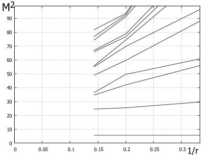
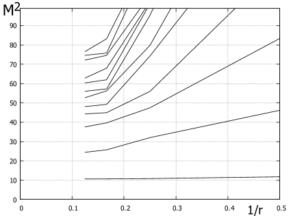
Figure 1: Bound state masses (squared) as a function of the (maximal) inverse parton number $1/r$ in the massless fermionic $T_{s}\pm$ and the massless bosonic $T_{s}+$ sectors.

Let’s take a look at the numerical results. We should first check convergence. As expected, convergence without pair creation is very good. In the isolated, fixed parton-number sectors we reach percent accuracy with ten states or less, at least for the lowest states. On the other hand, convergence with parton number is problematic in the massless sectors of the theory. Fig. 1 shows that the ground state has well, the first excited state somewhat converged by the time the seven(eight) parton sector has been included in the fermionic(bosonic) sectors. The higher states have sizable contributions from higher parton sectors, although some of the higher bosonic masses seem pretty well converged by $r=8$. This is what we predicted in Sec. 4.1, where we found that the lowest asymptotic fermionic states have masses independent of parton number, whereas the masses of their bosonic counterparts grow linearly with $r$, suppressing mixing.

Things look quite differently in the massive theory, Fig. 3(a). At the supersymmetric point $m=\frac{g^{2}N}{\pi}$, most masses have converged after three parton sectors have been included. Apparently, it is energetically expensive to create parton pairs, and the asymptotic spectrum is a good approximation of the full solution.

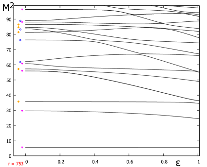
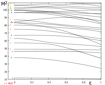
Figure 2: Bound state masses (squared) as a function of the parton-number violation parameter $\varepsilon$ in the massless fermionic $T_{s}\pm$ and the massless bosonic $T_{s}+$ sectors; the eigenvalue trajectories in the massive sectors are essentially horizontal lines.

6.1 The Massless Theory

Just how important is pair creation in the massless theory? If we plot masses as a function of the parton-number violation parameter $\varepsilon$, where the asymptotic(full) theory has $\varepsilon=0(1)$, Fig. 2, we see that some states’ masses are quite insensitive, while others depend substantially on $\varepsilon$. In fact, there seems to be a cascade of $\varepsilon$-dependent states. These states are impure in parton number, and intriguingly some of them have been identified previously [14, 3] as threshold bound states, i.e. multi-particle states. For instance, the second lowest bosonic state in Fig. 2, which starts out (as depicted in the left portion of the graph) as a four-parton state, has a 19%, 57%, 17%, 2% probability to be a 2, 4, 6, 8 parton state. The pattern continues at higher masses. It seems thus that there are two types of states. It is not clear what mechanism is at work to protect the pure states by heavily mixing the impure states. It could be that the impure states decouple from the rest of the spectrum in the large parton limit or, in DLCQ, in the continuum limit. It would be interesting to apply eLCQ to the bosonized theory to see whether the approximate multi-particle states decouple (as in: they are present in [17] only because the continuum limit has not been taken), or whether they are a genuine part of the theory.

Judging from the results at hand, eLCQ has limited capabilities to contribute positively to the debate about the massless theory. That said, it does provide evidence that the massless theory has a very different spectrum because its asymptotic eigenstates are in crucial aspects different from their massive counterparts. As we will see later, eLCQ also points to a problem of other approaches with the massless theory: due to its singularities it becomes near impossible to produce accurate, quantitative results with a simple, rigid IR regulator such as DLCQ.

6.2 The massive theory and the supersymmetric point

The massive theory’s spectrum is quite different from its massless counterpart which may shed some light on the controversy as to whether the massless theory is screening or confining [3, 2]. Note that we argue here from a basis function point of view. This may seem naive, but keep in mind that it is the physics (e.g. representation of fields) that determines the “boundary conditions” and therefore the appropriate set of basis states.

In the massive regime, all excitation numbers are even integers; the odd excitation numbers of the bosonic massless states would make it impossible to match fermionic and bosonic mass eigenvalues. All massive eigenfunctions are built form the same trig function, whereas in the massless sectors they are opposite (sine goes with cosine in the adjacent parton sector). Without this feature (following automatically from the symmetry structure of the theory) a supersymmetric point at $m=\frac{g^{2}N}{\pi}$ would be impossible.

The massive sectors have the least symmetric states, i.e. most disjunct statelets, which makes computing matrix elements expensive. On the positive side, the asymptotic eigenstates are very good approximations to the full eigenstates; the diagonal Hamiltonian matrix blocks (singular, regular, mass terms) are dominated by their diagonal elements, whereas the pair-creation matrix elements are small. Hence, there is very little coupling between sectors of different parton number (observe the flatness of the eigenvalue trajectories in Fig. 3(a)), but also states with the same parton number hardly mix. Note that this feature is mostly independent of the mass of the fermions, as the singular and regular blocks just depend on the symmetry quantum numbers $TIS$, not on mass. In other words, there is a non-continuous difference between the massive and massless theory, favoring a different (screening) behavior of the latter.

Can we understand this qualitatively? After all, we are saying that a two-parton bosonic state yields the same (diagonal) element as a three-parton fermionic state. We consider the lowest states as the simplest case without loss of generality, since we need to have one-to-one matching of quasi-isolated states. From the singular, regular and mass term contributions we gather $23.2+0+6.2\mu=29.8$ as a crude estimate for the lowest two-parton mass in units $g^{2}N/\pi$ (true: 26.7), whereas for the three-parton state we have $14.4+3.7+11.3\mu=29.4$, so this agrees pretty well. The mechanism behind this “adjustment” of singular, regular and mass contributions is not obvious. Consider that in order to obtain the matrix elements, we integrate a single-variable sine over a one-dimensional domain vs. a $\sin\pi(n_{1}x_{1}+n_{2}x_{2})$ over a much more complicated domain. Of course, supersymmetry guarantees this degeneracy of fermion and boson masses, as shown in Ref. [7] by using the supersymmetric generator $G_{0}$. Nonetheless, it is amusing to watch this unfold numerically — even though it is the equivalent of showing (by group theory) that the product two rotations around two different axes is always a rotation.

Overall, eLCQ works well for the massive theory. To a fair approximation the asymptotic states describe the solutions of the full theory, and the supersymmetric degeneracy of boson and fermion bound-state masses is reproduced.

Figure 3: (a) Convergence and comparison of fermionic (left) and bosonic (right) eigenvalues at the supersymmetric point ($m=\frac{g^{2}N}{\pi}$ or $\mu=1$) as a function of inverse parton number $1/r$. Discrepancy of corresponding eigenvalues is at most 1.5%. (b) Comparison of DLCQ and eLCQ bound state masses (squared) in the asymptotic massive six parton sector with $T+$ and $\mu=4$. DLCQ results are dots plotted as a function of inverse harmonic resolution $1/K$; eLCQ results appear as squares at infinite resolution. Linear fits (dashed lines) to the DLCQ masses at highest $K$ agree well with eLCQ. Quadratic fits to data up to $K=24$ lead to unreasonable results, even though the behavior of the lowest three mass trajectories appears consistent.

7 Discussion and Conclusion

In this work we presented a complementary calculation of the spectrum of two-dimensioal adjoint QCD. By using a basis-function approach based on the asymptotic spectrum of the theory generated via the eLCQ algorithm, we work in the (momentum) continuum limit. The Achilles heel of the method is the relatively small number of parton sectors in which the Hamiltonian matrix elements can be calculated — at least by brute force methods. Leveraging the insights gained in the construction of the complete asymptotic eigenfunction spectrum, we understand that this is not a problem in the massive theory $m>0$, where pair creation is unimportant. In the massless theory we find states whose asymptotic masses are independent of parton number. We therefore expect the generic eigenstate in this sector to have substantial contributions from all parton sectors. As first noticed in [8], this is not the case for the lowest states; they are pure in parton number. This can be understood via eLCQ from the severe constraints of possible excitation numbers allowed by the symmetries of the theory. These symmetries explain the properties of the lowest states in remarkable detail, allowing for a good estimate of the masses, even though the asymptotic approximation assumes high excitation numbers.

Overall, our results are in fair agreement with previous DLCQ-based work [14, 3]. This shows that discretization or compactification of the theory yields qualitatively correct results, even if accuracy of bound-state masses becomes an issue. Note that in DLCQ(eLCQ) mass trajectories increase(decrease) as one approaches the continuum(infinite parton number) limit. In this light, it is concerning that there is a discrepancy even in the ground state mass

$$M^{2}_{F0}=5.72|_{DLCQ}\frac{g^{2}N}{\pi}\geq 5.69|_{eLCQ}\frac{g^{2}N}{\pi}.$$

After completing this work, we appreciate the great advantage of DLCQ to consistently (if coarsely at available $K$) approximating all states, which results in a faithful representation of the underlying algebraic structure. This is paramount for representation theory analyses [3, 4], and barring any improvements on the eLCQ approach, might be more important than accurately describing the eigenstates at low parton number. If the advantages of the two methods could be combined, one would have a powerful tool to analyze low-dimensional field theories!

In the meantime, we should point out the pitfalls in both approaches. Take a look at Fig. 3 depicting the masses of six-parton states when one neglects pair creation but includes all other interactions. Note that this is in the massive theory, so the former is actually a good approximation even in eLCQ. In Fig. 3 the DLCQ continuum limit cannot be taken if one has data only for $K<26$. The lowest states do not split off until a crucial resolution is reached; for higher states this resolution is obviously higher. In fact, at $r=7$, the condition has worsened to the point that this split (and hence the possibility of extrapolation) does not happen until one is forced to use sparse matrix methods (roughly 10,000 states at $K\geq 41$). Note that these large resolutions are not possible when all parton sectors are included. Fig. 3 also shows that eLCQ does get it right. Its limitation is that it essentially stops working at nine partons due to the exponentially growing numbers of terms in the Hamiltonian and statelets.

As mentioned, the conclusions of [3, 4] do not depend on the precise masses, but rather on the consistent, qualitative features of the spectrum and the relations (degeneracies) across different sectors of the theory. For eLCQ one might think of going to higher parton sectors by stochastically sampling statelets and terms.

Let us briefly discuss potential problems of discretized approaches at finite resolution — which are surprisingly benign as far as we can tell from comparing eLCQ and DLCQ results. To expose problems, we consider a hybrid method (“hLCQ”), where we take a DLCQ Hamiltonian matrix and sandwich it between eLCQ continuous asymptotic eigenfunctions. One then finds that there is a crucial discrepancy between the matrix elements computed in the two schemes. The hybrid method fools us into diagnosing a linear convergence in $1/K$ of the matrix elements towards a much smaller value than the (correct) one obtained analytically via the eLCQ algorithm. We can trace the dominant contributions to the matrix elements to integrals of the form $\int^{1}_{0}\cos(\pi(n^{\prime}-n_{3})x){\rm Si}(\pi n_{1}x)dx$ in which one of the incoming excitation numbers $n_{i}$ is equal to the outgoing $n^{\prime}$. These expressions result from similar integrals in the function $I_{PNV}(x_{1},y_{1})$, see appendix, which is diverging whenever $y_{1}=0$, while its integral over $y_{1}$ has only isolated divergences that will eventually cancel. It is clear, that any numerical integration — let alone a multi-dimensional one — will have poor outcomes. It is surprising that these issues with matrix elements in DLCQ do not have more severe consequences. It must be that there is a partial cancellation of errors which likely stems from the highest virtue of DLCQ: consistent approximations in all parton sectors.

In conclusion, the application of the eLCQ algorithm to QCD_2A generates a continuous (at fixed parton number) method to compute the spectrum of the theory. It is complementary to discretized approaches, and validates certain findings within these frameworks. While working in the continuum allows us to address some issues with using the light-cone gauge in a discretized formulation [2], problems connected to the Hamiltonian itself are beyond the scope of the present work. Since eLCQ is limited to small parton numbers, it would be interesting to apply it to the bosonized version of QCD_2A, where the effective parton number is essentially halved. It is not clear if this is feasible due to the symmetries being compromised by the Kac-Moody commutator. In general, however, one should be able with the present approach to figure out more easily which (formulations of) theories result in eigenstates pure in parton number, and for which pair production is crucial.

Appendix A Evaluating Matrix Elements I — General Method

We now apply the results of Sec. 5, i.e. the enlarged integral domain, to evaluating the matrix elements for arbitrary parton number $r$ with the spectator variables $\vec{x}_{Sp}$ and $\vec{y}_{Sp}$. We start with

$$\langle\vec{\mu}_{r}|\hat{H}_{0}|{\vec{\nu}_{r}}\rangle\!\!\! = \!\!\!\int_{cHS}\!\!d\vec{x}\int_{cHS}\!\!d\vec{y}\,\,\delta(x_{1}+x_{2}-y_{1}-y_{2})\delta^{r-3}(\vec{x}_{Sp}-\vec{y}_{Sp})\frac{[\phi(\vec{x})-\phi(\vec{y})]_{\mu\nu}}{(x_{1}-y_{1})^{2}}$$ (30)

$$= \!\!\!\int_{0}^{1}\!\!\!dx_{1}\int_{0}^{1-x_{1}}\!\!\!\!dx_{2}\int d^{r-3}\vec{x}_{Sp}\int_{0}^{x_{1}+x_{2}}\!\!\!dy_{1}\frac{[\phi(\vec{x})-\phi(\vec{y})]_{\mu\nu}}{(x_{1}-y_{1})^{2}}\Big{|}_{y_{2}=x_{1}+x_{2}-y_{1}\atop{\!\!\!\!\!\!\!\!\!\!\!\!\!\!\vec{y}_{Sp}=\vec{x}_{Sp}}},$$

where the upper limit on the last integral follows from $y_{2}\geq 0$. To split off the non-interacting partons (spectators), we have to commit to the actual form of our eigenfunctions, cf. Eq. (22)

$$\phi_{I+,\nu}={\cal N}\sum_{g\in{\cal G}}\cos\left(\pi g\vec{\nu}\!\cdot\!\vec{x}\right)\qquad\mbox{ or }\qquad\phi_{I-,\nu}={\cal N}\sum_{g\in{\cal G}}\sin\left(\pi g\vec{\nu}\!\cdot\!\vec{x}\right).$$

To simplify notation, call $(g\nu)_{i}\equiv n_{i}$, and use the sum-to-product trig identities to split off the spectator variables $\vec{x}_{Sp}$ and $\vec{y}_{Sp}$ in the double difference $[\phi(\vec{x})-\phi(\vec{y})]_{\mu\nu}$, Eq. (27). This leads to

$$[\phi(\vec{x})-\phi(\vec{y})]^{+}_{\mu\nu} = \frac{1}{2}\left[\left\{\cos\pi(m_{1}x_{1}+m_{2}x_{2})-\cos\pi(m_{1}y_{1}+m_{2}y_{2})\right\}\cos\pi\vec{m}\!\cdot\!\vec{x}_{Sp}\right.$$

$$\quad-\left.\left\{\sin\pi(m_{1}x_{1}+m_{2}x_{2})-\sin\pi(m_{1}y_{1}+m_{2}y_{2})\right\}\sin\pi\vec{m}\!\cdot\!\vec{x}_{Sp}\right]$$

$$\times\left[\left\{\cos\pi(n_{1}x_{1}+n_{2}x_{2})-\cos\pi(n_{1}y_{1}+n_{2}y_{2})\right\}\cos\pi\vec{n}\!\cdot\!\vec{x}_{Sp}\right.$$

$$\quad-\left.\left\{\sin\pi(n_{1}x_{1}+n_{2}x_{2})-\sin\pi(n_{1}y_{1}+n_{2}y_{2})\right\}\sin\pi\vec{n}\!\cdot\!\vec{x}_{Sp}\right],$$

and similar for $\phi_{I-}$, where we set $\vec{x}_{Sp}=\vec{y}_{Sp}$ due to the second delta function in Eq. (30). So we get four terms for $I+$ (and similar for $I-$)

$$[\phi(\vec{x})-\phi(\vec{y})]^{+}_{\mu\nu} \!\!\!\!=\!\!\!\! D^{00}_{\bar{\mu}\bar{\nu}}\cos\pi\vec{m}\!\cdot\!\vec{x}_{Sp}\cos\pi\vec{n}\!\cdot\!\vec{x}_{Sp}-D^{01}_{\bar{\mu}\bar{\nu}}\cos\pi\vec{m}\!\cdot\!\vec{x}_{Sp}\sin\pi\vec{n}\!\cdot\!\vec{x}_{Sp}$$

$$\!\!\!\!-D^{10}_{\bar{\mu}\bar{\nu}}\sin\pi\vec{m}\!\cdot\!\vec{x}_{Sp}\cos\pi\vec{n}\!\cdot\!\vec{x}_{Sp}+D^{11}_{\bar{\mu}\bar{\nu}}\sin\pi\vec{m}\!\cdot\!\vec{x}_{Sp}\sin\pi\vec{n}\!\cdot\!\vec{x}_{Sp},$$

where the double differences are defined as

$$D^{00}_{\bar{\mu}\bar{\nu}}(x_{1},x_{2},y_{1}) := \frac{1}{2}\left\{\cos\pi(m_{1}x_{1}+m_{2}x_{2})-\cos\pi(m_{1}y_{1}+m_{2}y_{2})\right\}$$

$$\times\left\{\cos\pi(n_{1}x_{1}+n_{2}x_{2})-\cos\pi(n_{1}y_{1}+n_{2}y_{2})\right\},$$

$$D^{01}_{\bar{\mu}\bar{\nu}}(x_{1},x_{2},y_{1}) \!\!\!:=\!\!\! \frac{1}{2}\left\{\cos\pi(m_{1}x_{1}+m_{2}x_{2})-\cos\pi(m_{1}y_{1}+m_{2}y_{2})\right\}$$ (31)

$$\times\left\{\sin\pi(n_{1}x_{1}+n_{2}x_{2})-\sin\pi(n_{1}y_{1}+n_{2}y_{2})\right\},$$

etc., and $\bar{\mu}\bar{\nu}$ is short for $m_{1},m_{2},n_{1},n_{2}$. Recall $y_{2}=x_{1}+x_{2}-y_{1}$. Analytically integrating over $\vec{x}_{Sp}$ is straightforward if tedious for large $r$. We label the results as follows

$$F^{ab-}_{mn}(x_{1},x_{2}) := \int d^{r-3}\vec{x}_{Sp}\sin_{a}\left(\pi\vec{m}\!\cdot\!\vec{x}_{Sp}\right)\sin_{b}\left(\pi\vec{n}\!\cdot\!\vec{x}_{Sp}\right),$$ (32)

where $a,b\in\{0,1\}$, $\sin_{0}=\cos$, and $\sin_{1}=\cos$. Note that $F^{01-}_{mn}=F^{10-}_{nm}$. Letting $F^{ab+}_{mn}(x_{1},x_{2})=(-1)^{a+b}F^{1-a,1-b-}_{mn}(x_{1},x_{2})$, we are left with the three-dimensional integral

$$\langle\vec{\mu}_{r}|\hat{H}_{0}|{\vec{\nu}_{r}}\rangle^{\pm}=\sum_{g_{in},g_{out}\in{\cal G}}\sum_{a,b=0}^{1}\int_{0}^{1}dx_{1}\int_{0}^{1-x_{1}}\!\!\!\!dx_{2}F^{1-a,1-b\pm}_{(\vec{m},\vec{n})_{Sp}}(x_{1},x_{2})\int_{0}^{x_{1}+x_{2}}\!\!\!\!dy\frac{D^{ab}_{\bar{\mu}\bar{\nu}}(x_{1},x_{2},y)}{(x_{1}-y)^{2}}.$$ (33)

To evaluate the matrix element, we first integrate over the momentum $y$ exchanged between the interacting partons for various trig function combinations

$$\tilde{I}^{+,-,0}_{y}(x_{1},x_{2}):=\int_{0}^{x_{1}+x_{2}}dy\frac{D^{00,11,01}_{\bar{\mu}\bar{\nu}}(x_{1},x_{2},y)}{(x_{1}-y)^{2}}$$

To properly treat the singularities, the integrals are to be taken with the prescription

$$\int_{0}^{1}dx_{1}\int_{0}^{1-x_{1}}dx_{2}\int_{0}^{x_{1}+x_{2}}\!\!\!dy:=\lim_{\epsilon\rightarrow 0}\int_{0}^{1}dx_{1}\int_{0}^{1-x_{1}}dx_{2}\left(\int_{0}^{x_{1}-\epsilon}\!\!\!dy+\int^{x_{1}+x_{2}}_{x_{1}+\epsilon}\!\!\!dy\right).$$

In total we have in the $I+$ sector with $m_{\pm}:=m_{1}-m_{2}\pm(n_{1}-n_{2})$

$$\tilde{I}^{+}_{y}\!\!\!\! = \!\!\!-\frac{1}{x_{2}}[\cos\pi m_{1}(x_{1}+x_{2})\cos\pi n_{1}(x_{1}+x_{2})+\cos\pi(m_{1}x_{1}+m_{2}x_{2})\cos\pi(n_{1}x_{1}+n_{2}x_{2})$$

$$\qquad-\cos\pi(m_{1}x_{1}+m_{2}x_{2})\cos\pi n_{1}(x_{1}+x_{2})-\cos\pi(n_{1}x_{1}+n_{2}x_{2})\cos\pi m_{1}(x_{1}+x_{2})]$$

$$\!\!\!-\frac{1}{x_{1}}[\cos\pi m_{2}(x_{1}+x_{2})\cos\pi n_{2}(x_{1}+x_{2})+\cos\pi(m_{1}x_{1}+m_{2}x_{2})\cos\pi(n_{1}x_{1}+n_{2}x_{2})$$

$$\qquad-\cos\pi(m_{1}x_{1}+m_{2}x_{2})\cos\pi n_{2}(x_{1}+x_{2})-\cos\pi(n_{1}x_{1}+n_{2}x_{2})\cos\pi m_{2}(x_{1}+x_{2})]$$

$$\!\!\!-\frac{\pi}{2}\Big{\{}m_{+}\sin\pi((m_{1}+n_{1})x_{1}+(m_{2}+n_{2})x_{2})[{\rm Ci\,}\pi|m_{+}|x_{2}-{\rm Ci\,}\pi|m_{+}|x_{1}]$$

$$\!\!\!\qquad+m_{-}\sin\pi((m_{1}-n_{1})x_{1}+(m_{2}-n_{2})x_{2})[{\rm Ci\,}\pi|m_{-}|x_{2}-{\rm Ci\,}\pi|m_{-}|x_{1}]\Big{\}}$$

$$\!\!\!-\pi(n_{1}-n_{2})\cos\pi(m_{1}x_{1}+m_{2}x_{2})\sin\pi(n_{1}x_{1}+n_{2}x_{2})[{\rm Ci\,}\pi|n_{1}-n_{2}|x_{2}-{\rm Ci\,}\pi|n_{1}-n_{2}|x_{1}]$$

$$\!\!\!-\pi(m_{1}\!-\!m_{2})\cos\pi(n_{1}x_{1}\!+\!n_{2}x_{2})\sin\pi(m_{1}x_{1}\!+\!m_{2}x_{2})[{\rm Ci\,}\pi|m_{1}\!-\!m_{2}|x_{2}-{\rm Ci\,}\pi|m_{1}\!-\!m_{2}|x_{1}]$$

$$\!\!\!-\frac{\pi}{2}\Big{\{}\pi m_{+}\cos\pi((m_{1}+n_{1})x_{1}+(m_{2}+n_{2})x_{2})[{\rm Si\,}\pi m_{+}x_{2}+{\rm Si\,}\pi m_{+}x_{1})]$$

$$\qquad+m_{-}\cos\pi((m_{1}-n_{1})x_{1}+(m_{2}-n_{2})x_{2})[{\rm Si\,}\pi m_{-}x_{2}+{\rm Si\,}\pi m_{-}x_{1}]\Big{\}}$$

$$\!\!\!-\pi(n_{1}-n_{2})\cos\pi(m_{1}x_{1}+m_{2}x_{2})\cos\pi(n_{1}x_{1}+n_{2}x_{2})[{\rm Si\,}\pi(n_{1}-n_{2})x_{2}+{\rm Si\,}\pi(n_{1}-n_{2})x_{1}]$$

$$\!\!\!-\pi(m_{1}\!-\!m_{2})\cos\pi(n_{1}x_{1}\!+\!n_{2}x_{2})\cos\pi(m_{1}x_{1}\!+\!m_{2}x_{2})[{\rm Si\,}\pi(m_{1}\!-\!m_{2})x_{2}+{\rm Si\,}\pi(m_{1}\!-\!m_{2})x_{1}]$$

and similar for $\tilde{I}^{-}(x_{1},x_{2})$ and $\tilde{I}^{0}(x_{1},x_{2})$. We then assemble the full matrix elements by combining the $\tilde{I}_{y}(x_{1},x_{2})$ functions with the spectator functions $F^{ab}(x_{1},x_{2})$. The result are functions of $x_{1},x_{2}$ which involve powers, trig functions and logarithms.

Before we categorize and integrate those in the next section, we point out that Eq. (30) contains a redundancy which will allow us to save at least a factor of two in numerical effort. Namely, due to the fact that $x_{r}$ does not explicitly appear yet is present in the formalism (we went to great lengths in Sec. 5 to keep it out of calculations), we can replace the integral over $x_{r-1}$ with an integral over $x_{r}$ (same limits). This means that sandwiching the Hamiltonian between statelets that are cyclically rotated (on both in and out sides) such that $x_{r-1}$ and $x_{r}$ are permuted will yield the same result. For instance,

$$\langle\mu;0|\hat{H}|\nu;r-1\rangle=\langle\mu;0|\hat{H}{\cal C}^{r-1}|\nu;0\rangle=\langle\mu;0|{\cal C}^{r-1}\hat{H}|\nu;0\rangle=\langle\mu;r-1|\hat{H}|\nu;0\rangle,$$

where $|\nu;j\rangle$ is the $j$th statelet of the state characterized by the excitation tuplet $\nu$.

Appendix B Evaluating Matrix Elements II — Integrals

All matrix elements require us to integrate expressions of the form

$$\frac{{\rm sos}(\pi\vec{m}\!\cdot\!\vec{x})\,{\rm cin}(\pi\vec{n}\!\cdot\!\vec{y})}{(x_{1}\pm y_{1})^{2}}$$

over various domains of different dimensionality. All singularities are integrable if the integrals are carefully regulated and one evaluates only matrix elements between bona fide asymptotic states. In particular, matrix elements between statelets might still be singular, typically like $\ln\epsilon$ or $\ln\bar{\epsilon}$, where the former is a spatial, the latter a excitation number regulator. The four fundamental categories of integrals we encounter are

$$\int dx\,x^{n}\sin_{s}(\pi kx),\int dx\,x^{n}{\rm Si}_{S}(\pi qx),\int dx\,x^{n}\sin_{s}(\pi kx)\ln x,\int dx\,x^{n}\sin_{s}(\pi kx){\rm Si}_{S}(\pi qx),$$

where $s=0(1)$ denotes a $\cos(\sin)$ and $S=0(1)$ is a ${\rm Ci}({\rm Si})$. All matrix elements are linear combinations of integrals of these types, e.g. part of the “singular” matrix element

$$\int^{1}_{0}dx_{1}\,x_{1}^{n_{1}}\int^{1-x_{1}}_{0}dx_{2}\,x_{2}^{n_{2}}\sin_{s}(\pi(k_{1}x_{1}+k_{2}x_{2})){\rm Si}_{S}(\pi qx_{2}).$$ (34)

This makes sense, since integrating a double pole will lead to a single pole or a sine or cosine integral, while integrating again will turn the single pole into a logarithm (worst case). The powers of $x$ are generated by spectator integrals in the higher parton sectors if two excitation numbers are equal or opposite. We sketch the specific evaluations for singular, regular and parton-number violating interactions in the following subsections.

B.1 Fundamental Integrals

We need the following results

$$\int x^{n}\sin(\pi(a+kx))dx = \left(\sum_{j=1}^{n/2+1}\frac{(-1)^{j}}{(\pi k)^{2j-1}}\frac{n!}{(n-2j+2)!}x^{n-2j+2}\right)\cos(\pi(a+kx))$$ (35)

$$+\left(\sum_{j=1}^{(n+1)/2}\frac{(-1)^{j+1}}{(\pi k)^{2j}}\frac{n!}{(n-2j+1)!}x^{n-2j+1}\right)\sin(\pi(a+kx))$$

$$=: A_{n}(x)\cos(\pi(a+kx))+B_{n}(x)\sin(\pi(a+kx))$$

$$\int x^{n}\cos(\pi(a+kx))dx = -A_{n}(x)\sin(\pi(a+kx))+B_{n}(x)\cos(\pi(a+kx)),$$ (36)

where $A_{n}=:\sum_{j=1}^{n/2+1}a_{nj}x^{n-2j+2}$, etc.. These expressions have to be evaluated at the limits ($L:=1-\sum_{i=1}^{t}x_{i},0$) so that

$$\int_{0}^{L}x^{n}\sin(\pi(a+kx))dx = A_{n}(L)\cos(\pi(a+kL))-a_{n,n/2+1}(0)\cos(\pi a)$$

$$+B_{n}(L)\sin(\pi(a+kL))-b_{n,(n+1)/2}(0)\sin(\pi a),$$

where

$$a_{n,n/2+1}(0)=\frac{n!(-1)^{n/2+1}}{(\pi k)^{n+1}},\qquad b_{n,\frac{n+1}{2}}(0)=-\frac{n!(-1)^{\frac{n+1}{2}}}{(\pi k)^{n+1}}.$$

Note that at the lower limit there is only at most one (constant) term, since $j$ has to be such that the exponent of $x$ is zero.

For the second type of integrals we have ($\tilde{x}_{1}:=1-x_{1}$)

$$\int_{0}^{\tilde{x}_{1}}x^{n}{\rm Si}(\pi qx)dx\!\!\! = \!\!\!\frac{1}{n+1}\Big{[}\tilde{x}_{1}^{n+1}{\rm Si}(\pi q\tilde{x}_{1})+\frac{\tilde{x}_{1}^{n}}{\pi q}\Big{(}\cos(\pi q\tilde{x}_{1})-\delta^{n}_{0}\Big{)}-\frac{n\bar{\delta}^{n}_{0}}{\pi q}\int^{\tilde{x}_{1}}_{0}\!\!\!\!x^{n-1}\cos(\pi qx)dx\Big{]}$$

$$\int_{0}^{\tilde{x}_{1}}x^{n}{\rm Ci}(\pi qx)dx\!\!\! = \!\!\!\frac{\bar{\delta}^{q}_{0}}{n+1}\Big{[}\tilde{x}_{1}^{n+1}{\rm Ci}(\pi q\tilde{x}_{1})-\frac{\tilde{x}_{1}^{n}}{\pi q}\sin(\pi q\tilde{x}_{1})+\frac{n\bar{\delta}^{n}_{0}}{\pi q}\int^{\tilde{x}_{1}}_{0}x^{n-1}\sin(\pi qx)dx\Big{]}$$

$$+\frac{\delta^{q}_{0}}{n+1}\left(\gamma+\ln\pi\bar{\epsilon}+\ln\tilde{x}_{1}-\frac{1}{n+1}\right)\tilde{x}_{1}^{n+1}.$$

The third type of integrals can be written recursively as ($k\neq 0$)

$$\int_{0}^{\tilde{x}_{1}}dx\,x^{n}\sin(\pi kx)\ln x = L_{s}^{(n)}(\tilde{x}_{1})+\frac{n}{\pi k}\int^{\tilde{x}_{1}}_{0}x^{n-1}\cos(\pi kx)\ln x$$ (37)

$$\int^{\tilde{x}_{1}}_{0}dx\,x^{n}\cos(\pi kx)\ln x = L_{c}^{(n)}(\tilde{x}_{1})-\frac{n}{\pi k}\int^{\tilde{x}_{1}}_{0}x^{n-1}\sin(\pi kx)\ln x,$$

with the “rest” functions

$$L_{s}^{(n)}(\tilde{x}_{1}) = -\frac{\tilde{x}_{1}^{n}}{\pi k}\Big{[}\ln\tilde{x}_{1}\cos(\pi k\tilde{x}_{1})-\delta^{n}_{0}\Big{(}{\rm Ci}(\pi k\tilde{x}_{1})-\gamma-\ln\pi k\Big{)}\Big{]}$$

$$+\bar{\delta}^{n}_{0}\Big{[}\frac{\tilde{x}_{1}^{n-1}}{(\pi k)^{2}}\sin(\pi k\tilde{x}_{1})-\frac{(n-1)\bar{\delta}^{n}_{1}}{(\pi k)^{2}}\int^{\tilde{x}_{1}}_{0}x^{n-2}\sin(\pi kx)dx\Big{]}$$

$$L_{c}^{(n)}(\tilde{x}_{1}) = \frac{\tilde{x}_{1}^{n}}{\pi k}\Big{[}\ln\tilde{x}_{1}\sin(\pi k\tilde{x}_{1})-\delta^{n}_{0}{\rm Si}(\pi k\tilde{x}_{1})\Big{]}$$

$$+\bar{\delta}^{n}_{0}\Big{[}\frac{\tilde{x}_{1}^{n-1}}{(\pi k)^{2}}\Big{(}\cos(\pi k\tilde{x}_{1})-\delta^{n}_{1}\Big{)}-\frac{(n-1)\bar{\delta}^{n}_{1}}{(\pi k)^{2}}\int^{\tilde{x}_{1}}_{0}x^{n-2}\cos(\pi kx)dx\Big{]}.$$

Converting into sums yields

$$\int^{\tilde{x}_{1}}_{0}dx\,x^{n}\sin_{s}(\pi kx)\ln x=\bar{\delta}^{k}_{0}\sum_{j=0}^{n/2}\frac{n!}{(n-2j)!}\frac{(-1)^{j}}{(\pi k)^{2j}}\left(L_{s}^{(n-2j)}-(-1)^{s}\frac{n-2j}{\pi k}L_{1-s}^{(n-2j-1)}\right).$$

The last integral category is handled in the next subsection as part of an example for the calculation of matrix elements.

B.2 Singular Matrix Elements

For “singular” matrix elements one employs the enlarged integral domain of Sec. 5 which complicates the numerator of the integrals, i.e. requires more algebraic effort, but does not add to the list of integrals. Nonetheless, evaluation is very cumbersome, as one can see from computing the generic integral(s) Eq. (34) $\forall\,n_{1},n_{2}\geq 0,k_{1},k_{2},q\in\mathbb{Z}$ as well as $s,S\in\{0,1\}$. We can write the inner integral recursively as in Eq. (37) where the “rest” functions $R_{jJ}^{(n)}(\tilde{x}_{1})$ (replacing the $L^{(n)}_{j}$) are

$$2\pi kR_{sS}^{(n)}(\tilde{x}_{1}) = -2\tilde{x}_{1}^{n}\cos(\pi k\tilde{x}_{1}){\rm Si}(\pi q\tilde{x}_{1})\pm\sum_{\mp}\bar{\delta}^{k}_{\pm q}\Big{\{}\delta^{n}_{0}\,{\rm Si}(\pi(k\mp q)\tilde{x}_{1})+\bar{\delta}^{n}_{0}\,\Gamma_{\mp}(\tilde{x}_{1})\Big{\}}$$

$$2\pi kR_{cS}^{(n)}(\tilde{x}_{1}) = 2\tilde{x}_{1}^{n}\sin(\pi k\tilde{x}_{1}){\rm Si}(\pi q\tilde{x}_{1})-(\delta^{k}_{q}-\delta^{k}_{-q})\left(\frac{\bar{\delta}^{n}_{0}}{n}+\delta^{n}_{0}\ln\tilde{x}_{1}\right)\tilde{x}_{1}^{n}\Big{\}}$$

$$\mp\sum_{\mp}\bar{\delta}^{k}_{\pm q}\Big{\{}\delta^{n}_{0}\Big{[}{\rm Ci}(\pi|k\mp q|\tilde{x}_{1})-\gamma-\ln(\pi|k\mp q|)\Big{]}+\bar{\delta}^{n}_{0}\,\bar{\Gamma}_{\mp}(\tilde{x}_{1})\Big{\}}$$

$$R_{sC}^{(n)}(\tilde{x}_{1}) = \delta^{q}_{0}\Big{[}\left(\gamma+\ln(\pi\bar{\epsilon})\right)\int_{0}^{\tilde{x}_{1}}x^{n}\sin(\pi kx)dx+\int_{0}^{\tilde{x}_{1}}x^{n}\sin(\pi kx)\ln x\,dx\Big{]}$$

$$+\frac{\bar{\delta}^{q}_{0}}{2\pi k}\Bigg{\{}-2\tilde{x}_{1}^{n}\cos(\pi k\tilde{x}_{1}){\rm Ci}(\pi q\tilde{x}_{1})+(\delta^{k}_{q}+\delta^{k}_{-q})\left(\frac{\bar{\delta}^{n}_{0}}{n}+\delta^{n}_{0}\ln\tilde{x}_{1}\right)\tilde{x}_{1}^{n}\Bigg{\}}$$

$$+\sum_{\mp}\bar{\delta}^{k}_{\pm q}\Big{\{}\delta^{n}_{0}\tilde{x}_{1}^{n}\Big{[}{\rm Ci}(\pi|k\mp q|\tilde{x}_{1})-\gamma-\ln(\pi|k\mp q|)\Big{]}+\bar{\delta}^{n}_{0}\,\bar{\Gamma}_{\mp}(\tilde{x}_{1})\Big{\}}$$

$$R_{cC}^{(n)}(\tilde{x}_{1}) = \delta^{q}_{0}\Big{[}\left(\gamma+\ln(\pi\bar{\epsilon})\right)\int_{0}^{\tilde{x}_{1}}x^{n}\cos(\pi kx)dx+\int_{0}^{\tilde{x}_{1}}x^{n}\cos(\pi kx)\ln x\,dx\Big{]}$$

$$+\frac{\bar{\delta}^{q}_{0}}{2\pi k}\Bigg{\{}2\tilde{x}_{1}^{n}\sin(\pi k\tilde{x}_{1}){\rm Ci}(\pi q\tilde{x}_{1})-\sum_{\mp}\bar{\delta}^{k}_{\pm q}\Big{\{}\delta^{n}_{0}{\rm Si}(\pi(k\mp q)\tilde{x}_{1})-\bar{\delta}^{n}_{0}\,\Gamma_{\mp}(\tilde{x}_{1})\Big{\}},$$

where

$$\Gamma_{\mp}(\tilde{x}_{1}) := \frac{\tilde{x}_{1}^{n-1}}{\pi(k\mp q)}\left(\cos(\pi(k\mp q)\tilde{x}_{1})-\delta^{n}_{1}\right)-\frac{(n-1)\bar{\delta}^{n}_{1}}{\pi(k\mp q)}\int^{\tilde{x}_{1}}_{0}x^{n-2}\cos(\pi(k\mp q)x)dx,$$

$$\bar{\Gamma}_{\mp}(\tilde{x}_{1}) := \frac{\tilde{x}_{1}^{n-1}}{\pi(k\mp q)}\sin(\pi(k\mp q)\tilde{x}_{1})-\frac{(n-1)\bar{\delta}^{n}_{1}}{\pi(k\mp q)}\int^{\tilde{x}_{1}}_{0}x^{n-2}\sin(\pi(k\mp q)x)dx.$$

The integrals in these expressions are sums of powers of $\tilde{x}_{1}$ and trig functions, Eqs. (35) plus integrals with an additional logarithm. In other words, integrals of categories one and three. Then

$$\int^{\tilde{x}_{1}}_{0}\!\!\!\!dx\,x^{n}\sin_{s}(\pi kx){\rm Si}_{S}(\pi qx)\!\!\! = \!\!\!\bar{\delta}^{k}_{0}\sum_{j=0}^{n/2}\frac{n!}{(n-2j)!}\frac{(-1)^{j}}{(\pi k)^{2j}}\left(R_{sS}^{(n-2j)}-(-)^{s}\frac{n-2j}{\pi k}R_{1-s,S}^{(n-2j-1)}\right)$$

$$+\delta^{k}_{0}\delta^{s}_{0}\int_{0}^{\tilde{x}_{1}}dx\,x^{n}{\rm Si}_{S}(\pi qx).$$

With the inner integral evaluated, we can now use

$$\int^{1}_{0}x_{1}^{n}\sin_{s}(\pi k_{1}x_{1})f(1-x_{1})dx_{1}=\sum_{p=0}^{n}(-1)^{k_{1}+s+p}\left({n\atop p}\right)\int_{0}^{1}\tilde{x}^{p}_{1}\sin_{s}(\pi k_{1}\tilde{x}_{1})f(\tilde{x}_{1})d\tilde{x}_{1}$$

and the occasional trig identity to write our integral (34) as a linear combination of the four categorized integrals above.

B.3 Regular Matrix Elements

By comparison, the regular parton-number conserving interaction is easy to deal with, since the term looks like

$$\frac{g^{2}N}{\pi(x_{1}+x_{2})^{2}}\int_{0}^{x_{1}+x_{2}}dy\,\phi(y,x_{1}+x_{2}-y,x_{3},...x_{b}).$$

It is easy to see that the term vanishes for $r=2$. The general result ($r>3$) is essentially the integral

$$\int_{0}^{x_{1}+x_{2}}dy\,\sin_{s}\pi(n_{1}-n_{2})y=(-1)^{s}\left[\frac{1}{\pi(n_{1}-n_{2})}\sin_{1-s}(\pi(n_{1}-n_{2})(x_{1}+x_{2}))-\delta^{s}_{0}\right].$$

The projection integral is cumbersome since we pick up the factor $\frac{1}{(x_{1}+x_{2})^{2}}$ which becomes part of the $x_{1}$ and $x_{2}$ integrations and is singular at the lower limit. As before, we assume the spectator momenta have been separated and integrated out, producing linear combinations of polynomials and sinusoidals of $x_{1}$ and $x_{2}$, such that the arising types of integrals are limited to

$$\int_{0}^{1}dx_{1}\int^{1-x_{1}}_{0}dx_{2}\frac{\sin_{s}(\pi(k_{1}x_{1}+k_{2}x_{2})}{(x_{1}+x_{2})^{n}},\qquad n=0,1,2;k_{i}\in\mathbb{Z}.$$

Note that the asymptotically massless fermionic states $|0^{r-1}\rangle$ have a regular matrix element $\langle 0^{r-1}|\hat{H}_{PC}|0^{r-1}\rangle$ that is easily calculated due to

$$\int_{0}^{1}dx_{1}\int_{0}^{1-x_{1}}dx_{2}\frac{1}{x_{1}+x_{2}}\int_{0}^{1-x_{1}-x_{2}}dx_{3}\cdots\int_{0}^{1-\sum_{j}^{r-2}x_{i}}dx_{r-1}=\frac{1}{(r-2)!}.$$

The norm for these constant states is the square-root of the inverse integration volume $r!$, so we obtain Eq. (29), which leads, as pointed out above, to a good estimate for the ground state masses in the fermionic sectors.

B.4 Parton-Number Violating Matrix Elements

The calculation of the parton-number violating matrix elements involves integrals similar to the regular matrix elements of Appx. B.3. To wit, for incoming cosines we have

$$\int_{0}^{1}dx_{1}\int_{0}^{1}dy_{1}\int_{0}^{1-y_{1}}dy_{2}\int_{0}^{1-y_{1}-y_{2}}dy_{3}\cos\pi m_{1}x_{1}\cos\pi(n_{1}y_{1}+n_{2}y_{2}+n_{3}y_{3})$$

$$\qquad\qquad\qquad\qquad\qquad\times\left[\frac{1}{(y_{1}+y_{2})^{2}}-\frac{1}{(y_{2}+y_{3})^{2}}\right]\delta(x_{1}-y_{1}-y_{2}-y_{3})$$

$$=\int_{0}^{1}dx_{1}\cos\pi m_{1}x_{1}\int_{0}^{x_{1}}dy_{1}\left[I_{PNV,1c}(x_{1},y_{1})-I_{PNV,2c}(x_{1},y_{1})\right],$$

where

$$I^{(n_{2}=n_{3})}_{PNV,1c}(x_{1},y_{1})\!\! := \cos\pi(n_{3}x_{1}+(n_{1}-n_{3})y_{1})\left[\frac{1}{y_{1}}-\frac{1}{x_{1}}\right]$$ (38)

$$I^{(n_{2}\neq n_{3})}_{PNV,1c}(x_{1},y_{1})\!\! := \frac{\cos\pi(n_{3}x_{1}\!+\!(n_{1}\!-\!n_{3})y_{1})}{y_{1}}-\frac{\cos\pi(n_{2}x_{1}\!+\!(n_{1}\!-\!n_{2})y_{1})}{x_{1}}-\pi(n_{2}\!-\!n_{3})$$

$$\times\left\{\cos\pi((n_{2}-n_{1})y_{1}-n_{3}x_{1})[{\rm Si}(\pi(n_{2}-n_{3})x_{1})-{\rm Si}(\pi(n_{2}-n_{3})y_{1})]\right.$$

$$\left.\qquad\!\!\!-\sin\pi((n_{2}\!-\!n_{1})y_{1}\!-\!n_{3}x_{1})[{\rm Ci}(\pi(n_{2}\!-\!n_{3})x_{1})-{\rm Ci}(\pi(n_{2}\!-\!n_{3})y_{1})]\right\}$$

$$I^{(n_{2}\neq n_{3})}_{PNV,2c}(x_{1},y_{1}) := \frac{1}{\pi(n_{3}-n_{2})}\frac{\sin\pi(n_{3}x_{1}+(n_{1}-n_{3})y_{1})}{(x_{1}-y_{1})^{2}}+(n_{2}\leftrightarrow n_{3})$$ (39)

$$I^{(n_{2}=n_{3})}_{PNV,2c}(x_{1},y_{1}) := \frac{\cos\pi(n_{3}x_{1}+(n_{1}-n_{3})y_{1})}{x_{1}-y_{1}}.$$ (40)

The next step is the $y_{1}$ integration which yields

$$\int_{\epsilon}^{x_{1}}\!\!\!I^{(n_{2}=n_{3},n_{1}\neq n_{3})}_{PNV,1c}dy_{1}\!\!\! = \frac{1}{\pi(n_{1}-n_{3})}\frac{\sin\pi n_{3}x_{1}-\sin\pi n_{1}x_{1}}{x_{1}}-\sin\pi n_{3}x_{1}{\rm Si}(\pi(n_{1}-n_{3})x_{1})$$

$$+\cos\pi n_{3}x_{1}[{\rm Ci}(\pi(n_{1}-n_{3})x_{1})-{\rm Ci}(\pi(n_{1}-n_{3})\epsilon)]$$

$$\int_{\epsilon}^{x_{1}}\!\!\!I^{(n_{2}=n_{3},n_{1}=n_{3})}_{PNV,1c}dy_{1}\!\!\! = \cos\pi n_{3}x_{1}[\ln x_{1}-\ln\epsilon-1]$$

$$\int_{\epsilon}^{x_{1}}\!\!\!I^{(n_{2}\neq n_{3},n_{2}\neq n_{1})}_{PNV,1c}dy_{1}\!\!\! = \!\!\!\delta^{n_{1}}_{n_{3}}\cos\pi n_{3}x_{1}[\ln x_{1}-\ln\epsilon]-\bar{\delta}^{n_{1}}_{n_{3}}\Big{\{}\sin(\pi n_{3}x_{1}){\rm Si}(\pi(n_{1}-n_{3})x_{1})$$

$$\qquad\qquad\qquad-\cos(\pi n_{3}x_{1})[{\rm Ci}(\pi(n_{1}-n_{3})x_{1})-{\rm Ci}(\pi(n_{1}-n_{3})\epsilon)]\Big{\}}$$

$$\!\!\!+\frac{\sin(\pi n_{1}x_{1})-\sin(\pi n_{2}x_{1})}{\pi(n_{2}-n_{1})x_{1}}$$

$$\!\!\!-\pi(n_{2}\!-\!n_{3})\Bigg{[}\frac{{\rm Si}(\pi(n_{2}-n_{3})x_{1})}{\pi(n_{2}-n_{1})}[\sin(\pi(n_{2}-n_{1}-n_{3})x_{1})-\sin(\pi n_{3}x_{1})]$$

$$\qquad\qquad\qquad\qquad-I_{cS}(x_{1},n_{2}-n_{1},n_{2}-n_{3},-n_{3}x_{1})$$

$$\qquad\qquad\,\,\,+\frac{{\rm Ci}(\pi(n_{2}-n_{3})x_{1})}{\pi(n_{2}-n_{1})}[\cos(\pi(n_{2}\!-\!n_{1}\!-\!n_{3})x_{1})-\cos(\pi n_{3}x_{1})]$$

$$\qquad\qquad\qquad\qquad+I_{sC}(x_{1},n_{2}-n_{1},n_{2}-n_{3},-n_{3}x_{1})\Bigg{]}$$

$$\int_{\epsilon}^{x_{1}}\!\!\!I^{(n_{2}\neq n_{3},n_{2}=n_{1})}_{PNV,1c}dy_{1} = \cos(\pi n_{3}x_{1})[{\rm Ci}(\pi(n_{1}-n_{3})x_{1})-{\rm Ci}(\pi(n_{1}-n_{3})\epsilon)]$$

$$-\sin(\pi n_{3}x_{1}){\rm Si}(\pi(n_{1}-n_{3})x_{1})-\cos(\pi n_{2}x_{1})$$

$$+\cos(\pi n_{3}x_{1})[\cos(\pi(n_{2}\!-\!n_{3})x_{1})\!-\!1]-\sin(\pi n_{3}x_{1})\sin(\pi(n_{2}\!-\!n_{3})x_{1}),$$

where

$$I_{sS}(k,q,b)=\int_{0}^{x}\sin_{s}(\pi(kx^{\prime}+b)){\rm Si}_{S}(\pi qx^{\prime})dx^{\prime}.$$

The contributions from the second terms, Eqs. (B.4)&(40), are similar, but only contribute when $n_{1}\neq n_{3}$. Incidentally, a multi-dimensional numerical integration might have trouble converging, since one integrates divergent functions in intermediate steps. For incoming sine wavefunctions we obtain similar results.

From the expressions it is clear that the final integration over $x_{1}$ can be expressed in terms of definite integrals of the four types discussed above. The simplest are

$$D_{cC}(k,q)\!:=\!\int_{0}^{1}\cos(\pi kx){\rm Ci}(\pi qx)dx\!\! = \!\!\frac{\bar{\delta}^{k}_{0}}{2\pi k}\left[{\rm Si}(\pi(k-q))+{\rm Si}(\pi(k+q))\right]+\delta^{k}_{0}{\rm Ci}(\pi q)$$

$$D_{sS}(k,q)\!:=\!\int_{0}^{1}\sin(\pi kx){\rm Si}(\pi qx)dx\!\! = \!\!\frac{\bar{\delta}_{0}^{k}}{2\pi k}\left[{\rm Si}(\pi(k\!-\!q))-{\rm Si}(\pi(k\!+\!q))+2(-)^{k}{\rm Si}(\pi q)\right]$$

$$D_{cS}(k,q)\!:=\!\int_{0}^{1}\cos(\pi kx){\rm Si}(\pi qx)dx\!\! = \!\!\frac{\bar{\delta}^{k}_{0}}{2\pi k}\Big{[}{\rm Ci}(\pi|k-q|)-{\rm Ci}(\pi|k+q|)$$

$$\left.-\ln\left|\frac{k-q}{k+q}\right|\right]+\delta^{k}_{0}\left[{\rm Si}(\pi q)+\frac{(-1)^{q}-1}{\pi q}\right]$$

$$D_{sC}(k,q)\!:=\!\int_{0}^{1}\sin(\pi kx){\rm Ci}(\pi qx)dx\!\! = \!\!\frac{1-\delta^{k}_{0}}{2\pi k}\Big{[}{\rm Ci}(\pi|k-q|)+{\rm Ci}(\pi|k+q|)$$

$$\left.-2{\rm Ci}(\pi|q|)(-1)^{k}-\ln\left|\frac{k^{2}}{q^{2}}-1\right|\right].$$

Note that $D_{cC}(0,q\rightarrow 0)=\gamma+\ln(\pi q)-1$ is divergent, whereas

$$D_{sC}(k,0)=\frac{1}{\pi k}\left[{\rm Ci}(\pi|k|)-\ln|k|-(-1)^{k}(\gamma+\ln\pi)-\ln q((-1)^{k}-1)\right]$$

is finite only for even $k$.

B.5 Mass Term Elements

The mass term elements are dramatically simplified by using the union of all unique Hilbert spaces, cHS, as the integration domain, see Sec. 5. They read

$$\langle\vec{\mu}|\hat{H}_{m}|\vec{\nu}\rangle=\frac{m^{2}}{2}\int_{0}^{1}\frac{dx_{1}}{x_{1}}\int_{0}^{1-x_{1}}dx_{2}\cdots\int_{0}^{1-\sum_{i}^{r-1}x_{i}}dx_{r-1}\sin_{I}(\pi\vec{\mu}\cdot\vec{x})\sin_{I}(\pi\vec{\nu}\cdot\vec{x}),$$

where $I$ is the ${\cal I}$ quantum number of the sector, $\sin_{-1}=\sin$, and $\sin_{+1}=\cos$.

References

- [1] E. Katz, G. M. Tavares and Y. Xu, JHEP 1405 (2014) 143.
- [2] A. Cherman, T. Jacobson, Y. Tanizaki and M. Ünsal, SciPost Phys. 8 (2020) no.5, 072.
- [3] R. Dempsey, I. R. Klebanov and S. S. Pufu, JHEP 10 (2021), 096.
- [4] R. Dempsey, I. R. Klebanov, L. L. Lin and S. S. Pufu, JHEP 04 (2023), 107.
- [5] R. Gopakumar, A. Hashimoto, I. R. Klebanov, S. Sachdev and K. Schoutens, Phys. Rev. D 86 (2012) 066003.
- [6] F. Antonuccio and S. Pinsky, Phys. Lett. B 439 (1998) 142.
- [7] D. Kutasov, Nucl. Phys. B414 (1994) 33.
- [8] S. Dalley and I. R. Klebanov, Phys. Rev. D 47 (1993) 2517.
- [9] G. Bhanot, K. Demeterfi and I. R. Klebanov, Phys. Rev. D 48 (1993) 4980.
- [10] A. V. Smilga, SciPost Phys. 10 (2021) no.6, 152.
- [11] D. J. Gross, I. R. Klebanov, A. V. Matytsin and A. V. Smilga, Nucl. Phys. B 461 (1996), 109-130.
- [12] G. ’t Hooft, Nucl. Phys. B 75 (1974) 461.
- [13] D. Kutasov and A. Schwimmer, Nucl. Phys. B 442 (1995) 447.
- [14] D. J. Gross, A. Hashimoto and I. R. Klebanov, Phys. Rev. D 57 (1998) 6420.
- [15] Z. Komargodski, K. Ohmori, K. Roumpedakis and S. Seifnashri, JHEP 03 (2021), 103.
- [16] A. Armoni, Y. Frishman and J. Sonnenschein, Nucl. Phys. B 596 (2001), 459-470.
- [17] U. Trittmann, Nucl. Phys. B 587, 311 (2000), Phys. Rev. D 66, 025001 (2002).
- [18] U. Trittmann, Phys. Rev. D 92, 085021 (2015).
- [19] U. Trittmann, Phys. Rev. D 98, 045011 (2018).
- [20] G. McCartor, D. G. Robertson and S. S. Pinsky, Phys. Rev. D 56 (1997), 1035-1049.
- [21] E. Witten, Commun. Math. Phys. 92, 455-472 (1984).
- [22] I.R. Klebanov, private communication.
- [23] D. Delmastro, J. Gomis and M. Yu, JHEP 02 (2023), 157; D. Delmastro and J. Gomis, [arXiv:2211.09036 [hep-th]].