Finite Stature in Artin groups

Abstract.

We give criteria for a graph of groups to have finite stature with respect to its collection of vertex groups, in the sense of Huang-Wise. We apply it to the triangle Artin groups that were previously shown to split as a graph of groups. This allows us to deduce residual finiteness, and expands the list of Artin groups known to be residually finite.

1. Introduction

A group $G$ has finite stature with respect to a collection of subgroups $\Omega$, if for every $H\in\Omega$ there are only finitely many $H$-conjugacy classes of subgroups of the form $H\cap\bigcap_{i\in I}H_{i}^{g_{i}}$ where $H_{i}^{g_{i}}$ is a $G$-conjugate of an element $H_{i}\in\Omega$. Finite stature was introduced by Huang-Wise in [HW19a] where they proved that under certain assumptions the fundamental group $G$ of a graph of groups has certain separability properties, provided that $G$ has finite stature with respect to its collection of vertex groups. In [HW19b] the same authors showed that a graph of nonpositively curved cube complexes $X$ with word hyperbolic fundamental group is virtually special, provided that $\pi_{1}X$ has finite stature with respect to the vertex groups in the corresponding splitting as a graph of groups. Finite stature is closely related to the more classical notion of finite height, introduced and studied in [GMRS98].

In this article we provide explicit examples of very different nature, which are well-studied groups arising naturally in topology and geometric group theory. Our examples are not hyperbolic and not virtually compact special. Specifically we show that the splittings of certain Artin groups obtained by the author in [Jan22a, Jan22b] have finite stature with respect to the vertex groups. A triangle Artin group is an Artin group on three generators, given by the presentation

$$G_{MNP}=\langle a,b,c\mid(a,b)_{M}=(b,a)_{M},\,\,\,(b,c)_{N}=(c,b)_{N},\,\,\,(c,a)_{P}=(a,c)_{P}\rangle,$$

where $(a,b)_{M}$ denotes the alternating word $aba\dots$ of length $M$. The value of $M$ can be $\infty$, in which case there is no relation of the form $(a,b)_{M}=(b,a)_{M}$.

Theorem 1.1.

A triangle Artin group $G_{MNP}$ splits as graphs of free groups with finite stature with respect to its collection of vertex groups, provided that either $M>2$ or $N>3$, where we assume that $M\leq N\leq P$.

As a consequence (using results of [HW19a]) we obtain the following.

Corollary 1.2.

A triangle Artin group $G_{MNP}$, where $M\leq N\leq P$ and either $M>2$ or $N>3$, is residually finite.

The condition on $M,N,P$ in Theorem 1.1 excludes the cases $(M,N,P)=(2,2,P)$ and $(M,N,P)=(2,3,P)$. In the first case, the corresponding Artin group $G_{MNP}$ is isomorphic to $Z\times A_{P}$ where $A_{P}$ denotes a dihedral Artin group, and consequently $G_{MNP}$ does not split as a graph of free groups, but is well-known to be residually finite. However, when $(M,N,P)=(2,3,P)$ and $P\geq 7$ we do not know whether $G_{MNP}$ splits as a graphs of free groups with finite stature with respect to its collection of vertex groups, or if $G_{MNP}$ is residually finite,

There are a few other classes of Artin group that are known to be residually finite. In the case of spherical type Artin groups, residual finiteness follows from linearity [Kra02, Big01, CW02, Dig03]. The linearity of a few other Artin groups was established as a consequence of being virtually special [Liu13, PW14], but none of the triangle Artin groups considered in Thereom 1.1 admit virtual geometric actions on CAT(0) cube complexes [HJP16, Hae21]. Residual finiteness of some other Artin groups was proven in [BGJP18, BGMPP19]. There are also more examples provided in [Jan22a].

Some, but not all, of the groups considered in the above corollary were proven to virtually split as algebraically clean graphs of free groups, i.e. graphs of finite rank free groups where all inclusions of edge groups in the adjacent vertex groups are inclusions as free factors, in [Jan22a, Jan22b]. Such groups are known to be residually finite [Wis02]. Our method allows us to deduce residual finiteness of new Artin groups, but also recover the residual finiteness of the Artin groups treated in [Jan22a, Jan22b].

Group virtually splitting as algebraically clean graphs of groups satisfy some stronger profinite properties than residual finiteness, some of which are discussed in the forthcoming paper [JS23]. We do not know whether all the groups considered in this paper are in fact virtually algebraically clean. More generally, the following is open.

Question 1.3.

Let $G$ be a graph of finite rank free groups with finite stature with respect to its collection of vertex groups. Does $G$ have a finite index subgroup whose induced splitting is algebraically clean?

The converse is known to be false, as there are examples of algebraically clean graphs of free groups that do not have finite stature [HW19a, Exmp 3.31]. On the other hand, we do not know whether there exists a group $G$ splitting as an algebraically clean graph of groups such that $G$ does not have finite stature with respect to any splitting with free vertex groups.

This paper is organized as follows. In Section 2 we state some facts about maps between graphs and free groups, and fix the notation and terminology. Section 3 discusses the notion of finite stature, and we prove some facts used later in the text. Section 4 studies certain families of graphs of free groups. Finally, Section 5 is devoted to Artin groups, and contains computations that allow us to apply the results from earlier sections to prove Theorem 1.1.

Acknowledgements

The author thanks Jingyin Huang and Dani Wise for fruitful discussions. This material is based upon work supported by the National Science Foundation grant DMS-2203307.

2. Preliminaries

2.1. Maps between graphs

A combinatorial graph $\Gamma$ is a disjoint union $V(\Gamma)\sqcup E(\Gamma)$ together with the operation $E(\Gamma)\to E(\Gamma),e\mapsto\bar{e}$ of taking the opposite edge (i.e. the same edge with opposite orientation), and the operation $E(\Gamma)\to V(\Gamma),e\mapsto\tau(e)$ of taking the endpoint of an oriented edge.

A metric graph is a combinatorial graph that can also be viewed as a $1$-dimensional CW-complex, with a path metric in which each $1$-cell has length $1$. Later, we will be considering graphs of free groups and corresponding graphs of spaces where the spaces are graphs as well. We will denote the underlying graph of the graph of groups/graphs by $\Gamma$, while the vertex and edge spaces will be denoted by letters such as $X,Y$ and will be viewed as metric graphs. The following definitions will be applied to graphs arising as vertex and edge spaces.

A continuous map $\phi:Y\to X$ between two metric graphs is combinatorial, if the image of each $0$-cell of $Y$ is a $0$-cell of $X$, and while restricted to an open $1$-cell with endpoints $x_{1},x_{2}$, $\phi$ is an isometry onto an edge with endpoints $\phi(x_{1}),\phi(x_{2})$. A combinatorial immersion is a combinatorial map $f:Y\to X$ which is locally injective. It is a well-known fact that every combinatorial immersion is $\pi_{1}$-injective.

A Stalling’s fold is a combinatorial map $f:Y\to X$ where

• there exist distinct edges $y_{1},y_{2}\in E(Y)$ such that $\tau(\bar{y}_{1})=\tau(\bar{y}_{2})$, and $E(X)=E(Y)/{y_{1}\sim y_{2}}$,

• $V(X)=V(Y)/\tau(y_{1})\sim\tau(y_{2})$, and

• $f$ is the natural quotient map, where $f(y_{1})=f(y_{2})$.

We note that $f$ is a homotopy equivalence if and only if $\tau(y_{1})\neq\tau(y_{2})$.

We will also consider more general maps between graphs than combinatorial.

Definition 2.1.

A continuous map $\phi:Y\to X$ between two metric graphs is monotone, if the image of each $0$-cell of $Y$ is a $0$-cell of $X$, and while restricted to each 1-cell $y$ of $Y$, $\phi$ is either constant and its image is a $0$-cell $x$ in $X$, or $\phi$ is a combinatorial map after possibly subdividing $y$ into $n$ nontrivial subintervals.

Here are two important examples of monotone maps. An edge-subdivision is a monotone map $f:Y\to X$ where

• there exists an edge $y\in E(Y)$ and edges $y_{1},\dots,y_{k}\in E(X)$ where $k\geq 2$ such that $f(y)$ is equal the path $y_{1}\cdots y_{k}$,

• $E(Y)-\{y\}=E(X)-\{y_{1},\dots,y_{k}\}$, and $f$ is the identity map on $E(Y)-\{y\}$,

• $V(X)=V(Y)\sqcup\{\tau(y_{1}),\dots,\tau(y_{k-1})\}$, and $\tau(y_{i})=\tau(\bar{y}_{i+1})$ for all $i=1,\dots,k-1$ (i.e. $y_{1}\cdots y_{k}$ is a path in $X$),

An edge-subdivision is always a homotopy equivalence. An edge-collapse is a monotone map $f:Y\to X$ where

• there exist an edge $y\in E(Y)$ such that $E(X)=E(Y)-\{y\}$,

• $V(X)=V(Y)/\tau(y)\sim\tau(\bar{y})$, and

• $f$ is the natural quotient map, where $f_{|y}$ is constant.

Similarly, an edge-collapse is a homotopy equivalence if and only if $\tau(y)\neq\tau(\bar{y})$, i.e. if $y$ is not a loop.

The following proposition provides a useful factorization of every monotone map.

Proposition 2.2.

Every monotone map $\phi:Y\to X$ factors as $Y\xrightarrow{\sigma}\overline{Y}\xrightarrow{\iota}X$ where

• $\sigma:Y\to\overline{Y}$ is obtained by a sequence of edge-subdivisions, Stalling’s folds, edge-collapses,

• $\iota:\overline{Y}\to X$ is a combinatorial immersion.

Proof.

Every combinatorial map factors as a sequence of Stallings-folds followed by a combinatorial immersion. By definition, a monotone map $\phi$ restricted to an edge is either an edge-collapse, or an edge-subdivision post-composed with a combinatorial map. The statement follows. ∎

2.2. Subgroups of free groups

Let $X$ be a metric graph with a basepoint $x\in X$, and let $F=\pi_{1}(X,x)$. A precover of $X$ is a combinatorial immersion $Y\to X$, such that there exists a covering map $\hat{X}\to X$ where $Y\subseteq\hat{X}$.

Definition 2.3.

Given a subgroup $H\subseteq F$, the core of $H$ with respect to $X$ is a based precover $i:(Y,\hat{x})\to(X,x)$ where $Y$ is the minimal subgraph of the covering space of $\hat{X}\to X$ corresponding to $H$ with $\pi_{1}(Y,\hat{x})$. More generally, we also say a subgroup $H$ of $F$ is represented by a combinatorial immersion $(Y,\hat{x})\to(X,x)$, if $H=\pi_{1}(Y,\hat{x})\hookrightarrow F$.

Clearly, a precover $Y\to X$ is an embedding if and only if $\hat{X}=X$.

Let $\phi_{i}:Y_{i}\to X$ be a combinatorial immersion for $i=1,2$. The fiber product of $Y_{1}$ and $Y_{2}$ over $X$ is the graph $Y_{1}\otimes_{X}Y_{2}$ with the vertex set

$$\{(v_{1},v_{2})\in V(Y_{1})\times V(Y_{2}):\phi_{1}(v_{1})=\phi_{2}(v_{2})\}$$

and the edge set

$$\{(e_{1},e_{2})\in E(Y_{1})\times E(Y_{2}):\phi_{1}(e_{1})=\phi_{2}(e_{2})\}.$$

There is a natural combinatorial immersion $Y_{1}\otimes_{X}Y_{2}\to X$, given by $(y_{1},y_{2})\mapsto\phi_{1}(y_{1})=\phi_{2}(y_{2})$.

Lemma 2.4 ([Sta83]).

Let $H_{1},H_{2}\subseteq G=\pi_{1}(X,v)$ where $X$ is a finite metric graph, and for $i=1,2$ let $(Y_{i},\hat{x}_{i})\to(X,x)$ be the core of $H_{i}$ with respect to $X$. Then the intersection $H_{1}\cap H_{2}$ is represented by $(Y_{1}\otimes_{X}Y_{2},(\hat{x}_{1},\hat{x}_{2}))\to(X,x)$.

Lemma 2.5.

Suppose $X$ is a finite graph, and $H_{1},H_{2}\subseteq G=\pi_{1}(X,v)$ are finite rank subgroups. Then there are only finitely many conjugacy classes of the intersections of conjugates of $H_{1}$ and $H_{2}$, and any such intersection has finite rank.

Proof.

By Lemma 2.4 each conjugacy class of the intersection of conjugates $H_{1}$ and $H_{2}$ is represented by the connected component of the fiber product $Y_{1}\otimes_{X}Y_{2}$ where $Y_{1},Y_{2}$ are cores of $H_{1},H_{2}$ with respect to $X$. Since $H_{1},H_{2}$ have finite ranks, $Y_{1},Y_{2}$ are finite graphs. Thus $Y_{1}\otimes_{X}Y_{2}$ is finite, and in particular, $Y_{1}\otimes_{X}Y_{2}$ has finitely many connected components (each representing a conjugacy class of the intersections of conjugates of $H_{1}$ and $H_{2}$). ∎

3. Finite stature

Let $G$ be a group and let $\Omega=\{H_{\lambda}\}_{\lambda\in\Lambda}$ be a collection of subgroups of $G$. Then $(G,\Omega)$ has finite stature if for each $H\in\Omega$, there are finitely many $H$-conjugacy classes of infinite subgroups of form $H\cap C$, where $C$ is an intersection of (possibly infinitely many) $G$-conjugates of elements of $\Omega$. The main result of [HW19a] is the following.

Theorem 3.1 ([HW19a, Thm 1.3]).

Let $G$ be the fundamental group of a graph of groups with finite underlying graph $\Gamma$. Suppose that

1. each $G_{v}$ for $v\in V(\Gamma)$ is a hyperbolic, virtually compact special group,

2. each $G_{e}$ for $e\in E(\Gamma)$ is quasiconvex in its vertex groups,

3. $(G,\{G_{v}\}_{v\in V(\Gamma)})$ has finite stature.

Then $G$ is residually finite.

In particular, the first two conditions are automatically satisfied for any finite graph of finite rank free groups. We also note the following characterization of finite stature in terms of edge stabilizers in the action of $G$ on the Bass-Serre tree associated to the splitting. All the stabilizers considered in this paper are pointwise stabilizers.

Lemma 3.2 ([HW19a, Lem 3.19]).

Let $T$ be the Bass-Serre tree of the splitting of $G$ as a graph of groups with the underlying graph $\Gamma$. Then $(G,\{G_{v}\}_{v\in V(\Gamma)})$ has finite stature if and only if for each $v\in V(\Gamma)$, there are only finitely many conjugacy classes of groups of the form $G_{v}\cap\bigcap_{e\in E}\operatorname{Stab}(e)$ where $E\subseteq E(T)$.

Moreover, if all the vertex groups are hyperbolic and edge groups are quasiconvex, then it suffices to only consider finite subsets $E\subseteq E(T)$.

We note that we can identify $G_{v}$ with $\operatorname{Stab}(\tilde{v})$ for some $\tilde{v}\in V(T)$. In fact, every conjugate of a vertex group of $G$ can be identified with $\operatorname{Stab}(\tilde{v})$ for some $\tilde{v}\in V(T)$. We explain in more detail, how one can think of the intersections of conjugates of vertex groups.

We will denote the pointwise stabilizer of a path $\rho$ in $T$ by $\operatorname{Stab}(\rho)$, i.e. $\operatorname{Stab}(\rho)=\bigcap_{e\in\rho}\operatorname{Stab}(e)$. Using the identification of $G_{v}$ with $\operatorname{Stab}(\tilde{v})$, we can view $\operatorname{Stab}(\rho)$ as a subgroup of $G_{v}$ if $\tilde{v}$ is a vertex of $\rho$. To emphasize that, we will denote such a subgroup by $G_{v}\cap\operatorname{Stab}(\rho)$. If $\rho,\rho^{\prime}$ both pass through $\tilde{v}$ and $\rho\subseteq\rho^{\prime}$, then $G_{v}\cap\operatorname{Stab}(\rho^{\prime})\subseteq G_{v}\cap\operatorname{Stab}(\rho)$.

Proposition 3.3.

Let $G$ be a graph of finite rank free groups with finite rank edge groups, and let $T$ be its Bass-Serre tree. Then $(G,\{G_{v}\}_{v\in V(\Gamma)})$ has finite stature if and only if there are only finitely many $G$-conjugacy classes of groups of the form $G_{\tilde{v}}\cap\operatorname{Stab}(\rho)$ where $\rho$ is a finite path in $T$ passing through $\tilde{v}$.

Proof.

Since free groups are hyperbolic and locally quasiconvex, Lemma 3.2 implies that it suffices to show that there are only finitely many conjugacy classes of groups of the form $G_{\tilde{v}}\cap\bigcap_{e\in E}\operatorname{Stab}(e)$ for $v\in V(\Gamma)$, and finite $E\subseteq E(T)$ if and only if there are only finitely many conjugacy classes of groups of the form $G_{v}\cap\operatorname{Stab}(\rho)$ where $\rho$ is a finite path that passes through $v$.

The forward implication is immediate. Let us assume there are only finitely many conjugacy classes of groups of the form $G_{v}\cap\operatorname{Stab}(\rho)$ where $\rho$ is a finite path passing through $\tilde{v}$. The group $G_{v}\cap\bigcap_{e\in E}\operatorname{Stab}(e)$ is exactly the subgroup of $G$ stabilizing the vertex and all the edges in $E$. In particular, it can be realized as the subgroup of $G$ stabilizing the union of paths $\{\rho_{e}\}_{e\in E}$ where $\rho_{e}$ is the minimal path containing $v$ and the edge $e$, i.e. $G_{v}\cap\bigcap_{e\in E}\operatorname{Stab}(e)=G_{v}\cap\bigcap_{e\in E}\operatorname{Stab}(\rho_{e})=\bigcap_{e\in E}\left(G_{v}\cap\operatorname{Stab}(\rho_{e})\right)$. Since there are only finitely many conjugacy classes of group of the form $G_{v}\cap\operatorname{Stab}(\rho)$, there are also only finitely many conjugacy classes of their intersections by Lemma 2.5 .∎

We finish this section with the following observation that will allow us to work with certain finite index subgroups of the considered groups.

Proposition 3.4 (Passing to finite index supergroups).

Let $G$ split as a graph of groups. If $G^{\prime}$ is a finite index subgroup of $G$ such that $G^{\prime}$ has finite stature with respect to the vertex groups in the induced graph of groups decomposition, then $G$ has finite stature with respect to its vertex groups.

Proof.

This follows immediately from the characterization of finite stature in terms of the of number of orbits of based big trees in the sense of [HW19a, Def 3.7], see [HW19a, Lem 3.9]. ∎

4. Graphs of free groups

4.1. Amalgamated products $A*_{C}B$ where $[B:C]=2$

Let $G=A*_{C}B$ be an amalgamated product of finite rank free groups, where $[B:C]=2$. Let $b\in B-C$, i.e. $bC$ is the nontrivial coset of $C/B$.

Let $T$ be the Bass-Serre tree of $G$ (metrized so that each edge of $T$ has length $1$). The vertices of $T$ are of two kinds: infinite valence $A$-vertices, corresponding to conjugates of $A$, and valence two $B$-vertices corresponding to conjugates of $B$. The edges of $T$ correspond to conjugates of $C$. We use the convention where $C^{g}$ denotes the conjugate $gCg^{-1}$. We emphasize that using this notation, we have $(C^{g})^{h}=C^{hg}$, but on the other hand it makes the statement of Lemma 4.2 below slightly simpler.

We start with the following observation.

Lemma 4.1.

An element $g\in G$ stabilizes an edge $e$ of $T$ if and only if $g$ stabilizes an adjacent edge $e^{\prime}$ meeting $e$ at a $B$-vertex.

Proof.

Since the vertex incident to both $e$ and $e^{\prime}$ has valence $2$, any element stabilizing one of the edges must stabilize the other one as well. ∎

As a consequence of the above lemma, for every path $\rho^{\prime}$ in $T$ $\operatorname{Stab}(\rho^{\prime})=\operatorname{Stab}(\rho)$ where $\rho$ is the minimal path containing $\rho^{\prime}$ that starts and ends at $A$-vertices. Thus we will only consider paths in $T$ starting and ending at $A$-vertices. We continue measuring the length of paths with respect to the original metric on the tree, i.e. any two $A$-vertices are even distance away.

In the following lemma, we describe all the stabilizers of paths in $T$ joining two $A$-vertices. In our application, we will only need the statement for the paths of length at most $8$, so we give explicit description in those cases, but for completeness we also give the general statement for paths of arbitrary length.

Lemma 4.2.

Let $\rho$ be a length $2\ell$ path in $T$ starting and ending at $A$-vertices. Then $\operatorname{Stab}(\rho)$ is a conjugate of a subgroup $K_{\ell}\subseteq C$ of the form:

• $K_{1}=C$

• $K_{2}=C^{a_{1}}\cap C$ for some $a_{1}\in A$

• $K_{3}=C^{a_{1}}\cap C\cap C^{bd_{1}}$ for some $a_{1},d_{1}\in A$

• $K_{4}=C^{a_{1}ba_{2}}\cap C^{a_{1}}\cap C\cap C^{bd_{1}}$ for some $a_{1},a_{2},d_{1}\in A$

and more generally,

• for $\ell=2k+1$:

  $$K_{2k+1}=C^{a_{1}b\dots ba_{k-1}ba_{k}}\cap C^{a_{1}b\dots ba_{k-1}}\cap\dots\cap C^{a_{1}}\cap C\cap C^{bd_{1}}\cap C^{bd_{1}bd_{2}}\cap\dots\cap C^{bd_{1}\dots bd_{k}}$$

  for some $a_{1},\dots,a_{k},d_{1},\dots,d_{k}\in A$;

• for $\ell=2k$:

  $$K_{2k}=C^{a_{1}b\dots ba_{k-1}ba_{k}}\cap C^{a_{1}b\dots ba_{k-1}}\cap\dots\cap C^{a_{1}}\cap C\cap C^{bd_{1}}\cap C^{bd_{1}bd_{2}}\cap\dots\cap C^{bd_{1}\dots bd_{k-1}}$$

  for some $a_{1},\dots,a_{k},d_{1},\dots,d_{k-1}\in A$.

Additionally, we have the following, where $K_{\ell}$ and $K_{\ell}^{\prime}$ denote two groups of the form as above (for possibly different choices of elements $a_{i}$’s and $d_{i}$’s.).

• if $\ell$ is odd, then $K_{\ell}=K_{\ell-1}\cap(K^{\prime}_{\ell-1})^{b}$

• if $\ell$ is even, then $K_{\ell}=K_{\ell-1}\cap(K^{\prime}_{\ell-1})^{a}$

Proof.

Since the length of $\rho$ is $2\ell$, so always even, the middle point of $\rho$ is always a vertex in $T$. Depending on parity of $\ell$, the middle vertex can be an $A$-vertex or a $B$-vertex. If $\ell$ is even, the middle vertex of $\rho$ is an $A$-vertex, and by conjugating $\operatorname{Stab}(\rho)$, we can assume that the middle vertex of $\rho$ is stabilized by $A$, and that the following vertex is stabilized by $B$ (see initial subpath of length $4$ of the path in Figure 1 for an example with $\ell=2$). If $\ell$ is odd, the middle vertex of $\rho$ is a $B$-vertex, and by conjugating $\operatorname{Stab}(\rho)$, we can assume that it is stabilized by $B$, and the vertex before is stabilized by $A$ (see Figure 1 for an example where $\ell=3$).

Figure 1. Every length $6$ path in the Bass-Serre tree of $A*_{C}B$ where
$[B:C]=2$ is conjugate to the pictured path. The labels are the stabilizers. We note that two consecutive edges meeting at a $B$-vertex have the same stabilizers. See Lemma 4.2. Algebraically, this also follows from the fact that $C^{b}=C$, since $[B:C]=2$.

Since $\operatorname{Stab}(\rho)=\bigcap_{e\in\rho}\operatorname{Stab}(e)$, b analyzing the stabilizers of edges in $\rho$, we get the description of $\operatorname{Stab}(\rho)$ as required.

Let us now prove the second part of the statement. First assume that $\ell=2k+1$. Then

$$K_{2k+1}= (C^{a_{1}b\dots ba_{k-1}ba_{k}}\cap C^{a_{1}b\dots ba_{k-1}}\cap\dots\cap C^{a_{1}}\cap C\cap C^{bd_{1}}\cap C^{bd_{1}bd_{2}}\cap\dots\cap C^{bd_{1}\dots bd_{k-1}})\cap$$

$$\cap(C^{d_{1}b\dots bd_{k-1}bd_{k}}\cap\dots\cap C^{d_{1}}\cap C\cap C^{b(b^{-2}a_{1})}\cap C^{b(b^{-2}a_{1})ba_{2}}\cap\dots\cap C^{b(b^{-2}a_{1})\dots ba_{k-1}})^{b}$$

We note that $b^{-2}a_{1}\in A$ since $b^{2}\in C$, so the expression above is indeed of the form $K_{2k}\cap(K^{\prime}_{2k})^{b}$. Similarly, when $\ell=2k$, we get

$$K_{2k}= (C^{a_{1}b\dots ba_{k-1}}\cap C^{a_{1}b\dots ba_{k-2}}\cap\dots\cap C^{a_{1}}\cap C\cap C^{bd_{1}}\cap C^{bd_{1}bd_{2}}\cap\dots\cap C^{bd_{1}\dots bd_{k-1}})\cap$$

$$\cap(C^{a_{1}^{-1}bd_{1}\dots bd_{k-2}}\cap\dots\cap C^{a_{1}^{-1}}\cap C\cap C^{ba_{2}}\cap\dots\cap C^{ba_{2}b\dots ba_{k}})^{a_{1}}$$

which gives as $K_{\ell}=K_{\ell-1}\cap(K^{\prime}_{\ell-1})^{a}$ for $a=a_{1}$ as required. ∎

We emphasize that subgroups $K_{\ell}$ in the above statement are not uniquely defined, i.e. they depend on the choice of elements $a_{i}$ and $d_{i}$.

4.2. Monochrome cycles preserving splittings

We start with recalling the definition of a graph of spaces in the special cases where all the vertex and edge spaces are graphs. A graph of graphs $X(\Gamma)$ consist of the following data:

• a combinatorial graph $\Gamma$,

• for every $v\in V(\Gamma)$, a metric graph $X_{v}$,

• for every edge $e\in E(\Gamma)$, a metric graph $X_{e}$ such that $X_{e}\stackrel{{\scriptstyle\beta}}{{\simeq}}X_{\bar{e}}$, and a monotone map $\phi_{e}:X_{e}\to X_{\tau(e)}$.

We emphasize that we do not require $\phi_{e}$ to be a combinatorial map.

Let $[n]$ denote the set $\{1,\dots,n\}$. An edge coloring of a metric graph $X$ is a maps $c:\{\text{1-cells of }X\}\to[n]$. We refer to $i\in[n]$ as colors. A cycle in a graph $X$ is monochrome if each edge in the cycle has the same color. Suppose graphs $X,X^{\prime}$ admit edge colorings $c,c^{\prime}$ with colors $[n]$ respectively. A monotone map $\phi:X\to X^{\prime}$ is color-preserving, if $c^{\prime}(\phi(e))=c(e)$ for every $1$-cell $e$ of $X$. A color-preserving isomorphism is a combinatorial map which is bijective on both vertex-sets and edge-sets, which is color-preserving.

Definition 4.3 (Monochrome cycles preserving graph of graphs).

Fix $n\geq 1$ and for each $i\in[n]=\{1,\dots,n\}$ let $\ell_{i}\geq 1$. Let $X(\Gamma)$ be a graph of graphs, where for each $y\in V(\Gamma)\cup E(\Gamma)$ there exists a coloring $c_{y}:\{\text{1-cells of }X_{y}\}\to[n]$, and if $y\in E(\Gamma)$ then $c_{y}=c_{\bar{y}}$. A graph of graphs $X(\Gamma)$ is monochrome cycles preserving if

• for every $e\in E(\Gamma)$, $\phi_{e}$ is color-preserving, and

• for each $i\in[n]$ and each $y\in V(\Gamma)\sqcup E(\Gamma)$, the preimage $c_{y}^{-1}(i)\subseteq X_{y}$ is a disjoint union of embedded cycles,

• for $e\in E(\Gamma)$, the map $\phi_{e}$ restricted to each cycle of color $i$ factors through a cycle of length $\ell_{i}$ in the factorization provided by Proposition 2.2.

We can visualize such graphs of groups as having edges in vertex and edge graphs colored in a way that the induced colorings of edges in the edge graphs is consistent with respect to both adjacent vertex graphs. Note that in particular, each vertex and edge graph in a monochrome cycles preserving graph of graphs is a union of monochrome cycles. The third condition can be thought of stating that each cycle of a given color in an edge graph has length $\ell_{i}$ in the metric induced by each vertex group. We note that this length does not need to correspond to the combinatorial length of that cycle, as the attaching maps $\phi_{e}$ do not need to be combinatorial. We make this (and more general) statement more precise in Lemma 4.4. Instead of providing any examples now, we refer the reader to Section 5 and splittings of Artin groups, induced by monochrome cycles preserving graph of graphs. They are the motivation for the above definition.

We will denote the associated graph of group by $G(\Gamma)$.

In the next couple of Lemmas, we assume that $\rho\subseteq T$ is a path in the Bass-Serre tree of $G(\Gamma))$ passing through the vertex $\tilde{v}$, and an edge $\tilde{e}$ containing $\tilde{v}$. We identify the stabilizer $\operatorname{Stab}{\tilde{v}}$ with $G_{v}$ for some $v\in V(\Gamma))$, and the $\operatorname{Stab}(\tilde{e})$ with $G_{e}$ for some $e\in E(\Gamma))$. We view the stabilizer $\operatorname{Stab}(\rho)=\bigcap_{e\subseteq\rho}\operatorname{Stab}(e)$ as a subgroup of $\operatorname{Stab}(\tilde{e})=G_{e}$.

Since we are assuming that $G_{v}$ is the fundamental group of the graph $X_{v}$, the inclusion of $\operatorname{Stab}(\rho)$ in $G_{v}$ can be represented by the precover $\phi:Y_{\rho}\to X_{v}$, where $Y_{\rho}$ is the core of $\operatorname{Stab}(\rho)$ with respect to $X_{v}$. Let $\phi:Y_{\rho}\xrightarrow{\sigma}\overline{Y}_{\rho}\xrightarrow{\iota}X_{v}$ be a factorization of $\phi$ provided by Proposition 2.2.

Lemma 4.4.

The graph $\overline{Y}_{\rho}$ with the coloring induced from $X_{v}$, is a union of monochrome cycles, where each cycle of color $i$ has length $\ell_{i}$.

Proof.

By definition, $\phi_{e}:X_{e}\to X_{\tau(e)}$ factors as $X_{e}\xrightarrow{\sigma}\overline{X}_{e}\xrightarrow{\iota}X_{\tau(e)}$ where $\overline{X}_{e}$ is a disjoint union of monochrome cycles, with each cycle of color $i$ having length $\ell_{i}$. For any subgroup of $H\subseteq G_{e}$ whose corresponding graph $Y$ is a disjoint union of monochrome cycles, we have that each cycle of color $i$ in $\overline{Y}=\sigma(Y)$ has length $\ell_{i}$ if and only if each cycle of color $i$ in $\sigma\beta(Y)$ has length $\ell_{i}$ (here we abuse the notation and extend the isomorphism $\beta:X_{e}\to X_{\overline{e}}$ to all precovers of $X_{e}$). In other words the precovers induced by $Y$ either have each cycle of color $i$ having length $\ell_{i}$ in both vertex groups $G_{\tau(e)}$, $G_{\tau(\overline{e})}$, or do not have this property in both vertex groups.

An intersection of any two adjacent edge groups corresponds to the fiber product of the corresponding graphs. The fiber product of two graphs that are both unions of monochrome cycles, with each cycle of color $i$ having length $\ell_{i}$, is also a union of monochrome cycles, with each cycle of color $i$ having length $\ell_{i}$. Since $\operatorname{Stab}(\rho)=\bigcap_{e\in\rho}\operatorname{Stab}(e)$, the core $\overline{Y}_{\rho}$ is obtained in a multiple steps by taking fiber products of graphs that are unions of monochrome cycles, where each cycle of color $i$ has length $\ell_{i}$. The conclusion follows. ∎

As a consequence of Lemma 4.4, we can view every $\overline{Y}_{\rho}$ as the $1$-skeleton of a $2$-complex $\widetriangle Y_{\rho}$ obtained by attaching $\ell_{i}$-gons of color $i$ along each monochrome cycle of color $i$.

If $\rho\subseteq\rho^{\prime}$, then $\operatorname{Stab}(\rho^{\prime})\subseteq\operatorname{Stab}(\rho)$ and so there is a map of precovers $\overline{Y}_{\rho^{\prime}}\to\overline{Y}_{\rho}$ of $X_{v}$.

Lemma 4.5.

Suppose $\rho\subseteq\rho^{\prime}$ and $\widetriangle Y_{\rho}$ is simply connected. Then the precover $\overline{Y}_{\rho^{\prime}}\to\overline{Y}_{\rho}$ is an embedding of a subgraph.

Proof.

Since $\widetriangle Y_{\rho}$ is simply connected, it follows that $\widetriangle Y_{\rho^{\prime}}\subseteq\widetriangle Y_{\rho}$, and so $\overline{Y}_{\rho^{\prime}}\subseteq\overline{Y}_{\rho}$. ∎

5. Finite stature in triangle Artin groups

5.1. The statement of the main result

A triangle Artin group is given by the presentation

$$G_{MNP}=\langle a,b,c\mid(a,b)_{M}=(b,a)_{M},(b,c)_{N}=(c,b)_{N},(c,a)_{P}=(a,c)_{P}\rangle,$$

where $(a,b)_{M}$ denote the alternating word $aba\dots$ of length $M$.

The following theorem describes a splitting of $G_{MNP}$ as an amalgamated product of free groups, where the map from the amalgamating subgroup to the vertex groups is described in terms of maps between graphs.

Theorem 5.1 ([Jan22a, Cor 4.13]).

Let $G_{MNP}$ be an Artin group where $M,N,P\geq 3$. Then $G_{MNP}=A*_{C}B$ where $A\simeq F_{3}$, $B\simeq F_{4}$ and $C\simeq F_{7}$, and $[B:C]=2$. The map $C\to A$ is induced by the map $\phi:X_{C}\to X_{A}$ pictured in Figure 2, and the map $C\to B$ is induced by the quotient of the graph $X_{C}$ by a $\pi$ rotation.

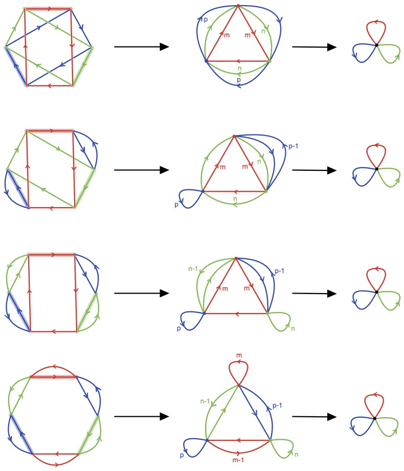
Figure 2. The map $\phi:X_{C}\xrightarrow{\sigma}\overline{X}_{C}\xrightarrow{\iota}X_{A}$ when (1) none, (2) one, (3) two or (4) all of $M,N,P$ are even, respectively. Specifically, $M=2m$ or $2m+1$, $N=2n$ or $2n+1$, and $P=2p$ or $2p+1$. We use the convention where the edge labelled by a number $k$ is a concatenation of $k$ edges of the given color. The thickened edges in $X_{C}$ are the ones that get collapsed to a vertex in $\overline{X}_{C}$

Theorem 5.2 ([Jan22b, Prop 2.8]).

Let $G_{MNP}$ be an Artin group where $M,N\geq 4$ and $P=2$.

• If at least one of $M,N$ is odd, then $G_{MNP}=A*_{C}B$ where $A\simeq F_{2}$, $B\simeq F_{3}$ and $C\simeq F_{5}$, and $[B:C]=2$. The map $C\to A$ is induced by the map $\phi:X_{C}\to X_{A}$ pictured in Figure 3, and the map $C\to B$ is induced by the quotient of the graph $X_{C}$ by a $\pi$ rotation.

  

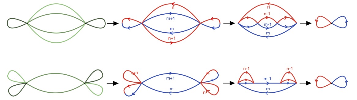
  Figure 3. The map $\phi:X_{C}\xrightarrow{id}X_{C}\xrightarrow{\sigma}\overline{X}_{C}\xrightarrow{\iota}X_{A}$ when $P=2$, $M=2m+1\geq 5$, and (top) $N=2n+1\geq 5$, (bottom) $N=2n\geq 4$, respectively. The use of colors in the leftmost graphs represents the $\pi$-rotation of $X_{C}$.

• If both $M,N$ are even then $G_{MNP}=A*_{B}$ where $A\simeq F_{2}$, $B\simeq F_{3}$. The two maps $B\to A$ are induced by the maps $\phi_{1},\phi_{2}:X_{B}\to X_{A}$ pictured in Figure 4.

  

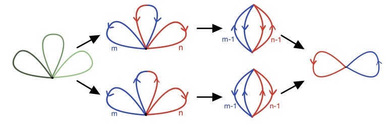
  Figure 4. The maps $\phi_{i}:X_{B}\xrightarrow{id}X_{B}\xrightarrow{\sigma}\overline{X}_{B}\xrightarrow{\iota}X_{A}$ for $i=1,2$, when $M=2m\geq 4$, $N=2n\geq 4$, and $P=2$.

Here is a precise statement of the main theorem of this paper (Theorem 1.1).

Theorem 5.3.

Let $G_{MNP}$ be a triangle Artin group where $M\leq N\leq P$ and either $M>2$, or $N>3$. Then $G_{MNP}$ has finite stature with respect to $\{A\}$, where $A$ is as described in Theorem 5.1 or Theorem 5.2 respectively. All finitely generated subgroups of $A$ are separable in $G_{MNP}$, and in particular $G_{MNP}$ is residually finite.

In subsections 5.4, 5.5, 5.6 and 5.7 we will prove groups $G_{MNP}$ as above have finite stature with respect to $\{A\}$ by analyzing various cases (see Proposition 5.11, Corollary 5.13, Corollary 5.19, and Corollary 5.23). The separability of finitely generated subgroups of $A$ is a consequence of [HW19a, Thm 1.3].

5.2. Some facts about the splittings of Artin groups

We start with some facts that will be used in the next sections. We first focus on the cases where $G_{MNP}$ splits as $A*_{C}B$. Let $\beta:X_{C}\to X_{C}$ be the $\pi$-rotation, as in Theorem 5.1 or Theorem 5.2 respectively. A choice of a path between $x\in X_{C}$ and $\beta(x)\in X_{C}$ determines an element $b\in B-C$, such that the induced homomorphism $C\to C$ is the conjugation by $b$. Figure 2 and Figure 3 illustrate the factorization $\phi=\iota\circ\sigma$ from Proposition 2.2. We denote $\sigma(X_{C})=\overline{X}_{C}$.

We will also extend the definition of $\sigma$ to any precover of $X_{C}$ (and abuse the notation) in the following way. Given a precover $Y\to X_{C}$, let $\overline{Y}\to\overline{X}_{C}$ be a precover, and let $\sigma:Y\to\overline{Y}$ be a composition of edge-subdivisions, Stallings’ folds, and edge-collapses, which locally coincides with $\sigma:X_{C}\to\overline{X}_{C}$. In particular, the following diagram commutes.

We note the following.

Lemma 5.4.

The map $\sigma:Y\to\overline{Y}$ is a homotopy equivalence for every precover $Y\to X_{C}$.

For each subgroup $H\subseteq C$ there is a one-to-one correspondence between the core $Y\to X_{C}$ of $H$ with respect to $X_{C}$ and the core $\overline{Y}\to\overline{X}_{C}$ of $H$ with respect to $\overline{X}_{C}$, where $\overline{Y}=\sigma(Y)$ as above.

Proof.

The map $\sigma:X_{C}\to\overline{X}_{C}$ is obtained as a sequence of edge-subdivisions and edge-collapses of the edges. By analyzing each of the cases in Figure 2 and Figure 3, we note that we never collapse a loop. Thus, by discussion in Section 2, $\sigma:X_{C}\to\overline{X}_{C}$ is a homotopy equivalence. Similarly, any induced map $Y\to\overline{Y}$ is also obtained as a sequence of edge-subdivisions and edge-collapses of the edges that are not loops, and hence $\sigma:Y\to\overline{Y}$ is a homotopy equivalence. By construction $Y\to X_{C}$ is the core of some subgroup $H\subseteq\pi_{(}X_{C})$ with respect to $X_{C}$ if and only if $\overline{Y}\to\overline{X}_{C}$ is the core of $H$ with respect to $\overline{X}_{C}$. ∎

We will use the notation $\sigma^{-1}(\overline{Y})$ to denote $Y$ such $\overline{Y}=\sigma(Y)$.

Lemma 5.5.

Let $H\subseteq C$ be a subgroup, and let $Y\to X_{C}$ be its core with respect to $X_{C}$. Then $Y\to X_{C}\xrightarrow{\beta}X_{C}$ is the core of $H^{b}\subseteq C$

Proof.

Indeed, $Y\to X_{C}$ induces the inclusion $H\to C$ and $X_{C}\xrightarrow{\beta}X_{C}$ induces the conjugation by $b$. ∎

The following lemma will allow us to apply Proposition 3.3.

Lemma 5.6.

Let $T$ be the Bass-Serre tree of the splitting $G_{MNP}=A*_{C}B$, and $\rho$ be a finite path in $T$. The stabilizer $\operatorname{Stab}(\rho)$ of a path $\rho$ of length $2\ell$ between a pair of $A$-vertices, is conjugate to a subgroup of $C$, represented by a precover $\overline{Y}_{\ell}\to\overline{X}_{C}$, where the corresponding $Y_{\ell}$ is defined recursively:

• $Y_{1}=X_{C}$,

• $Y_{\ell}=\sigma^{-1}(\overline{Y}_{\ell-1}\otimes_{X_{A}}\overline{Y}_{\ell-1})$ for even $\ell$,

• $Y_{\ell}=\sigma^{-1}(\overline{Y}_{\ell-1}\otimes_{X_{A}}\sigma\cdot\beta(Y_{\ell-1}))$ for odd $\ell$

The map $\overline{Y}_{\ell-1}\to X_{A}$ in the recursive definition above is obtained by composing the map $\overline{Y}_{\ell-1}\to\overline{X}_{C}$ with the map $\overline{X}_{C}\to X_{A}$.

Proof.

Let $\rho$ be a path of length $2\ell$. By Lemma 4.2, $\operatorname{Stab}(\rho)$ is conjugate to a group $K_{\ell}$ defined recursively as

• $K_{1}=C$,

• if $\ell$ is even, then $K_{\ell}=K_{\ell-1}\cap(K^{\prime}_{\ell-1})^{a_{1}}$.

• if $\ell$ is odd, then $K_{\ell}=K_{\ell-1}\cap(K^{\prime}_{\ell-1})^{b}$,

Clearly, $Y_{1}=X_{C}\to X_{C}$ is the core of $L_{1}=C$ with respect to $X_{C}$. For even $\ell$, $K_{\ell}=K_{\ell-1}\cap(K^{\prime}_{\ell-1})^{a}$, so by Lemma 2.4 the core of $K_{\ell}$ with respect to $\overline{X}_{C}$ is $\overline{Y}_{\ell-1}\otimes_{X_{A}}\overline{Y}_{\ell-1}$, and by Lemma 5.4 the core of $K_{\ell}$ with respect to $X_{C}$ is $\sigma^{-1}(\overline{Y}_{\ell-1}\otimes_{X_{A}}\overline{Y}_{\ell-1})$. For odd $\ell$, $K_{\ell}=K_{\ell-1}\cap(K^{\prime}_{\ell-1})^{b}$, so by Lemma 2.4 and Lemma 5.5 the core $K_{\ell}$ with respect to $\overline{X}_{C}$ is $\overline{Y}_{\ell-1}\otimes_{X_{A}}\sigma\cdot\beta(Y_{\ell-1})$, and by Lemma 5.4 the core of $K_{\ell}$ with respect to $X_{C}$ is $\sigma^{-1}(\overline{Y}_{\ell-1}\otimes_{X_{A}}\sigma\cdot\beta(Y_{\ell-1}))$. ∎

Again, we emphasize that graphs $Y_{\ell}$ are not uniquely determined, as they are associated to non-unique $K_{\ell}$’s. Since a sequence of group $C=K_{1}\supseteq K_{2}\supseteq K_{3}\supseteq\dots$ form a descending chain, we have a corresponding sequence of precovers $\dots\xrightarrow{}Y_{3}\to Y_{2}\to Y_{1}=X_{C}$.

Lemma 5.7.

Suppose that there are only finitely many isomorphism types of graphs $Y_{\ell}$ for any $\ell\geq 1$. Then $G_{MNP}$ has finite stature with respect to $\{A\}$.

In particular if there exists $k\geq 1$ such that every map $\overline{Y}_{k+2}\to\overline{Y}_{k}$ is an embedding of a subgraph, then $G_{MNP}$ has finite stature with respect to $\{A\}$.

Proof.

We first prove the first statement. Let $T$ be the Bass-Serre tree $T$ of $G_{MNP}=A*_{C}B$, and $\tilde{v}\in T$ be a vertex whose stabilizer is $A$. By Lemma 5.6 and Lemma 4.2 there are finitely many conjugacy classes of $\operatorname{Stab}(\rho)$ (viewed as subgroups of $A$) for finite paths $\rho$ in $T$ joining two $A$-vertices and passing through $\tilde{v}$. Since every finite path passing through $\tilde{v}$ is contained in such a path joining two $A$-vertices, we conclude that the assumptions of Proposition 3.3 are satisfied. We deduce that $G_{MNP}$ has finite stature with respect to $\{A\}$.

Now let $k\geq 1$ such that $Y_{k+2}\to Y_{k}$ is an inclusion. Since $Y_{k+2}$ is obtained from $Y_{k}$ in two steps as described in Lemma 5.6, we deduce that $Y_{k+2(i+1)}\to Y_{k+2i}$ is an inclusion for each $i\geq 0$. In particular, there can only be finitely many color-preserving isomorphism types of graphs $Y_{k+2i}$ since $Y_{k}$, as a finite graph, has only finitely many subgraphs. Using the formula for $Y_{k+2i+1}$ from Lemma 5.6 we deduce that there are finitely many isomorphism types of graphs $Y_{\ell}$ for any $\ell\geq 1$. The conclusion follows from the first part of the lemma. ∎

5.3. Monochrome cycle preserving structure of splitting of Artin groups

Proposition 5.8.

Let $G_{MNP}$ be an Artin group where $M\leq N\leq P$ and either $M>2$ or $N>3$. Then $G_{MNP}$ has a subgroup $G^{\prime}$ of index at most $2$ that is the fundamental group of a monochrome cycles preserivng graph of graphs $X_{A}\xleftarrow{\phi}X_{C}\xrightarrow{\beta\cdot\phi}X_{A}$.

Proof.

Let $G_{MNP}=A*_{C}B$ as in Theorem 5.1 or Theorem 5.2. Then $G_{MNP}$ has an index $2$ subgroup $G^{\prime}$ which splits as $A*_{C}A$. The associated graph of graphs has two vertices with each vertex graph being a copy of $X_{A}$, and one edge graph $X_{C}$. We choose the coloring of $c_{A}:X_{A}\to\{\text{red},\text{green},\text{blue}\}$, where each loop has distinct color, as in Figure 2 or Figure 3. Those figure also show how the coloring is $c_{C}:X_{C}\to\{\text{red},\text{green},\text{blue}\}$ is defined. The two maps $X_{C}\to X_{A}$ differ by precomposing one with the automorphism $\beta$ of $X_{C}$. In particular, both maps $X_{C}\to X_{A}$ are color-preserving, and the preimage of each color in $X_{C}$ is a union of disjoint embedded cycles. Moreover, the maps $X_{C}\to X_{A}$ both factor through $\overline{X}_{C}$, and in particular, both maps restricted to each cycle factors through a cycle of length $Q$ if $Q$ is odd, and $Q/2$ is $Q$ is even, for $Q=M,N,P$ respectively. Thus the graphs of graphs $X_{A}\xleftarrow{\phi}X_{C}\xrightarrow{\beta\cdot\phi}X_{A}$ is monochrome cycles preserving. ∎

Every finite path $\rho$ in the Bass-Serre tree of $G_{MNP}=A*_{C}B$ joining a pair of $A$-vertices can be also thought of as a path in the Bass-Serre tree of the index $2$ subgroup $G^{\prime}=A*_{C}A$ of $G_{MNP}$. By Proposition 5.8 above and Lemma 4.4, for the precover $Y_{\rho}\to X_{A}$ of $\operatorname{Stab}(\rho)$ the associated graph $\overline{Y}_{\rho}$ is a union of monochrome cycles, where each cycle of color $i$ has length $\ell_{i}$. We can denote the the $2$- complex obtained from $Y_{\rho}$ by attaching $2$-cells whose boundaries have color $i$ and length $\ell_{i}$ by $\widetriangle Y_{\rho}$, as in Section 4.2.

Notation 5.9.

We now switch to the use of notation of Lemma 5.6, where the graph $Y_{\rho}$ is denoted by $Y_{\ell}$ where $2\ell=|\rho|$, and the associated $K_{\ell}$ is the stabilizer $\operatorname{Stab}(\rho)$. We will also write $\widetriangle Y_{\ell}$ for $\widetriangle Y_{\rho}$. Once again, we remind that $Y_{\ell}$, $K_{\ell}$ depend not only on $\ell$, but also the choice of parameters $a_{i},d_{i}$ in their definition, which are equivalent to the choice of $\rho$.

Lemma 5.10.

If for some $\ell\geq 1$ a complex $\widetriangle Y_{\ell}$ is simply connected, then for every $\overline{Y}_{\ell+2}$, the precover $\overline{Y}_{\ell+2}\to\overline{Y}_{\ell}$ is an embedding of a subgraph. In particular, if there exists $\ell\geq 1$ such that every $\widetriangle Y_{\ell}$ is simply connected, then $G_{MNP}$ has finite stature with respect to $\{A\}$.

Proof.

The first statement follows directly from Lemma 4.5. Since there are only finitely many color-preserving isomorphism types of $\overline{Y}_{k}$, there are also only finitely many color-preserving isomorphism types of their subgraphs. Thus if all $Y_{k}$ are simply-connected, there are only finitely many color-preserving isomorphism types of graphs that $\overline{Y}_{\rho}$ might have. It follows that there are only finitely many conjugacy classes of the groups of the form $G_{\tilde{v}}\cap\operatorname{Stab}(\rho)$. By Proposition 3.3 $G^{\prime}$ has finite stature with respect to both copies of $A$. By Proposition 3.4 $G_{MNP}$ also has finite stature with respect to $\{A\}$. ∎

In the next subsections we apply Lemma 5.7 or Lemma 5.10 to prove that all the large type triangle Artin group have finite stature. We consider three cases:

1. at least one $M,N,P\geq 3$ is even and $\{M,N,P\}\neq\{2m+1,4,4\}$ for $m\geq 1$,

2. $\{M,N,P\}=\{2m+1,4,4\}$ where $m\geq 1$,

3. all $M,N,P$ are odd and $\geq 3$.

We also consider the case where one of the exponents is $2$, and the other two are both strictly greater than $3$:

1. $\{M,N,P\}$ where $M,N\geq 4$ and $P=2$.

5.4. Case where at least one of $M,N,P\geq 3$ is even and $\{M,N,P\}\neq\{2m+1,4,4\}$

In the next proof, we continue to use Notation 5.9.

Proposition 5.11.

Suppose $M,N,P\geq 3$ and at least one of them is even, but $\{M,N,P\}\neq\{2m+1,4,4\}$. Then $G_{MNP}$ has finite stature with respect to $\{A\}$, where $A$ is as in Theorem 5.1.

Proof.

By Theorem 5.1 in all the cases listed in the statement, $G_{MNP}$ splits as an amalgamated product $A*_{C}B$ of finite rank free groups where $[B:C]=2$, which by Proposition 5.8 is virtually the fundamental group of a monochrome cycles preserving graph of graphs. By [Jan22a, Lem 5.2, 5.3, 5.4] (see also [Jan22a, Rem 5.5]) $\widetriangle Y_{2}$ is simply-connected, where $Y_{2}\to X_{C}$ if the core of $C\cap C^{g}$ with respect to $X_{C}$, as in Lemma 5.6. By Lemma 5.10 $G_{MNP}$ has finite stature with respect to $\{A\}$. ∎

We note that the residual finiteness of the Artin groups considered above was also proven in [Jan22a].

5.5. Case where $\{M,N,P\}=\{2m+1,4,4\}$

We continue to use Notation 5.9.

Lemma 5.12.

Let $\{M,N,P\}=\{2m+1,4,4\}$. Every graph $\overline{Y}_{2}$ is either the left graph in Figure 5, or has simply connected $\widetriangle Y_{2}$. Every graph $\overline{Y}_{3}$ is either the right graph in Figure 5, or has simply connected $\widetriangle Y_{3}$. The map $\overline{Y}_{4}\to\overline{Y}_{2}$ is always an embedding of a subgraph.

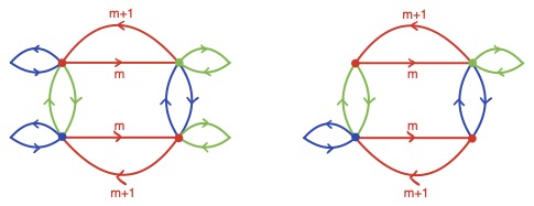
Figure 5. $(M,N,P)=(2m+1,4,4)$. The graph on the left is the fiber product $\overline{Y}_{2}=\overline{X}_{C}\otimes_{X_{A}}\overline{X}_{C}$. The graph on the right is $\sigma\beta(Y_{2})\otimes_{X_{A}}\overline{Y}_{2}$.

Proof.

By Theorem 5.1 in all the cases listed in the statement, $G_{MNP}$ splits as an amalgamated product $A*_{C}B$ of finite rank free groups where $[B:C]=2$, which by Proposition 5.8 is virtually the fundamental group of a monochrome cycles preserving graph of graphs.

By Lemma 5.6, $\overline{Y}_{2}$ is computed as a connected component of the fiber product $\overline{Y}_{1}\otimes_{X_{A}}\overline{Y}_{1}$, which has been done in [Jan22a, Lem 5.1]. If $\widetriangle Y_{2}$ is simply-connected, then $\overline{Y}_{4}\to\overline{Y}_{2}$ is an embedding of a subgraph for every $Y_{4}$, by Lemma 5.10.

In the case where $\widetriangle Y_{2}$ is not simply connected, the resulting map $\overline{Y}_{2}\to\overline{X}_{C}$ is illustrated as the first vertical arrow in Figure 6. Lemma 5.4 ensures that $Y_{2}\to X_{C}$ can be computed, which is done in the second vertical arrow in Figure 6. Then the rest of Figure 6 represent the computation of $\sigma\beta(Y_{2})\to\overline{X}_{C}$. Finally, by Lemma 5.6, $\overline{Y}_{3}$ is computed as the fiber product $\sigma\beta(Y_{2})\otimes_{X_{A}}\overline{Y}_{2}$, i.e. the fiber product of the left top and the right top graphs in Figure 6. We deduce that $\overline{Y}_{3}$ either has simply connected $\widetriangle Y_{3}$, or it is the right graph in Figure 5.

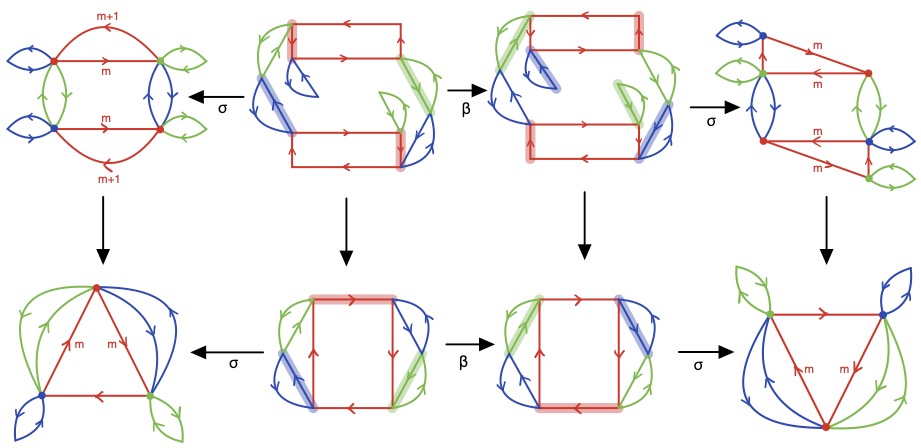
Figure 6. $(M,N,P)=(2m+1,4,4)$. The vertical arrows are respectively: $\overline{Y}_{2}\to\overline{X}_{C}$, $Y_{2}\to X_{C}$, $\beta(Y_{2})\to X_{C}$, and $\sigma\cdot\beta(Y_{2})\to\overline{X}_{C}$.

If $\widetriangle Y_{3}$ is simply-connected, then so is $\widetriangle Y_{4}$ and $\overline{Y}_{4}\to\overline{Y}_{2}$ is an embedding of a subgraph, as required. Otherwise, $\overline{Y}_{4}$ is a connected component of $\overline{Y}_{3}\otimes_{X_{A}}\overline{Y}_{3}$ by Lemma 5.6. Note that each connected component $\overline{Y}_{4}$ is either equal to $\overline{Y}_{3}$, or has simply connected $\widetriangle Y_{4}$, and in particular, the map $\overline{Y}_{4}\to\overline{Y}_{2}$ is an embedding of a subgraph. ∎

Combining Lemma 5.12 and Lemma 5.7 yields the following.

Corollary 5.13.

The Artin group $G_{MNP}$ where $M=2m+1\geq 3$ and $N=P=4$ has finite stature with respect to $\{A\}$, where $A$ is as described in Theorem 5.1.

5.6. Case where $M,N,P\geq 3$ are all odd

First consider the case where $M=N=P=3$.

Proposition 5.14.

Let $(M,N,P)=(3,3,3)$, and let $T$ be the Bass-Serre tree of the splitting $G_{333}=A*_{C}B$. Then for every path $\rho$ in $T$, $\operatorname{Stab}(\rho)=C$.

Proof.

Indeed, in this case $C$ is normal in both $A$ and $B$, so all $G_{333}$-conjugates of $C$ are equal $C$. This proves that all edge stabilizers in the action of $G_{333}$ on $T$ are equal $C$. ∎

For the remaining cases, we will apply Lemma 5.7 to deduce that $G_{MNP}$ has finite stature with respect to $\{A\}$, similarly as in Section 5.5 We now consider the case where $M,N,P$ are all at least $5$. We continue to use Notation 5.9.

Lemma 5.15.

Let $M,N,P\geq 5$ be all odd. Every graph $\overline{Y}_{2}$ is either the left graph in Figure 7, or has simply connected $\widetriangle Y_{2}$. Also, every graph $\overline{Y}_{3}$ is either the right graph in Figure 7, or has simply connected $\widetriangle Y_{3}$. The map $\overline{Y}_{4}\to\overline{Y}_{2}$ is always an embedding of a subgraph.

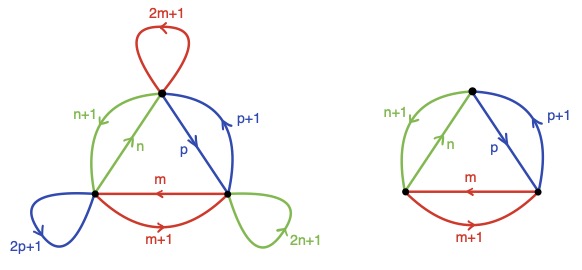
Figure 7. $(M,N,P)=(2m+1,2n+1,2p+1)$. The graph on the left is the fiber product $\overline{Y}_{2}=\overline{X}_{C}\otimes_{X_{A}}\overline{X}_{C}$. The graph on the right is $\sigma\beta(Y_{2})\otimes_{X_{A}}\overline{Y}_{2}$.

Proof.

We write $M=2m+1$, $N=2n+1$, and $P=2p+1$. The first part of the lemma was proven in [Jan22a, Lem 5.1]. In order to prove the second part we start with computing $\sigma\beta(Y_{2})$, which is illustrated in Figure 8.

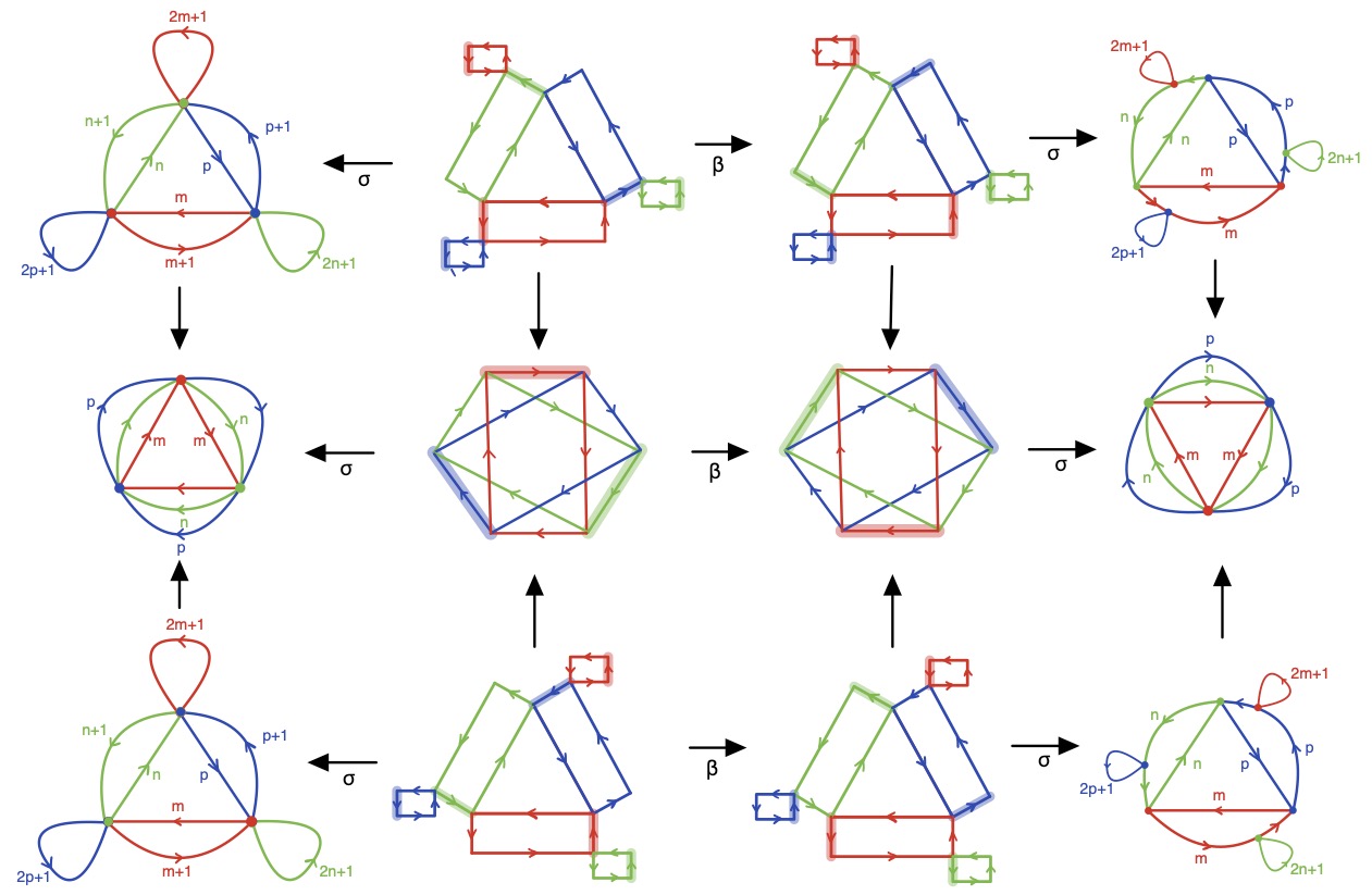
Figure 8. $(M,N,P)=(2m+1,2n+1,2p+1)$. Each of the two rows of vertical arrows corresponds to respectively: $\overline{Y}_{2}\to\overline{X}_{C}$, $Y_{2}\to X_{C}$, $\beta(Y_{2})\to X_{C}$, and $\sigma\beta(Y_{2})\to\overline{X}_{C}$.

We note that there are two connected components $Y_{2}$ of the fiber product $\overline{X}_{C}\otimes_{X_{A}}\overline{X}_{C}$ for which $\widetriangle Y_{3}$ is not simply connected. They are both color-preserving isomorphic to the left graph in Figure 7, but their maps to $X_{C}$ are different. The first column of Figure 8 shows the two precovers $\overline{Y}_{2}\to\overline{X}_{C}$ (they are determined by the coloring of the vertices). For each $Y_{2}$, we compute $\sigma\beta(Y_{2})$, in a similar manner as in Lemma 5.12, see the rest of Figure 8. In each case, we deduce that each connected component $\overline{Y}_{3}$ of $\overline{Y}_{2}\otimes_{X_{A}}\sigma\beta(Y_{2})$ either has simply connected $\widetriangle Y_{3}$, or it is the right graph in Figure 7. In either case, we every map $\overline{Y}_{4}\to\overline{Y}_{2}$ is an embedding of a subgraph by a reasoning similar to one in Lemma 5.12. ∎

We now move to the case where one or two of $M,N,P$ are equal to $3$. Unlike in the previous case, the computation of the fiber product $\overline{X}_{C}\otimes_{X_{A}}\overline{X}_{C}$ in such cases was not included in [Jan22a]. We start with that computation.

Lemma 5.16.

Suppose one or two of $M,N,P$ are equal to $3$. Every connected component $Y_{2}$ of $\overline{X}_{C}\otimes_{X_{A}}\overline{X}_{C}$ either has simply connected $\widetriangle Y_{2}$ or is

• the left graph in Figure 9, when $M=3$ and $N,P\geq 5$,

• the right graph in Figure 9, when $M=N=3$ and $P\geq 5$,

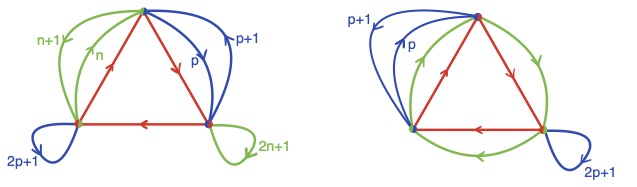
Figure 9. $(M,N,P)=(2m+1,2n+1,2p+1)$. A connected component of $\overline{X}_{C}\otimes_{X_{A}}\overline{X}_{C}$, when $M=3$ and $N,P\geq 5$ (left), $M=N=3$ and $P=\geq 5$ (right).

Proof.

This is a direct computation. We remind that the graph $\overline{X}_{C}$ is the middle graph in the first row of Figure 2. In Figure 9 we bi-colored the vertices of the graphs (i.e. colored with a pair of colors) to make it easier for the reader to verify the computation. ∎

Now our goal is to show that $\overline{Y}_{\ell+2}\to\overline{Y}_{\ell}$ is an embedding of a subgraph for some $\ell$, so we can apply Lemma 5.7. The case where exactly one of $M,N,P$ is equal $3$ is considered first.

Lemma 5.17.

Let $N,P\geq 5$ be odd, and $M=3$. Every $\overline{Y}_{3}$ is either a single monochrome cycle or one of the graphs in Figure 10, and in particular has simply connected $\widetriangle Y_{3}$.

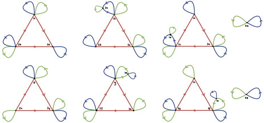
Figure 10. $(M,N,P)=(3,2n+1,2p+1)$. All the connected components of $\overline{Y}_{2}\otimes_{X_{A}}\sigma\beta(Y_{2})$ is either a cycle or one of the graphs pictured above. Each green loop has length $2n+1$, and each blue loop has length $2p+1$. The top row here corresponds to $\sigma\beta(Y_{2})$ in the top row of Figure 11, and the bottom row here corresponds to $\sigma\beta(Y_{2})$ in the bottom row of Figure 11. We include labels of vertices as $1c$, $2b$ etc, where the number corresponds to a vertex of $\overline{Y}_{2}$ and the letter corresponds to a vertex of $\sigma\beta(Y_{2})$.

Proof.

We write $N=2n+1$ and $P=2p+1$. By Lemma 5.16, every $Y_{2}$ either has simply connected $\widetriangle Y_{2}$ or is the left graph in Figure 9. There are two components of $\overline{X}_{C}\otimes_{X_{A}}\overline{X}_{C}$ color-preserving isomorphic to the left graph in Figure 9. We compute $\sigma\beta(Y_{2})$ similarly as in Lemma 5.15 and Lemma 5.17. This is illustrated in Figure 11.

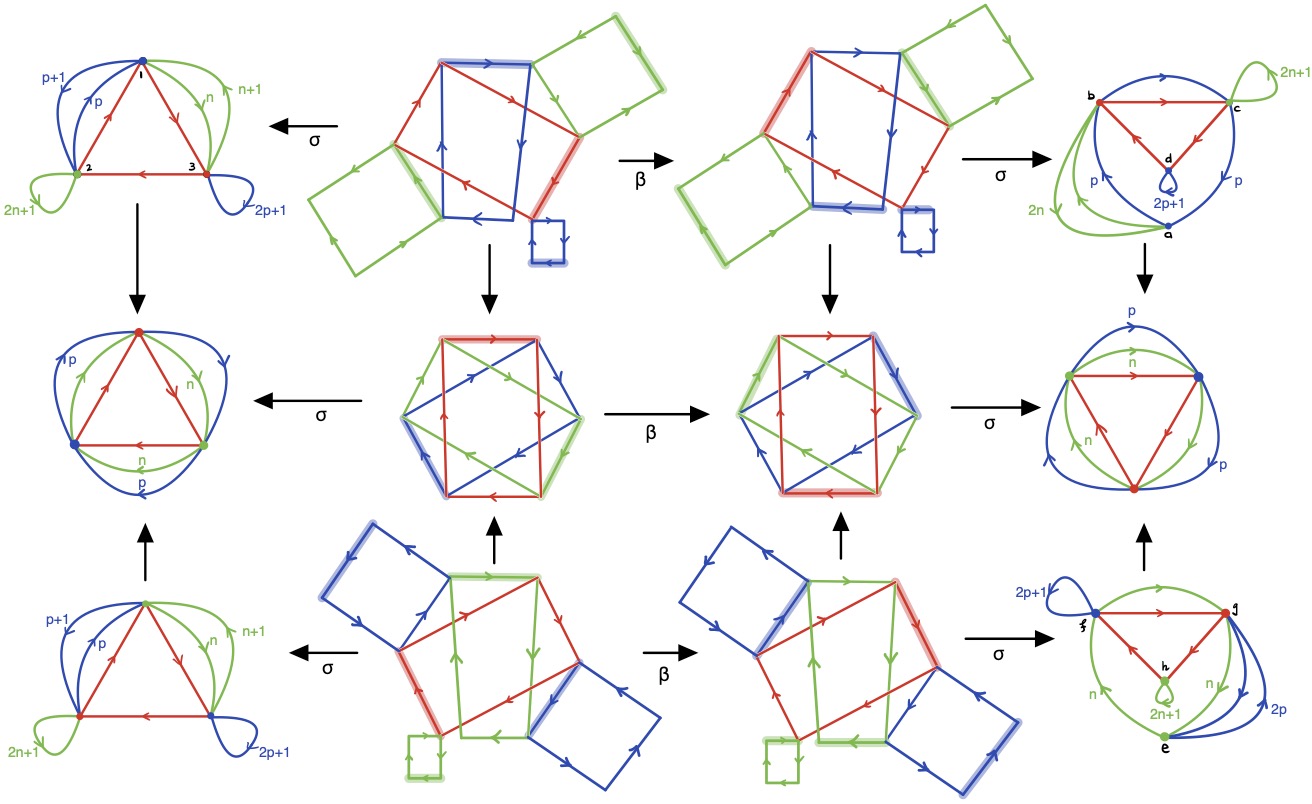
Figure 11. $(M,N,P)=(3,2n+1,2p+1)$. Each of the two rows of vertical arrows corresponds to respectively: $\overline{Y}_{2}\to\overline{X}_{C}$, $Y_{2}\to X_{C}$, $\beta(Y_{2})\to X_{C}$, and $\sigma\beta(Y_{2})\to\overline{X}_{C}$.

Next, for each of the two choices of $\sigma\beta(Y_{2})$ (as illustrated in Figure 9) we compute the fiber product $\overline{Y}_{2}\otimes\sigma\beta(Y_{2})$. The labelling of the vertices in the top left, top right and the bottom right graph in Figure 9, will help the reader to verify that all the connected components of those fiber products are either pictured in Figure 10 or consist of a single monochrome cycle. Finally, we conclude that for every $\overline{Y}_{3}$, the complex $\widetriangle Y_{3}$ is simply connected. ∎

In the remaining case exactly two of $M,N,P$ are equal $3$.

Lemma 5.18.

Let $P\geq 5$ be odd, and $M=N=3$. Every $\overline{Y}_{3}$ either has simply connected $\widetriangle Y_{3}$, or is one of the graphs in Figure 12.

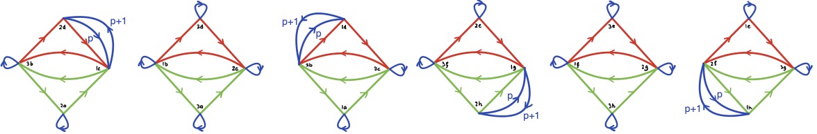
Figure 12. $(M,N,P)=(3,3,2p+1)$. Each unlabelled blue loop has length $2p+1$.

Moreover, the map $\overline{Y}_{5}\to\overline{Y}_{3}$ is always an embedding of a subgraph.

Proof.

We write $P=2p+1$. By Lemma 5.16, every $Y_{2}$ either has simply connected $\widetriangle Y_{2}$ or is color-preserving isomorphic to the right graph in Figure 9.

We compute $\sigma\beta(Y_{2})$ similarly as in Lemma 5.17. This is illustrated in Figure 13.

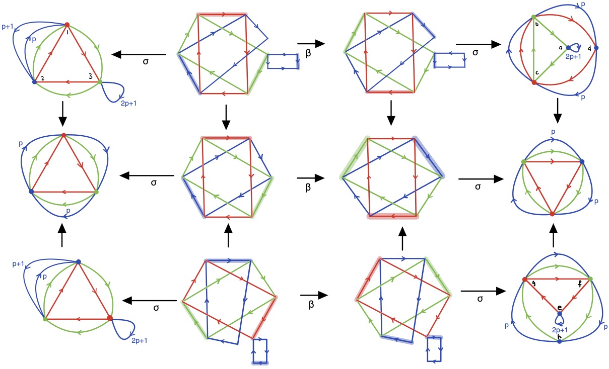
Figure 13. $(M,N,P)=(3,3,2p+1)$. Each of the two rows of vertical arrows corresponds to respectively: $\overline{Y}_{2}\to\overline{X}_{C}$, $Y_{2}\to X_{C}$, $\beta(Y_{2})\to X_{C}$, and $\sigma\beta(Y_{2})\to\overline{X}_{C}$.

Once again, for each of the two choices of $\sigma\beta(Y_{2})$ we compute the fiber product $\overline{Y}_{2}\otimes\sigma\beta(Y_{2})$. As a result we obtain that $\overline{Y}_{3}$ is either a monochrome (blue) cycle, or it is color-preserving isomorphic to one of the graphs in Figure 12.

We now note that the collection of graphs in Figure 12:

• has the property that the fiber product of any two graphs is a subgraph of one of the graphs in the collection, and

• is invariant under $\beta$, see Figure 14.

The first fact implies that every $\overline{Y}_{4}$ is a subgraph of some $\overline{Y}_{3}$. The second fact implies that this is also the case for $\overline{Y}_{5}$. In particular, every $\overline{Y}_{5}\to\overline{Y}_{3}$ is an embedding.

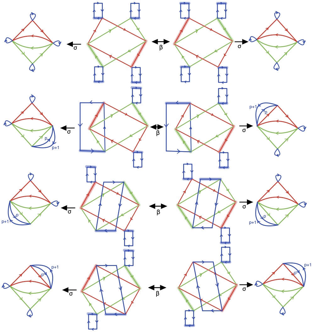
Figure 14. Each unlabelled blue loop has length $2p+1$

∎

We now summarize what we have proven in this subsection.

Corollary 5.19.

The Artin group $G_{MNP}$ where $M,N,P\geq 3$ are odd has finite stature with respect to $\{A\}$, where $A$ is as described in Theorem 5.1.

Proof.

When $M=N=P=3$, the statement follows from Proposition 5.14. The case where $M=N=3$, and $P=2p+1\geq 5$ follows from Lemma 5.18 and Lemma 5.7. The case where $M=3$, $N=2n+1\geq 5$, and $P=2p+1\geq 5$ follows from Lemma 5.17 and Lemma 5.7. Finally, the case where $M=2m+1\geq 5$, $N=2n+1\geq 5$, and $P=2p+1\geq 5$ is a consequence of Lemma 5.15 and Lemma 5.7. ∎

We note that the residual finiteness of $G_{333}$ follows from [Squ87]. The residual finiteness of $G_{MNP}$ where $M,N,P\geq 5$ was proven in [Jan22a]. However, the methods of [Jan22a] do not cover the cases where one or two of $M,N,P$ are equal $3$.

5.7. The case where $\{M,N,2\}$ where $M,N\geq 4$

We first focus on the case where $M,N$ are both even. We recall that, unlike in the previous cases, $G_{MNP}$ splits as an HNN-extension $A*_{B}$, as in Theorem 5.2.

Lemma 5.20.

Let $M=2m,N=2n$ and $P=2$. The graphs $\overline{\phi_{1}X_{B}}$ and $\overline{\phi_{2}X_{B}}$ are (unbased) color-preserving isomorphic. In particular, the stabilizer of every finite path in the Bass-Serre tree of the splitting of $G_{MNP}=A*_{B}$ is conjugate to a subgroup of $A$ represented by $\overline{\phi_{1}X_{B}}$ or a wedge of monochrome cycles.

Proof.

The graphs $\overline{\phi_{1}X_{B}}$ and $\overline{\phi_{2}X_{B}}$ are computed in Theorem 5.2, and it is easy to see that the two graphs are color-preserving isomorphic. Every connected component $Y$ of the fiber product $\overline{\phi_{1}X_{B}}\otimes_{X_{A}}\overline{\phi_{1}X_{B}}$ is either color-preserving isomorphic to $\overline{\phi_{1}X_{B}}$ or is a wedge of monochrome cycles. ∎

Next, we consider the cases where at both $M,N$ are odd.

Lemma 5.21.

Let $P=2$ and $M=2m+1,N=2n+1\geq 5$. Every graph $\overline{Y}_{2}$ either is color-preserving isomorphic to the left graph in Figure 15(a) or it is a wedge of monochrome cycles. If $Y$ is the left graph in Figure 15(a), then $\sigma\beta(Y)$ is (unbased) isometric to $Y$. Therefore, every graph $\overline{Y}_{i}$ either one of the two graphs in Figure 15(a), or it is a wedge of monochrome cycles.

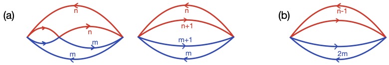
Figure 15. $P=2$. All the graphs $\overline{Y}_{\ell}$ are either wedges of circles, or one of the graphs above, when (a) $M,N\geq 5$ are both odd and $P=2$, and (b) exactly one of $M,N\geq 4$ is odd and $P=2$.

Proof.

The first statement was proven in [Jan22b, Rem 3.5]. The proof of the second statement is illustrated in Figure 16(a). Let $\overline{Y}_{2}$ be the left graph in Figure 15(a). Then every connected component $\overline{Y}_{3}$ of the fiber product $\overline{Y}_{2}\otimes_{X_{A}}\sigma\beta(Y_{2})=\overline{Y}_{2}\otimes_{X_{A}}\overline{Y}_{2}$ is a wedge of monochrome cycles, is isomorphic to $\overline{Y}_{2}$ or to the right graph in Figure 15(a). We also note that if $Y$ is the right graph in Figure 15(b), then $\sigma\beta(Y)$ is isometric to $Y$. We conclude that every graph $\overline{Y}_{\ell}$ either one of the two graphs in Figure 15(a), or it is a wedge of monochrome cycles.

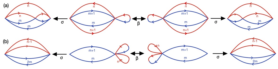
Figure 16. $(M,N,2)=(2m+1,N,2)$. In case (a) $N=2n+1$, and in case (b) $N=2n$. If $\overline{Y}$ is the rightmost graphs, then it is isometric to $\sigma\beta(Y)$.

∎

Finally, we consider the cases where exactly one of $M,N$ is odd.

Lemma 5.22.

Let $P=2$, $M=2m+1\geq 5$, and $N=2n\geq 4$. Every graph $\overline{Y}_{2}$ either is isometric to the graph in Figure 15(b) or it is a wedge of monochrome cycles. If $Y$ is the graph in Figure 15(b), then $\sigma\beta(Y)$ is (unbased) isometric to $Y$. Therefore, every graph $\overline{Y}_{i}$ either one of the graph in Figure 15(b), or it is a wedge of monochrome cycles.

Proof.

The first statement was proven in [Jan22b, Prop 3.4]. The proof of the second statement is illustrated in Figure 16(b). Let $Y$ denote the graph in Figure 16(b). Every connected component of the fiber product $Y\otimes_{X_{A}}Y$ is either isometric to $Y$ or it is a wedge of monochrome cycles. ∎

Corollary 5.23.

The Artin group $G_{MN2}$ where $M,N\geq 4$ has finite stature with respect to $\{A\}$, where $A$ is as described in Theorem 5.1.

Proof.

All the cases can be deduced from Lemma 5.7 together with

• Lemma 5.20 when $M,N$ are both even;

• Lemma 5.22 when exactly one of $M,N$ is odd;

• Lemma 5.21 when both $M,N$ are odd.∎

Residual finiteness of $G_{MN2}$ where at least one of $M,N$ is even was proven in [Jan22b], but the case of both $M,N$ odd is a new result.

5.8. Triangle Artin groups with label $\infty$

Note that all of the above proofs are valid if any of the labels $M,N,P$ are equal to $\infty$.

References

- [BGJP18] Rubén Blasco-García, Arye Juhász, and Luis Paris. Note on the residual finiteness of Artin groups. J. Group Theory, 21(3):531–537, 2018.
- [BGMPP19] Rubén Blasco-García, Conchita Martínez-Pérez, and Luis Paris. Poly-freeness of even Artin groups of FC type. Groups Geom. Dyn., 13(1):309–325, 2019.
- [Big01] Stephen J. Bigelow. Braid groups are linear. J. Amer. Math. Soc., 14(2):471–486 (electronic), 2001.
- [CW02] Arjeh M. Cohen and David B. Wales. Linearity of Artin groups of finite type. Israel J. Math., 131:101–123, 2002.
- [Dig03] François Digne. On the linearity of Artin braid groups. J. Algebra, 268(1):39–57, 2003.
- [GMRS98] Rita Gitik, Mahan Mitra, Eliyahu Rips, and Michah Sageev. Widths of subgroups. Trans. Amer. Math. Soc., 350(1):321–329, 1998.
- [Hae21] Thomas Haettel. Virtually cocompactly cubulated Artin-Tits groups. Int. Math. Res. Not. IMRN, (4):2919–2961, 2021.
- [HJP16] Jingyin Huang, Kasia Jankiewicz, and Piotr Przytycki. Cocompactly cubulated 2-dimensional Artin groups. Comment. Math. Helv., 91(3):519–542, 2016.
- [HW19a] Jingyin Huang and Daniel T. Wise. Stature and separability in graphs of groups, 2019.
- [HW19b] Jingyin Huang and Daniel T. Wise. Virtual specialness of certain graphs of special cube complexes. Math. Ann, pages 1–27, 2019. To appear.
- [Jan22a] Kasia Jankiewicz. Residual finiteness of certain 2-dimensional Artin groups. Adv. Math., 405:Paper No. 108487, 2022.
- [Jan22b] Kasia Jankiewicz. Splittings of triangle Artin groups as graphs of finite rank free groups. Groups Geom. Dyn., pages 1–14, 2022. To appear.
- [JS23] Kasia Jankiewicz and Kevin Schreve. Profinite aspects of algebraically clean graphs of groups. In Preparation., 2023.
- [Kra02] Daan Krammer. Braid groups are linear. Ann. of Math. (2), 155(1):131–156, 2002.
- [Liu13] Yi Liu. Virtual cubulation of nonpositively curved graph manifolds. J. Topol., 6(4):793–822, 2013.
- [PW14] Piotr Przytycki and Daniel T. Wise. Graph manifolds with boundary are virtually special. J. Topol., 7(2):419–435, 2014.
- [Squ87] Craig C. Squier. On certain -generator Artin groups. Trans. Amer. Math. Soc., 302(1):117–124, 1987.
- [Sta83] John R. Stallings. Topology of finite graphs. Invent. Math., 71(3):551–565, 1983.
- [Wis02] Daniel T. Wise. The residual finiteness of negatively curved polygons of finite groups. Invent. Math., 149(3):579–617, 2002.