Robust graph-based methods for overcoming the curse of dimensionality

Abstract

Graph-based two-sample tests and graph-based change-point detection that utilize a similarity graph provide a powerful tool for analyzing high-dimensional and non-Euclidean data as these methods do not impose distributional assumptions on data and have good performance across various scenarios. Current graph-based tests that deliver efficacy across a broad spectrum of alternatives typically reply on the $K$-nearest neighbor graph or the $K$-minimum spanning tree. However, these graphs can be vulnerable for high-dimensional data due to the curse of dimensionality. To mitigate this issue, we propose to use a robust graph that is considerably less influenced by the curse of dimensionality. We also establish a theoretical foundation for graph-based methods utilizing this proposed robust graph and demonstrate its consistency under fixed alternatives for both low-dimensional and high-dimensional data.

Keywords: edge-count two-sample tests, curse of dimensionality, permutation null distribution

1 Introduction

Two-sample hypothesis testing is a fundamental task in statistics and have been extensively explored. Nowadays, the growing prevalence of complex data in various fields like genomics, finance, and social networks has led to a rising demand for methods capable of handling high-dimensional and non-Euclidean data [Bullmore and Sporns, 2009, Koboldt et al., 2012, Feigenson et al., 2014, Beckmann et al., 2021]. Parametric approaches are limited in many ways when dealing with a large number of features and various data types as they are often confined by particular parametric families.

In the nonparametric domain, two-sample testing has numerous advancements over the years. Friedman and Rafsky [1979] proposed the first practical method that can be applied to data in an arbitrary dimension. This method (we call it the original edge-count test (OET) for easy reference) involved constructing the minimum spanning tree, which is a tree connecting all observations such that the sum of edge lengths that are measured by the distance between two endpoints is minimized, and counting the number of edges connecting observations from different samples. Later, researchers applied this method to different similarity graphs, including the $K$-nearest neighbor graph ($K$-NNG) [Schilling, 1986, Henze, 1988] and the cross-match graph [Rosenbaum, 2005]. More recently, Chen and Friedman [2017] renovated the test statistic by incorporating an important pattern caused by the curse of dimensionality, and proposed the generalized edge-count test (GET). GET exhibits substantial power improvement over OET for a wide range of alternatives. Since then, two additional graph-based tests have been proposed: the weighted edge-count test (WET) [Chen et al., 2018] and the max-type edge-count test (MET) [Chu and Chen, 2019]. WET focuses on location alternatives, while MET performs similarly to GET and has some advantages under the change-point setting. Since all these tests are based on a similarity graph, they are referred to as the graph-based tests.

Other nonparametric two-sample tests have also been proposed, including those based on Maximum Mean Discrepancy (MMD) [Gretton et al., 2008, 2012a, 2012b], Ball Divergence [Pan et al., 2018], and measure transportation [Deb and Sen, 2021]. Among these nonparametric approaches, the graph-based edge-count methods have an important niche given their good performance and easy type I error control [Zhu and Chen, 2021]. We here compare GET on the 5-NNG (GET-5) and on the $\sqrt{N}$-NNG (GET-sqrtN) where $N$ is the total sample size, with the cross match test (CM) [Rosenbaum, 2005], the test based on MMD (MMD) [Gretton et al., 2012a], the test based on the Ball Divergence (BD) [Pan et al., 2018], and a mutivariate rank-based test (MT) [Deb and Sen, 2021] under following scenarios.

1. $X_{1},{\cdots},X_{m}\stackrel{{\scriptstyle\text{iid}}}{{\sim}}N(\mathbf{0}_{d},\Sigma_{d}(0.5))$, $Y_{1},{\cdots},Y_{n}\stackrel{{\scriptstyle\text{iid}}}{{\sim}}N(\frac{u}{\sqrt{d}}\mathbf{1}_{d},$ $\Sigma_{d}(0.5)+\frac{u}{\sqrt{d}}\mathbf{I}_{d})$,

2. $X_{1},{\cdots},X_{m}\stackrel{{\scriptstyle\text{iid}}}{{\sim}}{Lognormal}(\mathbf{0}_{d},\Sigma_{d}(0.6))$, $Y_{1},{\cdots},Y_{n}\stackrel{{\scriptstyle\text{iid}}}{{\sim}}{Lognormal}(\mathbf{u}_{1},\Sigma_{d}(0.2))$,

3. $X_{1},{\cdots},X_{m}\stackrel{{\scriptstyle\text{iid}}}{{\sim}}t_{5}(\mathbf{0}_{d},\Sigma_{d}(0.6))$,$Y_{1},{\cdots},Y_{n}\stackrel{{\scriptstyle\text{iid}}}{{\sim}}t_{5}(\mathbf{u}_{2},\Sigma_{d}(0.6))$,

where $\mathbf{0}_{d}$ is a $d$-dimensional vector with elements $0$, $\mathbf{1}_{d}$ is a $d$-dimensional vector with elements $1$, $\mathbf{u}_{1}$ is a $d$-dimensional vector with first $\sqrt{d}$ elements equal to $u$ and the remaining elements equal to $0$, $\mathbf{u}_{2}$ is a $d$-dimensional vector with first $d^{1/3}$ elements equal to $u$ and the remaining elements equal to $0$, $\mathbf{I}_{d}$ is a $d$-by-$d$ identity matrix, and $\Sigma_{d}(r)=(r^{|i-j|})_{1\leq i,j\leq d}$.

We set $m=n=100$ and $d=500$. The estimated power of each test is computed through 1,000 simulation runs and plotted in Figure 1. We can see that, under these location and scale differences for symmetric and asymmetric distributions including heavy-tailed distributions, the GET test on the $K$-NNG generally have satisfactory performance, while other tests that work well under one setting could fail under some other settings.

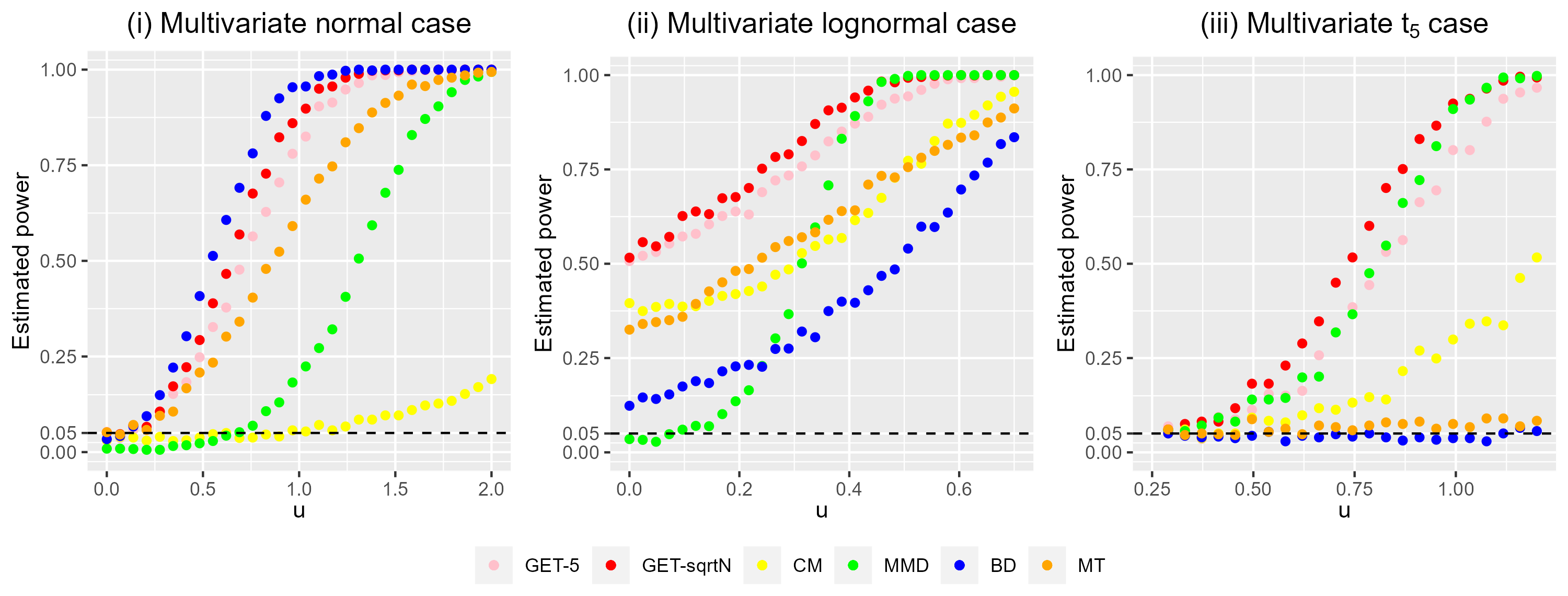
Figure 1: Estimated power of various two-sample tests.

For graph-based methods, GET or MET on the $K$-MST or the $K$-NNG are usually recommended due to their relatively high power under a broad range of alternatives [Chen and Friedman, 2017, Chu and Chen, 2019]. For simplicity, for the remaining of the paper, we refer to this subset when saying graph-based methods unless otherwise specified. In addition, this subset perform similarity across various scenarios, so we focus on GET on $K$-NNG in the main context. Some results on GET on $K$-MST are provided in Appendix A.

1.1 What might affect the performance of graph-based methods?

We first check whether outliers, defined as observations that are far from other observations, affect the performance of the graph-based methods. Figure 2 plots the estimated power of GET on $5$-NNG and $14$-NNG ($14\approx\sqrt{100+100}$) for a toy example: $X_{1},{\cdots},X_{100}\stackrel{{\scriptstyle\text{iid}}}{{\sim}}N(\mathbf{0}_{d},\mathbf{I}_{d})$, $Y_{1},{\cdots},Y_{100}\stackrel{{\scriptstyle\text{iid}}}{{\sim}}N(\mathbf{0}_{d},\sigma\mathbf{I}_{d})$, where $\sigma$ equally ranges from 1 to 1.02 with an increment of 0.001 and $d=1,000$. We purposely perturb the data in two ways:

• Random perturbation: reverse the sample labels of 5 randomly chosen nodes.

• Outlier perturbation: reverse the sample labels of 5 nodes that are furthest away from the center of the data.

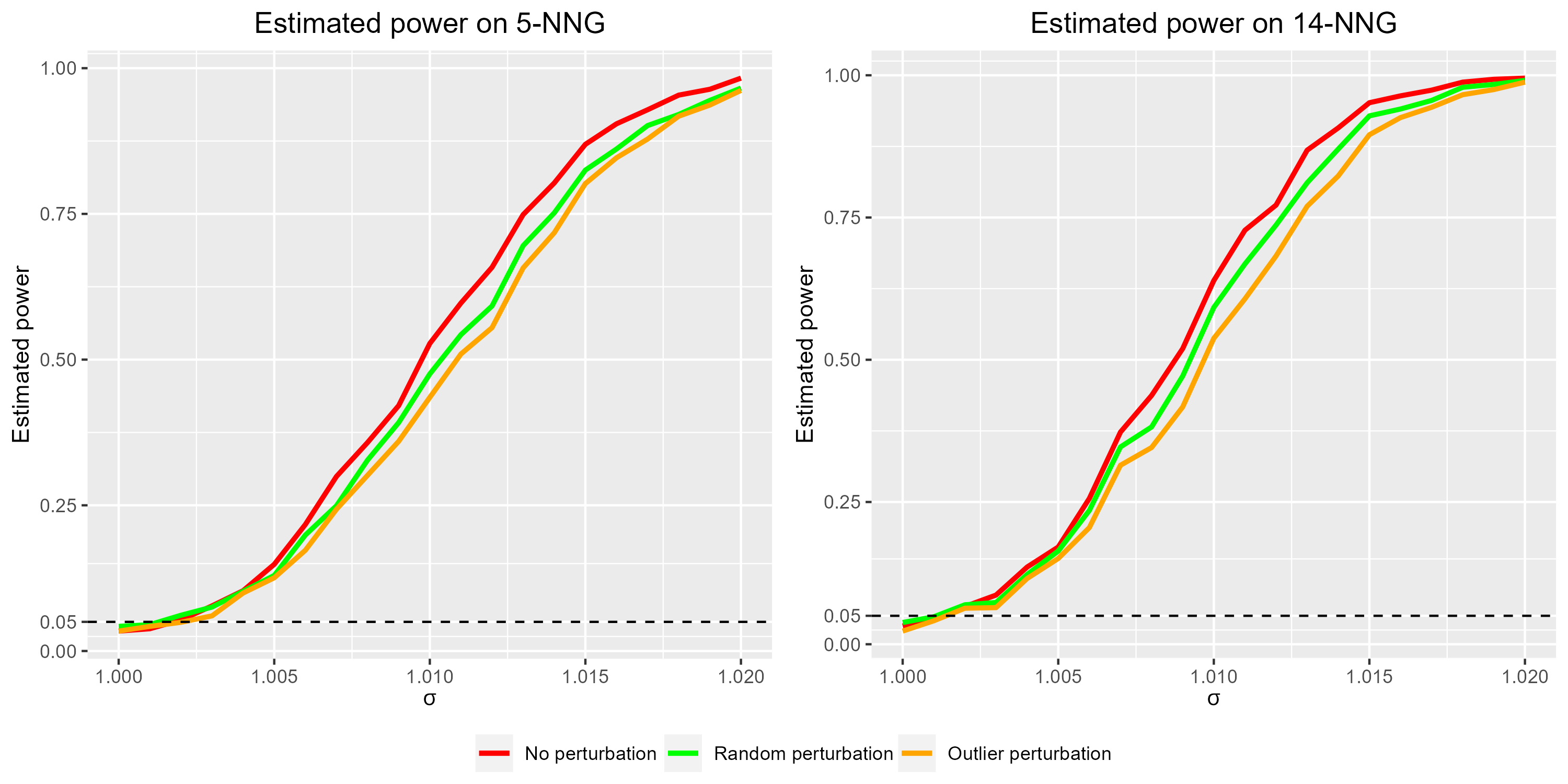
Figure 2: Estimated power of GET on the $5$-NNG and the $14$-NNG for no perturbation (red), random perturbation (green), and outlier perturbation (orange).

We see that, compared to random perturbation, mislabeling points farthest from the center decreases the power of test a bit more. However, the decrease is not too much. Hence, the method is quite robust to outliers. This is expected because the number of edges in the similarity graph that connect to the outliers is relatively small as the outliers are far away from the remaining observations and thus outliers have little effect on the method.

Then, in the same line of reasoning, if there are observations that connect to many other observations in the similarity graph, will they affect the method a lot? To check for this, we examine another type of perturbation:

• Hub perturbation: reverse the sample labels of 5 nodes with the largest degrees in the graph.

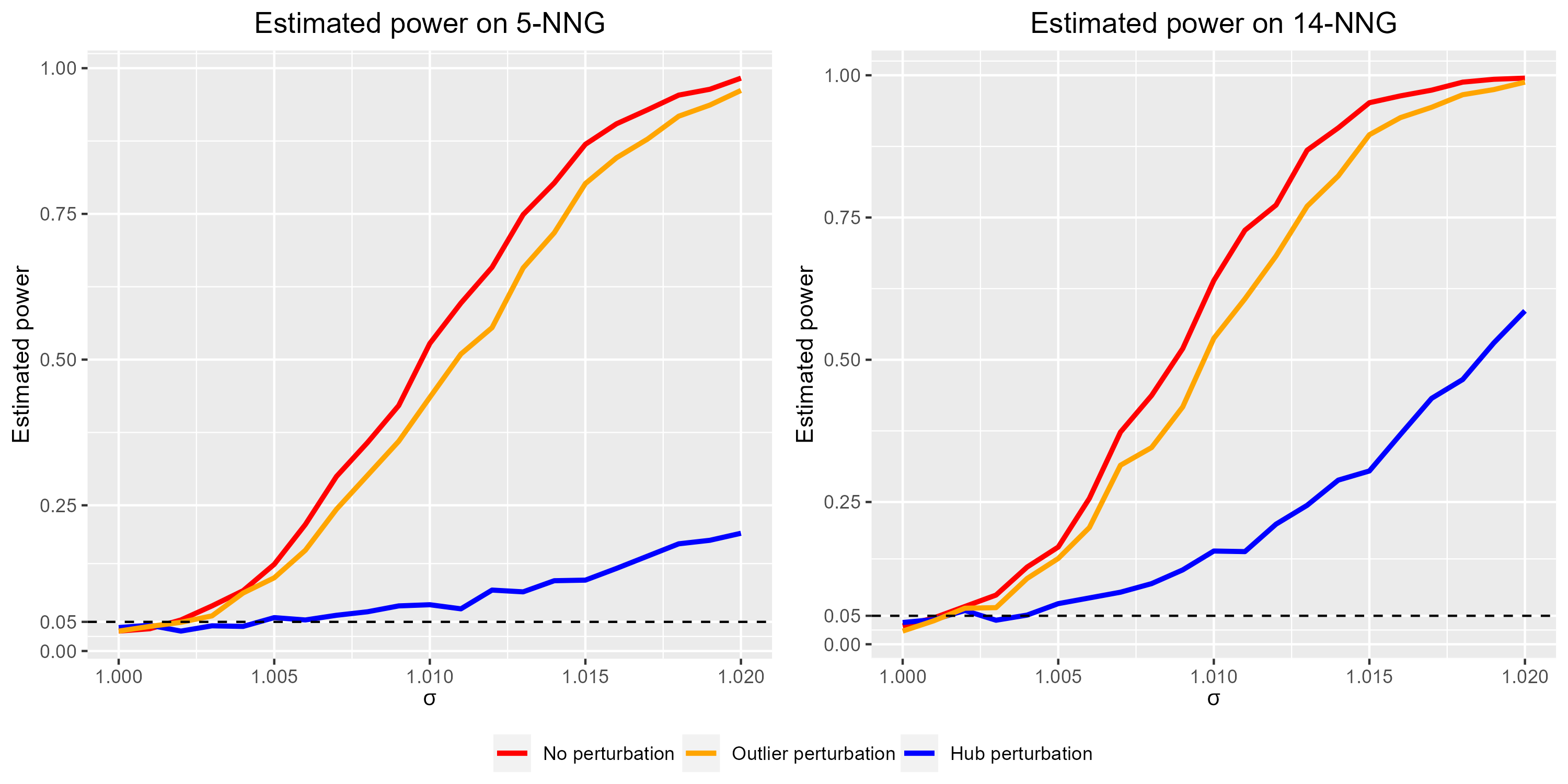
Figure 3: Estimated power of GET on the $5$-NNG and the $14$-NNG for no perturbation (red), outlier perturbation (orange), and hub perturbation (blue).

Figure 3 plots the estimated power of GET under the same setting as in Figure 2 but with hub perturbation. We see that reversing sample labels of 5 points with the largest degrees could dramatically decrease the power of the test. While using a denser graph (right panel of Figure 3) may mitigate this effect, there is still a significant decrease in power. One explanation behind the high influence of hubs on the performance of the graph-based method is that the method relies on the number of edges and a node with a large degree would affect the count more, leading to a high influence. Figure 4 plots boxplots of average degrees of perturbed points under the toy example with $\sigma=1.02$. We see that the average degree of hubs are much higher than that of other selected points.

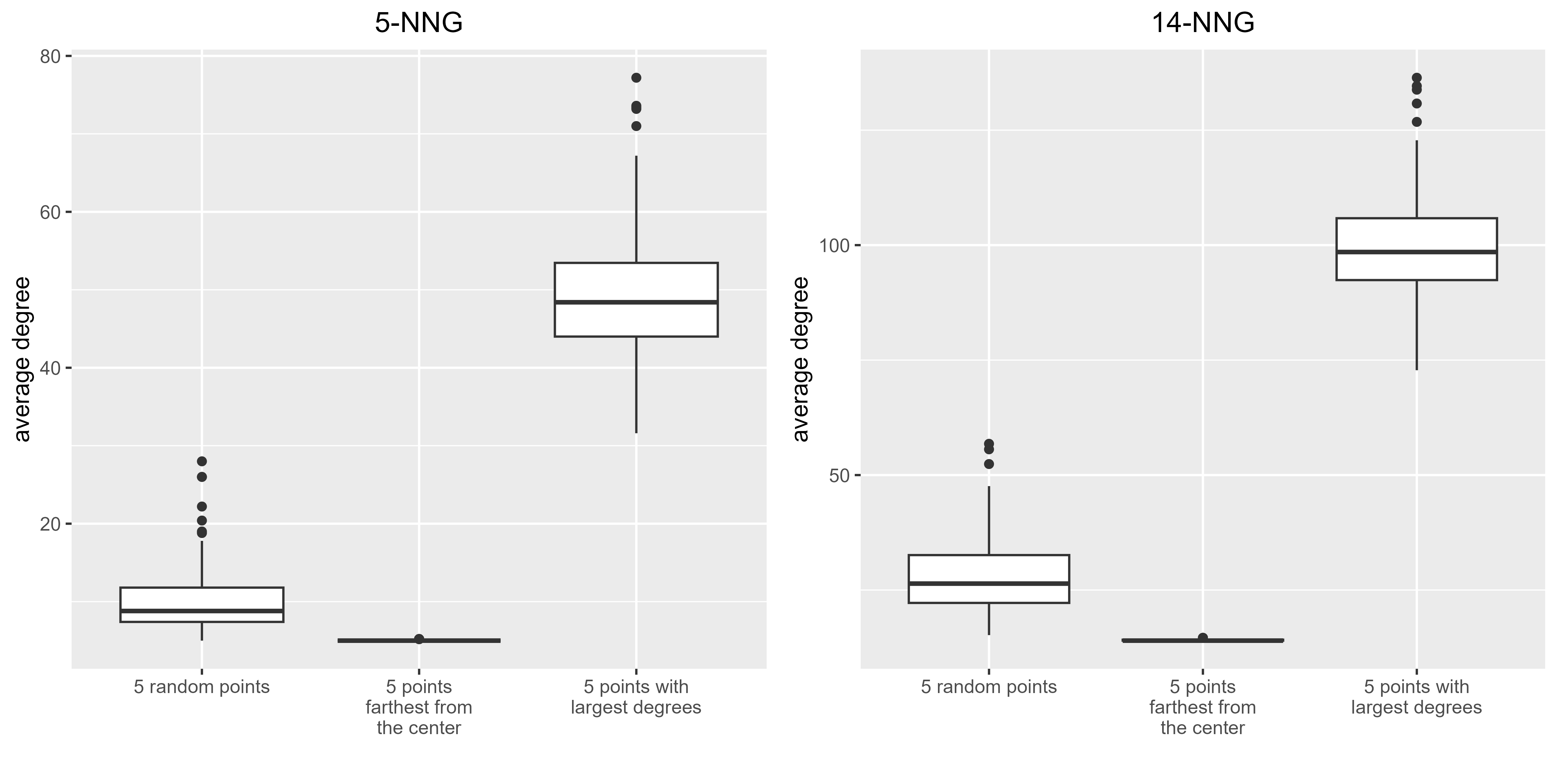
Figure 4: The average degree of perturbed points in $K$-NNG.

1.2 Relationship between hub and dimensionality

The toy example in Section 1.1 clearly demonstrates the significant influence of hubs within the $K$-NNG on the performance of graph-based methods. Here, we further examine the relationship between hubs and data dimensionality. We utilize the same toy example, maintaining a fixed Fubini norm of the covariance matrix difference at 0.3, while varying the dimensionality from 5 to 1,000. Figure 5 presents boxplots of the average degree of perturbed points in the $5$-NNG and the $14$-NNG for dimensions $5,10,50,100,200,$ and $500$.

At low dimensions ($d=5$), we observe that the average degree of hubs slightly exceeds that of 5 randomly selected nodes. As the dimensionality increases, the average degree of the randomly selected nodes remains relatively stable, while the average degree of the hubs experiences a significant escalation. This results in a pronounced overweighted influence of hubs, particularly when the dimension is not small ($d\geq 50$).

Figure 6 displays the estimated power of GET on the $5$-NNG and the $14$-NNG with perturbed data across different dimensions. The estimated power remains relatively stable across varying dimensions for both no perturbation and outlier perturbation. However, in the case of hub perturbation, the estimated power is slightly lower compared to other perturbations at low dimensions and exhibits a significant decline with a moderate increase in dimension. Notably, the estimated power with hub perturbation experiences a pronounced decrease until it reaches dimension 50, after which the decline becomes more gradual till dimension 1,000. This pattern is consistent with the observed increase in average degrees of hubs illustrated in Figure 5.

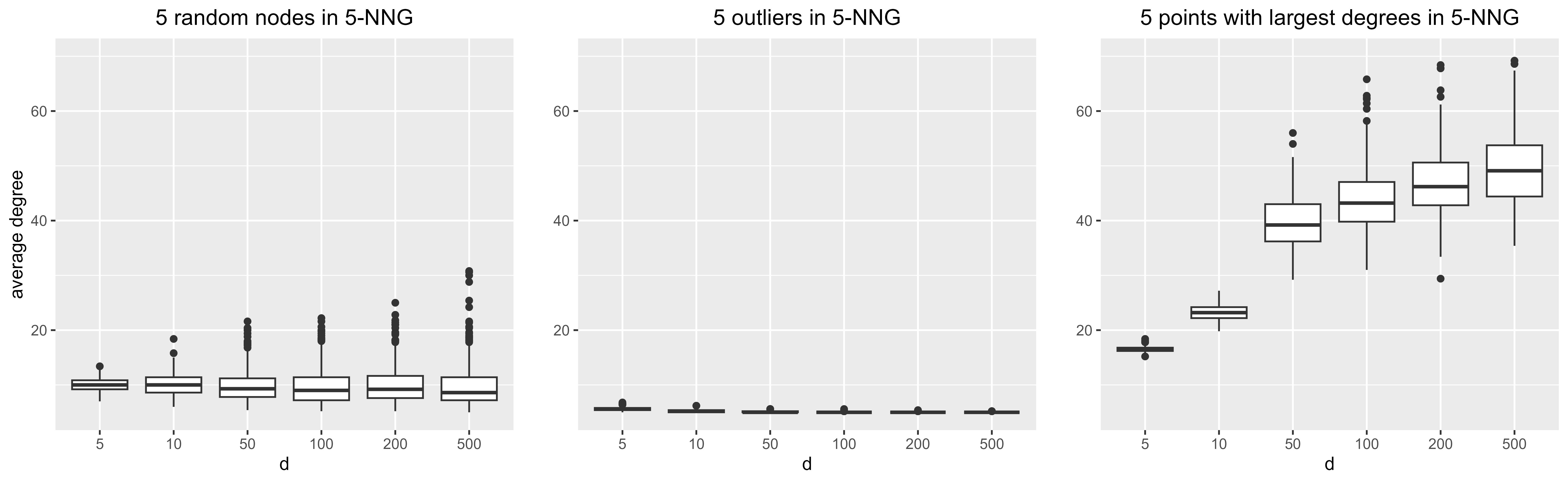
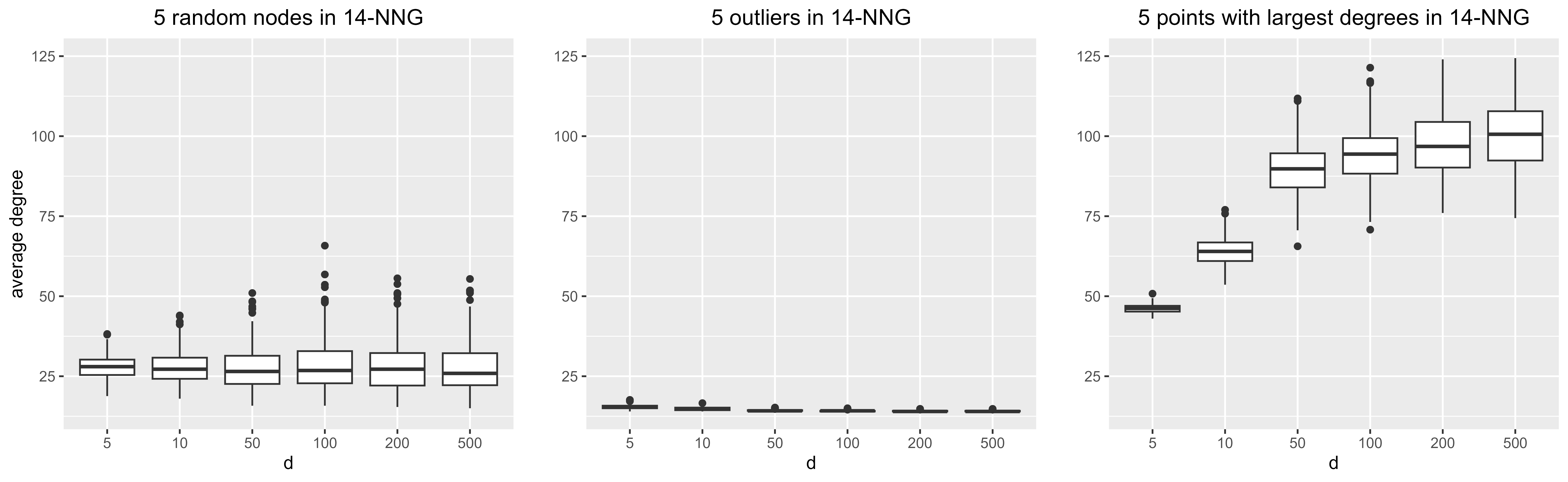
Figure 5: Boxplots of the average degree of selected points under different dimensions.

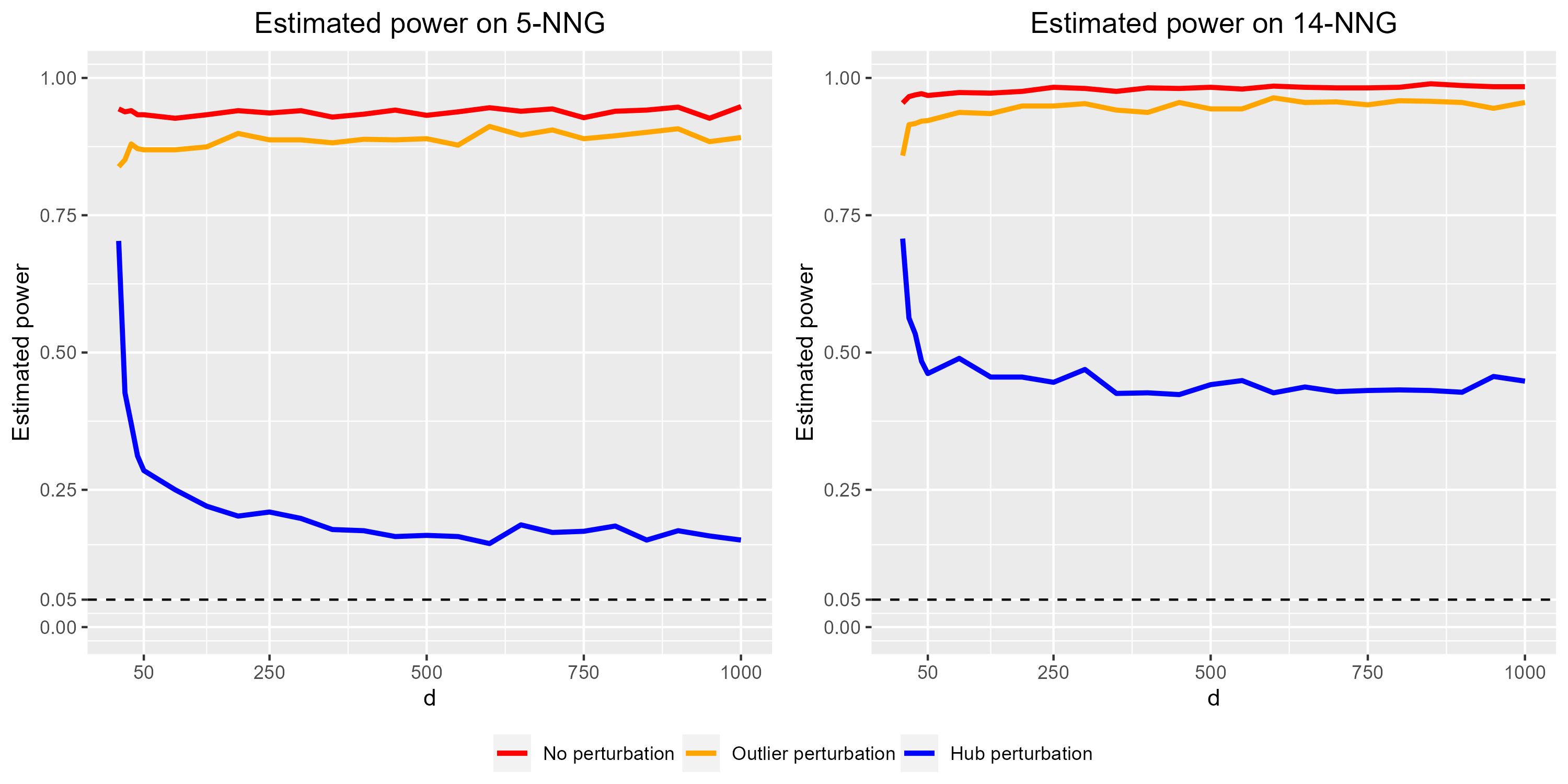
Figure 6: Estimated power of GET on the $5$-NNG and the $14$-NNG under different dimensions.

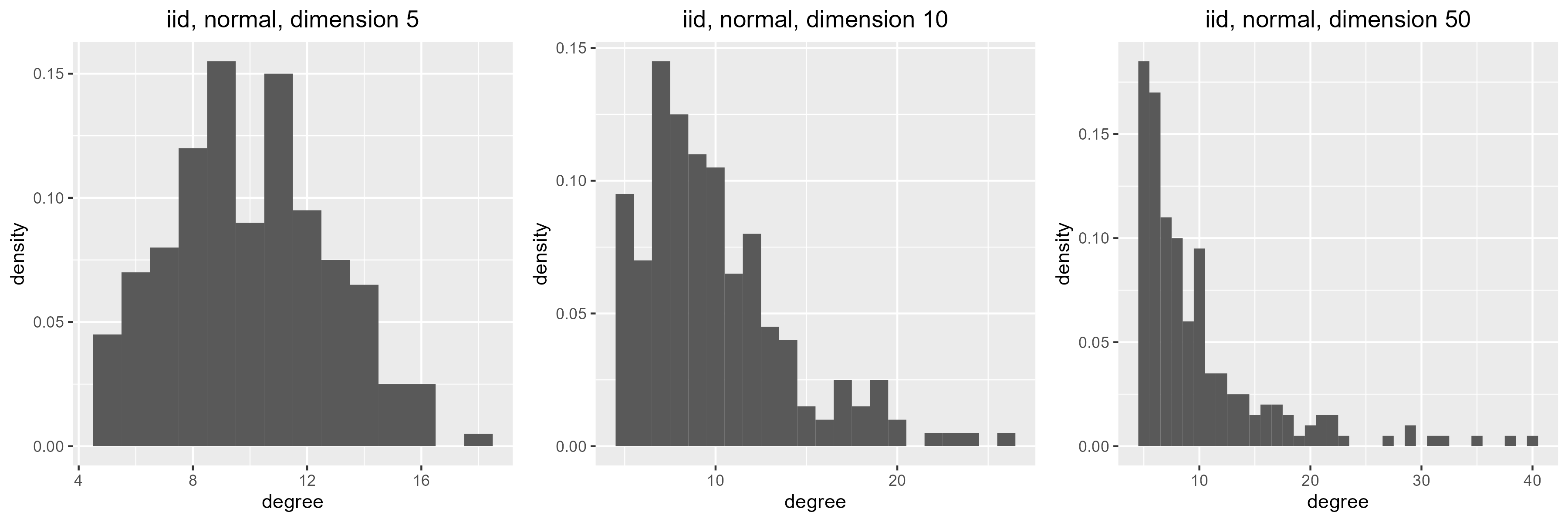
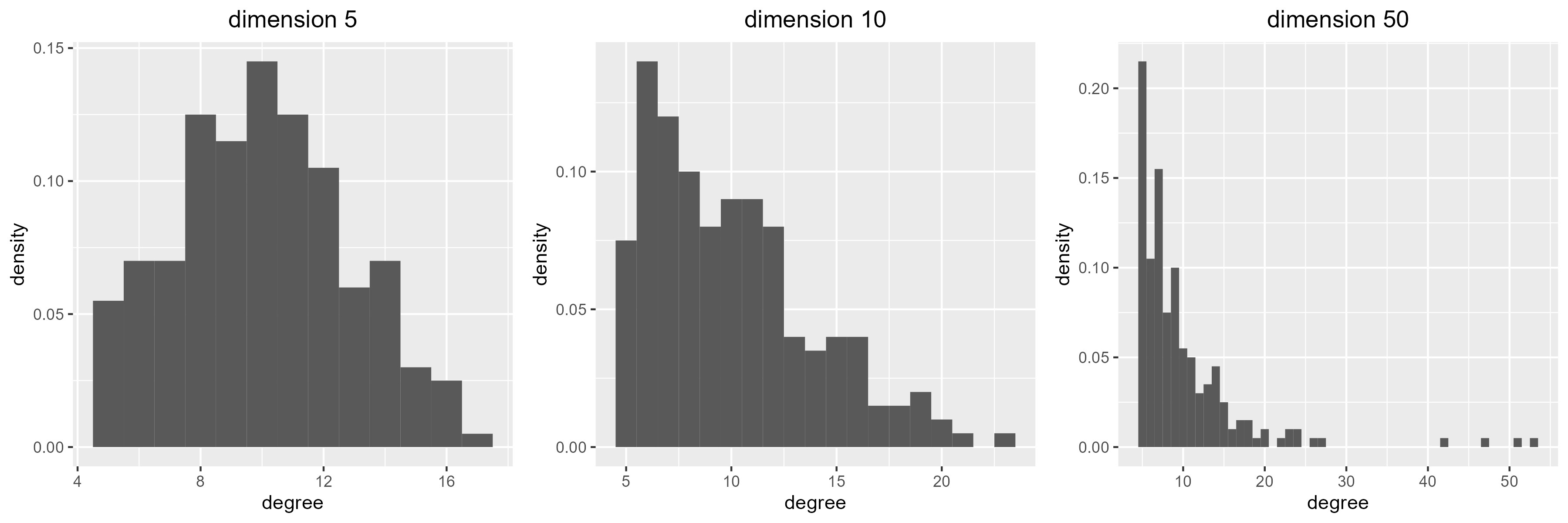
Figure 7: Degree distributions of the $5$-NNG with data under the standard multivariate normal distribution (top panel) and the toy example with a fixed Fubini norm of the covariance matrix difference at 0.3 (bottom panel).

The presence of hubs in the $K$-NNG for moderate to high dimensions can be attributed to the curse of dimensionality. Radovanovic et al. [2010] investigated the phenomenon of hubness in the $K$-NNG for data from one distribution. They demonstrated that, under commonly employed assumptions, the degree distribution becomes significantly right-skewed as dimension increases. Figure 7 plots the empirical degree distributions of the $5$-NNG with the data from the standard multivariate normal distribution (top panel) and the previous toy example with a fixed Fubini norm of the covariance matrix difference at 0.3 (bottom panel) under dimensions 5, 10 and 50. We see that, as dimension increases, both degree distributions – whether under the standard multivariate normal distribution or the toy example setting – exhibit a more pronounced right-skewed pattern.

1.3 Mitigate the effect of the curse of dimensionality for graph-based methods

In terms of the test statistic, Chen and Friedman [2017] had renovated the OET statistic to the GET statistic to take into account the pattern caused by the curse of dimensionality, and thus making the test statistic more robust to the curse of dimensionality. However we see from previous examples that the recommended graphs, $K$-NNG (in Section 1.1 and 1.2) and $K$-MST (in Appendix A), are also affected by the curse of dimensionality. In this paper, we focus on constructing similarity graphs that are robust to the curse of dimensionality. In particular, since hubs emerge naturally as dimension increases and graph-based methods are susceptible to hubs, we propose to construct robust graphs by penalizing the presence of hubs. The detailed procedure for constructing these robust graphs is provided in Section 2. By using the robust similarity graphs, we can significantly mitigate the impact of the curse of dimensionality.

Figure 8 displays the estimated power of GET on the $K$-robust nearest neighbor graph ($K$-RNNG) (solid lines) under the same setting as in Figures 2 and 3 (dotted lines). We see that, even though the hub perturbation (blue lines) still cause some power decrease, the decrease is much less significant compared to that using the $K$-NNG (dashed blue lines).

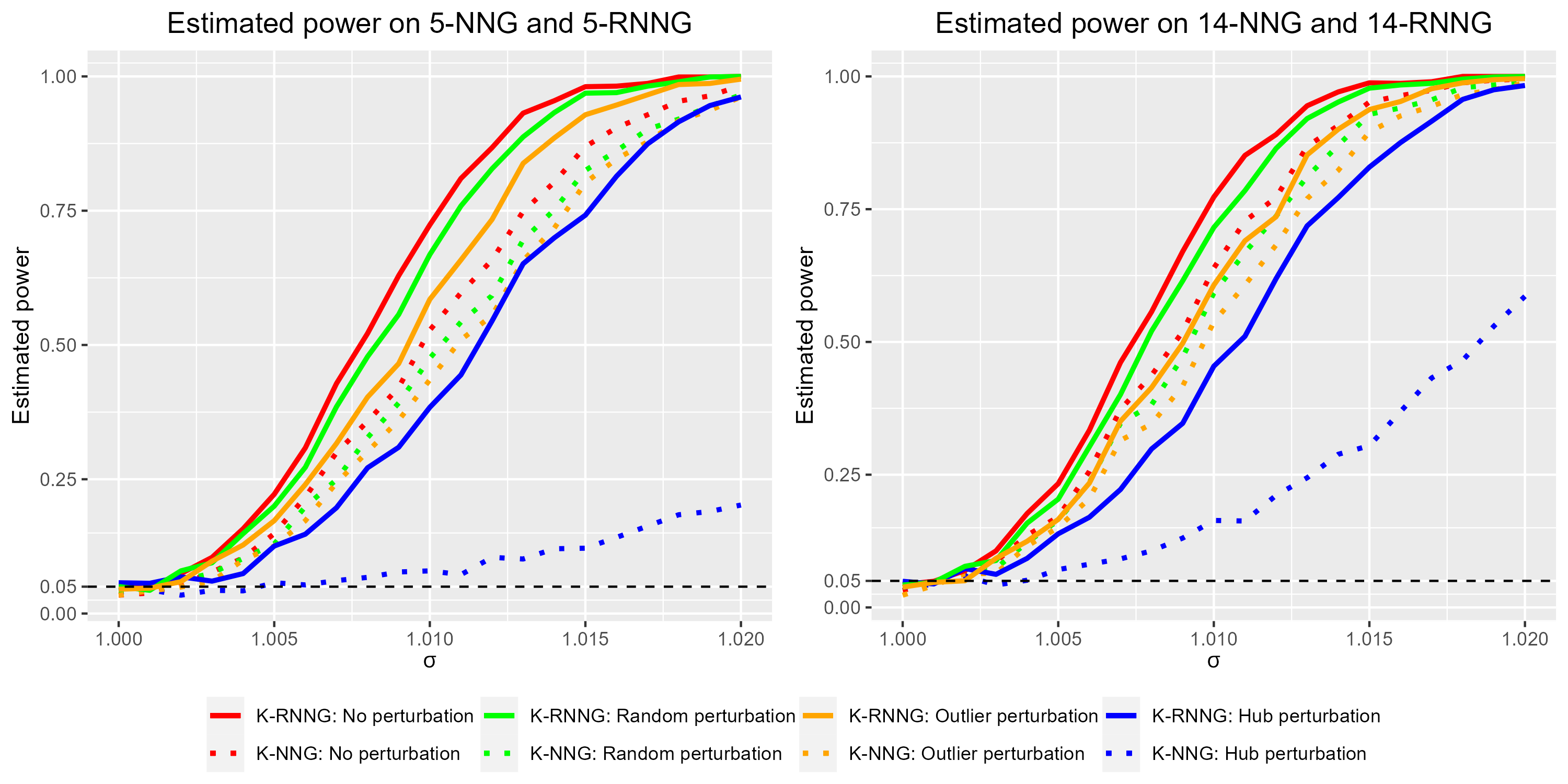
Figure 8: Estimated power of GET on the $K$-NNG and the $K$-RNNG.

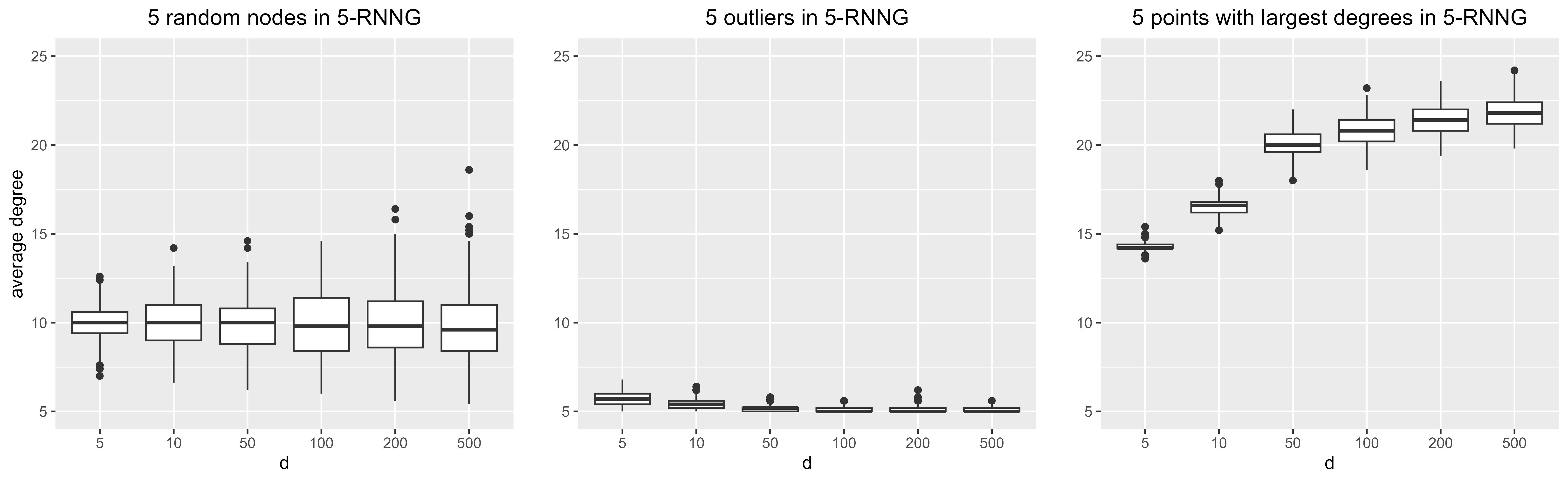
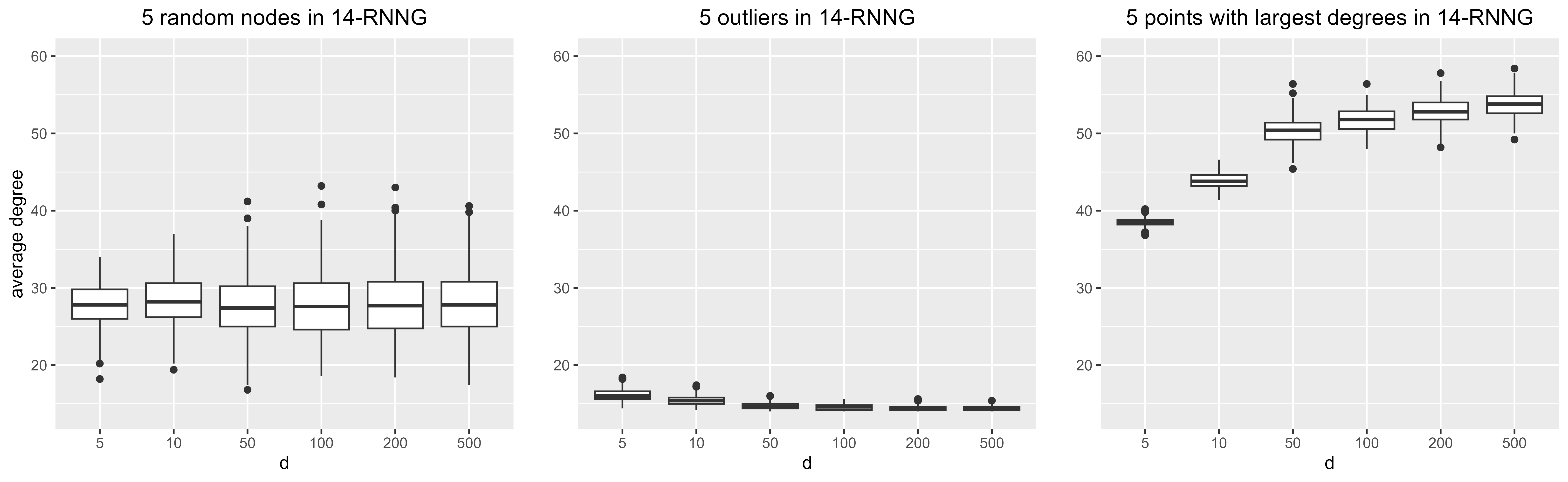
Figure 9: Boxplots of the average degree of selected points in the $5$-RNNG and the $14$-RNNG across different dimensions.

Figure 9 displays the boxplots of the average degree of perturbed points in the $5$-RNNG and $14$-RNNG under a similar setting as in Figure 5 for dimensions 5, 10, 50, 100, 200, and 500. We see that the average degrees of the five largest degrees in the 5-RNNG and the 14-RNNG are considerably smaller compared to their counterparts in the 5-NNG and the 14-NNG, as presented in Figure 5. For instance, when the dimension increases from 5 to 1,000, the average degree of the five largest degrees in the $5$-NNG rises from 17 to 50. However, in the $5$-RNNG, this average degree only experiences a modest increase, from 14 to approximately 22.

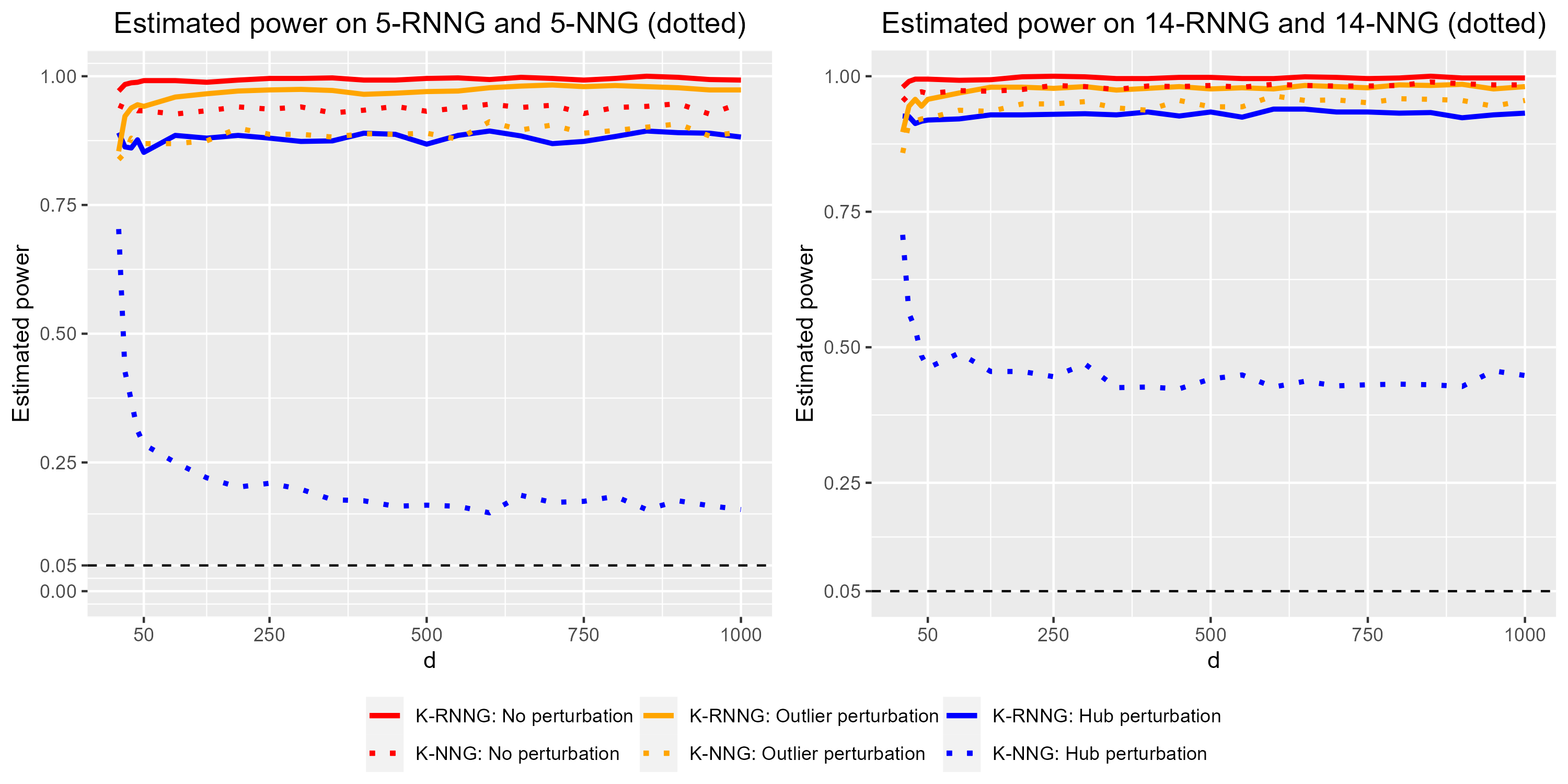
Figure 10: Estimated power of GET on 5-RNNG and 14-RNNG with different dimensions.

Figure 10 displays the estimated power of GET on the $K$-RNNG across different dimensions. It is evident that the estimated power of GET on $K$-RNNG with hub perturbation no longer decreases as dimension increases.

1.3.1 Power improvement without perturbation

Besides enhancing the robustness of graph-based methods against hub perturbations, the robust graphs also improves the overall power of these methods. This improvement is evident in Figures 8 and 10, where the solid red lines surpass the dotted red lines that represent scenarios without perturbations. To check that this effect is not coincidental, we further examine the power of GET on both the 5-RNNG and on the 5-NNG across various settings:

• $X_{1},{\cdots},X_{m}\stackrel{{\scriptstyle\text{iid}}}{{\sim}}N(\mathbf{0}_{d},\Sigma_{d}(0.5))$,  $Y_{1},{\cdots},Y_{n}\stackrel{{\scriptstyle\text{iid}}}{{\sim}}N(\frac{\delta}{\sqrt{d}}\mathbf{1}_{d},$ $\Sigma_{d}(0.5))$,

• $X_{1},{\cdots},X_{m}\stackrel{{\scriptstyle\text{iid}}}{{\sim}}N(\mathbf{0}_{d},\Sigma_{d}(0.5))$, $Y_{1},{\cdots},Y_{n}\stackrel{{\scriptstyle\text{iid}}}{{\sim}}N(\frac{\delta}{\sqrt{d}}\mathbf{1}_{d},$ $\Sigma_{d}(0.5)+\frac{\delta}{\sqrt{d}}\mathbf{I}_{d})$,

• $X_{1},{\cdots},X_{m}\stackrel{{\scriptstyle\text{iid}}}{{\sim}}\text{Lognormal}(\mathbf{0}_{d},\Sigma_{d}(0.5))$, $Y_{1},{\cdots},Y_{n}\stackrel{{\scriptstyle\text{iid}}}{{\sim}}\text{Lognormal}(\frac{\delta}{\sqrt{d}}\mathbf{1}_{d},\Sigma_{d}(0.5))$,

• $X_{1},{\cdots},X_{m}\stackrel{{\scriptstyle\text{iid}}}{{\sim}}\text{Multivariate t}_{5}(\mathbf{0}_{d},\Sigma_{d}(0.5))$, $Y_{1},{\cdots},Y_{n}\stackrel{{\scriptstyle\text{iid}}}{{\sim}}\text{Multivariate t}_{5}(\frac{\delta}{\sqrt{d}}\mathbf{1}_{d},\\ \Sigma_{d}(0.5)+\frac{\delta}{\sqrt{d}}\mathbf{I}_{d})$,

where $m=n=100$, $d=500$. Setting 1 involves mean shift under the multivariate normal distribution. Settings 2, 3, and 4 introduce both mean shift and scale difference under different distributions.

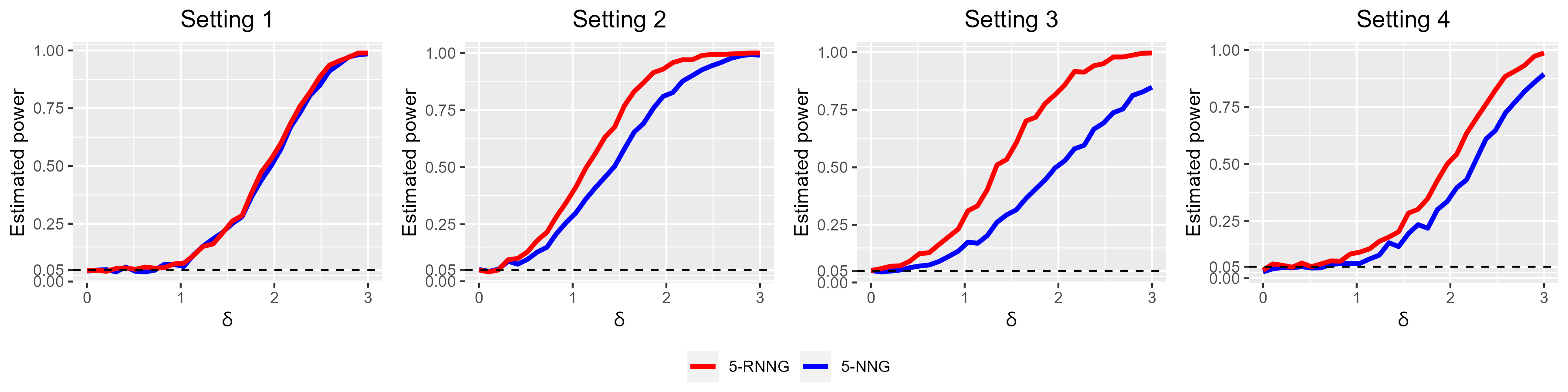
Figure 11: Estimated power of GET on $5$-RNNG (red) and GET on $5$-NNG (blue).

Figure 11 illustrates the estimated power of GET on both the $5$-RNNG and the $5$-NNG. In Setting 1 where only mean difference exists, GET on the $5$-RNNG and GET on $5$-NNG exhibit similar performance. However, in Settings 2, 3, and 4, which involve both mean shift and scale difference, GET on the $5$-RNNG exhibits substantially higher power compared to GET on the $5$-NNG. This finding suggests that the $5$-RNNG is particularly advantageous in scenarios where scale difference exists across distributions.

1.4 Organization

The rest of the paper is organized as follows. In Section 2, we introduce the robust similarity graph in details, investigate the asymptotic properties of the GET statistic on the proposed robust graph, and explore the choice of hyper-parameter $\lambda$. Section 3 presents a comparative analysis of the performance of GET on the $K$-NNG, $K$-MST, and $K$-RNNG, along with other popular methods, in both two-sample testing and change-point detection problems through numeric studies.

2 Robust similarity graphs

Given $N$ observations, $Z_{1},{\cdots},Z_{N}$, and a distance metric $D(\cdot,\cdot)$, we define $R_{i}(Z_{j})$ to be the rank of the distance $D(Z_{i},Z_{j})$ within the set of distances $\{D(Z_{i},Z_{l}):l\neq i\}$. Then, the $K$-NNG minimizes $\sum_{i=1}^{N}\sum_{x\in C_{i}}R_{i}(x)$ over all possible sets $C_{i}$, where $C_{i}$ contains $K$ observations excluding $Z_{i}$. In a graph $G$, let $|G_{i}|$ be the degree of the $i$-th node, taking into account both the in-degree and out-degree. We define the $K$-robust nearest neighbor graph ($K$-RNNG) as the graph that minimizes the objective function (1) over all sets $C_{i}$ that contain $K$ observations excluding $Z_{i}$:

$$\sum_{i=1}^{N}\sum_{x\in C_{i}}R_{i}(x)+\lambda\sum_{i=1}^{N}|G_{i}|^{2}.$$ (1)

Here, $\lambda$ is a hyper-parameter and its choice is discussed in Section 2.2. Optimizing the objective function (1) is a combinatorial problem and finding the global optimum is typically difficult. In this paper, we provide a greedy algorithm (Algorithm 1) as a practical approach. While this algorithm may not guarantee the global optimum, we find it to be effective enough in practice.

Algorithm 1 Constructing the $K$-robust nearest neighbor graph

1:Initialize $G$ with the $K$-NNG, and compute the value of the objective function (1) on $G$ and store it as $L$.

2:Randomly permute the order of nodes and indicate them to be $1,{\cdots},N$. For $i$ from $1$ to $N$,

• Compute $W_{i}(j)=R_{i}(Z_{j})+\lambda(|G_{j}^{\star}|+1)^{2}$, where $|G_{j}^{\star}|=|G_{j}|-1$ if node $j$ is one of neighbors of node $i$; otherwise $|G_{j}^{\star}|=|G_{j}|$;

• Find $K$ nodes with the $K$ smallest $W_{i}(j)$’s among $\{W_{i}(j)\}_{j=1,{\cdots},i-1,i+1,{\cdots},N}$;

• Compute objective function (1) with node $i$ connecting to these $K$ nodes found in Step 2.2 and denote it as $L^{\star}$;

• If $L^{\star}<L$, update the graph by pointing node $i$ to the $K$ nodes found Step 2.2 and Let $L=L^{\star}$; otherwise do not change the graph or the value of $L$.

3:Repeat Step 2 until no node can find neighbors with a lower $L^{\star}$.

Remark 1

In the objective function (1), the regularization term employs the total degree $|G_{i}|$, which is equally to use the in-degree as the out-degree for each node is fixed to be $K$.

Remark 2

The objective function (1) is not limited to ranks. We could use a distance metric $D(\cdot,\cdot)$ directly, and the $K$-RNNG can be obtained by solving

$$\min_{C_{i}\text{'s}}\sum_{i=1}^{N}\sum_{x\in C_{i}}D(Z_{i},x)+\lambda\sum_{i=1}^{N}|G_{i}|^{2}$$

$$\text{s.t. }Z_{i}\notin C_{i},|C_{i}|=K.$$

The choice of using ranks in the objective function here that necessitates only the information of closeness brings a distance-free graph. It allows to study the theoretical property of the robust graph without considering the specific distance metric.

Remark 3

A similar idea can be used to extend the $K$-MST to the robust $K$-MST. Let $R(Z_{i},Z_{j})$ be the rank of distance $D(Z_{i},Z_{j})$ in the set of all pairwise distances. The robust $K$-MST is a $K$-spanning tree $T$, which minimize the objective function

$$\sum_{(z_{i},z_{j})\in T}R(z_{i},z_{j})+\lambda\sum_{i=1}^{N}|G_{i}|^{2}.$$

2.1 Asymptotic properties of the GET statistic on the $K$-RNNG

Zhu and Chen [2021] derived so far the best sufficient conditions on undirected graphs for the validity of the asymptotic distribution of the GET statistic. In this section, we extend their results to directed graphs and demonstrate that the $K$-RNNG graphs meet these conditions with an appropriate choice of $\lambda$. Before stating these results, we first define some essential notations.

Given a directed graph $G$ built on the pooled observations $Z_{1},{\cdots},Z_{N}$ $(Z_{i}=X_{i},$ $i=1,{\cdots},m;$ $Z_{j+m}=Y_{j},$ $j=1,{\cdots},n;N=m+n)$. The pair $(i,j)$ (the order matters) represents a directed edge pointing from node $i$ to node $j$. We define $|G|$ to be the number of directed edges in the graph $G$. For each node $i$, we define $G_{i}$ as the set of edges with one node $i$, $G_{i,2}$ as the set of edges sharing at least one node with an edge in $G_{i}$, $node_{G_{i}}$ as the set of nodes that are connected in $G_{i}$ excluding the node $i$, and $node_{G_{i,2}}$ as the set of nodes that are connected in $G_{i,2}$ excluding the node $i$. We further define $N_{0}$ to be the number of edges whose reversed edge is also in $G$, i.e. $N_{0}=\sum_{\left(i,j\right)\in G}1_{\{(j,i)\in G\}}$, $\tilde{d_{i}}$ to be the centered degree, i.e. $\tilde{d_{i}}=|G_{i}|-\frac{2|G|}{N}$, and $N_{sq}$ to be the number of combinations of 4 edges that form a square. Let $V_{G}=\sum_{i=1}^{N}\tilde{d_{i}}^{2}=\sum_{i=1}^{N}|G_{i}|^{2}-\frac{4|G|^{2}}{N}$ representing the variation of degrees.

Besides, we use $\xrightarrow{\mathcal{D}}$ to denote convergence in distribution, and use ‘the usual limit regime’ to refer $N\rightarrow\infty$ and $\lim_{N\rightarrow\infty}\frac{m}{N}=p\in(0,1)$. In the following, $a_{n}=o(b_{n})$ or $a_{n}\prec b_{n}$ means that $a_{n}$ is dominated by $b_{n}$ asymptotically, i.e. $\lim_{n\rightarrow\infty}\frac{a_{n}}{b_{n}}=0$, $a_{n}\precsim b_{n}$ or $a_{n}=O(b_{n})$ means $a_{n}$ is bounded above by $b_{n}$ (up to a constant factor) asymptotically, and $a_{n}=\Theta(b_{n})$ or $a_{n}\asymp b_{n}$ means that $a_{n}$ is bounded both above and below by $b_{n}$ (up to constant factors) asymptotically. We use $a\wedge b$ for $\min\{a,b\}$. For two sets $S_{1}$ and $S_{2}$, $S_{1}\backslash S_{2}$ is used for the set that contains elements in $S_{1}$ but not in $S_{2}$.

Let $l_{i}$ be the sample group label of $i$-th node defined as

$$l_{i}=\left\{\begin{aligned} 1&\text{ if node $i$ is from sample X}\\ 2&\text{ if node $i$ is from sample Y.}\end{aligned}\right.$$

Let $R_{1}$ and $R_{2}$ be the number of within-sample edges in sample $X$ and sample $Y$, respectively,

$$R_{1}=\sum_{(i,j)\in G}1_{\{l_{i}=l_{j}=1\}},\quad R_{2}=\sum_{(i,j)\in G}1_{\{l_{i}=l_{j}=2\}}.$$

Then, the GET statistic $S$ can be expressed as

$$S=\begin{pmatrix}R_{1}-\textsf{E}_{\text{P}}(R_{1}),&R_{2}-\textsf{E}_{\text{P}}(R_{2})\end{pmatrix}\times\left(\textsf{Var}_{\text{P}}\binom{R_{1}}{R_{2}}\right)^{-1}\begin{pmatrix}R_{1}-\textsf{E}_{\text{P}}(R_{1})\\ R_{2}-\textsf{E}_{\text{P}}(R_{2})\end{pmatrix},$$

where $\textsf{E}_{\text{P}}$, $\textsf{Var}_{\text{P}}$ and $\textsf{Cov}_{\text{P}}$ are the expectation, variance and covariance under the permutation null distribution which places probability $1/{N\choose m}$ on each selection of $m$ observations among all $N$ observations as sample X.

Zhu and Chen [2021] established the sufficient conditions for the asymptotic distribution of the test statistic via the ‘locSCB’ approach. This approach relies on the equivalence between the permutation null distribution and the conditional Bootstrap null distribution. The Bootstrap null distribution assigns each observation to either sample $X$ or sample $Y$ independently, with probabilities $\frac{m}{N}$ and $\frac{n}{N}$, respectively. Conditioning on the number of observations assigned to sample $X$ being $m$, the Bootstrap null distribution becomes the permutation null distribution. The authors applied the Stein’s method that considers the first neighbor dependency under the Bootstrap null distribution to derive asymptotic multivariate normality. We here adopt a similar idea to derive the sufficient conditions for the directed graph. A challenge with directed graphs is their allowance for multiple edges between two nodes, so it requires meticulous consideration of certain graph-related quantities. The conditions are provided in Theorem 1, and the proof of the theorem is in Supplemental Material.

Theorem 1

For a directed graph $G$ with $|G|=O(N^{\alpha}),1\leq\alpha<2$, under conditions

$$\sum_{i=1}^{N}\left|G_{i}\right|^{2}=o\left(|G|^{\frac{3}{2}}\right),\sum_{i=1}^{N}\left|\tilde{d_{i}}\right|^{3}=o(V_{G}^{\frac{3}{2}}),\sum_{i=1}^{N}\tilde{d_{i}}^{3}=o(V_{G}\sqrt{|G|}),$$

$$\sum_{i=1}^{N}\sum_{(i,j)\text{ or }(j,i)\in G_{i}}^{(i,k)\text{ or }(k,i)\in G_{i},j\neq k}\tilde{d_{j}}\tilde{d_{k}}=o(|G|V_{G}),\quad N_{sq}=o(|G|^{2}).$$

in the usual limit regime, we have $S\xrightarrow{\mathcal{D}}\chi_{2}^{2}$ under the permutation null distribution.

These sufficient conditions stated in Theorem 1 are applicable to any general directed graphs. For the $K$-RNNG, a more concise result can be obtained. By selecting an appropriate value for $\lambda$, all the sufficient conditions in Theorem 1 are satisfied for the $K$-RNNG. The main result is stated in Theorem 2 with the proof provided in Supplemental Material.

Theorem 2

Let $Q_{N}$ be the random variable generated from the degree distribution of the $K$-RNNG with $N$ nodes. Assume $K=\Theta(1)$ and if $\lambda$ is chosen such that $\textsf{Var}(Q_{N})>0$ and $\max\{Q_{N}\}\precsim N^{\frac{1}{2}-\beta}$ for some $\beta>0$, we have $S\xrightarrow{\mathcal{D}}\chi_{2}^{2}$ under the permutation null distribution in the usual limit regime.

Remark 4

Theorem 2 requires that the variance of degree distribution of the $K$-RNNG is asymptotically bounded away from zero when choosing $\lambda$. This is to ensure that the GET statistic is well defined – when $\textsf{Var}(Q_{N})=0$, the degrees of all nodes are the same and $\textsf{Var}_{\text{P}}\binom{R_{1}}{R_{2}}$ becomes singular. This situation arises when an extremely large $\lambda$ is used. Additionally large values of $\lambda$ diminish the utilization of the similarity information contained in the first term of the objective function (1), making such choices of $\lambda$ less desirable. Therefore, we tend not to choose a very large $\lambda$ in practice.

Theorem 3 (Consistency under fixed dimensions)

For two samples generated from two continuous multivariate distributions in Euclidean space with a fixed dimension, if the graph is the $K$-RNNG with $K=\Theta(1)$ and $\lambda\geq 0$, GET is consistent against all alternatives in the usual limiting regime.

Theorem 4 (Consistency under high dimensions)

Assume distributions $F_{X}$ and $F_{Y}$ satisfy Assumptions 1 and 2 in [Biswas et al., 2014], and $\lim_{d\rightarrow\infty}\textsf{E}(||X-\textsf{E}(X)||_{2}^{2})/d=\sigma_{1}^{2}$, $\lim_{d\rightarrow\infty}\textsf{E}(||Y-\textsf{E}(Y)||_{2}^{2})/d=\sigma_{2}^{2}$ and $\lim_{d\rightarrow\infty}(||\textsf{E}(X)-\textsf{E}(Y)||_{2}^{2})/d=v^{2}$, where $X\sim F_{X}$, $Y\sim F_{Y}$ and $d$ is the dimension. Without loss of generality, we assume that $\sigma_{1}^{2}>\sigma_{2}^{2}$. Then, for GET on the $K$-RNNG with $0<\lambda<(\sqrt{8NK+4N-8K}-\sqrt{8NK})^{2}/16$ and $\min\{m,n\}>K+2\lambda+\sqrt{8\lambda KN}$, we have $\lim_{d\rightarrow\infty}P(S>\chi_{2}^{2}(1-\alpha))=1$, for any fixed $\alpha\in(0,1)$, when either of the following conditions hold:

• $|\sigma_{1}^{2}-\sigma_{2}^{2}|<v^{2}$, $N>2.5+\frac{\xi}{K}+\sqrt{0.25+3\frac{\xi}{K}+\frac{\xi^{2}}{K^{2}}}$,

• $N>\frac{n^{2}\xi^{2}}{2m^{2}K^{2}}\left(\sqrt{\frac{K}{\lambda}}+\sqrt{\frac{K}{\lambda}+\frac{2mK}{n\xi}(1+\frac{K}{2\lambda}+\frac{mK}{n\xi}-K)}\right)^{2}$, $\sigma_{1}^{2}-\sigma_{2}^{2}>v^{2}$,

• $N>\frac{m^{2}\xi^{2}}{2n^{2}K^{2}}\left(\sqrt{\frac{K}{\lambda}}+\sqrt{\frac{K}{\lambda}+\frac{2nK}{m\xi}(1+\frac{K}{2\lambda}+\frac{nK}{m\xi}-K)}\right)^{2}$, $\sigma_{2}^{2}-\sigma_{1}^{2}>v^{2}$,

where $\xi=\chi_{2}^{2}(1-\alpha)$.

Theorem 3 studies the consistency of GET on $K$-RNNG under the fixed dimension as the sample size goes to infinity. Theorem 4 studies the consistency as the dimension goes to infinity. The proofs of these theorems are in Supplemental Material. For Theorem 4, although we usually don’t know which case $\sigma_{1}^{2}$, $\sigma_{2}^{2}$ and $v^{2}$ satisfy, we can always choose the largest $N$ among three cases. For instance, with $\alpha=0.05$, $\lambda=0.3$, $m=n$ and $K=5$, it requires $N\geq 69$. With $\alpha=0.05$, $\lambda=0.3$, $m/n=2$ or $n/m=2$ and $K=5$, it requires $N\geq 214$.

2.2 Choice of $\lambda$

To assess the impact of $\lambda$ on the power of GET on the 5-RNNG, we vary the value of $\lambda$ and look into the empirical power of the test. We consider the following scenarios including symmetric distribution, asymmetric distribution, and heavy-tailed distribution.

• $X_{1},{\cdots},X_{m}\stackrel{{\scriptstyle\text{iid}}}{{\sim}}N(\mathbf{0}_{d},\Sigma_{d}(0.5))$, $Y_{1},{\cdots},Y_{n}\stackrel{{\scriptstyle\text{iid}}}{{\sim}}N(\mathbf{0}_{d},\delta\Sigma_{d}(0.5))$ with $m=200$, $n=100$, $d=500$ and $\delta=1.03$;

• $X_{1},{\cdots},X_{m}\stackrel{{\scriptstyle\text{iid}}}{{\sim}}\text{lognormal}(\mathbf{0}_{d},\Sigma_{d}(0.5))$, $Y_{1},{\cdots},Y_{n}\stackrel{{\scriptstyle\text{iid}}}{{\sim}}\text{lognormal}(\delta\mathbf{1}_{d},\Sigma_{d}(0.5))$ with $m=100$, $n=200$, $d=1000$ and $\delta=0.05$;

• $X_{1},{\cdots},X_{m}\stackrel{{\scriptstyle\text{iid}}}{{\sim}}\text{lognormal}(\mathbf{0}_{d},\Sigma_{d}(0.5))$, $Y_{1},{\cdots},Y_{n}\stackrel{{\scriptstyle\text{iid}}}{{\sim}}\text{lognormal}(\mathbf{0}_{d},\delta\Sigma_{d}(0.5))$ with $m=100$, $n=100$, $d=100$ and $\delta=1.15$;

• $X_{1},{\cdots},X_{m}\stackrel{{\scriptstyle\text{iid}}}{{\sim}}\text{t}_{5}(\mathbf{0}_{d},\Sigma_{d}(0.5))$, $Y_{1},{\cdots},Y_{n}\stackrel{{\scriptstyle\text{iid}}}{{\sim}}\text{t}_{5}(\mathbf{0}_{d},\delta\Sigma_{d}(0.5))$ with $m=100$, $n=100$, $d=500$ and $\delta=1.35$;

• $X_{1},{\cdots},X_{m}\stackrel{{\scriptstyle\text{iid}}}{{\sim}}\text{t}_{5}(\mathbf{0}_{d},\Sigma_{d}(0.5))$, $Y_{1},{\cdots},Y_{n}\stackrel{{\scriptstyle\text{iid}}}{{\sim}}\text{t}_{5}(\delta\mathbf{1}_{d},\Sigma_{d}(0.5))$ with $m=300$, $n=100$, $d=500$ and $\delta=0.095$.

where $\delta$ is chosen so that the tests have moderate power when $\lambda$ is equal to zero.

Figure 12 presents the estimated power of the test across different values of $\lambda$. The results indicate a rapid increase in power as $\lambda$ rises from 0 to 0.3, followed by a slower rate of improvement. To determine a default value for $\lambda$, we employ the elbow method, which suggests a value of 0.3 would be appropriate.

In Figure 13, we plot the relationship between the maximum center degree and $\lambda$. It is evident that the maximum degree experiences a rapid decline when $\lambda$ increases from 0 to 0.3, followed by a slower rate of decrease. This observation aligns with the trend depicted in Figure 12, which showcases the estimated power. Consequently, a practical data-driven approach to select an appropriate $\lambda$ is to plot the maximum degrees for various values of $\lambda$ and identify the point at which the maximum degree exhibits minimal changes.

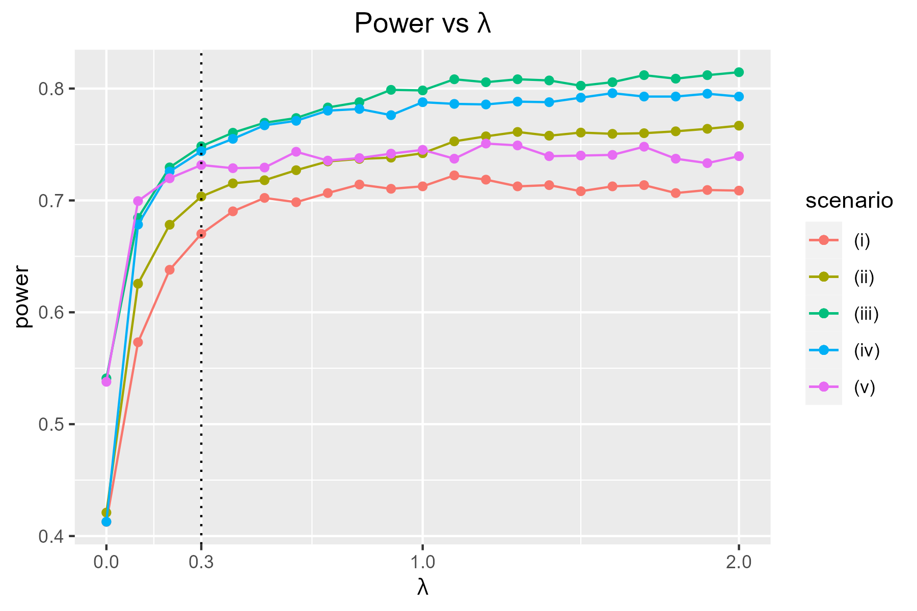
Figure 12: The estimated powers w.r.t $\lambda$ under various distribution settings.

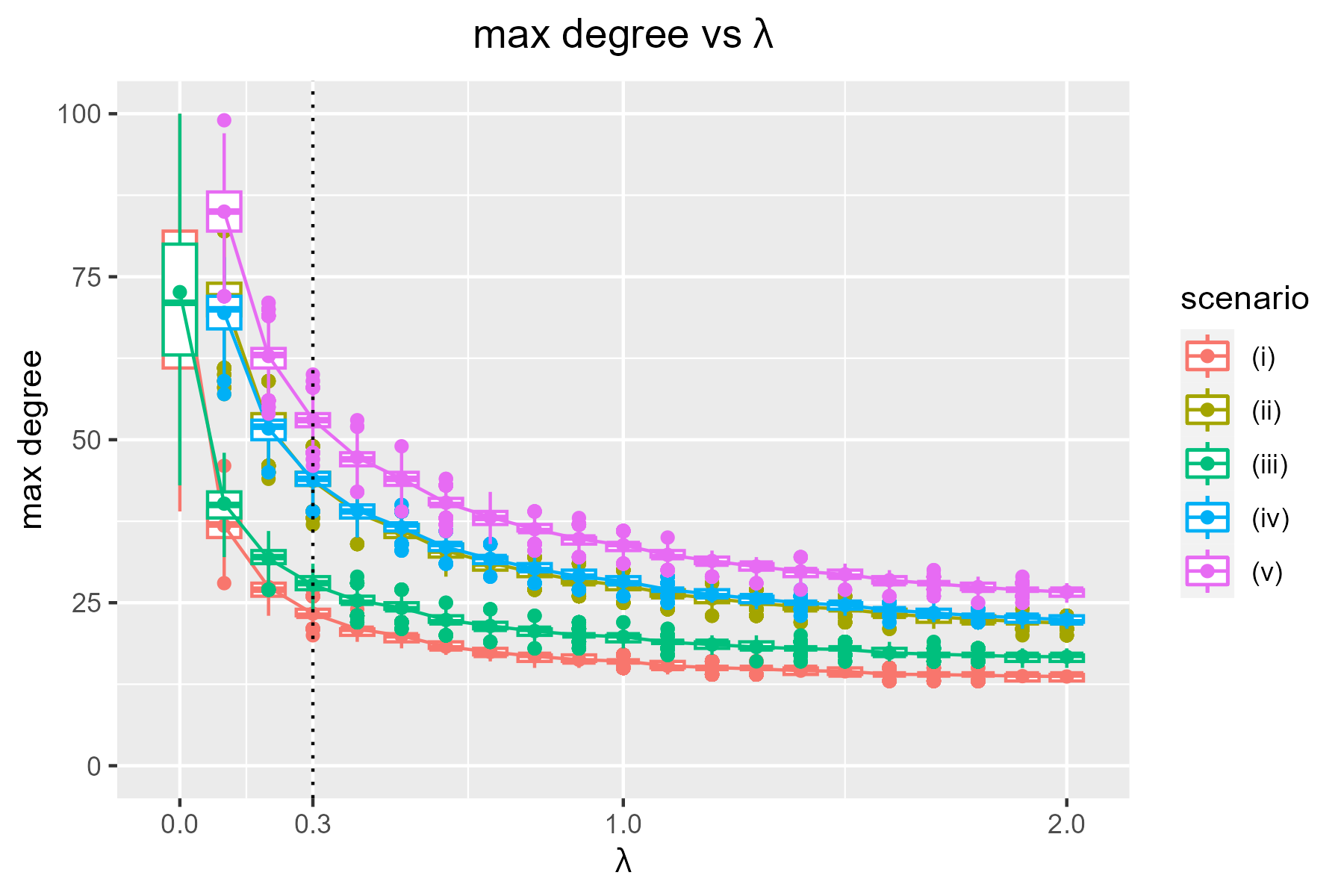
Figure 13: Max degree w.r.t $\lambda$ under various distribution settings.

3 Numerical studies

In this section, we evaluate the performance of GET on $K$-RNNG by comparing it with other state-of-the-art methods in both the two-sample testing and change-point detection problems.

3.1 Two-sample testing

We consider GET on 5-RNNG (New), 5-MST, $\sqrt{N}$-MST, and other popular tests: the cross-match test [Rosenbaum, 2005] (CM), the Ball divergence test [Pan et al., 2018] (BD), the mutivariate rank-based test [Deb and Sen, 2021] (MT), the Adaptable Regularized Hotelling’s $\text{T}^{2}$ test [Li et al., 2020] (ARHT) and the kernel test based on minimum mean discrepancy [Gretton et al., 2012a] (MMD), under the following simulation scenarios:

• $X_{1},{\cdots},X_{m}\stackrel{{\scriptstyle\text{iid}}}{{\sim}}N(\mathbf{0}_{d},\Sigma_{d}(0.5))$, $Y_{1},{\cdots},Y_{n}\stackrel{{\scriptstyle\text{iid}}}{{\sim}}N(\frac{\delta}{\sqrt{d}}\mathbf{1}_{d},$ $\Sigma_{d}(0.5)+\frac{\delta}{\sqrt{d}}\mathbf{I}_{d})$,

• $X_{1},{\cdots},X_{m}\stackrel{{\scriptstyle\text{iid}}}{{\sim}}{Lognormal}(\mathbf{0}_{d},\Sigma_{d}(0.6))$, $Y_{1},{\cdots},Y_{n}\stackrel{{\scriptstyle\text{iid}}}{{\sim}}{Lognormal}(\mathbf{\Delta},\Sigma_{d}(0.2))$,

• $X_{1},{\cdots},X_{m}\stackrel{{\scriptstyle\text{iid}}}{{\sim}}\text{Multivariate t}_{2}(\mathbf{0}_{d},\Sigma_{d}(0.5))$, $Y_{1},{\cdots},Y_{n}\stackrel{{\scriptstyle\text{iid}}}{{\sim}}\text{Multivariate t}_{2}(\frac{\delta}{\sqrt{d}}\mathbf{1}_{d},\\ \Sigma_{d}(0.5)+\delta\mathbf{I}_{d})$,

• $X_{1},{\cdots},X_{m}\stackrel{{\scriptstyle\text{iid}}}{{\sim}}\text{Multivariate t}_{1}(\mathbf{0}_{d},\Sigma_{d}(0.5))$, $Y_{1},{\cdots},Y_{n}\stackrel{{\scriptstyle\text{iid}}}{{\sim}}\text{Multivariate t}_{1}(\frac{\delta}{\sqrt{d}}\mathbf{1}_{d},\\ \Sigma_{d}(0.5)+\frac{\delta}{2}\mathbf{I}_{d})$,

where $\mathbf{\Delta}$ a $d$-dimensional vector with first $\sqrt{d}$ elements equal to $\delta$ and the remaining elements equal to $0$.

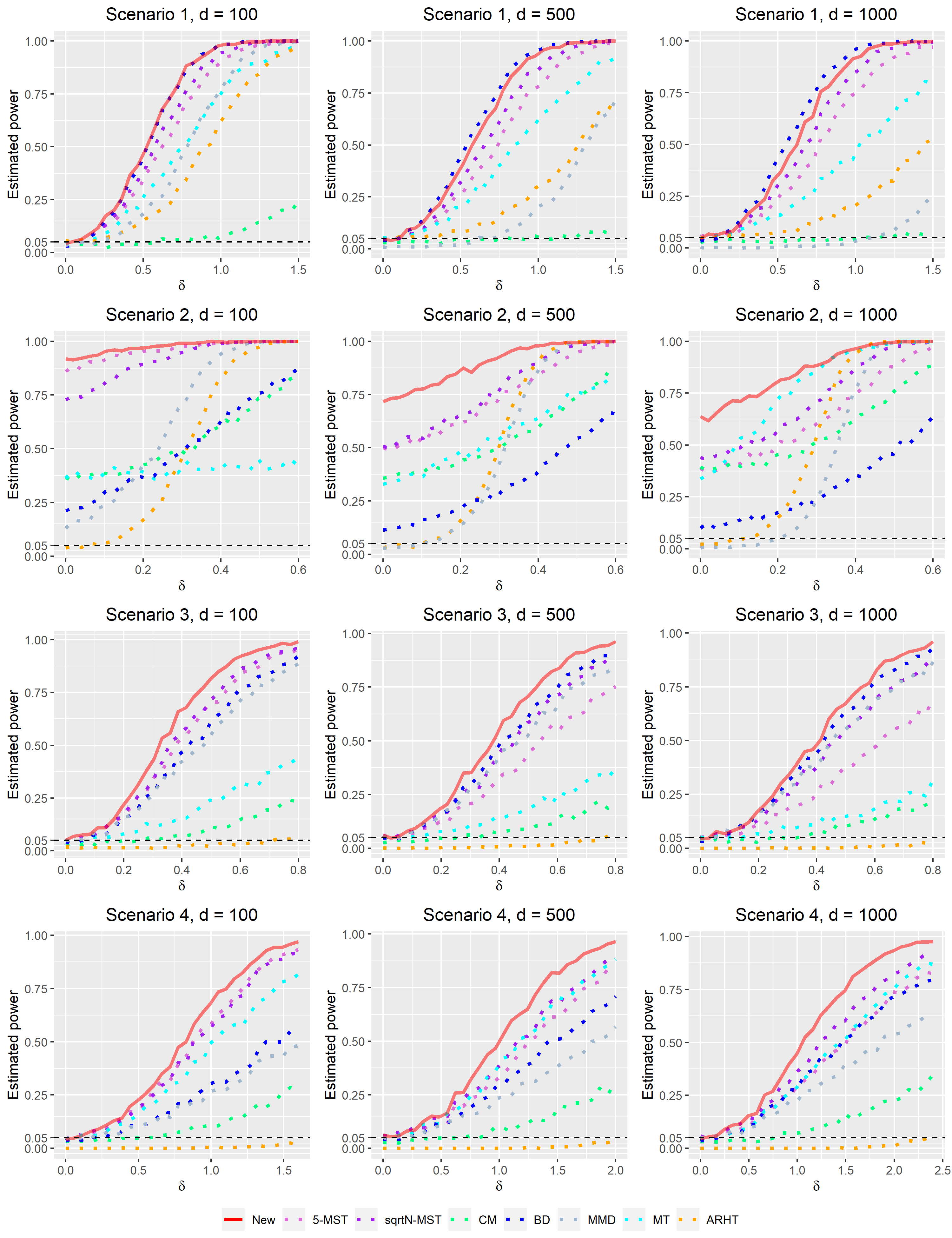
Figure 14: Estimated powers of two-sample tests under different settings.

In each scenario, we set $m=n=100$ and $d=50,500,1000$. The estimated powers computed from 1000 repetitions are plotted in Figure 14. Firstly, we observe that the empirical sizes of the GET on the $5$-RNNG are well controlled across different scenarios (at $\delta=0$ in Secenario 1, 3 and 4). In Scenario 1 and 2, although the power of the new test is marginally inferior to the BD’s power, which demonstrates the maximum power in these scenarios, it excels in Scenario 3 and 4 and has a significant improvement over BD in scenario 4. Moreover, the new test consistently surpasses the GET on $5$-MST and the GET on $\sqrt{N}$-MST across all scenarios. This result underpins the advantages of employing $K$-RNNG, considering the tests only differ in their graph structures.

3.2 Change-point detection

For graph-based change-point detection, MET is often recommended over GET [Chu and Chen, 2019, Liu and Chen, 2022, Song and Chen, 2022], so we check the performance of both MET on $5$-RNNG and GET on $5$-RNNG in this section. We include in the comparison GET scan statistic on $5$-MST, MET scan statistic on $5$-NNG, and the distance-based approach in [Matteson and James, 2014, James and Matteson, 2013] (e.divisive), and consider the following simulation settings:

• $X_{1},{\cdots},X_{\tau}\stackrel{{\scriptstyle\text{iid}}}{{\sim}}N(\mathbf{0}_{d},\Sigma_{d}(0.5))$, $X_{\tau+1},{\cdots},X_{N}\stackrel{{\scriptstyle\text{iid}}}{{\sim}}N(\frac{\delta}{\sqrt{d}}\mathbf{1}_{d},$ $\Sigma_{d}(0.5)+\frac{\delta}{\sqrt{d}}{\mathbf{I}_{d}})$,

• $X_{1},\cdots,X_{\tau}\stackrel{{\scriptstyle\text{iid}}}{{\sim}}N(\mathbf{0}_{d},\mathbf{I}_{d})$, $X_{\tau+1},{\cdots},X_{N}\stackrel{{\scriptstyle\text{iid}}}{{\sim}}N(\mathbf{0}_{d},\Sigma_{d}(\delta))$,

• $X_{1},\cdots,X_{\tau}\stackrel{{\scriptstyle\text{iid}}}{{\sim}}\text{Multivariate t}_{5}(\mathbf{0}_{d},\Sigma_{d}(0.5))$, $X_{\tau+1},{\cdots},$ $X_{N}\stackrel{{\scriptstyle\text{iid}}}{{\sim}}\text{Multivariate t}_{5}(\frac{\delta}{d}\mathbf{1}_{d},\\ \delta\mathbf{I}_{d}+\Sigma_{d}(0.5))$.

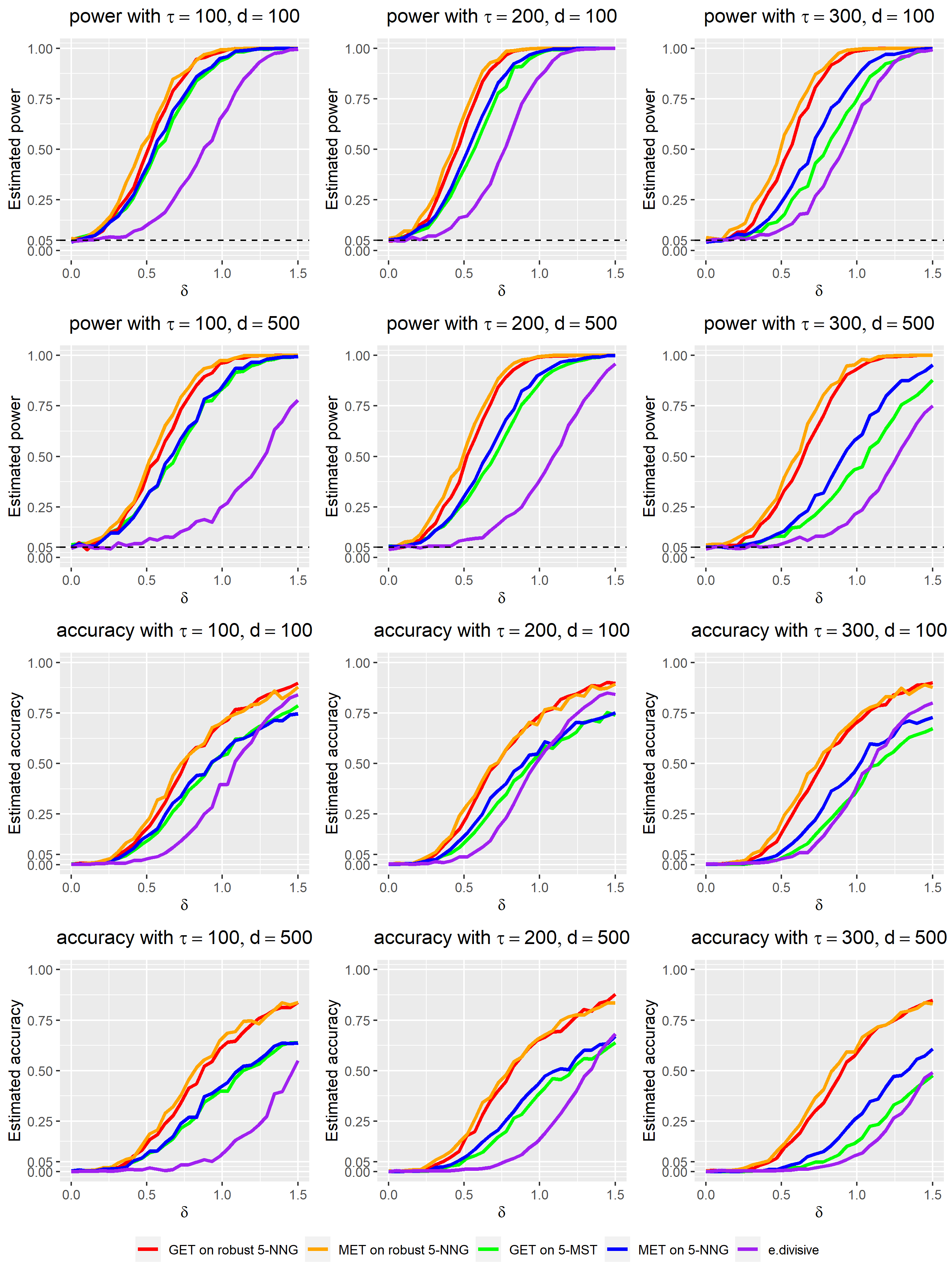
Figure 15: Estimated power and accuracy of change-point detection methods for Setting 1.

In each setting, we set $N$ to be 400, the true change-point $\tau$ to be at $100,200$ or $300$, and $d$ to be $100$ or $500$. The estimated power is computed as the proportion of trials with significant $p$-value among 1000 trials, and the accuracy is computed as the proportion of trials with significant $p$-value and estimated change-point $\hat{\tau}$ satisfying $|\hat{\tau}-\tau|\leq 10$, among 1000 trials. The estimated power and accuracy under Setting 1 are plotted in Figure 15, and the estimated power and accuracy under other settings are plotted in Figures 20 and 21 in Appendix B. We see that the MET and GET scan statistics on the $5$-RNNG have good power and accuracy in all settings, while others may perform well under some settings but poorly for some others.

4 Conclusion and discussion

In this paper, we propose a novel similarity graph to overcome the curse of dimensionality by imposing penalties on high-degree hubs, effectively reducing their impact. Our empirical investigations demonstrate that incorporating this new graph can significantly enhance the effectiveness of graph-based methods in the domains of both two-sample testing and offline change-point detection problems. However, the advantages of this robust similarity graph extend beyond these specific applications. It holds the potential to elevate performance and alleviate the detrimental effects of the curse of dimensionality across various fields, including online change-point detection, independence testing, classifications, and clustering. For instance, by adopting the new $K$-RNNG, the efficiency of methods like GET or MET in online change-point detection can be further amplified. Similarly, the performance of classification algorithms currently relying on the conventional $K$-NNG can experience substantial improvements through the incorporation of the new $K$-RNNG.

Appendix A Effect of hubs on GET on $K$-MST

We apply GET on $K$-MST under the same setting in Section 1.1. Figure 16 shows the estimated power of GET on $K$-MST with and without perturbations, from which we can see that the performance of GET on $K$-MST is similar to that of GET on $K$-NNG and hubs have dominated effect on the power of GET on $K$-MST compared with other nodes.

We also investigate the effect of hubs and dimensionality in the $K$-MST. Figure 17 depicts the average degree of perturbed points in $5$-MST and $14$-MST with $\sigma=1.02$ and $d=1000$. Figure 18 shows the average degrees of perturbed points $5$-MST and $14$-MST with ranging dimensions. Figure 19 shows the estimated power of GET on $5$-MST and $14$-MST with ranging dimensions.

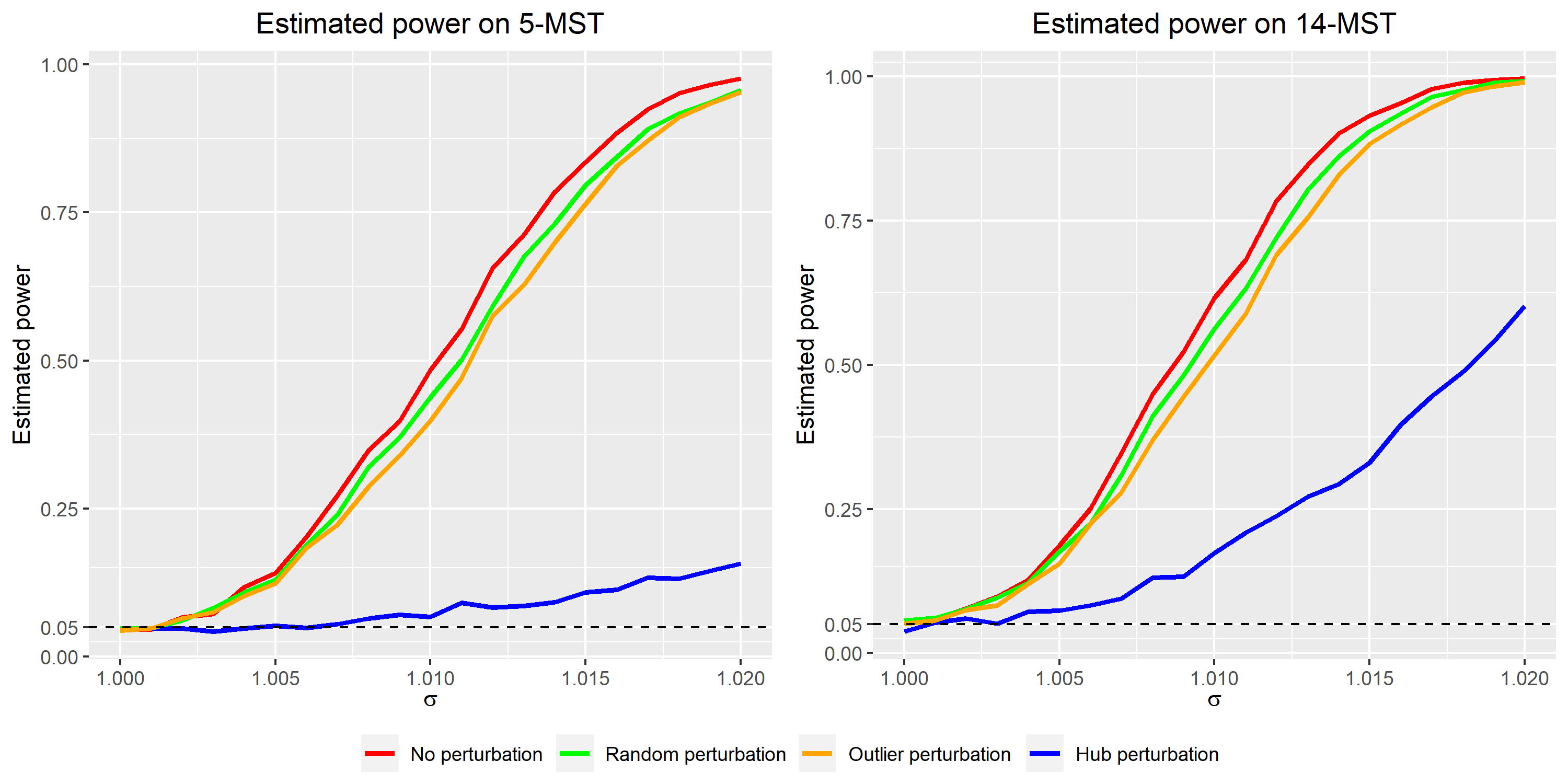
Figure 16: Estimated power of GET on the $5$-MST and the $14$-MST.

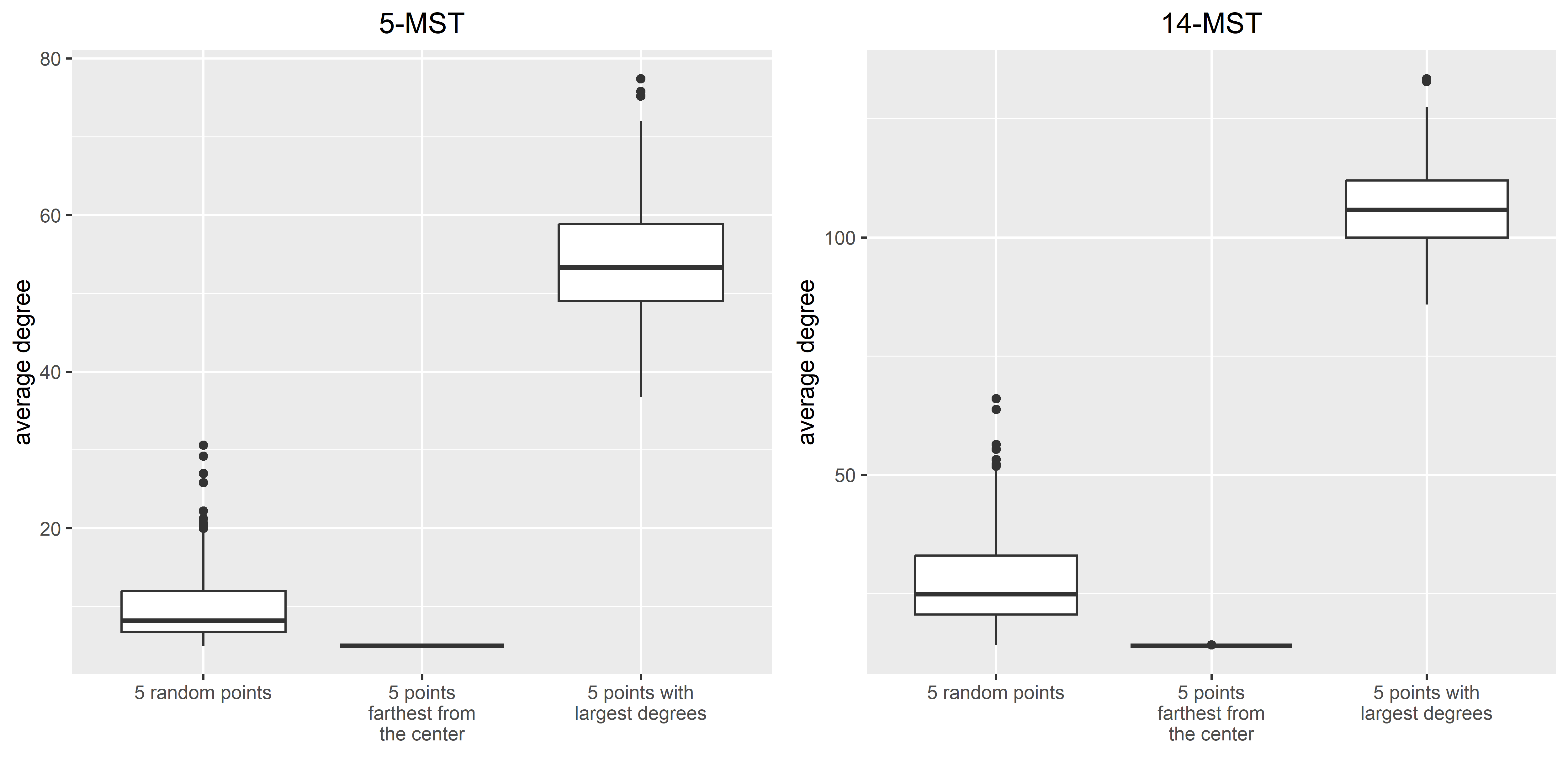
Figure 17: The average degrees of perturbed points in $K$-MST.

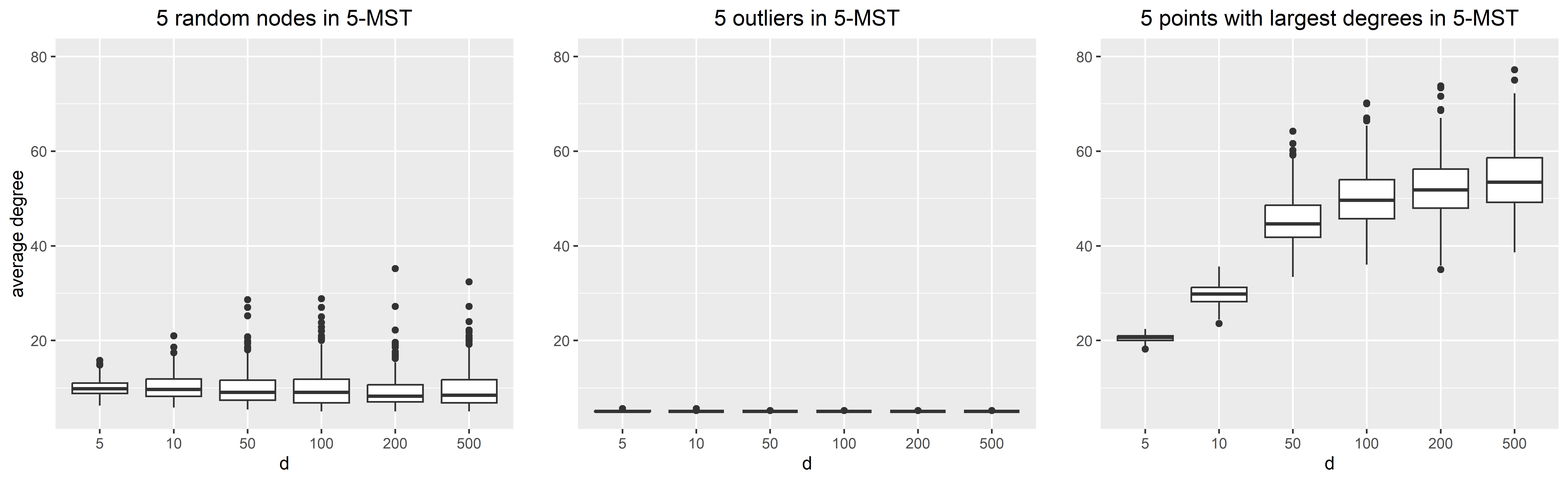
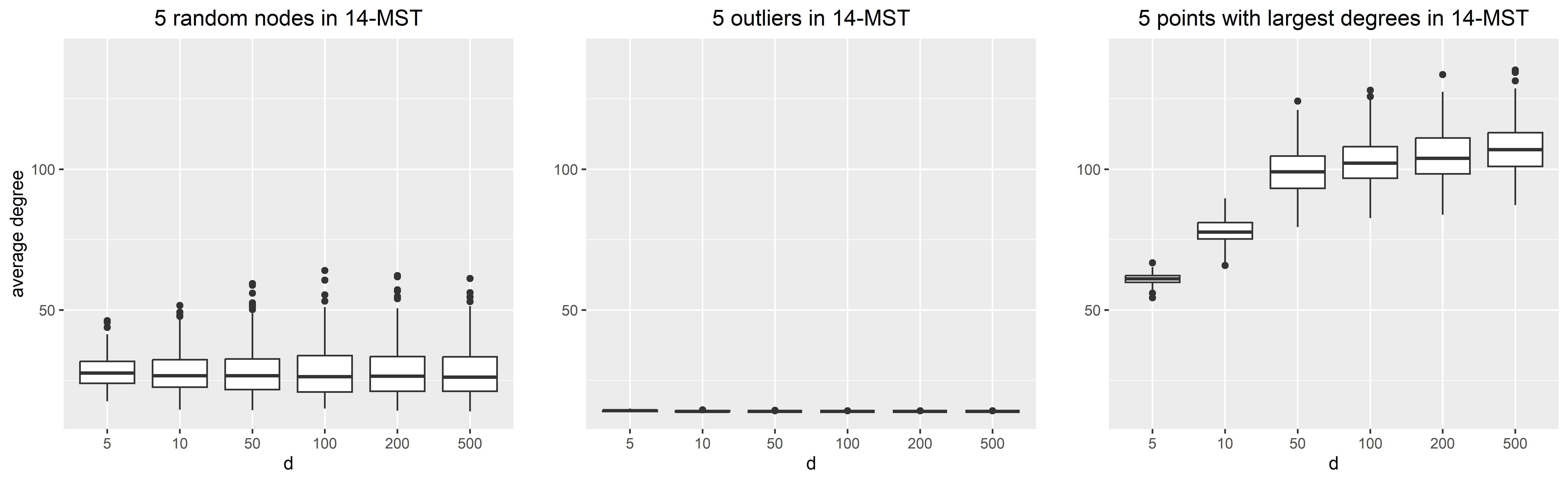
Figure 18: The average degrees of selected points under different dimensions in $K$-MST.

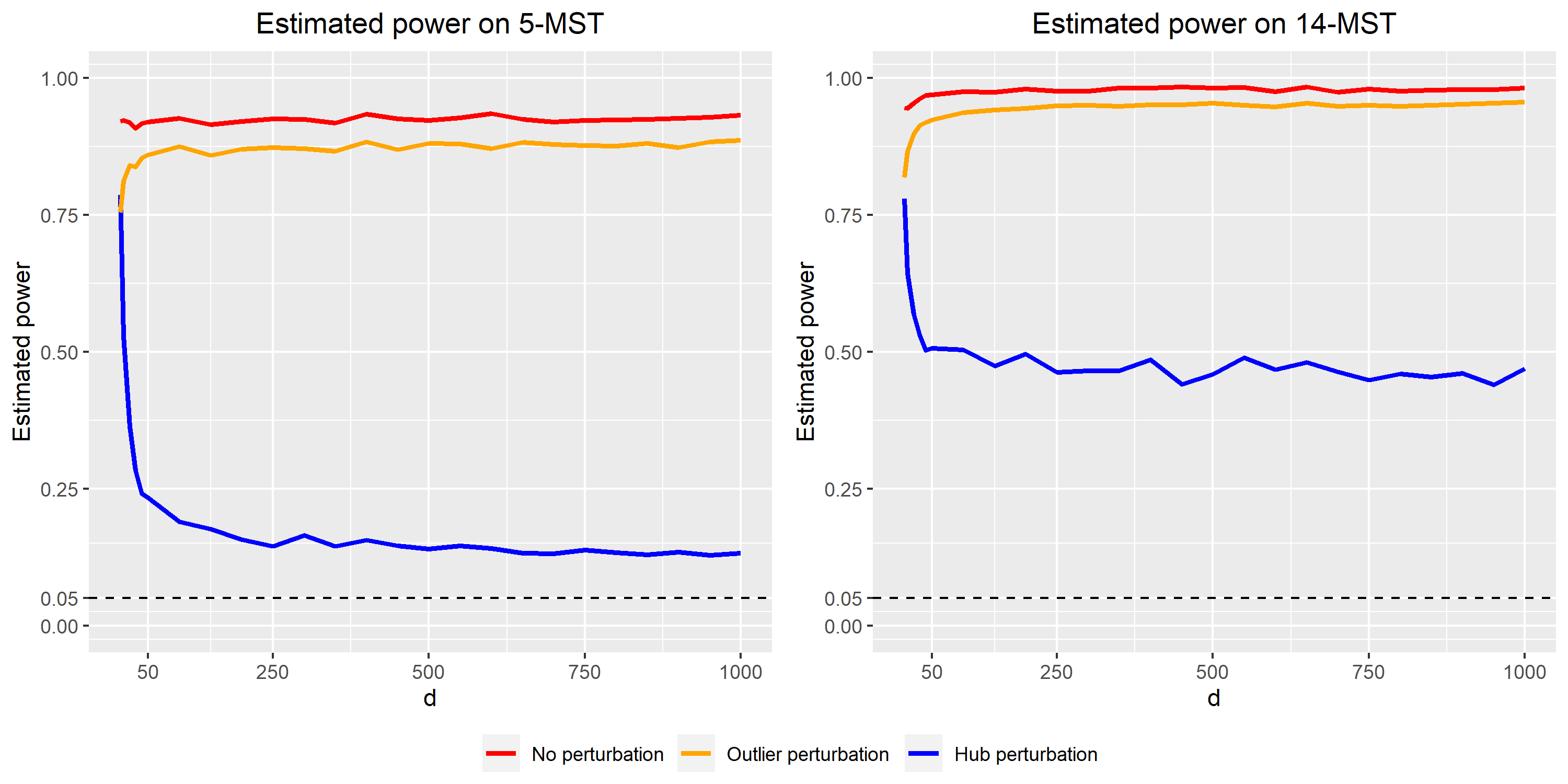
Figure 19: Estimated power of GET on the $5$-MST and the $14$-MST under different dimensions.

Appendix B Estimated power and accuracy in the change-point detection analysis

Estimated power and accuracy of change-point detection numeric study under Setting 2 and 3 are plotted in Figure 20 and 21.

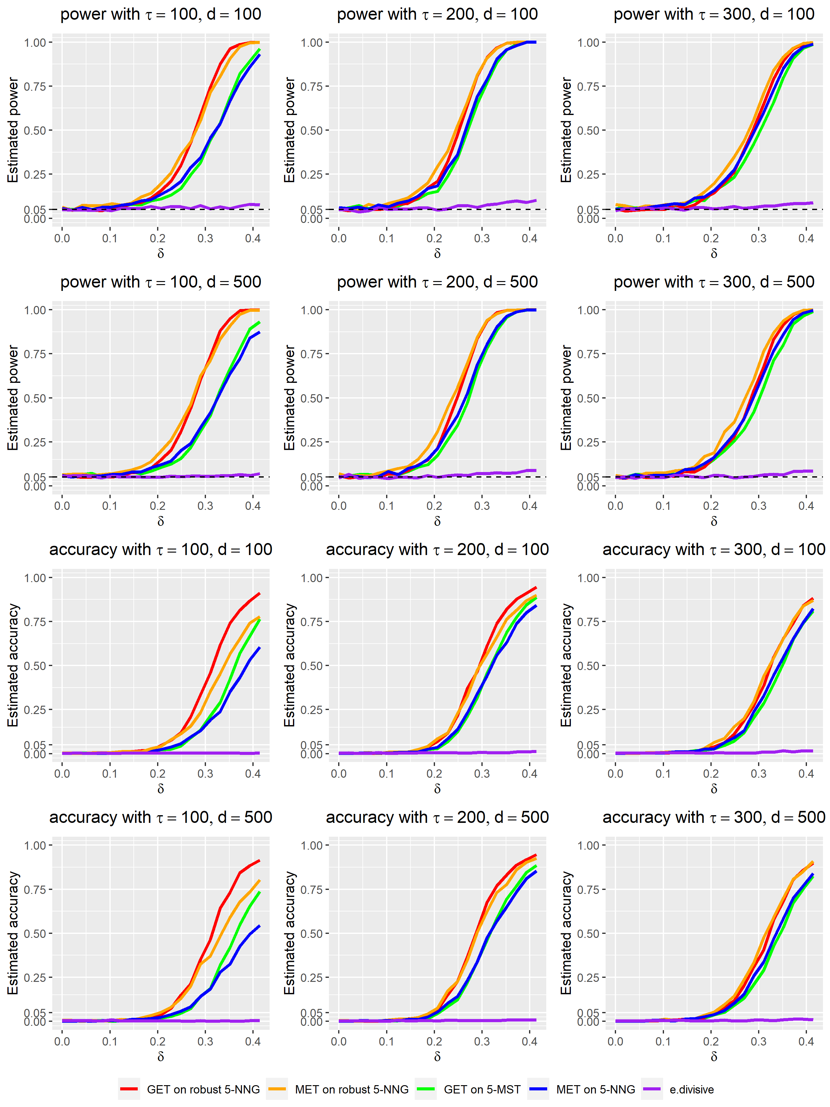
Figure 20: Estimated power and accuracy of change-point detection methods for Setting 2.

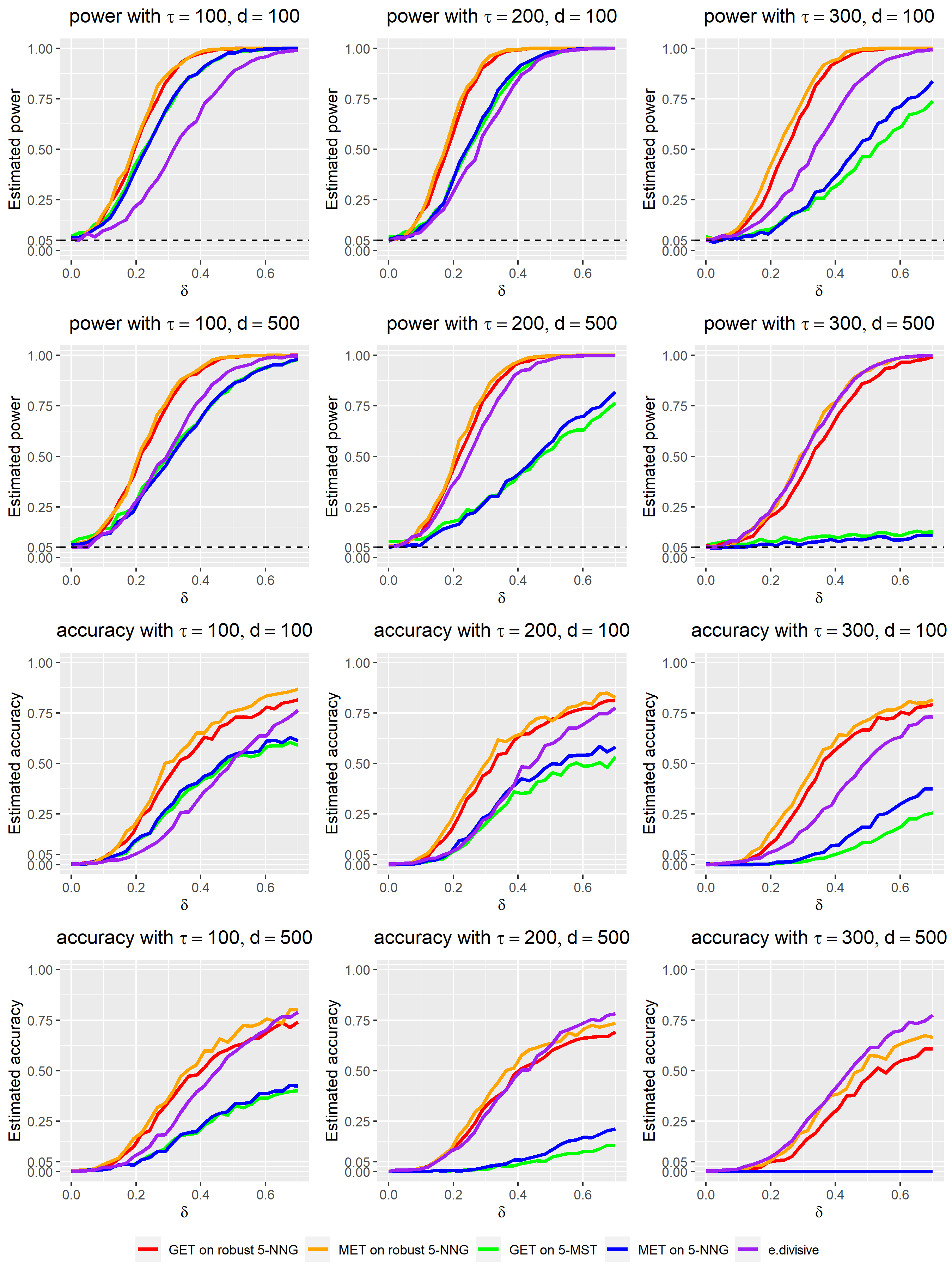
Figure 21: Estimated power and accuracy of change-point detection methods for Setting 3.

References

- Beckmann et al. [2021] N. D. Beckmann, P. H. Comella, E. Cheng, L. Lepow, A. G. Beckmann, S. R. Tyler, K. Mouskas, N. W. Simons, G. E. Hoffman, N. J. Francoeur, et al. Downregulation of exhausted cytotoxic t cells in gene expression networks of multisystem inflammatory syndrome in children. Nature communications, 12(1):1–15, 2021.
- Biswas et al. [2014] M. Biswas, M. Mukhopadhyay, and A. K. Ghosh. A distribution-free two-sample run test applicable to high-dimensional data. Biometrika, 101(4):913–926, 2014.
- Bullmore and Sporns [2009] E. Bullmore and O. Sporns. Complex brain networks: graph theoretical analysis of structural and functional systems. Nature reviews neuroscience, 10(3):186–198, 2009.
- Chen and Friedman [2017] H. Chen and J. H. Friedman. A new graph-based two-sample test for multivariate and object data. Journal of the American statistical association, 112(517):397–409, 2017.
- Chen et al. [2018] H. Chen, X. Chen, and Y. Su. A weighted edge-count two-sample test for multivariate and object data. Journal of the American Statistical Association, 113(523):1146–1155, 2018.
- Chu and Chen [2019] L. Chu and H. Chen. Asymptotic distribution-free change-point detection for multivariate and non-euclidean data. The Annals of Statistics, 47(1):382–414, 2019.
- Deb and Sen [2021] N. Deb and B. Sen. Multivariate rank-based distribution-free nonparametric testing using measure transportation. Journal of the American Statistical Association, pages 1–16, 2021.
- Feigenson et al. [2014] K. A. Feigenson, M. A. Gara, M. W. Roché, and S. M. Silverstein. Is disorganization a feature of schizophrenia or a modifying influence: evidence of covariation of perceptual and cognitive organization in a non-patient sample. Psychiatry research, 217(1-2):1–8, 2014.
- Friedman and Rafsky [1979] J. H. Friedman and L. C. Rafsky. Multivariate generalizations of the wald-wolfowitz and smirnov two-sample tests. The Annals of Statistics, pages 697–717, 1979.
- Gretton et al. [2008] A. Gretton, K. Borgwardt, M. J. Rasch, B. Scholkopf, and A. J. Smola. A kernel method for the two-sample problem. arXiv preprint arXiv:0805.2368, 2008.
- Gretton et al. [2012a] A. Gretton, K. M. Borgwardt, M. J. Rasch, B. Schölkopf, and A. Smola. A kernel two-sample test. The Journal of Machine Learning Research, 13(1):723–773, 2012a.
- Gretton et al. [2012b] A. Gretton, D. Sejdinovic, H. Strathmann, S. Balakrishnan, M. Pontil, K. Fukumizu, and B. K. Sriperumbudur. Optimal kernel choice for large-scale two-sample tests. Advances in neural information processing systems, 25, 2012b.
- Henze [1988] N. Henze. A multivariate two-sample test based on the number of nearest neighbor type coincidences. The Annals of Statistics, 16(2):772–783, 1988.
- James and Matteson [2013] N. A. James and D. S. Matteson. ecp: An r package for nonparametric multiple change point analysis of multivariate data. arXiv preprint arXiv:1309.3295, 2013.
- Koboldt et al. [2012] D. Koboldt, R. Fulton, M. McLellan, H. Schmidt, J. Kalicki-Veizer, J. McMichael, L. Fulton, D. Dooling, L. Ding, E. Mardis, et al. Comprehensive molecular portraits of human breast tumours. Nature, 490(7418):61–70, 2012.
- Li et al. [2020] H. Li, A. Aue, D. Paul, J. Peng, and P. Wang. An adaptable generalization of hotelling’s test in high dimension. The Annals of Statistics, 48(3):1815–1847, 2020.
- Liu and Chen [2022] Y.-W. Liu and H. Chen. A fast and efficient change-point detection framework based on approximate -nearest neighbor graphs. IEEE Transactions on Signal Processing, 70:1976–1986, 2022.
- Matteson and James [2014] D. S. Matteson and N. A. James. A nonparametric approach for multiple change point analysis of multivariate data. Journal of the American Statistical Association, 109(505):334–345, 2014.
- Pan et al. [2018] W. Pan, Y. Tian, X. Wang, and H. Zhang. Ball divergence: nonparametric two sample test. Annals of statistics, 46(3):1109, 2018.
- Radovanovic et al. [2010] M. Radovanovic, A. Nanopoulos, and M. Ivanovic. Hubs in space: Popular nearest neighbors in high-dimensional data. Journal of Machine Learning Research, 11(sept):2487–2531, 2010.
- Rosenbaum [2005] P. R. Rosenbaum. An exact distribution-free test comparing two multivariate distributions based on adjacency. Journal of the Royal Statistical Society: Series B (Statistical Methodology), 67(4):515–530, 2005.
- Schilling [1986] M. F. Schilling. Multivariate two-sample tests based on nearest neighbors. Journal of the American Statistical Association, 81(395):799–806, 1986.
- Song and Chen [2022] H. Song and H. Chen. Asymptotic distribution-free changepoint detection for data with repeated observations. Biometrika, 109(3):783–798, 2022.
- Zhu and Chen [2021] Y. Zhu and H. Chen. Limiting distributions of graph-based test statistics on sparse and dense graphs. arXiv preprint arXiv:2108.07446, 2021.