The Marginal Value of Momentum
for Small Learning Rate SGD

Abstract

Momentum is known to accelerate the convergence of gradient descent in strongly convex settings without stochastic gradient noise. In stochastic optimization, such as training neural networks, folklore suggests that momentum may help deep learning optimization by reducing the variance of the stochastic gradient update, but previous theoretical analyses do not find momentum to offer any provable acceleration. Theoretical results in this paper clarify the role of momentum in stochastic settings where the learning rate is small and gradient noise is the dominant source of instability, suggesting that SGD with and without momentum behave similarly in the short and long time horizons. Experiments show that momentum indeed has limited benefits for both optimization and generalization in practical training regimes where the optimal learning rate is not very large, including small- to medium-batch training from scratch on ImageNet and fine-tuning language models on downstream tasks.

1 Introduction

In modern deep learning, it is standard to combine stochastic gradient methods with heavy-ball momentum, or momentum for short, to enable a more stable and efficient training of neural networks (Sutskever et al., 2013). The simplest form is Stochastic Gradient Descent with Momentum (SGDM). SGDM aims to minimize the training loss $\mathcal{L}({\bm{x}})$ given a noisy gradient oracle $\mathcal{G}({\bm{x}})$, which is usually realized by evaluating the gradient at a randomly sampled mini-batch from the training set. Specifically, let $\gamma,\beta$ be the learning rate and momentum coefficient, then SGDM can be stated as follows:

$${\bm{g}}_{k}\sim\mathcal{G}({\bm{x}}_{k}),\qquad{\bm{m}}_{k+1}=\beta{\bm{m}}_{k}+{\bm{g}}_{k},\qquad{\bm{x}}_{k+1}={\bm{x}}_{k}-\gamma{\bm{m}}_{k+1},$$ (1)

where ${\bm{g}}_{k},{\bm{m}}_{k},{\bm{x}}_{k}$ are the gradient, momentum buffer, and parameter vector at step $k$. See Definition 3.3 for its formal formulation.

For typical choices of $\beta\in(0,1)$, the momentum buffer can be interpreted as an exponential moving average of past gradients, i.e., ${\bm{m}}_{k}=\sum_{j=0}^{k}\beta^{k-j}{\bm{g}}_{j}$. Based on this interpretation, Polyak (1964, 1987); Rumelhart et al. (1987) argued that momentum is able to cancel out oscillations along high-curvature directions and add up contributions along low-curvature directions. More concretely, for strongly convex functions without any noise in gradient estimates, Polyak (1964, 1987) showed that adding momentum can stabilize the optimization process even when the learning rate is so large that can make vanilla gradient descent diverge, and thus momentum accelerates the convergence to minimizers by allowing using a larger learning rate.

In deep learning, however, the random sampling of mini-batches inevitably introduces a large amount of stochastic gradient noise. In addition to the high-curvature directions causing the parameter to oscillate back and forth, this large gradient noise can further destabilize training and hinder the use of large learning rates. Given the aforementioned convergence results that solely analyze the noiseless case, it remains unclear whether momentum can likewise stabilize the stochastic optimization process in deep learning. Still, it is intuitive that averaging past stochastic gradients could reduce the variance of the noise in the updates, as long as the parameter does not move drastically fast at each step. Several prior studies indeed cited this reduction of noise in SGDM as a possible advantage that may encourage a more rapid decrease in loss (Bottou et al., 2018; Defazio, 2020; You et al., 2020). To approach this more rigorously, Cutkosky and Orabona (2019) proposed a variant of SGDM that provably accelerates training by leveraging the reduced variance in the updates. They further speculated that the advantage of the original SGDM might be related in some way.

Nevertheless, for SGDM without any modification, past theoretical analyses in the stochastic optimization of convex and non-convex functions usually conclude with a comparable convergence rate as vanilla SGD, rather than a faster one (Yan et al., 2018; Yu et al., 2019; Liu et al., 2020; Sebbouh et al., 2021; Li et al., 2022a). Besides, there also exist simple and concrete instances of convex optimization where momentum does not speed up the convergence rate of SGD, even though it is possible to optimize faster with some variants of SGDM (Kidambi et al., 2018). Despite these failures in theory, it has been empirically confirmed that SGDM continues to stabilize large learning rate training even in the presence of gradient noise. Kidambi et al. (2018); Shallue et al. (2019); Smith et al. (2020) observed that for large-batch training, SGDM can successfully perform training with a large learning rate, in which regime vanilla SGD may exhibit instability that degrades the training speed and generalization. This naturally raises the following question on the true role of momentum:

Is the noise reduction in the updates of SGDM really beneficial to training neural networks?

To address this question, our paper delves into the training regime where the learning rate is small enough to prevent oscillations along high-curvature directions, yet the gradient noise is large enough to induce instability. This setting enables us to concentrate exclusively on the interplay between momentum and gradient noise. More importantly, this training regime is of practical significance as in many situations, such as small-batch training from scratch or fine-tuning a pre-trained model, the optimal learning rate is indeed relatively small (Liu et al., 2019; Malladi et al., 2023).

Main Contributions.

In this paper, we present analyses of the training trajectories of SGD with and without momentum, in the regime of small learning rate. We provide theoretical justifications of a long-held belief that SGDM with learning rate $\gamma$ and momentum $\beta$ performs comparably to SGD with learning rate $\frac{\gamma}{1-\beta}$ (Tugay and Tanik, 1989; Orr, 1996; Qian, 1999; Yuan et al., 2016; Smith et al., 2020). This finding offers negative evidence for the usefulness of noise reduction in momentum.

More specifically, given a run of SGDM, we show that vanilla SGD can closely track its trajectory in the following two regimes with different time horizon:

Regime I.

Training with SGD and SGDM for $O(1/\eta)$ steps with gradient noise covariance inversely scaled with $\eta$ leads to the same SDE approximation. Scaling down batch-size with the Linear Scaling Rule (Goyal et al., 2017) falls into this regime. See Section 4.

Regime II.

Training with SGD and SGDM for $O(1/\eta^{2})$ steps, where the loss is mostly zero but the gradient noise induces certain drift and diffusion on the minimizer manifold that may benefit generalization, also leads to the same SDE approximation. See Section 5.

Our results improve over previous analysis Yuan et al. (2016); Liu et al. (2018) on the approximation of SGDM by avoiding underestimating the role of noise when scaling down the learning rate, and provide rigorous theoretical supports to the scaling claims in Smith et al. (2020); Cowsik et al. (2022).

In Section 6, we show empirically that momentum indeed has limited benefits for both optimization and generalization in practical training regimes with optimal learning rate being not very large, including small- to medium-batch training from scratch on ImageNet and fine-tuning RoBERTa-large on downstream tasks. We also look into a large-batch training case on CIFAR-10 where SGDM indeed outperforms vanilla SGD, and show that reducing training instability induced by high curvature by running an SDE simulation method called SVAG (Li et al., 2021a) can shrink or eliminate the performance gain.

Finally, we highlight that our results can also have practical significance beyond just understanding the role of momentum. In recent years, the GPU memory capacity sometimes becomes a bottleneck in training large models. As the momentum buffer costs as expensive as storing the entire model, it has raised much interest in when it is safe to remove momentum (Shazeer and Stern, 2018). Our work sheds light on this question by formally proving that momentum only provides marginal values in small learning rate SGD. Furthermore, our results imply that within reasonable range of scales the final performance is insensitive to the momentum hyperparametrization, thereby provide support to save the effort in the extensive hyperparameter grid search.

2 Related Works

The role of momentum in optimization. Besides the works mentioned in the introduction, there are many other works discussing the role of momentum. The accelerating effect of some variants of momentum has been observed in settings such as convex optimization (Kidambi et al., 2018) and linear regression (Jain et al., 2018) with parametrizations specific to their settings. Smith (2018) pointed out that momentum can help stabilize training, but the optimal choice of momentum is closed related to the choice of learning rate. Arnold et al. (2019) argued using a quadratic example that momentum might no reduce variance as the gradient noise in each would actually be carried over to future iterates due to momentum. Tondji et al. (2021) showed that the application of a multi-momentum strategy can achieve variance reduction in deep learning. Plattner (2022) empirically established that momentum enlarges the learning rate while not contributing to a boost in performance.

Defazio (2020) proposed a stochastic primal averaging formulation for SGDM which facilitates a Lyapunov analysis for SGDM, and one particular insight from their analysis is that momentum may help reduce noise in the early stage of training but is no longer helpful when the iterates are close to local minima. Xie et al. (2021) showed that under SDE approximation, the posterior of SGDM is the same as that of SGD. Jelassi and Li (2022) proved the generalization benefit of momentum in GD in a specific setting of binary classification, by showing that GD+M is able to learn small margin data from the historical gradients in the momentum. A stronger implicit regularization effect of momentum in GD is also proved in Ghosh et al. (2023).

Convergence of momentum methods. There are many works analyzing the convergence of momentum methods, yet it is often the case that momentum appears as a technical barrier rather than leading to faster convergence rates. Yu et al. (2019) showed that distributed SGDM can achieve the same linear speedup as ditributed SGD in the setting of distributed non-convex optimization. Yan et al. (2018) provided a unified analysis of SGD, SGDM and stochastic Nestrov’s accelerated gradient descent for non-convex optimization, showing that the gradient norm converges in the same rate for the three variants. They also argued that momentum helps generalization from the lens of stability analysis for finite number of iterates, when the loss function is Lipschitz. Under the formulation of quasi-hyperbolic momentum (Ma and Yarats, 2019), Gitman et al. (2019) proposed another unified analysis for momentum methods, in terms of the asymptotic and local convergence as well as the stability. Liu et al. (2020) proved that SGDM converges as fast as SGD for strongly convex and non-convex objectives, and their analysis achieved improved convergence bound without the bounded gradient assumption. Using a iterate-averaging formulation of SGDM, Sebbouh et al. (2021) proved last-iterate convergence of SGDM in both convex and non-convex settings. Later in Li et al. (2022a), it is shown that constant momentum can lead to suboptimal last-iterate convergence rate and increasing momentum resolves the issue. Smith (2018); Liu et al. (2018) provided evidence that momentum helps escape saddle points but hurts the final convergence without parameter annealing.

Characterizing implicit bias near manifold of local minimizers A recent line of work has studied the implicit bias induced by gradient noise in SGD-type algorithms, when iterates are close to some manifold of local minimizers (Blanc et al., 2020; Damian et al., 2021; Li et al., 2021b). In particular, Li et al. (2021b) developed a framework for describing the dynamics of SGD via a slow SDE on the manifold of local minimizers in the regime of small learning rate. The idea is to rescale the time by $1/\eta^{2}$ times to reveal the relatively slow movement of the iterates along the manifold. Similar methodology has become a powerful tool for analyzing algorithmic implicit bias and has been extended to many other settings, including SGD/GD for models with normalization layers (Lyu et al., 2022; Li et al., 2022b), GD in the edge of stability regime (Arora et al., 2022), Local SGD (Gu et al., 2023), sharpness-aware minimization (Wen et al., 2022), and pre-training for language models (Liu et al., 2022). Notably, Cowsik et al. (2022) utilized the similar idea to study the slow SDE of SGDM study the optimal scale of the momentum parameter with respect to the learning rate, which has a focus different from our paper.

3 Preliminaries

Consider optimizing a loss function $\mathcal{L}=\frac{1}{\Xi}\sum_{i=1}^{\Xi}\mathcal{L}_{i}$ where $\mathcal{L}_{i}:\mathbb{R}^{d}\to\mathbb{R}$ corresponds to the loss on the $i$-th sample. We use ${\bm{\theta}}$ to indicate parameters along a general trajectory. In each step, we sample a random minibatch $\mathcal{B}\subseteq[\Xi]$, and compute the gradient of the minibatch loss $\mathcal{L}_{\mathcal{B}}=\frac{1}{|\mathcal{B}|}\sum_{i\in\mathcal{B}}\mathcal{L}_{i}$ to get the following noisy estimate of $\nabla\mathcal{L}(\bm{\theta})$, i.e., $\nabla\mathcal{L}_{\mathcal{B}}(\bm{\theta})=\frac{1}{|\mathcal{B}|}\sum_{i\in\mathcal{B}}\nabla\mathcal{L}_{i}(\bm{\theta})$. It is easy to check that the noise covariance matrix of $\nabla\mathcal{L}_{\mathcal{B}}(\bm{\theta})$, namely $\mathbb{E}_{\mathcal{B}}(\nabla\mathcal{L}_{\mathcal{B}}({\bm{\theta}})-\nabla\mathcal{L}({\bm{\theta}}))(\nabla\mathcal{L}_{\mathcal{B}}({\bm{\theta}})-\nabla\mathcal{L}({\bm{\theta}}))^{\top}$, scales proportionally to $\frac{1}{|\mathcal{B}|}$. Motivated by this, Malladi et al. (2022) abstracts $\nabla\mathcal{L}_{\mathcal{B}}(\bm{\theta})$ as sampled from a noisy gradient oracle where the noise covariance depends on a scale parameter.

Definition 3.1 (NGOS, Malladi et al. (2022)).

A Noisy Gradient Oracle with Scale Parameter (NGOS) is characterized by a tuple $\mathcal{G}_{\sigma}=(\mathcal{L},{\bm{\Sigma}},\mathcal{Z}_{\sigma})$. For a scale parameter $\sigma>0$, $\mathcal{G}_{\sigma}$ takes as input ${\bm{\theta}}$ and returns ${\bm{g}}=\nabla\mathcal{L}({\bm{\theta}})+\sigma{\bm{v}}$, where $\nabla\mathcal{L}({\bm{\theta}})$ is the gradient of $\mathcal{L}$ at ${\bm{\theta}}$, ${\bm{v}}$ is the gradient noise drawn from the probability distribution $\mathcal{Z}_{\sigma}({\bm{\theta}})$ with mean zero and covariance matrix ${\bm{\Sigma}}({\bm{\theta}})$. The matrix ${\bm{\Sigma}}({\bm{\theta}})$ is independent of the noise scale $\sigma$. We use $\mathcal{G}_{\sigma}({\bm{\theta}})$ to denote the distribution of ${\bm{g}}$ given $\sigma$ and ${\bm{\theta}}$.

In our work we invoke NGOS with different $\sigma$ for different magnitudes of the learning rate, so that we can augment the noise level when the learning rates are set smaller. The scaling is discussed after Lemma 3.4. We now instantiate the SGD and SGDM trajectories under this noise oracle.

Definition 3.2 (Vanilla SGD).

Given a stochastic gradient ${\bm{g}}_{k}\sim\mathcal{G}_{\sigma}({\bm{z}}_{k})$, minibatch SGD with the learning rate schedule $\{\bar{\eta}_{k}\}$ updates the parameters ${\bm{z}}_{k}\in\mathbb{R}^{d}$ from initialization ${\bm{z}}_{0}$ as

$${\bm{z}}_{k+1}={\bm{z}}_{k}-\bar{\eta}_{k}{\bm{g}}_{k}.$$ (2)

Definition 3.3 (SGD with momentum/SGDM).

Given a stochastic gradient ${\bm{g}}_{k}\sim\mathcal{G}_{\sigma}({\bm{x}}_{k})$ minibatch SGDM with the hyperparameter schedule $\{(\eta_{k},\beta_{k})\}$, where $\beta_{k}\in(0,1)$, updates the parameters ${\bm{x}}_{k}\in\mathbb{R}^{d}$ from $({\bm{m}}_{0},{\bm{x}}_{0})$ as

$${\bm{m}}_{k+1}=\beta_{k}{\bm{m}}_{k}+(1-\beta_{k}){\bm{g}}_{k},\qquad{\bm{x}}_{k+1}={\bm{x}}_{k}-\eta_{k}{\bm{m}}_{k+1}.$$ (3)

Notice that the formulation SGDM in Definition 3.3 is different from (1). An easy conversion is given by rewriting Equation 3 as:

$${\bm{x}}_{k+1}={\bm{x}}_{k}-\eta_{k}(1-\beta_{k}){\bm{g}}_{k}+\beta_{k}\frac{\eta_{k}}{\eta_{k-1}}({\bm{x}}_{k}-{\bm{x}}_{k-1}).$$

Then setting $\eta_{k}=\frac{\gamma}{1-\beta}$ and $\beta_{k}=\beta$ recovers the form of (1). $\eta_{k}$ is arguably a more natural parameterization that is under the same scale of the learning rates of SGD for comparison.

Modeling the gradient noise as an NGOS gives us the flexibility to scale the noise in our theoretical setting to make the effect of noise non-vanishing in small learning rate training. This is motivated by the following variant of the standard descent lemma, which highlights noise-induced and curvature-induced factors that prevent the loss to decrease:

Lemma 3.4 (Descent Lemma).

For the SGD updates ${\bm{z}}_{k}$, the expected change in loss per step is

$$\mathbb{E}[\mathcal{L}({\bm{z}}_{k+1})|{\bm{z}}_{k}]-\mathcal{L}({\bm{z}}_{k})=$$

$$\qquad\underbrace{-\eta\left\|\nabla\mathcal{L}({\bm{z}}_{k})\right\|^{2}}_{\text{descent force}}+\underbrace{\frac{1}{2}(\sigma\eta)^{2}\mathop{\mathrm{tr}}((\nabla^{2}\mathcal{L}){\bm{\Sigma}}({\bm{z}}_{k}))}_{\text{noise-induced}}+\underbrace{\frac{1}{2}\eta^{2}(\nabla\mathcal{L}^{\top}(\nabla^{2}\mathcal{L})\nabla\mathcal{L}({\bm{z}}_{k}))}_{\text{curvature-induced}}+o(\eta^{2},(\sigma\eta)^{2}).$$

When scaling down the learning rate, the descent force scales with $O(\eta)$ and the noise-induced impact scales with $O(\sigma^{2}\eta^{2})$, therefore we need to set $\sigma=1/\sqrt{\eta}$ to ensure that noises maintain the same scale of effect across different scales of $\eta$. When $\eta\to 0$ under this scaling, if we consider running the updates for $O(1/\eta)$ steps, only the curvature-induced impact is vanishing among the three.

4 Weak Approximation of SGDM by SGD in $O(1/\eta)$ Steps

In the following two sections, we will present our main theoretical results on SGDM with small learning rate. In this section, we show that in $O(1/\eta)$ steps, SGD approximates SGDM in the sense of Definition 4.4. The next section characterizes SGDM over a longer training time (i.e., $O(1/\eta^{2})$ steps) to characterize generalization and finds that the limiting dynamics of SGDM and SGD coincide.

4.1 A Warm Up Example: The Variance Reduction Effect of Momentum

Intuitively, momentum makes the SGD update direction less noisy by averaging past stochastic gradients, which seems at first glance to contradict our result that the distribution of SGD and SGDM at any time point are approximately the same. However, the apparent discrepancy can be explained by the following effect: by carrying the noise at a step to subsequent steps, the updates of SGDM have long-range correlations.

For instance, we consider the case where the stochastic gradients are i.i.d. gaussian as ${\bm{g}}_{k}\sim\mathcal{N}({\bm{c}},{\bm{I}})$ for a constant vector ${\bm{c}}$. We compare SGD and SGDM trajectories with hyperparameter $\eta_{k}=\eta$ and $\beta_{k}=\beta$, and initialization ${\bm{z}}_{0}={\bm{x}}_{0}$ and ${\bm{m}}_{0}\sim\mathcal{N}({\bm{c}},\frac{1-\beta}{1+\beta}{\bm{I}})$. The single-step updates are

$${\bm{z}}_{k+1}-{\bm{z}}_{k} =-\eta{\bm{g}}_{k}\sim\mathcal{N}(-\eta{\bm{c}},\eta^{2}{\bm{I}}).$$

$${\bm{x}}_{k+1}-{\bm{x}}_{k} =-\eta{\bm{m}}_{k+1}=-\eta(\beta^{k+1}{\bm{m}}_{0}+\sum_{s=0}^{k}\beta^{k-s}(1-\beta){\bm{g}}_{s})\sim\mathcal{N}(-\eta{\bm{c}},\frac{1-\beta}{1+\beta}\eta^{2}{\bm{I}}).$$

Therefore, the variance of each single-step update is reduced by a factor of $\frac{1-\beta}{1+\beta}$, which implies larger momentum generates a smoother trajectory. Furthermore, measuring the turbulence over a fixed interval via the path length $\sum_{k}\left\|{\bm{z}}_{k+1}-{\bm{z}}_{k}\right\|_{2}$ or the loss variation $\sum_{k}|\mathcal{L}({\bm{z}}_{k+1})-\mathcal{L}({\bm{z}}_{k})|$ indeed suggests that adding momentum smooths the path.

However, we are usually more interested in tracking the final loss distributions induced by each trajectory. The distributions of after $k$ steps are

$${\bm{z}}_{k} \sim\mathcal{N}({\bm{z}}_{0}-k\eta{\bm{c}},k\eta^{2}{\bm{I}});$$

$${\bm{x}}_{k} ={\bm{z}}_{0}-\eta\beta\frac{1-\beta^{k}}{1-\beta}{\bm{m}}_{0}-\eta\sum_{s=0}^{k-1}(1-\beta^{k-s}){\bm{g}}_{s}\sim\mathcal{N}\bigg{(}{\bm{z}}_{0}-k\eta{\bm{c}},k\eta^{2}{\bm{I}}-2\beta\eta^{2}\frac{1-\beta^{k}}{1-\beta^{2}}{\bm{I}}\bigg{)}.$$

Notice that the variance of the final endpoint is only different by $|2\beta\eta^{2}\frac{1-\beta^{k}}{1-\beta^{2}}|\leq\frac{2\eta^{2}}{1-\beta}$, which is bounded regardless of $k$. The variance is increased at rate $\eta^{2}$ per step, which is significantly larger than the per step update variance $\frac{1-\beta}{1+\beta}\eta^{2}$. As such, the turbulence of the path may not faithfully reflect the true stochasticity of the iterates.

4.2 Main Results on Weak Approximations of SGDM

We study the setting where the magnitude of the hyperparameters are controlled. Let $\eta$ be the scale of the learning rate so that $\eta_{k}=O(\eta)$. Furthermore, we set an index $\alpha\geq 0$ so that the decay rate of the momentum is controlled as $1-\beta_{k}=O(\eta^{\alpha})$. $\alpha=0$ corresponds to a constant decay schedule while $\alpha>0$ corresponds to a schedule where we make $\beta_{k}$ closer to $1$ when the learning rates are getting smaller. More formally, we associate a hyperparameter schedule $(\eta_{k}^{\eta},\beta_{k}^{\eta})$ for each scale $\eta$ such that the following assumption is satisfied.

Definition 4.1 (Hyperparameter Schedule Scaling).

A family of hyperparameter schedules $\{\eta^{(n)}_{k},\beta^{(n)}_{k}\}_{k\geq 1}$ is scaled by $\eta^{(n)}$ with index $\alpha$ if there are constants $\eta_{\max},\lambda_{\min}$ and $\lambda_{\max}$ independent of $n$, such that for all $n$

$$0\leq\frac{\eta^{(n)}_{k}}{\eta^{(n)}}<\eta_{\max},\quad 0<\lambda_{\min}\leq\frac{1-\beta^{(n)}_{k}}{(\eta^{(n)})^{\alpha}}\leq\lambda_{\max}<1.$$

We need some boundedness of the initial momentum for the SGDM trajectory to start safely.

Assumption 4.2 (Boundedness of the Initial Momentum).

For each $m\geq 1$, there is constant $C_{m}\geq 0$ that $\mathbb{E}(\left\|{\bm{m}}_{0}\right\|_{2}^{m})\leq C_{m}$;

Following Malladi et al. (2022), we further assume that the NGOS satisfies the below conditions, which make the trajectory amenable to analysis. We say a function $g(\bm{x}):{\mathbb{R}}^{d}\to{\mathbb{R}}^{m}$ has polynomial growth if there are constants $k_{1},k_{2}>0$ such that $\left\|g(\bm{x})\right\|_{2}\leq k_{1}(1+\left\|\bm{x}\right\|_{2}^{k_{2}})$, $\forall\bm{x}\in\mathbb{R}^{d}$.

Assumption 4.3.

The NGOS $\mathcal{G}_{\sigma}=(\mathcal{L},{\bm{\Sigma}},\mathcal{Z}_{\sigma})$ satisfies the following conditions.

1. Well-Behaved: $\nabla\mathcal{L}$ is Lipschitz and $\mathcal{C}^{\infty}$-smooth; ${\bm{\Sigma}}^{1/2}$ is bounded, Lipschitz, and $\mathcal{C}^{\infty}$-smooth; all partial derivatives of $\nabla\mathcal{L}$ and ${\bm{\Sigma}}^{1/2}$ up to and including the third order have polynomial growth.

2. Bounded Moments: For all integers $m\geq 1$ and all noise scale parameters $\sigma$, there exists a constant $C_{2m}$ (independent of $\sigma$) such that $(\mathbb{E}_{{\bm{v}}\sim\mathcal{Z}_{\sigma}({\bm{\theta}})}[\left\|{\bm{v}}\right\|_{2}^{2m}])^{\frac{1}{2m}}\leq C_{2m}(1+\left\|{\bm{\theta}}\right\|_{2})$, $\forall{\bm{\theta}}\in\mathbb{R}^{d}$.

Besides, to rigorously discuss the closeness between dynamics of different algorithms, we introduce the following notion of approximation between two discrete trajectories, inspired by (Li et al., 2019).

Definition 4.4 (Order-$\gamma$ Weak Approximation).

Two families of discrete trajectories ${\bm{x}}^{\eta}_{k}$ and ${\bm{y}}^{\eta}_{k}$ are weak approximations of each other, if there is $\eta_{\text{thr}}>0$ that for any $T>0$, any function $h$ of polynomial growth, and any $\eta\leq\eta_{\text{thr}}$, there is a constant $C_{h,T}$ independent of $\eta$ such that,

$$\max_{k=0,...,\lfloor T/\eta\rfloor}|\mathbb{E}h({\bm{x}}^{\eta}_{k})-\mathbb{E}h({\bm{y}}^{\eta}_{k})|\leq C_{h,T}\cdot\eta^{\gamma}.$$

Weak approximation implies that ${\bm{x}}_{k}^{\eta}$ and ${\bm{y}}_{k}^{\eta}$ have similar distributions at any step $k$, and specifically in the deep learning setting it implies that both training (or testing) curves are similar. Given the above definitions, we are ready to establish our main result.

Theorem 4.5 (Weak Approximation of SGDM by SGD).

Fix the initial point ${\bm{x}}_{0}$ , $\alpha\in[0,1)$, and an NGOS satisfying Assumption 4.3. Consider the SGDM update ${\bm{x}}^{\eta}_{k}$ with hyperparameter schedule $\{\eta_{k},\beta_{k}\}_{k\geq 1}$ scaled by $\eta$ with index $\alpha$, noise scaling $\sigma\leq\eta^{-1/2}$ and initialization $({\bm{m}}_{0},{\bm{x}}_{0})$ satisfying Assumption 4.2, then ${\bm{x}}^{\eta}_{k}$ is an order-$(1-\alpha)/2$ weak approximation (Definition 4.4) of the trajectories ${\bm{z}}^{\eta}_{k}$ with initialization ${\bm{z}}^{\eta}_{0}={\bm{x}}_{0}$, noise scaling $\sigma$ and an averaged learning rate schedule $(\bar{\eta}_{k}=\sum_{s=k}^{\infty}\eta_{s}\prod_{\tau=k+1}^{s}\beta_{\tau}(1-\beta_{k})).$ Specifically, for a constant schedule where $(\eta_{k}=\eta,\beta_{k}=\beta)$ and $\bar{\eta}_{k}=\eta$, SGD and SGDM with the same learning rate weakly approximate each other.

The theorem shows that when the learning rate have a small scale $\eta$, then the trajectory of SGDM and SGD will be close in distribution over $O(1/\eta)$ steps, when the gradient noise is amplified at a scale no more than $\eta^{-1/2}$. Specifically when we consider the limit $\eta\to 0$, then the trajectories of SGDM and SGD will have the same distribution. Following the idea of Stochastic Modified Equations (Li et al., 2019), the limiting distribution can be described by the law of the solution ${\bm{X}}_{t}$ to an SDE $\textup{{d}}{\bm{X}}_{t}=-\lambda_{t}\nabla\mathcal{L}({\bm{X}}_{t})\textup{{d}}t+\lambda_{t}{\bm{\Sigma}}^{1/2}({\bm{X}}_{t})\textup{{d}}{\bm{W}}_{t}$ for some rescaled learning rate schedule $\lambda_{t}$.

Our theorem requires $\alpha\in[0,1)$, and the approximation grows weaker as $\alpha$ approaches 1. When $\alpha=1$, the two trajectories are no longer weak approximations of each other, and their trajectories will have different limiting distributions. Furthermore, when $\alpha>1$, yet another behaviour of the SGDM trajectory occurs over a longer range of $O(\eta^{-\frac{1+\alpha}{2}})$ steps. This is often undesirable in practice as optimization is slower. We discuss this choice of $\alpha$ further in the appendix.

5 The Limit of SGDM and SGD are identical in $O(1/\eta^{2})$ Steps

In this section, we follow the framework from (Li et al., 2021b) to study the dynamics of SGDM when the iterates are close to some manifold of local minimizers of $\mathcal{L}$. Former analyses (e.g., (Yan et al., 2018)) suggest that SGDM and SGD will get close to a local minimizer in $O(1/\eta)$ steps, at which point the loss function plateaus and the trajectory follows a diffusion process near the local minimizer. If the local minimizers form an manifold in the parameter space, then the diffusion accumulates into a drift within the manifold in $O(1/\eta^{2})$ steps. (Li et al., 2021b) shows that the drift induces favorable generalization properties after the training loss reaches its minimum under certain circumstances.

Therefore, we hope to study the generalization effect of SGDM by investigating its dynamics in such a regime. In particular, we show that when $\eta\to 0$ the limiting diffusion of SGDM admits the same form as that of SGD, thus suggesting that momentum provides no generalization benefits.

5.1 Preliminaries on manifold of local minimizers

We consider the case where the local minimizers of the loss $\mathcal{L}$ form a manifold.

Assumption 5.1.

$\mathcal{L}$ is smooth. $\Gamma$ is a $(d-M)$-dimensional submanifold of $\mathbb{R}^{d}$ for some integer $0\leq M\leq d$. Moreover, every $\bm{x}\in\Gamma$ is a local minimizer of $\mathcal{L}$, satisfying $\nabla\mathcal{L}(\bm{x})=0$ and $\mathrm{rank}(\nabla^{2}\mathcal{L}(\bm{x}))=M$.

We consider a neighborhood $O_{\Gamma}$ of $\Gamma$ that is an attraction set under $\nabla\mathcal{L}$. Specifically, we define the gradient flow under $\nabla\mathcal{L}$ by $\phi(\bm{x},t)=\bm{x}-\int_{0}^{t}\nabla\mathcal{L}(\phi(\bm{x},s))\mathrm{d}s$ for any $\bm{x}\in\mathbb{R}^{d}$ and $t\geq 0$. We further define gradient projection map associated with $\nabla\mathcal{L}$ as $\Phi(\bm{x}):=\lim_{t\to\infty}\phi(\bm{x},t)$ when the limit exists. Formally, we make the following assumption:

Assumption 5.2.

For any initialization $\bm{x}\in O_{\Gamma}$, the gradient flow governed by $\nabla\mathcal{L}$ converges to some point in $\Gamma$, i.e., $\Phi(\bm{x})$ is well-defined and $\Phi(\bm{x})\in\Gamma$.

It can be shown that for every $\bm{x}\in\Gamma$, $\partial\Phi(\bm{x})$ is the orthogonal projection onto the tangent space of $\Gamma$ at $\bm{x}$. Moreover, (Li et al., 2021b) proved that for any initialization $\bm{x}_{0}\in O_{\Gamma}$, a fixed learning rate schedule $\eta_{k}\equiv\eta$, and any $t>0$, and time-rescaled SGD iterates $\bm{z}_{\lfloor t/\eta^{2}\rfloor}$ converges in distribution to ${\bm{Z}}_{t}$, the solution to the following slow SDE on $\Gamma$:

$${\bm{Z}}_{t}=\Phi({\bm{x}}_{0})+\int_{0}^{t}\partial\Phi({\bm{Z}}_{s}){\bm{\Sigma}}^{1/2}({\bm{Z}}_{s})\textup{{d}}W_{s}+\int_{0}^{t}\frac{1}{2}\partial^{2}\Phi({\bm{Z}}_{s})[{\bm{\Sigma}}({\bm{Z}}_{s})]\textup{{d}}s.$$

5.2 Analysis of SGDM via slow SDE

In this regime, for a fixed $\alpha\geq 0$, we choose a series of learning rate scales $\eta^{(0)}>\eta^{(1)}>\cdots>0$ with $\lim_{n\to\infty}\eta^{(n)}=0$. For each $n$, we assign a hyperparameter schedules $\{(\eta^{(n)}_{k},\beta^{(n)}_{k})\}_{k\geq 1}$, such that $\{(\eta^{(n)}_{k},\beta^{(n)}_{k})\}_{k\geq 1}$ is scaled by $\eta^{(n)}$ in the sense of Definition 4.1.

For SGD with a fixed learning rate, as shown in (Li et al., 2021b), it suffices to consider a fixed time rescaling by looking at $\bm{z}_{\lfloor t/\eta^{2}\rfloor}$ to derive the limiting dynamics, i.e., one unit of time for the slow SDE on $\Gamma$ corresponds to $\lfloor 1/\eta^{2}\rfloor$ SGD steps. However, the varying learning rate case requires more care to align the discrete iterates with the slow dynamics on $\Gamma$. As such, we consider learning rate schedules over time horizon $T$, which corresponds to $K^{(n)}=\lfloor T/(\eta^{(n)})^{2}\rfloor$ steps of discrete updates of the process $\{{\bm{z}}_{k}^{(n)}\}$ and $\{{\bm{x}}_{k}^{(n)}\}$. To show the dynamics of SGDM and SGD have a limit at $n\to\infty$, it is necessary that the hyperparameter schedules for different $n$ have a limit as $n\to\infty$, which we formalize below.

Assumption 5.3 (Converging hyperparameter scheduling).

There exists learning rate schedule $\lambda_{t}:[0,T]\to{\mathbb{R}}^{+}$ with finite variation such that

$$\lim_{n\to\infty}\eta^{(n)}\sum_{k=0}^{K^{(n)}}|\eta^{(n)}_{k}-\eta^{(n)}\cdot\lambda_{k(\eta^{(n)})^{2}}|=0.$$

In the special case $\eta_{k}^{(n)}\equiv\eta^{(n)}$, it is clear that $\lambda_{t}\equiv 1$, which recovers the regime in (Li et al., 2021b). We furthermore assume that the hyperparameter schedules admit some form of continuity:

Assumption 5.4 (Bounded variation).

There is constant $Q$ independent of $n$ such that

$$\sum_{k=1}^{K^{(n)}}|\eta_{k}^{(n)}-\eta_{k-1}^{(n)}|\leq Q\eta^{(n)},\quad\sum_{k=1}^{K^{(n)}}|\beta_{k}^{(n)}-\beta_{k-1}^{(n)}|\leq Q(\eta^{(n)})^{\alpha}$$

In this general regime, we define the slow SDE on $\Gamma$ to admit the following description:

$${\bm{X}}_{t}=\Phi({\bm{x}}_{0})+\int_{0}^{t}\lambda_{t}\partial\Phi({\bm{X}}_{s}){\bm{\Sigma}}^{1/2}({\bm{X}}_{s})\textup{{d}}W_{s}+\int_{0}^{t}\frac{\lambda_{t}^{2}}{2}\partial^{2}\Phi({\bm{X}}_{s})[{\bm{\Sigma}}({\bm{X}}_{s})]\textup{{d}}s.$$ (4)

Indeed, we show that both SGDM and SGD, under the corresponding hyperparameter schdules, converge to the above slow SDE on $\Gamma$, as summarized in the following theorem.

Theorem 5.5.

Fix the initialization ${\bm{x}}_{0}=\bm{z}_{0}\in O_{\Gamma}$ and any $\alpha\in(0,1)$, and suppose the initial momentum $\bm{m}_{0}$ satisfies Assumption 4.2. For $n\geq 1$, let $\{(\eta_{k}^{(n)},\beta_{k}^{(n))}\}_{k\geq 1}$ be any hyperparameter schedule scaled by $\eta^{(n)}$ satisfying Assumptions 5.3 and 5.4. Further fix the noise scale $\sigma^{(n)}\equiv 1$. Under Assumptions 5.1 and 5.2, consider the SGDM trajectory $\{{\bm{x}}_{k}^{(n)}\}_{k\geq 1}$ with hyperparameter schedule $\{(\eta_{k}^{(n)},\beta_{k}^{(n)})\}_{k\geq 1}$ and initialization $({\bm{x}}_{0},{\bm{m}}_{0})$, and the SGD trajectory $({\bm{z}}_{k}^{(n)})$ and initialization ${\bm{z}}_{0}={\bm{x}}_{0}$. Suppose the slow SDE defined in (4) has a global solution $\{\bm{X}_{t}\}_{t\geq 0}$, then as $n\to\infty$ with $\eta^{(n)}\to 0$, both $\bm{x}_{\lfloor t/(\eta^{(n)})^{2}\rfloor}^{(n)}$ and $\bm{z}_{\lfloor t/(\eta^{(n)})^{2}\rfloor}^{(n)}$ converge in distribution to $\bm{X}_{t}$.

The proof of Theorem 5.5 is inspired by (Calzolari and Marchetti, 1997). In this regime, the momentum process ${\bm{m}}_{k}^{(n)}$ behaves like an Uhlenbeck-Ornstein process with $O(\eta^{\alpha})$ mixing variance, so the per-step variance will be significantly smaller than that of SGD, analogous to Section 4.1. Therefore a more careful expansion of the per-step change $\Phi({\bm{x}}_{k+1})-\Phi({\bm{x}}_{k})$ is needed. Tools from the semi-martingale analysis and weak limit results of stochastic integrals complete our proof.

6 Experiments

Our theoretical results in the previous sections mostly work for learning rates that are asymptotically small. In this section, we verify that momentum indeed has limited benefits in practical training regimes where the optimal learning rate is not very large. Additional details are in the appendix.

6.1 Momentum may indeed have marginal value in practice

ImageNet Experiments.

First, we train ResNet-50 on ImageNet across batch sizes. Following the experimental setup in Goyal et al. (2017), we use a learning rate schedule that starts with a 5-epoch linear warmup to the peak learning rate and decays it at epoch #30, #60, #80. For SGDM (1), we use the default value of $\beta=0.9$, and grid search for the best learning rate $\gamma$ over $0.1\times 2^{k}$ ($k\in\mathbb{Z}$). Then we check whether vanilla SGD with learning rate $\frac{\gamma}{1-\beta}$ can achieve the same performance as SGDM. Consistent with previous empirical studies (Shallue et al., 2019; Smith et al., 2020), we observed that for training with smaller batch sizes, the optimal learning rate of SGDM is small enough so that SGD can perform comparably, though SGDM can indeed outperform SGD at larger batch sizes.

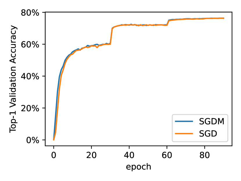
(a) SGDM and SGD with batch size 1024

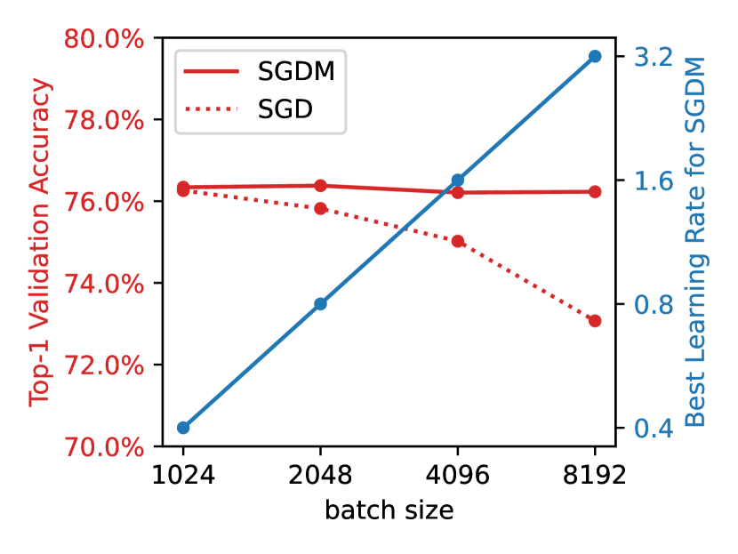
(b) SGDM v.s. SGD across batch sizes

Figure 1: SGDM performs comparably to SGD in training ResNet-50 on ImageNet with smaller batch sizes (e.g., 1024), and outperforms SGD significantly at larger batch sizes.

Language Model Experiments.

In fine-tuning a pre-trained model, a small learning rate is also preferable to retain the model’s knowledge learned during pre-training. Indeed, we observe that SGD and SGDM behave similarly in this case. We fine-tune RoBERTa-large (Liu et al., 2019) on $5$ diverse tasks (SST-2 (Socher et al., 2013), SST-5 (Socher et al., 2013), SNLI (Bowman et al., 2015), TREC (Voorhees and Tice, 2000), and MNLI (Williams et al., 2018)) using SGD and SGDM. We follow the few shot setting described in (Gao et al., 2021; Malladi et al., 2023), using a grid for SGD based on (Malladi et al., 2023) and sampling $512$ examples per class (Table 1).

Task	SST-2	SST-5	SNLI	TREC	MNLI
Zero-shot	79.0	35.5	50.2	51.4	48.8
SGD	93.4 (0.2)	55.2 (1.4)	87.1 (0.7)	96.8 (0.1)	82.3 (1.1)
SGDM	93.3 (0.4)	55.5 (1.7)	87.3 (0.6)	96.9 (0.6)	82.7 (0.8)

Table 1: SGD and SGDM for fine-tuning RoBERTa-large on $5$ tasks using $512$ examples from each class (Gao et al., 2021; Malladi et al., 2023). Results are averaged over $5$ seeds. These findings confirm that SGD and SGDM approximate each other in noisy settings.

6.2 Investigating the benefit of momentum in large-batch training

The ImageNet experiments demonstrate that momentum indeed offers benefits in large-batch training when the optimal learning rate is relatively large. We now use large-batch training experiments on CIFAR-10 to provide empirical evidence that this benefit may not be due to the noise reduction effect. We apply SVAG (Li et al., 2021a) to control the noise scale in our experiments and reduce the curvature-induced training instability (Lemma 3.4) while leaving the noise-induced term unchanged.

Definition 6.1 (SVAG).

With any $\ell>0$, SVAG transforms the NGOS $\mathcal{G}_{\sigma}=(f,{\bm{\Sigma}},\mathcal{Z}_{\sigma})$ (Definition 3.1) into another NGOS $\widehat{\mathcal{G}}_{\sqrt{\ell}\sigma}=(f,{\bm{\Sigma}},\widehat{\mathcal{Z}}_{\sqrt{\ell}\sigma})$ with scale $\sqrt{\ell}\sigma$. For an input ${\bm{\theta}}$, $\widehat{\mathcal{G}}_{\ell\sigma}$ returns $\widehat{\bm{g}}=r_{1}(\ell){\bm{g}}_{1}+r_{2}(\ell){\bm{g}}_{2}$ where ${\bm{g}}_{1},{\bm{g}}_{2}\sim\mathcal{G}_{\sigma}({\bm{\theta}})$ and $r_{i}(\ell)=\frac{1}{2}(1+(-1)^{i}\sqrt{2\ell-1})$. $\widehat{\mathcal{Z}}_{\sqrt{\ell}\sigma}$ is defined to ensure $\widehat{\bm{g}}$ has the same distribution as $\nabla f({\bm{\theta}})+\sqrt{\ell}\sigma{\bm{z}}$ when ${\bm{z}}\sim\widehat{\mathcal{Z}}_{\sqrt{\ell}\sigma}({\bm{\theta}})$.

In our experiments, we divide the learning rate $\eta$ by $\ell$ after applying SVAG so $\lambda^{\prime}=\lambda/\sqrt{\ell}$, and run $\ell$ times the original iterate steps. This ensures that way the noise-induced impact and the descent force stay the same scale in Lemma 3.4, while the curvature-induced impact is reduced by a factor of $\ell$.

We train a ResNet-32 (He et al., 2016) on CIFAR-10 (Krizhevsky et al., ) with batch size $B=512$. In order to control the curvature-induced impact, we apply SVAG (Li et al., 2021a; Malladi et al., 2022) to the NGOS (Definition 3.1) for SGD and SGDM. We first grid search to find the best learning rate for the standard SGDM ($\ell=1$), and then we perform SGD and SGDM with that same learning rate for different levels of $\ell$. The results are summarized in Figure 2. We see that standard SGDM outperforms standard SGD, but when we increase the noise level $\ell$, the two trajectories become closer.

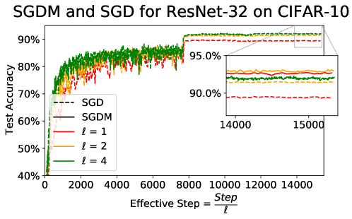
Figure 2: Standard SGDM achieves higher test performance than SGD (see $\ell=1$), but the two trajectories get closer when reducing the curvature-induced term with SVAG (i.e., increasing the value of $\ell$, see Definition 6.1 and Lemma 3.4). These experiments confirm our theoretical findings that SGD and SGDM approximate each other when the gradient noise is the primary source of instability. We use batch size $B=512$ with two learning rate decays by a factor of $0.1$ at epochs $80$ and $120$. We grid search to find the best learning rate for SGDM ($\eta=0.2$) and then use it to run SGD and SGDM with SVAG. We use $\beta=0.9$ for SGDM. Additional experimental details are in the appendix.

7 Conclusions

This work provides theoretical characterizations of the role of momentum in stochastic gradient methods. We formally show that momentum does not introduce optimization and generalization benefits when the learning rates are small, and we further exhibit empirically that the value of momentum is marginal for gradient-noise-dominated learning settings with practical learning rate scales. Hence we conclude that momentum does not provide a significant performance boost in the above cases. Our results further suggest that model performance is agnostic to the choice of momentum parameters over a range of hyperparameter scales.

Appendix A Additional Preliminaries

A.1 SGDM Formulations

Recall Definition 3.3 where we defined SGDM as following:

$${\bm{m}}_{k+1}=\beta_{k}{\bm{m}}_{k}+(1-\beta_{k}){\bm{g}}_{k},\qquad{\bm{x}}_{k+1}={\bm{x}}_{k}-\eta_{k}{\bm{m}}_{k+1}.$$ (5)

Our formulation is different from various SGDM implementations which admit the following form:

Definition A.1 (Standard formulation of SGD with momentum).

Given a stochastic gradient $\bar{{\bm{g}}}_{k}\sim\mathcal{G}_{\sigma}(\bar{{\bm{x}}}_{k})$, SGD-Standard with the hyperparameter schedule $(\gamma_{k},\mu_{k},\tau_{k})$ momentum updates the parameters $\bar{{\bm{x}}}_{k}\in\mathbb{R}^{d}$ from $(\bar{{\bm{m}}}_{0},\bar{{\bm{x}}}_{0})$ as

$$\bar{{\bm{m}}}_{k+1} =\mu_{k}\bar{{\bm{m}}}_{k}+(1-\tau_{k})\bar{{\bm{g}}}_{k}$$ (6)

$$\bar{{\bm{x}}}_{k+1} =\bar{{\bm{x}}}_{k}-\gamma_{k}\bar{{\bm{m}}}_{k+1}$$ (7)

where $\tau_{k}\in[0,1)$.

Notice that with $\tau_{k}=0$, $\mu_{k}=\beta$ and $\gamma_{k}=\gamma$, the standard formulation recovers Equation 1 that has commonly appeared in the literature. The standard formulation also recovers Equation 5 with $\mu_{k}=\tau_{k}=\beta_{k}$ and $\eta_{k}=\gamma_{k}$. Actually, as we will show in the following lemma, these formulations are equivalent up to hyperparameter transformations.

Lemma A.2 (Equivalence of SGDM and SGD-Standard).

Let $\alpha_{k}$ be the sequence that $\alpha_{0}=1$ and

$$\alpha_{k+1}=\frac{\alpha_{k}}{\alpha_{k}(1-\tau_{k})+\mu_{k}}.$$

Then $0<\alpha_{k+1}\leq\frac{1}{1-\tau_{k}}$. For parameters schedules and initialization

$$\beta_{k}=\frac{\alpha_{k+1}}{\alpha_{k}}\mu_{k},\eta_{k}=\frac{\gamma_{k}}{\alpha_{k+1}},{\bm{m}}_{0}=\bar{{\bm{m}}}_{0},{\bm{x}}_{0}=\bar{{\bm{x}}}_{0}$$

then $\bar{{\bm{x}}}_{k}$ and ${\bm{x}}_{k}$ follow the same distribution. ${\bm{x}}_{k}$ is by Definition 3.3 and $\bar{{\bm{x}}}_{k}$ by Definition A.1.

Proof.

We shall prove that given ${\bm{x}}_{k}=\bar{{\bm{x}}_{k}}$, ${\bm{g}}_{k}=\bar{{\bm{g}}}_{k}$ and ${\bm{m}}_{k}=\alpha_{k}\bar{{\bm{m}}}_{k}$, there is and ${\bm{m}}_{k+1}=\alpha_{k+1}\bar{{\bm{m}}}_{k+1}$ and $\bar{{\bm{x}}}_{k+1}={\bm{x}}_{k+1}$. This directly follows that $\alpha_{k+1}(1-\tau_{k})=1-\beta_{k}$, and

$$\bar{{\bm{m}}}_{k+1} =\mu_{k}\bar{{\bm{m}}}_{k}+(1-\tau_{k})\bar{{\bm{g}}}_{k}$$

$$=\frac{\mu_{k}}{\alpha_{k}}{\bm{m}}_{k}+(1-\tau_{k}){\bm{g}}_{k}$$

$$=\frac{1}{\alpha_{k+1}}(\beta_{k}{\bm{m}}_{k}+\alpha_{k+1}(1-\tau_{k}){\bm{g}}_{k})$$

$$=\frac{1}{\alpha_{k+1}}{\bm{m}}_{k+1}.$$

$$\bar{{\bm{x}}}_{k+1} =\bar{{\bm{x}}}_{k}-\gamma_{k}\bar{{\bm{m}}}_{k+1}$$

$$={\bm{x}}_{k}-\eta_{k}{\bm{m}}_{k+1}.$$

Then we can prove the claim by induction that ${\bm{x}}_{k}$ and $\bar{{\bm{x}}_{k}}$ are identical in distribution. More specifically, we shall prove that the CDF for $({\bm{x}}_{k},{\bm{m}}_{k},{\bm{g}}_{k})$ at $({\bm{x}},{\bm{m}},{\bm{g}})$ is the same as the CDF for $(\bar{{\bm{x}}}_{k},\bar{{\bm{m}}}_{k},\bar{{\bm{g}}}_{k})$ at $({\bm{x}},\frac{{\bm{m}}}{\alpha_{k}},{\bm{g}})$. For $k=0$, the claim is trivial. If the induction premise holds for $k$, then let $({\bm{x}}_{k+1},{\bm{m}}_{k+1},{\bm{g}}_{k+1})$ be the one-step iterate in Equation 5 from $({\bm{x}}_{k},{\bm{m}}_{k},{\bm{g}}_{k})=({\bm{x}},{\bm{m}},{\bm{g}})$ and $(\bar{{\bm{x}}}_{k+1},\bar{{\bm{m}}}_{k+1},\bar{{\bm{g}}}_{k+1})$ be the one-step iterate in Definition A.1 from $(\bar{{\bm{x}}}_{k},\bar{{\bm{m}}}_{k},\bar{{\bm{g}}}_{k})=({\bm{x}},\frac{{\bm{m}}}{\alpha_{k}},{\bm{g}})$, then we know from above that $\alpha_{k+1}\bar{{\bm{m}}}_{k+1}={\bm{m}}_{k+1}$ and $\bar{{\bm{x}}}_{k+1}={\bm{x}}_{k+1}$, and therefore the conditional distribution for $({\bm{x}}_{k+1},{\bm{m}}_{k+1},{\bm{g}}_{k+1})$ is the same as that for $(\bar{{\bm{x}}}_{k+1},\alpha_{k+1}\bar{{\bm{m}}}_{k+1},\bar{{\bm{g}}}_{k+1})$. Integration proves the claim for $k+1$, and thereby the induction is complete. ∎

Therefore, in the rest part of the appendix, we will stick to the formulation of SGDM as Equation 5 unless specified otherwise.

A.2 Descent Lemma for Momentum

Assume $\|{\bm{m}}\|=\mathcal{O}(1)$ and $1-\beta\ll\eta$. For the SGDM update ${\bm{x}}_{k}$, the expected change in loss per step is

$$\mathbb{E}\mathcal{L}({\bm{x}}_{k+1}) =\mathbb{E}\mathcal{L}({\bm{x}}_{k})-\eta\mathbb{E}\left\|\nabla\mathcal{L}({\bm{x}}_{k})\right\|^{2}$$

$$+\frac{1}{2}\eta^{2}\mathbb{E}(\nabla\mathcal{L}^{\top}(\nabla^{2}\mathcal{L})\nabla\mathcal{L}({\bm{x}}_{k})+\mathop{\mathrm{tr}}((\nabla^{2}\mathcal{L})\sigma\sigma^{\top}({\bm{x}}_{k})))+o(\eta^{2})$$

$$+\frac{\eta\beta}{1-\beta}(S_{k+1}-S_{k})+\eta^{2}\mathbb{E}[{\bm{m}}_{k}^{\top}\nabla^{2}\mathcal{L}\nabla\mathcal{L}({\bm{x}}_{k})].$$

where $S_{k}=\mathbb{E}[\nabla\mathcal{L}({\bm{x}}_{k})^{\top}{\bm{m}}_{k}-\frac{\eta}{2}{\bm{m}}_{k}^{\top}\nabla^{2}\mathcal{L}({\bm{x}}_{k}){\bm{m}}_{k}]$. )

Appendix B The dynamics of SGDM in $O(1/\eta)$ time

In this section we will prove Theorem 4.5 as the first part of our main result. First we shall take a closer examination at our update rule in Definition 3.3. Let $\beta_{s:t}=\prod_{r=s}^{t}\beta_{r}$ be the product of consecutive momentum hyperparameters for $s\leq t$, and define $\beta_{s:t}=1$ for $s>t$, we get the following expansion forms.

Lemma B.1.

$${\bm{m}}_{k} =\beta_{0:k-1}{\bm{m}}_{0}+\sum_{s=0}^{k-1}\beta_{s+1:k-1}(1-\beta_{s}){\bm{g}}_{s}$$

$${\bm{x}}_{k} ={\bm{x}}_{0}-\sum_{s=0}^{k-1}\eta_{s}\beta_{0:s}{\bm{m}}_{0}-\sum_{s=0}^{k-1}\sum_{r=s}^{k-1}\eta_{r}\beta_{s+1:r}(1-\beta_{s}){\bm{g}}_{s}$$

Proof.

By expansion of Equation 3. ∎

Let the coefficients $c_{s,k}=\sum_{r=s}^{k-1}\eta_{r}\beta_{s+1:r}(1-\beta_{s})$ so that ${\bm{x}}_{k}={\bm{x}}_{0}-\frac{\beta_{0}c_{0:k}}{1-\beta_{0}}{\bm{m}}_{0}-\sum_{s=0}^{k-1}c_{s,k}{\bm{g}}_{s}$. Notice that $c_{s,k}$ is increasing in $k$ but it is always upper-bounded as $c_{s,k}\leq c_{s,\infty}=\sum_{r=s}^{\infty}\eta_{r}\beta_{s+1:r}(1-\beta_{s})\leq(\sup_{t}\eta_{t})\sum_{r=s}^{\infty}(\sup_{t}\beta_{t})^{r-s}=\frac{\sup_{r}\eta_{r}}{1-\sup_{t}\beta_{t}}$. Furthermore, if for any $t$, $\beta_{t}$ and $\eta_{t}$ are about the same scale, then we should expect that the difference $c_{s,\infty}-c_{s,k}$ is exponentially small in $k$. Then we can hypothesize that the trajectory ${\bm{x}}_{k}$ should be close to a trajectory of the following form:

$$\widetilde{{\bm{x}}}_{k}=\widetilde{{\bm{x}}}_{0}-\frac{\beta_{0}c_{0:\infty}}{1-\beta_{0}}{\bm{m}}_{0}-\sum_{s=0}^{k-1}c_{s,\infty}\widetilde{{\bm{g}}}_{s}$$

which is exactly a SGD trajectory given the learning rate schedule $c_{s,\infty}$.

To formalize the above thought, we define the averaged learning rate schedule

$$\bar{\eta}_{k}=c_{k,\infty}=\sum_{s=k}^{\infty}\eta_{s}\beta_{k+1:s}(1-\beta_{k})$$ (8)

And the coupled trajectory

$${\bm{y}}_{k} ={\bm{x}}_{k}-\frac{\bar{\eta}_{k}\beta_{k}}{1-\beta_{k}}{\bm{m}}_{k}$$ (9)

$$={\bm{x}}_{0}-\frac{\beta_{0}\bar{\eta}_{0}}{1-\beta_{0}}{\bm{m}}_{0}-\sum_{s=0}^{k-1}\bar{\eta}_{s}{\bm{g}}_{s}.$$ (10)

Then there is the following transition:

$${\bm{y}}_{k}={\bm{y}}_{k-1}-\bar{\eta}_{k-1}{\bm{g}}_{k-1}$$ (11)

${\bm{y}}_{k}$ has an interesting geometrical interpretation as the endpoint of SGDM if we cut-off all the gradient signal from step $k$. E.g., ${\bm{x}}_{\infty}$ if we set ${\bm{g}}_{k+1}={\bm{g}}_{k+2}=\cdots=0$ for and update the SGDM from (${\bm{x}}_{k}$,${\bm{m}}_{k}$).

B.1 $\alpha\in[0,1)$

In this section we provide the proof for Theorem 4.5. Specifically, when $\alpha\in[0,1)$ is the index for the control of the learning rate schedule (Definition 4.1), we hope to show that ${\bm{y}}_{k}$ is close to a SGD trajectory ${\bm{z}}_{k}$, defined by the following for $k\geq 0$:

$${\bm{z}}_{0}={\bm{x}}_{0}$$ (12)

$${\bm{h}}_{k}\sim\mathcal{G}_{\sigma}({\bm{z}}_{k})$$ (13)

$${\bm{z}}_{k+1}={\bm{z}}_{k}-\bar{\eta}_{k}{\bm{h}}_{k}$$ (14)

Specifically, we use ${\bm{y}}_{k}$ as a bridge for connecting ${\bm{x}}_{k}$ and ${\bm{z}}_{k}$. Our proof consists of two steps.

1. We show that ${\bm{x}}_{k}$ and ${\bm{y}}_{k}$ are order-$(1-\alpha)/2$ weak approximations of each other.

2. We show that ${\bm{z}}_{k}$ and ${\bm{y}}_{k}$ are order-$(1-\alpha)/2$ weak approximations of each other.

Then we can conclude that ${\bm{x}}_{k}$ and ${\bm{z}}_{k}$ are order-$(1-\alpha)/2$ weak approximations of each other, which states our main theorem Theorem 4.5.

First, we give a control of the averaged learning rate $\bar{\eta}_{k}$ (Equation 8) with the following lemma.

Lemma B.2.

Let $(\eta_{k},\beta_{k})$ be a learning rate schedule scaled by $\eta$ (Definition 4.1) with index $\alpha$, and $\bar{\eta}_{k}$ be the averaged learning rate (Equation 8), there is

$$\bar{\eta}_{k}\leq\frac{\lambda_{\max}\eta_{\max}}{\lambda_{\min}}\eta$$

$$\frac{\bar{\eta}_{k}\beta_{k}}{1-\beta_{k}}\leq\frac{\lambda_{\max}\eta_{\max}}{\lambda^{2}_{\min}}\eta^{1-\alpha}.$$

Proof.

By Definition 4.1 we know $\beta_{k}\in[1-\lambda_{\max}\eta^{\alpha},1-\lambda_{\min}\eta^{\alpha}]$ and $\eta_{k}\leq\eta_{\max}\eta$. Therefore

$$\bar{\eta}_{k} =\sum_{s=k}^{\infty}\eta_{s}\beta_{k+1:s}(1-\beta_{k})$$

$$\leq\sum_{s=k}^{\infty}\eta_{\max}\eta(1-\lambda_{\min}\eta^{\alpha})^{s-k}\lambda_{\max}\eta^{\alpha}$$

$$=\frac{\lambda_{\max}\eta_{\max}}{\lambda_{\min}}\eta.$$

$$\frac{\bar{\eta}_{k}\beta_{k}}{1-\beta_{k}} \leq\frac{\lambda_{\max}\eta_{\max}}{\lambda_{\min}}\eta\cdot\frac{1}{1-\beta_{k}}$$

$$\leq\frac{\lambda_{\max}\eta_{\max}}{\lambda^{2}_{\min}}\eta^{1-\alpha}.$$

∎

B.1.1 Step 1

For the first step we are going to proof the following Theorem B.3. For notation simplicity we omit the superscript $\eta$ for the scaling when there is no ambiguity.

Theorem B.3 (Weak Approximation of Coupled Trajectory).

With the learning rate schedule $(\eta_{k},\beta_{k})$ scaled by $\eta$ with index $\alpha\in[0,1)$. Assume that the NGOS $\mathcal{G}_{\sigma}$ satisfy Assumption 4.3 and the initialization ${\bm{m}}_{0}$ satisfy Assumption 4.2. For any noise scale $\sigma\leq\eta^{-1/2}$, let $({\bm{x}}_{k},{\bm{m}}_{k})$ be the SGDM trajectory and ${\bm{y}}_{k}$ be the corresponding coupled trajectory (Equation 9). Then, the coupled trajectory ${\bm{y}}_{k}$ is an order-$\gamma$ weak approximation (Definition 4.4) to ${\bm{x}}_{k}$ with $\gamma=(1-\alpha)/2$.

For notations, let $\nabla_{k}=\nabla\mathcal{L}({\bm{x}}_{k})$ so ${\bm{g}}_{k}=\nabla_{k}+\sigma{\bm{v}}_{k}$ is the stochastic gradient sampled from the NGOS. Also by Assumption 4.3, as ${\bm{\Sigma}}^{1/2}$ is bounded, let $C_{\mathop{\mathrm{tr}}}>0$ be the constant that $\mathop{\mathrm{tr}}{\bm{\Sigma}}({\bm{x}})\leq C_{\mathop{\mathrm{tr}}}$ for all ${\bm{x}}\in{\mathbb{R}}^{d}$. As $\nabla\mathcal{L}$ is Lipschitz, let $L>0$ be the constant that $\left\|\nabla\mathcal{L}({\bm{x}})-\nabla\mathcal{L}({\bm{y}})\right\|\leq L\left\|{\bm{x}}-{\bm{y}}\right\|$ for all ${\bm{x}},{\bm{y}}\in{\mathbb{R}}^{d}$. As ${\bm{\Sigma}}^{1/2}$ is Lipschitz and bounded, let $L_{\Sigma}>0$ be the constant that $|\mathop{\mathrm{tr}}{{\bm{\Sigma}}({\bm{x}})-{\bm{\Sigma}}({\bm{y}})}|\leq L_{\Sigma}\left\|{\bm{x}}-{\bm{y}}\right\|$ for all ${\bm{x}},{\bm{y}}\in{\mathbb{R}}^{d}$

To show the result it suffices to bound $\mathbb{E}\left\|{\bm{x}}_{k}\right\|^{2m}$ and $\mathbb{E}\left\|{\bm{m}}_{k}\right\|$ for any $m\geq 0$ and $k=O(\eta^{-1})$. As the gradient noises are scaled with variance $O(\sigma^{2})=O(\eta^{-1})$ so that may dominate the expansion Lemma B.1. We will show that $\mathbb{E}\left\|{\bm{m}}_{k}\right\|=O(\eta^{(\alpha-1)/2})$ is the correct scale so we still have $\mathbb{E}\left\|{\bm{x}}_{k}\right\|^{2m}=O(1)$. An useful inequality we will use often in our proof is the Grönwall’s inequality

Lemma B.4 (Grönwall’s Inequality).

For non-negative sequences $\{f_{i},g_{i},k_{i}\in{\mathbb{R}}\}_{i\geq 0}$, if for all $t>0$

$$f_{t}\leq g_{t}+\sum_{s=0}^{t-1}k_{s}f_{s}$$

then $f_{t}\leq g_{t}+\sum_{s=0}^{t-1}k_{s}g_{s}\exp(\sum_{r=s+1}^{t-1}k_{r})$.

Next follows the proofs.

Lemma B.5.

We can bound the expected norm of

$$\mathbb{E}\left\|{\bm{m}}_{k}\right\|^{2}\leq 12\frac{\lambda^{2}_{\max}}{\lambda^{2}_{\min}}\sup_{\tau=1,...,k}\mathbb{E}(\|\nabla_{\tau}\|)^{2}+(4+8\frac{L\eta_{\max}}{\lambda_{\min}}+\eta^{\alpha-1})K_{0}$$ (15)

with constant $K_{0}=\frac{2\lambda^{2}_{\max}}{\lambda_{\min}}C_{\mathop{\mathrm{tr}}}+3\mathbb{E}\left\|{\bm{m}}_{0}\right\|^{2}=\frac{2\lambda^{2}_{\max}}{\lambda_{\min}}C_{\mathop{\mathrm{tr}}}+3C_{2}$ ($C_{2}$ by Assumption 4.2), for a small enough learning rate $\eta<\left(\frac{\lambda_{\min}}{4L\eta_{\max}}\right)^{\frac{1}{1-\alpha}}$.

Proof.

To bound $\mathbb{E}\left\|{\bm{m}}_{k}\right\|^{2}$, we unroll the momentum by Lemma B.1 and write

$${\bm{m}}_{k} =\beta_{0:k-1}{\bm{m}}_{0}+\sum_{s=0}^{k-1}\beta_{s+1:k-1}(1-\beta_{s}){\bm{g}}_{s}$$ (16)

Define

$$\widetilde{{\bm{m}}}_{k} =\beta_{0:k-1}{\bm{m}}_{0}+\sum_{s=0}^{k-1}\beta_{s+1:k-1}(1-\beta_{s})\nabla_{s}.$$

Then $\mathbb{E}{\bm{m}}_{k}=\mathbb{E}\widetilde{{\bm{m}}}_{k}$, and

$${\bm{m}}_{k}-\widetilde{{\bm{m}}}_{k} =\sum_{s=0}^{k-1}\beta_{s+1:k-1}(1-\beta_{s})\sigma{\bm{v}}_{s}$$

Let constant $K_{0}=2C_{\mathop{\mathrm{tr}}}+3C_{2}$, we can write

$$\mathbb{E}\left\|{\bm{m}}_{k}\right\|^{2} \leq\mathbb{E}(\left\|\widetilde{{\bm{m}}}_{k}\right\|+\left\|{\bm{m}}_{k}-\widetilde{{\bm{m}}}_{k}\right\|)^{2}$$ (17)

$$\leq 2\mathbb{E}\left\|\widetilde{{\bm{m}}}_{k}\right\|^{2}+2\mathbb{E}\left\|{\bm{m}}_{k}-\widetilde{{\bm{m}}}_{k}\right\|^{2}$$ (18)

$$=2\mathbb{E}\left\|\widetilde{{\bm{m}}}_{k}\right\|^{2}+2\sum_{s=0}^{k-1}(\beta_{s+1:k-1})^{2}(1-\beta_{s})^{2}\sigma^{2}\mathbb{E}\mathop{\mathrm{tr}}{\bm{\Sigma}}({\bm{x}}_{s})$$ (19)

$$\leq 2\mathbb{E}\left\|\widetilde{{\bm{m}}}_{k}\right\|^{2}+2\sum_{s=0}^{k-1}(1-\lambda_{\min}\eta^{\alpha})^{2(k-s-1)}\lambda^{2}_{\max}\eta^{2\alpha}\sigma^{2}\mathbb{E}\mathop{\mathrm{tr}}{\bm{\Sigma}}({\bm{x}}_{s})$$ (20)

$$\leq 2\mathbb{E}\left\|\widetilde{{\bm{m}}}_{k}\right\|^{2}+\eta^{\alpha-1}\frac{2\lambda^{2}_{\max}}{\lambda_{\min}}C_{\mathop{\mathrm{tr}}}$$ (21)

$$\leq 2\mathbb{E}\left\|\widetilde{{\bm{m}}}_{k}\right\|^{2}+\eta^{\alpha-1}K_{0}.$$ (22)

On the other hand, we know

$$\widetilde{{\bm{m}}}_{k} =\beta_{0:k-1}{\bm{m}}_{0}+\sum_{s=0}^{k-1}\beta_{s+1:k-1}(1-\beta_{s})\nabla_{s}$$

We use the Lipschitzness of $\nabla$ to write

$$\|\nabla_{s}-\nabla_{k}\| \leq L\|{\bm{x}}_{s}-{\bm{x}}_{k}\|\leq L\sum_{\tau=s}^{k-1}\eta_{\tau}\left\|{\bm{m}}_{\tau+1}\right\|,$$

then we can write

$$\mathbb{E}\left\|\widetilde{{\bm{m}}}_{k}\right\|^{2} \leq\mathbb{E}\left(\beta_{0:k-1}\left\|{\bm{m}}_{0}\right\|+\sum_{s=0}^{k-1}\beta_{s+1:k-1}(1-\beta_{s})(\|\nabla_{k}\|+L\sum_{\tau=s}^{k-1}\eta_{\tau}\left\|{\bm{m}}_{\tau+1}\right\|)\right)^{2}$$

$$\leq\mathbb{E}\left(\left\|{\bm{m}}_{0}\right\|+\frac{\lambda_{\max}}{\lambda_{\min}}\|\nabla_{k}\|+L\eta\eta_{\max}\sum_{\tau=0}^{k-1}(1-\lambda_{\min}\eta^{\alpha})^{k-1-\tau}\|{\bm{m}}_{\tau+1}\|\right)^{2}$$

$$\leq 3\mathbb{E}(\left\|{\bm{m}}_{0}\right\|)^{2}+3\frac{\lambda^{2}_{\max}}{\lambda^{2}_{\min}}\mathbb{E}(\|\nabla_{k}\|)^{2}+3L^{2}\eta^{2}\eta_{\max}^{2}\left(\sum_{\tau=0}^{k-1}(1-\lambda_{\min}\eta^{\alpha})^{k-1-\tau}\right)\cdot$$

$$\qquad\left(\sum_{\tau=0}^{k-1}(1-\lambda_{\min}\eta^{\alpha})^{k-1-\tau}\mathbb{E}\|{\bm{m}}_{\tau+1}\|^{2}\right)$$

$$\leq K_{0}+3\frac{\lambda^{2}_{\max}}{\lambda^{2}_{\min}}\mathbb{E}(\|\nabla_{k}\|)^{2}+\frac{3L^{2}\eta_{\max}^{2}\eta^{2-2\alpha}}{\lambda_{\min}^{2}}\sup_{\tau=1\cdots{k}}\mathbb{E}\|{\bm{m}}_{\tau}\|^{2}.$$

Then by Equation 22, we know

$$\sup_{\tau=1,...,k}\mathbb{E}\|{\bm{m}}_{\tau}\|^{2}\leq 2\sup_{\tau=1,...,k}\mathbb{E}\left\|\widetilde{{\bm{m}}}_{\tau}\right\|^{2}+\eta^{\alpha-1}K_{0},$$

so

$$\sup_{\tau=1,...,k}\mathbb{E}\left\|\widetilde{{\bm{m}}}_{\tau}\right\|^{2} \leq K_{0}+3\frac{\lambda^{2}_{\max}}{\lambda^{2}_{\min}}\sup_{\tau=1,...,k}\mathbb{E}(\|\nabla_{\tau}\|)^{2}+\frac{6L^{2}\eta_{\max}^{2}\eta^{1-\alpha}}{\lambda_{\min}^{2}}K_{0}$$ (23)

$$\qquad+\frac{6L^{2}\eta_{\max}^{2}\eta^{2-2\alpha}}{\lambda_{\min}^{2}}\sup_{\tau=1,\cdots,{k}}\mathbb{E}\|\widetilde{{\bm{m}}}_{\tau}\|^{2}$$ (24)

Choose $\eta$ small enough so that $\frac{6L^{2}\eta_{\max}^{2}\eta^{2-2\alpha}}{\lambda_{\min}^{2}}<\frac{1}{2}$, we know

$$\sup_{\tau=1,...,k}\mathbb{E}\left\|\widetilde{{\bm{m}}}_{\tau}\right\|^{2} \leq 6\frac{\lambda^{2}_{\max}}{\lambda^{2}_{\min}}\sup_{\tau=1,...,k}\mathbb{E}(\|\nabla_{\tau}\|)^{2}+(2+2\frac{\sqrt{3}L\eta_{\max}}{\lambda_{\min}})K_{0}.$$ (25)

So

$$\mathbb{E}\left\|{\bm{m}}_{k}\right\|^{2} \leq 2\mathbb{E}\left\|\widetilde{{\bm{m}}}_{k}\right\|^{2}+\eta^{\alpha-1}K_{0}$$ (26)

$$\leq 12\frac{\lambda^{2}_{\max}}{\lambda^{2}_{\min}}\sup_{\tau=1,...,k}\mathbb{E}(\|\nabla_{\tau}\|)^{2}+(4+8\frac{L\eta_{\max}}{\lambda_{\min}}+\eta^{\alpha-1})K_{0}.$$ (27)

∎

Lemma B.6.

There is a function $f$, irrelevant to $\eta$, of polynomial growth in ${\bm{m}}_{0}$ and ${\bm{x}}_{0}$, such that

$$\sup_{k=0,...,\lfloor T/\eta\rfloor}\mathbb{E}\left\|\nabla_{k}\right\|^{2}\leq f({\bm{m}}_{0},{\bm{x}}_{0},T)$$

when $\eta<\min(\left(\frac{\lambda_{\min}^{3}}{12L\lambda_{\max}^{2}\eta_{\max}}\right)^{\frac{1}{1-\alpha}},1)$

Proof.

By the Lipschitzness of $\nabla\mathcal{L}$, we know

$$\|\nabla_{k}\| \leq\|\nabla_{0}\|+L\left\|{\bm{x}}_{k}-{\bm{x}}_{0}\right\|$$ (28)

$$\leq\|\nabla_{0}\|+L\left\|{\bm{y}}_{k}-{\bm{y}}_{0}\right\|+L\left\|{\bm{x}}_{0}-{\bm{y}}_{0}\right\|+L\left\|{\bm{x}}_{k}-{\bm{y}}_{k}\right\|$$ (29)

Observe that $\|{\bm{x}}_{k}-{\bm{y}}_{k}\|=\frac{\bar{\eta}_{k}\beta_{k}}{1-\beta_{k}}\|{\bm{m}}_{k}\|\leq\frac{\lambda_{\max}\eta_{\max}}{\lambda_{\min}^{2}}\eta^{1-\alpha}\|{\bm{m}}_{k}\|$. Let $d_{k}=\mathbb{E}\|{\bm{y}}_{k}-{\bm{y}}_{0}\|^{2}$. As a result, we can write

$$\mathbb{E}\|\nabla_{k}\|^{2} \leq 3\mathbb{E}\left(\|\nabla_{0}\|+\frac{L\lambda_{\max}\eta_{\max}}{\lambda_{\min}^{2}}\eta^{1-\alpha}\|{\bm{m}}_{0}\|\right)^{2}+3\left(\frac{L\lambda_{\max}\eta_{\max}}{\lambda_{\min}^{2}}\eta^{1-\alpha}\right)^{2}\mathbb{E}(\|{\bm{m}}_{k}\|^{2})+3L^{2}d_{k}.$$ (30)

Choose $\eta$ such that $\eta^{1-\alpha}<\frac{\lambda_{\min}^{3}}{12L\lambda_{\max}^{2}\eta_{\max}}$ and let the function

$$K_{1}({\bm{m}}_{0},{\bm{x}}_{0}) =3\mathbb{E}\left(\|\nabla\mathcal{L}({\bm{x}}_{0})\|+\frac{\lambda_{\min}}{12\lambda_{\max}}\|{\bm{m}}_{0}\|\right)^{2}$$ (31)

$$\qquad+\left(\frac{\lambda_{\min}}{6\lambda_{\max}}\right)^{2}(3+6\frac{L\eta_{\max}}{\lambda_{\min}})K_{0}+\left(\frac{L\eta_{\max}}{4\lambda_{\min}}\right)K_{0}$$ (32)

where recall $K_{0}$ is the constant from Lemma B.5. Plug Equation 15 into Equation 30 gives

$$\mathbb{E}\|\nabla_{k}\|^{2} \leq K_{1}+\frac{1}{2}\sup_{\tau=1,...,k}\mathbb{E}(\|\nabla_{\tau}\|)^{2}+3L^{2}d_{k}.$$ (33)

therefore

$$\mathbb{E}\|\nabla_{k}\|^{2}\leq 2K_{1}+6L^{2}\sup_{\tau=1,...,k}d_{\tau}.$$ (34)

Now we need to bound $d_{k}$ by iteration.

$$d_{k+1} =d_{k}+\mathbb{E}\|{\bm{y}}_{k+1}-{\bm{y}}_{k}\|^{2}+2\mathbb{E}({\bm{y}}_{k+1}-{\bm{y}}_{k})^{\top}({\bm{y}}_{k}-{\bm{y}}_{0})$$ (35)

$$=d_{k}+\bar{\eta}_{k}^{2}\mathbb{E}\left\|\nabla_{k}\right\|^{2}+\bar{\eta}_{k}^{2}\sigma^{2}\mathbb{E}\mathop{\mathrm{tr}}({\bm{\Sigma}}({\bm{x}}_{k}))+2\mathbb{E}(\nabla_{k})^{\top}({\bm{y}}_{k}-{\bm{y}}_{0})$$ (36)

$$\leq d_{k}+\frac{\lambda^{2}_{\max}}{\lambda^{2}_{\min}}\eta_{\max}^{2}\eta^{2}\mathbb{E}\left\|\nabla_{k}\right\|^{2}+\frac{\lambda^{2}_{\max}}{\lambda^{2}_{\min}}\eta_{\max}^{2}\eta C_{\mathop{\mathrm{tr}}}+2\frac{\lambda_{\max}}{\lambda_{\min}}\eta_{\max}\eta\sqrt{d_{k}\mathbb{E}\left\|\nabla_{k}\right\|^{2}}$$ (37)

Let function $K_{2}({\bm{m}}_{0},{\bm{x}}_{0})=\frac{\lambda^{2}_{\max}}{\lambda^{2}_{\min}}\eta_{\max}^{2}C_{\mathop{\mathrm{tr}}}+2\frac{\lambda^{2}_{\max}}{\lambda^{2}_{\min}}\eta_{\max}^{2}K_{1}({\bm{m}}_{0},{\bm{x}}_{0})+2\frac{\lambda_{\max}}{\lambda_{\min}}\eta_{\max}\frac{K_{1}({\bm{m}}_{0},{\bm{x}}_{0})}{\sqrt{6}L}$, and $\bar{d}_{k}=\sup_{\tau=1,...,k}d_{\tau}$. We know

$$\sqrt{d_{k}\mathbb{E}\left\|\nabla_{k}\right\|^{2}} \leq\sqrt{6L^{2}}d_{k}+\frac{K_{1}}{\sqrt{6L^{2}}},$$ (38)

$$\bar{d}_{k+1} \leq\bar{d}_{k}+K_{2}\eta+6L^{2}\frac{\lambda^{2}_{\max}}{\lambda^{2}_{\min}}\eta_{\max}^{2}\eta^{2}\bar{d}_{k}+2\frac{\lambda_{\max}}{\lambda_{\min}}\eta_{\max}\eta(\sqrt{6}L\bar{d}_{k})$$ (39)

$$\leq(1+6L\frac{\lambda_{\max}\eta_{\max}}{\lambda_{\min}}\eta+6L^{2}\frac{\lambda^{2}_{\max}\eta_{\max}^{2}}{\lambda^{2}_{\min}}\eta^{2})\bar{d}_{k}+\eta K_{2}$$ (40)

Let $\kappa=1+6L\frac{\lambda_{\max}\eta_{\max}}{\lambda_{\min}}\eta+6L^{2}\frac{\lambda^{2}_{\max}\eta_{\max}^{2}}{\lambda^{2}_{\min}}\eta^{2}$, then by Grönwall’s inequality Lemma C.10,

$$\bar{d}_{k} \leq\eta K_{2}(1+\sum_{s=0}^{k-1}\kappa\exp^{\kappa s})$$ (41)

$$\leq K_{2}+K_{2}T\exp^{1+6L\frac{\lambda_{\max}\eta_{\max}}{\lambda_{\min}}T+6L^{2}\frac{\lambda^{2}_{\max}\eta_{\max}^{2}}{\lambda^{2}_{\min}}T}.$$ (42)

Plugging into Equation 34 finished the proof. ∎

Lemma B.7.

There is a function $f$, irrelevant to $\eta$, of polynomial growth in ${\bm{m}}_{0}$ and ${\bm{x}}_{0}$, such that

$$\mathbb{E}\left\|{\bm{m}}_{k}\right\|^{2}\leq\eta^{\alpha-1}f({\bm{m}}_{0},{\bm{x}}_{0},T)$$

for all $k\leq\frac{T}{\eta}$.

Proof.

The result directly follows from Lemma B.5 and Lemma B.6. ∎

Lemma B.8.

There exists function $h$ that, for all $k\leq\frac{T}{\eta}$,

$$\mathbb{E}[(1+\|{\bm{x}}_{k}\|^{2})^{m}] \leq h({\bm{m}}_{0},{\bm{x}}_{0},m,T),$$

$$\mathbb{E}[(1+\|{\bm{y}}_{k}\|^{2})^{m}] \leq h({\bm{m}}_{0},{\bm{x}}_{0},m,T),$$

$$\mathbb{E}[\eta^{m}\|{\bm{g}}_{k}\|^{2m}] \leq h({\bm{m}}_{0},{\bm{x}}_{0},m,T),$$

and that $h$ is irrelevant to $k$ and $\eta$.

Proof.

We use the fact that $(a+b)^{m}\leq 2^{m-1}(a^{m}+b^{m})$ from the Jensen inequality for $a,b>0$ and $m\geq 1$. Furthermore by Young’s inequality $a^{\alpha}b^{\beta}\leq\frac{\alpha a^{\alpha+\beta}+\beta b^{\alpha+\beta}}{\alpha+\beta}\leq a^{\alpha+\beta}+b^{\alpha+\beta}$ for $\alpha,\beta>0$.

$$\left\|{\bm{g}}_{k}\right\|^{2m} \leq(\|\nabla_{k}\|+\sigma\|{\bm{v}}_{k}\|)^{2m}$$ (43)

$$\leq 2^{2m-1}(\|\nabla_{k}\|^{2m}+\eta^{-m}\|{\bm{v}}_{k}\|^{2m})$$ (44)

$$\|\nabla_{k}\|^{2m} \leq(\|\nabla_{0}\|+L\|{\bm{x}}_{k}-{\bm{x}}_{0}\|)^{2m}$$ (45)

$$\leq 2^{2m-1}((\|\nabla_{0}\|+L\|{\bm{x}}_{0}\|)^{2m}+L^{2m}\|{\bm{x}}_{k}\|^{2m})$$ (46)

The term $\mathbb{E}\left\|{\bm{v}}_{k}\right\|^{2m}$ is bounded by Assumption 4.3. Now we need to show the bounds on $\mathbb{E}[(1+\|{\bm{x}}_{k}\|^{2})^{m}]$ and $\mathbb{E}[(1+\|{\bm{y}}_{k}\|^{2})^{m}]$. Specifically we shall prove $\mathbb{E}[(1+\|{\bm{y}}_{k}\|^{2}+\eta^{2-2\alpha}\|{\bm{m}}_{k}\|^{2})^{m}]\leq h({\bm{m}}_{0},{\bm{x}}_{0},m,T)$.

Let

$$\delta_{k} =\bar{\eta}_{k}^{2}\left\|{\bm{g}}_{k}\right\|^{2}-2\bar{\eta}_{k}\langle{{\bm{g}}_{k}},{{\bm{y}}_{k}}\rangle+\eta^{2-2\alpha}(\left\|\beta_{k}{\bm{m}}_{k}+(1-\beta_{k}){\bm{g}}_{k}\right\|^{2}-\left\|{\bm{m}}_{k}\right\|^{2}),$$

then there is

$$\qquad\mathbb{E}[(1+\|{\bm{y}}_{k+1}\|^{2}+\eta^{2-2\alpha}\|{\bm{m}}_{k+1}\|^{2})^{m}|{\bm{y}}_{k},{\bm{m}}_{k}]$$

$$=\mathbb{E}[(1+\|{\bm{y}}_{k}-\bar{\eta}_{k}{\bm{g}}_{k}\|^{2}+\eta^{2-2\alpha}\left\|\beta_{k}{\bm{m}}_{k}+(1-\beta_{k}){\bm{g}}_{k}\right\|^{2})^{m}|{\bm{y}}_{k},{\bm{m}}_{k}]$$

$$=\mathbb{E}[(1+\|{\bm{y}}_{k}\|^{2}+\eta^{2-2\alpha}\|{\bm{m}}_{k}\|^{2}+\delta_{k})^{m}|{\bm{y}}_{k},{\bm{m}}_{k}]$$

$$\leq(1+\left\|{\bm{y}}_{k}\right\|^{2}+\eta^{2-2\alpha}\|{\bm{m}}_{k}\|^{2})^{m}+m(1+\left\|{\bm{y}}_{k}\right\|^{2}+\eta^{2-2\alpha}\|{\bm{m}}_{k}\|^{2})^{m-1}\mathbb{E}[\delta_{k}|{\bm{y}}_{k},{\bm{m}}_{k}]$$

$$+\mathbb{E}[\delta_{k}^{2}\sum_{i=0}^{m-2}\binom{m}{i+2}\delta_{k}^{i}(1+\left\|{\bm{y}}_{k}\right\|^{2}+\eta^{2-2\alpha}\|{\bm{m}}_{k}\|^{2})^{m-2-i}|{\bm{y}}_{k},{\bm{m}}_{k}]$$

$$\leq(1+\left\|{\bm{y}}_{k}\right\|^{2}+\eta^{2-2\alpha}\|{\bm{m}}_{k}\|^{2})^{m}+m(1+\left\|{\bm{y}}_{k}\right\|^{2}+\eta^{2-2\alpha}\|{\bm{m}}_{k}\|^{2})^{m-1}\mathbb{E}[\delta_{k}|{\bm{y}}_{k},{\bm{m}}_{k}]$$

$$+2^{m}\mathbb{E}[\delta_{k}^{2}(|\delta_{k}|^{m-2}+(1+\left\|{\bm{y}}_{k}\right\|^{2}+\eta^{2-2\alpha}\|{\bm{m}}_{k}\|^{2})^{m-2})|{\bm{y}}_{k},{\bm{m}}_{k}].$$

Then there exists constant $K_{3}$ such that

$$\mathbb{E}[\delta_{k}|{\bm{y}}_{k},{\bm{m}}_{k}] =\bar{\eta}_{k}^{2}\left\|\nabla_{k}\right\|^{2}+\bar{\eta}_{k}^{2}\sigma^{2}\mathbb{E}\mathop{\mathrm{tr}}{\bm{\Sigma}}({\bm{x}}_{k})-2\bar{\eta}_{k}\langle{\nabla_{k}},{{\bm{y}}_{k}}\rangle+\eta^{2-2\alpha}(\left\|\beta_{k}{\bm{m}}_{k}+(1-\beta_{k}){\bm{g}}_{k}\right\|^{2}-\left\|{\bm{m}}_{k}\right\|^{2})$$

$$\leq\mathbb{E}_{|{\bm{y}}_{k}}\frac{\lambda^{2}_{\max}\eta^{2}_{\max}}{\lambda^{2}_{\min}}(2\eta^{2}(\|\nabla_{0}\|+L\|{\bm{x}}_{0}\|)^{2}+2\eta^{2}L^{2}\|{\bm{x}}_{k}\|^{2}+\eta C_{\mathop{\mathrm{tr}}})$$

$$\quad+2\frac{\lambda_{\max}\eta_{\max}}{\lambda_{\min}}\eta(\|\nabla_{0}\|+L\|{\bm{x}}_{k}\|+L\|{\bm{x}}_{0}\|)\left\|{\bm{y}}_{k}\right\|$$

$$\quad+\eta^{2-2\alpha}(\frac{1-\beta_{k}}{1+\beta_{k}}\left\|\nabla_{k}\right\|^{2}+(1-\beta_{k})^{2}\sigma^{2}\mathbb{E}\mathop{\mathrm{tr}}{\bm{\Sigma}}({\bm{x}}_{k}))$$

$$\leq(1+\mathbb{E}[\left\|{\bm{x}}_{k}\right\|^{2}|{\bm{y}}_{k},{\bm{m}}_{k}]+\left\|{\bm{y}}_{k}\right\|^{2})\eta K_{3}.$$

Note that

$$\left\|{\bm{x}}_{k}\right\|^{2} =\left\|{\bm{y}}_{k}+\bar{\eta}_{k}\beta_{k}(1-\beta_{k})^{-1}{\bm{m}}_{k}\right\|^{2}$$

$$\leq 2\left\|{\bm{y}}_{k}\right\|^{2}+\frac{2\eta_{\max}^{2}\lambda_{\max}^{2}}{\lambda_{\max}^{4}}\eta^{2-2\alpha}\left\|{\bm{m}}_{k}\right\|^{2}$$

Then we can write $\mathbb{E}[\delta_{k}|{\bm{y}}_{k},{\bm{m}}_{k}]\leq K_{4}\eta(1+\left\|{\bm{y}}_{k}\right\|^{2}+\eta^{2-2\alpha}\left\|{\bm{m}}_{k}\right\|^{2})$ for some constant $K_{4}$. Futhermore, expansion gives for some constant $K_{4},K_{5},K_{6},k_{7}$,

$$\mathbb{E}[\delta_{k}^{2}|{\bm{y}}_{k}] \leq K_{4}\mathbb{E}(\eta\left\|{\bm{x}}_{k}\right\|^{2}+\eta\left\|{\bm{v}}_{k}\right\|^{2}+\eta\left\|{\bm{y}}_{k}\right\|^{2}+\eta^{1/2}\langle{{\bm{v}}_{k}},{{\bm{y}}_{k}}\rangle+\eta^{3/2-\alpha}\langle{{\bm{m}}_{k}},{{\bm{v}}_{k}}\rangle+\eta^{3/2-\alpha}\langle{{\bm{x}}_{k}},{{\bm{v}}_{k}}\rangle)^{2}$$

$$\leq K_{5}\eta(1+\left\|{\bm{y}}_{k}\right\|^{2}+\eta^{2-2\alpha}\left\|{\bm{m}}_{k}\right\|^{2}).$$

$$\mathbb{E}[|\delta_{k}|^{m}|{\bm{y}}_{k}] =K_{6}\mathbb{E}(\eta\left\|{\bm{x}}_{k}\right\|^{2}+\eta\left\|{\bm{v}}_{k}\right\|^{2}+\eta\left\|{\bm{y}}_{k}\right\|^{2}+\eta^{1/2}\langle{{\bm{v}}_{k}},{{\bm{y}}_{k}}\rangle+\eta^{3/2-\alpha}\langle{{\bm{m}}_{k}},{{\bm{v}}_{k}}\rangle+\eta^{3/2-\alpha}\langle{{\bm{x}}_{k}},{{\bm{v}}_{k}}\rangle)^{m}$$

$$\leq K_{7}\eta^{m/2}(1+\left\|{\bm{y}}_{k}\right\|^{2}+\eta^{2-2\alpha}\left\|{\bm{m}}_{k}\right\|^{2}).$$

Therefore taking expecation with respect to all, we know

$$\mathbb{E}[(1+\|{\bm{y}}_{k+1}\|^{2}+\eta^{2-2\alpha}\|{\bm{m}}_{k+1}\|^{2})^{m}]\leq(1+mK_{4}\eta+2^{m}(K_{5}+K_{7})\eta)\mathbb{E}(1+\|{\bm{y}}_{k}\|^{2}+\eta^{2-2\alpha}\|{\bm{m}}_{k}\|^{2})^{m}$$

Therefore

$$\mathbb{E}(1+\|{\bm{y}}_{k}\|^{2}+\eta^{2-2\alpha}\|{\bm{m}}_{k}\|^{2})^{m} \leq e^{(mK_{4}\eta+2^{m}(K_{5}+K_{7})\eta)k}\mathbb{E}(1+\|{\bm{y}}_{0}\|^{2}+\eta^{2-2\alpha}\|{\bm{m}}_{0}\|^{2})^{m}$$

$$\leq e^{mK_{4}T+2^{m}(K_{5}+K_{7})T}3^{m}(1+\mathbb{E}\|{\bm{y}}_{0}\|^{2m}+\eta^{2-2\alpha}\mathbb{E}\|{\bm{m}}_{0}\|^{2m}).$$

And clearly $\mathbb{E}\|{\bm{y}}_{0}\|^{2m}\leq 2^{m}\mathbb{E}\|{\bm{x}}_{0}\|^{2m}+(\frac{2\lambda_{\max}\eta_{\max}}{\lambda_{\min}^{2}})^{m}\eta^{m-m\alpha}\mathbb{E}\|{\bm{m}}_{0}\|^{2m}$. Therefore we finished bounding the moments of ${\bm{y}}_{k}$ and $\eta^{\frac{1-\alpha}{2}}{\bm{m}}_{k}$. Then for ${\bm{x}}_{k}$, we can write

$$\|{\bm{x}}_{k}\|^{2m}\leq 2^{2m}\left(\|{\bm{y}}_{k}\|^{2m}+(\frac{2\lambda_{\max}\eta_{\max}}{\lambda_{\min}^{2}})^{m}\eta^{m-m\alpha}\|{\bm{m}}_{k}\|^{2m}\right)$$

And for ${\bm{g}}_{k}$ with Equation 46 we are able to finish the proof. ∎

Proof for Theorem B.3.

We expand the weak approximation error for a single $k$. There is $\theta\in[0,1]$ and ${\bm{z}}=\theta{\bm{x}}_{k}+(1-\theta){\bm{y}}_{k}$ such that

$$|\mathbb{E}h({\bm{x}}_{k})-\mathbb{E}h({\bm{y}}_{k})| \leq\mathbb{E}[|\langle\nabla h({\bm{z}}),{\bm{x}}_{k}-{\bm{y}}_{k}\rangle|]$$

$$\leq\mathbb{E}[\|\nabla h({\bm{z}})\|\|{\bm{x}}_{k}-{\bm{y}}_{k}\|]$$

$$\leq K({\bm{x}}_{0},{\bm{m}}_{0},T)\mathbb{E}[\|{\bm{x}}_{k}-{\bm{y}}_{k}\|]$$

where $x_{0}$ is the initialization and the first line follows from the mean value theorem. $K(x_{0})$ has polynomial growth, and the last line follows from the assumption that the test function and its derivatives have polynomial growth combined with Lemma B.8. From the definition of the coupled trajectory, we can write

$$\mathbb{E}\|{\bm{x}}_{k}-{\bm{y}}_{k}\|\leq\frac{\lambda_{\max}\eta_{\max}}{\lambda^{2}_{\min}}\eta^{1-\alpha}\mathbb{E}\|{\bm{m}}_{k}\|$$

Then, we apply Lemma B.7 together to write

$$\mathbb{E}\|{\bm{m}}_{k}\|\leq\sqrt{\mathbb{E}\left\|{\bm{m}}_{k}\right\|^{2}}\leq\eta^{\frac{\alpha-1}{2}}f({\bm{m}}_{0},{\bm{x}}_{0},T)$$

which implies that

$$|\mathbb{E}h({\bm{x}}_{k})-\mathbb{E}h({\bm{y}}_{k})|\leq\eta^{(1-\alpha)/2}\frac{\lambda_{\max}\eta_{\max}}{\lambda^{2}_{\min}}f({\bm{m}}_{0},{\bm{x}}_{0},T)K({\bm{x}}_{0},{\bm{m}}_{0},T).$$

∎

B.1.2 Step 2

In this section we are comparing the trajectory ${\bm{y}}_{k}$ with a SGD trajectory ${\bm{z}}_{k}$. To avoid notation ambiguity, denote ${\bm{g}}({\bm{x}})\sim\mathcal{G}_{\sigma}({\bm{x}})$ to be the stochastic gradient sampled at ${\bm{x}}$. . Recall that (with ${\bm{y}}_{0}={\bm{x}}_{0}-\frac{\bar{\eta}_{0}\beta_{0}}{1-\beta_{0}}{\bm{m}}_{k}$ and ${\bm{z}}_{0}={\bm{x}}_{0}$)

$${\bm{y}}_{k}={\bm{y}}_{k-1}-\bar{\eta}_{k-1}{\bm{g}}({\bm{x}}_{k-1})$$

$${\bm{z}}_{k}={\bm{z}}_{k-1}-\bar{\eta}_{k-1}{\bm{g}}({\bm{z}}_{k-1})$$

The only difference in the iterate is that the stochastic gradients are taken at close but different locations of the trajectory. Therefore to study the trajectory difference, we adopt the method of moments proposed in Li et al. [2019].

We start by defining the one-step updates for the coupled trajectory and for SGD.

Definition B.9 (One-Step Update of Coupled Trajectory).

The one-step update for the coupled trajectory ${\bm{\Delta}}$ can be written as

$${\bm{\Delta}}({\bm{y}},{\bm{m}},C) =-\eta{\bm{g}}({\bm{x}})=-\eta{\bm{g}}\left({\bm{y}}+C\eta^{1-\alpha}{\bm{m}}\right)$$

Definition B.10 (One-Step Update of SGD).

The one-step update for SGD $\widetilde{\bm{\Delta}}$ can be written as

$$\widetilde{\bm{\Delta}}({\bm{y}}) =-\eta{\bm{g}}({\bm{y}})$$

Lemma B.11 (Close Moments).

Let $\Delta$ be the one-step update for the coupled trajectory and $\widetilde{\Delta}$ be the one-step update for SGD. Then for any $C\in[0,\frac{\lambda_{\max}\eta_{\max}}{\lambda^{2}_{\min}}]$, there is function $j({\bm{x}}_{0},{\bm{m}}_{0},T)$ of polynomial growth in ${\bm{x}}_{0}$ and ${\bm{m}}_{0}$, independent of $\eta$, such that

$$\left|\mathbb{E}[\widetilde{\Delta}_{(i)}({\bm{y}})-\Delta_{(i)}({\bm{y}},{\bm{m}}_{k},C)]\right|\leq\eta^{\frac{3-\alpha}{2}}j({\bm{x}}_{0},{\bm{m}}_{0},T)$$

$$\left|\mathbb{E}[\widetilde{\Delta}_{(i)}\widetilde{\Delta}_{(j)}({\bm{y}})-\Delta_{(i)}\Delta_{(j)}({\bm{y}},{\bm{m}}_{k},C)]\right|\leq\eta^{\frac{3-\alpha}{2}}j({\bm{x}}_{0},{\bm{m}}_{0},T)$$

for all $k\in[0,T/\eta]$.

Proof.

We can write

$$\left|\mathbb{E}[\mathbb{E}[\widetilde{\Delta}_{(i)}({\bm{y}})-\Delta_{(i)}({\bm{y}})\mid{\bm{m}}]]\right| =\eta\left|\mathbb{E}[\partial_{(i)}\mathcal{L}({\bm{y}})-\partial_{(i)}\mathcal{L}\left({\bm{y}}+C\eta^{1-\alpha}{\bm{m}}\right)]\right|$$

$$\leq LC\eta^{2-\alpha}\mathbb{E}[\|{\bm{m}}\|]$$

where the second step uses the Lipschitzness of the loss gradient. The proof can be completed by noting $\mathbb{E}[\|{\bm{m}}\|]=O(\eta^{(\alpha-1)/2})$ (Lemma B.7).

$$\left|\mathbb{E}[\mathbb{E}[\Delta_{(i)}({\bm{y}})\Delta_{(j)}({\bm{y}})-\widetilde{\Delta}_{(i)}({\bm{y}})\widetilde{\Delta}_{(j)}({\bm{y}})\mid{\bm{m}}]]\right| =\eta^{2}\partial_{i}\mathcal{L}\partial_{j}\mathcal{L}({\bm{y}})+\eta^{2}\sigma^{2}{\bm{\Sigma}}_{ij}({\bm{y}})$$

$$-\mathbb{E}\left[\eta^{2}\partial_{i}\mathcal{L}\partial_{j}\mathcal{L}\left({\bm{y}}+C\eta^{1-\alpha}{\bm{m}}\right)-\eta^{2}\sigma^{2}{\bm{\Sigma}}_{ij}({\bm{y}}+C\eta^{1-\alpha}{\bm{m}})\right]$$

$$\leq\eta^{2-\alpha}C(L_{\Sigma}+\eta L)\mathbb{E}[\|{\bm{m}}\|]$$

where $L_{\Sigma}$ is the smoothness of ${\bm{\Sigma}}$. Again by Lemma B.7 we obtain the desired result. ∎

Lemma B.12.

For any $m\geq 1$, $C\in[0,\frac{\lambda_{\max}\eta_{\max}}{\lambda^{2}_{\min}}]$,

$$\mathbb{E}[\|{\bm{\Delta}}({\bm{y}}_{k},{\bm{m}}_{k})\|_{2}^{2m}]\leq\eta^{m}h({\bm{m}}_{0},{\bm{x}}_{0},m,T)$$

for all $k\leq T/\eta$.

Proof.

Pulling $\eta^{2m}$ out of the update and applying Lemma B.8 completes the proof. ∎

The below lemma is an analog to Lemma 27 of Li et al. [2019], Lemma C.2 of Li et al. [2021a], and Lemma B.6 of Malladi et al. [2022]. It shows that if the update rules for the two trajectories are close in all of their moments, then the test function value will also not change much after a single update from the same initial condition.

Lemma B.13.

Suppose $u\in G^{\lceil\gamma\rceil+1}$ for $\gamma\geq 0$. Assume Conditions 1 and 2 from Theorem B.14 hold. Then, there exists a function $K\in G$ independent of $\eta$ such that

$$\left|\mathbb{E}[u({\bm{x}}+\Delta({\bm{x}},k))]-\mathbb{E}[u({\bm{x}}+\widetilde{\Delta}({\bm{x}},k))]\right|\leq K({\bm{x}})\eta^{\gamma+1}$$

Proof.

Since $u\in G^{\lceil\gamma\rceil+1}$, we can find $K_{0}\in G$ such that $u({\bm{x}})$ is bounded by $K_{0}({\bm{x}})$ and so are all the partial derivatives of $u$ up to order $4$. By Taylor’s Theorem with Lagrange Remainder, for all $1\leq j\leq N$, $1\leq k\leq N$ we have

$$u({\bm{x}}+{\bm{\Delta}}({\bm{x}},k))-u({\bm{x}}+\widetilde{{\bm{\Delta}}}({\bm{x}},k)) =\underbrace{\sum_{1\leq i\leq D}\frac{\partial u({\bm{x}})}{\partial x_{i}}\left(\Delta_{i}({\bm{x}},k)-\widetilde{\Delta}_{i}({\bm{x}},k)\right)}_{A}$$

$$+\underbrace{\frac{1}{2}\sum_{1\leq i_{1},i_{2}\leq D}\frac{\partial^{2}u({\bm{x}})}{\partial x_{i_{1}}\partial x_{i_{2}}}\left(\Delta_{i_{1}}({\bm{x}},k)\Delta_{i_{2}}({\bm{x}},k)-\widetilde{\Delta}_{i_{1}}({\bm{x}},k)\widetilde{\Delta}_{i_{2}}({\bm{x}},k)\right)}_{B}$$

$$+R_{j}-\widetilde{R}_{j}$$

where the remainders $R_{j}$, $\widetilde{R}_{j}$ are

$$R_{j} :=\frac{1}{3!}\sum_{1\leq i_{1},i_{2},i_{3}\leq D}\frac{\partial^{3}u({\bm{x}}+a{\bm{\Delta}}({\bm{x}},k))}{\partial x_{i_{1}}\partial x_{i_{2}}\partial x_{i_{3}}}\Delta_{i_{1}}({\bm{x}},k)\Delta_{i_{2}}({\bm{x}},k)\Delta_{i_{3}}({\bm{x}},k).$$

$$\widetilde{R}_{j} :=\frac{1}{3!}\sum_{1\leq i_{1},i_{2},i_{3}\leq D}\frac{\partial^{3}u({\bm{x}}+a\widetilde{\bm{\Delta}}({\bm{x}},k))}{\partial x_{i_{1}}\partial x_{i_{2}}\partial x_{i_{3}}}\widetilde{\Delta}_{i_{1}}({\bm{x}},k)\widetilde{\Delta}_{i_{2}}({\bm{x}},k)\widetilde{\Delta}_{i_{3}}({\bm{x}},k).$$

for some $a,\widetilde{a}\in[0,1]$. By Condition 1 of Theorem B.14,

$$\mathbb{E}[A+B]\leq(D+D^{2}/2)K_{0}({\bm{x}})K_{1}({\bm{x}})\eta^{\gamma+1}$$

Now let $\kappa_{0},m$ be the constants so that $K_{0}({\bm{x}})^{2}\leq\kappa_{0}^{2}(1+\|{\bm{x}}\|_{2}^{2m})$.

For $R_{j}$, by Cauchy-Schwarz inequality we have

$$\mathbb{E}[R_{j}] \leq\frac{1}{3!}\left(\sum_{i_{1},i_{2},i_{3}}\mathbb{E}\left[\left|\frac{\partial^{3}u({\bm{x}}+a{\bm{\Delta}}({\bm{x}},k))}{\partial x_{i_{1}}\partial x_{i_{2}}\partial x_{i_{3}}}\right|^{2}\right]\right)^{1/2}\cdot\left(\mathbb{E}[\|{\bm{\Delta}}({\bm{x}},k)\|_{2}^{6}]\right)^{1/2}$$

$$\leq\frac{1}{3!}\left(D^{3/2}K_{0}({\bm{x}}+a{\bm{\Delta}}({\bm{x}},k))\right)\cdot\mathbb{E}[\|{\bm{\Delta}}({\bm{x}},k)\|_{2}^{3}]$$

$$\leq\frac{1}{3!}\left(D^{3/2}K_{0}({\bm{x}}+a{\bm{\Delta}}({\bm{x}},k))\right)\cdot\eta^{1+\gamma}K_{2}({\bm{x}})$$

where the last line uses Condition 2 of Theorem B.14 and $K_{2}$ is a function of polynomial growth. For $K_{0}({\bm{x}}+a{\bm{\Delta}}({\bm{x}},k))$, we can bound its expectation by

$$\mathbb{E}[K_{0}({\bm{x}}+a{\bm{\Delta}}({\bm{x}},k))] \leq\kappa_{0}\mathbb{E}\left[1+\|{\bm{x}}+a{\bm{\Delta}}({\bm{x}},k)\|_{2}^{2m}\right]^{1/2}$$

$$\leq\kappa_{0}\left(1+2^{2m-1}\mathbb{E}[\|{\bm{x}}\|_{2}^{2m}+\mathbb{E}\|{\bm{\Delta}}({\bm{x}},k)\|_{2}^{2m}]\right)^{1/2}$$

$$\leq\kappa_{0}\left(1+2^{2m-1}(\|{\bm{x}}\|_{2}^{2m}+C_{2m}\eta_{\mathrm{e}}^{\gamma+1}(1+\|{\bm{x}}\|_{2}^{2m}))\right)^{1/2}.$$

where $C_{2m}$ arises from the constants in the polynomial growth function $K_{2}({\bm{x}})$. We use Lemma B.12 between the second and third lines. Combining this with our bound for $\mathbb{E}[R_{j}]$ proves that $\frac{1}{\eta^{\gamma+1}}\mathbb{E}[R_{j}]$ is uniformly bounded by a function in $G$:

$$\mathbb{E}[R_{j}]\leq\eta^{\gamma+1}\cdot\frac{1}{(\lceil\gamma\rceil+1)!}\cdot D^{4}\cdot\kappa_{0}\left(1+2^{2m-1}(\|{\bm{x}}\|_{2}^{2m}+C_{2m}\eta_{\mathrm{e}}^{\gamma+1}(1+\|{\bm{x}}\|_{2}^{2m}))\right)^{1/2}\cdot K_{1}({\bm{x}}).$$

An analogous argument bounds $\mathbb{E}[\widetilde{R}_{j}]$. Thus, the entire Taylor expansion and remainders are bounded as desired.

∎

B.1.3 Main Result

Theorem B.14.

Let $T>0$, $\eta_{\text{thr}}>0$, and $\eta\in(0,\eta_{\text{thr}}]$, so $N=\lfloor T/\eta\rfloor$. Let $\gamma=\frac{1-\alpha}{2}>0$ and $p\in\mathbf{Z}^{+}$. Let ${\bm{\Delta}}$ be the single step update for the coupled trajectory ${\bm{y}}_{k}$ and $\widetilde{\bm{\Delta}}$ be the single step update for SGD ${\bm{z}}_{k}$ (Definitions B.9 and B.10). Suppose the following conditions hold:

1. Close moments: For $s=1,2$,

   $$\left|\mathbb{E}\prod_{j=1}^{s}\Delta_{i_{j}}(x)-\mathbb{E}\prod_{j=1}^{s}\widetilde{\Delta}_{i_{j}}(x)\right|\leq K_{1}(x)\eta^{\gamma+1}$$

2. Small higher order moments:

   $$\mathbb{E}\prod_{j=1}^{3}|\Delta_{(i_{j})}(x)|\leq K_{2}(x)\eta^{\gamma+1}$$

3. Bounded trajectory: For each $m\geq 1$, the $2m$-moment of ${\bm{x}}_{k}$ is uniformly bounded for all $k<T$ and $\eta$.

4. Lipschitz Gradients: For all ${\bm{x}},{\bm{y}}$, $\nabla L({\bm{x}})-\nabla L({\bm{y}})\leq L\|{\bm{x}}-{\bm{y}}\|$

Then ${\bm{y}}_{k}$ and ${\bm{z}}_{k}$ are order-$\gamma$-weak approximations of each other.

Proof.

Let $\widehat{\bm{y}}_{j,k}$ be the trajectory defined by following the coupled trajectory for $j$ steps and then standard SGD for $k-j$ steps. So, $\widehat{\bm{y}}_{j,j+1}={\bm{y}}_{j}+\widetilde{\Delta}({\bm{y}}_{j})$ and $\widehat{\bm{y}}_{j+1,j+1}={\bm{y}}_{j}+\Delta({\bm{y}}_{j})$. Let $h$ be the test function with at most polynomial growth. Then, we can write

$$|\mathbb{E}[h({\bm{z}}_{k})-\mathbb{E}[h({\bm{y}}_{k})]|=\sum_{j=0}^{k-1}(\mathbb{E}[h(\widehat{\bm{y}}_{j+1,k})]-\mathbb{E}[h(\widehat{\bm{y}}_{j,k})])$$ (47)

Define $u({\bm{y}},s,t)=\mathbb{E}_{\widehat{\bm{y}}\sim\mathcal{P}({\bm{y}},s,t)}[h(\widehat{\bm{y}}_{t})]$, where $\mathcal{P}({\bm{y}},s,t)$ is the distribution induced by starting at ${\bm{y}}$ at time $s$ and following the SGD trajectory until time $t$. Then,

$$|\mathbb{E}[h({\bm{z}}_{k})-\mathbb{E}[h({\bm{y}}_{k})]|\leq\sum_{j=0}^{k-1}|\mathbb{E}[u(\widehat{\bm{y}}_{j+1,j+1},j+1,k)]-\mathbb{E}[u(\widehat{\bm{y}}_{j,j+1},j+1,k)]|$$ (48)

Define $u_{j+1}=u({\bm{y}},j+1,k)$. Then,

$$|\mathbb{E}[h({\bm{z}}_{k})-\mathbb{E}[h({\bm{y}}_{k})]|\leq\sum_{j=0}^{k-1}|\mathbb{E}[u_{j+1}({\bm{y}}_{j}+\widetilde{\Delta}({\bm{y}}_{j}))]-\mathbb{E}[u_{j+1}({\bm{y}}_{j}+\Delta({\bm{y}}_{j}))]|$$ (49)

Lemma B.13 shows that

$$|\mathbb{E}[u_{j+1}({\bm{y}}_{j}+\widetilde{\Delta}({\bm{y}}_{j}))]-\mathbb{E}[u_{j+1}({\bm{y}}_{j}+\Delta({\bm{y}}_{j}))]|\leq\mathbb{E}[K({\bm{y}}_{j})\eta^{\gamma+1}]$$ (50)

where $K({\bm{y}}_{j})=\kappa_{1}(1+\|{\bm{y}}_{j}\|_{2}^{2m})$. Then,

$$|\mathbb{E}[h({\bm{z}}_{k})-\mathbb{E}[h({\bm{y}}_{k})]| \leq\eta^{\gamma+1}\sum_{j=0}^{k-1}\mathbb{E}[\kappa_{1}(1+\|{\bm{y}}_{j}\|_{2}^{2m})]$$

$$\leq\eta^{\gamma+1}\sum_{j=0}^{k-1}\kappa_{1}(1+f({\bm{x}}_{0},{\bm{m}}_{0}))$$

$$\leq\kappa_{1}(1+f({\bm{x}}_{0},{\bm{m}}_{0}))T\eta^{\gamma}$$

where we use the fact that $\mathbb{E}[\|{\bm{y}}_{j}\|_{2}^{2m}]\leq f({\bm{x}}_{0},{\bm{m}}_{0})$ (Lemma B.8) and $\mathbb{E}[\|{\bm{z}}_{j}\|_{2}^{2m}]\leq f({\bm{x}}_{0},{\bm{m}}_{0})$ (Similarly applying Lemma B.8 when $\beta_{k}=0$). ∎

Proof for Theorem 4.5.

By Lemma B.11 the two trajectories satisfy the close moments condition. By Lemma B.8 they satisfy bounded trajectory condition. The Lipschitz Gradients condition is given in Assumption 4.3 and now we show the two trajectories have small higher order moments: for $m\geq 3$ there is for ${\bm{v}}_{k}\sim\mathcal{G}_{\sigma}({\bm{x}}+C\eta^{1-\alpha}{\bm{m}}_{k})$,

$$\mathbb{E}\left\|\Delta({\bm{x}},{\bm{m}}_{k},C)\right\|^{m} =\eta^{m}\mathbb{E}\left\|\nabla\mathcal{L}({\bm{x}}+C\eta^{1-\alpha}{\bm{m}}_{k})+\sigma{\bm{v}}_{k}\right\|^{m}$$

$$\leq\eta^{m}2^{m}(\left\|\nabla\mathcal{L}({\bm{x}})\right\|+LC\eta^{1-\alpha}\left\|{\bm{m}}_{k}\right\|)^{m}+\eta^{m/2}2^{m}\mathbb{E}\left\|{\bm{v}}_{k}\right\|^{m}=O(\eta^{m/2}).$$

Therefore the higher order moments are of order $O(\eta^{3/2})$.

From Theorem B.3, we know ${\bm{x}}_{k}$ and ${\bm{y}}_{k}$ are order-$(1-\alpha)/2$-weak approximations of each other, and from Theorem B.14 we know ${\bm{z}}_{k}$ and ${\bm{y}}_{k}$ are order-$(1-\alpha)/2$-weak approximations of each other. Then we conclude that ${\bm{x}}_{k}$ and ${\bm{z}}_{k}$ are order-$(1-\alpha)/2$-weak approximations of each other. ∎

B.2 $\alpha\geq 1$

Following the idea of Stochastic Modified Equations [Li et al., 2019], the limiting distribution can be described by the law of the solution ${\bm{X}}_{t}$ to an SDE

$$\textup{{d}}{\bm{X}}_{t}=-\lambda_{t}\nabla\mathcal{L}({\bm{X}}_{t})\textup{{d}}t+\lambda_{t}{\bm{\Sigma}}^{1/2}({\bm{X}}_{t})\textup{{d}}{\bm{W}}_{t}$$ (51)

for some rescaled learning rate schedule $\lambda_{t}$.

When $\alpha=1$, the limit distribution of SGDM becomes

$$\textup{{d}}{\bm{X}}_{t} =\lambda_{t}/\gamma_{t}\textup{{d}}{\bm{M}}_{t}-\lambda_{t}\nabla\mathcal{L}({\bm{X}}_{t})\textup{{d}}t+\lambda_{t}{\bm{\Sigma}}^{1/2}({\bm{X}}_{t})\textup{{d}}{\bm{W}}_{t}$$ (52)

$$\textup{{d}}{\bm{M}}_{t} =-\gamma_{t}{\bm{M}}_{t}\textup{{d}}t+\gamma_{t}\nabla\mathcal{L}({\bm{X}}_{t})\textup{{d}}t-\gamma_{t}{\bm{\Sigma}}^{1/2}({\bm{X}}_{t})\textup{{d}}{\bm{W}}_{t}$$ (53)

Where ${\bm{M}}_{t}$ is the rescaled momentum process that induces a negligible impact on the original trajectory ${\bm{X}}_{t}$.

Furthermore, when $\alpha>1$, if we still stick to following $O(1/\eta)$ steps for any $\eta$, then the dynamics of trajectory will become trivial. In the limit $\eta\to 0$, as ${\bm{m}}_{k}-{\bm{m}}_{0}=O(k\eta^{\alpha})=O(T\eta^{\alpha-1})\to 0$, the trajectory has limit ${\bm{x}}_{k}={\bm{x}}_{0}-\sum_{i=0}^{k-1}\eta_{i}{\bm{m}}_{0}$ for all $k=O(1/\eta)$. This is different from the case $\alpha\leq 1$ where there is always a non-trivial dynamics in ${\bm{x}}_{k}$ for the same time scale $k=O(1/\eta)$, regardless of the $\alpha$ index. We can think of the phenomenon by considering the trajectory of SGDM on a quadratic loss landscape, and in this case the SGDM behaves like a Uhlenbeck-Ornstein process. When $\alpha<1$, the direction of ${\bm{x}}$ has a mixing time of $O(1/\eta)$ while the direction of ${\bm{m}}$ has a shorter mixing time of $O(1/\eta^{\alpha})$, while when $\alpha>1$, both mixing time of ${\bm{x}}$ and ${\bm{m}}$ mixes at a time scale of $O(1/\eta^{\alpha})$, so in $O(1/\eta)$ times the trajectory is far from any stationary states.

Therefore in this regime we should only consider the case where ${\bm{m}}_{0}=0$ to avoid the trajectory moving too far. By rescaling ${\bm{m}}$ and considering $O(\eta^{-\frac{1+\alpha}{2}})$ steps, we would spot non-trivial behaviours of the SGDM trajectory. In this case the SGDM have a different tolerance on the noise scale $\sigma$.

Appendix C The dynamics of SGDM in $O(1/\eta^{2})$ time

In this section we will present results that characterizes the behaviour of SGD and SGDM in $O(1/\eta^{2})$ time. We call this setting the slow SDE regime in accordance with previous works [Gu et al., 2023].

C.1 Slow SDE Introduction

There are a line of works that discusses the slow SDE regime that emerges when SGD is trapped in the manifold of local minimizers. The phenomenon was introduced in Blanc et al. [2020] and studied more generally in Li et al. [2021b]. In these works, the behavior of the trajectory near the manifold, found to be a sharpness minimization process for SGD, is thought to be responsible for the generalization behavior of the trajectory.

The observations in these works is that SGD should mimic a Uhlenbeck-Ornstein process along the normal direction of the manifold of minimizers. Each stochastic step in the normal direction contributes a very small movement in the tangent space. Over a long range of time, these small contributions accumulate into a drift.

To overcome the theoretical difficulties in analyzing these small contributions, Li et al. [2021b] analyzed a projection $\Phi$ applied to the iterate that maps a point near the manifold to a point on the manifold. $\Phi(X)$ is chosen to be the limit of gradient flow when starting from $X$. Then it is observed that when the learning rate is small enough, $\Phi(X)\approx X$, and the dynamics of $\Phi(X)$ provides an SDE on the manifold that marks the behaviour of SGD in this regime.

C.2 Slow SDE Preliminaries

C.2.1 The Projection Map

We consider the case where the local minimizers of the loss $\mathcal{L}$ form a manifold $\Gamma$ that satisfy certain regularity conditions as Assumption 5.1. In this section, we fix a neighborhood $O_{\Gamma}$ of $\Gamma$ that is an attraction set under $\nabla\mathcal{L}$, and define $\phi(\bm{x},t)=\bm{x}-\int_{0}^{t}\nabla\mathcal{L}(\phi(\bm{x},s))\mathrm{d}s$ and $\Phi(\bm{x}):=\lim_{t\to\infty}\phi(\bm{x},t)$. $\Phi({\bm{x}})$ is well-defined for all ${\bm{x}}\in O_{\Gamma}$ as indicated by Assumption 5.2. We call $\Phi$ the gradient projection map.

The most important property of the projection map is that its gradient is always orthogonal to the direction of gradient. We ultilize the following lemma from previous works.

Lemma C.1 (Li et al. [2021b] Lemma C.2).

For all ${\bm{x}}\in O_{\Gamma}$ there is $\partial\Phi({\bm{x}})\nabla\mathcal{L}({\bm{x}})=0$.

For technical simplicity, we choose compact set $K\subset O_{\Gamma}$ and only consider the dynamics of ${\bm{x}}_{k}$ within the set $K$. Formally, for any dynamics ${\bm{x}}_{k}$ with ${\bm{x}}_{0}\in\mathring{K}$, define the exiting stopping time $\tau=\min_{k}\{k>0:{\bm{x}}_{k+1}\not\in K\}$, and the truncated process ${\widehat{{\bm{x}}}}_{k}={\bm{x}}_{\min(k,\tau)}$; for any dynamics ${\bm{X}}_{t}$ in continuous time with ${\bm{X}}_{0}\in\mathring{K}$, define the exiting stopping time $\tau=\inf\{t>0:{\bm{X}}_{t}\not\in\mathring{K}\}$, and the truncated process ${\widehat{{\bm{X}}}}_{t}={\bm{X}}_{\min(t,\tau)}$.

There are a few regularity conditions Katzenberger proved in the paper Katzenberger [1991]:

Lemma C.2.

There are the following facts.

1. If the loss $\mathcal{L}$ is smooth, then $\Phi$ is third-order continuously differentiable on $O_{\Gamma}$.

2. For the distance function $d({\bm{x}},\Gamma)=\min_{{\bm{y}}\in\Gamma\bigcap K}\left\|{\bm{y}}-{\bm{x}}\right\|$, there exists a positive constant $C_{K}$ that

   $$\left\|\Phi({\bm{X}})-{\bm{X}}\right\|\leq C_{K}d({\bm{X}},\Gamma)$$

   for any ${\bm{X}}\in K$.

3. There exists a Lyaponuv function $h({\bm{X}})$ on $K$ that

   • $h:K\to[0,\infty)$ is third-order continuously differentiable and $h({\bm{X}})=0$ iff ${\bm{X}}\in\Gamma$.

   • For all ${\bm{X}}\in K$, $h({\bm{X}})\leq c\langle{\nabla h({\bm{X}})},{\nabla\mathcal{L}({\bm{X}})}\rangle$ for some constant $c>0$.

   • $d^{2}({\bm{X}},\Gamma)\leq c^{\prime}h({\bm{X}})$ for some constant $c^{\prime}>0$.

C.2.2 The Katzenberger Process

We recap the notion of Katzenberger processes in Li et al. [2021b] and the characterization of the corresponding limiting diffusion based on Katzenberger’s theorems [Katzenberger, 1991].

Definition C.3 (Uniform metric).

The uniform metric between two functions $f,g:[0,\infty)\to\mathbb{R}^{D}$ is defined to be $d_{U}(f,g)=\sum_{T=1}^{\infty}2^{-T}\min\{1,\sup_{t\in[0,T)}\|f(t)-g(t)\|_{2}\}$.

For each $n\in\mathbb{N}$, let $A_{n}:\mathbb{R}_{+}\to\mathbb{R}_{+}$ be a non-decreasing functions with $A_{n}(0)=0$, and $\{Z_{n}(t)\}_{t\geq 0}$ be a $\mathbb{R}^{\Xi}$-valued stochastic process. In our context of SGD, given loss function $\mathcal{L}:\mathbb{R}^{D}\to\mathbb{R}$, noise function $\sigma:\mathbb{R}^{D}\to\mathbb{R}^{D\times\Xi}$ and initialization $x_{\mathrm{init}}\in U$, we call the following stochastic process (54) a Katzenberger process

$$X_{n}(t)=x_{\mathrm{init}}+\int_{0}^{t}\sigma(X_{n}(s))\mathrm{d}Z_{n}(s)-\int_{0}^{t}\nabla\mathcal{L}(X_{n}(s))\mathrm{d}A_{n}(s)$$ (54)

if as $n\to\infty$ the following conditions are satisfied:

1. $A_{n}$ increases infinitely fast, i.e., $\forall\epsilon>0,\inf_{t\geq 0}(A_{n}(t+\epsilon)-A_{n}(t))\to\infty$;

2. $Z_{n}$ converges in distribution to $Z$ in uniform metric.

Theorem C.4 (Adapted from Theorem B.7 in Li et al. [2021b]).

Given a Katzenberger process $\{X_{n}(\cdot)\}_{n\in\mathbb{N}}$, if SDE (C.4) has a global solution $Y$ in $U$ with $Y(0)=\Phi(x_{\mathrm{init}})$, then for any $t>0$, $X_{n}(t)$ converges in distribution to $Y(t)$ as $n\to\infty$.

$$Y(t) =\Phi(x_{\mathrm{init}})+\int_{0}^{t}\partial\Phi(Y(s))\sigma(Y(s))\mathrm{d}Z(s)$$

$$\qquad+\int_{0}^{t}\frac{1}{2}\sum_{i,j\in[D]}\sum_{k,l\in[\Xi]}\partial^{2}_{ij}\Phi(Y(s))\sigma_{ik}(Y(s))\sigma_{jl}(Y(s))]\mathrm{d}[Z]_{kl}(s).$$ (55)

We note that the global solution always exists if the manifold $\Gamma$ is compact. For the case where $\Gamma$ is not compact, we introduce a compact neighbourhood of $\Gamma$ and a stopping time later for our result.Our formulation is under the original framework of Katzenberger [1991] and the proof in Li et al. [2021b] can be easily adapted to Theorem C.4.

C.2.3 The Càdlàg Process

A càdlàg process is a right continuous process that has a left limit everwhere. For real-value càdlàg semimartingale processes $X_{t}$ and $Y_{t}$, define $X_{t-}=\lim_{s\to t-}X_{s}$, and $\int_{a}^{b}X_{s}dY_{s}$ to be the process $\int_{a+}^{b+}X_{s-}dY_{s}$ for interval $a<b$. That is in the integral we do not count the jump of process $Y_{s}$ at $s=a$ but we count the jump at $s=b$. Then it’s easy to see that

• $\int_{a}^{b}X_{s}\mathrm{d}Y_{s}+\int_{b}^{c}X_{s}\mathrm{d}Y_{s}=\int_{a}^{c}X_{s}\mathrm{d}Y_{s}$ for $a<b<c$.

• $Z_{t}=\int_{0}^{t}X_{s}\textup{{d}}Y_{s}$ is a càdlàg semimartingale if both $X_{s}$ and $Y_{s}$ are càdlàg semimartingales.

By a extension to higher dimensions, let

$$\textup{{d}}[X]_{t}=\textup{{d}}(X_{t}X_{t}^{\top})-X_{t}(\textup{{d}}X_{t})^{\top}-(\textup{{d}}X_{t})X_{t}^{\top}$$

and

$$\textup{{d}}[X,Y]_{t}=\textup{{d}}(X_{t}Y_{t}^{\top})-X_{t}(\textup{{d}}Y_{t})^{\top}-(\textup{{d}}X_{t})Y_{t}^{\top}$$

,

we know $[X]_{t}$ and $[X,Y]_{t}$ are actually matrix-valued processes with $\Delta[X]_{t}=(\Delta X_{t})(\Delta X_{t})^{\top}$ and $\Delta[X,Y]_{t}=(\Delta X_{t})(\Delta Y_{t})^{\top}$.

The generalized Ito’s formula applies to a càdlàg semimartingale process (let $\partial^{2}f(X)[M]=\sum_{i,j}M_{ij}\partial_{ij}f(X)$ for any matrix $M$) is given as

$$\textup{{d}}f(X_{t})=\langle{\partial f(X_{t})},{\textup{{d}}X_{t}}\rangle+\frac{1}{2}\partial^{2}f(X_{t})[d[X]_{t}]+\Delta f(X)_{t}-\langle{\partial f(X_{t-})},{\Delta X_{t}}\rangle-\frac{1}{2}\partial^{2}f(X_{t-})[\Delta X_{t}\Delta X_{t}^{\top}].$$

And integration by part

$$\textup{{d}}(XY)_{t}=X_{t}(dY_{t})+(dX_{t})Y_{t}+d[X,Y]_{t}.$$

These formulas will be useful in our proof of the main theorem.

C.2.4 Weak Limit for Càdlàg Processes

As we are showing the weak limit for a càdlàg process as the solution of an SDE, the following theorem is useful. We use $\mathcal{C}([0,T],{\mathbb{R}}^{d})$ to denote the set of càdlàg functions $X:[0,T]\to{\mathbb{R}}^{d}$.

Theorem C.5 (Theorem 2.2 in Kurtz and Protter [1991]).

For each $n$, let ${\bm{X}}^{(n)}_{t}$ be a processes with path in $\mathcal{C}([0,T],{\mathbb{R}}^{d\times m})$ and let ${\bm{Y}}^{(n)}_{t}$ be a semi-martingale with sample path in $\mathcal{C}([0,T],{\mathbb{R}}^{m})$ respectively. Define function $h_{\delta}(r)=(1-\delta/r)^{+}$ and $\widetilde{Y}^{(n)}_{t}=Y^{(n)}_{t}-\sum_{s\leq t}h_{\delta}(|\Delta Y^{(n)}_{s}|)\Delta Y^{(n)}_{s}$ be the process with reduced jumps. Then $\widetilde{Y}^{(n)}_{t}$ is also a semi-martingale. If the expected quadratic variation of $\widetilde{Y}^{(n)}_{t}$ is bounded uniformly in $n$, and $(X_{n},Y_{n})\to(X,Y)$ in distribution under the uniform metric (Definition C.3) of $\mathcal{C}([0,T],{\mathbb{R}}^{d\times m}\times{\mathbb{R}}^{m})$, then

$$(X_{n},Y_{n},\int X_{n}\textup{{d}}Y_{n})\to(X,Y,\int X\textup{{d}}Y)$$

in distribution under the uniform metric of $\mathcal{C}([0,T],{\mathbb{R}}^{d\times m}\times{\mathbb{R}}^{m}\times{\mathbb{R}}^{d})$.

Therefore if $X^{(n)}$ is the solution of an SDE $X^{(n)}_{t}=X_{0}+Z^{(n)}_{t}+\int_{0}^{t}F^{(n)}(X^{(n)}_{s})\textup{{d}}Y^{(n)}_{s}$, and if the tuple $(F^{(n)}(X_{s}),Y^{(n)}_{s},Z^{(n)}_{t})$ converges for all $X_{s}$ to the process $(F(X_{s}),Y_{s},0)$, by the above theorem we know the solution to the SDE $X_{t}=X_{0}+\int_{0}^{t}F(X_{s})\textup{{d}}Y_{s}$ is the limit of $X^{(n)}_{t}$. This will be the main tool in finding the limiting dynamics of SGDM.

C.3 The Main Results

We provide a more formal version of Theorem 5.5.

Theorem C.6.

Fix a compact set $k\subset O_{\Gamma}$, an initialization ${\bm{x}}_{0}\in K$ and $\alpha\in(0,1)$. Consider the SGDM trajectory $({\bm{x}}_{k}^{(n)})$ with hyperparameter schedule $(\eta_{k}^{(n)},\beta_{k}^{(n)})$ scaled by $\eta^{(n)}$, noise scaling $\sigma^{(n)}=1$ and initialization $({\bm{x}}_{0},{\bm{m}}_{0})$ satisfy Assumption 4.2; SGD trajectory $({\bm{z}}_{k}^{(n)})$ with learning rate schedule $(\eta_{k}^{(n)})$, noise scaling $1$ and initialization ${\bm{z}}_{0}={\bm{x}}_{0}$. Furthermore the hyperparameter schedules satisfy Assumptions 5.3 and 5.4. Define the process ${\bm{X}}^{(n)}_{t}={\bm{x}}_{\lfloor t/(\eta^{(n)})^{2}\rfloor}-\phi({\bm{x}}_{0},t/\eta^{(n)})+\Phi({\bm{x}}_{0})$ and ${\bm{Z}}^{(n)}_{t}={\bm{z}}_{\lfloor t/(\eta^{(n)})^{2}\rfloor}-\phi({\bm{z}}_{0},t/\eta^{(n)})+\Phi({\bm{z}}_{0})$, and stopping time $\tau_{n}=\inf\{t>0:{\bm{X}}^{(n)}_{t}\not\in K\},\psi_{n}=\inf\{t>0:{\bm{Z}}^{(n)}_{t}\not\in K\}$. Then the processes $({\bm{X}}_{t\wedge\tau_{n}}^{(n)},\tau_{n})$ and $({\bm{Z}}_{t\wedge\psi_{n}}^{(n)},\psi_{n})$ are relative compact in $\mathcal{C}([0,T],{\mathbb{R}}^{d})\times[0,T]$ with the uniform metric and they have the same unique limit point $({\bm{X}}_{t\wedge\tau},\tau)$ such that ${\bm{X}}_{t\wedge\tau}\in\Gamma$ almost surely for every $t>0$, $\tau=\inf\{t>0:{\bm{X}}_{t}\not\in K\}$, and

$${\bm{X}}_{t}=\Phi({\bm{x}}_{0})+\int_{0}^{t}\lambda_{t}\partial\Phi(X_{s}){\bm{\Sigma}}^{1/2}(X_{s})\textup{{d}}W_{s}+\int_{0}^{t}\frac{\lambda_{t}^{2}}{2}\partial^{2}\Phi(X_{s})[{\bm{\Sigma}}(X_{s})]\textup{{d}}s.$$

Note that for a sequence ${\bm{x}}_{k}$ we are considering the sequence ${\bm{X}}_{t}={\bm{x}}_{\lfloor t/(\eta^{(n)})^{2}\rfloor}-\phi({\bm{x}}_{0},t/\eta^{(n)})+\Phi({\bm{x}}_{0})$ after rescaling time $k=\lfloor t/(\eta^{(n)})^{2}\rfloor$. This adaptation is due to technical difficulty that the limit of ${\bm{x}}^{(n)}_{k}$ will lie on the manifold $\Gamma$ for any $t>0$, but ${\bm{x}}^{(n)}_{0}={\bm{x}}_{0}\not\in\Gamma$, so the limiting process will be continuous anywhere but zero. For the process ${\bm{X}}^{(n)}_{t}={\bm{x}}_{\lfloor t/(\eta^{(n)})^{2}\rfloor}-\phi({\bm{x}}_{0},t/\eta^{(n)})+\Phi({\bm{x}}_{0})$ however, we know ${\bm{X}}^{(n)}_{t}\to{\bm{x}}_{\lfloor t/(\eta^{(n)})^{2}\rfloor}$ for any $t>0$ and ${\bm{X}}^{(n)}_{0}=\Phi({\bm{x}}_{0})\in\Gamma$, thereby we make the limit a continuous process while preseving the same limit for all $t>0$.

C.3.1 The limit of SGD

Let us reparametrize the SGD process ${\bm{z}}_{k}$. Define the learning rate $\lambda^{(n)}_{t}=\frac{\eta^{(n)}_{\lfloor t/(\eta^{(n)})^{2}\rfloor}}{\eta^{(n)}}$, and the SGD iterates is given by

$${\bm{g}}_{k} =\nabla\mathcal{L}({\bm{x}}_{k})+{\bm{\Sigma}}^{1/2}({\bm{x}}_{k}){\bm{\xi}}_{k},$$ (56)

$${\bm{z}}_{k+1} ={\bm{z}}_{k}-\eta^{(n)}_{k}{\bm{g}}_{k}.$$ (57)

Here we reparameterize the noise ${\bm{v}}_{k}={\bm{\Sigma}}^{1/2}({\bm{x}}_{k}){\bm{\xi}}_{k}$ so that ${\bm{\xi}}_{k}$ are independent, $\mathbb{E}{\bm{\xi}}_{k}=0$ and $\mathbb{E}{\bm{\xi}}_{k}{\bm{\xi}}_{k}^{\top}={\bm{I}}$. We also assume that the constants $C_{m}$ in Assumption 4.3 are defined here as $\mathbb{E}\left\|{\bm{\xi}}_{k}\right\|^{m}\leq C_{m}$.

Now define the stochastic process $A_{n}(t)=\sum_{k=0}^{\lfloor t/(\eta^{(n)})^{2}\rfloor-1}\eta_{k}^{(n)}$ and $Z_{n}(t)=\sum_{k=0}^{\lfloor t/(\eta^{(n)})^{2}\rfloor-1}\eta_{k}^{(n)}{\bm{\xi}}_{k}$, then Equation 57 can be written as a stochastic integral as

$${\bm{Z}}^{(n)}_{t} ={\bm{z}}_{0}-\int_{0}^{t}\nabla\mathcal{L}({\bm{Z}}^{(n)}_{t})\textup{{d}}A_{n}(t)+{\bm{\Sigma}}^{1/2}({\bm{Z}}^{(n)}_{t})\textup{{d}}Z_{n}(t).$$ (58)

with ${\bm{Z}}^{(n)}_{t}={\bm{z}}_{\lfloor t/(\eta^{(n)})^{2}\rfloor}$. Then we can characterize its limiting dynamics.

Theorem C.7.

The process ${\bm{Z}}^{(n)}_{t}$ is a Katzenberger process, and for any $t>0$, ${\bm{Z}}^{(n)}_{t}$ converges in distribution to ${\bm{Z}}_{t}$ as $n\to\infty$ that

$${\bm{Z}}_{t}=\Phi({\bm{z}}_{0})+\int_{0}^{t}\lambda_{t}\partial\Phi({\bm{Z}}_{s}){\bm{\Sigma}}^{1/2}({\bm{Z}}_{s})\textup{{d}}W_{s}+\int_{0}^{t}\frac{\lambda_{t}^{2}}{2}\partial^{2}\Phi({\bm{Z}}_{s})[{\bm{\Sigma}}({\bm{Z}}_{s})]\textup{{d}}s.$$

Proof.

First we show that ${\bm{Z}}^{(n)}_{t}$ is a Katzenberger process. Note that

• $A_{n}$ increases infinitely fast: by Assumption 5.3, for all $s<t$,

  $$A_{n}(t)-A_{n}(s)=\sum_{k=\lfloor s/(\eta^{(n)})^{2}\rfloor}^{\lfloor t/(\eta^{(n)})^{2}\rfloor-1}\eta_{k}^{(n)}\to\sum_{k=\lfloor s/(\eta^{(n)})^{2}\rfloor}^{\lfloor t/(\eta^{(n)})^{2}\rfloor-1}\eta^{(n)}\lambda_{k(\eta^{(n)})^{2}},$$

  $$\sum_{k=\lfloor s/(\eta^{(n)})^{2}\rfloor}^{\lfloor t/(\eta^{(n)})^{2}\rfloor-1}\eta^{(n)}\lambda_{k(\eta^{(n)})^{2}}\geq(\frac{s-t}{\eta^{(n)}}-\eta^{(n)})(\inf_{t\in[0,T]}\lambda_{t})\to\infty$$

  as $\eta^{(n)}\to 0$.

• $Z_{n}(t)$ converges to $Z(t)$ that there is a brownian motion $W_{t}$ and

  $$Z(t)=\int_{0}^{t}\lambda_{s}\textup{{d}}W_{s}.$$

  This is shown with the standard central limit theorem. Let $W_{n}(t)=\int_{0}^{t}\frac{\textup{{d}}Z(t)}{\lambda_{s}}$ be the normalized martingale. By the standard central limit theorem (for instance Theorem 4.3.2 Whitt [2002]), $W_{n}(t)-W_{n}(s)$ has a limit as a gaussian distribution with variance $\sum_{k=\lfloor s/(\eta^{(n)})^{2}\rfloor}^{\lfloor t/(\eta^{(n)})^{2}\rfloor-1}(\frac{\eta_{k}^{(n)}}{\lambda_{k(\eta^{(n)})^{2}}})^{2}\to(t-s)$ by Assumption 5.3. Then $W_{n}(t)$ converges to a bronwian motion $W_{t}$ by Levy’s characterization.

Therefore ${\bm{Z}}^{(n)}_{t}$ is a Katzenberger process, and by Theorem C.4 its limit is given by

$${\bm{Z}}_{t}=\Phi({\bm{z}}_{0})+\int_{0}^{t}\lambda_{t}\partial\Phi({\bm{Z}}_{s}){\bm{\Sigma}}^{1/2}({\bm{Z}}_{s})\textup{{d}}W_{s}+\int_{0}^{t}\frac{\lambda_{t}^{2}}{2}\partial^{2}\Phi({\bm{Z}}_{s})[{\bm{\Sigma}}({\bm{Z}}_{s})]\textup{{d}}s.$$

∎

C.3.2 SGDM when $\alpha<1$

For the SGDM setting, we wish to extract the scale from the hyperparameters to make notations clear. Therefore we define

$$\lambda^{n}_{t} =\frac{\eta^{(n)}_{k}}{\eta^{(n)}}$$

$$\gamma^{n}_{t} =\frac{1-\beta^{(n)}_{k}}{(\eta^{(n)})^{\alpha}},$$

$$k =\lfloor t/(\eta^{(n)})^{2}\rfloor.$$

Then the original process

$${\bm{m}}^{(n)}_{k+1} =\beta^{(n)}_{k}{\bm{m}}^{(n)}_{k}+(1-\beta^{(n)}_{k}){\bm{g}}^{(n)}_{k}$$ (59)

$${\bm{x}}^{(n)}_{k+1} ={\bm{x}}^{(n)}_{k}-\eta^{(n)}_{k}{\bm{m}}^{(n)}_{k+1}$$ (60)

can be rewritten into a SDE formulation. Similarly, we reparameterize the noise ${\bm{v}}_{k}={\bm{\Sigma}}^{1/2}({\bm{x}}_{k}){\bm{\xi}}_{k}$ so that ${\bm{\xi}}_{k}$ are independent, $\mathbb{E}{\bm{\xi}}_{k}=0$ and $\mathbb{E}{\bm{\xi}}_{k}{\bm{\xi}}_{k}^{\top}={\bm{I}}$. Let the processes $Z^{n}_{t}=\eta^{2}\lfloor t/\eta^{2}\rfloor$, and $Y^{n}_{t}=\eta\sum_{i=1}^{\lfloor t/\eta^{2}\rfloor}{\bm{\xi}}_{i}$. By the previous convention, the process can be rewritten as (let $\eta=\eta^{(n)}$)

$$\begin{cases}\mathrm{d}X^{n}_{t}&=-\frac{\lambda_{t}}{\eta}(M^{n}_{t}\mathrm{d}Z^{n}_{t}+\eta^{2}\mathrm{d}M^{n}_{t})\\ &=-\frac{\lambda_{t}}{\eta}((1-\gamma_{t}\eta^{\alpha})M^{n}_{t}\textup{{d}}Z_{t}^{n}+\gamma_{t}\eta^{\alpha}\nabla\mathcal{L}(X^{n}_{t}))\mathrm{d}Z^{n}_{t}-\gamma_{t}\lambda_{t}\eta^{\alpha}{\bm{\Sigma}}^{1/2}(X^{n}_{t})\mathrm{d}Y^{n}_{t}\\ \mathrm{d}M^{n}_{t}&=-\frac{\gamma_{t}}{\eta^{2-\alpha}}(M^{n}_{t}-\nabla\mathcal{L}(X^{n}_{t}))\mathrm{d}Z^{n}_{t}+\frac{\gamma_{t}}{\eta^{1-\alpha}}{\bm{\Sigma}}^{1/2}(X^{n}_{t})\mathrm{d}Y^{n}_{t}\end{cases}$$ (61)

Then $X_{t}^{n}={\bm{x}}^{(n)}_{\lfloor t/\eta^{2}\rfloor}$ and $M_{t}^{n}={\bm{m}}^{(n)}_{\lfloor t/\eta^{2}\rfloor}$.

Rewriting the second line gives

$$M^{n}_{t}\mathrm{d}Z^{n}_{t}=-\gamma_{t}^{-1}\eta^{2-\alpha}\mathrm{d}M^{n}_{t}+\nabla\mathcal{L}(X^{n}_{t})\mathrm{d}Z^{n}_{t}+\eta{\bm{\Sigma}}^{1/2}(X^{n}_{t})\mathrm{d}Y^{n}_{t}$$ (62)

So

$$dX^{n}_{t}=-\lambda_{t}\eta\mathrm{d}M^{n}_{t}+(\lambda_{t}/\gamma_{t})\eta^{1-\alpha}\mathrm{d}M^{n}_{t}-\lambda_{t}\eta^{-1}\nabla\mathcal{L}(X^{n}_{t})\mathrm{d}Z^{n}_{t}-\lambda_{t}{\bm{\Sigma}}^{1/2}(X^{n}_{t})\mathrm{d}Y^{n}_{t}$$ (63)

Now consider the Ito’s formula applied to the gradient projected process $\Phi(X^{n}_{t})$. Fix $K\subset O_{\Gamma}$ be a compact neighbourhood of the manifold $\Gamma$. Since $\Phi(X)$ is only defined for $X\in O_{\Gamma}$, we take an arbitrary regular extension of $\Phi$ to the whole space. Fix time horizon $T>0$, and let $\tau_{n}=\min(\inf\{t>0:X^{n}_{t}\not\in\mathring{K}\},T)$ to be the exiting time for the compact set $K\subset O_{\Gamma}$ we have chosen earlier. Since $X^{n}_{0}\in\mathring{K}$, we know $\tau_{n}\geq\eta^{2}$. We use $\chi^{n}_{t}=\mathbf{1}[t<\tau_{n}]$ to denote the indicator process of the stopping time $\tau_{n}$. For any càdlàg semi-martingale $X_{t}$, $X_{t\wedge\tau_{n}}$ is a càdlàg semi-martingale that $\mathrm{d}X_{t\wedge\tau_{n}}=\chi^{n}_{t}\mathrm{d}X_{t}$.

For simplicity we omit the superscript $n$ unless necessary. Ito’s formula on $\Phi(X_{t})$ gives

$$\textup{{d}}\Phi(X_{t}) =\partial\Phi(X_{t})\textup{{d}}X_{t}+\frac{1}{2}\partial^{2}\Phi(X_{t})[\textup{{d}}[X]_{t}]+\mathrm{d}\delta$$

$$=\partial\Phi(X_{t})((-\lambda_{t}\eta+\lambda_{t}\eta^{1-\alpha}/\gamma_{t})\mathrm{d}M_{t}-\lambda_{t}\eta^{-1}\nabla\mathcal{L}(X_{t})dZ_{t}-\lambda_{t}{\bm{\Sigma}}^{1/2}(X_{t})dY_{t})$$

$$+\frac{1}{2}\partial^{2}\Phi(X_{t})[\textup{{d}}[X]_{t}]+\mathrm{d}\delta$$

where $\delta$ are error terms as $\delta(0)=0$ and

$$\mathrm{d}\delta =\Delta\Phi(X_{t})-\partial\Phi(X_{t-})\Delta X_{t}-\frac{1}{2}\partial^{2}\Phi(X_{t-})[\Delta X_{t}(\Delta X_{t})^{\top}]$$

For $X_{t}\in K$, there is always $\partial\Phi(X_{t})\nabla\mathcal{L}(X_{t})=0$ by Lemma C.1, so consider the following process $\Phi_{t}$: $\Phi_{0}=\Phi(X_{0})$ and

$$\textup{{d}}\Phi_{t} =\partial\Phi(X_{t})((-\lambda_{t}\eta+\lambda_{t}\eta^{1-\alpha}/\gamma_{t})\mathrm{d}M_{t}-\lambda_{t}{\bm{\Sigma}}^{1/2}(X_{t})dY_{t})+\frac{1}{2}\partial^{2}\Phi(X_{t})[\textup{{d}}[X]_{t}]+\mathrm{d}\delta$$ (64)

Then $\Phi_{t\wedge\tau_{n}}=\Phi(X_{t\wedge\tau_{n}})$.

In addition, direct calculations gives

$$[Z]_{t} =\eta^{2}Z_{t},$$

$$[Y]_{t} =\eta^{2}\sum_{i=1}^{\lfloor t/\eta^{2}\rfloor}\xi_{i}\xi_{i}^{\top},\mathbb{E}[Y]_{t}=Z_{t}{\bm{I}}$$

$$[Y,Z]_{t} =\eta^{2}Y_{t},$$

$$\mathrm{d}[M]_{t} =\gamma_{t}^{2}\eta^{2\alpha-2}(M_{t}-\nabla\mathcal{L}(X_{t}))(M_{t}-\nabla\mathcal{L}(X_{t}))^{\top}\mathrm{d}Z_{t}+\gamma_{t}^{2}\eta^{2\alpha-2}{\bm{\Sigma}}^{1/2}(X_{t})d[Y]_{t}{\bm{\Sigma}}^{1/2}(X_{t})$$

$$-\gamma_{t}^{2}\eta^{2\alpha-1}(M_{t}-\nabla\mathcal{L}(X_{t}))dY_{t}^{\top}{\bm{\Sigma}}^{1/2}(X_{t})-\gamma_{t}^{2}\eta^{2\alpha-1}{\bm{\Sigma}}^{1/2}(X_{t})dY_{t}(M_{t}-\nabla\mathcal{L}(X_{t}))^{\top},$$

$$\mathrm{d}[M,Z]_{t} =-\gamma_{t}\eta^{\alpha}(M_{t}-\nabla\mathcal{L}(X_{t}))\mathrm{d}Z_{t}+\gamma_{t}\eta^{\alpha+1}{\bm{\Sigma}}^{1/2}(X_{t})\mathrm{d}Y_{t}$$

$$d[X]_{t} =\lambda_{t}^{2}(M_{t}M_{t}^{\top}dZ_{t}+\eta^{2}d[M]_{t}+M_{t}d[Z,M]_{t}+d[M,Z]_{t}M_{t}^{\top})$$

$$d[M,X]_{t} =-\lambda_{t}(-\gamma_{t}\eta^{\alpha-1}(M_{t}-\nabla\mathcal{L}(X_{t}))M_{t}^{\top}\mathrm{d}Z_{t}+\gamma_{t}\eta^{\alpha}{\bm{\Sigma}}^{1/2}(X_{t})\mathrm{d}Y_{t}M_{t}^{\top})+\eta\mathrm{d}[M]_{t})$$

C.3.3 Control of the velocity processes

Notice that our process $X^{n}_{t}\in K$ is bounded for $t<\tau_{n}$. Therefore following regularies, for any continuous function $f:K\to{\mathbb{R}}$, $f(X^{n}_{t})$ is bounded $t<\tau_{n}$. Also, notice that $M^{n}_{t\wedge\tau_{n}}$ has bounded moments:

Lemma C.8.

There exists constants $C^{n}_{m}$ such that $\mathbb{E}\left\|M^{n}_{t\wedge\tau_{n}}\right\|^{m}\leq C^{n}_{m}$.

Proof.

This follows trivially from the iterate ${\bm{m}}^{(n)}_{k+1}=\beta^{(n)}_{k}{\bm{m}}^{(n)}_{k}+(1-\beta^{(n)}_{k}){\bm{g}}^{(n)}_{k}$,

$$\mathbb{E}\left\|{\bm{m}}^{(n)}_{k+1}\right\|^{m} \leq 2^{m}\left\|{\bm{m}}^{(n)}_{k}\right\|^{m}+2^{m}\left\|{\bm{g}}^{(n)}_{k}\right\|^{m}$$

$$\leq 2^{m}\left\|{\bm{m}}^{(n)}_{k}\right\|^{m}+4^{m}\left\|\nabla\mathcal{L}({\bm{x}}^{(n)}_{k})\right\|^{m}+4^{m}\left\|{\bm{v}}^{(n)}_{k}\right\|^{m}.$$

The term $\left\|\nabla\mathcal{L}({\bm{x}}^{(n)}_{k})\right\|^{m}\leq\sup_{{\bm{x}}\in K}\left\|\nabla\mathcal{L}({\bm{x}})\right\|^{m}$ is bounded and $\left\|{\bm{v}}^{(n)}_{k}\right\|^{m}$ is bounded by Assumption 4.3. Therefore the lemma follows from the Grönwall inequality Lemma B.4. ∎

Lemma C.9.

For all stopping time $t$ and function $f>0$, $\int_{0}^{t}f(M_{s},X_{s})\mathrm{d}Z_{s}\leq\int_{0}^{t}f(M_{s},X_{s})\mathrm{d}s$, and $\int_{0}^{t}f(M_{s},X_{s})\mathrm{d}Z_{s}\geq\int_{0}^{t}f(M_{s},X_{s})\mathrm{d}s-\eta^{2}f(M_{t},X_{t})$.

Proof.

Note that the processes $M_{s}$ and $X_{s}$ only changes at jumps at $s=k\eta^{2}$, the result followed directly from the definition of $Z_{s}$. ∎

Next follows some facts are are useful in proving the theorems.

Lemma C.10 (Katzenberger [1991] lemma 2.1 ).

Let $f,g:\mathbf{R}\to[0,\infty)$ be functions that $g$ is non-decreasing and $g(0)=0$. Assume for constant $C>0$ and all $t>0$

$$0\leq f(t)\leq C+\int_{0}^{t}f(s-)\mathrm{d}g(s).$$

Then $f(t)\leq Ce^{g(t)}$ for all $t\geq 0$.

Proof.

In this case $g(t)\geq 0$. Expansion gives

$$f(t) \leq C(1+\sum_{n=1}^{\infty}\int_{0}^{t}\int_{0}^{s_{1}-}\int_{0}^{s_{2}-}\cdots\textup{{d}}g(s_{3})\textup{{d}}g(s_{2})\textup{{d}}g(s_{1})$$

$$\leq C(1+\sum_{n=1}^{\infty}\frac{1}{n!}g^{n}(t))$$

$$=Ce^{g(t)}.$$

∎

We may also encounter the case where $g$ is negative. Another form of Gronwall inequality is useful here.

Lemma C.11 (Grönwall).

Let $f,g:\mathbf{R}\to[0,\infty)$ be functions that $g(0)=0$. Assume for constant $C>0$ and all $0<s<t<T$

$$f(t)\leq f(s)-C\int_{s}^{t}f(r-)\mathrm{d}r+g(t)-g(s).$$

Then $f(t)\leq e^{-Ct}(f(0)+g(t))+C\int_{0}^{t}e^{-C(t-s)}(g(t)-g(s))\textup{{d}}s$ for all $0\leq s\leq T$.

We need a form of Gronwall’s inequality with our uncountinuous process $Z_{t}$

Lemma C.12.

Let $f:{\mathbb{R}}\to[0,\infty)$ be a non-decreasing function and $g:{\mathbb{R}}\times{\mathbb{R}}\to[0,\infty)$ be non-negative. Assume for constant $C>0$ and all $0<s<t<T$

$$f(t)\leq f(s)-C\int_{s}^{t}f(r-)\mathrm{d}Z^{n}_{r}+g(t,s).$$

Then $f(t)\leq e^{-C^{\prime}Z_{t}^{n}}(f(0)+g(t,0))+C\int_{0}^{t}e^{-C^{\prime}(Z_{t}^{n}-Z_{s}^{n})}g(t,s)\textup{{d}}Z_{s}^{n}$ for all $0\leq s\leq T$ with $C^{\prime}=\eta^{-2}\log(1+C\eta^{2})$.

Lemma C.13.

$\int_{0}^{t}e^{CZ_{s}^{n}}dZ_{s}^{n}=\frac{\eta^{2}}{e^{C\eta^{2}}-1}(e^{CZ_{t}^{n}}-1)$.

Proof.

Directly calculation that $\sum_{i=0}^{n}c^{i}=\frac{1-c^{n+1}}{1-c}$ for $c=e^{C\eta^{2}}$. ∎

Proof of Lemma C.12.

multiplying both sides with $e^{-C^{\prime}(Z_{t}^{n}-Z_{s}^{n})}$ and integration yields the result. ∎

Specifically for $g(t,s)=Z_{t}^{n}-Z_{s}^{n}$, the bound can be further simlified.

Lemma C.14.

$\int_{0}^{t}e^{-C(Z_{t}^{n}-Z_{s}^{n})}(Z_{t}^{n}-Z_{s}^{n})\textup{{d}}Z_{s}^{n}\leq C^{-2}$.

Proof.

$$\int_{0}^{t}e^{-C(Z_{t}^{n}-Z_{s}^{n})}(Z_{t}^{n}-Z_{s}^{n})\textup{{d}}Z_{s}^{n}\leq\int_{0}^{\infty}e^{-Cz}z\textup{{d}}z=C^{-2}.$$

∎

Another useful theorem is the Doob’s martingale inequality.

Lemma C.15.

Let $X_{t}$ be a martingale for $t\in[0,T]$ whose sample path is almost surely right-continuous. Then for any $C>0$, and $p\geq 1$,

$$\Pr[\sup_{t\in[0,T]}|X_{t}|\geq C]\leq\frac{\mathbb{E}|X_{T}|^{p}}{C^{p}}.$$

Furthermore, integration with $p=2$ gives

$$\mathbb{E}\sup_{t\in[0,T]}|X_{t}|\leq 2\sqrt{\mathbb{E}|X_{T}|^{2}}.$$

Lemma C.16.

For all $t>0$ and $\alpha\in[0,1)$,

• $\lim_{n\to\infty}\eta^{\beta}\mathbb{E}\sup_{t\in[0,T]}\left\|M_{t\wedge\tau_{n}}^{n}\right\|^{2}=0$ for any $\beta>1-\alpha$.
  moreover, $\lim_{n\to\infty}\eta^{\beta/2}\mathbb{E}\sup_{t\in[0,T]}\left\|M_{t\wedge\tau_{n}}^{n}\right\|=0$

• $\lim_{n\to\infty}\eta^{\beta}\mathbb{E}\int_{0}^{t\wedge\tau_{n}}\left\|M_{t\wedge\tau_{n}}^{n}\right\|^{2}\textup{{d}}Z^{n}_{s}=0$ for any $\beta>0$.
  moreover, $\sup_{n}\mathbb{E}\int_{0}^{t\wedge\tau_{n}}\left\|M_{t\wedge\tau_{n}}^{n}\right\|^{2}\textup{{d}}Z^{n}_{s}<\infty$.

For $\alpha\in(0,1)$,

• $\lim_{n\to\infty}\eta^{\beta}\mathbb{E}\int_{0}^{t\wedge\tau_{n}}\left\|M_{s}^{n}\right\|^{3}\textup{{d}}Z^{n}_{s}=0$ for any $\beta>0$.

Proof.

Ito’s formula on $\left\|M_{t}^{n}\right\|^{2}$ gives

$$d\left\|M_{t}^{n}\right\|^{2} =2\langle{M_{t}^{n}},{dM_{t}^{n}}\rangle+\mathop{\mathrm{tr}}d[M^{n}]_{t}$$

$$=-2\gamma_{t}\eta^{\alpha-2}(\left\|M^{n}_{t}\right\|^{2}-(M^{n}_{t})^{\top}\nabla\mathcal{L}(X^{n}_{t}))\mathrm{d}Z^{n}_{t}+2\gamma_{t}\eta^{\alpha-1}(M^{n}_{t})^{\top}{\bm{\Sigma}}^{1/2}(X^{n}_{t})\mathrm{d}Y^{n}_{t}$$

$$+\gamma_{t}^{2}\eta^{2\alpha-2}\left\|M^{n}_{t}-\nabla\mathcal{L}(X^{n}_{t})\right\|^{2}\mathrm{d}Z^{n}_{t}+\gamma_{t}^{2}\eta^{2\alpha-2}\mathop{\mathrm{tr}}({\bm{\Sigma}}(X^{n}_{t})\textup{{d}}[Y^{n}]_{t})$$

$$-2\gamma_{t}^{2}\eta^{2\alpha-1}\mathop{\mathrm{tr}}((M^{n}_{t}-\nabla\mathcal{L}(X^{n}_{t}))^{\top}{\bm{\Sigma}}^{1/2}(X^{n}_{t})\textup{{d}}Y^{n}_{t})$$

$$=\eta^{2\alpha-2}\textup{{d}}W_{t}^{n}-2\gamma_{t}\eta^{\alpha-2}(\left\|M^{n}_{t}\right\|^{2}-(M^{n}_{t})^{\top}\nabla\mathcal{L}(X^{n}_{t}))\mathrm{d}Z^{n}_{t}$$

$$+\gamma_{t}^{2}\eta^{2\alpha-2}\left\|M^{n}_{t}-\nabla\mathcal{L}(X^{n}_{t})\right\|^{2}\mathrm{d}Z^{n}_{t}+\gamma_{t}^{2}\eta^{2\alpha-2}\mathop{\mathrm{tr}}({\bm{\Sigma}}(X^{n}_{t}))\textup{{d}}Z^{n}_{t}.$$

Let $W^{n}_{t}$ be the martingale that $W_{0}^{n}=0$ and

$$\textup{{d}}W^{n}_{t} =2\gamma_{t}\eta^{1-\alpha}(M^{n}_{t})^{\top}{\bm{\Sigma}}^{1/2}(X^{n}_{t})\mathrm{d}Y^{n}_{t}+\gamma_{t}^{2}\mathop{\mathrm{tr}}({\bm{\Sigma}}(X^{n}_{t})(\textup{{d}}[Y^{n}]_{t}-{\bm{I}}\textup{{d}}Z^{n}_{t}))$$

$$-2\gamma_{t}^{2}\eta(M^{n}_{t}-\nabla\mathcal{L}(X^{n}_{t}))^{\top}{\bm{\Sigma}}^{1/2}(X^{n}_{t})\textup{{d}}Y^{n}_{t}.$$

When $\alpha>0$, take the constant $C_{1}=2\sup_{X\in K}\left\|\nabla\mathcal{L}(X)\right\|(2+\left\|\nabla\mathcal{L}(X)\right\|)$ and $C_{2}=\sup_{X\in K}\mathop{\mathrm{tr}}{\bm{\Sigma}}(X)+C_{1}$. Since $\eta^{-\alpha}\left\|M_{t}^{n}\right\|\leq(\eta^{-1}+\eta^{1-2\alpha}\left\|M_{t}^{n}\right\|^{2})/2$, for any $t>s>0$ there is

$$\eta^{\beta}\left\|M_{t\wedge\tau_{n}}^{n}\right\|^{2} \leq\int_{s\wedge\tau_{n}}^{t\wedge\tau_{n}}(-2\lambda_{\min}\eta^{\beta+\alpha-2}\left\|M^{n}_{r}\right\|^{2}+C_{1}\eta^{\beta+\alpha-2}\left\|M^{n}_{r}\right\|+C_{1}\eta^{\beta+2\alpha-2}(\left\|M^{n}_{r}\right\|^{2}+1))\mathrm{d}Z^{n}_{r}$$

$$+\eta^{\beta}\left\|M_{s\wedge\tau_{n}}^{n}\right\|^{2}+\eta^{\beta+2\alpha-2}\int_{s\wedge\tau_{n}}^{t\wedge\tau_{n}}\lambda_{r}^{2}\mathop{\mathrm{tr}}({\bm{\Sigma}}(X^{n}_{r}))\textup{{d}}Z^{n}_{r}+\eta^{\beta+2\alpha-2}(W^{n}_{t\wedge\tau_{n}}-W^{n}_{s\wedge\tau_{n}})$$

$$\leq\eta^{\beta}\left\|M_{s\wedge\tau_{n}}^{n}\right\|^{2}+\int_{s\wedge\tau_{n}}^{t\wedge\tau_{n}}(-2\lambda_{\min}\eta^{\alpha-2}+\frac{1}{2}C_{1}\eta^{-1}+C_{1}\eta^{2\alpha-2})\eta^{\beta}\left\|M^{n}_{r}\right\|^{2}\mathrm{d}Z^{n}_{r}$$

$$+\eta^{2\alpha+\beta-3}C_{2}(Z_{t\wedge\tau_{n}}^{n}-Z_{s\wedge\tau_{n}}^{n})+\eta^{2\alpha+\beta-2}(W^{n}_{t\wedge\tau_{n}}-W_{s\wedge\tau_{n}}^{n})$$

By the Doob’s inequality Lemma C.15,

$$W^{s,n}_{t} =W_{t\wedge\tau_{n}}^{n}-W^{n}_{s\wedge\tau_{n}}$$

$$=\int_{s\wedge\tau_{n}}^{t\wedge\tau_{n}}2\gamma_{r}\eta^{1-\alpha}(M^{n}_{r})^{\top}{\bm{\Sigma}}^{1/2}(X^{n}_{r})\mathrm{d}Y^{n}_{r}+\gamma_{r}^{2}\mathop{\mathrm{tr}}({\bm{\Sigma}}(X^{n}_{r})(\textup{{d}}[Y^{n}]_{r}-{\bm{I}}\textup{{d}}Z^{n}_{r}))$$

$$-2\gamma_{r}^{2}\eta(M^{n}_{r}-\nabla\mathcal{L}(X^{n}_{r}))^{\top}{\bm{\Sigma}}^{1/2}(X^{n}_{r})\textup{{d}}Y^{n}_{r}$$

is a martingale, so there is a universal constant $A$ that

$$\mathbb{E}\sup_{r\in[s,t]}|W_{r}^{s,n}| \leq 2\sqrt{\mathbb{E}|W_{t}^{s,n}|^{2}}$$

$$\leq 2A\sqrt{Z^{n}_{t\wedge\tau_{n}}-Z^{n}_{s\wedge\tau_{n}}+\eta^{2-2\alpha}\int_{s\wedge\tau_{n}}^{t\wedge\tau_{n}}\left\|M_{r}^{n}\right\|^{2}\textup{{d}}Z_{r}^{n}}$$

$$\leq 2A\eta^{-1}(Z^{n}_{t\wedge\tau_{n}}-Z^{n}_{s\wedge\tau_{n}}+\eta^{2-2\alpha}\int_{s\wedge\tau_{n}}^{t\wedge\tau_{n}}\left\|M_{r}^{n}\right\|^{2}\textup{{d}}Z_{r}^{n})$$

Therefore let $K^{n}_{t}=\eta^{\beta}\mathbb{E}\sup_{s\in[0,t]}\left\|M^{n}_{s\wedge\tau_{n}}\right\|^{2}$,

$$K^{n}_{t}\leq K^{n}_{s}+\int_{s}^{t}\kappa_{n}K_{r}^{n}\textup{{d}}Z_{r}^{n}+(2A+C_{2})\eta^{2\alpha+\beta-3}(Z_{t}^{n}-Z_{s}^{n})$$

Here $\kappa_{n}=-2\lambda_{\min}\eta^{\alpha-2}+\frac{1}{2}C_{1}\eta^{-1}+C_{1}\eta^{2\alpha-2}+2A\eta^{-1}$, then when $\eta\to 0$ eventually $\kappa_{n}<0$. Then by the Gronwall inequality Lemma C.12, with $\kappa^{\prime}_{n}=\eta^{-2}\log(1+|\kappa_{n}|\eta^{2})$,

$$K^{n}_{t} \leq\eta^{2\alpha+\beta-3}(2A+C_{2})[e^{-\kappa^{\prime}_{n}Z_{t}^{n}}Z_{t}^{n}+\int_{0}^{t}|\kappa_{n}|e^{-\kappa^{\prime}_{n}(Z_{t}^{n}-Z_{s}^{n})}(Z_{t}^{n}-Z_{s}^{n})\textup{{d}}Z_{s}^{n}]$$

By Lemma C.14,

$$K^{n}_{t}\leq\eta^{2\alpha+\beta-3}(2A+C_{2})(e^{-\kappa^{\prime}_{n}Z_{t}^{n}}Z_{t}^{n}+|\kappa_{n}|(\kappa^{\prime}_{n})^{-2})$$

Taking the limit gives $\lim_{n\to\infty}K_{t}^{n}=\widetilde{O}(\eta^{3\alpha+\beta-1})=0$.

For $\alpha=0$, there is

$$\eta^{2}d\left\|M_{t}^{n}\right\|^{2} =\textup{{d}}W_{t}^{n}-2\gamma_{t}(\left\|M^{n}_{t}\right\|^{2}-(M^{n}_{t})^{\top}\nabla\mathcal{L}(X^{n}_{t}))\mathrm{d}Z^{n}_{t}$$

$$+\gamma_{t}^{2}\left\|M^{n}_{t}-\nabla\mathcal{L}(X^{n}_{t})\right\|^{2}\mathrm{d}Z^{n}_{t}+\gamma_{t}^{2}\mathop{\mathrm{tr}}({\bm{\Sigma}}(X^{n}_{t}))\textup{{d}}Z^{n}_{t}$$

$$\leq\textup{{d}}W_{t}^{n}-\gamma_{t}\left\|M^{n}_{t}\right\|^{2}\mathrm{d}Z^{n}_{t}+\left\|\nabla\mathcal{L}(X^{n}_{t})\right\|^{2}\mathrm{d}Z^{n}_{t}+\mathop{\mathrm{tr}}({\bm{\Sigma}}(X^{n}_{t}))\textup{{d}}Z^{n}_{t}.$$

For $K^{n}_{t}=\eta^{\beta}\mathbb{E}\sup_{s\in[0,t]}\left\|M^{n}_{s\wedge\tau_{n}}\right\|^{2}$, let $\iota_{n}=-\lambda_{\min}\eta^{-2}+2A\eta^{-1}$ and some constant $C_{3}$, there is

$$K^{n}_{t}\leq K^{n}_{s}+\int_{s}^{t}\iota_{n}K_{r}^{n}\textup{{d}}Z_{r}^{n}+C_{3}\eta^{\beta-3}_{n}(Z^{n}_{t}-Z^{n}_{s})$$

Similarly by Lemma C.12 and Lemma C.14, $\lim_{n\to\infty}K_{t}^{n}=O(\eta^{\beta-1})=0$.

For any jump $\Delta M_{t}^{n}$, and $f(M_{t}^{n})=\left\|M_{t}^{n}\right\|^{3}$ there is $\theta\in[0,1]$ that $M=\theta M_{t-}^{n}+(1-\theta)M_{t}^{n}$ and

$$\Delta f(M_{t}^{n})-\langle{\partial f(M_{t-}^{n})},{M_{t}^{n}}\rangle-\frac{1}{2}\partial^{2}f(M_{t-}^{n})[\Delta M_{t}^{n}(\Delta M_{t}^{n})^{\top}]$$

$$= \frac{1}{6}\partial^{3}f(M)[\Delta M_{t}^{n},\Delta M_{t}^{n},\Delta M_{t}^{n}]$$

$$= -\frac{1}{2}\frac{\langle{M},{\Delta M_{t}^{n}}\rangle^{3}}{\left\|M\right\|^{3}}+\frac{3}{2}\frac{\langle{M},{\Delta M_{t}^{n}}\rangle}{\left\|M\right\|}$$

$$\leq 2\left\|\Delta M_{t}^{n}\right\|^{3}.$$

Ito’s formula on $\left\|M_{t}^{n}\right\|^{3}$ gives

$$d\left\|M_{t}^{n}\right\|^{3} \leq 3\left\|M_{t}^{n}\right\|\langle{M_{t}^{n}},{dM_{t}^{n}}\rangle+\frac{3}{2}(\left\|M_{t}^{n}\right\|\textup{{d}}\mathop{\mathrm{tr}}[M_{t}^{n}]+\left\|M_{t}^{n}\right\|^{-1}\mathop{\mathrm{tr}}(M_{t}^{n}(M_{t}^{n})^{\top}d[M_{t}^{n}]))+2\left\|\Delta M_{t}^{n}\right\|^{3}$$

At $t=k\eta^{2}$, there is a jump for the process $M_{t}^{n}$ as $\Delta M_{t}^{n}=\gamma_{t}\eta^{\alpha}(-M^{n}_{t-}+\nabla\mathcal{L}(X^{n}_{t-})+{\bm{\Sigma}}^{1/2}(X^{b}_{t-})\xi_{k})$, so for constant $C_{4}=12\sup_{X\in K}(\left\|\nabla\mathcal{L}(X)\right\|+1+\left\|{\bm{\Sigma}}^{1/2}(X)\right\|)^{3}$

$$\mathbb{E}\left\|\Delta M_{t\wedge\tau_{n}}^{n}\right\|^{3}\leq C_{4}\eta^{3\alpha-2}(\left\|M^{n}_{t\wedge\tau_{n}}\right\|^{3}+1)\textup{{d}}Z_{t\wedge\tau_{n}}^{n}$$

When $\alpha>0$, let $J_{t}^{n}=\eta^{\beta}\mathbb{E}\left\|M_{t}^{n}\right\|^{3}$, as $\eta^{\beta+\alpha-2}\left\|M_{t}^{n}\right\|\leq\eta^{3\beta/2+\alpha-2}\left\|M_{t}^{n}\right\|^{2}+\eta^{\beta/2+\alpha-2}$,there is

$$J_{t}^{n}\leq J_{s}^{n}-\int_{s}^{t}(3\lambda_{\min}\eta^{\alpha-2}-\eta^{\alpha-2+\beta/2}C_{5})J_{r}^{n}\textup{{d}}Z_{r}^{n}+C_{5}\eta^{\alpha-2+\beta/2}(Z^{n}_{t}-Z^{n}_{s})$$

where $C_{5}=3C_{4}+3(\sup_{t\leq T}|\lambda_{t}|)(1+\sup_{X\in K}\max(\left\|\nabla\mathcal{L}(X)\right\|))$ is some universal constant. By Lemma C.12 and Lemma C.14, there is

$$J_{t}^{n}\leq C_{5}Z^{n}_{t}O(\eta^{\beta/2}).$$

And the conclusion follows. ∎

Lemma C.17.

There exist a universal constant $C$ such that

• $\left\|\Delta M_{t\wedge\tau_{n}}^{n}\right\|\leq C\eta^{\alpha}(\left\|M_{t\wedge\tau_{n}}^{n}\right\|+1)$.

• $\left\|\Delta X_{t\wedge\tau_{n}}^{n}\right\|\leq C\eta(\left\|M_{t\wedge\tau_{n}}^{n}\right\|+\eta^{\alpha}).$

Proof.

Direct from the iterations Equation 61. ∎

Lemma C.18.

When $n\to\infty$ (or $\eta\to 0$), $\delta(t\wedge\tau_{n})\to 0$ weakly for all $\alpha\in(0,1)$ and $t\in[0,T]$.

We wish to generalize the result a little bit.

Lemma C.19.

For any function $f\in C^{3}(K)$, as $n\to 0$,

$$\mathbb{E}\sup_{t\in[0,\tau_{n}\wedge T]}\sum_{s\in[0,t]}\left|\Delta f(X^{n}_{s})-\partial f(X^{n}_{s-})\Delta X^{n}_{s}-\frac{1}{2}\partial^{2}f(X^{n}_{s-})[\Delta X^{n}_{s},\Delta X^{n}_{s}]\right|\to 0$$

Proof.

$\Delta X^{n}_{s}$ and $\Delta f(X^{n}_{s})$ are non-zero at times $s=k\eta^{2}$ for $k\in\mathbb{Z}^{+}$. By the mean value theorem, there is $\theta\in[0,1]$ that

$$|\Delta f(X^{n}_{s})-\partial f(X^{n}_{s-})\Delta X^{n}_{s}-\frac{1}{2}\partial^{2}f(X^{n}_{s-})[\Delta X^{n}_{s},\Delta X^{n}_{s}]|$$

$$= \frac{1}{6}|\partial^{3}f(\theta X^{n}_{s-}+(1-\theta)X^{n}_{s})[\Delta X^{n}_{s},\Delta X^{n}_{s},\Delta X^{n}_{s}]|$$

$$\leq \frac{1}{6}(\sup_{X\in K}\left\|\partial^{3}f(X)\right\|_{F})\left\|\Delta X^{n}_{s}\right\|^{3}.$$

Here the norm is defined for tensors as $\left\|\partial^{3}f(X)\right\|_{F}=\sqrt{\sum_{ijk}(\partial_{i}\partial_{j}\partial_{k}f(X))^{2}}$. The first term $\sup_{X\in K}\left\|\partial^{3}f(X)\right\|_{F}$ is a constant independent of $n$ (as $K$ is compact). Notice that

$$\Delta X^{n}_{s}=-\lambda_{s}\eta(M_{s-}^{n}+\Delta M_{s}^{n})=-\lambda_{s}\eta M_{s}^{n}.$$

Therefore there exists a constant $C=\frac{1}{6}(\sup_{X\in K}\left\|\partial^{3}f(X)\right\|_{F})(\sup_{t\in[0,T]}(\lambda_{t})^{3})$ that

$$\mathbb{E}\sup_{t\in[0,\tau_{n}\wedge T]}\sum_{s\in[0,t]}\left|\Delta f(X^{n}_{s})-\partial f(X^{n}_{s-})\Delta X^{n}_{s}-\frac{1}{2}\partial^{2}f(X^{n}_{s-})[\Delta X^{n}_{s},\Delta X^{n}_{s}]\right|$$

$$\leq C\cdot\mathbb{E}\sup_{t\in[0,\tau_{n}\wedge T]}\eta^{3}\sum_{s=k\eta^{2}\in[0,t]}\left\|M_{s}^{n}\right\|^{3}$$

$$\leq C\cdot\mathbb{E}\eta\int_{0}^{T\wedge\tau_{n}}\left\|M_{s}^{n}\right\|^{3}\mathrm{d}Z^{n}_{t}.$$

From Lemma C.16 we know $\eta\int_{0}^{T\wedge\tau_{n}}\mathbb{E}\left\|M_{s}^{n}\right\|^{3}\mathrm{d}Z^{n}_{t}\to 0$, so the proof is done. ∎

Proof for Lemma C.18.

The result follows by applying Lemma C.19 to every coordinate of $\Phi(X_{t}^{n})$. ∎

Lemma C.20.

For $\alpha\in(0,1)$, $\lim_{n\to\infty}\eta^{\beta}\mathbb{E}\int_{0}^{t\wedge\tau_{n}}\left\|M_{t\wedge\tau_{n}}^{n}\right\|^{2}\textup{{d}}Z^{n}_{s}=0$ for any $\beta>-\alpha$.
moreover, $\sup_{n}\eta^{-\alpha}\mathbb{E}\int_{0}^{t\wedge\tau_{n}}\left\|M_{t\wedge\tau_{n}}^{n}\right\|^{2}\textup{{d}}Z^{n}_{s}<\infty$

Proof.

Consider the energy function $G(X_{t},M_{t})=2\frac{\gamma_{t}}{\lambda_{t}}\mathcal{L}(X_{t})+\eta^{1-\alpha}\left\|M_{t}\right\|^{2}$, there is

$$\mathbb{E}G(X_{t},M_{t}) =\mathbb{E}G(X_{0},M_{0})+\mathbb{E}\int_{0}^{t}2\frac{\gamma_{t}}{\lambda_{t}}\nabla\mathcal{L}(X_{t})dX_{t}+2d(\frac{\gamma_{t}}{\lambda_{t}})(\mathcal{L}(X_{t})+\Delta\mathcal{L}(X_{t}))$$

$$+\frac{\gamma_{t}}{\lambda_{t}}\nabla^{2}\mathcal{L}(X_{t})d[X]_{t}+d\delta$$

$$-2\gamma_{t}\eta^{-1}(\left\|M^{n}_{t}\right\|^{2}-(M^{n}_{t})^{\top}\nabla\mathcal{L}(X^{n}_{t}))\mathrm{d}Z^{n}_{t}+$$

$$+\gamma_{t}^{2}\eta^{\alpha-1}\left\|M^{n}_{t}-\nabla\mathcal{L}(X^{n}_{t})\right\|^{2}\mathrm{d}Z^{n}_{t}+\gamma_{t}^{2}\eta^{\alpha-1}\mathop{\mathrm{tr}}({\bm{\Sigma}}(X^{n}_{t})\textup{{d}}[Y^{n}]_{t})$$

$$=G(X_{0},M_{0})+A_{t}-\int_{0}^{t}2\gamma_{t}\eta^{-1}\mathbb{E}\left\|M^{n}_{t}\right\|^{2}\mathrm{d}Z^{n}_{t}$$

$$+\int_{0}^{t}\gamma_{t}^{2}\eta^{\alpha-1}\mathbb{E}\left\|M^{n}_{t}-\nabla\mathcal{L}(X^{n}_{t})\right\|^{2}\mathrm{d}Z^{n}_{t}+\gamma_{t}^{2}\eta^{\alpha-1}\mathop{\mathrm{tr}}({\bm{\Sigma}}(X^{n}_{t})\textup{{d}}[Y^{n}]_{t})$$

Here $A_{t}$ is some uniformly bounded process. Multiply both sides by $\eta^{1-\alpha}$ gives

$$\int_{0}^{t}2\gamma_{t}\eta^{-\alpha}\mathbb{E}\left\|M^{n}_{t}\right\|^{2}\mathrm{d}Z^{n}_{t} \leq\eta^{1-\alpha}\mathbb{E}G(X_{0},M_{0})+\eta^{1-\alpha}A_{t}$$

$$+\int_{0}^{t}\gamma_{t}^{2}\mathbb{E}\left\|M^{n}_{t}-\nabla\mathcal{L}(X^{n}_{t})\right\|^{2}\mathrm{d}Z^{n}_{t}+\gamma_{t}^{2}\mathop{\mathrm{tr}}({\bm{\Sigma}}(X^{n}_{t})\textup{{d}}[Y^{n}]_{t}).$$

From Lemma C.16 we know the right-hand-side is uniformly bounded in $n$, and the conclusion follows. ∎

C.3.4 Convergence to the Manifold

We wish to show that the process $X^{n}_{t\wedge\tau_{n}}\to\Phi^{n}_{t\wedge\tau_{n}}$ as $n\to\infty$ for any $t>0$. First we need to show that as the learning rate $\eta\to 0$, there is a distance function $d$ that $d(\Phi_{t},\Gamma)\to 0$ weakly as a stochastic process.

Lemma C.21.

As $n\to\infty$, $d(\Phi_{t},\Gamma)\to 0$ weakly for all $\alpha\in(0,1)$.

Proof.

By Lemma C.2, we need to prove that for all $T>0$, $\sup_{t\leq T}h(X_{t\wedge\tau_{n}})\to 0$ in probability.

Ito’s formula on $h(X_{t\wedge\tau_{n}})$ gives for some process $\delta\to 0$ ($n\to\infty$)

$$dh(X_{t}) =\langle{\nabla h(X_{t})},{dX_{t}}\rangle+\frac{1}{2}\nabla^{2}h(X_{t})d[X]_{t}+d\delta$$

$$=\langle{\nabla h(X_{t})},{-\lambda_{t}\eta\mathrm{d}M^{n}_{t}+(\lambda_{t}/\gamma_{t})\eta^{1-\alpha}\mathrm{d}M^{n}_{t}-\lambda_{t}\eta^{-1}\nabla\mathcal{L}(X^{n}_{t})\mathrm{d}Z^{n}_{t}-\lambda_{t}{\bm{\Sigma}}^{1/2}(X^{n}_{t})\mathrm{d}Y^{n}_{t}}\rangle$$

$$+\frac{1}{2}\nabla^{2}h(X_{t})d[X]_{t}+d\delta$$

Let the process

$$dS_{t}=\langle{\nabla h(X_{t})},{-\lambda_{t}\eta\mathrm{d}M^{n}_{t}+(\lambda_{t}/\gamma_{t})\eta^{1-\alpha}\mathrm{d}M^{n}_{t}-\lambda_{t}{\bm{\Sigma}}^{1/2}(X^{n}_{t})\mathrm{d}Y^{n}_{t}}\rangle+\frac{1}{2}\nabla^{2}h(X_{t})d[X]_{t}+d\delta,$$

there is

$$dh(X_{t}) =dS_{t}-\lambda_{t}\eta^{-1}\langle{\nabla h(X_{t})},{\nabla\mathcal{L}(X_{t})}\rangle dZ_{t}$$

$$\leq dS_{t}-\lambda_{\min}c^{-1}\eta^{-1}h(X_{t})dZ_{t}$$

Therefore by Lemma C.12, for $\kappa=\eta^{-2}\log(1+\lambda_{\min}c^{-1}\eta)$, there is

$$h(X_{t})\leq e^{-\kappa Z_{t}}S_{t}+(\lambda_{\min}c^{-1}\eta^{-1})\int_{0}^{t}e^{-\kappa(Z_{t}-Z_{s})}(S_{t}-S_{s})dZ_{s}$$

Clearly $e^{-\kappa Z_{t}}S_{t}\to 0$. Furthermore we have for

$$A_{t}=\int_{0}^{t\wedge\tau_{n}}(-\lambda_{t}\eta+(\lambda_{t}/\gamma_{t})\eta^{1-\alpha})\langle{\nabla h(X_{t})},{\mathrm{d}M^{n}_{t}}\rangle$$

$$B_{t}=\int_{0}^{t\wedge\tau_{n}}\langle{\nabla h(X_{t})},{-\lambda_{t}{\bm{\Sigma}}^{1/2}(X^{n}_{t})\mathrm{d}Y^{n}_{t}}\rangle$$

$$C_{t}=\int_{0}^{t\wedge\tau_{n}}\frac{1}{2}\nabla^{2}h(X_{t})d[X]_{t}+d\delta$$

we know $S_{t}=A_{t}+B_{t}+C_{t}$ .

First, we show $\eta^{-1}\int_{0}^{t}e^{-\kappa(Z_{t}-Z_{s})}(A_{t}-A_{s})dZ_{s}\to 0$. as $A_{t}-A_{s}\leq\int_{s}^{t}K[\eta^{-1}(\left\|M_{r}\right\|+1)dZ_{r}+dY_{r}]$ for some constant $K$, we know by Lemma C.14 and Lemma C.16,

$$\eta^{-2}\sup_{r}\left\|M_{r}\right\|\int_{0}^{t}e^{-\kappa(Z_{t}-Z_{s})}(Z_{t}-Z_{s})dZ_{s}\leq\eta^{-2}{\kappa}^{-2}\sup_{r}\left\|M_{r}\right\|\leq\eta^{2}\sup_{r}\left\|M_{r}\right\|\to 0$$

and since $\mathbb{E}\sup_{r}\left\|Y_{t}-Y_{s}\right\|\leq 2\sqrt{\mathbb{E}\left\|Y_{t}\right\|^{2}}\leq Kt$, there is $\mathbb{E}\sup_{n}\eta^{-1}|\int_{0}^{t}e^{-\kappa(Z_{t}-Z_{s})}(Y_{t}-Y_{s})dZ_{s}|\leq\frac{Kt}{\kappa\eta}\to 0$.

Next, we show $\eta^{-1}\int_{0}^{t}e^{-\kappa(Z_{t}-Z_{s})}(B_{t}-B_{s})dZ_{s}\to 0$. $B_{t}-B_{s}$ is a martingale so by Doob’s inequality, $\mathbb{E}\sup_{r}|B_{t}-B_{r}|\leq 2\sqrt{\mathbb{E}|B_{t}|^{2}}\leq Kt$ for some constants $K$. Therefore $\mathbb{E}\sup_{n}\eta^{-1}|\int_{0}^{t}e^{-\kappa(Z_{t}-Z_{s})}(B_{t}-B_{s})dZ_{s}|\leq\frac{Kt}{\kappa\eta}\to 0$.

Finally, there exists constant $K$ such that $\eta^{-1}\int_{0}^{t}e^{-\kappa(Z_{t}-Z_{s})}(C_{t}-C_{s})dZ_{s}\leq\eta^{-1}\int_{0}^{t}e^{-\kappa(Z_{t}-Z_{s})}K(Z_{t}-Z_{s})dZ_{s}\leq\frac{K}{\eta\kappa^{2}}\to 0$ by Lemma C.14. Therefore we concludes the proof by showing that $h(X_{t})\to 0$. ∎

C.4 Averaging

Lemma C.22.

$\lim_{n\to\infty}\eta^{\beta}\mathbb{E}\sup_{t\leq T}|\int_{0}^{t\wedge\tau_{n}}\partial^{2}\Phi(X_{s}^{n})[\nabla\mathcal{L}(X_{s}^{n})(M_{s}^{n})^{\top}]\textup{{d}}Z_{s}^{n}|=0$ for any $\beta>-1$.

To prove the result we need another lemma.

Lemma C.23.

$\lim_{n\to\infty}\eta^{\beta}\mathbb{E}\sup_{t\leq T}|\int_{0}^{t\wedge\tau_{n}}\left\|\nabla\mathcal{L}(X_{s}^{n})\right\|^{2}\textup{{d}}Z_{s}^{n}|=0$ for any $\beta>-1$.

Proof.

Use Ito on $\langle{\nabla\mathcal{L}(X_{t})},{M_{t}}\rangle$, there is

$$d\langle{\nabla\mathcal{L}(X_{t})},{M_{t}}\rangle =-\lambda_{t}\partial^{2}\mathcal{L}(X_{t})[\eta^{-1}M_{t}M_{t}^{\top}dZ_{t}+\eta M_{t}dM_{t}^{\top}]+\langle{\Delta\nabla\mathcal{L}(X_{t})},{\Delta M_{t}}\rangle$$

$$+\gamma_{t}\nabla\mathcal{L}(X_{t})[\eta^{-2+\alpha}(\nabla\mathcal{L}(X_{t})-M_{t})dZ_{t}+\eta^{-1+\alpha}{\bm{\Sigma}}^{1/2}(X_{t})dY_{t}].$$

Therefore we know there exists constant $K$ such that

$$\mathbb{E}\int_{0}^{t\wedge\tau_{n}}\left\|\nabla\mathcal{L}(X_{s})\right\|^{2}dZ_{s} \leq K\eta^{2-\alpha}\mathbb{E}(\langle{\nabla\mathcal{L}(X_{t\wedge\tau_{n}})},{M_{t\wedge\tau_{n}}}\rangle-\langle{\nabla\mathcal{L}(X_{0})},{M_{0}}\rangle)$$

$$+\eta^{1-\alpha}K\mathbb{E}\int_{0}^{t\wedge\tau_{n}}\left\|M_{s}\right\|^{2}dZ_{s}+K\eta^{3}\mathbb{E}\sum_{\Delta M_{t}\neq 0}\left\|M_{t}\right\|^{2}$$

$$+\mathbb{E}\int_{0}^{t\wedge\tau_{n}}\langle{\nabla\mathcal{L}(X_{t})},{M_{t}}\rangle dZ_{t}.$$

The first four terms vanishes when multiplied $\eta^{\beta}$ for $\beta>-1$ by Lemma C.20. Note the last term

$$\int_{0}^{t\wedge\tau_{n}}\langle{\nabla\mathcal{L}(X_{t})},{M_{t}}\rangle dZ_{t} =\int_{0}^{t\wedge\tau_{n}}\langle{\nabla\mathcal{L}(X_{t})},{-\eta\lambda_{t}^{-1}dX_{t}-\eta^{2}dM_{t}}\rangle$$

so

$$\lambda_{t}^{-1}\langle{\nabla\mathcal{L}(X_{t})},{dX_{t}}\rangle=d(\lambda_{t}^{-1}\mathcal{L}(X_{t}))-(\Delta\lambda_{t}^{-1})(\Delta\mathcal{L}(X_{t})+\mathcal{L}(X_{t}))-\frac{1}{2}\lambda_{t}^{-1}\partial^{2}\mathcal{L}(X_{t})[d[X]_{t}]-d\delta.$$

$\lambda_{t}^{-1}\langle{\nabla\mathcal{L}(X_{t})},{dX_{t}}\rangle$ is clearly a bounded process given the bounded variation of $\lambda_{t}^{-1}$ and boundedness of $X_{t\wedge\tau_{n}}$. Thereby we finished the proof. ∎

Proof of Lemma C.22.

Let $f(X_{s})=\partial^{2}\Phi(X_{s})\nabla\mathcal{L}(X_{s})$.

Ito’s formula on $\partial^{2}\Phi(X_{s})[\nabla\mathcal{L}(X_{s})(M_{s})^{\top}]=f(X_{s})M_{s}$ gives

$$d(f(X_{s})M_{s}) =df(X_{s})M_{s}+f(X_{s})dM_{s}+\Delta f(X_{s})\Delta M_{s}$$

$$=df(X_{s})M_{s}+\Delta f(X_{s})\Delta M_{s}$$

$$-\gamma_{s}\eta^{\alpha-2}f(X_{s})(M_{s}-\nabla\mathcal{L}(X_{s}))dZ_{s}+\gamma_{s}\eta^{\alpha-1}f(X_{s}){\bm{\Sigma}}^{1/2}(X_{s})dY_{s}.$$

Therefore there is constant $K$ such that

$$\int_{0}^{t}f(X_{s})M_{s}dZ_{s}\leq\int_{0}^{t}f(X_{s})\nabla\mathcal{L}(X_{s})dZ_{s}$$

$$+K(\int_{0}^{t}\eta^{2-\alpha}df(X_{s})M_{s}+\eta f(X_{s}){\bm{\Sigma}}^{1/2}(X_{s})dY_{s}+\eta^{2-\alpha}\sum\Delta f(X_{s})\Delta M_{s})$$

We know that $\eta^{2-\alpha}\sum\Delta f(X_{s})\Delta M_{s}=O(\eta)$ and $\sup_{t}\int_{0}^{t}\eta f(X_{s}){\bm{\Sigma}}^{1/2}(X_{s})dY_{s}=O(\eta)$. Expansion gives $\int_{0}^{t}\eta^{2-\alpha}df(X_{s})M_{s}=O(\eta)$ by Lemma C.20. Finally by Lemma C.23 we obtain the desired result. ∎

Let $\phi_{t}=\lambda_{t}/\gamma_{t}-\eta^{\alpha}\lambda_{t}$.

Lemma C.24.

$\int_{c_{1}}^{c_{2}}[\eta^{1-\alpha}\phi_{t}\partial\Phi(X_{t})\textup{{d}}M_{t}+\phi_{t}\lambda_{t}(\eta^{-\alpha}-\lambda_{t})\partial^{2}\Phi(X_{t})[M_{t}M_{t}^{\top}]\textup{{d}}Z_{t}\to 0$ as $\eta\to 0$.

Proof.

Ito’s formula on $\eta^{1-\alpha}\phi_{t}\partial\Phi(X_{t})M_{t}$ gives

$$\textup{{d}}(\phi_{t}\partial\Phi(X_{t})M_{t}) =\textup{{d}}(\phi_{t})\partial\Phi(X_{t})M_{t}+(\Delta\phi_{t})\Delta(\partial\Phi(X_{t-})M_{t})+\phi_{t}\partial\Phi(X_{t})\textup{{d}}M_{t}$$

$$+\phi_{t}\partial^{2}\Phi(X_{t})[M_{t}\textup{{d}}X_{t}^{\top}]+\phi_{t}\Delta\partial\Phi(X_{t})\Delta M_{t}+\textup{{d}}\delta$$

where

$$\textup{{d}}\delta=\phi_{t}(\Delta\partial\Phi(X_{t})-\partial^{2}\Phi(X_{t-})\Delta X_{t})M_{t}$$

We know for $\alpha\in(0,1)$, by Lemma C.16

• $\eta^{1-\alpha}\delta\to 0$ as $|\delta_{t}|\leq C\int_{0}^{t}\left\|M_{s}\right\|^{3}\textup{{d}}Z_{s}$.

• $\int\eta^{1-\alpha}\textup{{d}}(\phi_{t})\partial\Phi(X_{t})M_{t}\to 0$ as $\int\textup{{d}}(\phi_{t})<\infty$ by Assumption 5.4 and $\sup_{t}\eta^{1-\alpha}\left\|M_{t}\right\|\to 0$.

• $\sum\eta^{1-\alpha}(\Delta\phi_{t})\Delta(\partial\Phi(X_{t-})M_{t})\to 0$ as $\sum_{t}\Delta\phi_{t}<\infty$ by Assumption 5.4 and $\int\eta^{1-\alpha}\left\|M_{t}\right\|\to 0$.

• $\int\eta^{1-\alpha}\phi_{t}\partial^{2}\Phi(X_{t})[M_{t}\textup{{d}}X_{t}^{\top}]+\int\eta^{-\alpha}\phi_{t}\lambda_{t}\partial^{2}\Phi(X_{t})[M_{t}M_{t}^{\top}]\textup{{d}}Z_{t}\to 0$

• $\sum\eta^{1-\alpha}\phi_{t}\Delta\partial\Phi(X_{t})\Delta M_{t}-\int\phi_{t}\lambda_{t}\gamma_{t}\partial^{2}\Phi(X_{t})[M_{t},M_{t}-\nabla\mathcal{L}(X_{t})]\textup{{d}}Z_{t}\to 0$

• $\eta^{1-\alpha}\phi_{t}\partial\Phi(X_{t})M_{t}\to 0$

Therefore adding them up we obtain the result. ∎

Lemma C.25.

$|\int_{0}^{t\wedge\tau_{n}}\partial^{2}\Phi(X_{s})[\textup{{d}}[X]_{s}]-\int_{0}^{t\wedge\tau_{n}}\lambda_{t}^{2}\partial^{2}\Phi(X_{s})[M_{t}M_{t}^{\top}]\textup{{d}}Z_{t}|\to 0$.

Proof.

This follows directly by the expansion of $[X]_{t}$ and Lemma C.16. ∎

Lemma C.26.

$\sup_{c_{1},c_{2}}\left|\int_{c_{1}}^{c_{2}}\frac{\lambda^{2}_{t}/\gamma_{t}}{\eta^{\alpha}}\partial^{2}\Phi(X_{t})[M_{t},M_{t}]\textup{{d}}Z_{t}-\int_{c_{1}}^{c_{2}}\frac{\lambda_{t}^{2}}{2}\partial^{2}\Phi(X_{t})[{\bm{\Sigma}}(X_{t})]\textup{{d}}t\right|\to 0$ as $\eta\to 0$.

Proof.

let $A_{t}=\phi_{t}\partial^{2}\Phi(X_{t})[M_{t},M_{t}]$ for some schedule $\phi_{t}$, then for some uniformly bounded process $B_{t}$,

$$\textup{{d}}A_{t} =d(\phi_{t})(\partial^{2}\Phi(X_{t})[M_{t},M_{t}]+\Delta\partial^{2}\Phi(X_{t})[M_{t},M_{t}])+\eta^{3\alpha-2}dB_{t}$$ (65)

$$-\frac{\phi_{t}\lambda_{t}}{\eta}\partial^{3}\Phi(X_{t})[M_{t},M_{t},M_{t}]\mathrm{d}Z_{t}+\frac{\gamma^{2}_{t}\phi_{t}}{\eta^{2-2\alpha}}\partial^{2}\Phi(X_{t})[{\bm{\Sigma}}(X_{t})^{1/2}\textup{{d}}[Y]_{t}{\bm{\Sigma}}(X_{t})^{1/2}]$$ (66)

$$-\frac{2\phi_{t}\gamma_{t}}{\eta^{2-\alpha}}\partial^{2}\Phi(X_{t})[M_{t},M_{t}]\mathrm{d}Z_{t}+\frac{2\phi_{t}\gamma_{t}}{\eta^{2-\alpha}}\partial^{2}\Phi(X_{t})[\nabla L(X_{t}),M_{t}]\mathrm{d}Z_{t}$$ (67)

$$+\frac{2\phi_{t}\gamma_{t}}{\eta^{1-\alpha}}\partial^{2}\Phi(X_{t})[{\bm{\Sigma}}^{1/2}(X_{t})\mathrm{d}Y_{t},M_{t}]$$ (68)

$$-\frac{2\phi_{t}\gamma_{t}^{2}}{\eta^{1-2\alpha}}\partial^{2}\Phi(X_{t})[(M_{t}-\nabla\mathcal{L}(X_{t}))dY_{t}^{\top}{\bm{\Sigma}}^{1/2}(X_{t})]$$ (69)

$$+\gamma_{t}^{2}\eta^{2\alpha-2}\phi_{t}\partial^{2}\Phi(X_{t})[(M_{t}-\nabla\mathcal{L}(X_{t}))(M_{t}-\nabla\mathcal{L}(X_{t}))^{\top}]\mathrm{d}Z_{t}.$$ (70)

Multiply both sides by $\eta^{2\alpha-2}$, by Lemmas C.22 and C.23 we know $\int\partial^{2}\Phi(X_{t})[\nabla\mathcal{L}(X_{t})M_{t}^{\top}]\mathrm{d}Z_{t}$ and $\int\partial^{2}\Phi(X_{t})[\nabla\mathcal{L}(X_{t})\nabla\mathcal{L}(X_{t})^{\top}]\mathrm{d}Z_{t}$ converges to 0. Bound the Martingale $W_{t}$ that

$$dW_{t}=2\phi_{t}\gamma_{t}\eta^{1-\alpha}\partial^{2}\Phi(X_{t})[{\bm{\Sigma}}^{1/2}(X_{t})\mathrm{d}Y_{t},M_{t}]-2\phi_{t}\gamma_{t}^{2}\eta\partial^{2}\Phi(X_{t})[(M_{t}-\nabla\mathcal{L}(X_{t}))dY_{t}^{\top}{\bm{\Sigma}}^{1/2}(X_{t})],$$

Doob’s inequality alongside with Lemma C.16 shows $W_{t}\to 0$. Then we know with $\phi_{t}=\lambda^{2}_{t}/\gamma_{t}^{2}$ that

$$\sup_{c_{1},c_{2}}\left|\int_{c_{1}}^{c_{2}}\frac{\lambda^{2}_{t}/\gamma_{t}}{\eta^{\alpha}}\partial^{2}\Phi(X_{t})[M_{t},M_{t}]\textup{{d}}Z_{t}-\int_{c_{1}}^{c_{2}}\frac{\lambda_{t}^{2}}{2}\partial^{2}\Phi(X_{t})[{\bm{\Sigma}}(X_{t})]\textup{{d}}t\right|\to 0$$

∎

Finally we are ready to show the limiting dynamics as

Theorem C.27.

For any $t>0$, $(X^{n}_{t\wedge\tau_{n}},\tau_{n})$ converges in distribution to $(X_{t\wedge\tau},\tau)$ that $\tau=\inf\{t>0:X_{t}\not\in K\}$, and that

$$X_{t}=\Phi({\bm{x}}_{0})+\int_{0}^{t}\lambda_{t}\partial\Phi(X_{s}){\bm{\Sigma}}^{1/2}(X_{s})\textup{{d}}W_{s}+\int_{0}^{t}\frac{\lambda_{t}^{2}}{2}\partial^{2}\Phi(X_{s})[{\bm{\Sigma}}(X_{s})]\textup{{d}}s.$$

Proof.

Recall the process $\Phi_{t}$ as

$$\textup{{d}}\Phi_{t} =\partial\Phi(X_{t})((-\lambda_{t}\eta+\lambda_{t}\eta^{1-\alpha}/\gamma_{t})\mathrm{d}M_{t}-\lambda_{t}{\bm{\Sigma}}^{1/2}(X_{t})dY_{t})+\frac{1}{2}\partial^{2}\Phi(X_{t})[\textup{{d}}[X]_{t}]+\mathrm{d}\delta$$

Therefore we know

$$X_{t\wedge\tau_{n}} =\Phi({\bm{x}}_{0})+(X_{t\wedge\tau_{n}}-\Phi_{t\wedge\tau_{n}})+\delta_{t}$$

$$+\int_{0}^{t\wedge\tau_{n}}\partial\Phi(X_{t})((-\lambda_{t}\eta+\lambda_{t}\eta^{1-\alpha}/\gamma_{t})\mathrm{d}M_{t}-\lambda_{t}{\bm{\Sigma}}^{1/2}(X_{t})dY_{t})+\frac{1}{2}\partial^{2}\Phi(X_{t})[\textup{{d}}[X]_{t}].$$

By Lemma C.21 we know the process $X_{t}-\Phi_{t}$ weakly converges to zero. By Lemma C.18 we know $\delta_{t}\to 0$. By Lemmas C.24, C.25 and C.26 we know

$$|\int_{0}^{t\wedge\tau_{n}}\partial\Phi(X_{t})((-\lambda_{t}\eta+\lambda_{t}\eta^{1-\alpha}/\gamma_{t})\mathrm{d}M_{t}+\frac{1}{2}\partial^{2}\Phi(X_{t})[\textup{{d}}[X]_{t}]-\int_{0}^{t\wedge\tau_{n}}\frac{\lambda_{t}^{2}}{2}\partial^{2}\Phi(X_{s})[{\bm{\Sigma}}(X_{s})]\textup{{d}}[Y]_{s}|\to 0.$$

We know the process $Y^{n}_{t}$ and $Z^{n}_{t}$ are of bounded quadratic variation. Furthermore by the central limit theorem $Y^{n}_{t}\to W_{t}$ where $W_{t}$ is a Brownian motion, and $Z^{n}_{t}\to t$. By the law of large numbers we know $[Y^{n}]_{t}\to t$. Additionally, the process $X_{t}^{n}$, $Z^{n}_{t}$ and $Y^{n}_{t}$ always share jumps at the same locations. This implies we can write

$$X^{n}_{t}=X_{0}+P^{n}_{t}+\int_{0}^{t}F_{n}(X^{n}_{s})\textup{{d}}Y^{n}_{s}+G_{n}(X^{n}_{s})\textup{{d}}[Y^{n}]_{s}+H_{n}(X^{n}_{s})\textup{{d}}Z^{n}_{s}.$$

Notice that the tuple $(P^{n}_{t},Y^{n}_{t},[Y^{n}]_{t},Z^{n}_{t},F_{n}(X_{t}),G_{n}(X_{t}),H_{n}(X_{t}),\tau_{n})$ converges in the uniform metric to $(0,W_{t},t,t,F(X_{t}),G(X_{t}),H(X_{t}),\tau(X_{t}))$ for any process $X_{t}$, then by Theorem C.5, the limit of $X^{n}_{t}$ can be denoted by

$$X_{t}=X_{0}+\int_{0}^{t}F(X_{s})\textup{{d}}W_{s}+G(X_{s})\textup{{d}}s+H(X_{s})\textup{{d}}s.$$

Plugging in the above results gives the limit

$$X_{t}=\Phi({\bm{x}}_{0})+\int_{0}^{t}\lambda_{t}\partial\Phi(X_{s}){\bm{\Sigma}}^{1/2}(X_{s})\textup{{d}}W_{s}+\int_{0}^{t}\frac{\lambda_{t}^{2}}{2}\partial^{2}\Phi(X_{s})[{\bm{\Sigma}}(X_{s})]\textup{{d}}s.$$

∎

Proof for Theorem C.6.

The result is a natural corollary of Theorem C.7 and Theorem C.27. ∎

Appendix D Experimental Details

D.1 Language Model Fine-Tuning

We fine-tune RoBERTa-large [Liu et al., 2019] on several tasks using the code provided by Malladi et al. [2023]. We are interested in comparing SGD and SGDM, so we use a coarser version of the learning rate grid proposed for fine-tuning masked langauge models with SGD in [Malladi et al., 2023]. We randomly sample $512$ examples per class using $5$ seeds, following the many shot setting in Gao et al. [2021]. Then, we fine-tune for $4$ epochs with batch sizes $2,4,$ and $8$ and learning rates $1\mathrm{e}-4$, $1\mathrm{e}-3$, and $1\mathrm{e}-2$. We select the setting with the best dev set performance and report its performance on a fixed $1000$ test examples subsampled from the full test set, which follows [Malladi et al., 2023].

D.2 CIFAR-10 Experiments

We report the results of training ResNet-32 on CIFAR-10 with and without momentum. First, we grid search over learning rates between $0.1$ and $12.8$, multiplying by factors of 2, to find the best learning rate for SGD with momentum. We find this to be $\eta=0.2$. Then, we run SGD and SGDM with SVAG to produce the figure. We adopt the SGDM formulation Definition 3.3 by setting $\gamma=\frac{\eta}{1-\beta}$ with $\beta=0.9$.

Standard SGD and SGDM exhibit different test accuracies ($89.35\%$ vs $92.68\%$), suggesting that momentum exhibits a different implicit regularization than SGD. However, as we increase the gradient noise by increasing $\ell$ in SVAG (Definition 6.1), we see that the two trajectories get closer. At $\ell=4$, the final test accuracies for SGD and SGDM are $91.96\%$ and $91.94\%$, respectively, verifying our theoretical analysis.

References

• Arnold et al. (2019) Sébastien Arnold, Pierre-Antoine Manzagol, Reza Babanezhad Harikandeh, Ioannis Mitliagkas, and Nicolas Le Roux. Reducing the variance in online optimization by transporting past gradients. In H. Wallach, H. Larochelle, A. Beygelzimer, F. d'Alché-Buc, E. Fox, and R. Garnett, editors, Advances in Neural Information Processing Systems, volume 32. Curran Associates, Inc., 2019.
• Arora et al. (2022) Sanjeev Arora, Zhiyuan Li, and Abhishek Panigrahi. Understanding gradient descent on the edge of stability in deep learning. In International Conference on Machine Learning, pages 948–1024. PMLR, 2022.
• Blanc et al. (2020) Guy Blanc, Neha Gupta, Gregory Valiant, and Paul Valiant. Implicit regularization for deep neural networks driven by an ornstein-uhlenbeck like process. In Jacob Abernethy and Shivani Agarwal, editors, Proceedings of Thirty Third Conference on Learning Theory, volume 125 of Proceedings of Machine Learning Research, pages 483–513. PMLR, 09–12 Jul 2020.
• Bottou et al. (2018) Léon Bottou, Frank E. Curtis, and Jorge Nocedal. Optimization methods for large-scale machine learning. SIAM Review, 60(2):223–311, 2018. doi: 10.1137/16M1080173.
• Bowman et al. (2015) Samuel R. Bowman, Gabor Angeli, Christopher Potts, and Christopher D. Manning. A large annotated corpus for learning natural language inference. In Proceedings of the 2015 Conference on Empirical Methods in Natural Language Processing, pages 632–642, Lisbon, Portugal, September 2015. Association for Computational Linguistics. doi: 10.18653/v1/D15-1075. URL https://aclanthology.org/D15-1075.
• Calzolari and Marchetti (1997) Antonella Calzolari and Federico Marchetti. Limit motion of an ornstein–uhlenbeck particle on the equilibrium manifold of a force field. Journal of Applied Probability, 34(4):924–938, 1997.
• Cowsik et al. (2022) Aditya Cowsik, Tankut Can, and Paolo Glorioso. Flatter, faster: scaling momentum for optimal speedup of sgd. arXiv preprint arXiv:2210.16400, 2022.
• Cutkosky and Orabona (2019) Ashok Cutkosky and Francesco Orabona. Momentum-based variance reduction in non-convex sgd. In H. Wallach, H. Larochelle, A. Beygelzimer, F. d'Alché-Buc, E. Fox, and R. Garnett, editors, Advances in Neural Information Processing Systems, volume 32. Curran Associates, Inc., 2019.
• Damian et al. (2021) Alex Damian, Tengyu Ma, and Jason D. Lee. Label noise SGD provably prefers flat global minimizers. In A. Beygelzimer, Y. Dauphin, P. Liang, and J. Wortman Vaughan, editors, Advances in Neural Information Processing Systems, 2021.
• Defazio (2020) Aaron Defazio. Momentum via primal averaging: theoretical insights and learning rate schedules for non-convex optimization. arXiv preprint arXiv:2010.00406, 2020.
• Gao et al. (2021) Tianyu Gao, Adam Fisch, and Danqi Chen. Making pre-trained language models better few-shot learners. In Proceedings of the 59th Annual Meeting of the Association for Computational Linguistics and the 11th International Joint Conference on Natural Language Processing (Volume 1: Long Papers), pages 3816–3830, 2021. doi: 10.18653/v1/2021.acl-long.295. URL https://aclanthology.org/2021.acl-long.295.
• Ghosh et al. (2023) Avrajit Ghosh, He Lyu, Xitong Zhang, and Rongrong Wang. Implicit regularization in heavy-ball momentum accelerated stochastic gradient descent. In The Eleventh International Conference on Learning Representations, 2023. URL https://openreview.net/forum?id=ZzdBhtEH9yB.
• Gitman et al. (2019) Igor Gitman, Hunter Lang, Pengchuan Zhang, and Lin Xiao. Understanding the role of momentum in stochastic gradient methods. In H. Wallach, H. Larochelle, A. Beygelzimer, F. d'Alché-Buc, E. Fox, and R. Garnett, editors, Advances in Neural Information Processing Systems, volume 32. Curran Associates, Inc., 2019.
• Goyal et al. (2017) Priya Goyal, Piotr Dollár, Ross Girshick, Pieter Noordhuis, Lukasz Wesolowski, Aapo Kyrola, Andrew Tulloch, Yangqing Jia, and Kaiming He. Accurate, large minibatch SGD: Training imagenet in 1 hour. arXiv preprint arXiv:1706.02677, 2017.
• Gu et al. (2023) Xinran Gu, Kaifeng Lyu, Longbo Huang, and Sanjeev Arora. Why (and when) does local SGD generalize better than SGD? In The Eleventh International Conference on Learning Representations, 2023.
• He et al. (2016) Kaiming He, Xiangyu Zhang, Shaoqing Ren, and Jian Sun. Deep residual learning for image recognition. In Proceedings of the IEEE conference on computer vision and pattern recognition, pages 770–778, 2016.
• Jain et al. (2018) Prateek Jain, Sham M. Kakade, Rahul Kidambi, Praneeth Netrapalli, and Aaron Sidford. Accelerating stochastic gradient descent for least squares regression. In Sébastien Bubeck, Vianney Perchet, and Philippe Rigollet, editors, Proceedings of the 31st Conference On Learning Theory, volume 75 of Proceedings of Machine Learning Research, pages 545–604. PMLR, 06–09 Jul 2018.
• Jelassi and Li (2022) Samy Jelassi and Yuanzhi Li. Towards understanding how momentum improves generalization in deep learning. In Kamalika Chaudhuri, Stefanie Jegelka, Le Song, Csaba Szepesvari, Gang Niu, and Sivan Sabato, editors, Proceedings of the 39th International Conference on Machine Learning, volume 162 of Proceedings of Machine Learning Research, pages 9965–10040. PMLR, 17–23 Jul 2022.
• Katzenberger (1991) Gary Shon Katzenberger. Solutions of a stochastic differential equation forced onto a manifold by a large drift. The Annals of Probability, pages 1587–1628, 1991.
• Kidambi et al. (2018) Rahul Kidambi, Praneeth Netrapalli, Prateek Jain, and Sham M. Kakade. On the insufficiency of existing momentum schemes for stochastic optimization. In International Conference on Learning Representations, 2018.
• (21) Alex Krizhevsky, Vinod Nair, and Geoffrey Hinton. CIFAR-10 (Canadian Institute for Advanced Research). URL http://www.cs.toronto.edu/~kriz/cifar.html.
• Kurtz and Protter (1991) Thomas G Kurtz and Philip Protter. Weak limit theorems for stochastic integrals and stochastic differential equations. The Annals of Probability, pages 1035–1070, 1991.
• Li et al. (2019) Qianxiao Li, Cheng Tai, and Weinan E. Stochastic modified equations and dynamics of stochastic gradient algorithms i: Mathematical foundations. Journal of Machine Learning Research, 20(40):1–47, 2019.
• Li et al. (2022a) Xiaoyu Li, Mingrui Liu, and Francesco Orabona. On the last iterate convergence of momentum methods. In Sanjoy Dasgupta and Nika Haghtalab, editors, Proceedings of The 33rd International Conference on Algorithmic Learning Theory, volume 167 of Proceedings of Machine Learning Research, pages 699–717. PMLR, 29 Mar–01 Apr 2022a.
• Li et al. (2021a) Zhiyuan Li, Sadhika Malladi, and Sanjeev Arora. On the validity of modeling SGD with stochastic differential equations (sdes). Advances in Neural Information Processing Systems, 34:12712–12725, 2021a.
• Li et al. (2021b) Zhiyuan Li, Tianhao Wang, and Sanjeev Arora. What happens after SGD reaches zero loss?–a mathematical framework. In International Conference on Learning Representations, 2021b.
• Li et al. (2022b) Zhiyuan Li, Tianhao Wang, and Dingli Yu. Fast mixing of stochastic gradient descent with normalization and weight decay. Advances in Neural Information Processing Systems, 35:9233–9248, 2022b.
• Liu et al. (2022) Hong Liu, Sang Michael Xie, Zhiyuan Li, and Tengyu Ma. Same pre-training loss, better downstream: Implicit bias matters for language models. arXiv preprint arXiv:2210.14199, 2022.
• Liu et al. (2018) Tianyi Liu, Zhehui Chen, Enlu Zhou, and Tuo Zhao. A diffusion approximation theory of momentum sgd in nonconvex optimization. arXiv preprint arXiv:1802.05155, 2018.
• Liu et al. (2020) Yanli Liu, Yuan Gao, and Wotao Yin. An improved analysis of stochastic gradient descent with momentum. In H. Larochelle, M. Ranzato, R. Hadsell, M.F. Balcan, and H. Lin, editors, Advances in Neural Information Processing Systems, volume 33, pages 18261–18271. Curran Associates, Inc., 2020.
• Liu et al. (2019) Yinhan Liu, Myle Ott, Naman Goyal, Jingfei Du, Mandar Joshi, Danqi Chen, Omer Levy, Mike Lewis, Luke Zettlemoyer, and Veselin Stoyanov. Roberta: A robustly optimized bert pretraining approach. arXiv preprint arXiv:1907.11692, 2019. URL https://arxiv.org/pdf/1907.11692.pdf.
• Lyu et al. (2022) Kaifeng Lyu, Zhiyuan Li, and Sanjeev Arora. Understanding the generalization benefit of normalization layers: Sharpness reduction. In Alice H. Oh, Alekh Agarwal, Danielle Belgrave, and Kyunghyun Cho, editors, Advances in Neural Information Processing Systems, 2022. URL https://openreview.net/forum?id=xp5VOBxTxZ.
• Ma and Yarats (2019) Jerry Ma and Denis Yarats. Quasi-hyperbolic momentum and adam for deep learning. In International Conference on Learning Representations, 2019.
• Malladi et al. (2022) Sadhika Malladi, Kaifeng Lyu, Abhishek Panigrahi, and Sanjeev Arora. On the SDEs and scaling rules for adaptive gradient algorithms. In Alice H. Oh, Alekh Agarwal, Danielle Belgrave, and Kyunghyun Cho, editors, Advances in Neural Information Processing Systems, 2022.
• Malladi et al. (2023) Sadhika Malladi, Alexander Wettig, Dingli Yu, Danqi Chen, and Sanjeev Arora. A kernel-based view of language model fine-tuning, 2023.
• Orr (1996) Genevieve Beth Orr. Dynamics and Algorithms for Stochastic Search. PhD thesis, USA, 1996. UMI Order No. GAX96-08998.
• Plattner (2022) Maximilian Plattner. On sgd with momentum. page 60, 2022. URL http://infoscience.epfl.ch/record/295398.
• Polyak (1987) Boris T. Polyak. Introduction to Optimization. Optimization Software, Inc., 1987.
• Polyak (1964) B.T. Polyak. Some methods of speeding up the convergence of iteration methods. USSR Computational Mathematics and Mathematical Physics, 4(5):1–17, 1964. ISSN 0041-5553.
• Qian (1999) Ning Qian. On the momentum term in gradient descent learning algorithms. Neural networks, 12(1):145–151, 1999.
• Rumelhart et al. (1987) David E. Rumelhart, Geoffrey E. Hinton, and Ronald J. Williams. Learning Internal Representations by Error Propagation, pages 318–362. 1987.
• Sebbouh et al. (2021) Othmane Sebbouh, Robert M Gower, and Aaron Defazio. Almost sure convergence rates for stochastic gradient descent and stochastic heavy ball. In Mikhail Belkin and Samory Kpotufe, editors, Proceedings of Thirty Fourth Conference on Learning Theory, volume 134 of Proceedings of Machine Learning Research, pages 3935–3971. PMLR, 15–19 Aug 2021.
• Shallue et al. (2019) Christopher J. Shallue, Jaehoon Lee, Joseph Antognini, Jascha Sohl-Dickstein, Roy Frostig, and George E. Dahl. Measuring the effects of data parallelism on neural network training. Journal of Machine Learning Research, 20(112):1–49, 2019.
• Shazeer and Stern (2018) Noam Shazeer and Mitchell Stern. Adafactor: Adaptive learning rates with sublinear memory cost. In Jennifer Dy and Andreas Krause, editors, Proceedings of the 35th International Conference on Machine Learning, volume 80 of Proceedings of Machine Learning Research, pages 4596–4604. PMLR, 10–15 Jul 2018.
• Smith (2018) Leslie N Smith. A disciplined approach to neural network hyper-parameters: Part 1–learning rate, batch size, momentum, and weight decay. arXiv preprint arXiv:1803.09820, 2018.
• Smith et al. (2020) Samuel Smith, Erich Elsen, and Soham De. On the generalization benefit of noise in stochastic gradient descent. In Hal Daumé III and Aarti Singh, editors, Proceedings of the 37th International Conference on Machine Learning, volume 119 of Proceedings of Machine Learning Research, pages 9058–9067. PMLR, 13–18 Jul 2020.
• Socher et al. (2013) Richard Socher, Alex Perelygin, Jean Wu, Jason Chuang, Christopher D. Manning, Andrew Ng, and Christopher Potts. Recursive deep models for semantic compositionality over a sentiment treebank. 2013. URL https://aclanthology.org/D13-1170.pdf.
• Sutskever et al. (2013) Ilya Sutskever, James Martens, George Dahl, and Geoffrey Hinton. On the importance of initialization and momentum in deep learning. In Sanjoy Dasgupta and David McAllester, editors, Proceedings of the 30th International Conference on Machine Learning, volume 28 of Proceedings of Machine Learning Research, pages 1139–1147, Atlanta, Georgia, USA, 17–19 Jun 2013. PMLR.
• Tondji et al. (2021) Lionel Tondji, Sergii Kashubin, and Moustapha Cisse. Variance reduction in deep learning: More momentum is all you need. arXiv preprint arXiv:2111.11828, 2021.
• Tugay and Tanik (1989) Mehmet Ali Tugay and Yalçin Tanik. Properties of the momentum lms algorithm. Signal Processing, 18(2):117–127, 1989. ISSN 0165-1684.
• Voorhees and Tice (2000) Ellen M Voorhees and Dawn M Tice. Building a question answering test collection. In the 23rd annual international ACM SIGIR conference on Research and development in information retrieval, 2000.
• Wen et al. (2022) Kaiyue Wen, Tengyu Ma, and Zhiyuan Li. How does sharpness-aware minimization minimize sharpness? arXiv preprint arXiv:2211.05729, 2022.
• Whitt (2002) Ward Whitt. Stochastic-process limits: an introduction to stochastic-process limits and their application to queues. Space, 500:391–426, 2002.
• Williams et al. (2018) Adina Williams, Nikita Nangia, and Samuel Bowman. A broad-coverage challenge corpus for sentence understanding through inference. 2018. URL https://aclanthology.org/N18-1101.pdf.
• Xie et al. (2021) Zeke Xie, Li Yuan, Zhanxing Zhu, and Masashi Sugiyama. Positive-negative momentum: Manipulating stochastic gradient noise to improve generalization. In Marina Meila and Tong Zhang, editors, Proceedings of the 38th International Conference on Machine Learning, volume 139 of Proceedings of Machine Learning Research, pages 11448–11458. PMLR, 18–24 Jul 2021.
• Yan et al. (2018) Yan Yan, Tianbao Yang, Zhe Li, Qihang Lin, and Yi Yang. A unified analysis of stochastic momentum methods for deep learning. In Proceedings of the Twenty-Seventh International Joint Conference on Artificial Intelligence, IJCAI-18, pages 2955–2961. International Joint Conferences on Artificial Intelligence Organization, 7 2018.
• You et al. (2020) Yang You, Jing Li, Sashank Reddi, Jonathan Hseu, Sanjiv Kumar, Srinadh Bhojanapalli, Xiaodan Song, James Demmel, Kurt Keutzer, and Cho-Jui Hsieh. Large batch optimization for deep learning: Training BERT in 76 minutes. In International Conference on Learning Representations, 2020.
• Yu et al. (2019) Hao Yu, Rong Jin, and Sen Yang. On the linear speedup analysis of communication efficient momentum SGD for distributed non-convex optimization. In Kamalika Chaudhuri and Ruslan Salakhutdinov, editors, Proceedings of the 36th International Conference on Machine Learning, volume 97 of Proceedings of Machine Learning Research, pages 7184–7193. PMLR, 09–15 Jun 2019.
• Yuan et al. (2016) Kun Yuan, Bicheng Ying, and Ali H Sayed. On the influence of momentum acceleration on online learning. The Journal of Machine Learning Research, 17(1):6602–6667, 2016.