Sparsity aware coding for single photon sensitive vision using Selective Sensing

Abstract

Optical coding is widely used in the design of computational imaging systems. While most coding approaches are developed with additive Gaussian noise models, most real optical imaging systems noise is dominated by Poisson noise due to light quantization. It has been observed in previous studies that code performance varies significantly between these two noise models. Therefore the design of an imaging approach, including the derivation of suitable codes, lenses, or cameras should take into account Poisson noise. In this work, we use the single pixel camera as a toy model to derive capture strategies that are feasible in Poisson noise limited environments. While our work has implications for all optical vision systems, we focus on a system designed for a highly compressive tasks like character recognition where the effect of Poisson noise is most apparent. We show that in such a case, our optimized capture approach can approach the performance of an ideal full resolution camera.

I Introduction

In imaging devices, a crucial step involves projecting information from a high-dimensional scene space onto a lower-dimensional reconstruction space. This projection serves the dual purpose of data reduction for human interpretation and the extraction of actionable patterns pertaining to the scene. Information from a 3D scene involving color, timing, polarization, and phase has to be encoded on a 2 dimensional image sensor. This process, often termed coding or multiplexing, is a fundamental and essential aspect of both physical and computational considerations in imaging and vision devices.

Mathematically, coding, it can be described as a linear operator, $\boldsymbol{M}$ linking a vectorized incoming light field $\boldsymbol{x}$ to a vector of light measurements $\boldsymbol{y}$. The single-pixel-camera is considered as a typical example of this model. Supposing the image of the field of view consists of $N\in\mathbb{Z}^{+}$ pixels and is measured by $m\in\mathbb{Z}^{+}$ projections, the single-pixel-imaging process, if ignoring noise, can be expressed as the following equation

$$\boldsymbol{y} =\boldsymbol{Mx},$$ (1)

where $\boldsymbol{x}\in\mathbb{R}^{N\times 1}$ is the image representation of the field of view (FOV), $\boldsymbol{M}\in\mathbb{R}^{m\times N}$ is a set of sensing masks linearly projecting the field of view onto the sensor pixel, and $\boldsymbol{y}\in\mathbb{R}^{m\times 1}$ are the corresponding measured flux levels or photon counts [1]. Physically, $\boldsymbol{M}$ can be implemented by directing or blocking different parts of the incoming light with masks [2] and averaging them on sensors that digitize the detected flux levels or photon counts.

In this work we will study the performance of this camera for different choices of $\boldsymbol{M}$ under different noise models. The single pixel camera is intended specifically as a toy model that exhibits the more general dimensional reduction problem experienced by all imaging devices. Our goal is to design $\boldsymbol{M}$ such that it allows us to extract desired information from the scene when combined with digital processing. In other words, we seek to design an end to end vision system and consider both the physical and the digital part of the design. While a compressed sensing system that reconstructs an image fits this paradigm, we will focus on highly compressible problems such as character recognition. In these problems the differences between the common linear model of the camera and the real Poisson noise model are most apparent.

Coding schemes, often developed under signal independent Additive Gaussian Noise (AGN), provide a mathematically tractable framework. While AGN is suitable to model certain types of noise introduced by the measurement device, it does not correctly model Poisson noise. In almost all modern cameras and sensors, however, Poisson noise is predominant, especially in advanced sensors like Single-photon Avalanche Diode (SPAD), Quanta Image Sensors (QiS), and qCMOS cameras [3, 4, 5]. This necessitates a reevaluation of coding strategies tailored to this noise type.

Poisson noise, a fundamental property of light, arises due to the discrete nature of light measurements. Unlike the assumptions of the linear model in Eq. 1, it’s impossible to distribute a photon measurement across all open pixels in a mask. Consequently, the measurements $\boldsymbol{y}$ called for by the equation are unattainable. This renders coding and compressed sensing approaches, designed for effectiveness under the AGN or noiseless conditions unsuitable. The literature discourages their use in such scenarios [6, 7, 1, 8, 9]. The optimal code, denoted as $\boldsymbol{M}_{P}$, for measurements limited by real Poisson noise must converge to $\boldsymbol{M}_{G}$ applicable to the optimal code under Additive Gaussian Noise (AGN) or under no noise as the number of measured photons tends toward infinity. However, it is crucial to highlight that, as demonstrated below, $\boldsymbol{M}_{P}$ does not necessarily exhibit similarity to $\boldsymbol{M}_{G}$ for any finite number of photons.

In this project, we use the popular single pixel camera design to analyze and design effective coding models under Poisson noise. Similar to the conclusion of Cossairt et al., Harwid et. al., and Swift et. al., and Willett et. al. we find that general prior free coding provides no benefit over a trivial raster scanning approach using a diagonal matrix $M$ [10, 6, 7, 1, 8, 11, 12, 13, 14]. We find, however, that in applications like compressed sensing and pattern recognition, where the collected data is compressible, similar benefits to those seen in compressed sensing and computational imaging can be seen if appropriate adjustments to the measurement matrices are made. We propose a coding methodology called Selective Sensing (SS) that relies on finding codes in basis where the signal is sparse and compressible to be used at capture time. This approach proves particularly effective for extremely sparse and compressible signals such as character recognition, as it enables the retention of key information while reducing the impact of noise on downstream analyses.

Our contributions are as listed.

• We analyze the performance of coding techniques using toy applications in single-pixel-imaging, compare the behavior of popular approaches for both additive Gaussian and Poisson noise, and develop coding strategies that work under Poisson noise.

• We find that coding can provide significant performance gains only when codes used in hardware capture are optimized specifically for downstream image reconstruction or vision tasks, such as classification.

• We propose the concept of selective sensing (SS) which includes coding methods selectively extract the features directly for downstream tasks.

• We provide a method to create masks optimized for Poisson noise using a neural network. We find optimizing measurements significantly enhances single-pixel vision performance, particularly in Poisson noise-dominated signals like visible light, approaching the efficacy of ideal multipixel cameras.

Our work, although rooted in compressed sensing principles applicable to regularized image reconstruction, specifically addresses two extreme scenarios. The first involves non-compressible data with full-rank measurements, reconstructed without regularization. Conversely, we examine highly compressible data in image classification, projecting images into a minimal feature space where the impact of Poisson noise becomes particularly evident.

II Related Work

Coding under Poisson noise. In single-pixel imaging, coding allows the capture of a two-dimensional image with a single-pixel sensor [6]. Hadamard matrices are considered the optimal coding scheme for multiplexing [6, 10, 11] in systems with only additive gaussian noise. In many recent projects, optimization efforts focus on algorithmic enhancements for reconstruction, often maintaining the use of random coding strategies [15] need more here, though this type of matrices are not recommended under Poisson noise[1, 16, 9]. While some approaches, such as Feature Specific Imaging (FSI), optimize sensing matrices based on learnable priors [17, 18, 19], these methods explicitly do not consider Poisson noise. Thus the challenge of optimizing masks under Poisson noise persists [19]. Additionally, attempts at matrix optimization focusing on minimal mutual coherence lack a foundation in the Poisson noise model, as highlighted in this study [20].

End-to-end optimization. This method refers to training hardware and software networks for image processing pipelines [21, 22]. In many previous projects, this idea was usually implemented without considering Poisson noise [23, 24, 25, 26, 27, 28] or without optimizing masks under Poisson noise during training [29, 21, 30, 31, 32]. Rego et. al froze the sensing matrix as a pinhole without optimizing it [30] Wang et al. [32] successfully implemented a neural network model for handwritten number classification on an optical device with limited photon budget, demonstrating the potential for AI-assisted optimization of coding schemes in CI. However, the Poisson noise was considered only in model testing where the most robust model was picked from a set of hyper-parameter combinations [32]. Our contribution is developing a noise-included training approach within a neural network model to find the optimal masks under Poisson noise.

Feature Specific Imaging. Feature-specific imaging is a type of imaging system that directly measures linear features of the object irradiance distribution, instead of forming a conventional image and then extracting features from it [18, 17]. This approach can provide higher feature fidelity and lower detector count than conventional imaging, especially for applications that require relatively few features [18, 17, 19]. This technique can be viewed as a variant of compressed sensing, wherein the sensing matrix is determined based on prior information [19]. Nevertheless, its performance and implications under Poisson noise conditions remain relatively unexplored in the existing literature, warranting further discussion and investigation.

III Background

III-A Selection of Sensing Matrix

In the realm of the CI, the foundational equation for single pixel imaging is encapsulated in Eq. 1. The diverse array of choices for the sensing matrix $\boldsymbol{M}$ engenders two basic coding strategies, as expounded in Fig 1. However, the process of discerning an optimal $\boldsymbol{M}$, whether drawn from random matrices or Hadamard matrices, hinges on multifaceted considerations. In the present study, we advocate the notion that the selection of an ideal $\boldsymbol{M}$ should be contingent upon the requisite prior information pertinent to the tasks at hand. Herein, we delineate various coding types along with their corresponding optimal applications for reference and guidance.

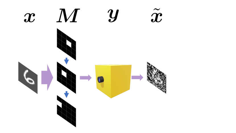
(a) Direct measurement strategy (Raster scan)

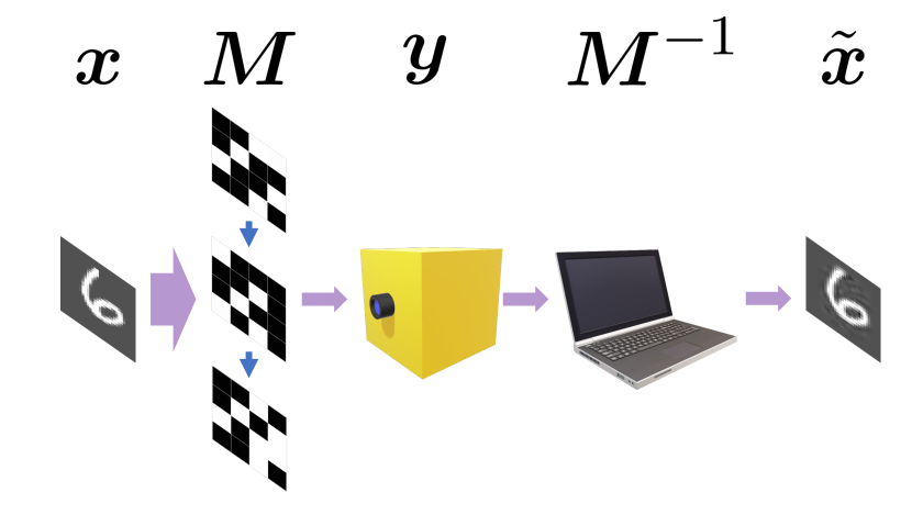
(b) Computational imaging strategy (Basis scan)

Figure 1: $\boldsymbol{x}$: object, $\boldsymbol{M}$: masks of coding, $\boldsymbol{y}$: counted photon numbers at the sensor, $\boldsymbol{M}^{-1}$: reconstruction operator, $\tilde{\boldsymbol{x}}$: reconstructed object. (LABEL:sub@fig:RasterScan) Only one pixel (white) is scanned in each measurement, and the measured data requires no reconstruction. (LABEL:sub@fig:BasisScan) The sum of all white pixels is measured in each measurement and it requires a decoding step to reconstruct the field of view.

III-A1 Coding Types

• Raster scan entails a pixel-wise scanning approach where photon counts for all pixels are sequentially measured. Mathematically, the sensing matrix $\boldsymbol{M}=\boldsymbol{I}$, an identical matrix.

• Impulse imaging entails an ideal camera that simultaneously captures complete hyper-spectral data. A prominent instance is a pixel array. When the field of view $\boldsymbol{x}$ consists of $N$ pixels, the sensing matrix assumes the form $\boldsymbol{M}=N\boldsymbol{I}$ where $\boldsymbol{I}$ is an identical matrix. Each pixel receives $N$ times the exposure in comparison to the raster scan scenario. This technique sets a benchmark akin to a gold standard, serving as an upper limit for the CI performance and an indicator of the noise level for comparison.

• Non-Selective Codes encompass coding schemes that lack adaptation to the inherent sparsity of a given dataset. Codes falling within this category are not crafted based on the statistical attributes of a representative training set. This classification encompasses a range of widely used codes, such as Hadamard patterns and Rademacher Random codes, which do not leverage the specific characteristics of the dataset. This grouping also extends to truncated Hadamard patterns, a popular choice in compressed sensing, which employ random subsets of complete Hadamard basis.

• Selective Codes. In this study, we elucidate the necessity for the tailored selection of codes in the context of single photon cameras to effectively capture sparse data representations. To address this, we harness both PCA codes and ONN-generated codes. Principal Component Analysis (PCA) serves as a classical technique for analyzing and classifying multispectral data correspondences [33, 34, 35, 36, 37]. Specifically, we compute the most significant components from training data and implement them as hardware masks within this project. The recorded photon counts, $\boldsymbol{y}$, are subsequently fed into a classifier to optimize the model. The Optical Neural Networks (ONN) approach mirrors a fully-connected neural network model, yet with its first hidden layer simulating the sensing matrix $\boldsymbol{M}$. By adeptly applying physical constraints to this foundational layer, the model becomes capable of determining the optimal sensing matrix for a designated task.

III-A2 Reconstruction Tasks

• Classic Imaging (Null-prior/No Compression): In tasks involving classic imaging, a null-prior is assumed, and there is no compression during measurements. The rank of the measurement matrix $\boldsymbol{M}$ is required to be equal to $N$, the number of pixels in the FOV. This scenario, such as in raster scan applications, is universal and does not necessitate prior knowledge of the FOV. Full-rank Hadamard matrices can be employed for reconstruction in noise-free situations. Common coding types for this task include raster scan and non-selective codes.

• Image Processing and Computational Imaging (Weak-prior/Some Compression): In this kind of tasks, a weak-prior assumption is made, allowing for some compression during measurements. This idea is based on prior knowledge, such as signals being sparse in some linear space, with noise concentrated in the high-frequency domain. An example is the JPEG format. If only the low-frequency components of Hadamard matrices are measured for reconstructing the FOV, this task is engaged. Non-selective codes are typically used for this purpose.

• Computer Vision (Strong-prior/Much Compression): Tasks related to computer vision involve a strong prior, enabling substantial compression during measurements. After reconstructing the FOV, the process often transitions to downstream computer vision tasks like classification. Alternatively, direct capture of principal features by $\boldsymbol{M}$ is possible if some of its components resemble the FOV. In these tasks, a few measurements are often sufficient with a strong prior derived from training data. Selective codes are commonly employed in this context.

III-B Constraints of sensing matrices

While we can identify the optimal $\boldsymbol{M}$ tailored to the tasks at hand, it’s crucial to acknowledge that the optimization problem for $\boldsymbol{M}$ might not exhibit convexity. This is attributed to the presence of two constraining factors. Consequently, achieving globally optimal masks may not be universally feasible within the scope of this problem.

1. Flux-preserving [1]. The single-pixel camera model involves the allocation of available photons among masks, as discussed in [17]. It is important to ensure that the mask basis $\boldsymbol{M}$ does not produce additional photons through improper entries [17]. Mathematically, $\sup\sum_{i=1}^{m}M_{ij}=1,\forall j\in\{1,2,\dots,N\}$ [17].

2. Positivity-preserving [1]. It is not possible to physically implement negative values for the masks $\boldsymbol{M}$, as demonstrated in [17, 1]. In this project, we employed the dual-rail approach as outlined in the work of Neifeld et al. [17].

III-C Model under Noise

This project investigates two noise models. The first one is the additive Gaussian noise (AGN) or read noise, which mainly originates from thermal vibrations of atoms at sensors. In this noise model, Eq. 1 becomes:

$$\tilde{\boldsymbol{y}}=\boldsymbol{Mx}+\boldsymbol{\epsilon},$$ (2)

where $\boldsymbol{\epsilon}\sim\mathcal{N}(\boldsymbol{0},\sigma^{2}\boldsymbol{I})$, and $\sigma$ is the standard deviation. The other noise model is the Poisson noise or shot noise, which arises from the statistical nature of photons [38]. The measurement equation for this noise model is:

$$\tilde{\boldsymbol{y}}\sim\mathcal{P}(\boldsymbol{Mx}).$$ (3)

It should be noted that the constraint 2 in Eq. 3 prohibits negative entries in $\boldsymbol{M}$.

IV Methods

IV-A Model Configuration

All coding strategies for classification tasks share the same fundamental model structure, as illustrated in Fig. 2. To classify handwritten numbers using optical devices with limited photon budget, we built a PyTorch-based pipeline consisting of a scanner module and a classifier module. The scanner module simulates the photon counting process using the techniques described in section III-A. For the classification task, we utilized a two-hidden layer artificial neural network (ANN) with 40 and 128 nodes, serving as the primary model. To prevent overfitting and enhance generalizability, we applied dropout after each hidden layer, followed by a rectified linear unit (ReLU) activation layer.

During the training of the model, the scanner computes the photon counts with noise and then transmits this data to the classifier. The noise is sampled from a pre-defined noise distribution and varies across epochs. Once the loss has been computed, gradient descent is used to optimize the parameters of the classifier. What sets the ONN apart from other models is that back-propagation is extended into the scanner, allowing for the simultaneous optimization of the masks and the classifier under different noise models. This approach offers distinct advantages compared to traditional methods, which typically optimize the classifier independently of the scanner or optimize the scanner without the appropriate noise model.

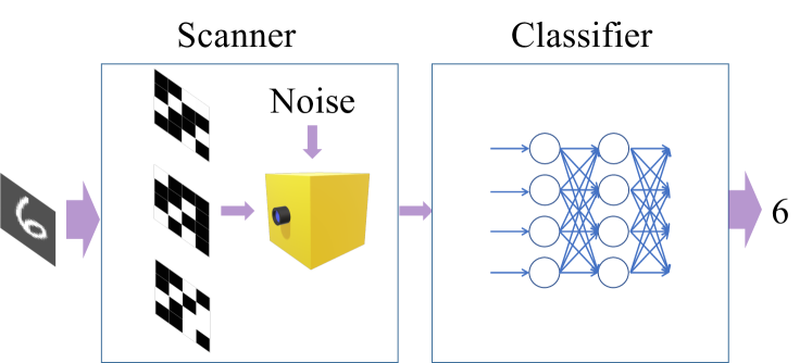
Figure 2: Model configuration

ONN can also be used for reconstruction. To address this, we propose a simple approach of optimizing the ONN masks for a reconstruction task under different noise models. To achieve this, we developed a new ONN model with $m=N$ masks. The scanner takes raw image vectors $\boldsymbol{x}$ and outputs $N$-element measured photon count vectors under a chosen noise model, $\tilde{\boldsymbol{y}}$. The classifier is a single-layer network that takes $\tilde{\boldsymbol{y}}$ as input and outputs $\tilde{\boldsymbol{x}}$, also an $N$-element vector. The objective is to minimize the MSE between the input images and the output vectors, $\|\tilde{\boldsymbol{x}}-\boldsymbol{x}\|_{2}^{2}$. In noiseless cases, the classifier is equivalent to $\boldsymbol{M}^{-1}$, where $\boldsymbol{M}$ is the masks used in the scanner.

ONN Optimization under Poisson Noise

Optimizing the scanner can be challenging as the Poisson noise generating function typically lacks a gradient. While reparameterization is a useful method for addressing AGN, it is not as effective for addressing Poisson noise. To address this limitation, we employ a method mentioned by Cossairt et al. that utilizes a normal distribution with a variance equal to its expectation to approximate the Poisson distribution during training [10]. This approximation enables us to employ PyTorch builtin reparameterization method, i.e. rsample, and optimize the scanner more effectively under Poisson noise.

To approximate the Poisson noise by the AGN, we can re-write the measurement with noise $\tilde{\boldsymbol{y}}=\boldsymbol{Mx}+\boldsymbol{J}$ where $\boldsymbol{J}=(\boldsymbol{Mx})^{\frac{1}{2}}\odot\boldsymbol{\epsilon},\boldsymbol{\epsilon}\sim\mathcal{N}(0,\boldsymbol{I})$. During the training under Poisson noise, $\boldsymbol{J}$ also plays a role in gradient computation, which is the most significant difference compared with training under the AGN.

IV-B Model Validation

To affirm the correctness of the ONN model, we initiate the validation process with a theoretical derivation of the null-prior reconstruction. Subsequently, we conduct empirical testing of the ONN model by reconstructing random signals under two distinct noise models. This experimental approach allows us to observe the convergence of optimized masks, providing empirical evidence for the validity and efficacy of the ONN model.

IV-B1 Theoretical Treatment for Null-Prior Reconstruction

Define $\boldsymbol{I}$ as the identity matrix and $\mathfrak{N}=\rho\tau$ as the total number of photons from the source. Given the noisy photon counts $\tilde{\boldsymbol{y}}$ and the full-rank mask basis $\boldsymbol{M}$, we can reconstruct the field of view $\tilde{\boldsymbol{x}}=\boldsymbol{M}^{-1}\tilde{\boldsymbol{y}}$. Based on Parseval’s identity, the covariance matrix of a vector $\boldsymbol{b}$ is $\boldsymbol{\Sigma}_{\boldsymbol{b}\boldsymbol{b}}=c^{2}\sigma^{2}\boldsymbol{I}$ if $\boldsymbol{b}=\boldsymbol{Wa}$ where $\boldsymbol{\Sigma}_{\boldsymbol{a}\boldsymbol{a}}=\sigma^{2}\boldsymbol{I}$ and $\boldsymbol{W}\boldsymbol{W}^{\top}=c^{2}\boldsymbol{I}$ . For RS, we have $\lambda=\frac{\mathfrak{N}}{N^{2}}$ and $\lambda\tilde{\boldsymbol{y}}\sim\mathcal{N}(\lambda\boldsymbol{I}\boldsymbol{x},\sigma^{2}\boldsymbol{I})$. Thus, the reconstructed field of view is

$$\begin{aligned} \tilde{\boldsymbol{x}}&\sim\mathcal{N}\left(\boldsymbol{x},\frac{\sigma^{2}N^{4}}{{\mathfrak{N}}^{2}}\boldsymbol{I}\right)\end{aligned}.$$ (4)

For HB, we have $\lambda=\frac{\mathfrak{N}}{2N^{2}}$ and $\lambda\tilde{\boldsymbol{y}}\sim\mathcal{N}(\lambda\boldsymbol{H}\boldsymbol{x},2\sigma^{2}\boldsymbol{I})$ due to the dual branch trick mentioned in section III-B. For $\boldsymbol{H}^{-1}$, $c=\sqrt{\frac{1}{N}}$. The reconstructed field of view is

$$\begin{aligned} \tilde{\boldsymbol{x}}&\sim\mathcal{N}\left(\boldsymbol{x},\frac{8\sigma^{2}N^{3}}{{\mathfrak{N}}^{2}}\boldsymbol{I}\right)\end{aligned}.$$ (5)

Therefore, using the Hadamard matrix in the AWGN model can improve the signal-to-noise ratio (SNR) of the reconstructed field of view when the number of elements, $N$, is large.

When the noise is Poisson distributed, the covariance matrix of the noisy photon counts depends on the choice of $\boldsymbol{M}$. Suppose $\sigma_{j}$ is the standard deviation of $\lambda\tilde{y}_{j}$, the $j_{\text{th}}$ measured noisy photon counts. For the RS, we have $\sigma_{j}^{2}=\lambda x_{j}$ and $\lambda=\frac{\mathfrak{N}}{N^{2}}$. The covariance matrix of the reconstructed field of view is thus

$$\begin{aligned} \boldsymbol{\Sigma}_{\tilde{\boldsymbol{x}}\tilde{\boldsymbol{x}}}&=\frac{N^{2}}{\mathfrak{N}}\text{diag}\{x_{1},x_{2},\cdots,x_{N}\}\end{aligned}.$$ (6)

In the case of the HB, we can express the rate parameter $\lambda$ as $\lambda=\frac{\mathfrak{N}}{2N^{2}}$, as demonstrated in section III-B using the Skellam Distribution. Additionally, we can express the variance of each element in the sum as $\sigma_{j}^{2}=\lambda\sum_{k=1}^{N}|H_{jk}|x_{k}$. As Hadamard matrices only contain entries of $\pm 1$, this reduces to $\sigma_{j}^{2}=\lambda\sum_{k=1}^{N}x_{k}$. Using this information, we can construct the covariance matrix

$$\begin{aligned} \boldsymbol{\Sigma}_{\tilde{\boldsymbol{x}}\tilde{\boldsymbol{x}}}&=\frac{2N\sum_{k=1}^{N}x_{k}}{\mathfrak{N}}\boldsymbol{I}\end{aligned}.$$ (7)

The results of our analysis reveal that the mean squared error (MSE) of the HB method is twice that of the RS method when the noise is Poisson distributed. This difference is attributed to the dual branch trick utilized in the HB method. Despite the use of two PMTs in the HB method, it is unable to surpass the reconstruction error of the RS method. These findings demonstrate the limitations of the HB method in comparison to the RS method under Poisson noise conditions.

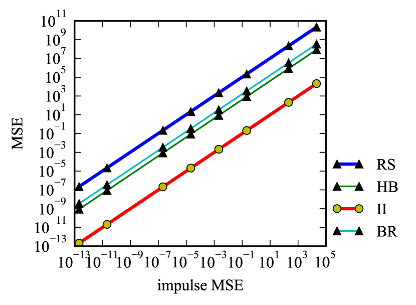
(a) Reconstruction under Gaussian noise

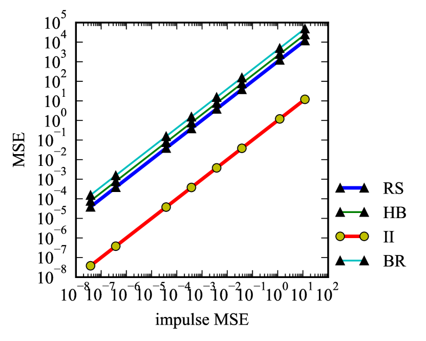
(b) Reconstruction under Poisson noise

Figure 3: Reconstruction errors on simulated data. RS: Raster basis. HB: Hadamard basis. II: Impulse imaging. BR: Binary random basis. (LABEL:sub@fig:gaussian_reconstruction) RS is always worse than HB for all noise levels under Gaussian noise. (LABEL:sub@fig:gaussian_reconstruction) HB is no better than RS under Poisson noise.

IV-B2 Mask optimized with ONN for Reconstruction

The primary question to address is whether the ONN has the ability to identify noise specific optimized masks. We established a benchmark by comparing the reconstruction performance in terms of mean squared error (MSE) between the original and reconstructed images, denoted by $\|\tilde{\boldsymbol{x}}-\boldsymbol{x}\|_{2}^{2}$, where $\tilde{\boldsymbol{x}}=\boldsymbol{M}^{-1}\tilde{\boldsymbol{y}}$. The reconstructed images were obtained using the Hadamard basis and Raster basis under Poisson noise and AGN models respectively. The outcomes, depicted in Fig. 3 where the x-axis is the log-scaled MSE of impulse imaging with different exposure times, indicate that the Hadamard basis is less effective in the presence of Poisson noise, while it is more effective under the AGN model when compared to the Raster basis. Given that many algorithms rely on the AGN model, their conclusions may not hold if the optimal masks differ under Poisson noise.

To make this reconstruction task less specific and more general, we reshaped the input data vectors $\boldsymbol{x}$ from $10^{5}$ random 8 by 8 patterns, increasing their generality. We randomly re-generated $\boldsymbol{x}$ for 10 times during the training, introducing additional variability. The simulations were conducted under significant noise, with a total of $1\times 10^{2}$ photons. We initialized the masks $\boldsymbol{M}$ with an $N\times N$ identical matrix and a $\{0,1\}$ Hadamard matrix respectively, and optimized them until the model reported constant losses.

Fig. 4 displays the first 6 optimized masks generated by the ONN model. A notable observation is that the model exhibits distinct behavior patterns under the AGN and Poisson noise. Specifically, it tends to open more pixels to enhance light throughput under the AGN, but adheres to the RS mode under the Poisson noise. Fig. 5 provides a more detailed visualization of the optimized masks by presenting the distribution of their entries. The x-axis represents the values in the masks, while the y-axis shows the total number of entries within a specific range. This observation aligns with the reconstruction results, where the RS performed modestly under the AGN but considerably better under the Poisson noise. The rationale behind this is that re-projection from a captured basis into a basis of sparsity does not yield the same recovery quality under Poisson noise that is provides for AGN. To obtain a performance benefit over the trivial point scanning method, or RS, it is essential that the data is sparse and is captured in a sparse basis. Since random patterns are not sparse, the best scanning strategy is the point scanning, which matches our results.

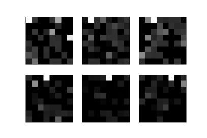
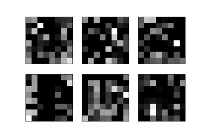
(a) ONN optimized masks under Gaussian noise. Left: initialized with the identity matrix. Right: initialized with the Hadamard matrix.

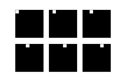
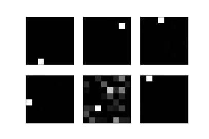
(b) ONN optimized masks under Poisson noise. Left: initialized with the identity matrix. Right: initialized with the Hadamard matrix.

Figure 4: First 6 optimized masks

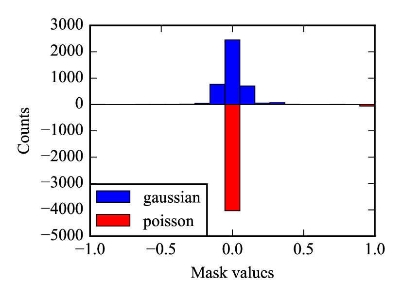
(a) $\boldsymbol{M}_{G}^{I}$ VS $\boldsymbol{M}_{P}^{I}$

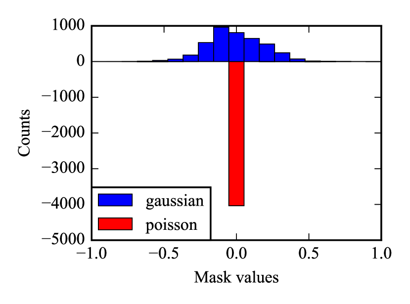
(b) $\boldsymbol{M}_{G}^{H}$ VS $\boldsymbol{M}_{P}^{H}$

Figure 5: The Poisson noise data is displayed topside-down by negating its counts. Let $\boldsymbol{M}_{G}^{I}$ represent masks initialized with the identity matrix and optimized under the AGN, and $\boldsymbol{M}_{P}^{I}$ denote masks initialized with the identity matrix and optimized under Poisson noise. Additionally, $\boldsymbol{M}_{G}^{H}$ and $\boldsymbol{M}_{P}^{H}$ represent masks initialized with the Hadamard matrix and optimized under AGN and Poisson noise, respectively. While $\boldsymbol{M}_{G}^{I}$ dynamically enhances light throughput by opening more pixels, $\boldsymbol{M}_{P}^{I}$ remains fixed, representing an already ideal choice. Notably, $\boldsymbol{M}_{P}^{H}$ tends to approach the identity matrix, in contrast to the behavior of $\boldsymbol{M}_{G}^{H}$. The challenge arises from the non-convex nature of this optimization problem, making it difficult for $\boldsymbol{M}_{P}^{H}$ to converge perfectly to the identity matrix. Nevertheless, this deviation underscores fundamental distinctions in optimizing masks under these distinct noise models.

The results from optimizing the masks indicate that the optimal masks under the AGN model may not perform similarly under Poisson noise. Specifically, methods developed under the AGN assumption may not be effective when the measured data follows a Poisson distribution. For instance, coding optimization based on minimizing the mutual coherence in compressed sensing [20] may be defective. The inherent differences in the underlying noise models of the two distributions can lead to suboptimal performance of AGN-optimized masks in Poisson noise scenarios. Therefore, it is crucial to consider Poisson noise when designing coding schemes and algorithms for imaging applications, especially when working with state-of-the-art sensors.

IV-C Computer Simulated Experiments

IV-C1 MNIST Simulated Data Preparation

The MNIST dataset, which comprises handwritten digits ranging from 0 to 9, has a default size of 28 by 28 pixels [39]. To align the data with Hadamard matrices, we added black pixels to the edges of the images and resized them to 32 by 32 pixels [39]. Subsequently, we rescaled the pixel values from the original range of $[0,1]$ to $[0.3,1]$. This rescaling was aimed at improving the dataset’s suitability for different noise models, as the initial black backgrounds do not introduce Poisson noise, which is typically proportional to the expected photon counts.

IV-C2 Spectral Datasets and Performance Evaluation

The model performances were assessed based on their average classification rates, which were calculated after five independent tests. In each test, the dataset was randomly split into 70% for training and 30% for validation. The model generated noisy photon counts during each assessment, and the training continued until the validation rate reached a plateau or declined. The highest validation rate obtained during the training process was considered as the representative upper bound for each assessment. The overall model performance was determined by averaging the results from all five assessments. This comprehensive evaluation ensured the reliability and accuracy of the model performance.

IV-D Hardware Experiments

To further support our conclusions, we conducted an experiment in addition to simulations. The experiment utilized a DMD (digital micromirror device), specifically the DLP 7000 model from Texas Instruments, and a PMT (photomultiplier tube) from PicoQuant, specifically the PMA Series. The experimental setup involved both hardware-end data acquisition and software-end classifier training.

To ensure that the classifier was accurately trained using the PMT data, we performed a transformation and re-calibration of the MNIST images to match what the PMT would actually ”observe” during data acquisition. This step is crucial when training the classifier without the use of hardware-end data. By implementing this transformation and re-calibration process, we were able to accurately simulate the imaging conditions that the PMT would encounter during actual data acquisition, allowing for more reliable and robust classification results.

First, we performed a Raster scan of a sample from the MNIST dataset, with each mask exposed for 1 second. The light intensity was adjusted to ensure that the brightest pixel generated approximately 1000 photon counts per second. The data captured during this experiment was then reshaped into a 32 by 32 image, which can be regarded as a linearly transformed version of the original raw image.

Figure 6: Raw image (left) VS measured image

Then, we estimated the linear transformation between the digital and experimental data to ensure that the digital data closely matched the sensor’s observations. After applying this transformation to all digital data, we used it to train the software-end classifier through simulation. Additionally, in this step, the masks used for Selective Sensing were also trained. The masks with decimals use the fraction of a super pixel [28] The ONN training is called in silico method (Wright et al) [28, 40]

After generating the mask pattern sequences, we uploaded them onto the DMD to acquire the data, denoted as $\tilde{\boldsymbol{y}}$. Our test set consisted of ten handwritten images, each of which appeared exactly once during the experiment. To control the noise level in the data, we varied lengths of random intervals throughout the 1-second exposure time for each mask. By preserving the arrival times of all photons, we were able to systematically adjust the level of noise in the acquired data.

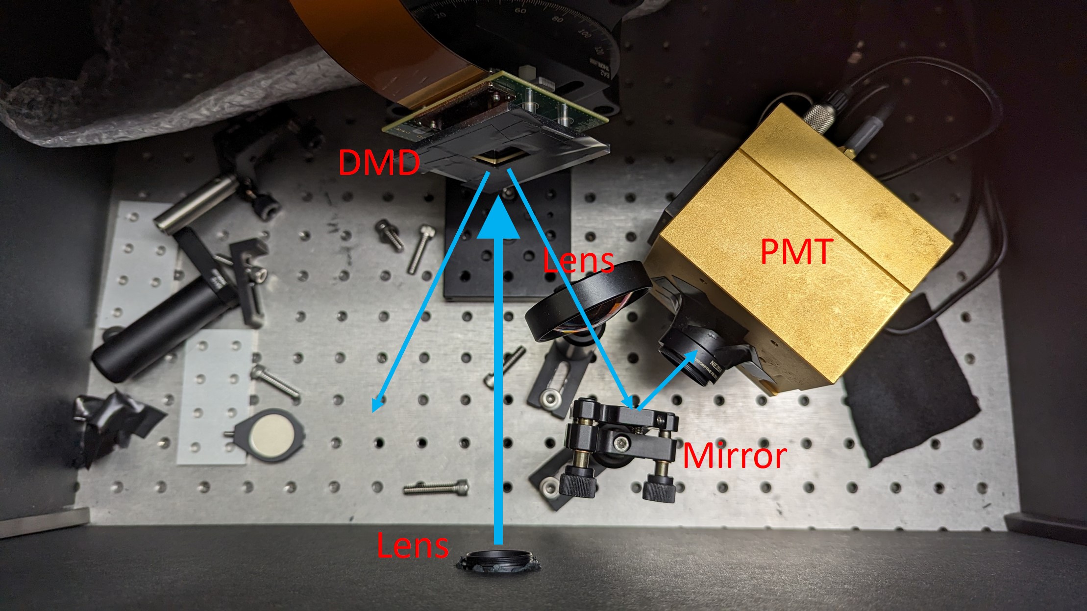
Figure 7: Experimental Configuration of the Single-Pixel Camera: The light path is illustrated by the blue arrows in the diagram. Specifically, our setup utilizes only one branch reflected by the DMD.

V Results

V-A Classification Rates on Simulated Experiment Data

We evaluated our proposed model through simulations that tested both AGN and Poisson noise models, using varying exposure times to generate results at different noise levels. We also tested all compressible strategies, varying the total number of masks, and defined a metric called compression ratio as the ratio of the number of masks to the number of pixels [41]. For RS and HB, this ratio was constrained to be 1.00, while the rest were evaluated over values in $\mathcal{C}_{R}=\{0.01,0.04,0.09,0.16,0.25,0.36,0.49,0.64,0.81,1.00\}$. Unlike pre-defined masks used by other strategies, the initial masks for ONN can affect performance in the presence of noise. We therefore initialized its masks with the PCA components from the training data, which typically yield better performance.

Figure 8 displays the classification performance of different parameters. The x-axis is the log-scaled MSE of impulse imaging (II) with varying exposure times. This MSE is the gold standard in this project and serves as a metric to measure the noise level for both AGN and Poisson noise models. The y-axis represents the validation set’s classification rate. We explored all the values in $\mathcal{C}_{R}$ to determine the best compression ratio for TH, PCA, and ONN since compression ratio affects classification performance. The figure shows the best results among all compression ratios for each strategy.

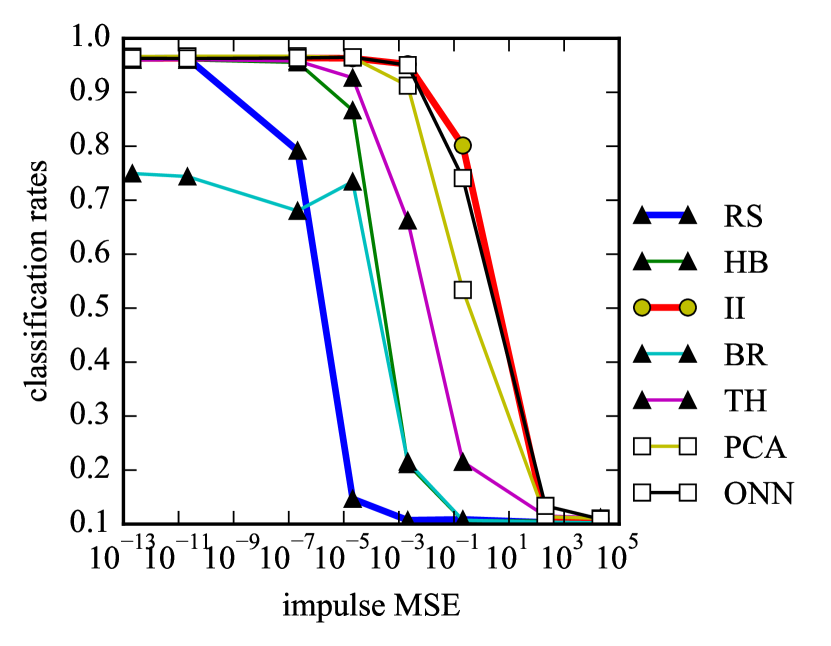
(a) Classification under Gaussian noise

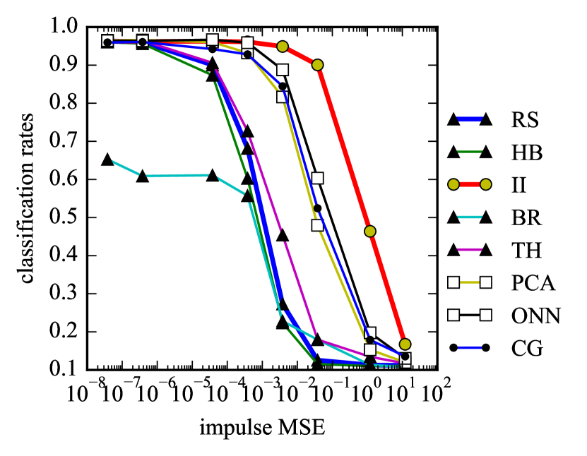
(b) Classification under Poisson noise

Figure 8: Classification rates on simulated data. RS: Raster basis. HB: Hadamard basis. II: Impulse imaging. BR: Binary random basis. TH: Truncated Hadamard basis. PCA: PCA basis. ONN: Optical Neural Networks. CG: control group. Selective strategies are marked by $\square$ and non-selective strategies are marked by $\blacktriangle$.(LABEL:sub@fig:gaussian_classification) RS is the worst but using other non-selective coding strategies can improve the performance under the AGN. (LABEL:sub@fig:poisson_classification) Among all non-selective strategies, only selective strategies can significantly improve the performance under Poisson noise. The CG employs the optimized masks under the AGN and trains the software classifier under Poisson noise. Its performance is worse than the ONN.

The results presented in the figure demonstrate that II consistently achieves the highest performance, which is in line with our expectations. In the presence of AGN, all coding schemes exhibit significant improvements over RS and in many cases provide adequate performance. This is because under Gaussian noise, projected from a captured basis into a basis of sparsity where the classifier operates can be done without a significant noise penalty. Moreover, for the classification task at hand, low-rank measurement techniques such as HB, PCA, and ONN, can yield further improvements in classification performance. Notably, the ONN approach produces results that are nearly as good as the II approach, while using only 0.1% of the photons.

However, when dealing with Poisson-distributed measured data, the effectiveness of Hadamard-based (HB) coding is no longer superior to that of RS. This aligns with the findings of Harwit et al. [6], which discourage the adoption of coding for Poisson noise. Despite this, there is still potential for performance improvement by utilizing low-rank methods such as TH, PCA and ONN. This is likely due to the fact that the images with analyze do in fact have sparsity in the Hadamard basis. Selective Sensing where capture patterns are optimized to capture sparsity directly like the ONN can retain their performance under poisson noise making them viable replacements for simple point scanners. This indicates that Selective Sensing is the most optimal approach for both noise models.

V-B Classification Performances on Hardware Experiment Data

In our experiments, we utilized a DMD and a PMT to measure ten handwritten digits from the MNIST dataset. To train the models, we employed $10^{5}$ photons, which constituted a higher noise level in comparison to the experimental setup. The collected data took the form of a series of timestamps recording the photons’ arrival time. During data collection, both RS and HB used 1024 masks, while the TH and HB employed the same measured data, but the TH used only the first 92 measurements. Similarly, PCA and ONN utilized 92 masks. Physical measurements took one second per mask for all strategies. To generate data with higher noise levels from the raw data, we randomly selected intervals within the 1-second span and counted the total number of photons within them. Since the ONN and PCA had only 92 masks, the maximum exposure time was set to 92 seconds. To ensure a fair comparison, we computed the interval length for each strategy as $\frac{\tau}{m}$, where $\tau$ represents the total exposure time under investigation, and $m$ denotes the number of masks used for each strategy.

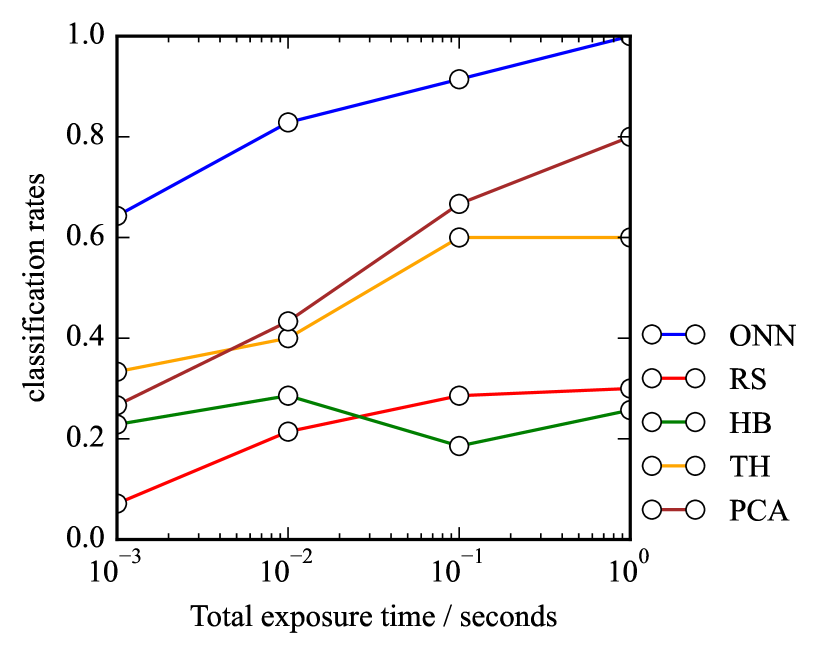
Figure 9: Classification rates on experiment data. RS: Raster basis. HB: Hadamard basis. TH: Truncated Hadamard basis. PCA: PCA basis. ONN: Optical Neural Networks. ONN is in general the best strategies given the experimental data.

Fig. 9 displays the classification rates achieved on the experimental data. The x-axis shows the exposure time, and the y-axis represents the classification rates of the models. Although there may be discrepancies between software training and hardware data acquisition, the ONN models performed excellently. However, the figure reveals some unexpected phenomena. Firstly, the HB strategy outperformed the RS for short exposure times, which was not observed in the simulations. This phenomenon may have arisen due to the dark photon in the PMT, a signal-independent noise that has about 40-80 counts per second, and was more pronounced in short exposures. Secondly, the TH achieved better classification performances than the PCA when the exposure time was short. This result was due to the use of unneeded PCA masks. To verify, we conducted simulations and made Fig. 10 by fixing the total number of photons at $10^{5}$ and varying the compression ratio under the Poisson noise. This figure showed that the PCA method could perform worse than the TH if extra masks were used. Hence, the PCA strategy requires careful estimation of the noise level to avoid using extra masks. Notably, the ONN appeared more stable when including extra masks, which is another advantage of the ONN. The ONN can perform robustly even with suboptimal numbers of masks, unlike the PCA strategy, which is noise-level sensitive. While it is possible to set the noise level during training, the effectiveness of the ONN can be evaluated for other levels of noise as well. This flexibility in application allows for broader use of the ONN beyond its specific training conditions, increasing its potential impact and utility in real-world scenarios.

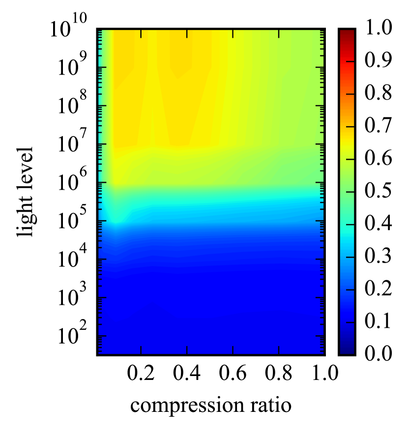
(a) Truncated Hadamard classification rate

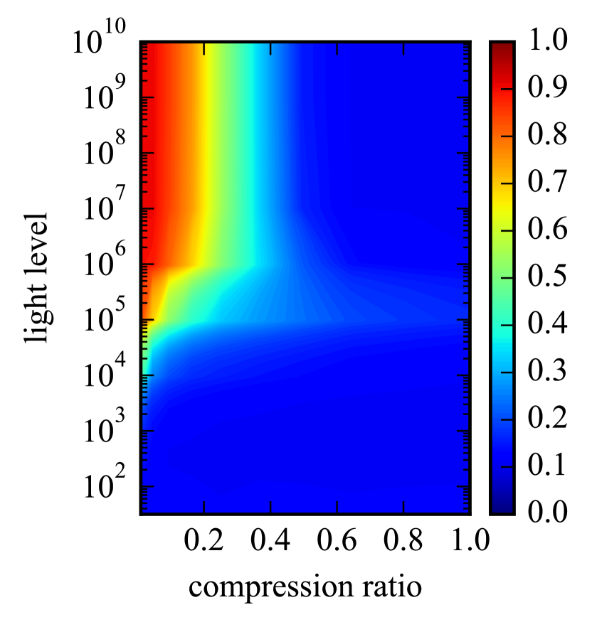
(b) Hardware PCA classification rate

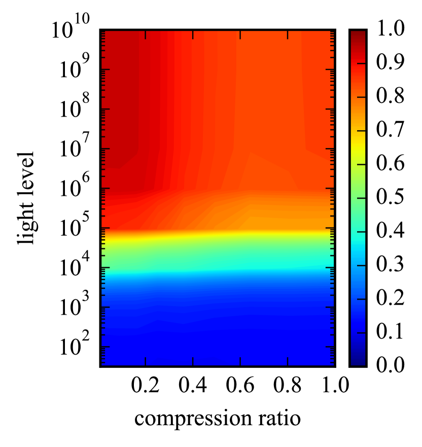
(c) ONN classification rate

Figure 10: Classification rates on simulated data w.r.t compression ratios and light levels. The models were trained using a light level of $10^{5}$ and subsequently tested under different light levels. It was observed that hardware PCA performance deteriorates when the compression ratio is not properly chosen, whereas the Truncated Hadamard and ONN models exhibit greater robustness in such scenarios.

V-C Simulated Experiment on Hyper-Spectral Data

In this experiment, we utilized the Indian Pines dataset [42], which was acquired through the Airborne Visible/Infrared Imaging Spectrometer (AVIRIS) on June 12, 1992, covering the Purdue University Agronomy farm northwest of West Lafayette and its surrounding area. Comprising $145\times 145$ pixels and 224 spectral reflectance bands in the wavelength range of 0.4 to 2.5 $\mu m$, this dataset provides a comprehensive view of the study area. Fig. 11 illustrates the classes within the Indian Pines dataset, presenting the counts associated with each class. The figure further features a representation of one channel (band 12) for all pixels, along with the ground truth of semantic labeling.

In this experiment, spectral data were zero-padded from 224 to 256 to align with the Hadamard mask and normalized to the range $[0,1]$. We utilized the scanner-classifier module from Fig. 2, adapting the ONN classification layers to the new dataset sizes. Each classification ran for 2000 epochs, with a learning rate of $5\times 10^{-3}$ and a batch size of 5000. Figure 13 illustrates the classification rates for the Indian Pines dataset across varying light levels from $10^{1}$ to $10^{10}$.

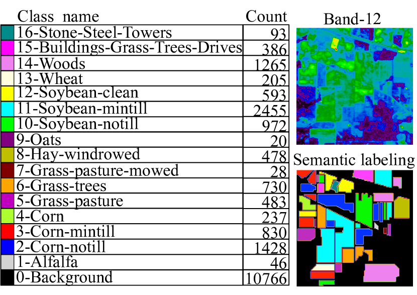
Figure 11: Indian Pines dataset [42]

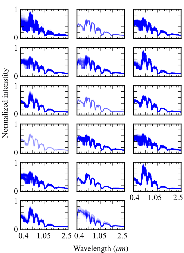
Figure 12: Spectrum for each class in the Indian Pines dataset

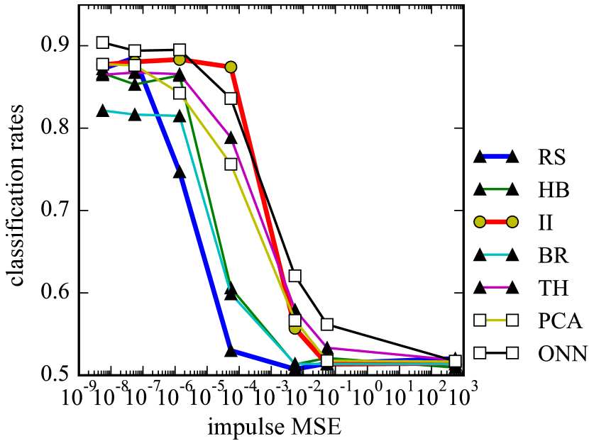
(a) Classification under Gaussian noise

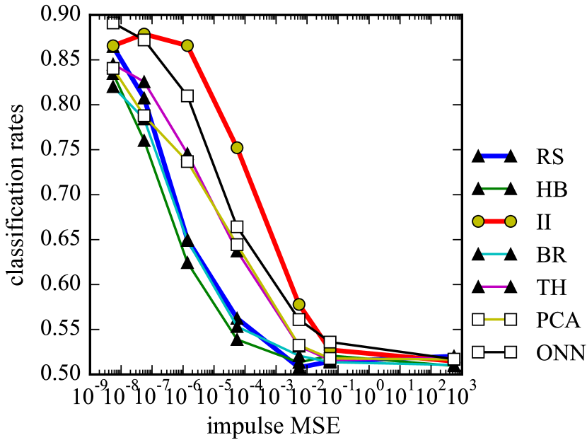
(b) Classification under Poisson noise

Figure 13: Classification rates of Indian Pines dataset varying light level. RS: Raster basis. HB: Hadamard basis. II: Impulse imaging. BR: Binary random basis. TH: Truncated Hadamard basis. PCA: PCA basis. ONN: Optical Neural Networks.

VI Discussion and Limitations

In compressed sensing and coding is typically defined as a measurement of an analog flux through some type of coding projection or in our example a mask. As has been shown by multiple works, this analog model of light does not account for the poisson noise inherent in any real measurements and leads to counter intuitive behavior of coding approaches.

If we instead think of our system as measuring photons through different codes, the code behavior makes intuitive sense. A photon measured through a mask with many open pixels carries less information about the scene than one captured through a raster mask because our measurement is ambiguous regarding which pixel in the mask was the origin of the photon. In a raster mask every photon can be uniquely assigned to one pixel. In essence, more photons do not equal more information.

The implication of this well documented problem become ever more important in the age of low noise and photon counting cameras where Poisson noise dominates all measurements. It is wide reaching since the projection process we study here in a specific coding experiment is part of the design of any camera. In other words: Any camera or vision system has to project data from a high dimensional scene space down into a lower dimensional sensor space where it encounters Poisson noise and then uses those noisy measurements to make inferences about the scene.

Our paper highlights the challenges of computational imaging under Poisson noise and its impact on algorithms based on the AGN noise assumption. We find that for compressible measurements, and especially tasks that involve direct feature extraction instead of signal reconstruction, a Selective Sensing approach using task optimized codes provides a viable coding solution. Through simulations and experiments, we demonstrate the feasibility of Selective Sensing and its promising classification performance on the MNIST handwritten number dataset. It is also robust in application scenarios with difficult-to-estimate noise levels. Our ONN method represents a method that can generate these selective measurements. Furthermore, Selective Sensing motivates the development of optical ANNs or ANNs with optical layers to globally optimize imaging systems.

Despite the promising results of our project, there are some limitations that must be acknowledged. First, we used a Gaussian noise model with reparameterization to train our model, which is only an approximation of the actual quantization noise at the sensor. Second, our test set consisted of only 10 numbers, which may not provide a comprehensive evaluation of the model’s performance. Additionally, we noted an inconsistency in that the model was trained using simulated data but tested with experimental data. Lastly, the Photon Distribution Factor rescales the masks $\boldsymbol{M}$, but its value changes during training and is not evolved during back-propagation. These limitations highlight the need for further improvements in the optimization of the ONN model, such as using more advanced optimization methods and larger sets of experimental data. Our work highlights the importance of the integration of imaging hardware and signal processing. In single photon accurate imaging systems, comprehensibility and sparsity of the data can be exploited to far greater effect during the measurement, as opposed to post processing.

References

- [1] M. Raginsky, R. M. Willett, Z. T. Harmany, and R. F. Marcia, “Compressed sensing performance bounds under poisson noise,” IEEE Transactions on Signal Processing, vol. 58, no. 8, pp. 3990–4002, 2010.
- [2] R. Raskar, “Computational photography: Epsilon to coded photography,” in Emerging Trends in Visual Computing: LIX Fall Colloquium, ETVC 2008, Palaiseau, France, November 18-20, 2008. Revised Invited Papers. Springer, 2009, pp. 238–253.
- [3] R. Foord, R. Jones, C. Oliver, and E. Pike, “The use of photomultiplier tubes for photon counting,” Applied optics, vol. 8, no. 10, pp. 1975–1989, 1969.
- [4] J. Prescott, “A statistical model for photomultiplier single-electron statistics,” Nuclear Instruments and Methods, vol. 39, no. 1, pp. 173–179, 1966. [Online]. Available: https://www.sciencedirect.com/science/article/pii/0029554X66900590
- [5] F. J. Lombard and F. Martin, “Statistics of electron multiplication,” Review of Scientific Instruments, vol. 32, no. 2, pp. 200–201, 1961.
- [6] M. Harwit and N. J. A. Sloane, Hadamard Transform Optics. Academic Press, 1979.
- [7] R. D. Swift, R. B. Wattson, J. A. Decker, R. Paganetti, and M. Harwit, “Hadamard transform imager and imaging spectrometer,” Applied optics, vol. 15, no. 6, pp. 1595–1609, 1976.
- [8] C. Scotté, F. Galland, and H. Rigneault, “Photon-noise: is a single-pixel camera better than point scanning? a signal-to-noise ratio analysis for hadamard and cosine positive modulation,” Journal of Physics: Photonics, vol. 5, no. 3, p. 035003, 2023.
- [9] W. Van den Broek, B. W. Reed, A. Béché, A. Velazco, J. Verbeeck, and C. T. Koch, “Various compressed sensing setups evaluated against shannon sampling under constraint of constant illumination,” IEEE Transactions on Computational Imaging, vol. 5, no. 3, pp. 502–514, 2019.
- [10] O. Cossairt, M. Gupta, and S. K. Nayar, “When does computational imaging improve performance?” IEEE transactions on image processing, vol. 22, no. 2, pp. 447–458, 2012.
- [11] A. Wuttig, “Optimal transformations for optical multiplex measurements in the presence of photon noise,” Appl. Opt., vol. 44, no. 14, pp. 2710–2719, May 2005. [Online]. Available: https://opg.optica.org/ao/abstract.cfm?URI=ao-44-14-2710
- [12] L. W. Schumann and T. S. Lomheim, “Infrared hyperspectral imaging fourier transform and dispersive spectrometers: comparison of signal-to-noise-based performance,” in Imaging Spectrometry VII, vol. 4480. SPIE, 2002, pp. 1–14.
- [13] N. Larson, R. Crosmun, and Y. Talmi, “Theoretical comparison of singly multiplexed hadamard transform spectrometers and scanning spectrometers,” Applied optics, vol. 13, no. 11, pp. 2662–2668, 1974.
- [14] L. Streeter, G. Burling-Claridge, M. Cree, and R. Künnemeyer, “Optical full hadamard matrix multiplexing and noise effects,” Applied Optics, vol. 48, no. 11, pp. 2078–2085, 2009.
- [15] D. Shin, J. H. Shapiro, and V. K. Goyal, “Performance analysis of low-flux least-squares single-pixel imaging,” IEEE Signal Processing Letters, vol. 23, no. 12, pp. 1756–1760, 2016.
- [16] R. Willett and M. Raginsky, “Poisson compressed sensing,” Defense Applications of Signal Processing, 2011.
- [17] H. S. Pal and M. A. Neifeld, “Multispectral principal component imaging,” Opt Express, vol. 11, no. 18, pp. 2118–25, 2003 Sep 8.
- [18] M. Neifeld and P. Shankar, “Feature-specific imaging,” Applied optics, vol. 42, pp. 3379–89, 07 2003.
- [19] A. Mahalanobis and M. Neifeld, “Optimizing measurements for feature-specific compressive sensing,” Applied Optics, vol. 53, no. 26, pp. 6108–6118, 2014.
- [20] M. Mordechay and Y. Y. Schechner, “Matrix optimization for poisson compressed sensing,” in 2014 IEEE Global Conference on Signal and Information Processing (GlobalSIP). IEEE, 2014, pp. 684–688.
- [21] S. Diamond, V. Sitzmann, F. Julca-Aguilar, S. Boyd, G. Wetzstein, and F. Heide, “Dirty pixels: Towards end-to-end image processing and perception,” ACM Transactions on Graphics (TOG), vol. 40, no. 3, pp. 1–15, 2021.
- [22] K. Zhang, J. Hu, and W. Yang, “Deep compressed imaging via optimized pattern scanning,” Photonics research, vol. 9, no. 3, pp. B57–B70, 2021.
- [23] C. Hinojosa, J. C. Niebles, and H. Arguello, “Learning privacy-preserving optics for human pose estimation,” in Proceedings of the IEEE/CVF international conference on computer vision, 2021, pp. 2573–2582.
- [24] X. Dun, H. Ikoma, G. Wetzstein, Z. Wang, X. Cheng, and Y. Peng, “Learned rotationally symmetric diffractive achromat for full-spectrum computational imaging,” Optica, vol. 7, no. 8, pp. 913–922, 2020.
- [25] C. A. Metzler, H. Ikoma, Y. Peng, and G. Wetzstein, “Deep optics for single-shot high-dynamic-range imaging,” in Proceedings of the IEEE/CVF Conference on Computer Vision and Pattern Recognition, 2020, pp. 1375–1385.
- [26] J. Chang and G. Wetzstein, “Deep optics for monocular depth estimation and 3d object detection,” in Proceedings of the IEEE/CVF International Conference on Computer Vision, 2019, pp. 10 193–10 202.
- [27] E. Onzon, F. Mannan, and F. Heide, “Neural auto-exposure for high-dynamic range object detection,” in Proceedings of the IEEE/CVF conference on computer vision and pattern recognition, 2021, pp. 7710–7720.
- [28] J. Spall, X. Guo, and A. I. Lvovsky, “Hybrid training of optical neural networks,” Optica, vol. 9, no. 7, pp. 803–811, Jul 2022. [Online]. Available: https://opg.optica.org/optica/abstract.cfm?URI=optica-9-7-803
- [29] E. Tseng, A. Mosleh, F. Mannan, K. St-Arnaud, A. Sharma, Y. Peng, A. Braun, D. Nowrouzezahrai, J.-F. Lalonde, and F. Heide, “Differentiable compound optics and processing pipeline optimization for end-to-end camera design,” ACM Transactions on Graphics (TOG), vol. 40, no. 2, pp. 1–19, 2021.
- [30] J. D. Rego, H. Chen, S. Li, J. Gu, and S. Jayasuriya, “Deep camera obscura: an image restoration pipeline for pinhole photography,” Optics Express, vol. 30, no. 15, pp. 27 214–27 235, 2022.
- [31] M. F. Duarte, M. A. Davenport, D. Takhar, J. N. Laska, T. Sun, K. F. Kelly, and R. G. Baraniuk, “Single-pixel imaging via compressive sampling,” IEEE Signal Processing Magazine, vol. 25, no. 2, pp. 83–91, 2008.
- [32] T. Wang, S.-Y. Ma, L. G. Wright, T. Onodera, B. C. Richard, and P. L. McMahon, “An optical neural network using less than 1 photon per multiplication,” Nature Communications, vol. 13, no. 1, p. 123, 2022.
- [33] C. Rodarmel and J. Shan, “Principal component analysis for hyperspectral image classification,” Surveying and Land Information Science, vol. 62, no. 2, pp. 115–122, 2002.
- [34] J. R. Carr and K. Matanawi, “Correspondence analysis for principal components transformation of multispectral and hyperspectral digital images,” Photogrammetric engineering and remote sensing, vol. 65, no. 8, pp. 909–914, 1999.
- [35] J. R. Jensen et al., Introductory digital image processing: a remote sensing perspective. Prentice-Hall Inc., 1996, no. Ed. 2.
- [36] R. C. Gonzales and P. Wintz, Digital image processing. Addison-Wesley Longman Publishing Co., Inc., 1987.
- [37] R. A. Schowengerdt, Remote sensing: models and methods for image processing. Elsevier, 2006.
- [38] A. K. Boyat and B. K. Joshi, “A review paper: Noise models in digital image processing,” ArXiv, vol. abs/1505.03489, 2015.
- [39] Y. Lecun, L. Bottou, Y. Bengio, and P. Haffner, “Gradient-based learning applied to document recognition,” Proceedings of the IEEE, vol. 86, no. 11, pp. 2278–2324, 1998.
- [40] L. G. Wright, T. Onodera, M. M. Stein, T. Wang, D. T. Schachter, Z. Hu, and P. L. McMahon, “Deep physical neural networks trained with backpropagation,” Nature, vol. 601, no. 7894, pp. 549–555, 2022.
- [41] R. Stojek, A. Pastuszczak, P. Wróbel, and R. Kotyński, “Single pixel imaging at high pixel resolutions,” Optics Express, vol. 30, no. 13, pp. 22 730–22 745, 2022.
- [42] M. F. Baumgardner, L. L. Biehl, and D. A. Landgrebe, “220 band aviris hyperspectral image data set: June 12, 1992 indian pine test site 3,” Sep 2015. [Online]. Available: https://purr.purdue.edu/publications/1947/1
Acknowledgment
The authors would like to thank…