ALMA 0.5 kpc Resolution Spatially Resolved Investigations of Nuclear Dense Molecular Gas Properties in Nearby Ultraluminous Infrared Galaxies Based on HCN and HCO⁺ Three Transition Line Data

Abstract

We present the results of our ALMA $\lesssim$0.5 kpc-resolution dense molecular line (HCN and HCO⁺ J=2–1, J=3–2, and J=4–3) observations of 12 nearby (ultra)luminous infrared galaxies ([U]LIRGs). After matching beam sizes of all molecular line data to the same values in all (U)LIRGs, we derive molecular line flux ratios, by extracting spectra in the central 0.5, 1, 2 kpc circular regions, and 0.5–1 and 1–2 kpc annular regions. Based on non-LTE model calculations, we quantitatively confirm that the innermost ($\lesssim$0.5 kpc) molecular gas is very dense ($\gtrsim$10⁵ cm^-3) and warm ($\gtrsim$300 K) in ULIRGs, and that in one LIRG is also modestly dense (10^4-5 cm^-3) and warm ($\sim$100 K). We then investigate the spatial variation of the HCN-to-HCO⁺ flux ratios and high-J to low-J flux ratios of HCN and HCO⁺. A subtle sign of decreasing trend of these ratios from the innermost ($\lesssim$0.5 kpc) to outer nuclear (0.5–2 kpc) region is discernible in a significant fraction of the observed ULIRGs. For two AGN-hosting ULIRGs which display the trend most clearly, we find based on a Bayesian approach that the HCN-to-HCO⁺ abundance ratio and gas kinetic temperature systematically increase from the outer nuclear to the innermost region. We suggest that this trend comes from potential AGN effects, because no such spatial variation is found in a starburst-dominated LIRG.

1 Introduction

Ultraluminous infrared galaxies (ULIRGs) radiate very strong infrared emission with luminosity L_IR $\gtrsim$ 10¹²L_⊙ and are usually seen as gas-rich galaxy major mergers in the nearby universe at $z<$ 0.3 (e.g., Sanders & Mirabel, 1996). The observed infrared luminosity is much higher than UV–optical luminosity in most cases, suggesting that the bulk of UV–optical emission from luminous, but hidden, energy sources is absorbed by dust which re-emits the absorbed energy as infrared thermal radiation. Through galaxy merger processes, a large amount of molecular gas and dust can concentrate into nuclear regions ($\lesssim$1–2 kpc). Star-formation (= starburst) activity and mass-accretion onto existing supermassive black holes (SMBHs), the so-called active galactic nucleus (AGN) activity, can occur there. Both the starburst and AGN activity can be the luminous hidden energy sources of ULIRGs, but distinguishing the relative energetic contribution of these two kinds of activity is not an easy task, because of huge dust extinction toward the hidden energy sources. Observations at wavelengths of strong penetrating power against dust are indispensable to scrutinize what is happening at nearby ULIRGs’ nuclei.

In the (sub)millimeter wavelength range at 0.3–3.5 mm where dust extinction effects are very small (Hildebrand, 1983), many rotational J-transition lines of abundant molecules are found. At nearby merging ULIRGs’ nuclei, the bulk of molecular gas is thought to be in a dense form ($\gtrsim$10⁴ cm^-3) (e.g., Gao & Solomon, 2004). For this reason, observations of (sub)millimeter rotational J-transition emission lines of dense molecular gas tracers with high dipole moments and/or high critical density can provide important information about the enigmatic nature of nearby ULIRGs’ nuclei. In fact, a starburst (= energy release by nuclear fusion inside stars) and an AGN (= radiative energy generated by a mass accreting SMBH) can have different physical and chemical effects to surrounding dense molecular gas, so that particular molecular emission lines can be strong depending on energy sources. Regarding the widely used bright CO emission lines, high-J (J $\gtrsim$ 4–5) ones can probe dense (and warm) molecular gas at nearby ULIRGs’ nuclei because of higher critical density (and excitation energy) than low-J (J=1–2) ones. Because it is theoretically predicted that high-J CO emission lines, relative to low-J CO ones, can be stronger in an AGN than in a starburst (e.g., Meijerink et al., 2007; Spaans & Meijerink, 2008), detection of significantly stronger high-J CO emission than that explained by starburst activity, has been used to argue for the presence of a luminous AGN (e.g., van der Werf et al., 2010; Spinoglio et al., 2012; Pereira-Santaella et al., 2014; Mashian et al., 2015; Lu et al., 2017; Esposito et al., 2022), with a caution that mechanical heating by shocks could also produce strong high-J CO emission lines (e.g., Hailey-Dunsheath et al., 2012; Meijerink et al., 2013; Pellegrini et al., 2013; Rosenberg et al., 2015; Kamenetzky et al., 2016).

Additionally, an AGN can enhance the abundance of some particular molecules, compared to a starburst, because stronger X-ray emission, when normalized to UV luminosity, and a larger amount of hot ($>$100 K) dust in an AGN, can make chemistry significantly different from a starburst (e.g., Meijerink et al., 2007; Harada et al., 2013). It is desirable to see how dense molecular emission line flux ratios differ between known starburst-dominated and AGN-important galaxies. HCN and HCO⁺ rotational J-transition line observations have been conducted before to probe dense molecular gas in nearby ULIRGs, because (1) the dipole moments of HCN and HCO⁺ are much larger than the widely used CO (Shirley, 2015) and (2) HCN and HCO⁺ are one of the brightest lines among putative dense molecular gas tracers (e.g., Martin et al., 2011; Aladro et al., 2011, 2015). However, these observations were done with large beams ($\gtrsim$5^′′ or $\gtrsim$5 kpc at $z\gtrsim$ 0.05) using single dish (sub)millimeter telescopes (e.g., Gao & Solomon, 2004; Baan et al., 2008; Gracia-Carpio et al., 2008; Krips et al., 2008; Greve et al., 2009; Costagliola et al., 2011; Papadopoulos et al., 2014; Privon et al., 2015; Ueda et al., 2021; Zhou et al., 2022; Israel, 2023) or pre-ALMA interferometric facilities with limited angular resolution of $\gtrsim$1$\farcs$5 (e.g., Imanishi et al., 2006b, 2007b, 2009a). Physical and chemical conditions at the energetically dominant nearby ULIRGs’ nuclei ($\lesssim$1–2 kpc) (e.g., Soifer et al., 2000; Diaz-Santos et al., 2010; Imanishi et al., 2011; Pereira-Santaella et al., 2021) may not be best probed with previously taken large-beam-sized observational data, because of possible contamination from spatially extended ($\gtrsim$a few kpc) molecular gas emission in the host galaxies.

With the advent of ALMA, conducting sensitive high-angular-resolution ($\lesssim$1^′′) dense molecular J-transition line observations in the (sub)millimeter has routinely become possible. Sub-arcsecond and sub-kpc-resolution HCN and HCO⁺ line observations of the two nearby well-studied ULIRGs Arp 220 ($z=$ 0.018) and Mrk 231 ($z=$ 0.042) were conducted (e.g., Scoville et al., 2015; Aalto et al., 2015a, b; Martin et al., 2016; Sakamoto et al., 2021). In Arp 220, dense molecular gas properties were investigated, using multiple J-transition molecular line data and non-LTE modeling (e.g., Tunnard et al., 2015; Sliwa & Downes, 2017; Manohar & Scoville, 2017). However, our understanding of dense molecular gas properties in nearby ULIRGs’ nuclei in general is still highly incomplete. Sub-arcsec ($\lesssim$a few kpc)-resolution HCN and HCO⁺ observational results of multiple nearby ULIRGs at J=2–1, J=3–2 and J=4–3 lines have been reported (e.g., Imanishi & Nakanishi, 2013a, b, 2014; Imanishi et al., 2016a, b, 2018, 2021, 2022). By combining these multiple J-transition HCN and HCO⁺ line data and by applying non-LTE model calculations, Imanishi et al. (2023) derived nuclear dense molecular gas properties of ten nearby (U)LIRGs at 1–2 kpc physical resolution. However, possible spatial variation of the properties within nearby ULIRGs’ nuclei cannot be investigated in detail with this resolution.

Imanishi et al. (2019) obtained $\lesssim$0$\farcs$2-resolution HCN and HCO⁺ J=3–2 observational data of $>$20 nearby ULIRGs at $z<$ 0.15. The corresponding physical scale is $\lesssim$0.5 kpc, which enables us to investigate dense molecular gas properties at $\lesssim$0.5 kpc spatial resolution within nearby ULIRGs’ nuclei, if multiple J-transition line data with similar resolution are available. By adding $\lesssim$0.5 kpc-resolution HCN and HCO⁺ J=2–1 and J=4–3 line data to the existing J=3–2 data, we will be able to obtain three independent J-transition line data. They can be used to better constrain the possible spatial variation of (1) physical properties of dense molecular gas, based on excitation conditions (high-J to low-J flux ratios) of both HCN and HCO⁺, and (2) chemical properties, by comparing HCN and HCO⁺ emission line fluxes at the same J-transition.

In this paper, we present our new $\lesssim$0$\farcs$2 ($\lesssim$0.5 kpc)-resolution HCN and HCO⁺ J=2–1 and J=4–3 observational results of nearby ULIRGs already observed at J=3–2 with similarly high spatial resolution by Imanishi et al. (2019). After matching beam sizes of multiple J-transition line data of both HCN and HCO⁺ to the same value, we attempt to investigate, with an aid of non-LTE calculations, (1) physical and chemical properties of nuclear dense molecular gas in a larger number of nearby ULIRGs, compared to the previous study by Imanishi et al. (2023), and (2) for the first time, how the properties spatially change between the innermost ($\lesssim$0.5 kpc) and outer nuclear (0.5–2 kpc) regions. Throughout this paper, (1) we adopt the cosmological parameters, H₀ $=$ 71 km s^-1 Mpc^-1, $\Omega_{\rm M}$ = 0.27, and $\Omega_{\rm\Lambda}$ = 0.73, (2) maps are shown in the ICRS coordinate, and (3) flux ratios of HCN-to-HCO⁺ and between different J-transition lines are calculated in units of Jy km s^-1. Density and temperature mean, respectively, H₂ volume number density (n${}_{\rm H_{2}}$) and kinetic temperature (T_kin), unless otherwise stated.

2 Targets

Our targets are originally selected from nearby ULIRGs in the well-studied IRAS 1 Jy sample (Kim & Sanders, 1998). We limit our sample to ULIRGs which are (1) at $z<$ 0.15, (2) at declination $<$ $+$20^∘ (to be best observable from the ALMA site in Chile), and (3) classified optically as LINERs or HII-regions (i.e., non-Seyferts; no obvious optical AGN signature), to investigate optically elusive, but intrinsically luminous buried AGNs. Imanishi et al. (2019) observed 26 such ULIRGs (a complete sample with expected dense molecular line peak flux above a certain threshold), at HCN and HCO⁺ J=3–2, with $\lesssim$0.5 kpc resolution in most cases, in ALMA Cycle 5. After excluding ULIRGs with too faint dense molecular emission lines (HCN J=3–2 peak flux from the central $\lesssim$0.5 kpc region is $\lesssim$1.5 mJy) and/or small ($\lesssim$1) HCN-to-HCO⁺ J=3–2 flux ratios (i.e., no signature of luminous buried AGNs; Imanishi et al. (2016b)), 16 ULIRGs were selected and their HCN and HCO⁺ J=2–1 and J=4–3 observations, at $\lesssim$0.5 kpc resolution, were proposed in ALMA Cycle 7. Not all the proposed ULIRGs were observed, due to limited observing time available, resulting in 11 observed ULIRGs. In addition to these ULIRGs, NGC 1614 (a starburst-dominated luminous infrared galaxy [LIRG] with L_IR = 10^11.7L_⊙ at $z=$ 0.016) is added for comparison, because J=2–1, J=3–2, and J=4–3 data of HCN and HCO⁺ with $\lesssim$0.5 kpc resolution are available (Imanishi & Nakanishi, 2013a; Imanishi et al., 2016b, 2022). Table 1 summarizes these (U)LIRGs studied in this paper. The 11 ULIRGs are not statistically complete and are possibly biased to AGN-important ULIRGs because sources with high ($\gtrsim$1) HCN-to-HCO⁺ J=3–2 flux ratios are selected (Imanishi et al., 2016b). However, we will be able to obtain valuable information on nuclear dense molecular gas properties in an increased number of nearby ULIRGs, because the observed sources are largely different from those studied by Imanishi et al. (2023).

Table 1: Basic Properties of the Observed (Ultra)luminous Infrared Galaxies

Object	Redshift	dL	Scale	f12	f25	f60	f100	log LIR	Optical	AGN	IR/submm/X
		[Mpc]	[kpc/′′]	[Jy]	[Jy]	[Jy]	[Jy]	[L⊙]	Class	IR [%]	AGN
(1)	(2)	(3)	(4)	(5)	(6)	(7)	(8)	(9)	(10)	(11)	(12)
IRAS 00091$-$0738	0.1180	543	2.1	$<$0.07	0.22	2.63	2.52	12.3	HII	58$\pm$6	Yb,c
IRAS 00188$-$0856	0.1285	596	2.3	$<$0.12	0.37	2.59	3.40	12.4	LINER	35$\pm$4	Yb,c,d,e
IRAS 00456$-$2904	0.1100	504	2.0	$<$0.08	0.14	2.60	3.38	12.2	HII	$<$0.05	Y
IRAS 01166$-$0844	0.1172	539	2.1	0.07	0.17	1.74	1.42	12.1	HII	88${}^{+6}_{-10}$	Yb,c,e
IRAS 01569$-$2939	0.1402	655	2.5	$<$0.11	0.14	1.73	1.51	12.3	HII	18$\pm$3	Yb
IRAS 03250$+$1606	0.1286	596	2.3	$<$0.10	$<$0.15	1.38	1.77	12.1	LINER	$<$0.2	Yd
IRAS 10378$+$1108	0.1365	636	2.4	$<$0.11	0.24	2.28	1.82	12.3	LINER	14$\pm$2	Yb,c,d
IRAS 16090$-$0139	0.1334	621	2.4	0.09	0.26	3.61	4.87	12.6	LINER	24$\pm$3	Yb,c,d,e
IRAS 22206$-$2715	0.1320	614	2.3	$<$0.10	$<$0.16	1.75	2.33	12.2	HII	$<$0.5	Y
IRAS 22491$-$1808	0.0776	347	1.5	0.05	0.55	5.44	4.45	12.2	HII	$<$0.07	Yf
IRAS 12112$+$0305	0.0730	326	1.4	0.12	0.51	8.50	9.98	12.3	LINER	$<$0.7	Yf,g (NE nucleus)
NGC 1614	0.0160	68	0.32	1.38	7.50	32.12	34.32	11.7	HII	$<$5

Note. — Col.(1): Object name. IRAS 12112$+$0305 is listed separately, because we have only one J-transition line data with $\lesssim$0.5 kpc resolution. Col.(2): Redshift adopted from ALMA dense molecular line data (Imanishi et al., 2016b), which are slightly different from optically derived ones (Kim & Sanders, 1998) in some cases. Col.(3): Luminosity distance in Mpc. Col.(4): Physical scale in kpc arcsec^-1. Col.(5)–(8): f₁₂, f₂₅, f₆₀, and f₁₀₀ are IRAS fluxes at 12 $\mu$m, 25 $\mu$m, 60 $\mu$m, and 100 $\mu$m, respectively, taken from Kim & Sanders (1998) or Sanders et al. (2003) or the IRAS Faint Source Catalog (FSC). Col.(9): Decimal logarithm of infrared (8$-$1000 $\mu$m) luminosity in units of solar luminosity (L_⊙), calculated with $L_{\rm IR}=2.1\times 10^{39}\times$ D(Mpc)² $\times$ (13.48 $\times$ $f_{12}$ + 5.16 $\times$ $f_{25}$ + $2.58\times f_{60}+f_{100}$) ergs s^-1 (Sanders & Mirabel, 1996). Col.(10): Optical spectroscopic classification by Veilleux et al. (1999) or Veilleux et al. (1995). “LINER” and “HII” refer to LINER and HII-region, respectively. Col.(11): Infrared spectroscopically estimated bolometric contribution of AGN in % by Nardini et al. (2010) for all ULIRGs and by Pereira-Santaella et al. (2015) for the LIRG NGC 1614. Col.(12): “Y” means the presence of the signatures of optically elusive, but intrinsically luminous buried AGNs. All ULIRGs show elevated ($\gtrsim$1) HCN-to-HCO⁺ J=3–2 flux ratios at $\sim$1.3 mm (Imanishi et al., 2019), possible signatures of luminous AGNs (e.g., Imanishi et al., 2016b). Other representative references for AGN signatures in the infrared 3–40 $\mu$m and/or (sub)millimeter spectra: ^b: Imanishi et al. (2007a). ^c: Veilleux et al. (2009). ^d: Imanishi et al. (2006a). ^e: Imanishi et al. (2010b). ^f: Imanishi et al. (2018). ^g: Imanishi et al. (2016b).

3 Observations and Data Analysis

Our HCN and HCO⁺ J=2–1 and J=4–3 observations of the 11 ULIRGs were conducted in our ALMA Cycle 7 program 2019.1.00027.S (PI = M. Imanishi). We employed the widest 1.875 GHz mode with 1920 channels for each spectral window. HCN and HCO⁺ lines were simultaneously observed in one sideband (LSB or USB). For IRAS 22206$-$2715 and IRAS 22491$-$1808, although HCN and HCO⁺ J=3–2 data were taken in ALMA Cycle 5 (Imanishi et al., 2019), the achieved beam sizes were much larger than $\sim$0.5 kpc, unlike other ULIRGs. For these two ULIRGs, we thus took $\lesssim$0.5 kpc-resolution HCN and HCO⁺ J=3–2 data as well. Table 2 tabulates our ALMA Cycle 7 observation log. For nine ULIRGs except IRAS 10378$+$1108 and IRAS 12112$+$0305, both J=2–1 and J=4–3 data of HCN and HCO⁺ were obtained, and so after combining with available or newly taken J=3–2 data, we have full three J-transition HCN and HCO⁺ data with $\lesssim$0.5 kpc resolution. For IRAS 10378$+$1108, we obtained only J=2–1 data in our ALMA Cycle 7 program and so can combine $\lesssim$0.5 kpc-resolution J=2–1 and J=3–2 data only. For IRAS 12112$+$0305, only J=4–3 data were taken in our ALMA Cycle 7 program. Because available J=3–2 data of IRAS 12112$+$0305 are not of sufficiently small physical resolution ($>$0.5 kpc) (Imanishi et al., 2019), we will only display newly taken J=4–3 data of the primary north-eastern (NE) nucleus (whose beam sizes are much smaller than previously published J=4–3 data by Imanishi et al. (2018)), but will not constrain nuclear dense molecular gas properties with $\lesssim$0.5 kpc resolution in detail.

We started our analysis from pipeline-calibrated data, using the CASA version 6.1.1.15 (The CASA Team, 2022), provided by ALMA. By choosing channels without showing obvious emission and absorption lines, we determined the continuum level, and subtracted it using the CASA task “uvcontsub”. Then we applied the “tclean” task (Briggs-weighting; robust $=$ 0.5 and gain $=$ 0.1) for the continuum-only and continuum-subtracted dense molecular line data to create cleaned maps. The final velocity resolution was $\sim$20 km s^-1 and the pixel scale was 0$\farcs$02 pixel^-1. According to the ALMA Cycle 7 Technical Handbook (equation 7.6) , the maximum recoverable scale (MRS) is $>$4^′′ at $\sim$0.85–2 mm (i.e., the wavelength range of HCN and HCO⁺ J=2–1, J=3–2, and J=4–3) for the minimum baseline length of 15–29 m (Table 2). This MRS corresponds to $>$5 kpc for all the observed ULIRGs, so that our targeting dense molecular line emission at ULIRGs’ nuclei ($\lesssim$1–2 kpc) should be fully recovered. This is also the case for the HCN and HCO⁺ J=3–2 data of ULIRGs taken in ALMA Cycle 5 (Imanishi et al., 2019). For the nearest LIRG NGC 1614 ($z=$ 0.016; 0.32 kpc arcsec^-1), molecular line emission with $\sim$1 kpc physical scale can be safely recovered with our ALMA data taken before Cycle 5. Because the J=2–1, J=3–2, and J=4–3 data were obtained at different times, we will take into account the possible absolute flux calibration uncertainty in individual ALMA observations, with maximum $\sim$5% for J=2–1 and $\sim$10% for J=3–2 and J=4–3 (ALMA Cycle 5 and 7 Proposer’s Guide) when we discuss molecular gas properties based on the flux comparison at different J-transitions. However, because HCN and HCO⁺ data at each J-transition were taken simultaneously, the HCN-to-HCO⁺ flux ratios at J=2–1, J=3–2, and J=4–3 are not directly affected by this possible absolute flux calibration uncertainty.

Table 2: ALMA Cycle 7 Observation Log

Object	Line	Date	Antenna	Baseline	Integration	Calibrator
		[UT]	Number	[m]	[min]	Bandpass	Flux	Phase
(1)	(2)	(3)	(4)	(5)	(6)	(7)	(8)	(9)
IRAS 00091$-$0738	J=2–1	2021 July 10	43	29–3396	26	J0006$-$0623	J0006$-$0623	J0017$-$0512
	J=4–3	2021 May 24	42	15–2375	13	J0006$-$0623	J0006$-$0623	J2358$-$1020
IRAS 00188$-$0856	J=2–1	2021 July 5	45	29–2996	25	J2258$-$2758	J2258$-$2758	J0017$-$0512
	J=4–3	2021 May 23	41	15–2375	14	J0006$-$0623	J0006$-$0623	J0051$-$0650
IRAS 00456$-$2904	J=2–1	2021 July 5	45	29–2996	26	J2357$-$5311	J2357$-$5311	J0106$-$2718
	J=4–3	2021 June 27	38	15–3396	18	J2258$-$2758	J2258$-$2758	J0038$-$2459
IRAS 01166$-$0844	J=2–1	2021 July 5	46	29–2996	16	J0238$+$1636	J0238$+$1636	J0110$-$0741
	J=4–3	2021 June 12	42	15–2386	18	J0238$+$1636	J0238$+$1636	J0116$-$1136
IRAS 01569$-$2939	J=2–1	2021 July 10	43	29–3396	38	J0334$-$4008	J0334$-$4008	J0145$-$2733
	J=4–3	2021 June 28	35	15–3638	16	J2258$-$2758	J2258$-$2758	J0145$-$2733
IRAS 03250$+$1606	J=2–1	2021 July 10	43	29–3396	23	J0238$+$1636	J0238$+$1636	J0325$+$2224
	J=4–3	2021 July 16	45	15–3638	36	J0423$-$0120	J0423$-$0120	J0325$+$2224
IRAS 10378$+$1108	J=2–1	2021 July 19	36	15–3697	28	J1058$+$0133	J1058$+$0133	J1025$+$1253
IRAS 16090$-$0139	J=2–1	2021 July 12	45	29–3396	45	J1550$+$0527	J1550$+$0527	J1557$-$0001
	J=4–3	2021 June 10	40	15–2386	14	J1517$-$2422	J1517$-$2422	J1549$+$0237
IRAS 22206$-$2715	J=2–1	2021 July 9	45	29–3396	25	J2258$-$2758	J2258$-$2758	J2223$-$3137
	J=3–2	2021 May 20	46	15–2517	19	J2258$-$2758	J2258$-$2758	J2223$-$3137
	J=4–3	2021 May 15	44	15–2517	13	J2258$-$2758	J2258$-$2758	J2223$-$3137
IRAS 22491$-$1808	J=2–1	2021 July 9	43	29–3638	14	J2258$-$2758	J2258$-$2758	J2303$-$1841
	J=3–2	2021 May 15	41	15–2386	7	J2258$-$2758	J2258$-$2758	J2303$-$1841
	J=4–3	2021 June 10	40	15–2386	8	J2258$-$2758	J2258$-$2758	J2303$-$1841
IRAS 12112$+$0305	J=4–3	2021 July 10	45	29–3638	9	J1229$+$0203	J1229$+$0203	J1222$+$0413

Note. — Col.(1): Object name. Col.(2): Observed J-transition of HCN and HCO⁺. Col.(3): Observation date in UT. Col.(4): Number of antennas used for observations. Col.(5): Baseline length in meters. Minimum and maximum baseline lengths are shown. Col.(6): Net on source integration time in minutes. Cols.(7), (8), and (9): Bandpass, flux, and phase calibrator for the target source, respectively.

4 Results

Table 3 summarizes synthesized beam sizes in the cleaned maps. Spatial resolution of $\lesssim$0.5 kpc is achieved for all data of the observed (U)LIRGs. Figure 1 shows continuum (contours) and integrated-intensity (moment 0) maps of newly taken HCN and HCO⁺ lines with the original beam size (Table 3, column 2–4). HCN and HCO⁺ emission lines are significantly detected at the continuum peak positions. Tables 4 and 5 summarize, respectively, continuum emission properties and dense molecular emission line properties derived from the original-beam-sized moment 0 maps. Continuum spectral energy distributions from infrared 60 $\mu$m to ALMA 0.85–2 mm for selected ULIRGs are presented in Appendix A. Intensity-weighted mean velocity (moment 1) maps of newly obtained HCN and HCO⁺ lines in ALMA Cycle 7, created from the original-beam-sized data, are shown in Appendix B.

Table 3: Summary of Synthesized Beam Sizes

Object	Beam size (arcsec $\times$ arcsec)			arcsec
	J21 (J=2–1)	J32 (J=3–2)	J43 (J=4–3)	(for 0.5 kpc)
(1)	(2)	(3)	(4)	(5)
IRAS 00091$-$0738	0.19$\times$0.15 (Cy7)	0.18$\times$0.13 (Cy5)	0.17$\times$0.10 (Cy7)	0.24
IRAS 00188$-$0856	0.22$\times$0.17 (Cy7)	0.18$\times$0.13 (Cy5)	0.16$\times$0.10 (Cy7)	0.22
IRAS 00456$-$2904	0.22$\times$0.17 (Cy7)	0.16$\times$0.12 (Cy5)	0.19$\times$0.14 (Cy7)	0.25
IRAS 01166$-$0844	0.21$\times$0.17 (Cy7)	0.12$\times$0.092 (Cy5)	0.15$\times$0.090 (Cy7)	0.24
IRAS 01569$-$2939	0.21$\times$0.15 (Cy7)	0.11$\times$0.11 (Cy5)	0.21$\times$0.087 (Cy7)	0.21
IRAS 03250$+$1606	0.19$\times$0.18 (Cy7)	0.13$\times$0.10 (Cy5)	0.11$\times$0.084 (Cy7)	0.22
IRAS 10378$+$1108	0.17$\times$0.15 (Cy7)	0.17$\times$0.15 (Cy5)	—	0.21
IRAS 16090$-$0139	0.20$\times$0.15 (Cy7)	0.17$\times$0.15 (Cy5)	0.19$\times$0.11 (Cy7)	0.21
IRAS 22206$-$2715	0.18$\times$0.15 (Cy7)	0.18$\times$0.13 (Cy7)	0.16$\times$0.099 (Cy7)	0.22
IRAS 22491$-$1808	0.17$\times$0.12 (Cy7)	0.23$\times$0.13 (Cy7)	0.16$\times$0.10 (Cy7)	0.35
IRAS 12112$+$0305	—	—	0.11$\times$0.071 (Cy7)	0.36
NGC 1614	0.55$\times$0.37 (Cy5)	1.1$\times$0.58 (Cy2)	1.5$\times$1.3 (Cy0)	1.56

Note. — Col.(1): Object name. Cols.(2)–(4): Synthesized beam size of continuum data in arcsec $\times$ arcsec. ALMA Cycle of each data acquisition is also shown in parentheses. Cy0, Cy2, Cy5, and Cy7 mean Cycle 0, Cycle 2, Cycle 5 and Cycle 7, respectively. Col.(2): J21. Col.(3): J32. Col.(4): J43. J21, J32, and J43 mean continuum data simultaneously taken during HCN and HCO⁺ J=2–1, J=3–2, and J=4–3 line observations, respectively. The synthesized beam sizes are almost the same between each continuum and corresponding molecular line data. Col.(5) Angular scale in arcsec corresponding to 0.5 kpc.

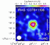
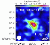
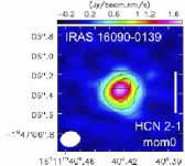
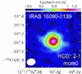
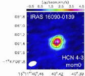
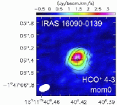
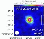
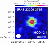
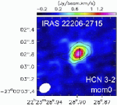
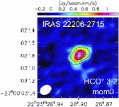
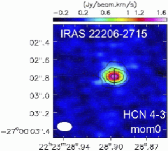
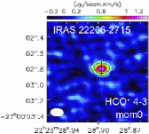
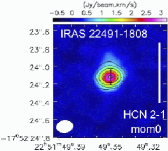
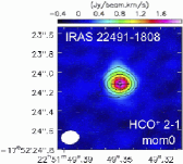
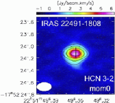
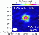
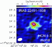
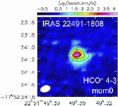
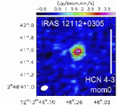
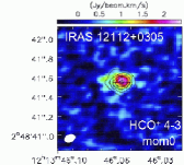
Figure 1: Integrated intensity (moment 0) map of HCN and HCO⁺ lines created from the original-beam-sized data (Table 3, column 2–4) taken in ALMA Cycle 7. Simultaneously obtained continuum emission is overplotted as contours. Continuum peak position is shown as a cross. The continuum contours start from 4$\sigma$ and increase by a factor of 2 (i.e., 8$\sigma$, 16$\sigma$, 32$\sigma$, and 64$\sigma$) for all sources. The length of the vertical white solid bar in the first image of each object corresponds to 1 kpc. Beam size for each moment 0 map is shown as a white filled circle in the lower-left region. Coordinates are in ICRS.

Table 4: Continuum Emission Properties

Object	Data	Frequency	Flux (Original beam)	Peak Coordinate	Flux (0.5 kpc)	Flux (1 kpc)
		[GHz]	[mJy/beam] (kpc$\times$kpc)	(RA,DEC)ICRS	[mJy]	[mJy]
(1)	(2)	(3)	(4)	(5)	(6)	(7)
IRAS 00091$-$0738	J21	145.3–149.0, 157.1–160.8 (153)	2.5 (98$\sigma$) (0.40$\times$0.31)	(00h11m43.3s, $-$07∘22′07′′)	2.5 (83$\sigma$)	2.7 (45$\sigma$)
(2.1 kpc/′′)	J32	236.8–241.8 (239)	5.5 (59$\sigma$) (0.39$\times$0.27)	(00h11m43.3s, $-$07∘22′07′′)	6.0 (44$\sigma$)	6.9 (24$\sigma$)
	J43	304.4–308.1, 316.4–320.1 (312)	10.7 (70$\sigma$) (0.36$\times$0.22)	(00h11m43.3s, $-$07∘22′07′′)	12.2 (46$\sigma$)	13.6 (25$\sigma$)
IRAS 00188$-$0856	J21	143.5–147.2, 155.6–159.3 (151)	0.59 (38$\sigma$) (0.49$\times$0.38)	(00h21m26.5s, $-$08∘39′26′′)	0.64 (40$\sigma$)	0.92 (32$\sigma$)
(2.3 kpc/′′)	J32	234.7–239.7 (237)	1.4 (35$\sigma$) (0.42$\times$0.29)	(00h21m26.5s, $-$08∘39′26′′)	1.8 (34$\sigma$)	2.8 (22$\sigma$)
	J43	301.6–305.3, 313.4–317.2 (309)	3.1 (40$\sigma$) (0.35$\times$0.23)	(00h21m26.5s, $-$08∘39′26′′)	4.9 (32$\sigma$)	7.8 (21$\sigma$)
IRAS 00456$-$2904	J21	146.3–150.1, 158.2–162.0 (154)	0.52 (35$\sigma$) (0.45$\times$0.33)	(00h48m06.8s, $-$28∘48′19′′)	0.63 (37$\sigma$)	0.99 (28$\sigma$)
(2.0 kpc/′′)	J32	238.5–243.4 (241)	1.2 (25$\sigma$) (0.32$\times$0.24)	(00h48m06.8s, $-$28∘48′19′′)	2.0 (24$\sigma$)	3.1 (16$\sigma$)
	J43	306.6–310.4, 318.7–322.4 (315)	2.7 (33$\sigma$) (0.38$\times$0.27)	(00h48m06.8s, $-$28∘48′19′′)	4.0 (30$\sigma$)	6.1 (19$\sigma$)
IRAS 01166$-$0844	J21	145.2–148.9, 157.2–160.9 (153)	0.35 (24$\sigma$) (0.45$\times$0.36)	(01h19m07.9s, $-$08∘29′12′′)	0.36 (25$\sigma$)	0.49 (20$\sigma$)
(2.1 kpc/′′)	J32	236.8–241.8 (239)	0.68 (17$\sigma$) (0.25$\times$0.19)	(01h19m07.9s, $-$08∘29′12′′)	1.0 (15$\sigma$)	1.5 (9.6$\sigma$)
	J43	304.6–308.4, 316.6–320.4 (313)	1.7 (28$\sigma$) (0.31$\times$0.19)	(01h19m07.9s, $-$08∘29′12′′)	2.0 (22$\sigma$)	2.6 (14$\sigma$)
IRAS 01569$-$2939	J21	142.0–145.7, 154.0–157.7 (150)	0.59 (43$\sigma$) (0.51$\times$0.36)	(01h59m13.8s, $-$29∘24′35′′)	0.62 (43$\sigma$)	0.80 (32$\sigma$)
(2.4 kpc/′′)	J32	232.2–237.2 (235)	0.70 (17$\sigma$) (0.27$\times$0.27)	(01h59m13.8s, $-$29∘24′35′′)	0.88 (16$\sigma$)	1.3 (11$\sigma$)
	J43	298.4–302.1, 310.2–313.9 (306)	1.1 (21$\sigma$) (0.52$\times$0.21)	(01h59m13.8s, $-$29∘24′35′′)	1.5 (20$\sigma$)	2.4 (17$\sigma$)
IRAS 03250$+$1606	J21	143.5–147.2, 155.6–159.2 (151)	0.35 (20$\sigma$) (0.43$\times$0.40)	(03h27m49.8s, $+$16∘16′59′′)	0.40 (23$\sigma$)	0.62 (21$\sigma$)
(2.3 kpc/′′)	J32	234.9–239.6 (237)	0.41 (14$\sigma$) (0.30$\times$0.23)	(03h27m49.8s, $+$16∘16′59′′)	0.81 (18$\sigma$)	1.5 (15$\sigma$)
	J43	301.5–305.3, 313.4–317.1 (309)	0.53 (15$\sigma$) (0.25$\times$0.19)	(03h27m49.8s, $+$16∘16′59′′)	1.6 (22$\sigma$)	3.0 (16$\sigma$)
IRAS 10378$+$1108	J21	142.4–146.2, 154.5–158.2 (150)	0.27 (13$\sigma$) (0.37$\times$0.34)	(10h40m29.2s, $+$10∘53′18′′)	0.33 (16$\sigma$)	0.53 (15$\sigma$)
(2.4 kpc/′′)	J32	233.0–238.0 (236)	1.5 (33$\sigma$) (0.40$\times$0.35)	(10h40m29.2s, $+$10∘53′18′′)	1.7 (33$\sigma$)	2.3 (21$\sigma$)
IRAS 16090$-$0139	J21	142.8–146.6, 154.9–158.6 (151)	0.51 (23$\sigma$) (0.45$\times$0.36)	(16h11m40.4s, $-$01∘47′06′′)	0.67 (29$\sigma$)	1.2 (27$\sigma$)
(2.3 kpc/′′)	J32	233.6–238.5 (236)	1.4 (20$\sigma$) (0.39$\times$0.35)	(16h11m40.4s, $-$01∘47′06′′)	1.9 (23$\sigma$)	3.5 (17$\sigma$)
	J43	300.2–303.9, 312.0–315.8 (308)	2.8 (33$\sigma$) (0.42$\times$0.24)	(16h11m40.4s, $-$01∘47′06′′)	4.8 (32$\sigma$)	7.8 (21$\sigma$)
IRAS 22206$-$2715	J21	143.0–146.7, 155.1–158.8 (151)	0.55 (38$\sigma$) (0.42$\times$0.34)	(22h23m28.9s, $-$27∘00′03′′)	0.58 (39$\sigma$)	0.73 (27$\sigma$)
(2.3 kpc/′′)	J32	233.6–239.1 (236)	1.3 (27$\sigma$) (0.42$\times$0.31)	(22h23m28.9s, $-$27∘00′03′′)	1.4 (27$\sigma$)	2.1 (18$\sigma$)
	J43	300.6–304.3, 312.4–316.2 (308)	2.8 (39$\sigma$) (0.36$\times$0.23)	(22h23m28.9s, $-$27∘00′03′′)	3.4 (32$\sigma$)	4.6 (20$\sigma$)
IRAS 22491$-$1808	J21	163.0–166.8, 175.0–178.6 (171)	1.8 (69$\sigma$) (0.24$\times$0.18)	(22h51m49.4s, $-$17∘52′24′′)	2.2 (42$\sigma$)	2.8 (24$\sigma$)
(1.5 kpc/′′)	J32	245.6–251.1 (248)	4.1 (44$\sigma$) (0.34$\times$0.18)	(22h51m49.4s, $-$17∘52′24′′)	4.9 (28$\sigma$)	5.7 (16$\sigma$)
	J43	316.2–319.7, 328.3–332.1 (324)	5.4 (48$\sigma$) (0.24$\times$0.15)	(22h51m49.4s, $-$17∘52′24′′)	8.7 (24$\sigma$)	12.3 (13$\sigma$)
IRAS 12112$+$0305	J43	317.5–321.1, 329.7–333.5 (326)	9.8 (73$\sigma$) (0.16$\times$0.10)	(12h13m46.1s, $+$02∘48′42′′)	16.7 (26$\sigma$)	20.0 (14$\sigma$)
(1.4 kpc/′′)
NGC 1614	J21	173.2–176.9, 185.4–189.1 (181)	— (0.18$\times$0.12)	(04h34m00.0s, $-$08∘34′45′′)	6.0 (11$\sigma$)	10.3 (7.5$\sigma$)
(0.32 kpc/′′)	J32	260.8–265.5 (263)	— (0.34$\times$0.19)	(04h34m00.0s, $-$08∘34′45′′)	7.3 (9.4$\sigma$)	12.5 (6.9$\sigma$)
	J43	336.1–338.1, 348.0–351.9 (344)	— (0.44$\times$0.36)	(04h34m00.0s, $-$08∘34′45′′)	14.9 (24$\sigma$)	22.1 (16$\sigma$)

Note. — Col.(1): Object name. Physical scale in kpc arcsec^-1 is shown in parentheses for reference. Col.(2): J21, J32, J43, respectively, mean continuum data simultaneously taken during J=2–1, J=3–2, and J=4–3 observations of HCN and HCO⁺. Col.(3): Frequency range in GHz used for continuum extraction is shown first. Frequencies of obvious emission and absorption lines are removed. The central frequency in GHz is shown in parenthesis. Col.(4): Flux in mJy beam^-1 at the emission peak in the original beam. Value at the highest flux pixel is extracted. The pixel scale is 0$\farcs$02 pixel^-1 for all ULIRGs’ data (This paper; Imanishi et al. (2019)). For NGC 1614 J21, J32, and J43 data, the pixel scale is 0$\farcs$05 pixel^-1, 0$\farcs$1 pixel^-1, and 0$\farcs$3 pixel^-1, respectively (Imanishi & Nakanishi, 2013a; Imanishi et al., 2016b, 2022). Detection significance relative to the root mean square (rms) noise (1$\sigma$) is shown in the first parentheses. Possible systematic uncertainties, coming from the absolute flux calibration ambiguity in individual ALMA observation and choice of frequency range for the continuum level determination, are not included. Original beam size in kpc is shown in the second parentheses. Col.(5): Coordinate of the continuum emission peak in ICRS in the original-beam-sized map. For NGC 1614, that in the 0.5 kpc beam-sized data is shown. Cols.(6) and (7): Flux in mJy at the continuum emission peak in the 0.5 kpc and 1 kpc circular beam, respectively. Detection significance relative to the rms noise (1$\sigma$) is shown in parentheses.

Table 5: Peak Flux of Molecular Emission Line in Integrated Intensity (Moment 0) Map with Original Beam Size

	Peak [Jy beam-1 km s-1]
Object	HCN J=2–1	HCO+ J=2–1	HCN J=3–2	HCO+ J=3–2	HCN J=4–3	HCO+ J=4–3	CS J=7–6	HC3N J=18–17
(1)	(2)	(3)	(4)	(5)	(6)	(7)	(8)	(9)
IRAS 00091$-$0738	1.7 (37$\sigma$)	1.3 (18$\sigma$)	2.8 (17$\sigma$)	1.5 (15$\sigma$)	3.3 (18$\sigma$)	2.2 (7.4$\sigma$)	1.6 (13$\sigma$)	0.93 (24$\sigma$)
IRAS 00188$-$0856	1.2 (33$\sigma$)	0.63 (20$\sigma$)	1.6 (25$\sigma$)	0.86 (15$\sigma$)	2.0 (20$\sigma$)	1.2 (10$\sigma$)	0.42 (7.2$\sigma$)	0.17 (7.1$\sigma$)
IRAS 00456$-$2904	0.98 (32$\sigma$)	0.63 (22$\sigma$)	1.5 (20$\sigma$)	0.76 (14$\sigma$)	2.2 (19$\sigma$)	1.3 (9.4$\sigma$)	0.31 (5.4$\sigma$)	0.15 (5.1$\sigma$)
IRAS 01166$-$0844	0.86 (22$\sigma$)	0.49 (14$\sigma$)	1.1 (16$\sigma$)	0.71 (10$\sigma$)	1.9 (16$\sigma$)	1.3 (9.1$\sigma$)	0.72 (9.1$\sigma$)	0.064 (3.1$\sigma$)
IRAS 01569$-$2939	0.85 (19$\sigma$)	0.82 (18$\sigma$)	1.1 (16$\sigma$)	1.1 (14$\sigma$)	1.7 (17$\sigma$)	1.7 (15$\sigma$)	0.55 (5.9$\sigma$)	$<$0.039 ($<$3$\sigma$)
IRAS 03250$+$1606	0.48 (11$\sigma$)	0.29 (7.6$\sigma$)	0.56 (11$\sigma$)	0.40 (8.5$\sigma$)	0.41 (8.0$\sigma$)	0.53 (5.9$\sigma$)	0.096 (3.4$\sigma$)	$<$0.066 ($<$3$\sigma$)
IRAS 10378$+$1108	0.58 (12$\sigma$)	0.54 (10$\sigma$)	1.9 (26$\sigma$)	1.8 (24$\sigma$)	—	—	—	$<$0.10 ($<$3$\sigma$)
IRAS 16090$-$0139	1.7 (26$\sigma$)	1.3 (19$\sigma$)	2.7 (26$\sigma$)	2.1 (18$\sigma$)	4.6 (25$\sigma$)	3.3 (20$\sigma$)	1.2 (12$\sigma$)	0.31 (6.7$\sigma$)
IRAS 22206$-$2715	0.91 (25$\sigma$)	0.54 (16$\sigma$)	1.5 (18$\sigma$)	1.2 (13$\sigma$)	1.6 (17$\sigma$)	1.2 (9.9$\sigma$)	0.72 (8.1$\sigma$)	0.13 (4.6$\sigma$)
IRAS 22491$-$1808	2.9 (37$\sigma$)	1.8 (26$\sigma$)	6.1 (31$\sigma$)	4.6 (23$\sigma$)	5.4 (9.5$\sigma$)	4.0 (16$\sigma$)	2.4 (16$\sigma$)	0.50 (12$\sigma$)
IRAS 12112$+$0305	—	—	—	—	3.9 (15$\sigma$)	2.3 (8.3$\sigma$)	1.2 (6.1$\sigma$)	—

Note. — Col.(1): Object name. The LIRG NGC 1614 is not shown because there are multiple emission peaks in the original-beam-sized moment 0 maps (e.g., Imanishi et al., 2016b, 2022). Cols.(2)–(9): Flux in Jy beam^-1 km s^-1 at the emission peak in the moment 0 map with the original synthesized beam (Table 3, column 2–4). Detection significance relative to the rms noise (1$\sigma$) in the moment 0 map is shown in parentheses. These original-beam-sized moment 0 maps are primarily used for the verification of significant molecular line detection at or very close to the continuum emission peak position (tabulated in Table 4, column 5). Col.(2): HCN J=2–1 (rest-frame frequency $\nu_{\rm rest}$=177.261 GHz). Col.(3): HCO⁺ J=2–1 ($\nu_{\rm rest}$=178.375 GHz). Col.(4): HCN J=3–2 ($\nu_{\rm rest}$=265.886 GHz). Col.(5): HCO⁺ J=3–2 ($\nu_{\rm rest}$=267.558 GHz). Col.(6): HCN J=4–3 ($\nu_{\rm rest}$=354.505 GHz). Col.(7): HCO⁺ J=4–3 ($\nu_{\rm rest}$=356.734 GHz). The original beam size of the J=2–1, J=3–2, and J=4–3 line is virtually identical to that of the continuum J21, J32, and J43 data shown in column 2, 3, and 4 of Table 3, respectively. Col.(8): CS J=7–6 ($\nu_{\rm rest}$=342.883 GHz). Its original beam size is comparable to that of the continuum J43 data shown in Table 3 (column 4). Col.(9): HC₃N J=18–17 ($\nu_{\rm rest}$=163.753 GHz). For IRAS 22491$-$1808, HC₃N J=21–20 ($\nu_{\rm rest}$=191.040 GHz) was covered, instead of HC₃N J=18–17. The original beam size of the HC₃N lines is comparable to that of the continuum J21 data shown in Table 3 (column 2).

To estimate nuclear dense molecular emission line (HCN and HCO⁺) fluxes from the same physical scale, we modify the original synthesized beam sizes (Table 3) to a $\sim$0.5 kpc diameter circle, using the CASA task “imsmooth” (The CASA Team, 2022) to cleaned images, for all ULIRGs, and then extract 0.5 kpc beam-sized integrated flux spectra at the continuum emission peak position. These spectra (called $\lesssim$0.5 kpc spectra) are shown in Figure 2. To investigate possible spatial variation of dense molecular line flux ratios, we also modify the original beam to 1 kpc and 2 kpc diameter circles, and extract 1 kpc and 2 kpc beam-sized integrated flux spectra (called $\lesssim$1 kpc and $\lesssim$2 kpc spectra, respectively), which are also shown in Figure 2. We also extract spectra of a 0.5–1 kpc (1–2 kpc) annular region, by subtracting the 0.5 kpc (1 kpc) beam-sized spectrum from the 1 kpc (2 kpc) beam-sized spectrum. These spectra at the 0.5–1 kpc and 1–2 kpc annular regions (named 0.5–1 kpc and 1–2 kpc spectra, respectively) are shown in Figure 3, by overplotting on the $\lesssim$0.5 kpc spectra. In making these new fixed-physical-scale spectra, we need to note that in interferometric data, when we modify the originally very small beam size to a large beam size, the resulting rms noise in units of mJy beam^-1 increases. The resulting large-beam-sized spectrum can become noisy with large scatters. In fact, the scatters of data points are generally larger for the 1–2 kpc and $\lesssim$2 kpc spectra than the 0.5–1 kpc and $\lesssim$0.5 kpc spectra (Figures 2 and 3), because we enlarge the originally small beam size ($\lesssim$0.5 kpc) to 2 kpc. Thus, unless molecular emission line flux increases substantially, its detection significance decreases in the large-beam-sized spectra. For the observed ULIRGs, HCN and HCO⁺ emission line signals in the 1–2 kpc spectra are generally not large, even fainter than those in the $\lesssim$0.5 kpc spectra (Figure 3), despite the fact that the signal-integrated area of the 1–2 kpc annular region is a factor of 12 larger than that of the central 0.5 kpc circular region. This is as expected because the bulk of dense molecular gas in nearby ULIRGs’ nuclei is usually concentrated into the central compact ($\lesssim$1 kpc) regions (e.g., Imanishi et al., 2018, 2022). Thus, we can obtain meaningful estimates of HCN and HCO⁺ emission line fluxes at the 1–2 kpc annular region only for a limited fraction of the observed ULIRGs.

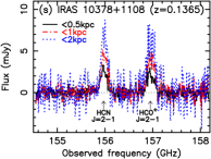
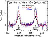
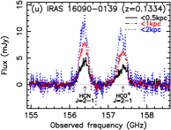
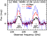
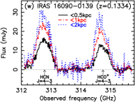
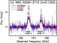
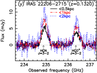
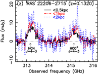
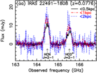
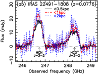
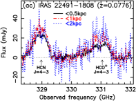
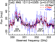
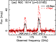
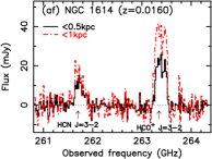
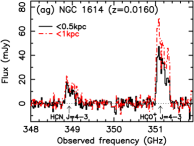
Figure 2: Spectra within central 0.5 kpc (black solid line), 1 kpc (red dash-dotted line), and 2 kpc (blue dotted line) regions. The abscissa is observed frequency in GHz and the ordinate is flux density in mJy. (Left): J=2–1 of HCN and HCO⁺. (Middle): J=3–2 of HCN and HCO⁺. (Right): J=4–3 of HCN and HCO⁺. The expected frequency of HCN and HCO⁺ J=2–1, J=3–2, and J=4–3 lines, at the adopted redshift of each (U)LIRG (column 2 of Table 1; also displayed at the top of each plot), is indicated with vertical arrow. The horizontal black thin dotted straight line indicates the zero flux level. For the LIRG NGC 1614, $\lesssim$2 kpc spectra are not extracted because no meaningful information of molecular line emission at $\gtrsim$1 kpc is obtained from our ALMA data.

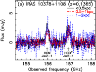
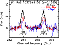
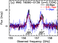
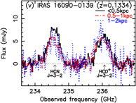
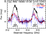
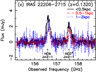
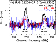
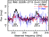
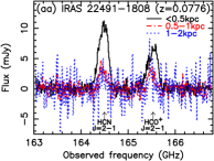
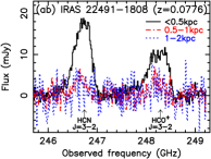
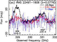
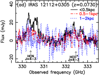
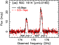
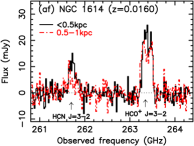
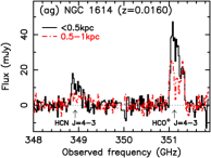
Figure 3: Spectra within central 0.5 kpc (black solid line), 0.5–1 kpc annular (red dash-dotted line), and 1–2 kpc annular (blue dotted line) regions, displayed in the same way as Figure 2. The 1–2 kpc spectra of the LIRG NGC 1614 are not shown for the same reason as explained in Figure 2 caption.

Gaussian fits are applied to significantly detected HCN and HCO⁺ emission lines in the spectra at various regions. Following Imanishi et al. (2023), to simplify our flux estimates, we try to apply a single Gaussian fit, as long as a line profile can be approximated by a single emission component. We apply a double Gaussian fit only if an emission line displays a clear double-peaked profile with a deep central dip. Our final adopted best Gaussian fits are summarized in Appendix C. Table 6 tabulates the derived Gaussian-fit velocity-integrated emission line fluxes of HCN and HCO⁺.

Figure 4 shows the curve of growth of HCN and HCO⁺ emission line fluxes at J=2–1, J=3–2, and J=4–3, with increasing beam size from 0.5 kpc, through 1 kpc, to 2 kpc. We see that in the majority of the observed ULIRGs, HCO⁺ flux increases more significantly than HCN flux when compared at the same J-transition, supporting a previous suggestion that HCO⁺ emission is spatially more extended than HCN emission in nearby ULIRGs’ nuclei (Imanishi et al., 2019). This is reasonable because the factor of $\sim$5 smaller critical density of HCO⁺ than that of HCN at the same J-transition (Shirley, 2015) can make HCO⁺ excitation more efficient than HCN at the outer nuclear (0.5–2 kpc) region where molecular gas density and temperature are likely to be smaller than those at the innermost ($\lesssim$0.5 kpc) region. It is also found that the flux increase with increasing aperture size tends to be smaller at J=4–3 than at J=2–1, which can also be explained if gas density and temperature at the outer nuclear (0.5–2 kpc) region are not very high to sufficiently excite HCN and HCO⁺ to J=4.

The CS J=7–6 ($\nu_{\rm rest}$ = 342.883 GHz) emission line was also clearly detected in all ULIRGs during HCN and HCO⁺ J=4–3 line observations. Appendix D summarizes the original-beam-sized moment 0 map, 0.5 kpc beam-sized spectrum, and Gaussian fit in the spectrum, for the CS J=7–6 line.

HC₃N J=18–17 ($\nu_{\rm rest}$ = 163.753 GHz) or J=21–20 ($\nu_{\rm rest}$ = 191.040 GHz) emission line was also serendipitously detected during the HCN and HCO⁺ J=2–1 line observations of all ULIRGs. Appendix E summarizes the original-beam-sized moment 0 map, 0.5 kpc beam-sized spectrum, and Gaussian fit in the spectrum, for the HC₃N lines. The peak fluxes of the CS J=7–6 and HC₃N emission lines in the original-beam-sized moment 0 maps are also added in columns 8 and 9 of Table 5, respectively.

We summarize in Appendix F (i) the observed HCN-to-HCO⁺ flux ratios at J=2–1, J=3–2, and J=4–3, and (ii) the observed high-J to low-J flux ratios of HCN and HCO⁺, based on the adopted Gaussian fits (Appendix C), in the $\lesssim$0.5 kpc, $\lesssim$1 kpc, $\lesssim$2 kpc, 0.5–1 kpc, and 1–2 kpc spectra. These ratios are plotted in Figures 5 and 6, respectively, to visualize how the ratios vary in different regions.

Table 6: Gaussian-fit Velocity-integrated Flux of HCN and HCO⁺ Emission Lines

Object	Region	Flux (Jy km s-1)
		HCN			HCO+
		J=2–1	J=3–2	J=4–3	J=2–1	J=3–2	J=4–3
(1)	(2)	(3)	(4)	(5)	(6)	(7)	(8)
IRAS 00091$-$0738	$\lesssim$0.5 kpc	2.1$\pm$0.1	4.0$\pm$0.8	4.9$\pm$0.4	1.6$\pm$0.2	2.1$\pm$0.7	3.5$\pm$1.0
	$\lesssim$1 kpc	2.4$\pm$0.2	5.5$\pm$1.2	6.3$\pm$0.9	2.2$\pm$0.3	3.0$\pm$1.1	5.0$\pm$1.1
	$\lesssim$2 kpc	2.7$\pm$0.4	6.5$\pm$1.3	6.8$\pm$1.7	2.7$\pm$0.6	4.1$\pm$0.7	7.7$\pm$2.5
	0.5–1 kpc	0.30$\pm$0.07	1.4$\pm$0.4	1.7$\pm$1.4	0.49$\pm$0.16	0.94$\pm$0.27	0.53$\pm$0.34
	1–2 kpc	0.30$\pm$0.16	1.1$\pm$0.3	—	0.49$\pm$0.36	1.3$\pm$0.5	—
IRAS 00188$-$0856	$\lesssim$0.5 kpc	1.5$\pm$0.1	2.4$\pm$0.1	3.6$\pm$0.2	0.83$\pm$0.05	1.4$\pm$0.1	1.9$\pm$0.4
	$\lesssim$1 kpc	2.2$\pm$0.1	4.0$\pm$0.1	5.2$\pm$0.9	1.4$\pm$0.1	2.4$\pm$0.1	2.5$\pm$0.5
	$\lesssim$2 kpc	2.9$\pm$0.1	5.4$\pm$0.3	7.3$\pm$0.6	1.8$\pm$0.1	3.1$\pm$0.2	2.8$\pm$0.7
	0.5–1 kpc	0.71$\pm$0.05	1.5$\pm$0.1	1.6$\pm$0.4	0.53$\pm$0.06	0.98$\pm$0.09	0.63$\pm$0.20
	1–2 kpc	0.63$\pm$0.09	1.4$\pm$0.2	1.9$\pm$0.6	0.48$\pm$0.16	0.69$\pm$0.17	—
IRAS 00456$-$2904	$\lesssim$0.5 kpc	1.3$\pm$0.1	2.9$\pm$0.1	3.6$\pm$0.2	0.91$\pm$0.05	1.6$\pm$0.1	2.2$\pm$0.2
	$\lesssim$1 kpc	2.1$\pm$0.1	4.3$\pm$0.3	5.2$\pm$0.3	1.5$\pm$0.1	2.8$\pm$0.2	3.0$\pm$0.4
	$\lesssim$2 kpc	2.7$\pm$0.1	5.2$\pm$0.4	6.3$\pm$0.6	2.0$\pm$0.1	4.1$\pm$0.5	3.7$\pm$0.7
	0.5–1 kpc	0.72$\pm$0.05	1.4$\pm$0.2	1.4$\pm$0.4	0.56$\pm$0.06	1.2$\pm$0.2	0.79$\pm$0.24
	1–2 kpc	0.67$\pm$0.10	0.88$\pm$0.29	1.2$\pm$0.5	0.56$\pm$0.12	1.3$\pm$0.4	0.88$\pm$0.41
IRAS 01166$-$0844	$\lesssim$0.5 kpc	1.2$\pm$0.1	1.8$\pm$0.2	2.8$\pm$0.2	0.64$\pm$0.07	1.4$\pm$0.2	1.8$\pm$0.2
	$\lesssim$1 kpc	1.4$\pm$0.1	3.0$\pm$0.5	3.1$\pm$0.3	0.84$\pm$0.09	2.2$\pm$0.3	2.2$\pm$0.3
	$\lesssim$2 kpc	1.7$\pm$0.2	4.0$\pm$0.9	3.2$\pm$0.8	1.2$\pm$0.2	2.4$\pm$0.6	2.3$\pm$0.7
	0.5–1 kpc	0.21$\pm$0.06	1.2$\pm$0.4	0.35$\pm$0.51	0.20$\pm$0.07	0.81$\pm$0.20	0.37$\pm$0.28
	1–2 kpc	0.21$\pm$0.14	—	—	0.45$\pm$0.40	—	—
IRAS 01569$-$2939	$\lesssim$0.5 kpc	1.0$\pm$0.1	1.8$\pm$0.2	2.3$\pm$0.2	1.0$\pm$0.2	2.1$\pm$0.3	2.5$\pm$0.3
	$\lesssim$1 kpc	1.3$\pm$0.2	2.8$\pm$0.7	3.2$\pm$0.3	1.5$\pm$0.2	3.7$\pm$0.3	3.4$\pm$0.5
	$\lesssim$2 kpc	1.8$\pm$0.2	3.8$\pm$0.5	3.8$\pm$0.7	1.9$\pm$0.2	4.8$\pm$0.5	4.3$\pm$0.8
	0.5–1 kpc	0.29$\pm$0.08	1.0$\pm$0.2	0.87$\pm$0.16	0.40$\pm$0.09	1.5$\pm$0.2	0.82$\pm$0.21
	1–2 kpc	0.43$\pm$0.22	0.84$\pm$0.34	0.67$\pm$0.26	0.40$\pm$0.13	1.1$\pm$0.35	0.94$\pm$0.54
IRAS 03250$+$1606	$\lesssim$0.5 kpc	0.67$\pm$0.07	1.3$\pm$0.2	1.2$\pm$0.2	0.47$\pm$0.08	0.92$\pm$0.22	0.97$\pm$0.30
	$\lesssim$1 kpc	1.1$\pm$0.1	2.0$\pm$0.4	2.0$\pm$0.6	0.92$\pm$0.12	1.7$\pm$0.4	1.6$\pm$0.4
	$\lesssim$2 kpc	1.3$\pm$0.2	2.7$\pm$0.4	2.4$\pm$0.6	1.5$\pm$0.3	2.6$\pm$0.3	2.3$\pm$0.9
	0.5–1 kpc	0.39$\pm$0.08	0.71$\pm$0.17	0.86$\pm$0.17	0.44$\pm$0.12	0.80$\pm$0.23	0.66$\pm$0.23
	1–2 kpc	0.28$\pm$0.13	0.70$\pm$0.33	—	0.61$\pm$0.25	0.85$\pm$0.21	0.56$\pm$0.36
IRAS 10378$+$1108	$\lesssim$0.5 kpc	0.90$\pm$0.08	2.7$\pm$0.1	—	0.82$\pm$0.09	2.5$\pm$0.1	—
	$\lesssim$1 kpc	1.5$\pm$0.1	4.1$\pm$0.2	—	1.6$\pm$0.1	3.8$\pm$0.2	—
	$\lesssim$2 kpc	2.2$\pm$0.2	5.2$\pm$0.4	—	2.6$\pm$0.3	5.0$\pm$0.4	—
	0.5–1 kpc	0.56$\pm$0.09	1.3$\pm$0.1	—	0.72$\pm$0.13	1.4$\pm$0.1	—
	1–2 kpc	0.73$\pm$0.18	1.2$\pm$0.2	—	1.1$\pm$0.3	1.1$\pm$0.3	—
IRAS 16090$-$0139	$\lesssim$0.5 kpc	2.4$\pm$0.1	4.1$\pm$0.2	8.3$\pm$0.2	1.9$\pm$0.1	3.3$\pm$0.2	5.8$\pm$0.2
	$\lesssim$1 kpc	4.0$\pm$0.1	6.9$\pm$0.3	12.6$\pm$0.4	3.4$\pm$0.1	6.5$\pm$0.4	9.4$\pm$0.5
	$\lesssim$2 kpc	5.3$\pm$0.2	9.5$\pm$0.6	15.5$\pm$0.7	5.0$\pm$0.3	10.3$\pm$0.7	12.1$\pm$0.6
	0.5–1 kpc	1.6$\pm$0.1	2.8$\pm$0.2	4.3$\pm$0.3	1.5$\pm$0.1	3.2$\pm$0.2	3.6$\pm$0.2
	1–2 kpc	1.4$\pm$0.2	2.5$\pm$0.4	2.9$\pm$0.6	1.5$\pm$0.2	3.7$\pm$0.5	2.5$\pm$0.4
IRAS 22206$-$2715	$\lesssim$0.5 kpc	1.3$\pm$0.1	2.1$\pm$0.1	2.8$\pm$0.2	0.86$\pm$0.08	1.5$\pm$0.1	2.2$\pm$0.2
	$\lesssim$1 kpc	1.8$\pm$0.1	3.0$\pm$0.2	4.0$\pm$0.3	1.2$\pm$0.1	2.2$\pm$0.2	2.8$\pm$0.3
	$\lesssim$2 kpc	2.4$\pm$0.2	4.1$\pm$0.3	5.0$\pm$0.7	1.3$\pm$0.2	2.7$\pm$0.3	4.3$\pm$0.9
	0.5–1 kpc	0.51$\pm$0.05	0.99$\pm$0.14	1.1$\pm$0.2	0.35$\pm$0.08	0.61$\pm$0.11	0.63$\pm$0.21
	1–2 kpc	0.58$\pm$0.13	1.2$\pm$0.4	1.1$\pm$0.6	0.23$\pm$0.11	0.48$\pm$0.23	1.6$\pm$0.8
IRAS 22491$-$1808	$\lesssim$0.5 kpc	4.8$\pm$0.1	9.2$\pm$0.3	12.4$\pm$0.4	3.2$\pm$0.1	6.4$\pm$0.3	8.3$\pm$0.6
	$\lesssim$1 kpc	5.9$\pm$0.2	10.7$\pm$0.4	15.7$\pm$0.9	4.1$\pm$0.2	7.4$\pm$0.5	13.1$\pm$1.3
	$\lesssim$2 kpc	6.2$\pm$0.5	11.8$\pm$0.9	14.7$\pm$2.0	4.6$\pm$0.5	8.4$\pm$0.9	16.1$\pm$3.1
	0.5–1 kpc	1.1$\pm$0.2	1.6$\pm$0.3	3.3$\pm$0.7	0.95$\pm$0.16	1.2$\pm$0.3	4.2$\pm$0.9
	1–2 kpc	0.50$\pm$0.33	—	—	0.56$\pm$0.22	—	—
IRAS 12112$+$0305	$\lesssim$0.5 kpc	—	—	11.6$\pm$1.2	—	—	6.7$\pm$1.0
	$\lesssim$1 kpc	—	—	18.4$\pm$1.6	—	—	11.3$\pm$1.8
	$\lesssim$2 kpc	—	—	19.6$\pm$3.6	—	—	13.0$\pm$3.3
	0.5–1 kpc	—	—	5.5$\pm$1.6	—	—	2.8$\pm$1.9
	1–2 kpc	—	—	—	—	—	—
NGC 1614	$\lesssim$0.5 kpc	3.3$\pm$0.2	2.6$\pm$0.4	2.6$\pm$0.4	5.5$\pm$0.2	5.9$\pm$0.5	8.5$\pm$0.7
	$\lesssim$1 kpc	6.8$\pm$0.4	4.2$\pm$0.8	4.3$\pm$0.5	12.3$\pm$0.5	11.3$\pm$0.9	13.9$\pm$1.2
	0.5–1 kpc	3.5$\pm$0.3	1.6$\pm$0.7	2.0$\pm$0.5	6.8$\pm$0.3	5.4$\pm$0.7	5.3$\pm$1.0

Note. — Col.(1): Object name. Col.(2): Region. Central $\lesssim$0.5 kpc, $\lesssim$1 kpc, $\lesssim$2 kpc, 0.5–1 kpc annular, and 1–2 kpc annular regions. Cols.(3)–(8): Gaussian-fit velocity-integrated flux in units of Jy km s^-1 (Appendix C). Col.(3): HCN J=2–1. Col.(4): HCN J=3–2. Col.(5): HCN J=4–3. Col.(6): HCO⁺ J=2–1. Col.(7): HCO⁺ J=3–2. Col.(8): HCO⁺ J=4–3. No value is shown when (a) no observations were conducted (J=4–3 of IRAS 10378$+$1108, and J=2–1 and J=3–2 of IRAS 12112$+$0305), or (b) there is no emission line signature at all, or (c) fitting uncertainty is too large to obtain meaningful information.

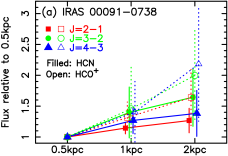
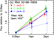
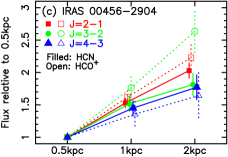
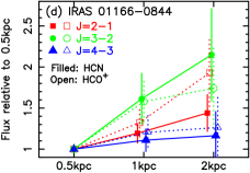
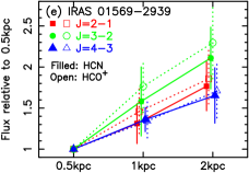
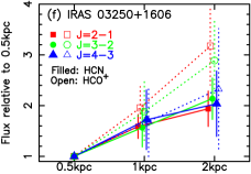
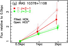
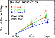
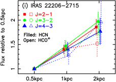
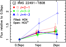
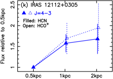
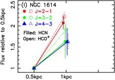
Figure 4: Curve of growth of HCN (filled symbol) and HCO⁺ (open symbol) emission line flux, based on our adopted Gaussian fit (Appendix C), with increasing beam size from 0.5 kpc, through 1 kpc, to 2 kpc. Red square: J=2–1. Green circle: J=3–2. Blue triangle: J=4–3.

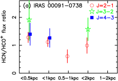
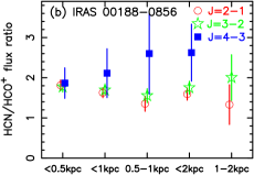
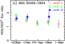
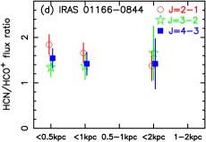
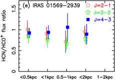
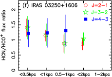
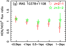
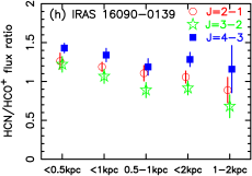
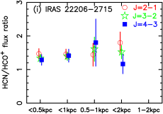
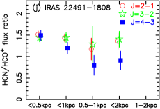
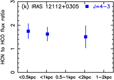
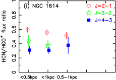
Figure 5: HCN-to-HCO⁺ flux ratio measured in the $\lesssim$0.5 kpc, $\lesssim$1 kpc, 0.5–1 kpc, $\lesssim$2 kpc, and 1–2 kpc spectra. Red open circle: J=2–1. Green open star: J=3–2. Blue filled square: J=4–3. Only ratios with $\gtrsim$2.5$\sigma$ are plotted. Note that the vertical axis range of the only one LIRG NGC 1614 is much narrower than ULIRGs.

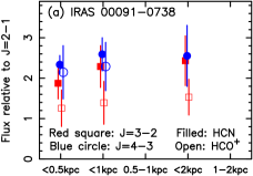
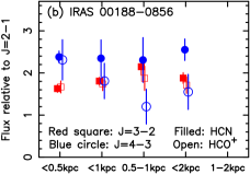
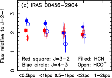
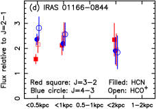
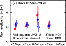
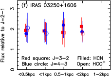
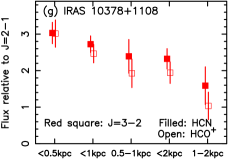
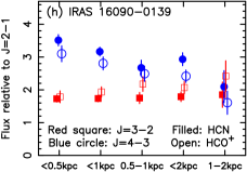
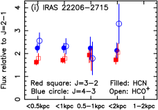
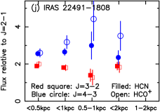
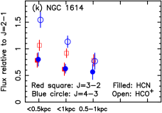
Figure 6: J=4–3 (blue circle) or J=3–2 (red square) to J=2–1 flux ratio of HCN (filled symbol) and HCO⁺ (open symbol), measured in the $\lesssim$0.5 kpc, $\lesssim$1 kpc, 0.5–1 kpc, $\lesssim$2 kpc, and 1–2 kpc spectra. Only Gaussian fit statistical uncertainty is considered, and only ratios with $\gtrsim$2.5$\sigma$ are plotted. The vertical axis range of the only one LIRG NGC 1614 is much narrower than ULIRGs.

In each panel of Figure 5, in the left three ticks, the contribution from the innermost ($\lesssim$0.5 kpc) molecular gas emission, relative to slightly extended (0.5–1 kpc) emission, decreases from left to right. In the right two ticks, the contribution from the outermost nuclear (1–2 kpc) molecular gas emission, relative to inner ($\lesssim$1 kpc) emission, increases from left to right. In many sources, we see a subtle trend that the observed HCN-to-HCO⁺ flux ratio at each J-transition slightly decreases with decreasing contribution from the innermost ($\lesssim$0.5 kpc) molecular emission (from left to right in the left three ticks) and with increasing contribution from the outermost nuclear (1–2 kpc) emission (from left to right in the right two ticks). This trend is most notably seen in IRAS 16090$-$0139 (Figure 5h), because of small uncertainty in each data point. It is thus suggested that the HCN-to-HCO⁺ flux ratio is higher inside and lower outside in a certain fraction of nearby ULIRGs’ nuclei. Figure 7 displays the original-beam-sized maps of the observed HCN-to-HCO⁺ flux ratios at J=2–1, J=3–2, and J=4–3, created from newly taken ALMA Cycle 7 data (Table 3). The same maps at J=3–2 for some ULIRGs, created from ALMA Cycle 5 data (Table 3), are also found in Imanishi et al. (2019). In some ULIRGs, the HCN-to-HCO⁺ flux ratio is confirmed to be higher at the very center (nuclear position) than off-center regions (e.g., IRAS 16090$-$0139).

We see a similar trend in some ULIRGs in Figure 6 that the observed high-J to low-J flux ratio slightly decreases with decreasing (increasing) contribution from $\lesssim$0.5 kpc (1–2 kpc) molecular emission, where the trend is most clearly seen in the J=3–2 to J=2–1 flux ratios of HCN and HCO⁺ in IRAS 10378$+$1108 (Figure 6g) and J=4–3 to J=2–1 flux ratios of HCN and HCO⁺ in IRAS 16090$-$0139 (Figure 6h). These decreasing trends from the innermost to outermost nuclear region, in the HCN-to-HCO⁺ flux ratio and high-J to low-J flux ratios of HCN and HCO⁺, suggest that possible spatial variation of dense molecular gas properties is discernible at 0.5 kpc physical scales within the nuclear 2 kpc regions of some ULIRGs.

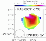
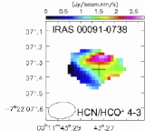
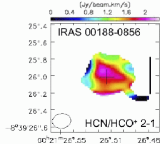
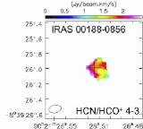
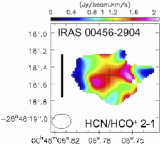
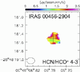
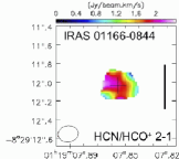
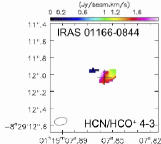
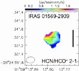
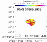
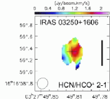
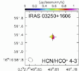
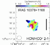
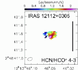
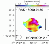
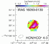
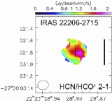
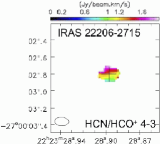
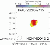
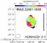
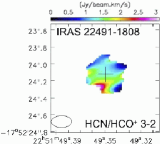
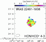
Figure 7: Original-beam-sized map of the observed HCN-to-HCO⁺ flux ratio calculated in units of Jy km s^-1. An appropriate cutoff ($>$2–3$\sigma$ depending on each ULIRG) is applied for the HCO⁺ flux (i.e., denominator), so that the resulting map is not dominated by noise. The plus mark denotes the continuum peak position which is regarded as the nucleus of each ULIRG. The length of the vertical black solid bar in the first image of each object corresponds to 1 kpc.

In Figure 8, we derive the HCN J=4–3 to HCO⁺ J=4–3 and HCN J=4–3 to CS J=7–6 flux ratios measured in the $\lesssim$0.5 kpc spectra, to separate AGN-important and starburst-dominated sources, following the energy diagnostic diagram by Izumi et al. (2016) where these flux ratios are systematically higher in luminous AGNs than in starbursts. The LIRG NGC 1614 is located in the region expected for starburst-dominated galaxies, while ULIRGs (except IRAS 01569$-$2939) are distributed in the region expected for AGN-important galaxies. The ULIRG IRAS 01569$-$2939 is located close to the borderline that separates starburst-dominated and AGN-important galaxies. The energy diagnostic results in Figure 8 thus largely agree with the previously proposed infrared and (sub)millimeter spectroscopic view that all ULIRGs are AGN important and the LIRG NGC 1614 is starburst dominated (Table 1, column 12 and footnote a).

Figure 8: HCN J=4–3 to HCO⁺ J=4–3 flux ratio (abscissa) and HCN J=4–3 to CS J=7–6 flux ratio (ordinate) derived from the 0.5 kpc beam-sized spectra. Flux ratio is calculated in units of Jy km s^-1. Izumi et al. (2016) proposed that starburst-dominated galaxies are distributed in the lower-left region separated by the dashed straight lines, while AGN-important galaxies are in the remaining upper-right region.

5 Discussion

5.1 Dense Molecular Gas Properties : Comparison with Non-LTE Model Calculations

We constrain nuclear molecular gas properties of the observed (U)LIRGs at 0.5 kpc physical resolution, based on the three J-transition line data (J=2–1, J=3–2, and J=4–3) of HCN and HCO⁺, by combining with non-LTE modeling. The high-J to low-J flux ratios of HCN and HCO⁺ can be used to constrain the volume number density (n${}_{\rm H_{2}}$) and kinetic temperature (T_kin) of H₂ molecular gas, because high density and temperature are needed to collisionally excite a significant fraction of HCN and HCO⁺ to J=4 or 3. The HCN-to-HCO⁺ flux ratio at each J-transition contains information of the HCN-to-HCO⁺ abundance ratio, as was demonstrated by Imanishi et al. (2023) for other nearby (U)LIRGs. The possible decrease of the HCN-to-HCO⁺ flux ratio from low-J to high-J can also contain H₂ gas density information (e.g., Imanishi et al., 2023); Because the critical density of HCN by H₂ collisional excitation is a factor of $\sim$5 higher than that of HCO⁺ at each J-transition (Shirley, 2015), the HCN-to-HCO⁺ flux ratio can be smaller at higher-J than at lower-J if H₂ gas density is not sufficiently high.

To derive molecular gas properties, we compare observed emission line flux ratios with those calculated with the non-LTE radiative transfer code RADEX (van der Tak et al., 2007), as we have done for other nearby (U)LIRGs’ nuclei using 1–2 kpc resolution data (Imanishi et al., 2023). Here, we do the same comparison for the newly observed nearby ULIRGs’ nuclei (Table 1). We also investigate the possible spatial variation of molecular gas properties within the nuclear $\lesssim$2 kpc regions, using our 0.5 kpc resolution data. For all RADEX calculations, (1) gas geometry is assumed to be a one-zone uniform sphere, (2) the cosmic microwave background with temperature of T_bg = 2.73 K is included, and (3) collisions with only H₂ are considered. The molecular line width is commonly set to 500 km s^-1 as a representative value, based on our Gaussian fits (Appendix C). Emission line flux ratios are calculated in units of Jy km s^-1 as listed in Tables 12 and 13 in Appendix C. For convenience, pyradex, a Python wrapper for RADEX, is used.

In our model calculations, we adopt two approaches, following Imanishi et al. (2023). First, we constrain molecular gas density and temperature, by fixing the HCN-to-HCO⁺ abundance ratio and HCO⁺ column density to fiducial values ($\S$5.2–5.3), because the number of observational constraints is limited. Next, we apply a Bayesian approach to constrain physical parameters, by making all parameters free ($\S$5.4), with a caution that some parameters may have systematic uncertainties, given so many free parameters for the limited number of observational constrains. We will then compare both results to confirm that our main arguments do not change and thus are robust.

5.2 HCN-to-HCO⁺ Flux Ratios

Figure 9 compares the HCN-to-HCO⁺ flux ratios at J=2–1, J=3–2, and J=4–3 measured in the 0.5 kpc beam-sized spectra, with predicted flux ratios by RADEX; RADEX calculations are made at densities 10^3-8 cm^-3 and temperatures 10^1-3 K. The HCO⁺ column density is fixed at N_HCO+ = 1 $\times$ 10¹⁶ cm^-2, based on the assumption that the observed (U)LIRGs suffer from modestly Compton thick (N_H $\sim$ a few $\times$ 10²⁴ cm^-2) absorption and the HCO⁺-to-H₂ abundance ratio is $\sim$10^-8 (e.g., Martin et al., 2006; Saito et al., 2018). The HCN-to-HCO⁺ abundance ratio is tested for two cases, [HCN]/[HCO⁺] = 1 and 3.

Except for the LIRG NGC 1614 (the most bottom-left red filled star in Figure 9), the observed HCN-to-HCO⁺ flux ratios of all ULIRGs can be better explained by the HCN-to-HCO⁺ abundance ratio of [HCN]/[HCO⁺] = 3 rather than 1, under the above assumed gas density and temperature ranges. We also try different HCN-to-HCO⁺ abundance ratio ([HCN]/[HCO⁺] = 7) and HCO⁺ column density (N_HCO+ = 1 $\times$ 10¹⁵ cm^-2 and 3 $\times$ 10¹⁶ cm^-2), but our conclusion that the observed HCN-to-HCO⁺ flux ratios of ULIRGs are better reproduced with an enhanced ($>$1) HCN-to-HCO⁺ abundance ratio, remains unchanged (Appendix G), as previously confirmed for other nearby ULIRGs, calculated with different line widths (Imanishi et al., 2023). We conservatively adopt [HCN]/[HCO⁺] = 3 as a fiducial value.

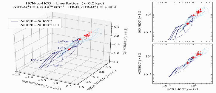
Figure 9: Comparison of the HCN-to-HCO⁺ flux ratios measured in the 0.5 kpc beam-sized spectra and those calculated with RADEX. (Left panel): 3D plot of the flux ratios at J=2–1, J=3–2, and J=4–3. The red points represent the observed values. The RADEX-calculated flux ratios are computed for log n${}_{\rm H_{2}}$/cm^-3 = 3–8 in steps of 0.1 (density) and log (T_kin/K) = 1–3 in steps of 0.05 (temperature). The ratios are shown as a blue mesh consisting of iso-density curves at log n${}_{\rm H_{2}}$ = 3, 4, $\cdots$, 8 (solid), and iso-temperature curves at log T_kin = 1.0, 1.5, $\cdots$, 3.0 (dotted). The molecular line width and HCO⁺ column density are fixed at $\Delta$v = 500 km s^-1 and N_HCO+ = 1 $\times$ 10¹⁶ cm^-2, respectively. The results of the HCN-to-HCO⁺ abundance ratio of [HCN]/[HCO⁺] = 1 and 3 are drawn in dark and light colors, respectively. (Right panels): Projections of the 3D plot along the J=3–2 (upper) and J=4–3 (lower) directions.

5.3 High-J to Low-J Flux Ratios

We fit the observed high-J to low-J flux ratios of HCN and HCO⁺ with RADEX to estimate molecular gas density and temperature. The method is the same as that employed by Imanishi et al. (2023). The least-squares fitting for log n${}_{\rm H_{2}}$ (density) and log T_kin (temperature) is performed with the conventional Levenberg-Marquardt algorithm using the Python package lmfit (Newville et al., 2021). Confidence intervals for the parameters are examined by grid computing $\Delta\chi^{2}\equiv\chi^{2}-\chi^{2}_{\rm best}$ with log n${}_{\rm H_{2}}$ ranging from 2 to 6 and log T_kin from 1 to 3.

As described by Imanishi et al. (2023) and in $\S$3, the high-J to low-J flux ratios of HCN and HCO⁺ can be affected by possible absolute flux calibration uncertainty of individual ALMA observations, because J=2–1, J=3–2, and J=4–3 data were taken at different times. This systematic uncertainty needs to be taken into account when we compare the observed and RADEX-calculated flux ratios. As our second calculations, we allow scaling of absolute flux within maximum 5$\%$ for J=2–1 and 10$\%$ for J=3–2 and J=4–3 ($\S$3). We divide the fitting into two stages: in the first stage, gas density, temperature, and scaling of each emission line flux within the calibration uncertainty are left free, and the residuals are minimized using the L-BFGS-B method; in the second stage, the scaling factors are fixed to the obtained values. We then derive gas density and temperature using the Levenberg-Marquardt algorithm with the Python package lmfit (Newville et al., 2021), in the same way as above.

We derive molecular gas physical parameters, by (1) using the observed high-J to low-J flux ratios as they are (no flux scaling), and (2) allowing flux scale adjustment for individual J=2–1, J=3–2, and J=4–3 data within the above allowable range (5–10$\%$). The derived gas density and temperature are generally comparable between the first and second methods, but the reduced $\chi^{2}$ value is usually smaller in the second fitting result (scaling on) than the first one (scaling off). We adopt the first one as much as possible, but refer to the second one only if the first one cannot determine the best fit value or provides a very large reduced $\chi^{2}$ value. Our adopted final results for the central $\lesssim$0.5 kpc region are presented in Figures 10 and 11a, and are summarized in Table 7. The same results for the central $\lesssim$1 kpc and $\lesssim$2 kpc regions are presented in Appendix H, to be compared with those derived for different nearby ULIRGs with comparable 1–2 kpc resolutions by Imanishi et al. (2023). We exclude IRAS 10378$+$1108 and IRAS 12112$+$0305 because not all the three J-transition line data are available. We exclude also IRAS 00091$-$0738 because negative signals below the continuum levels, clearly detected at the HCO⁺ central absorption dips in Figures 2 and 3, suggest self-absorption (see also Appendix C, Table 9, footnote a). Namely, molecular gas consists of more than one component (i.e., emission and absorption components), which complicates comparison between the observed data and one-zone RADEX model calculations.

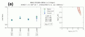
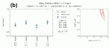
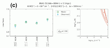
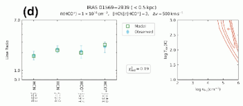
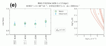
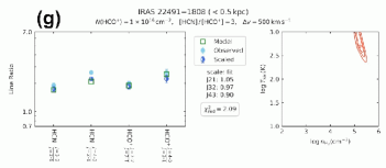
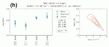
Figure 10: Fitting results for the high-J to low-J flux ratios of HCN and HCO⁺ for the central $\lesssim$0.5 kpc regions of (U)LIRGs. (Left panel): Comparison of the observed and RADEX-calculated emission line flux ratios. The light blue filled circles show the observed flux ratios listed in Table 13. The green open squares indicate the flux ratios of the best-fit model, whose gas density and temperature are denoted as the plus sign in the right panel. Other fixed parameters (column density, abundance ratio, and line width) are noted at the top of the figure. We adopt the second fitting results (flux scaling adjustment allowed; see $\S$5.3) for IRAS 00188$-$0856, IRAS 00456$-$2904, IRAS 22491$-$1808, and NGC 1614, for which the observed flux ratios after scaling adjustment are displayed in the dark blue half-filled circles. The scaling factors for each observation are listed below the legend. The reduced $\chi^{2}$ value of the best-fit model is also noted. (Right panel): Confidence contours for gas density and temperature quoted at 68%, 90%, and 99% levels ($\Delta\chi^{2}=2.28,4.61,9.21$). Result of IRAS 16090$-$0139 is displayed separately in Figure 11a.

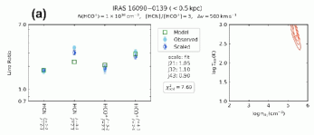
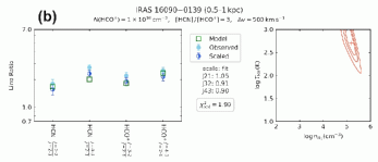
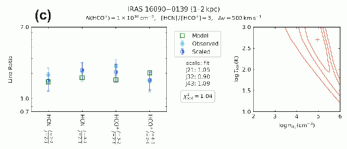
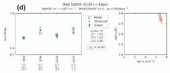
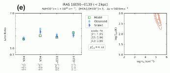
Figure 11: Fitting results for the high-J to low-J flux ratios of HCN and HCO⁺ for various regions of IRAS 16090$-$0139. (a): central $\lesssim$0.5 kpc region. (b): 0.5–1 kpc annular region. (c): 1–2 kpc annular region. (d): central $\lesssim$1 kpc region. (e): central $\lesssim$2 kpc region. We adopt the second fitting result (flux scaling adjustment allowed) for all regions. The content of each panel and symbols are the same as Figure 10.

Table 7: Summary of the Best Fit Values

Object	Region	Scaling	log n${}_{\rm H_{2}}$	log Tkin	Reduced
			[cm-3]	[K]	$\chi^{2}$
(1)	(2)	(3)	(4)	(5)	(6)
IRAS 00188$-$0856	$<$0.5 kpc	on	5.2${}^{+0.1}_{-0.2}$	2.7${}^{+0.6}_{-0.1}$	0.50
IRAS 00456$-$2904	$<$0.5 kpc	on	5.2${}^{+0.1}_{-0.2}$	2.7${}^{+0.3}_{-0.1}$	3.3
IRAS 01166$-$0844	$<$0.5 kpc	off	5.4${}^{+0.2}_{-0.2}$	2.8${}^{+\infty}_{-0.4}$	0.68
IRAS 01569$-$2939	$<$0.5 kpc	off	5.4${}^{+0.3}_{-0.3}$	2.7${}^{+\infty}_{-0.4}$	0.19
IRAS 03250$+$1606	$<$0.5 kpc	off	5.2${}^{+0.8}_{-0.4}$	2.6${}^{+\infty}_{-0.9}$	0.45
IRAS 22206$-$2715	$<$0.5 kpc	off	5.1${}^{+0.3}_{-0.1}$	3.0${}^{+\infty}_{-0.6}$	0.75
IRAS 22491$-$1808	$<$0.5 kpc	on	5.3${}^{+0.1}_{-0.1}$	2.7${}^{+0.2}_{-0.1}$	2.1
NGC 1614	$<$0.5 kpc	on	4.3${}^{+0.3}_{-0.3}$	2.0${}^{+0.2}_{-0.2}$	1.4
IRAS 16090$-$0139	$<$0.5 kpc	on	5.4${}^{+0.1}_{-0.1}$	2.7${}^{+0.2}_{-0.1}$	7.7
	0.5–1 kpc	on	5.2${}^{+0.1}_{-0.2}$	2.7${}^{+0.5}_{-0.1}$	2.0
	1–2 kpc	on	5.0${}^{+0.3}_{-0.4}$	2.7${}^{+\infty}_{-0.4}$	1.0
	$<$1 kpc	on	5.5${}^{+0.1}_{-0.1}$	2.7${}^{+0.1}_{-0.1}$	13.7
	$<$2 kpc	on	5.2${}^{+0.1}_{-0.1}$	2.7${}^{+0.3}_{-0.1}$	4.1

Note. — Col.(1): Object name. Col.(2): Region. Col.(3): Scaling on or off. Col.(4): Decimal logarithm of H₂ gas density in units of cm^-3. Col.(5): Decimal logarithm of gas kinetic temperature in units of K. Col.(6): Reduced $\chi^{2}$ value. The HCO⁺ column density, HCN-to-HCO⁺ abundance ratio, and molecular line width are fixed at N${}_{\rm HCO^{+}}$ = 1 $\times$ 10¹⁶ cm^-2, [HCN]/[HCO⁺] = 3, and $\Delta$v = 500 km s^-1, respectively.

We clearly see in Figure 10 and Table 7 that molecular gas in the central $\lesssim$0.5 kpc regions of all the observed ULIRGs is very dense ($\gtrsim$10⁵ cm^-3) and warm ($\gtrsim$10^2.5 K or $\gtrsim$300 K). Molecular gas density and temperature are estimated to be very high also in the $\lesssim$1 kpc and $\lesssim$2 kpc region data of ULIRGs (Appendix H). On the other hand, the starburst-dominated LIRG NGC 1614 contains less dense ($\lesssim$10^4.3 cm^-3) and cooler ($\sim$10² K) molecular gas both at the central $\lesssim$0.5 kpc and $\lesssim$1 kpc regions (Appendix H). This is as expected because the high-J to low-J flux ratios of HCN and HCO⁺ in NGC 1614 are distinctly smaller than those of ULIRGs at the $\lesssim$0.5 kpc, $\lesssim$1 kpc, and 0.5–1 kpc regions (Figure 6). Systematic difference of nuclear gas density and temperature between nearby ULIRGs and LIRGs has previously been seen also at 1–2 kpc resolution for a different ULIRG sample (Imanishi et al., 2023). Nearby ULIRGs are usually energetically dominated by compact ($\lesssim$1 kpc) nuclear regions (e.g., Soifer et al., 2000; Diaz-Santos et al., 2010; Imanishi et al., 2011; Pereira-Santaella et al., 2021), while in nearby LIRGs, compact nuclear regions are energetically less dominant, relative to spatially extended ($\gtrsim$a few kpc) star-formation activity (Soifer et al., 2001). It is also found that nearby ULIRGs show luminous AGN signatures more frequently than nearby LIRGs do (e.g., Veilleux et al., 2009; Nardini et al., 2010; Imanishi et al., 2010b). A natural scenario for the derived denser and warmer molecular gas at the innermost ($\lesssim$0.5 kpc) regions of nearby ULIRGs is that (1) a larger amount of nuclear concentrated molecular gas can be a fuel to a central SMBH, and (2) the resulting enhanced AGN activity can make the innermost ($\lesssim$0.5 kpc) molecular gas warmer than starburst-dominated LIRGs . It is very likely that the warm molecular gas that we detect in the $\lesssim$0.5 kpc spectra of nearby ULIRGs largely comes from the innermost molecular gas surrounding the central luminous AGNs, as probed by infrared 4–5 $\mu$m ro-vibrational CO absorption study (Baba et al., 2018).

Figure 5h shows that for IRAS 16090$-$0139, the statistical uncertainty of the HCN-to-HCO⁺ flux ratios is very small and thus the clearest decreasing trend of the ratios from left to right is seen among the observed (U)LIRGs. For IRAS 16090$-$0139, the decreasing trend is also recognizable in the J=4–3 to J=2–1 flux ratios of HCN and HCO⁺ (Figure 6h). We investigate how the derived gas density and temperature spatially change in IRAS 16090$-$0139. Figure 11 and Table 7 show the results. We see some sign that the derived best-fit gas density tends to decrease from the innermost $\lesssim$0.5 kpc region, through 0.5–1 kpc annular region, to 1–2 kpc annular region (Figures 11a–c and Table 7). The derived gas density also tends to decrease by increasing the beam size from 0.5 kpc to 2 kpc (Figures 11a,e and Table 7). The detection of the decreasing gas density trend from the innermost ($\lesssim$0.5 kpc) to outer nuclear (0.5–2 kpc) region in IRAS 16090$-$0139 suggests that it may be feasible to investigate the spatial variation of molecular gas physical parameters within nuclear $\sim$2 kpc regions in more detail at least for some nearby (U)LIRGs with significant molecular line detection.

In principle, possible spatial variation of molecular gas physical parameters can be seen more clearly from $\lesssim$0.5 kpc to 0.5–1 kpc and 1–2 kpc annular regions, than that from $\lesssim$0.5 kpc to $\lesssim$1 kpc and $\lesssim$ 2 kpc circular regions, because each region is separated more clearly in the former. If nuclear ($\lesssim$2 kpc) molecular gas emission is dominated by the innermost $\lesssim$0.5 kpc region, possible spatial variation of the gas physical parameters can be diluted in the latter comparison. In Figures 5 and 6, (i) the HCN-to-HCO⁺ flux ratios at J=2–1, J=3–2, and J=4–3, and (ii) high-J to low-J flux ratios of HCN and HCO⁺ for both J=4–3 to J=2–1 and J=3–2 to J=2–1, are all derived with sufficiently high S/N ratios, in both the 0.5–1 kpc and 1–2 kpc annular regions, only for IRAS 16090$-$0139. There are two reasons for this. First, dense molecular line emission at 0.5–1 kpc and 1–2 kpc annular regions is generally significantly fainter than that at the innermost ($\lesssim$0.5 kpc) region (Figure 3), despite larger signal-integrated areas in the former by a factor of 3 and 12, respectively. Second, scatters of spectral data points are inevitably large particularly in the 1–2 kpc spectra, because (1) enlarging originally small-beam-sized data to large beams, increases rms noise in units of mJy beam^-1 ($\S$4) and (2) subtraction of two spectra results in a further noise increase by a factor of $\sqrt{2}$. Thus, for other ULIRGs than IRAS 16090$-$0139, we primarily investigate the possible spatial variation of molecular gas physical parameters from the $\lesssim$0.5 kpc region to the 0.5–1 kpc annular, and $\lesssim$1 kpc and $\lesssim$2 kpc circular regions, with the above caveat that the possible spatial variation may be diluted in the comparison using the latter circular regions.

5.4 Bayesian Analysis of Both Types of Ratios

For selected regions of some (U)LIRGs where molecular emission lines are significantly detected with high S/N ratios, we fit both the HCN-to-HCO⁺ flux ratios and HCO⁺ high-J to low-J flux ratios simultaneously with RADEX to derive the gas physical parameters in detail, without fixing the HCO⁺ column density and HCN-to-HCO⁺ abundance, by using a Bayesian approach. Although the number of available independent emission line flux ratios (HCN-to-HCO⁺ flux ratio at J=2–1, J=3–2, and J=4–3, HCO⁺ J=3–2 to J=2–1, and HCO⁺ J=4–3 to J=2–1) is fewer than the total number of parameters, including the absolute flux scaling factors, the Bayesian technique is able to sample the posterior probability distribution naturally including the indeterminacy of the solution.

We use a Markov Chain Monte Carlo (MCMC) sampler implemented in the emcee package (Foreman-Mackey et al., 2013) to explore the parameter space. Flat priors having upper and lower bounds listed in Table 8 are employed. The chain is run with 100 walkers initialized around a first guess obtained by the L-BFGS-B solver ($\S$5.3) with the column density and abundance ratio unfixed. By defining $\tau$ as the longest autocorrelation time of the parameters, the chain is continued up to 100$\tau$ steps, with the first 5$\tau$ steps discarded as “burn-in”, and finally thinned out by 0.5$\tau$ steps to leave independent samples. The total number of sampling of the posterior probability distribution is thus $100\times(100-5)/0.5=19,\!000$.

Table 8: Bounds of the flat priors

parameter	lower	upper
log(n${}_{\rm H_{2}}$/cm-3)	2	6
log(Tkin/K)	1	3
log(N${}_{\rm HCO^{+}}$/cm-2)	14	17
$\mathrm{[HCN]/[HCO^{+}]}$	0.1	10
J21 scaling	0.95	1.05
J32 scaling	0.9	1.1
J43 scaling	0.9	1.1

We apply this MCMC analysis to the data of selected regions of (U)LIRGs. IRAS 10378$+$1108, IRAS 12112$+$0305, and IRAS 00091$-$0738 are excluded for the same reasons as before ($\S$5.3). Figure 12 shows example results for IRAS 16090$-$0139 ($\lesssim$0.5 kpc region), IRAS 22491$-$1808 ($\lesssim$0.5 kpc region), and NGC 1614 ($\lesssim$1 kpc region). As previously derived in $\S$5.3, the presence of dense ($\gtrsim$10⁵ cm^-3) and warm ($\gtrsim$10^2.5 K or $\gtrsim$300 K) molecular gas at the nuclear $\lesssim$0.5 kpc regions of the two ULIRGs is confirmed with this new MCMC analysis as well. For the starburst-dominated LIRG NGC 1614 ($\lesssim$1 kpc physical scale), this new MCMC analysis derives even less dense ($\lesssim$10⁴ cm^-3) and similar temperature ($\sim$10² K) molecular gas, when compared to the previous estimate using the Levenberg-Marquardt method, with the fixed fiducial HCO⁺ column density and HCN-to-HCO⁺ abundance ratio (Table 14).

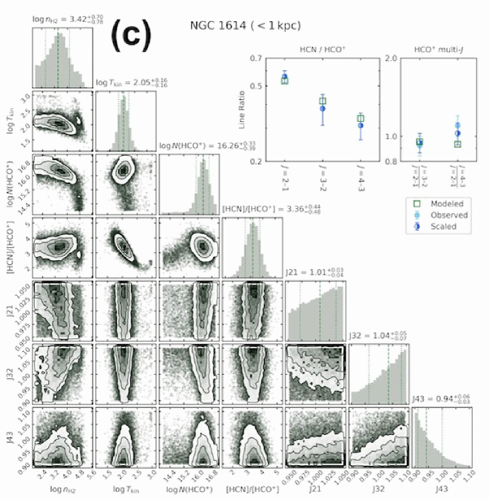
Figure 12: Example result of the MCMC parameter estimation using the HCN-to-HCO⁺ and HCO⁺ multiple J-transition line flux ratios. (a): Central $\lesssim$0.5 kpc region of IRAS 16090$-$0139. (b): Central $\lesssim$0.5 kpc region of IRAS 22491$-$1808. (c): Central $\lesssim$1 kpc region of NGC 1614. The corner plot on the left shows 1D and 2D projections of the posterior distribution for any parameters and parameter pairs, respectively. The median and 68% credible bounds of each parameter are given in the label above each column and are denoted by the dashed and dotted lines, respectively, in the 1D posterior. The panel on the upper right shows a comparison of the observed and modeled emission line flux ratios. The model flux ratios (green open squares) are calculated at the medians of log n${}_{\rm H_{2}}$, log T_kin, log N${}_{\rm HCO^{+}}$, and [HCN]/[HCO⁺]. The observed flux ratios (light blue filled circles) are quoted from Tables 12 and 13 and then scaled with the medians of the J21, J32, and J43 scaling factors (dark blue half-filled circles).

We then compare the posteriors of the gas parameters obtained in different regions of the same (U)LIRG, to illustrate how molecular gas physical parameters spatially change. Figure 13 displays the comparison for three (U)LIRGs as the representatives to discuss the possible spatial variation of some physical parameters. In Figure 13a and 13b, for the two ULIRGs IRAS 16090$-$0139 and IRAS 22491$-$1808, while molecular gas density is estimated to be very high ($\gtrsim$10⁵ cm^-3) at all the $\lesssim$0.5 kpc, $\lesssim$1 kpc, $\lesssim$2 kpc, 0.5–1 kpc, and 1–2 kpc regions, a trend of systematically higher temperature and HCN-to-HCO⁺ abundance ratio at the innermost ($\lesssim$0.5 kpc) regions than the outer nuclear regions (0.5–2 kpc), is seen. Both sources are diagnosed to contain luminous buried AGNs (Table 1 and Figure 8). It is possible that the luminous AGNs create high gas temperature at the innermost part. It is also reported that an HCN-to-HCO⁺ abundance ratio can be enhanced in dense molecular gas in the vicinity of, and affected by, a luminous AGN (e.g., Aladro et al., 2015; Saito et al., 2018; Takano et al., 2019; Nakajima et al., 2018; Kameno et al., 2020; Imanishi et al., 2020; Butterworth et al., 2022; Nakajima et al., 2023). The trend seen in these two ULIRGs can be caused by a luminous AGN.

In Figure 13c, the starburst-dominated LIRG NGC 1614 shows (1) much smaller gas temperature and HCN-to-HCO⁺ abundance ratio than the other two AGN-hosting ULIRGs with the same physical apertures, and (2) no discernible spatial variation of the gas temperature and HCN-to-HCO⁺ abundance ratio at 0.5 kpc physical scales within the central $\lesssim$1 kpc region. These results can naturally be explained by our view that NGC 1614 is energetically dominated by $\sim$1 kpc wide starburst activity, without significant contribution from a central compact luminous AGN (Table 1).

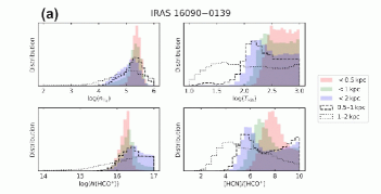
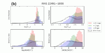
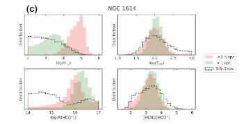
Figure 13: Comparison of the posteriors of gas parameters obtained for different regions in (a): IRAS 16090$-$0139, (b): IRAS 22491$-$1808, and (c): NGC 1614. (Upper left): H₂ gas density in cm^-3. (Upper right): H₂ gas kinetic temperature in K. (Lower left): HCO⁺ column density in cm^-2. (Lower right): HCN-to-HCO⁺ abundance ratio. The red, green, blue filled histograms, and dashed and dotted line histograms correspond to the results for the central $\lesssim$0.5 kpc, $\lesssim$1 kpc, $\lesssim$2 kpc, 0.5–1 kpc annular, and 1–2 kpc annular regions, respectively. Note that the horizontal axis range of the HCN-to-HCO⁺ abundance ratio (Lower right) is much narrower for NGC 1614 than for the other two ULIRGs.

Figure 14 shows the MCMC results for the remaining ULIRGs. The presence of very dense ($\gtrsim$10⁵ cm^-3) and warm ($\gtrsim$300 K) molecular gas is confirmed with this MCMC method in all the regions of all these ULIRGs. For IRAS 00456$-$2904, IRAS 01569$-$2939, and IRAS 03250$+$1606 (Figure 14a–c), there might be a very subtle sign of higher HCN-to-HCO⁺ abundance ratio and/or higher gas temperature at the innermost ($\lesssim$0.5 kpc) region than outer nuclear (0.5–2 kpc) region, but the trend is much weaker than the previously discussed IRAS 16090$-$0139 and IRAS 22491$-$1808 (Figures 13a and 13b). For the remaining ULIRGs, IRAS 00188$-$0856, IRAS 01166$-$0844, and IRAS 22206$-$2715, we see no such trend at all. The absence of such trend can be real, but we note that for ULIRGs for which we have to compare physical parameters among overlapped regions ($\lesssim$0.5 kpc, $\lesssim$1 kpc, and $\lesssim$2 kpc), rather than non-overlapped annular regions ($\lesssim$0.5 kpc, 0.5–1 kpc, and 1–2 kpc), possible spatial variation of gas physical parameters can be diluted if emission is dominated by the innermost $\lesssim$0.5 kpc region ($\S$5.3).

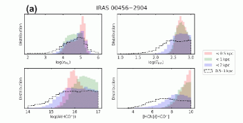
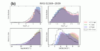
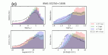
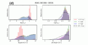
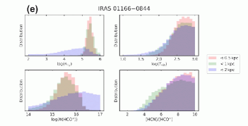
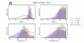
Figure 14: Same as Figure 13, but for (a): IRAS 00456$-$2904, (b): IRAS 01569$-$2939, (c): IRAS 03250$+$1606, (d): IRAS 00188$-$0856, (e): IRAS 01166$-$0844, and (f): IRAS 22206$-$2715. A subtle sign of increasing HCN-to-HCO⁺ abundance ratio and/or increasing temperature toward the innermost $\lesssim$0.5 kpc region is seen in (a)–(c), but not in (d)–(f).

6 Summary

We presented the results of our ALMA $\lesssim$0.5 kpc-resolution, three rotational transition line (J=2–1, J=3–2, and J=4–3) observations of HCN and HCO⁺ for 11 ULIRGs with luminous buried AGN signatures, and one starburst-dominated LIRG NGC 1614. We extracted spectra at the central 0.5 kpc, 1 kpc, and 2 kpc regions, as well as 0.5–1 kpc and 1–2 kpc annular regions, to (1) derive (i) the HCN-to-HCO⁺ flux ratios at J=2–1, J=3–2, and J=4–3, and (ii) high-J to low-J (J=4–3 to J=2–1 and J=3–2 to J=2–1) flux ratios of HCN and HCO⁺, in individual regions, and (2) investigate the possible spatial variations of these ratios among the different regions. We ran RADEX non-LTE model calculations to constrain molecular gas properties for nine (U)LIRGs after excluding three ULIRGs for which (a) not all the J=2–1, J=3–2, and J=4–3 data are available (two sources), and (b) one zone model cannot be applied (one source). We (1) used the Levenberg-Marquardt method by fixing the HCO⁺ column density and HCN-to-HCO⁺ abundance ratio at fiducial values and (2) applied a Bayesian approach by making all parameters free. We found the following main results.

1. HCN and HCO⁺ emission at J=2–1, J=3–2, and J=4–3 were clearly detected in the 0.5 kpc, 1 kpc, and 2 kpc beam-sized spectra of the majority of the observed (U)LIRGs, suggesting the abundant presence of dense and warm molecular gas at the nuclear regions.

2. We quantitatively found that molecular gas at ULIRGs’ innermost ($\lesssim$0.5 kpc) and whole nuclear ($\lesssim$1–2 kpc) regions is very dense ($\gtrsim$10⁵ cm^-3) and warm ($\gtrsim$300 K), and that it is also modestly dense (10^4-4.5 cm^-3) and warm ($\sim$100 K) in one starburst-dominated LIRG’s nucleus ($\lesssim$1 kpc).

3. We saw a signature that the HCN-to-HCO⁺ flux ratios at J=2–1, J=3–2, and J=4–3, and high-J to low-J flux ratios of HCN and HCO⁺, decrease from the innermost ($\lesssim$0.5 kpc) to outer nuclear (0.5–2 kpc) region for some fraction of the observed ULIRGs.

4. For the above ULIRGs showing the signature, we conducted RADEX non-LTE model calculations by freeing all parameters, based on a Bayesian approach, and detected an increasing trend of the HCN-to-HCO⁺ abundance ratio and gas kinetic temperature from the outer nuclear (0.5–2 kpc) to the innermost ($\lesssim$0.5 kpc) regions in two ULIRGs with luminous AGN signatures (IRAS 16090$-$0139 and IRAS 22491$-$1808) significantly and in additional three ULIRGs (IRAS 00456$-$2904, IRAS 01569$-$2939, and IRAS 03250$+$1606) marginally. We interpreted that the trend could naturally be explained by luminous AGN effects to the innermost molecular gas.

5. Our Bayesian approach also demonstrated that the LIRG NGC 1614 displayed (a) much lower gas temperature and HCN-to-HCO⁺ abundance ratio than the observed other nearby ULIRGs’ nuclei, and (b) no discernible spatial change in these two parameters at 0.5 kpc physical scales within the central $\lesssim$1 kpc region. This can naturally be explained by a scenario that NGC 1614 is energetically dominated by $\sim$1 kpc wide starburst activity.

We demonstrated that ALMA multiple molecular, multiple rotational transition line observations, with a combination of non-LTE modeling, are a very unique tool to constrain the spatial variations of physical and chemical properties of molecular gas within nearby (U)LIRGs’ nuclei ($\lesssim$2 kpc), thanks to achievable high spatial resolution ($\lesssim$0.5 kpc) and high sensitivity.

Appendix A Continuum Spectral Energy Distribution

For four ULIRGs, photometric data at 250 $\mu$m, 350 $\mu$m, and 500 $\mu$m, taken with the Herschel Space Observatory, are available (Clements et al., 2018). Figure 15 overplots our ALMA 1 kpc beam-sized continuum flux measurements on the Herschel data as well IRAS 60 $\mu$m and 100 $\mu$m data. Both Herschel and IRAS data were obtained with much larger aperture sizes ($\gtrsim$5^′′ or $\gtrsim$6 kpc at $z\gtrsim$ 0.07) than our ALMA measurements. Infrared 60–500 $\mu$m emission is usually dominated by dust thermal radiation. Our ALMA photometric measurements roughly agree with extrapolation from shorter wavelength IRAS and Herschel data, suggesting that our ALMA 1 kpc beam-sized data cover the bulk of dust thermal radiation from these ULIRGs, as expected from compact ($\lesssim$1 kpc) nature of energetically dominant regions in nearby ULIRGs in general (e.g., Soifer et al., 2000; Diaz-Santos et al., 2010; Imanishi et al., 2011; Pereira-Santaella et al., 2021).

Figure 15: Continuum spectral energy distribution from 60 $\mu$m to $\sim$2000 $\mu$m for four ULIRGs. Herschel 250 $\mu$m, 350 $\mu$m, and 500 $\mu$m (Clements et al., 2018), and IRAS 60 $\mu$m and 100 $\mu$m photometric measurements (Table 1) are displayed as black filled circles. Our ALMA 1 kpc beam-sized continuum flux measurements at 850–2000 $\mu$m (Table 4, column 7) are plotted as open stars. The best-fit graybody curve derived by Clements et al. (2018), using only infrared data at $\lesssim$500 $\mu$m, is overplotted as thick curved line after flux normalization at 250 $\mu$m. Object name and redshift are shown in each panel.

Appendix B Intensity-weighted Mean Velocity (Moment 1) Map

Figure 16 displays the original-beam-sized ($\lesssim$0.5 kpc; Table 3, column 2–4), intensity-weighted mean velocity (moment 1) maps of HCN and HCO⁺ for ULIRGs observed in ALMA Cycle 7, to show dynamical properties of dense molecular line emission. The same maps of other HCN and HCO⁺ J-transition lines for some (U)LIRGs, observed in ALMA Cycle 5 or earlier, have been presented in previous publications (Imanishi & Nakanishi, 2013a; Imanishi et al., 2019, 2022) and thus are not shown here.

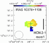
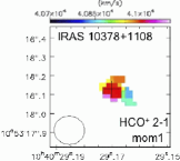
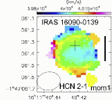
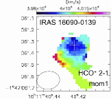
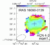
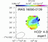
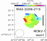
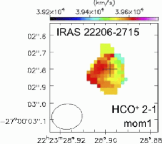
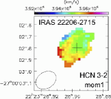
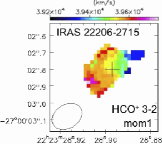
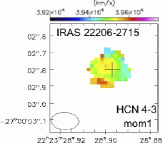
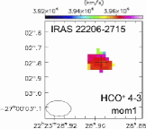
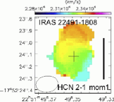
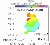
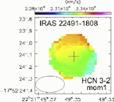
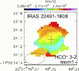
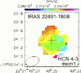
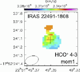
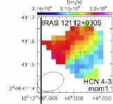
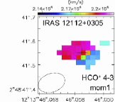
Figure 16: Intensity-weighted mean velocity (moment 1) map of HCN and HCO⁺ lines created from the original-beam-sized data (Table 3, columns 2–4) taken in ALMA Cycle 7. The map of HCO⁺ J=4–3 line for IRAS 03250$+$1606 is not shown because of insufficient S/N ratios. The peak position of the simultaneously taken continuum emission is shown as a cross. For each object, the field of view and velocity display range are set as the same for all lines. The length of the vertical black solid bar in the first image of each object corresponds to 0.5 kpc. Beam size for each moment 1 map is shown as an open circle in the lower-left region.

The moment 1 maps in Figure 16 are created by integrating channels that show significant line signals, relative to continuum flux level. For IRAS 00091$-$0738 and IRAS 22206$-$2715, we see that the HCO⁺ J=4–3 emission line displays distinctly strong redshifted components, compared to other emission lines. We investigate this origin.

It is well known that for sources with non-small molecular line widths ($\gtrsim$300 km s^-1 in full width at half maximum [FWHM]), it is often difficult to clearly separate HCO⁺ and vibrationally excited HCN v₂=1, l=1f (HCN-VIB) emission lines because the latter line is only $\sim$400 km s^-1 redshifted in velocity at the same J-transition (e.g., Aalto et al., 2015b; Imanishi et al., 2016b, 2018; Falstad et al., 2019, 2021). The HCN-VIB emission line flux in units of Jy km s^-1 can be higher at higher J-transition, in the case of thermal excitation. Figure 17 compares the velocity profile of HCN J=4–3 and HCO⁺ J=4–3 lines of IRAS 00091$-$0738 and IRAS 22206$-$2715. IRAS 00091$-$0738 displays significant flux excess at the expected frequency of HCN-VIB J=4–3 at the redshifted side of HCO⁺ J=4–3 (Figure 17a), suggesting that the HCN-VIB J=4–3 emission line is significantly detected and its contamination is a cause of the apparently strong redshifted HCO⁺ J=4–3 emission component in Figure 16. For IRAS 22206$-$2715, however, the signature of the HCN-VIB J=4–3 emission line is not clear, but the blue emission component is weaker for HCO⁺ J=4–3 than for HCN J=4–3 (Figure 17b). The apparently strong redshifted emission component seen in the HCO⁺ J=4–3 moment 1 map (Figure 16) could be explained by the intrinsic velocity difference, possibly caused by different spatial distribution; HCO⁺ emission is usually spatially more extended than HCN emission at the same J-transition in nearby ULIRGs’ nuclei (Imanishi et al. (2019); $\S$4 and Figure 4 of this paper).

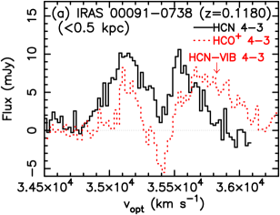
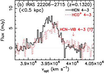
Figure 17: Comparison of velocity profile of HCN J=4–3 (black solid) and HCO⁺ J=4–3 (red dotted) lines for (a) IRAS 00091$-$0738 and (b) IRAS 22206$-$2715 extracted from the 0.5 kpc beam-sized spectra. The abscissa is optical local standard of rest (LSR) velocity in km s^-1 and the ordinate is flux density in mJy. The expected velocity of the HCN-VIB J=4–3 line at the adopted redshift (Table 1, column 2) is indicated with a red downward arrow. The horizontal black dotted straight line indicates the zero flux level.

Appendix C Gaussian fit

Table 9 summarizes the best Gaussian fit of significantly detected HCN and HCO⁺ emission lines at J=2–1, J=3–2, and J=4–3 in the $\lesssim$0.5 kpc, $\lesssim$1 kpc, $\lesssim$2 kpc, 0.5–1 kpc, and 1–2 kpc spectra. For an emission line with only a subtle central dip and/or with possible multiple peaks, but with large data scatters, we adopt a single Gaussian fitting result, after confirming that single and double Gaussian fits provide fluxes which agree well within $\sim$10%. The adopted best Gaussian fits are overplotted to the observed HCN and HCO⁺ emission lines in Figure 18 (for J=2–1), Figure 19 (for J=3–2), and Figure 20 (for J=4–3). These overplots can be used to visually inspect the goodness of the Gaussian fits and check the reliability of our discussion of dense molecular emission line flux ratios.

Table 9: Gaussian Fit of Emission Lines

Object	Region	Molecule	Line	Gaussian fit
				Velocity	Peak	FWHM	Flux
				[km s-1]	[mJy]	[km s-1]	[Jy km s-1]
(1)	(2)	(3)	(4)	(5)	(6)	(7)	(8)
IRAS 00091$-$0738	$\lesssim$0.5 kpc	HCN	J=2–1	35179$\pm$4,35560$\pm$6	4.7$\pm$0.1, 3.6$\pm$0.1	260$\pm$11, 278$\pm$16	2.1$\pm$0.1
			J=3–2	35364$\pm$12, 35392$\pm$8	7.5$\pm$1.0, $-$6.0$\pm$0.9	699$\pm$49, 180$\pm$33	4.0$\pm$0.8
			J=4–3	35132$\pm$10, 35580$\pm$12	9.6$\pm$0.6, 8.3$\pm$0.7	332$\pm$26, 238$\pm$30	4.9$\pm$0.4
		HCO+	J=2–1	35441$\pm$13, 35405$\pm$5	3.3$\pm$0.3, $-$3.9$\pm$0.3	721$\pm$35, 161$\pm$18	1.6$\pm$0.2
			J=3–2	35489$\pm$18, 35414$\pm$7	5.6$\pm$0.9, $-$7.2$\pm$0.9	680$\pm$44, 230$\pm$23	2.1$\pm$0.7
			J=4–3	35533$\pm$25, 35409$\pm$9	8.5$\pm$1.1, $-$11.6$\pm$1.1	766$\pm$52, 241$\pm$24	3.5$\pm$1.0
	$\lesssim$1 kpc	HCN	J=2–1	35183$\pm$9, 35547$\pm$11	5.0$\pm$0.2, 4.1$\pm$0.2	263$\pm$19, 301$\pm$28	2.4$\pm$0.2
			J=3–2	35372$\pm$15, 35397$\pm$9	9.6$\pm$1.5, $-$7.5$\pm$1.2	718$\pm$58, 148$\pm$46	5.5$\pm$1.2
			J=4–3	35129$\pm$18, 35569$\pm$19	11.7$\pm$1.0, 9.5$\pm$1.5	344$\pm$53, 271$\pm$51	6.3$\pm$0.9
		HCO+	J=2–1	35437$\pm$16, 35404$\pm$7	3.8$\pm$0.3, $-$3.8$\pm$0.4	749$\pm$45, 140$\pm$21	2.2$\pm$0.3
			J=3–2	35491$\pm$21, 35415$\pm$9	7.5$\pm$1.4, $-$8.6$\pm$1.3	692$\pm$53, 233$\pm$32	3.0$\pm$1.1 ($<$3$\sigma$)
			J=4–3	35573$\pm$43, 35408$\pm$8	8.1$\pm$0.9, $-$12.6$\pm$1.5	892$\pm$96, 158$\pm$30	5.0$\pm$1.1
	$\lesssim$2 kpc	HCN	J=2–1	35207$\pm$21, 35546$\pm$29	5.6$\pm$0.5, 4.5$\pm$0.5	273$\pm$38, 285$\pm$68	2.7$\pm$0.4
			J=3–2	35373$\pm$18, 35396$\pm$9	12.0$\pm$1.7, $-$10.5$\pm$1.6	676$\pm$54, 122$\pm$40	6.5$\pm$1.3
			J=4–3	35143$\pm$26, 35568$\pm$24	12.4$\pm$1.6, 11.8$\pm$2.6	375$\pm$60, 212$\pm$123	6.8$\pm$1.7
		HCO+	J=2–1	35422$\pm$31, 35405$\pm$12	4.6$\pm$0.7, $-$4.1$\pm$0.9	730$\pm$87, 130$\pm$38	2.7$\pm$0.6
			J=3–2	35173$\pm$21, 35747$\pm$24	6.0$\pm$1.1, 6.9$\pm$0.8	218$\pm$47, 441$\pm$70	4.1$\pm$0.7
			J=4–3	35633$\pm$105, 35406$\pm$10	8.8$\pm$1.2, $-$17.3$\pm$3.0	1145$\pm$246, 115$\pm$31	7.7$\pm$2.5
	0.5–1 kpc	HCN	J=2–1	35397$\pm$29	0.75$\pm$0.11	417$\pm$73	0.30$\pm$0.07
			J=3–2	35189$\pm$29, 35623$\pm$130	2.3$\pm$0.7, 1.7$\pm$0.2	301$\pm$62, 477$\pm$204	1.4$\pm$0.4
			J=4–3	35221$\pm$192	1.8$\pm$0.4	990$\pm$782	1.7$\pm$1.4 ($<$3$\sigma$)
		HCO+	J=2–1	35402$\pm$60	0.74$\pm$0.12	698$\pm$191	0.49$\pm$0.16
			J=3–2	35153$\pm$45, 35733$\pm$51	1.2$\pm$0.4, 1.3$\pm$0.2	286$\pm$127, 488$\pm$136	0.94$\pm$0.27
			J=4–3	35220$\pm$50	2.2$\pm$0.9	257$\pm$117	0.53$\pm$0.34 ($<$3$\sigma$)
	1–2 kpc	HCN	J=2–1	35370$\pm$53	0.95$\pm$0.29	326$\pm$143	0.30$\pm$0.16 ($<$3$\sigma$)
			J=3–2	35379$\pm$66	1.8$\pm$0.3	642$\pm$152	1.1$\pm$0.3
			J=4–3	—	—	—	—
		HCO+	J=2–1	35340$\pm$103	1.0$\pm$0.3	494$\pm$340	0.49$\pm$0.36 ($<$3$\sigma$)
			J=3–2	35613$\pm$113	1.5$\pm$0.4	905$\pm$265	1.3$\pm$0.5 ($<$3$\sigma$)
			J=4–3	—	—	—	—
IRAS 00188$-$0856	$\lesssim$0.5 kpc	HCN	J=2–1	38533$\pm$4	4.7$\pm$0.1	338$\pm$9	1.5$\pm$0.1
			J=3–2	38540$\pm$4	7.7$\pm$0.2	336$\pm$10	2.4$\pm$0.1
			J=4–3	38525$\pm$5	11.1$\pm$0.3	339$\pm$12	3.6$\pm$0.2
		HCO+	J=2–1	38523$\pm$7	2.9$\pm$0.1	303$\pm$14	0.83$\pm$0.05
			J=3–2	38530$\pm$7	4.5$\pm$0.2	328$\pm$14	1.4$\pm$0.1
			J=4–3	38454$\pm$25, 38633$\pm$14	5.8$\pm$0.5, 5.3$\pm$1.4	225$\pm$51, 136$\pm$27	1.9$\pm$0.4
	$\lesssim$1 kpc	HCN	J=2–1	38532$\pm$4	6.8$\pm$0.1	343$\pm$8	2.2$\pm$0.1
			J=3–2	38544$\pm$4	12.7$\pm$0.3	334$\pm$9	4.0$\pm$0.1
			J=4–3	38418$\pm$20, 38611$\pm$23	11.9$\pm$2.6, 14.4$\pm$2.5	195$\pm$40, 220$\pm$32	5.2$\pm$0.9
		HCO+	J=2–1	38519$\pm$7	4.5$\pm$0.2	317$\pm$16	1.4$\pm$0.1
			J=3–2	38528$\pm$7	7.6$\pm$0.3	329$\pm$14	2.4$\pm$0.1
			J=4–3	38449$\pm$27, 38628$\pm$15	8.0$\pm$0.9, 9.3$\pm$1.9	179$\pm$56, 126$\pm$22	2.5$\pm$0.5
	$\lesssim$2 kpc	HCN	J=2–1	38532$\pm$5	8.7$\pm$0.3	348$\pm$13	2.9$\pm$0.1
			J=3–2	38544$\pm$5	16.9$\pm$0.5	337$\pm$12	5.4$\pm$0.3
			J=4–3	38532$\pm$10	20.8$\pm$1.2	371$\pm$25	7.3$\pm$0.6
		HCO+	J=2–1	38519$\pm$10	5.6$\pm$0.3	339$\pm$23	1.8$\pm$0.1
			J=3–2	38517$\pm$9	10.0$\pm$0.5	325$\pm$18	3.1$\pm$0.2
			J=4–3	38519$\pm$24	9.2$\pm$1.4	319$\pm$65	2.8$\pm$0.7
	0.5–1 kpc	HCN	J=2–1	38530$\pm$9	2.1$\pm$0.1	353$\pm$18	0.71$\pm$0.05
			J=3–2	38548$\pm$7	5.0$\pm$0.2	325$\pm$16	1.5$\pm$0.1
			J=4–3	38442$\pm$27, 38633$\pm$41	5.0$\pm$1.2, 5.3$\pm$1.1	166$\pm$34, 172$\pm$37	1.6$\pm$0.4
		HCO+	J=2–1	38510$\pm$13	1.7$\pm$0.1	329$\pm$27	0.53$\pm$0.06
			J=3–2	38524$\pm$10	3.2$\pm$0.2	331$\pm$24	0.98$\pm$0.09
			J=4–3	38414$\pm$12, 38608$\pm$18	2.9$\pm$1.0, 3.0$\pm$0.6	54$\pm$40, 170$\pm$48	0.63$\pm$0.20
	1–2 kpc	HCN	J=2–1	38532$\pm$20	1.8$\pm$0.2	365$\pm$33	0.63$\pm$0.09
			J=3–2	38549$\pm$14	4.2$\pm$0.3	351$\pm$39	1.4$\pm$0.2
			J=4–3	38531$\pm$45	4.4$\pm$0.9	463$\pm$109	1.9$\pm$0.6
		HCO+	J=2–1	38525$\pm$54	1.0$\pm$0.2	483$\pm$143	0.48$\pm$0.16 ($<$3$\sigma$)
			J=3–2	38484$\pm$22	2.5$\pm$0.4	293$\pm$56	0.69$\pm$0.17
			J=4–3	—	—	—	—
IRAS 00456$-$2904	$\lesssim$0.5 kpc	HCN	J=2–1	32938$\pm$3	5.2$\pm$0.1	270$\pm$6	1.3$\pm$0.1
			J=3–2	32937$\pm$5	9.9$\pm$0.3	301$\pm$10	2.9$\pm$0.1
			J=4–3	32934$\pm$4	12.6$\pm$0.4	294$\pm$11	3.6$\pm$0.2
		HCO+	J=2–1	32934$\pm$4	3.6$\pm$0.1	262$\pm$12	0.91$\pm$0.05
			J=3–2	32936$\pm$6	6.0$\pm$0.3	272$\pm$14	1.6$\pm$0.1
			J=4–3	32924$\pm$9	8.1$\pm$0.6	289$\pm$25	2.2$\pm$0.2
	$\lesssim$1 kpc	HCN	J=2–1	32934$\pm$3	7.6$\pm$0.2	281$\pm$7	2.1$\pm$0.1
			J=3–2	32936$\pm$6	14.7$\pm$0.6	307$\pm$13	4.3$\pm$0.3
			J=4–3	32932$\pm$6	17.4$\pm$0.6	309$\pm$14	5.2$\pm$0.3
		HCO+	J=2–1	32925$\pm$4	5.8$\pm$0.2	263$\pm$9	1.5$\pm$0.1
			J=3–2	32931$\pm$8	10.0$\pm$0.6	286$\pm$18	2.8$\pm$0.2
			J=4–3	32940$\pm$11	11.2$\pm$1.0	283$\pm$26	3.0$\pm$0.4
	$\lesssim$2 kpc	HCN	J=2–1	32933$\pm$4	10.3$\pm$0.3	278$\pm$10	2.7$\pm$0.1
			J=3–2	32933$\pm$9	18.5$\pm$1.1	291$\pm$18	5.2$\pm$0.4
			J=4–3	32926$\pm$10	21.0$\pm$1.3	314$\pm$24	6.3$\pm$0.6
		HCO+	J=2–1	32922$\pm$6	8.1$\pm$0.4	261$\pm$14	2.0$\pm$0.1
			J=3–2	32923$\pm$12	14.5$\pm$1.1	296$\pm$24	4.1$\pm$0.5
			J=4–3	32943$\pm$14	17.2$\pm$2.0	222$\pm$35	3.7$\pm$0.7
	0.5–1 kpc	HCN	J=2–1	32926$\pm$7	2.4$\pm$0.1	305$\pm$17	0.72$\pm$0.05
			J=3–2	32936$\pm$13	4.8$\pm$0.4	309$\pm$36	1.4$\pm$0.2
			J=4–3	32853$\pm$13, 33035$\pm$11	5.4$\pm$0.7, 5.2$\pm$0.9	166$\pm$29, 111$\pm$67	1.4$\pm$0.4
		HCO+	J=2–1	32910$\pm$9	2.2$\pm$0.1	260$\pm$22	0.56$\pm$0.06
			J=3–2	32923$\pm$14	4.1$\pm$0.4	299$\pm$28	1.2$\pm$0.2
			J=4–3	32949$\pm$171, 33025$\pm$34	2.5$\pm$1.0, 4.4$\pm$1.9	243 (fix) , 46 (fix)	0.79$\pm$0.24
	1–2 kpc	HCN	J=2–1	32929$\pm$13	2.6$\pm$0.3	269$\pm$29	0.67$\pm$0.10
			J=3–2	32920$\pm$27	3.8$\pm$0.8	239$\pm$63	0.88$\pm$0.29
			J=4–3	32893$\pm$51	3.5$\pm$0.9	351$\pm$115	1.2$\pm$0.5 ($<$3$\sigma$)
		HCO+	J=2–1	32917$\pm$18	2.2$\pm$0.3	267$\pm$38	0.56$\pm$0.12
			J=3–2	32910$\pm$24	4.7$\pm$0.7	300$\pm$65	1.3$\pm$0.4
			J=4–3	32946$\pm$26	5.8$\pm$1.6	159$\pm$59	0.88$\pm$0.41 ($<$3$\sigma$)
IRAS 01166$-$0844	$\lesssim$0.5 kpc	HCN	J=2–1	35139$\pm$8	2.6$\pm$0.1	473$\pm$21	1.2$\pm$0.1
			J=3–2	35151$\pm$15	3.9$\pm$0.2	498$\pm$42	1.8$\pm$0.2
			J=4–3	35161$\pm$10	6.3$\pm$0.3	464$\pm$25	2.8$\pm$0.2
		HCO+	J=2–1	35143$\pm$12	1.8$\pm$0.1	371$\pm$29	0.64$\pm$0.07
			J=3–2	35144$\pm$15	3.5$\pm$0.3	408$\pm$34	1.4$\pm$0.2
			J=4–3	35170$\pm$16	4.3$\pm$0.3	434$\pm$40	1.8$\pm$0.2
	$\lesssim$1 kpc	HCN	J=2–1	35134$\pm$9	3.4$\pm$0.2	433$\pm$27	1.4$\pm$0.1
			J=3–2	35155$\pm$24	5.3$\pm$0.5	586$\pm$80	3.0$\pm$0.5
			J=4–3	35151$\pm$14	7.1$\pm$0.5	454$\pm$35	3.1$\pm$0.3
		HCO+	J=2–1	35129$\pm$12	2.4$\pm$0.2	363$\pm$29	0.84$\pm$0.09
			J=3–2	35127$\pm$19	5.7$\pm$0.5	398$\pm$41	2.2$\pm$0.3
			J=4–3	35162$\pm$18	5.9$\pm$0.5	387$\pm$44	2.2$\pm$0.3
	$\lesssim$2 kpc	HCN	J=2–1	35135$\pm$16	4.2$\pm$0.4	422$\pm$47	1.7$\pm$0.2
			J=3–2	35145$\pm$48	6.1$\pm$0.8	686$\pm$137	4.0$\pm$0.9
			J=4–3	35139$\pm$35	7.1$\pm$1.0	475$\pm$93	3.2$\pm$0.8
		HCO+	J=2–1	35109$\pm$22	2.9$\pm$0.3	441$\pm$65	1.2$\pm$0.2
			J=3–2	35137$\pm$34	6.7$\pm$1.2	375$\pm$75	2.4$\pm$0.6
			J=4–3	35177$\pm$22	9.7$\pm$1.7	245$\pm$62	2.3$\pm$0.7
	0.5–1 kpc	HCN	J=2–1	35105$\pm$15	1.0$\pm$0.2	218$\pm$46	0.21$\pm$0.06
			J=3–2	35154$\pm$93	1.5$\pm$0.3	821$\pm$225	1.2$\pm$0.4
			J=4–3	35077$\pm$231	0.77$\pm$0.31	475$\pm$674	0.35$\pm$0.51 ($<$3$\sigma$)
		HCO+	J=2–1	35096$\pm$28	0.67$\pm$0.16	314$\pm$89	0.20$\pm$0.07 ($<$3$\sigma$)
			J=3–2	35101$\pm$32	2.2$\pm$0.4	385$\pm$72	0.81$\pm$0.20
			J=4–3	35159$\pm$61	1.4$\pm$0.9	272$\pm$119	0.37$\pm$0.28 ($<$3$\sigma$)
	1–2 kpc	HCN	J=2–1	35093$\pm$23	1.3$\pm$0.6	178$\pm$81	0.21$\pm$0.14 ($<$3$\sigma$)
			J=3–2	—	—	—	—
			J=4–3	—	—	—	—
		HCO+	J=2–1	35040$\pm$209	0.60$\pm$0.18	780$\pm$670	0.45$\pm$0.40 ($<$3$\sigma$)
			J=3–2	—	—	—	—
			J=4–3	—	—	—	—
IRAS 01569$-$2939	$\lesssim$0.5 kpc	HCN	J=2–1	41838$\pm$21, 42280$\pm$16	1.4$\pm$0.1, 1.5$\pm$0.2	434$\pm$78, 308$\pm$43	1.0$\pm$0.1
			J=3–2	41854$\pm$22, 42281$\pm$19	2.8$\pm$0.2, 2.9$\pm$0.2	378$\pm$53, 297$\pm$47	1.8$\pm$0.2
			J=4–3	41863$\pm$14, 42285$\pm$12	3.7$\pm$0.2, 3.6$\pm$0.2	400$\pm$32, 276$\pm$26	2.3$\pm$0.2
		HCO+	J=2–1	41823$\pm$27, 42265$\pm$30	1.6$\pm$0.1, 1.5$\pm$0.1	340$\pm$77, 363$\pm$64	1.0$\pm$0.2
			J=3–2	41799$\pm$40, 42243$\pm$54	2.6$\pm$0.5, 2.5$\pm$0.3	388$\pm$65, 491$\pm$93	2.1$\pm$0.3
			J=4–3	41806$\pm$23, 42262$\pm$22	3.3$\pm$0.3, 3.8$\pm$0.2	321$\pm$48, 435$\pm$50	2.5$\pm$0.3
	$\lesssim$1 kpc	HCN	J=2–1	41830$\pm$29, 42284$\pm$29	1.9$\pm$0.1, 1.7$\pm$0.2	412$\pm$67, 373$\pm$54	1.3$\pm$0.2
			J=3–2	41844$\pm$29, 42291$\pm$30	4.4$\pm$0.4, 3.9$\pm$0.5	408$\pm$144, 313$\pm$70	2.8$\pm$0.7
			J=4–3	41865$\pm$16, 42293$\pm$13	5.2$\pm$0.2, 4.6$\pm$0.3	418$\pm$38, 261$\pm$30	3.2$\pm$0.3
		HCO+	J=2–1	41813$\pm$18, 42064$\pm$44	1.4$\pm$0.2, 1.8$\pm$0.1	142$\pm$94, 743$\pm$45	1.5$\pm$0.2
			J=3–2	42004$\pm$18	5.4$\pm$0.3	727$\pm$41	3.7$\pm$0.3
			J=4–3	41804$\pm$24, 42244$\pm$46	5.1$\pm$0.6, 4.5$\pm$0.3	302$\pm$55, 454$\pm$91	3.4$\pm$0.5
	$\lesssim$2 kpc	HCN	J=2–1	42032$\pm$26	2.4$\pm$0.2	798$\pm$63	1.8$\pm$0.2
			J=3–2	41991$\pm$33	5.7$\pm$0.5	707$\pm$70	3.8$\pm$0.5
			J=4–3	41873$\pm$35, 42294$\pm$40	6.5$\pm$0.5, 5.0$\pm$0.8	427$\pm$87, 262$\pm$89	3.8$\pm$0.7
		HCO+	J=2–1	41985$\pm$24	2.8$\pm$0.2	703$\pm$52	1.9$\pm$0.2
			J=3–2	42000$\pm$24	7.1$\pm$0.5	726$\pm$56	4.8$\pm$0.5
			J=4–3	41764$\pm$12, 42144$\pm$66	6.1$\pm$1.0, 5.4$\pm$0.4	179$\pm$75, 646$\pm$120	4.3$\pm$0.8
	0.5–1 kpc	HCN	J=2–1	41952$\pm$57	0.47$\pm$0.09	656$\pm$145	0.29$\pm$0.08
			J=3–2	41954$\pm$48	1.5$\pm$0.2	753$\pm$114	1.0$\pm$0.2
			J=4–3	41984$\pm$44	1.3$\pm$0.2	709$\pm$96	0.87$\pm$0.16
		HCO+	J=2–1	41922$\pm$44	0.67$\pm$0.10	646$\pm$101	0.40$\pm$0.09
			J=3–2	41979$\pm$26	2.5$\pm$0.2	673$\pm$62	1.5$\pm$0.2
			J=4–3	41913$\pm$43	1.6$\pm$0.3	535$\pm$100	0.82$\pm$0.21
	1–2 kpc	HCN	J=2–1	42089$\pm$164	0.48$\pm$0.11	955$\pm$443	0.43$\pm$0.22 ($<$3$\sigma$)
			J=3–2	41940$\pm$78	1.6$\pm$0.4	576$\pm$190	0.84$\pm$0.34 ($<$3$\sigma$)
			J=4–3	41946$\pm$66	1.3$\pm$0.3	543$\pm$167	0.67$\pm$0.26 ($<$3$\sigma$)
		HCO+	J=2–1	41956$\pm$67	0.70$\pm$0.14	620$\pm$156	0.40$\pm$0.13
			J=3–2	41987$\pm$70	1.6$\pm$0.3	724$\pm$186	1.1$\pm$0.35
			J=4–3	41897$\pm$89	1.3$\pm$0.5	768$\pm$302	0.94$\pm$0.54 ($<$3$\sigma$)
IRAS 03250$+$1606	$\lesssim$0.5 kpc	HCN	J=2–1	38607$\pm$21	1.2$\pm$0.1	582$\pm$49	0.67$\pm$0.07
			J=3–2	38407$\pm$10, 38700$\pm$30	2.6$\pm$0.4, 2.2$\pm$0.2	130$\pm$34, 453$\pm$50	1.3$\pm$0.2
			J=4–3	38443$\pm$20, 38780$\pm$38	2.7$\pm$0.4, 2.2$\pm$0.2	199$\pm$40, 317$\pm$84	1.2$\pm$0.2
		HCO+	J=2–1	38607$\pm$32	0.94$\pm$0.10	533$\pm$71	0.47$\pm$0.08
			J=3–2	38449$\pm$23, 38751$\pm$43	2.1$\pm$0.3, 1.8$\pm$0.2	221$\pm$76, 279$\pm$77	0.92$\pm$0.22
			J=4–3	38505$\pm$35, 38844$\pm$62	2.2$\pm$0.3, 1.8$\pm$0.3	287$\pm$78, 212$\pm$132	0.97$\pm$0.30
	$\lesssim$1 kpc	HCN	J=2–1	38615$\pm$20	1.9$\pm$0.1	583$\pm$43	1.1$\pm$0.1
			J=3–2	38455$\pm$25, 38800$\pm$52	4.6$\pm$0.4, 3.5$\pm$0.4	233$\pm$55, 298$\pm$95	2.0$\pm$0.4
			J=4–3	38445$\pm$32, 38793$\pm$62	4.1$\pm$0.6, 3.7$\pm$0.4	240$\pm$80, 309$\pm$126	2.0$\pm$0.6
		HCO+	J=2–1	38614$\pm$26	1.7$\pm$0.1	577$\pm$53	0.92$\pm$0.12
			J=3–2	38447$\pm$23, 38769$\pm$34	3.5$\pm$0.5, 3.7$\pm$0.3	210$\pm$83, 295$\pm$69	1.7$\pm$0.4
			J=4–3	38463$\pm$36, 38780$\pm$23	3.7$\pm$0.7, 3.9$\pm$0.5	148$\pm$94, 309$\pm$62	1.6$\pm$0.4
	$\lesssim$2 kpc	HCN	J=2–1	38580$\pm$24	2.7$\pm$0.2	512$\pm$55	1.3$\pm$0.2
			J=3–2	38601$\pm$27	5.2$\pm$0.6	555$\pm$55	2.7$\pm$0.4
			J=4–3	38423$\pm$30, 38796$\pm$39	4.9$\pm$0.9, 4.9$\pm$0.8	205$\pm$81, 316$\pm$81	2.4$\pm$0.6
		HCO+	J=2–1	38638$\pm$38	2.4$\pm$0.3	659$\pm$85	1.5$\pm$0.3
			J=3–2	38665$\pm$23	5.5$\pm$0.5	509$\pm$51	2.6$\pm$0.3
			J=4–3	38452$\pm$121, 38761$\pm$34	4.5$\pm$1.6, 5.8$\pm$1.0	137$\pm$176, 305$\pm$72	2.3$\pm$0.9 ($<$3$\sigma$)
	0.5–1 kpc	HCN	J=2–1	38626$\pm$38	0.71$\pm$0.09	581$\pm$93	0.39$\pm$0.08
			J=3–2	38481$\pm$24, 38834$\pm$29	1.8$\pm$0.2, 1.5$\pm$0.3	240$\pm$65, 223$\pm$78	0.71$\pm$0.17
			J=4–3	38634$\pm$40	1.6$\pm$0.2	575$\pm$94	0.86$\pm$0.17
		HCO+	J=2–1	38629$\pm$49	0.78$\pm$0.11	605$\pm$130	0.44$\pm$0.12
			J=3–2	38456$\pm$42, 38796$\pm$49	1.4$\pm$0.4, 1.9$\pm$0.2	217$\pm$133, 283$\pm$56	0.80$\pm$0.23
			J=4–3	38757$\pm$34	1.9$\pm$0.5	366$\pm$90	0.66$\pm$0.23 ($<$3$\sigma$)
	1–2 kpc	HCN	J=2–1	38529$\pm$58	0.79$\pm$0.22	372$\pm$136	0.28$\pm$0.13 ($<$3$\sigma$)
			J=3–2	38592$\pm$68	1.3$\pm$0.6	555$\pm$112	0.70$\pm$0.33 ($<$3$\sigma$)
			J=4–3	—	—	—	—
		HCO+	J=2–1	38676$\pm$133	0.76$\pm$0.22	854$\pm$253	0.61$\pm$0.25 ($<$3$\sigma$)
			J=3–2	38715$\pm$34	2.1$\pm$0.3	440$\pm$89	0.85$\pm$0.21
			J=4–3	38725$\pm$63	1.9$\pm$0.8	306$\pm$149	0.56$\pm$0.36 ($<$3$\sigma$)
IRAS 10378$+$1108	$\lesssim$0.5 kpc	HCN	J=2–1	40913$\pm$9	2.8$\pm$0.2	342$\pm$24	0.90$\pm$0.08
			J=3–2	40934$\pm$4	7.2$\pm$0.2	402$\pm$11	2.7$\pm$0.1
		HCO+	J=2–1	40930$\pm$13	2.3$\pm$0.2	373$\pm$34	0.82$\pm$0.09
			J=3–2	40934$\pm$5	6.9$\pm$0.2	381$\pm$12	2.5$\pm$0.1
	$\lesssim$1 kpc	HCN	J=2–1	40896$\pm$8	4.7$\pm$0.2	341$\pm$18	1.5$\pm$0.1
			J=3–2	40915$\pm$5	11.3$\pm$0.3	383$\pm$13	4.1$\pm$0.2
		HCO+	J=2–1	40906$\pm$12	4.3$\pm$0.3	388$\pm$27	1.6$\pm$0.1
			J=3–2	40916$\pm$5	11.3$\pm$0.3	362$\pm$12	3.8$\pm$0.2
	$\lesssim$2 kpc	HCN	J=2–1	40892$\pm$10	7.3$\pm$0.5	327$\pm$24	2.2$\pm$0.2
			J=3–2	40913$\pm$7	14.3$\pm$0.7	388$\pm$20	5.2$\pm$0.4
		HCO+	J=2–1	40907$\pm$16	6.4$\pm$0.5	427$\pm$46	2.6$\pm$0.3
			J=3–2	40906$\pm$9	14.5$\pm$0.6	366$\pm$21	5.0$\pm$0.4
	0.5–1 kpc	HCN	J=2–1	40869$\pm$15	1.9$\pm$0.2	312$\pm$44	0.56$\pm$0.09
			J=3–2	40886$\pm$9	4.2$\pm$0.3	339$\pm$24	1.3$\pm$0.1
		HCO+	J=2–1	40879$\pm$19	2.0$\pm$0.2	385$\pm$47	0.72$\pm$0.13
			J=3–2	40889$\pm$10	4.5$\pm$0.3	328$\pm$28	1.4$\pm$0.1
	1–2 kpc	HCN	J=2–1	40886$\pm$21	2.7$\pm$0.4	294$\pm$58	0.73$\pm$0.18
			J=3–2	40903$\pm$23	3.1$\pm$0.4	403$\pm$63	1.2$\pm$0.2
		HCO+	J=2–1	40903$\pm$43	2.1$\pm$0.3	535$\pm$117	1.1$\pm$0.3
			J=3–2	40872$\pm$27	3.3$\pm$0.5	357$\pm$66	1.1$\pm$0.3
IRAS 16090$-$0139	$\lesssim$0.5 kpc	HCN	J=2–1	40036$\pm$7	4.4$\pm$0.1	570$\pm$17	2.4$\pm$0.1
			J=3–2	40041$\pm$7	8.0$\pm$0.2	538$\pm$18	4.1$\pm$0.2
			J=4–3	40017$\pm$5	15.8$\pm$0.3	556$\pm$12	8.3$\pm$0.2
		HCO+	J=2–1	39998$\pm$14	3.2$\pm$0.1	624$\pm$36	1.9$\pm$0.1
			J=3–2	40035$\pm$13	6.2$\pm$0.3	570$\pm$31	3.3$\pm$0.2
			J=4–3	40021$\pm$5	12.8$\pm$0.3	480$\pm$11	5.8$\pm$0.2
	$\lesssim$1 kpc	HCN	J=2–1	40052$\pm$5	7.9$\pm$0.2	537$\pm$12	4.0$\pm$0.1
			J=3–2	40054$\pm$9	13.6$\pm$0.4	540$\pm$20	6.9$\pm$0.3
			J=4–3	40043$\pm$5	23.5$\pm$0.5	572$\pm$13	12.6$\pm$0.4
		HCO+	J=2–1	40030$\pm$7	6.2$\pm$0.2	579$\pm$18	3.4$\pm$0.1
			J=3–2	40066$\pm$13	12.0$\pm$0.5	576$\pm$31	6.5$\pm$0.4
			J=4–3	40050$\pm$5	19.9$\pm$0.4	505$\pm$27	9.4$\pm$0.5
	$\lesssim$2 kpc	HCN	J=2–1	40064$\pm$7	11.5$\pm$0.3	487$\pm$18	5.3$\pm$0.2
			J=3–2	40057$\pm$12	18.6$\pm$0.8	541$\pm$28	9.5$\pm$0.6
			J=4–3	40042$\pm$9	29.0$\pm$0.9	570$\pm$21	15.5$\pm$0.7
		HCO+	J=2–1	40072$\pm$10	9.4$\pm$0.4	569$\pm$24	5.0$\pm$0.3
			J=3–2	40087$\pm$13	18.5$\pm$0.9	596$\pm$30	10.3$\pm$0.7
			J=4–3	40069$\pm$8	26.2$\pm$0.9	490$\pm$20	12.1$\pm$0.6
	0.5–1 kpc	HCN	J=2–1	40070$\pm$9	3.6$\pm$0.1	483$\pm$21	1.6$\pm$0.1
			J=3–2	40072$\pm$13	5.6$\pm$0.3	535$\pm$32	2.8$\pm$0.2
			J=4–3	40094$\pm$11	7.9$\pm$0.3	580$\pm$29	4.3$\pm$0.3
		HCO+	J=2–1	40061$\pm$11	3.2$\pm$0.1	495$\pm$27	1.5$\pm$0.1
			J=3–2	40094$\pm$15	5.9$\pm$0.3	581$\pm$32	3.2$\pm$0.2
			J=4–3	40104$\pm$10	7.4$\pm$0.3	523$\pm$25	3.6$\pm$0.2
	1–2 kpc	HCN	J=2–1	40091$\pm$15	3.8$\pm$0.3	389$\pm$34	1.4$\pm$0.2
			J=3–2	40065$\pm$28	5.0$\pm$0.5	544$\pm$72	2.5$\pm$0.4
			J=4–3	40039$\pm$29	5.5$\pm$0.7	556$\pm$89	2.9$\pm$0.6
		HCO+	J=2–1	40143$\pm$16	3.8$\pm$0.3	432$\pm$47	1.5$\pm$0.2
			J=3–2	40129$\pm$25	6.8$\pm$0.6	587$\pm$59	3.7$\pm$0.5
			J=4–3	40133$\pm$20	7.4$\pm$0.7	358$\pm$48	2.5$\pm$0.4
IRAS 22206$-$2715	$\lesssim$0.5 kpc	HCN	J=2–1	39496$\pm$7	3.1$\pm$0.1	439$\pm$16	1.3$\pm$0.1
			J=3–2	39495$\pm$8	5.2$\pm$0.2	420$\pm$18	2.1$\pm$0.1
			J=4–3	39492$\pm$9	7.2$\pm$0.3	417$\pm$22	2.8$\pm$0.2
		HCO+	J=2–1	39524$\pm$12	2.2$\pm$0.1	423$\pm$29	0.86$\pm$0.08
			J=3–2	39517$\pm$10	3.7$\pm$0.2	438$\pm$24	1.5$\pm$0.1
			J=4–3	39545$\pm$14	4.9$\pm$0.3	479$\pm$37	2.2$\pm$0.2
	$\lesssim$1 kpc	HCN	J=2–1	39493$\pm$6	4.7$\pm$0.1	398$\pm$14	1.8$\pm$0.1
			J=3–2	39500$\pm$7	7.4$\pm$0.2	432$\pm$17	3.0$\pm$0.2
			J=4–3	39481$\pm$10	9.8$\pm$0.5	430$\pm$24	4.0$\pm$0.3
		HCO+	J=2–1	39517$\pm$10	3.6$\pm$0.2	361$\pm$24	1.2$\pm$0.1
			J=3–2	39513$\pm$10	5.6$\pm$0.3	412$\pm$23	2.2$\pm$0.2
			J=4–3	39508$\pm$15	7.0$\pm$0.5	424$\pm$36	2.8$\pm$0.3
	$\lesssim$2 kpc	HCN	J=2–1	39489$\pm$9	6.7$\pm$0.3	373$\pm$21	2.4$\pm$0.2
			J=3–2	39513$\pm$11	9.3$\pm$0.5	463$\pm$29	4.1$\pm$0.3
			J=4–3	39470$\pm$20	12.6$\pm$1.2	423$\pm$42	5.0$\pm$0.7
		HCO+	J=2–1	39523$\pm$12	5.1$\pm$0.5	270$\pm$34	1.3$\pm$0.2
			J=3–2	39508$\pm$13	7.4$\pm$0.5	383$\pm$30	2.7$\pm$0.3
			J=4–3	39515$\pm$34	9.3$\pm$1.1	493$\pm$83	4.3$\pm$0.9
	0.5–1 kpc	HCN	J=2–1	39482$\pm$10	1.7$\pm$0.1	317$\pm$25	0.51$\pm$0.05
			J=3–2	39518$\pm$20	2.2$\pm$0.2	474$\pm$53	0.99$\pm$0.14
			J=4–3	39450$\pm$31	2.6$\pm$0.3	460$\pm$65	1.1$\pm$0.2
		HCO+	J=2–1	39506$\pm$16	1.5$\pm$0.2	259$\pm$43	0.35$\pm$0.08
			J=3–2	39506$\pm$18	1.9$\pm$0.2	349$\pm$46	0.61$\pm$0.11
			J=4–3	39422$\pm$23	3.2$\pm$0.7	212$\pm$54	0.63$\pm$0.21
	1–2 kpc	HCN	J=2–1	39477$\pm$20	2.0$\pm$0.3	306$\pm$50	0.58$\pm$0.13
			J=3–2	39601$\pm$74	1.9$\pm$0.3	669$\pm$196	1.2$\pm$0.4
			J=4–3	39435$\pm$84	2.4$\pm$1.1	474$\pm$140	1.1$\pm$0.6 ($<$3$\sigma$)
		HCO+	J=2–1	39523$\pm$12	2.3$\pm$0.6	109$\pm$42	0.23$\pm$0.11 ($<$3$\sigma$)
			J=3–2	39499$\pm$38	1.8$\pm$0.5	277$\pm$113	0.48$\pm$0.23 ($<$3$\sigma$)
			J=4–3	39550$\pm$137	2.4$\pm$0.7	695$\pm$295	1.6$\pm$0.8 ($<$3$\sigma$)
IRAS 22491$-$1808	$\lesssim$0.5 kpc	HCN	J=2–1	23303$\pm$4	10.8$\pm$0.2	452$\pm$9	4.8$\pm$0.1
			J=3–2	23310$\pm$5	18.6$\pm$0.4	499$\pm$13	9.2$\pm$0.3
			J=4–3	23305$\pm$6	24.4$\pm$0.6	514$\pm$14	12.4$\pm$0.4
		HCO+	J=2–1	23276$\pm$8	6.6$\pm$0.2	490$\pm$17	3.2$\pm$0.1
			J=3–2	23334$\pm$12	10.9$\pm$0.4	592$\pm$24	6.4$\pm$0.3
			J=4–3	23333$\pm$16	13.4$\pm$0.6	626$\pm$34	8.3$\pm$0.6
	$\lesssim$1 kpc	HCN	J=2–1	23311$\pm$5	14.1$\pm$0.4	425$\pm$12	5.9$\pm$0.2
			J=3–2	23323$\pm$6	22.9$\pm$0.6	474$\pm$14	10.7$\pm$0.4
			J=4–3	23303$\pm$10	31.4$\pm$1.2	505$\pm$22	15.7$\pm$0.9
		HCO+	J=2–1	23295$\pm$8	9.4$\pm$0.3	442$\pm$18	4.1$\pm$0.2
			J=3–2	23341$\pm$12	14.3$\pm$0.6	525$\pm$28	7.4$\pm$0.5
			J=4–3	23356$\pm$22	20.2$\pm$1.2	656$\pm$51	13.1$\pm$1.3
	$\lesssim$2 kpc	HCN	J=2–1	23313$\pm$10	16.4$\pm$0.9	385$\pm$23	6.2$\pm$0.5
			J=3–2	23326$\pm$11	25.6$\pm$1.2	464$\pm$26	11.8$\pm$0.9
			J=4–3	23306$\pm$23	29.6$\pm$2.6	502$\pm$52	14.7$\pm$2.0
		HCO+	J=2–1	23308$\pm$14	12.0$\pm$0.9	388$\pm$32	4.6$\pm$0.5
			J=3–2	23354$\pm$18	17.5$\pm$1.2	485$\pm$40	8.4$\pm$0.9
			J=4–3	23352$\pm$38	26.7$\pm$2.8	612$\pm$99	16.1$\pm$3.1
	0.5–1 kpc	HCN	J=2–1	23345$\pm$15	3.5$\pm$0.3	325$\pm$33	1.1$\pm$0.2
			J=3–2	23371$\pm$18	4.8$\pm$0.6	325$\pm$50	1.6$\pm$0.3
			J=4–3	23296$\pm$32	7.0$\pm$0.9	482$\pm$74	3.3$\pm$0.7
		HCO+	J=2–1	23343$\pm$16	3.3$\pm$0.3	292$\pm$38	0.95$\pm$0.16
			J=3–2	23369$\pm$24	3.8$\pm$0.7	326$\pm$65	1.2$\pm$0.3
			J=4–3	23351$\pm$37	7.4$\pm$0.9	575$\pm$98	4.2$\pm$0.9
	1–2 kpc	HCN	J=2–1	23344$\pm$38	2.9$\pm$1.0	174$\pm$94	0.50$\pm$0.33 ($<$3$\sigma$)
			J=3–2	—	—	—	—
			J=4–3	—	—	—	—
		HCO+	J=2–1	23381$\pm$24	4.3$\pm$1.1	131$\pm$39	0.56$\pm$0.22 ($<$3$\sigma$)
			J=3–2	—	—	—	—
			J=4–3	—	—	—	—
IRAS 12112$+$0305	$\lesssim$0.5 kpc	HCN	J=4–3	21668$\pm$15, 21985$\pm$9	22.3$\pm$1.6, 25.3$\pm$1.9	301$\pm$38, 199$\pm$23	11.6$\pm$1.2
		HCO+	J=4–3	21643$\pm$13, 22013$\pm$17	12.6$\pm$1.5, 13.8$\pm$1.2	181$\pm$33, 321$\pm$58	6.7$\pm$1.0
	$\lesssim$1 kpc	HCN	J=4–3	21835$\pm$17	31.5$\pm$1.9	587$\pm$38	18.4$\pm$1.6
		HCO+	J=4–3	21975$\pm$35	17.0$\pm$1.7	670$\pm$80	11.3$\pm$1.8
	$\lesssim$2 kpc	HCN	J=4–3	21861$\pm$32	34.0$\pm$3.5	580$\pm$89	19.6$\pm$3.6
		HCO+	J=4–3	22031$\pm$46	23.3$\pm$3.7	561$\pm$110	13.0$\pm$3.3
	0.5–1 kpc	HCN	J=4–3	21885$\pm$40	9.6$\pm$1.3	574$\pm$143	5.5$\pm$1.6
		HCO+	J=4–3	21900 (fix)	5.0$\pm$1.3	568$\pm$357	2.8$\pm$1.9 ($<$3$\sigma$)
	1–2 kpc	HCN	J=4–3	—	—	—	—
		HCO+	J=4–3	—	—	—	—
NGC 1614	$\lesssim$0.5 kpc	HCN	J=2–1	4763$\pm$4	14.2$\pm$0.5	222$\pm$8	3.3$\pm$0.2
			J=3–2	4762$\pm$11	11.9$\pm$1.3	209$\pm$25	2.6$\pm$0.4
			J=4–3	4779$\pm$10	12.2$\pm$1.2	208$\pm$23	2.6$\pm$0.4
		HCO+	J=2–1	4767$\pm$3	23.1$\pm$0.5	229$\pm$7	5.5$\pm$0.2
			J=3–2	4753$\pm$7	24.1$\pm$1.5	233$\pm$13	5.9$\pm$0.5
			J=4–3	4776$\pm$6	38.7$\pm$2.2	211$\pm$13	8.5$\pm$0.7
	$\lesssim$1 kpc	HCN	J=2–1	4765$\pm$4	26.9$\pm$0.9	243$\pm$10	6.8$\pm$0.4
			J=3–2	4776$\pm$14	16.5$\pm$1.9	245$\pm$34	4.2$\pm$0.8
			J=4–3	4769$\pm$10	16.3$\pm$1.3	252$\pm$24	4.3$\pm$0.5
		HCO+	J=2–1	4769$\pm$4	46.7$\pm$1.2	252$\pm$8	12.3$\pm$0.5
			J=3–2	4757$\pm$8	42.1$\pm$2.5	256$\pm$13	11.3$\pm$0.9
			J=4–3	4773$\pm$7	55.4$\pm$3.0	240$\pm$16	13.9$\pm$1.2
	0.5–1 kpc	HCN	J=2–1	4767$\pm$6	12.9$\pm$0.6	259$\pm$16	3.5$\pm$0.3
			J=3–2	4835$\pm$41	5.4$\pm$1.4	272$\pm$107	1.6$\pm$0.7 ($<$3$\sigma$)
			J=4–3	4712$\pm$34	4.5$\pm$0.7	425$\pm$73	2.0$\pm$0.5
		HCO+	J=2–1	4772$\pm$4	23.8$\pm$0.7	274$\pm$9	6.8$\pm$0.3
			J=3–2	4661$\pm$10, 4840$\pm$12	18.6$\pm$2.1, 19.6$\pm$1.9	119$\pm$19, 148$\pm$22	5.4$\pm$0.7
			J=4–3	4653$\pm$13, 4842$\pm$9	19.9$\pm$2.1, 24.4$\pm$2.6	109$\pm$26, 117$\pm$30	5.3$\pm$1.0

Note. — Col.(1): Object name. Col.(2): Region. Col.(3): Molecule. Col.(4): J-transition. Cols.(5)–(8): Gaussian fit of emission line. “—” means that no Gaussian fit is applied, because of no emission line signature in a spectrum. Col.(5): Optical LSR velocity (v_opt) of emission line peak in km s^-1. Col.(6): Peak flux in mJy. Col.(7): Observed full width at half maximum (FWHM) in km s^-1. Col.(8): Gaussian-fit velocity-integrated flux in Jy km s^-1. When fitting results of two Gaussian components are adopted, fluxes of the two components are added. Only Gaussian fitting error (statistical uncertainty) is considered.

Figure 18: Adopted Gaussian fits (solid curved lines) of the HCN and HCO⁺ J=2–1 emission lines extracted in the 0.5 kpc (left two panels), 1 kpc (middle two panels), and 2 kpc (right two panels) beam-sized spectra in the first row for each ULIRG. In the second row, those extracted from the spectra of 0.5–1 kpc (left two panels) and 1–2 kpc (middle two panels) annular regions are shown. For the LIRG NGC 1614, only those from the spectra of the central $\lesssim$0.5 kpc (left two panels), $\lesssim$1 kpc (middle two panels), and 0.5–1 kpc annular (right two panels) regions are displayed. The abscissa is optical LSR velocity in km s^-1 and the ordinate is flux density in mJy. The horizontal thin dotted straight line indicates the zero flux level.

Figure 19: Same as Figure 18, but for the J=3–2 lines of HCN and HCO⁺. No Gaussian fit is applied when there is no emission line signature at all, particularly in the 1–2 kpc annular region spectra.

Figure 20: Same as Figure 18, but for the J=4–3 lines of HCN and HCO⁺. No Gaussian fit is applied when there is no emission line signature at all, particularly in the 1–2 kpc annular region spectra.

Appendix D CS J=7–6 line

The CS J=7–6 ($\nu_{\rm rest}$=342.883 GHz) emission line was serendipitously detected in all ULIRGs for which HCN and HCO⁺ J=4–3 observations were made. Figure 21 shows the integrated intensity (moment 0) maps of CS J=7–6 created from the original-beam-sized data (Table 3; column 4). Figure 22 displays the 0.5 kpc beam-sized spectra that include the CS J=7–6 line. Table 10 summarizes the best fit Gaussian parameters for the CS J=7–6 emission line detected in the 0.5 kpc beam-sized spectra. Figure 23 overplots the best fit Gaussian on the observed CS J=7–6 emission line in the 0.5 kpc beam-sized spectra. The CS J=7–6 emission line was not detected in the LIRG NGC 1614 (Imanishi & Nakanishi, 2013a).

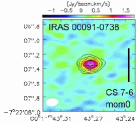
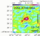
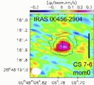
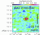
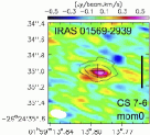
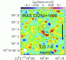
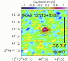
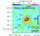
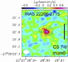
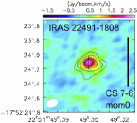
Figure 21: Integrated intensity (moment 0) map of the CS J=7–6 line created from the original-beam-sized data (Table 3, column 4). Continuum emission that was simultaneously obtained (J43) is shown as contours. The contours start from 4$\sigma$ and increase by a factor of 2 (i.e., 8$\sigma$, 16$\sigma$, 32$\sigma$, and 64$\sigma$) for all ULIRGs. Continuum peak position is shown as a cross. The length of the vertical black solid bar at the right side of each object corresponds to 1 kpc. Beam size for each moment 0 map is shown as a white filled circle in the lower-left region.

Figure 22: 0.5 kpc beam-sized spectrum that includes the CS J=7–6 line, taken during the J43 observation. The abscissa is observed frequency in GHz and the ordinate is flux density in mJy. An upward arrow is placed at the expected observed frequency of CS J=7–6 for the adopted redshift (Table 1, column 2). The horizontal thin dotted straight line indicates the zero flux level.

Table 10: Gaussian Fit of CS J=7–6 Emission Line Extracted from the 0.5 kpc Beam-sized Spectra

Object	Gaussian fit
	Velocity	Peak	FWHM	Flux
	[km s-1]	[mJy]	[km s-1]	[Jy km s-1]
(1)	(2)	(3)	(4)	(5)
IRAS 00091$-$0738	35145$\pm$10, 35529$\pm$15	4.7$\pm$0.4, 4.2$\pm$0.4	199$\pm$23, 358$\pm$41	2.3$\pm$0.2
IRAS 00188$-$0856	38403$\pm$13, 38620$\pm$26	2.7$\pm$0.3, 1.8$\pm$0.4	157$\pm$35, 152$\pm$58	0.65$\pm$0.15
IRAS 00456$-$2904	32940$\pm$15	2.4$\pm$0.3	201$\pm$36	0.46$\pm$0.10
IRAS 01166$-$0844	35137$\pm$26	2.0$\pm$0.2	467$\pm$67	0.87$\pm$0.16
IRAS 01569$-$2939	41960$\pm$53	1.0$\pm$0.2	624$\pm$126	0.59$\pm$0.15
IRAS 16090$-$0139	39994$\pm$15	4.1$\pm$0.3	393$\pm$52	1.5$\pm$0.2
IRAS 22206$-$2715	39300$\pm$10, 39573$\pm$34	3.5$\pm$0.8, 2.4$\pm$0.4	96$\pm$29, 255$\pm$59	0.88$\pm$0.20
IRAS 22491$-$1808	23292$\pm$12	10$\pm$1	464$\pm$27	4.6$\pm$0.3
IRAS 12112$+$0305	21636$\pm$16, 21970$\pm$14	6.7$\pm$1.0, 8.1$\pm$1.8	195$\pm$42, 131$\pm$31	2.4$\pm$0.5

Note. — Col.(1): Object name. Cols.(2)–(5): Gaussian fit of the CS J=7–6 emission line detected in the 0.5 kpc beam-sized spectrum. Col.(2): Optical LSR velocity (v_opt) of emission line peak in km s^-1. Col.(3): Peak flux in mJy. Col.(4): Observed FWHM in km s^-1. Col.(5): Gaussian-fit velocity-integrated flux in Jy km s^-1. When fitting results of two Gaussian components are adopted, fluxes of the two components are added. Only Gaussian fitting error (statistical uncertainty) is considered.

Figure 23: Adopted Gaussian fit (solid curved line) of the CS J=7–6 emission line in the 0.5 kpc beam-sized spectra for sources with significant detection (all ULIRGs except IRAS 03250$+$1606). The abscissa is optical LSR velocity in km s^-1 and the ordinate is flux density in mJy. The horizontal thin dotted straight line indicates the zero flux level.

Appendix E HC₃N line

HC₃N J=18–17 ($\nu_{\rm rest}$=163.753 GHz) or J=21–20 ($\nu_{\rm rest}$=191.040 GHz) emission lines were serendipitously detected in some ULIRGs during the observations of HCN and HCO⁺ J=2–1. Figure 24 shows the integrated intensity (moment 0) maps of HC₃N J=18–17 or J=21–20 created from the original-beam-sized data (Table 3; column 2). Figure 25 displays the 0.5 kpc beam-sized spectra that include the HC₃N J=18–17 or J=21–20 line. The best fit Gaussian parameters for these HC₃N emission lines extracted from the 0.5 kpc beam-sized spectra are summarized in Table 11. In Figure 26, the best fit Gaussian is overplotted to the observed HC₃N emission line in the 0.5 kpc beam-sized spectra. No HC₃N line was covered in the spectrum of the LIRG NGC 1614 (Imanishi et al., 2022).

When compared to other dense molecular lines, HC₃N emission can be strong in galaxies with high column density of obscuring material around energy sources (Aalto et al., 2007; Lindberg et al., 2011), because HC₃N is strongly emitted in UV-shielded regions at some distance from the energy sources (Lindberg et al., 2011; Meier et al., 2011). Lindberg et al. (2011) defined HC₃N-luminous galaxies as sources with HC₃N J=10–9 to HCN J=1–0 flux ratio of $>$0.15, which constitute less than one-third of observed galaxies, including those with much less infrared luminosity than (U)LIRGs. The rest frequency ($\nu_{\rm rest}$) of HC₃N J=20–19 and HCN J=2–1 that we observed is approximately twice that of HC₃N J=10–9 and HCN J=1–0, respectively. If emission is thermalized and optically thick, where flux in units of Jy km s^-1 increases with $\nu_{\rm rest}$², then the HC₃N J=20–19 to HCN J=2–1 flux ratios are expected to be comparable to the HC₃N J=10–9 to HCN J=1–0 flux ratios. However, the upper excitation energy level for HC₃N J=20–19 (E_u $\sim$ 92 K) is significantly higher than those of HCN J=2–1 (E_u $\sim$ 13 K), HC₃N J=10–9 (24 K), and HCN J=1–0 (4 K). If only HC₃N J=20–19 is significantly sub-thermally excited than other three lines, then the HC₃N J=20–19 to HCN J=2–1 flux ratio can be smaller than the HC₃N J=10–9 to HCN J=1–0 flux ratio. In this sense, a source is safely classified as a HC₃N-luminous galaxy, if the HC₃N J=20–19 to HCN J=2–1 flux ratio is larger than 0.15. IRAS 00091$-$0738 corresponds to this case (Table 11, column 7). The strong self-absorption of HCO⁺ and HCN lines at J=2–1, J=3–2, and J=4–3, detected in IRAS 00091$-$0738 (Figure 2), suggests the presence of large column density of obscuring material at the foreground side of a background 0.85–2 mm continuum emitting energy source. The bright HC₃N emission observed in IRAS 00091$-$0738 can come from highly shielded regions.

For the remaining ULIRGs, the observed HC₃N J=20–19 to HCN J=2–1 flux ratios are comparable, within uncertainty, to the threshold of the HC₃N-luminous galaxies (= 0.15) (Lindberg et al., 2011). However, since the HC₃N J=10–9 to HCN J=1–0 flux ratio is expected to be higher than or equal to the HC₃N J=20–19 to HCN J=2–1 flux ratio, it is quite possible that other ULIRGs in Table 11 are categorized as the HC₃N-luminous galaxies as well. Because ULIRGs’ nuclei are usually highly obscured by gas and dust, strong HC₃N emission can naturally arise from UV-shielded regions within the nuclei.

Table 11: Gaussian Fit of HC₃N Emission Lines Extracted from the 0.5 kpc Beam-sized Spectra

Object	Line	Gaussian fit				$\frac{\rm HC_{3}N}{\rm HCNJ=2-1}$
		Velocity	Peak	FWHM	Flux
		[km s-1]	[mJy]	[km s-1]	[Jy km s-1]
(1)	(2)	(3)	(4)	(5)	(6)	(7)
IRAS 00091$-$0738	HC3N J=18–17	35335$\pm$10	2.6$\pm$0.1	469$\pm$22	1.2$\pm$0.1	0.55$\pm$0.04
IRAS 00188$-$0856	HC3N J=18–17	38426$\pm$12, 38607$\pm$24	0.97$\pm$0.17, 0.68$\pm$0.16	117$\pm$21, 128$\pm$63	0.19$\pm$0.05	0.13$\pm$0.04
IRAS 00456$-$2904	HC3N J=18–17	32913$\pm$18	0.76$\pm$0.15	231$\pm$60	0.17$\pm$0.056	0.13$\pm$0.04
IRAS 16090$-$0139	HC3N J=18–17	40072$\pm$69	0.57$\pm$0.11	753$\pm$148	0.41$\pm$0.11	0.17$\pm$0.05
IRAS 22206$-$2715	HC3N J=18–17	39437$\pm$71	0.40$\pm$0.10	455$\pm$179	0.17$\pm$0.08 ($<$3$\sigma$)	0.14$\pm$0.06
IRAS 22491$-$1808	HC3N J=21–20	23300$\pm$20	2.3$\pm$0.4	287$\pm$40	0.64$\pm$0.14	0.13$\pm$0.03

Note. — Col.(1): Object name. Col.(1): Line. HC₃N J=18–17 or J=21–20. Cols.(3)–(6): Gaussian fit of the HC₃N emission line in the 0.5 kpc beam-sized spectrum. Col.(3): Optical LSR velocity (v_opt) of emission line peak in km s^-1. Col.(4): Peak flux in mJy. Col.(5): Observed FWHM in km s^-1. Col.(6): Gaussian-fit velocity-integrated flux in Jy km s^-1. When fitting results of two Gaussian components are adopted, fluxes of the two components are added. Only Gaussian fitting error (statistical uncertainty) is considered. Col.(7): Flux ratio of HC₃N J=18–17 to HCN J=2–1 or HC₃N J=21–20 to HCN J=2–1, calculated in units of Jy km s^-1.

Figure 24: Integrated intensity (moment 0) map of the HC₃N J=18–17 (for all ULIRGs but IRAS 22491$-$1808) or J=21–20 line (for IRAS 22491$-$1808), created from the original-beam-sized data (Table 3, column 2). Only ULIRGs with significant HC₃N line detection are shown. Simultaneously obtained continuum emission (J21) is displayed as contours. The contours start from 4$\sigma$ and increase by a factor of 2 (i.e., 8$\sigma$, 16$\sigma$, 32$\sigma$, and 64$\sigma$) for all sources. Continuum peak position is shown as a cross. The length of the vertical black solid bar for each object corresponds to 1 kpc. Beam size for each moment 0 map is shown as a white filled circle in the lower-left region.

Figure 25: 0.5 kpc beam-sized spectrum that includes the HC₃N J=18–17 or J=21–20 line, taken during the J21 observation. The abscissa is observed frequency in GHz and the ordinate is flux density in mJy. The HC₃N J=18–17 line ($\nu_{\rm rest}$=163.753 GHz) is covered in all ULIRGs, except IRAS 22491$-$1808 for which the HC₃N J=21–20 line ($\nu_{\rm rest}$=191.040 GHz) is included. A downward arrow is shown for the HC₃N lines at the expected observed frequency of the adopted redshift (Table 1, column 2). The mark “(?)” is added when detection is unclear. The horizontal thin dotted straight line indicates the zero flux level.

Figure 26: Adopted Gaussian fit (solid curved line) of the HC₃N J=21–20 (for IRAS 22491$-$1808) or J=18–17 (for other ULIRGs with significant detection) emission line extracted from the 0.5 kpc beam-sized spectrum. The abscissa is optical LSR velocity in km s^-1 and the ordinate is flux density in mJy. The horizontal thin dotted straight line indicates the zero flux level.

Appendix F Molecular line flux ratios

The (1) HCN-to-HCO⁺ flux ratios at J=2–1, J=3–2, and J=4–3, and (2) high-J to low-J flux ratios of HCN and HCO⁺, measured in the $\lesssim$0.5 kpc, $\lesssim$1 kpc, $\lesssim$2 kpc, 0.5–1 kpc, and 1–2 kpc spectra, are summarized in Tables 12 and 13, respectively.

Table 12: Emission Line Flux Ratio between Different Molecules

Object	Region	$\frac{\rm HCN}{\rm HCO^{+}}$			$\frac{\rm HCN\ J=4-3}{\rm CS\ J=7-6}$
		J=2–1	J=3–2	J=4–3
(1)	(2)	(3)	(4)	(5)	(6)
IRAS 00091$-$0738	$\lesssim$0.5 kpc	1.3$\pm$0.2	1.9$\pm$0.7	1.4$\pm$0.4	2.1$\pm$0.3
	$\lesssim$1 kpc	1.1$\pm$0.2	1.8$\pm$0.8	1.3$\pm$0.3	—
	$\lesssim$2 kpc	0.99$\pm$0.28	1.6$\pm$0.4	0.89$\pm$0.37	—
	0.5–1 kpc	0.61$\pm$0.24	1.5$\pm$0.6	—	—
	1–2 kpc	—	0.81$\pm$0.39	—	—
IRAS 00188$-$0856	$\lesssim$0.5 kpc	1.8$\pm$0.1	1.8$\pm$0.1	1.9$\pm$0.4	5.5$\pm$1.3
	$\lesssim$1 kpc	1.6$\pm$0.1	1.7$\pm$0.1	2.1$\pm$0.6	—
	$\lesssim$2 kpc	1.6$\pm$0.2	1.7$\pm$0.2	2.6$\pm$0.7	—
	0.5–1 kpc	1.4$\pm$0.2	1.6$\pm$0.2	2.6$\pm$1.0	—
	1–2 kpc	1.3$\pm$0.5	2.0$\pm$0.6	—	—
IRAS 00456$-$2904	$\lesssim$0.5 kpc	1.5$\pm$0.1	1.8$\pm$0.2	1.6$\pm$0.2	7.7$\pm$1.7
	$\lesssim$1 kpc	1.4$\pm$0.1	1.6$\pm$0.2	1.7$\pm$0.2	—
	$\lesssim$2 kpc	1.4$\pm$0.1	1.3$\pm$0.2	1.7$\pm$0.4	—
	0.5–1 kpc	1.3$\pm$0.2	1.2$\pm$0.2	1.8$\pm$0.8	—
	1–2 kpc	1.2$\pm$0.3	0.66$\pm$0.28	—	—
IRAS 01166$-$0844	$\lesssim$0.5 kpc	1.8$\pm$0.2	1.3$\pm$0.2	1.5$\pm$0.2	3.2$\pm$0.6
	$\lesssim$1 kpc	1.7$\pm$0.2	1.4$\pm$0.3	1.4$\pm$0.3	—
	$\lesssim$2 kpc	1.4$\pm$0.3	1.7$\pm$0.6	1.4$\pm$0.6	—
	0.5–1 kpc	1.1$\pm$0.5	1.4$\pm$0.6	—	—
	1–2 kpc	—	—	—	—
IRAS 01569$-$2939	$\lesssim$0.5 kpc	1.0$\pm$0.2	0.85$\pm$0.17	0.92$\pm$0.11	3.9$\pm$1.1
	$\lesssim$1 kpc	0.91$\pm$0.16	0.76$\pm$0.19	0.94$\pm$0.16	—
	$\lesssim$2 kpc	0.96$\pm$0.14	0.78$\pm$0.13	0.89$\pm$0.24	—
	0.5–1 kpc	0.71$\pm$0.26	0.67$\pm$0.15	1.1$\pm$0.3	—
	1–2 kpc	1.1$\pm$0.6	0.76$\pm$0.39	0.71$\pm$0.49	—
IRAS 03250$+$1606	$\lesssim$0.5 kpc	1.4$\pm$0.3	1.4$\pm$0.4	1.2$\pm$0.4	$>$7.6
	$\lesssim$1 kpc	1.1$\pm$0.2	1.2$\pm$0.4	1.2$\pm$0.5	—
	$\lesssim$2 kpc	0.86$\pm$0.19	1.0$\pm$0.2	1.1$\pm$0.5	—
	0.5–1 kpc	0.88$\pm$0.29	0.89$\pm$0.34	1.3$\pm$0.5	—
	1–2 kpc	—	0.82$\pm$0.44	—	—
IRAS 10378$+$1108	$\lesssim$0.5 kpc	1.1$\pm$0.2	1.1$\pm$0.1	—	—
	$\lesssim$1 kpc	0.95$\pm$0.11	1.1$\pm$0.1	—	—
	$\lesssim$2 kpc	0.87$\pm$0.14	1.0$\pm$0.1	—	—
	0.5–1 kpc	0.77$\pm$0.19	0.96$\pm$0.13	—	—
	1–2 kpc	0.69$\pm$0.25	1.1$\pm$0.3	—	—
IRAS 16090$-$0139	$\lesssim$0.5 kpc	1.3$\pm$0.1	1.2$\pm$0.1	1.4$\pm$0.1	5.5$\pm$0.9
	$\lesssim$1 kpc	1.2$\pm$0.1	1.1$\pm$0.1	1.3$\pm$0.1	—
	$\lesssim$2 kpc	1.1$\pm$0.1	0.91$\pm$0.09	1.3$\pm$0.1	—
	0.5–1 kpc	1.1$\pm$0.1	0.89$\pm$0.10	1.2$\pm$0.1	—
	1–2 kpc	0.89$\pm$0.16	0.68$\pm$0.15	1.2$\pm$0.3	—
IRAS 22206$-$2715	$\lesssim$0.5 kpc	1.5$\pm$0.2	1.3$\pm$0.1	1.3$\pm$0.2	3.2$\pm$0.8
	$\lesssim$1 kpc	1.5$\pm$0.1	1.4$\pm$0.1	1.4$\pm$0.2	—
	$\lesssim$2 kpc	1.8$\pm$0.3	1.5$\pm$0.2	1.2$\pm$0.3	—
	0.5–1 kpc	1.4$\pm$0.3	1.6$\pm$0.4	1.8$\pm$0.7	—
	1–2 kpc	2.5$\pm$1.3	2.4$\pm$1.4	0.69$\pm$0.52	—
IRAS 22491$-$1808	$\lesssim$0.5 kpc	1.5$\pm$0.1	1.4$\pm$0.1	1.5$\pm$0.1	2.7$\pm$0.2
	$\lesssim$1 kpc	1.4$\pm$0.1	1.4$\pm$0.1	1.2$\pm$0.1	—
	$\lesssim$2 kpc	1.4$\pm$0.2	1.4$\pm$0.2	0.91$\pm$0.21	—
	0.5–1 kpc	1.2$\pm$0.3	1.3$\pm$0.4	0.80$\pm$0.23	—
	1–2 kpc	—	—	—	—
IRAS 12112$+$0305	$\lesssim$0.5 kpc	—	—	1.7$\pm$0.3	4.9$\pm$1.1
	$\lesssim$1 kpc	—	—	1.6$\pm$0.3	—
	$\lesssim$2 kpc	—	—	1.5$\pm$0.5	—
	0.5–1 kpc	—	—	1.9$\pm$1.4	—
	1–2 kpc	—	—	—	—
NGC 1614	$\lesssim$0.5 kpc	0.60$\pm$0.04	0.44$\pm$0.08	0.31$\pm$0.05	$>$2.4
	$\lesssim$1 kpc	0.56$\pm$0.04	0.38$\pm$0.07	0.31$\pm$0.05	—
	0.5–1 kpc	0.51$\pm$0.05	0.29$\pm$0.14	0.38$\pm$0.12	—

Note. — Col.(1): Object name. Col.(2): Region. Central $\lesssim$0.5 kpc, $\lesssim$1 kpc, $\lesssim$2 kpc, 0.5–1 kpc annular, and 1–2 kpc annular regions. Cols.(3)–(5): Ratio of HCN-to-HCO⁺ flux calculated in units of Jy km s^-1. Col.(3): J=2–1. Col.(4): J=3–2. Col.(5): J=4–3. Col.(6): Ratio of HCN J=4–3 to CS J=7–6 flux measured within the central $\lesssim$0.5 kpc region in units of Jy km s^-1. In Cols.(3)–(6), only Gaussian fit statistical uncertainty is considered, because we compare simultaneously taken lines. No value is shown when the resulting uncertainty of the ratio is too large to obtain meaningful information.

Table 13: High-J to Low-J Flux Ratio of HCN and HCO⁺

Object	Region	HCN		HCO+
		$\frac{J=3-2}{J=2-1}$	$\frac{J=4-3}{J=2-1}$	$\frac{J=3-2}{J=2-1}$	$\frac{J=4-3}{J=2-1}$
(1)	(2)	(3)	(4)	(5)	(6)
IRAS 00091$-$0738	$\lesssim$0.5 kpc	1.9$\pm$0.4	2.3$\pm$0.2	1.3$\pm$0.5	2.1$\pm$0.7
	$\lesssim$1 kpc	2.3$\pm$0.5	2.6$\pm$0.4	1.4$\pm$0.5	2.3$\pm$0.6
	$\lesssim$2 kpc	2.4$\pm$0.6	2.6$\pm$0.8	1.5$\pm$0.4	2.9$\pm$1.2
IRAS 00188$-$0856	$\lesssim$0.5 kpc	1.6$\pm$0.1	2.4$\pm$0.1	1.7$\pm$0.1	2.3$\pm$0.5
	$\lesssim$1 kpc	1.8$\pm$0.1	2.3$\pm$0.4	1.7$\pm$0.2	1.8$\pm$0.4
	$\lesssim$2 kpc	1.9$\pm$0.1	2.6$\pm$0.3	1.7$\pm$0.2	1.6$\pm$0.4
	0.5–1 kpc	2.1$\pm$0.2	2.3$\pm$0.5	1.9$\pm$0.3	1.2$\pm$0.4
IRAS 00456$-$2904	$\lesssim$0.5 kpc	2.1$\pm$0.1	2.6$\pm$0.2	1.7$\pm$0.2	2.5$\pm$0.3
	$\lesssim$1 kpc	2.1$\pm$0.1	2.5$\pm$0.2	1.9$\pm$0.2	2.1$\pm$0.3
	$\lesssim$2 kpc	1.9$\pm$0.2	2.3$\pm$0.2	2.0$\pm$0.3	1.8$\pm$0.4
	0.5–1 kpc	2.0$\pm$0.3	2.0$\pm$0.6	2.1$\pm$0.4	1.4$\pm$0.5
IRAS 01166$-$0844	$\lesssim$0.5 kpc	1.6$\pm$0.2	2.4$\pm$0.2	2.2$\pm$0.3	2.8$\pm$0.4
	$\lesssim$1 kpc	2.1$\pm$0.4	2.2$\pm$0.3	2.6$\pm$0.4	2.6$\pm$0.5
	$\lesssim$2 kpc	2.3$\pm$0.7	1.9$\pm$0.5	1.9$\pm$0.6	1.8$\pm$0.7
IRAS 01569$-$2939	$\lesssim$0.5 kpc	1.8$\pm$0.3	2.3$\pm$0.3	2.1$\pm$0.5	2.5$\pm$0.5
	$\lesssim$1 kpc	2.1$\pm$0.6	2.4$\pm$0.4	2.5$\pm$0.3	2.3$\pm$0.4
	$\lesssim$2 kpc	2.1$\pm$0.4	2.1$\pm$0.5	2.6$\pm$0.4	2.3$\pm$0.5
	0.5–1 kpc	3.6$\pm$1.3	3.0$\pm$1.0	3.9$\pm$0.9	2.0$\pm$0.7
IRAS 03250$+$1606	$\lesssim$0.5 kpc	1.9$\pm$0.3	1.8$\pm$0.4	1.9$\pm$0.6	2.1$\pm$0.7
	$\lesssim$1 kpc	1.9$\pm$0.4	1.9$\pm$0.6	1.9$\pm$0.5	1.8$\pm$0.5
	$\lesssim$2 kpc	2.1$\pm$0.4	1.9$\pm$0.5	1.8$\pm$0.4	1.5$\pm$0.7
	0.5–1 kpc	1.8$\pm$0.6	2.2$\pm$0.6	1.8$\pm$0.7	1.5$\pm$0.6
IRAS 10378$+$1108	$\lesssim$0.5 kpc	3.0$\pm$0.3	—	3.0$\pm$0.4	—
	$\lesssim$1 kpc	2.7$\pm$0.2	—	2.5$\pm$0.3	—
	$\lesssim$2 kpc	2.3$\pm$0.3	—	1.9$\pm$0.3	—
	0.5–1 kpc	2.4$\pm$0.5	—	1.9$\pm$0.4	—
	1–2 kpc	1.6$\pm$0.5	—	1.0$\pm$0.4	—
IRAS 16090$-$0139	$\lesssim$0.5 kpc	1.7$\pm$0.1	3.5$\pm$0.2	1.8$\pm$0.2	3.1$\pm$0.2
	$\lesssim$1 kpc	1.7$\pm$0.1	3.2$\pm$0.1	1.9$\pm$0.2	2.8$\pm$0.2
	$\lesssim$2 kpc	1.8$\pm$0.1	2.9$\pm$0.2	2.1$\pm$0.2	2.4$\pm$0.2
	0.5–1 kpc	1.8$\pm$0.2	2.7$\pm$0.2	2.2$\pm$0.2	2.5$\pm$0.2
	1–2 kpc	1.9$\pm$0.4	2.1$\pm$0.5	2.4$\pm$0.5	1.6$\pm$0.4
IRAS 22206$-$2715	$\lesssim$0.5 kpc	1.6$\pm$0.1	2.2$\pm$0.2	1.8$\pm$0.2	2.6$\pm$0.3
	$\lesssim$1 kpc	1.7$\pm$0.1	2.2$\pm$0.2	1.8$\pm$0.2	2.3$\pm$0.3
	$\lesssim$2 kpc	1.7$\pm$0.2	2.1$\pm$0.3	2.0$\pm$0.4	3.3$\pm$0.9
	0.5–1 kpc	1.9$\pm$0.3	2.2$\pm$0.5	1.7$\pm$0.5	1.8$\pm$0.7
IRAS 22491$-$1808	$\lesssim$0.5 kpc	1.9$\pm$0.1	2.6$\pm$0.1	2.0$\pm$0.1	2.6$\pm$0.2
	$\lesssim$1 kpc	1.8$\pm$0.1	2.7$\pm$0.2	1.8$\pm$0.2	3.2$\pm$0.4
	$\lesssim$2 kpc	1.9$\pm$0.2	2.4$\pm$0.4	1.8$\pm$0.3	3.5$\pm$0.8
	0.5–1 kpc	1.4$\pm$0.3	3.0$\pm$0.7	1.3$\pm$0.4	4.4$\pm$1.2
NGC 1614	$\lesssim$0.5 kpc	0.79$\pm$0.13	0.80$\pm$0.13	1.1$\pm$0.1	1.5$\pm$0.1
	$\lesssim$1 kpc	0.62$\pm$0.12	0.63$\pm$0.08	0.92$\pm$0.08	1.1$\pm$0.1
	0.5–1 kpc	0.44$\pm$0.21	0.57$\pm$0.14	0.78$\pm$0.11	0.77$\pm$0.15

Note. — Col.(1): Object name. Col.(2): Region. Cols.(3)–(6): Ratio of flux measured in units of Jy km s^-1. Col.(3): J=3–2 to J=2–1 for HCN. Col.(4): J=4–3 to J=2–1 for HCN. Col.(5): J=3–2 to J=2–1 for HCO⁺. Col.(6): J=4–3 to J=2–1 for HCO⁺. In Cols.(3)–(6), only Gaussian fit statistical uncertainty is considered.

Appendix G Comparison of Observed HCN-to-HCO⁺ Flux Ratios with RADEX Non-LTE Modeling for Different Parameters

Figure 27 compares the observed HCN-to-HCO⁺ flux ratios of (U)LIRGs’ central $\lesssim$0.5 kpc regions with RADEX non-LTE model calculations, by assuming significantly different value of HCN-to-HCO⁺ abundance ratio or HCO⁺ column density from that adopted in Figure 9 in $\S$5.2. Our argument that the overall distribution of the observed HCN-to-HCO⁺ flux ratios is better explained with an enhanced HCN-to-HCO⁺ abundance ratio rather than a comparable ratio, does not change.

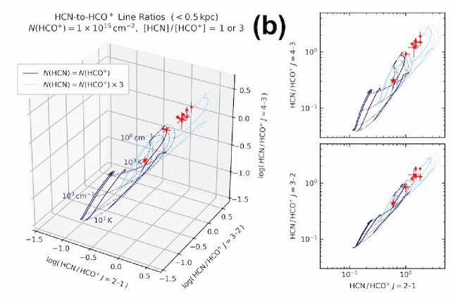
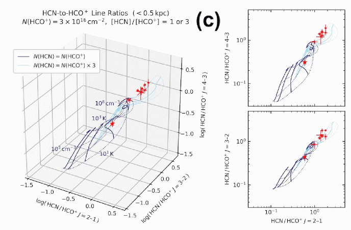
Figure 27: Same as Figure 9, but (a) HCN-to-HCO⁺ abundance ratio of [HCN]/[HCO⁺] = 1 and 7, (b) HCO⁺ column density of N_HCO+ = 1 $\times$ 10¹⁵ cm^-2 (a factor of 10 smaller than that adopted in Figure 9), and (c) N_HCO+ = 3 $\times$ 10¹⁶ cm^-2 (a factor of 3 larger). Red filled circles are the observed HCN-to-HCO⁺ flux ratios of the same (U)LIRGs as plotted in Figure 9.

Appendix H Derived Molecular Gas Density and Temperature in the Central $\lesssim$1 kpc and $\lesssim$2 kpc Regions

Figures 28 and 29 display our fitting results for molecular gas density and temperature based on the emission line flux ratios extracted from the 1 kpc and 2 kpc beam-sized spectra, respectively, using the Levenberg-Marquardt method. Table 14 summarizes these results. For (U)LIRGs for which we adopt the second fitting results (i.e., flux scaling on) for the 0.5 kpc beam-sized data (Figure 10), we do for the 1 kpc and 2 kpc beam-sized data as well, for consistent comparison of molecular gas properties among different regions of each (U)LIRG. We provide these fitting results for the 1–2 kpc beam-sized data because Imanishi et al. (2023) apply the same fitting to different nearby ULIRGs observed with comparable 1–2 kpc beam sizes. The presence of dense ($\gtrsim$10⁵ cm^-3) and warm ($\gtrsim$300 K) molecular gas in all the observed ULIRGs’ nuclei in this paper is confirmed with the 1–2 kpc beam sizes, as previously seen for different nearby ULIRGs (Imanishi et al., 2023). The derived molecular gas density ($\sim$10⁴ cm^-3) and temperature ($\sim$100 K) in the only one LIRG NGC 1614 (Figure 28h) are substantially smaller than those of the observed ULIRGs in this paper (Figure 28a–g), which also conforms to the result reported by Imanishi et al. (2023) for NGC 1614 and different nearby ULIRGs.

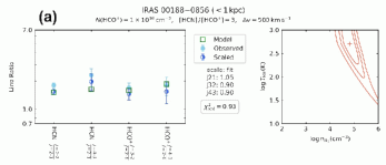
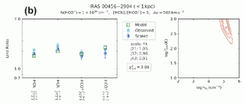
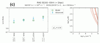
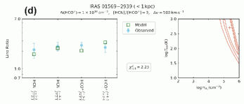
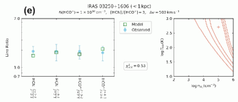
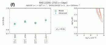
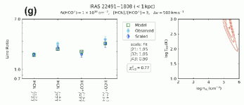
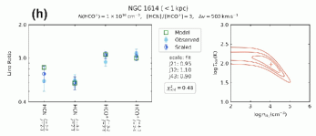
Figure 28: Fitting results for the high-J to low-J emission line flux ratios of HCN and HCO⁺ derived from the 1 kpc beam-sized spectra, displayed in the same way as Figure 10. The result of IRAS 16090$-$0139 is shown in Figure 11d.

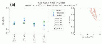
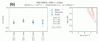
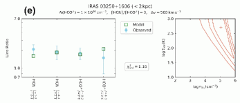
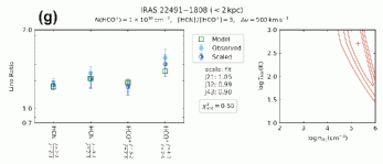
Figure 29: Same as Figure 28, but for the 2 kpc beam-sized spectra. The result of IRAS 16090$-$0139 is shown in Figure 11e. The LIRG NGC 1614 is not shown, for the same reason as explained in Figure 2 caption.

Table 14: Summary of the Best Fit Values for the 1 kpc and 2 kpc Beam-sized Data

Object	Region	Scaling	log n${}_{\rm H_{2}}$	log Tkin	Reduced
			[cm-3]	[K]	$\chi^{2}$
(1)	(2)	(3)	(4)	(5)	(6)
IRAS 00188$-$0856	$<$1 kpc	on	4.8${}^{+0.2}_{-0.2}$	2.7${}^{+\infty}_{-0.3}$	0.93
	$<$2 kpc	on	5.0${}^{+0.2}_{-0.2}$	2.7${}^{+0.4}_{-0.1}$	3.1
IRAS 00456$-$2904	$<$1 kpc	on	5.2${}^{+0.1}_{-0.2}$	2.7${}^{+0.3}_{-0.1}$	3.1
	$<$2 kpc	on	5.0${}^{+0.2}_{-0.2}$	2.7${}^{+\infty}_{-0.2}$	1.2
IRAS 01166$-$0844	$<$1 kpc	off	5.6${}^{+0.3}_{-0.4}$	2.5${}^{+\infty}_{-0.5}$	1.4
	$<$2 kpc	off	5.1${}^{+0.6}_{-0.5}$	2.7${}^{+\infty}_{-0.7}$	0.64
IRAS 01569$-$2939	$<$1 kpc	off	5.4${}^{+0.3}_{-0.2}$	2.7${}^{+\infty}_{-0.5}$	2.3
	$<$2 kpc	off	5.5${}^{+\infty}_{-0.4}$	2.5${}^{+\infty}_{-0.8}$	1.9
IRAS 03250$+$1606	$<$1 kpc	off	5.0${}^{+0.5}_{-0.4}$	2.7${}^{+\infty}_{-0.7}$	0.53
	$<$2 kpc	off	5.0${}^{+0.4}_{-0.4}$	2.7${}^{+\infty}_{-0.5}$	1.2
IRAS 22206$-$2715	$<$1 kpc	off	5.2${}^{+0.2}_{-0.2}$	2.7${}^{+\infty}_{-0.2}$	0.41
	$<$2 kpc	off	5.3${}^{+\infty}_{-0.2}$	3.0${}^{+\infty}_{-1.2}$	0.21
IRAS 22491$-$1808	$<$1 kpc	on	5.4${}^{+0.1}_{-0.2}$	2.7${}^{+0.6}_{-0.2}$	0.77
	$<$2 kpc	on	5.3${}^{+0.4}_{-0.3}$	2.7${}^{+\infty}_{-0.5}$	0.50
NGC 1614	$<$1 kpc	on	4.0${}^{+0.3}_{-0.4}$	2.0${}^{+0.1}_{-0.1}$	0.48

Note. — Col.(1): Object name. Col.(2): Region. Col.(3): Scaling on or off. Col.(4): Decimal logarithm of H₂ gas density in units of cm^-3. Col.(5): Decimal logarithm of gas kinetic temperature in units of K. Col.(6): Reduced $\chi^{2}$ value. The HCO⁺ column density, HCN-to-HCO⁺ abundance ratio, and molecular line width are fixed at N${}_{\rm HCO^{+}}$ = 1 $\times$ 10¹⁶ cm^-2, [HCN]/[HCO⁺] = 3, and $\Delta$v = 500 km s^-1, respectively.

References

- Aalto et al. (2015a) Aalto, S., Garcia-Burillo, S., Muller, S., et al. 2015a, A&A, 574, A85
- Aalto et al. (2015b) Aalto, S., Martin, S., Costagliola, F., et al. 2015b, A&A, 584, A42
- Aalto et al. (2007) Aalto, S., Spaans, M., Wiedner, M. C., et al. 2007, A&A, 464, 193
- Aladro et al. (2011) Aladro, R., Martin, S., Martin-Pintado, J., et al. 2011, A&A, 535, 84
- Aladro et al. (2015) Aladro, R., Martin, S., Riquelme, D., et al. 2015, A&A, 579, A101
- Astropy Collaboration et al. (2022) Astropy Collaboration, Price-Whelan, A. M., Lim, P. L., et al. 2022, ApJ, 935, 167
- Baan et al. (2008) Baan, W. A., Henkel, C., Loenen, A. F., Baudry, A., & Wiklind, T., 2008, A&A, 477, 747
- Baba et al. (2018) Baba, S., Nakagawa, T., Isobe, N., & Shirahata, M. 2018, ApJ, 852, 83
- Bernard-Salas et al. (2009) Bernard-Salas, J., Spoon, H. W. W., Charmandaris, V., et al. 2009, ApJS, 184, 230
- Brandl et al. (2006) Brandl, B. R., Bernard-Salas, J., Spoon, H. W. W., et al. 2006, ApJ, 653, 1129
- Butterworth et al. (2022) Butterworth, J., Holdship, J., Viti, S., & Garcia-Burillo, S., et al. 2022, A&A, 667, A131
- Clements et al. (2018) Clements, D. L., Pearson, C., Farrah, D., et al. 2018, MNRAS, 475, 2097
- Costagliola et al. (2011) Costagliola, F., Aalto, S., Rodriguez, M. I., et al. 2011, A&A, 528, 30
- Diaz-Santos et al. (2010) Diaz-Santos, T., Charmandaris, V., Armus, L., et al. 2010, ApJ, 723, 993
- Esposito et al. (2022) Esposito, F., Vallini, L., Pozzi, F., et al. 2022, MNRAS, 512, 686
- Falstad et al. (2021) Falstad, N., Aalto, S., Konig, S., et al. 2021, A&A, 649, A105
- Falstad et al. (2019) Falstad, N., Hallqvist, F., Aalto, S., et al. 2019, A&A, 623, A29
- Foreman-Mackey (2016) Foreman-Mackey, D. 2016, The Journal of Open Source Software, 1, 24
- Foreman-Mackey et al. (2013) Foreman-Mackey, D., Hogg, D. W., Lang, D., & Goodman, J., 2013, PASP, 125, 306
- Gao & Solomon (2004) Gao, Y., & Solomon, P. M. 2004, ApJS, 152, 63
- Gracia-Carpio et al. (2008) Gracia-Carpio, J., Garcia-Burillo, S., Planesas, P., Fuente, A., & Usero, A. 2008, A&A, 479, 703
- Greve et al. (2009) Greve, T. R., Papadopoulos, P. P., Gao, Y., & Radford, S. J. E. 2009, ApJ, 692, 1432
- Hailey-Dunsheath et al. (2012) Hailey-Dunsheath, S., Sturm, E., Fischer, J., et al. 2012, ApJ, 755, 57
- Harada et al. (2013) Harada, N., Thompson, T. A., & Herbst, E. 2013, ApJ, 765, 108
- Harris et al. (2020) Harris, C. R., Millman, K. J., van der Walt, S., et al. 2020, Nature, 585, 357
- Hildebrand (1983) Hildebrand, R. H. 1983, QJRAS, 24, 267
- Hunter (2007) Hunter, J. D. 2007, Computing in Science and Engineering, 9, 90
- Imanishi et al. (2023) Imanishi, M., Baba, S., Nakanishi, K., & Izumi, T. 2023, ApJ, 950, 75
- Imanishi et al. (2006a) Imanishi, M., Dudley, C. C., & Maloney, P. R. 2006a, ApJ, 637, 114
- Imanishi et al. (2007a) Imanishi, M., Dudley, C. C., Maiolino, R., et al. 2007a, ApJS, 171, 72
- Imanishi et al. (2021) Imanishi, M., Hagiwara, Y., Horiuchi, S., Izumi, T., & Nakanishi, K. 2021, MNRAS, 502, L79
- Imanishi et al. (2011) Imanishi, M., Imase, K., Oi, N., & Ichikawa, K. 2011, AJ, 141, 156
- Imanishi et al. (2008) Imanishi, M., Nakagawa, T., Ohyama, Y., et al. 2008, PASJ, 60, S489
- Imanishi et al. (2010b) Imanishi, M., Nakagawa, T., Shirahata, M., Ohyama, Y., & Onaka, T. 2010b, ApJ, 721, 1233
- Imanishi & Nakanishi (2013a) Imanishi, M., & Nakanishi, K. 2013a, AJ, 146, 47
- Imanishi & Nakanishi (2013b) Imanishi, M., & Nakanishi, K. 2013b, AJ, 146, 91
- Imanishi & Nakanishi (2014) Imanishi, M., & Nakanishi, K. 2014, AJ, 148, 9
- Imanishi et al. (2016a) Imanishi, M., Nakanishi, K., & Izumi, T. 2016a, ApJ, 825, 44
- Imanishi et al. (2016b) Imanishi, M., Nakanishi, K., & Izumi, T. 2016b, AJ, 152, 218
- Imanishi et al. (2018) Imanishi, M., Nakanishi, K., & Izumi, T. 2018, ApJ, 856, 143
- Imanishi et al. (2019) Imanishi, M., Nakanishi, K., & Izumi, T. 2019, ApJS, 241, 19
- Imanishi et al. (2022) Imanishi, M., Nakanishi, K., Izumi, T., & Baba, S. 2022, ApJ, 926, 159
- Imanishi et al. (2006b) Imanishi, M., Nakanishi, K., & Kohno, K. 2006b, AJ, 131, 2888
- Imanishi et al. (2007b) Imanishi, M., Nakanishi, K., Tamura, Y., Oi, N., & Kohno, K. 2007b, AJ, 134, 2366
- Imanishi et al. (2009a) Imanishi, M., Nakanishi, K., Tamura, Y., & Peng, C. -H. 2009a, AJ, 137, 3581
- Imanishi et al. (2020) Imanishi, M., Nguyen, D. D., Wada, K., et al. 2020, ApJ, 902, 99
- Israel (2023) Israel, F. P. 2023, A&A, 671, A59
- Izumi et al. (2016) Izumi, T., Kohno, K., Aalto, S., et al. 2016, ApJ, 818, 42
- Kamenetzky et al. (2016) Kamenetzky, J., Rangwala, N., Glenn, J., et al. 2016, ApJ, 829, 93
- Kameno et al. (2020) Kameno, S., Sawada-Satoh, S., Impellizzeri, C. M. V., et al. 2020, ApJ, 895, 73
- Kim & Sanders (1998) Kim, D. -C., & Sanders, D. B. 1998, ApJS, 119, 41
- Kluyver et al. (2016) Kluyver, T., Ragan-Kelley, B., Perez, F., et al. 2016, in Positioning and Power in Academic Publishing: Players, Agents and Agendas (IOS Press), 87–90
- Krips et al. (2008) Krips, M., Neri, R., Garcia-Burillo, S., et al. 2008, ApJ, 677, 262
- Lindberg et al. (2011) Lindberg, J. E., Aalto, S., Costagliola, F., et al. 2011, A&A, 527, A150
- Lu et al. (2017) Lu, N., Zhao, Y., Diaz-Santos, T., et al. 2017, ApJS, 230, 1
- Manohar & Scoville (2017) Manohar, S, & Scoville, N. 2017, ApJ, 835, 127
- Martin et al. (2016) Martin, S., Aalto, S., Sakamoto, K., et al. 2016, A&A, 590, A25
- Martin et al. (2011) Martin, S., Krips, M., Martin-Pintado, J., et al. 2011, A&A, 527, A36
- Martin et al. (2006) Martin, S., Mauersberger, R., Martin-Pintado, J., et al.
- Mashian et al. (2015) Mashian, N., Sturm, E., Sternberg, A., et al. 2015, ApJ, 802, 81
- Meier et al. (2011) Meier, D. S., Turner, J. L., & Schinnerer, E. 2011, AJ, 142, 32
- Meijerink et al. (2013) Meijerink, R., Kristensen, L. E., Weiss, A., et al. 2013, ApJ, 762, L16
- Meijerink et al. (2007) Meijerink, R., Spaans, M., & Israel, F. P. 2007, A&A, 461, 793
- Nakajima et al. (2018) Nakajima, T., Takano, S., Kohno, K., Harada, N., & Herbst, E. 2018, PASJ, 70, 7
- Nakajima et al. (2023) Nakajima, T., Takano, S., Tosaki, T., et al. 2023, ApJ, in press (asXiv:2307.02320)
- Nardini et al. (2010) Nardini, E., Risaliti, G., Watabe, Y., Salvati, M., & Sani, E. 2010, MNRAS, 405, 2505
- Newville et al. (2021) Newville, M., Otten, R., Nelson, A., et al. 2021, lmfit/lmfit-py: 1.0.3, Zenodo, Zenodo
- Papadopoulos et al. (2014) Papadopoulos, P. P., Zhang, Z-Y., Xilouris, E. M., et al. 2014, ApJ, 788, 153
- Pellegrini et al. (2013) Pellegrini, E. W., Smith, J. D., Wolfire, M. G., et al. 2013, ApJ, 779, L19
- Pereira-Santaella et al. (2021) Pereira-Santaella, M., Colina, L., Garcia-Burillo, S., et al. 2021, A&A, 651, A42
- Pereira-Santaella et al. (2014) Pereira-Santaella, M., Spinoglio, L., van der Werf, P. P., et al. 2014, A&A, 566, A49
- Pereira-Santaella et al. (2015) Pereira-Santaella, M., Colina, L., Alonso-Herrero, A., et al. 2015, MNRAS, 454, 3679
- Perez & Granger (2007) Perez, F., & Granger, B. E. 2007, Computing in Science and Engineering, 9. 21
- Privon et al. (2015) Privon, G. C., Herrero-Illana, R., Evans, A. S., et al. 2015, ApJ, 814, 39
- Reback et al. (2022) Reback, J., jbrockmendel, McKinney, W., et al. 2022, pandas-dev/pandas: Pandas 1.4.2, v1.4.2, Zenodo, Zenodo
- Rosenberg et al. (2015) Rosenberg, M. J. F., van der Werf, P. P., Aalto, S., et al. 2015, ApJ, 801, 72
- Saito et al. (2018) Saito, T., Iono, D., Espada, D., et al. 2018, ApJ, 863, 129
- Sakamoto et al. (2021) Sakamoto, K., Martin, S., Wilner, D. J., et al. 2021, ApJ, 923, 240
- Sanders et al. (2003) Sanders, D. B., Mazzarella, J. M., Kim, D. -C., Surace, J. A., & Soifer, B. T. 2003, ApJ, 126, 1607
- Sanders & Mirabel (1996) Sanders, D. B., & Mirabel, I. F. 1996, ARA&A, 34, 749
- Scoville et al. (2015) Scoville, N., Sheth, K., Walter, F., et al. 2015, ApJ, 800, 70
- Shirley (2015) Shirley, Y. L. 2015, PASP, 127, 299
- Sliwa & Downes (2017) Sliwa, K., & Downes, D. 2017, A&A, 604, A2
- Soifer et al. (2000) Soifer, B. T., Neugebauer, G., Matthews, K., et al. 2000, AJ, 119, 509
- Soifer et al. (2001) Soifer, B. T., Neugebauer, G., Matthews, K., et al. 2001, AJ, 122, 1213
- Spaans & Meijerink (2008) Spaans, M., & Meijerink, R. 2008, ApJ, 678, L5
- Spinoglio et al. (2012) Spinoglio, L., Pereira-Santaella, M., Busquet, G., 2012, ApJ, 758, 108
- Takano et al. (2019) Takano, S., Nakajima, T., & Kohno, K. 2019, PASJ, 71, S20
- The CASA Team (2022) The CASA Team, et al. 2022, PASP, 134, 114501
- Tunnard et al. (2015) Tunnard, R., Greve, T. R., Garcia-Burillo, S., et al. 2015, ApJ, 800, 25
- Ueda et al. (2021) Ueda, J., Iono, D., Yun, M. S., et al. 2021, ApJS, 257, 57
- van der Tak et al. (2007) van der Tak, F. F. S., Black, J. H., Schoier, F. L., Jansen, D. J., & van Dishoeck, E. F. 2007, A&A, 468, 627
- van der Werf et al. (2010) van der Werf, P. P., Isaak, K. G., Meijerink, R., et al. 2010, A&A, 518, L42
- Veilleux et al. (1999) Veilleux, S., Kim, D. -C., & Sanders, D. B. 1999, ApJ, 522, 113
- Veilleux et al. (1995) Veilleux, S., Kim, D. -C., Sanders, D. B., Mazzarella, J. M., & Soifer, B. T. 1995, ApJS, 98, 171
- Veilleux et al. (2009) Veilleux, S., Rupke, D. S. N., Kim, D.-C., et al. 2009, ApJS, 182, 628
- Virtanen et al. (2020) Virtanen, P., Gommers, R., Oliphant, T. E., 2020, Nature Methods, 17, 261
- Yuan et al. (2010) Yuan, T. -T., Kewley, L. J., Sanders, D. B. 2010, ApJ, 709, 884
- Zhou et al. (2022) Zhou, J., Zhang, Z-Y., Gao, Y., et al. 2022, ApJ, 936, 58