A study of the measurement of the lepton anomalous magnetic moment in high energy lead-lead collisions at LHC
Abstract
The lepton anomalous magnetic moment: was measured, so far, with a precision of only several percents despite its highly sensitivity to physics beyond the Standard Model such as compositeness or Supersymmetry. A new study is presented to improve the sensitivity of the measurement with photon-photon interactions from ultra-peripheral lead-lead collisions at LHC. The theoretical approach used in this work is based on an effective Lagrangian and on a photon flux implemented in the MadGraph5 Monte Carlo simulation. Using a multivariate analysis to discriminate the signal from the background processes, a sensitivity to the anomalous magnetic moment = 0 is obtained at 95% CL with a dataset corresponding to an integrated luminosity of 2 nb-1 of lead-lead collisions and assuming a conservative 10% systematic uncertainty. The present results are compared with previous calculations and available measurements.
1 Introduction
The anomalous magnetic moment of elementary particles (leptons and quarks) is defined as: where, Dirac theory of the QED implies at the classical level, . The measurement of is today one of most powerful tool to test the validity of the the Standard Model (SM) theory that, despite its indisputable success, can not be a complete theory. There are, in fact, several unresolved questions not addressed by the SM such as, for example, the existence of “dark matter”, estimated to be about 5 times more abundant than the ordinary matter. Precise measurements of the elementary particles magnetic moment and its comparison with the Standard Model predictions could indicate the existence of new interactions and particles that could shed light also on the nature of the dark matter and on the problems of the naturalness and fine tuning of the Higgs boson mass.
Extensive researches of new physics, new particles, deviations from the SM predictions, have been carried out at the LHC, but no clear hints of the existence of new phenomena have emerged from the data collected so far. The LHC run has re-started in 2022 with the LHC performances improved both in energy and luminosity and searches of new particles will continue, but the limited energy/mass at which they could be produced and detected will remain to be of the order of 1 TeV.
A discrepancy between the values of predicted by the SM and the measured ones could provide important clues to anticipate both the nature and the mass of the new phenomena suggesting also the energy regime at which a direct production of the new particles responsible of these discrepancies could be expected. This, of course, would be possible, if, in one hand, a precise calculation is provided of the SM predictions, and, on the other hand, accurate measurements of the the anomalous will be performed for the three charged leptons.
For an accurate prediction of within the SM it is crucial a precise evaluation of high order electromagnetic (QED), weak and strong (QCD) interactions corrections. These QED corrections were first calculated, for the electron, in the seminal paper by J. Schwinger [1] to be , where is the fine structure constant.
The QCD corrections are difficult to calculate in an energy range where no perturbation development is applicable and corrections should rely on experimental cross sections in lepton-hadron and hadronic interactions with the help of the dispersion relation techniques. The size of the hadronic corrections strongly depends on the mass of the lepton under study becoming more and more relevant as the the lepton mass increases.
The experimental technique to measure : , is different for the three charged leptons. An extreme precision of ppb for is obtained by a single-electron quantum cyclotron frequency measurements [2]. A recent improved observation of the fine structure constant led to a difference between the measured and predicted negative and significant at 2.4 ’s [2].
For the muon, is measured by comparing the cyclotron and the muon magnetic moment precession frequencies. The recent experiment at Fermilab, ‘”Muon g-2”, measured with a precision of 0.46 ppm [3]. The difference between the SM prediction of , with hadronic contributions calculated via the dispersion relation method [4], and the combined“Muon g-2” and E821 at BNL experiments, shows a discrepancy of 4.2 . However, a new estimate of the theoretical predicted value of obtained by recalculating the hadronic contributions using a lattice QCD approach, resulted into a theoretical prediction compatible with the experimental value within 1.2 [5].
The theoretical prediction of , although not as precise as those ones for lighter leptons, is by far more accurate than the experimental measurements. Theoretically, the larger mass makes the hadronic contributions much larger than in case of the electron and the muon and, consequently, also the uncertainties of the is much larger. Possible contributions to given from new particles of mass to the photon-lepton vertex are expected to be of the order of for a lepton of mass . Therefore, new physics effects for the would be enhanced by a factor = 286 with respect to . Moreover, in some models addressing recent anomalies in [6], a significant contribution to could arise from new scalar and tensor operators and could be as large as [7].
The would also be sensitive to possible lepton compositeness that, in general, would contribute with corrections , where is the ”compositeness” scale [8], possibly generated by warped extra-dimensions [9, 10, 13, 11, 12].
The investigation, definitely, represents an excellent tool to access new physics beyond the SM (BSM).
Unfortunately the present experimental knowledge of is poor. In fact the very short -lifetime precludes the use of the precession frequency measurement method as done in the case. The method adopted is to exploit the sensitivity to of the total and differential cross-sections, in photon-photon scattering111The first idea of using photons accompanying fast moving charged particles for physics experiments is due to Enrico Fermi in 1924 [14]. . The best measurement at LEP was obtained by the DELPHI experiment [15] and provided the limit at CL. The combined reanalysis of various experimental measurements such as the cross section, the transverse polarization and asymmetry, as well as the decay width , allowed the authors in [17] to set a stronger, but indirect, model-independent limits on new physics contributions to : . Other strategies to measure the anomalous moment at the LHC have been proposed in [18], by considering the rare Higgs decay , which shows a sensitivity at the percent level and the measurement of the distribution of the large transverse mass of produced in proton-proton collisions [16].
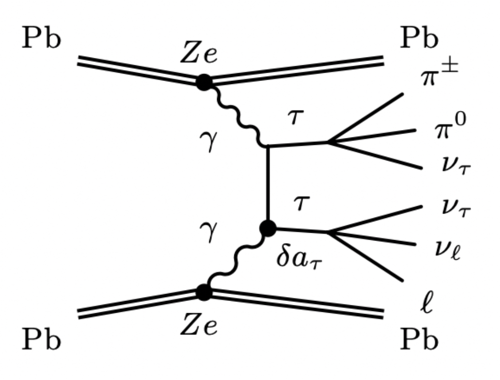
Recent papers proposed to use ultraperipheral collisions of heavy ions at LHC to measure the exclusive production cross section [19] [20]. Using Pb-Pb ultraperipheral collisions to single-out collisions yielding , offers several advantages compared with proton-proton collisions at LHC. In fact, in Pb-Pb collisions the cross section for (see Figure 1) is enhanced by a factor , largely compensating the lower integrated luminosity compared with that available in proton-proton collisions. In addition, the request of an exclusive final state containing only tau-decay products, with essentially no pile-up background, allows a better control of the background processes than in case of p-p collisions.
At LHC the measurements have been obtained with Pb-Pb collisions by the ATLAS and CMS experiments. CMS, with an integrated luminosity of obtained the limit of at 68% CL [21]. ATLAS, using an integrated luminosity of 1.44 provided a limit of at 95% CL [22]. These measurements at LHC have still an uncertainty of several percents dominated by the statistical error. This uncertainty is expected to be reduced by about one order of magnitude with the new data to be collected at HL-LHC with an increased integrated luminosity of a factor 10.
A measurement of is proposed to be performed also at the new -factories such as the collider Belle2 [23]. It has been estimated that with 50 the Belle-II experiment could set the limit (1.5% of the SM prediction). Still at Belle-II with an integrated luminosity of 40 and using polarised electron beams a precision on of could be achieved [24]. However no systematic uncertainty was taken into account, and the detector response was described by a fast simulation.
The theoretical prediction is: [25] where the largest contribution to the uncertainty is due to hadronic effects. By comparing the present with it is clear that the sensitivity of the existing measurements is still more than one order of magnitude worse than needed.
The discrepancies between experiment and theory already observed for both and makes the exploration of the tau lepton magnetic moment even more crucial for fundamental physics and more efforts should be devoted especially in refining the experimental methods to measure it.
The growing interest around the rich physic program provided by photon interactions generated by heavy ions at LHC has also fostered the development of tools to improve the generation of these type of events. It is important to identify tools for event generation that provide a good compromise between flexibility and precision. For this reason in this work the signal production is generated with an effective description in a UFO model (Universal FeynRules Output) [26] implemented in the Monte Carlo generator MadGraph5 [27]. This choice provides several advantages compared with previous approaches [20] allowing to distinguish the linear interference between SM and BSM and the pure quadratic BSM contribution. Moreover, an easier and more effective interface among the particle level simulation, the showering/hadronization and the detector effects is possible. Details on the adopted model will be given in the following chapter. The detector performance and the experimental environment at LHC are those of the ATLAS experiment.
In this work the analysis of data to extract is performed by exploiting a Gradient Boosted Decision Trees (BDTG) [28] approach that optimises the signal selection together with the best background rejection. To verify the performance of this new approach the results achieved with the BDTG analysis are compared with those obtained with a Standard Cuts (SC) mimicking that one applied in previous LHC experiments. Results refer to an integrated luminosity of 2.0 corresponding to the total integrated luminosity of the 2015-2018 heavy ions data-taking. In addition, results for 1.44 of integrated luminosity are also quoted to have a direct comparison with the latest published ATLAS results [22].
2 Generation of signal and background processes
In this section the steps to generate and simulate signal and background processes are discussed. The photon flux implementation and the advantage of using Pb-Pb with respect to proton-proton collisions are discussed in section 2.1 . The signal process generation, including the contribution from BSM effects is described in section 2.2. In this section is also discussed the effect on differential and total cross-sections due to a modified value of . The background processes relevant to this study are presented in section 2.3. Detector effects have been simulated with a fast simulation as described in section 2.4.
2.1 The photon flux
In this work the process is generated by modifying MadGraph5 to include the photon flux from the lead beams in ultra-peripheral collisions following the prescription in reference [29]. In the Equivalent Photon Approximation (EPA) [30, 31], and neglecting non-factorizable hadronic interactions between nuclei and nuclear overlap effects, the cross section in ultra-peripheral Pb-Pb collisions can be expressed as the convolution:
| (1) |
where is the elementary cross-section and represents the photon flux from the two Pb-ions, calculated as a function of the ratio of the emitted photon energy from the ion with the beam energy (). is described by the classical analytic form [32]:
| (2) | ||||
where, for Pb, , , the nucleon mass GeV, the nucleus radius GeV fm, is the minimum impact parameter and are the modified Bessel functions of the second kind of the first (second) order. The same implementation of the photon flux is also used in [19], where it is found that a more complete treatment of nuclear effects, as included in program as SUPERCHIC [33], do not impact significantly the cross sections and distributions of the processes which are relevant for our study.
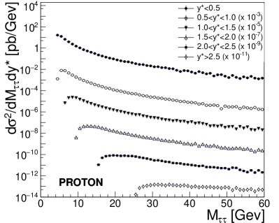
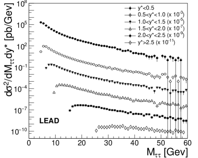
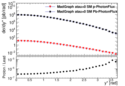
A comparison between the di-tau double differential cross section from proton-proton and from lead-lead collisions is shown in Figure 2. The proton distributions are obtained using MadGraph5 default configuration, which adopts the EPA improved Weizsaecker-Williams formula [34]. The figures show the double-differential di-tau cross sections as a function of the di-tau mass in bins of half the rapidity separation, (), of the 2 taus.
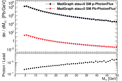
The comparison between lead and proton cross sections and their ratio as a function of di-tau mass and of the di-tau rapidity integrated on the di-tau separation and di-tau mass respectively, are shown in Figure 3. It is interesting to note that the expected enhancement in favour of the radiation intensity from Pb reduces as di-tau mass or rapidity separation increases. In fact, as the di-tau mass (or the di-tau separation) increases, also the of the interaction increases, and the interaction radius decreases accordingly. In this situation, the electromagnetic form factor generated by the lead nucleus decreases its effectiveness in photon emission. This effect is encoded in the photon flux dependence on of the analytic form in Eq. (2), which is based on classical electrodynamics.
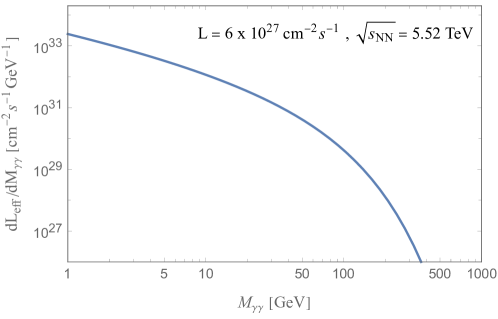
The cross section in Eq. (1) can be also expressed in terms of an effective luminosity () as:
| (3) |
Figure 4 shows the effective luminosity, as a function of the photon-fusion mass , as obtained from the convolution of the photon flux in (1).
2.2 Generation and simulation of the signal
Events including BSM physics through a modified value of are generated implementing in a UFO model [35], to be used in MadGraph5, the effective Lagrangian term:
| (4) |
by means of Feynrules [36]. The implementation is validated against theoretical analytical predictions and previous results from LEP [15].
The approach to generate BSM effects here described differs from previous analysis. In fact, the authors in [20] use a custom code, which generates the signal by means of the full form of the photon-tau vertex function and of the cross sections calculated at leading order. The MadGraph5 approach, implementing the signal generation via an effective description in a UFO model, allows an easier interface with showering/hadronization effects and with the detector simulation. Moreover, it also allows to easily single-out the linear interference terms with the SM from the purely BSM quadratic terms. The SM and BSM inclusive cross sections here obtained show an agreement within 10% with those in [20].
The study in [19] adopts our same implementation of the photon flux in MadGraph5, as also MadGraph5 for signal simulations. However, [19] makes use of a different UFO model, the SMEFTsim package [37], and extracts the BSM modification to from the parameters of the SM effective field theory considered in this SMEFTsim code.
A significant discrepancy is observed between the BSM signal cross section values of [19] and the calculation here presented; on the contrary the two SM results are in agreement. Since the two BSM calculations rely on an EFT approach, the source of the disagreement it is most probably not connected to the EFT but to an issue occurred in [19] with the conversion between SMEFTsim operators and those generating modification to . A similar discrepancy is observed between the results in [19] and the BSM cross section calculations reported in [20].
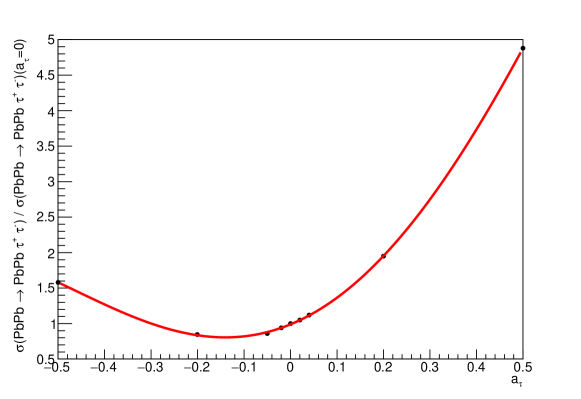
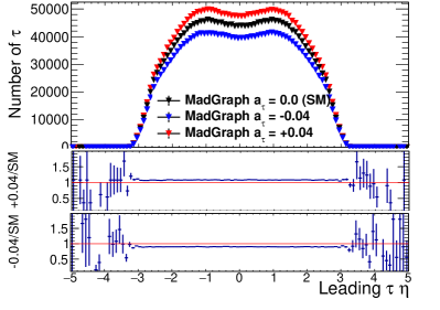
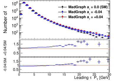
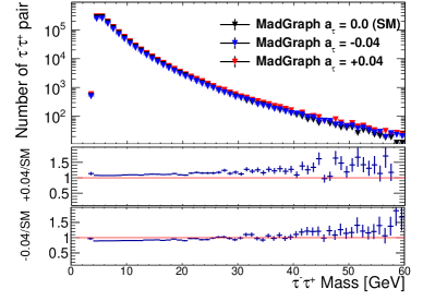
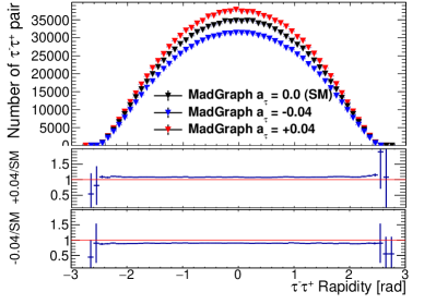
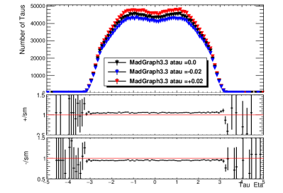
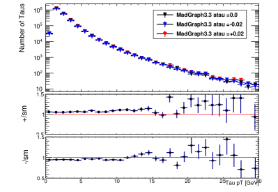
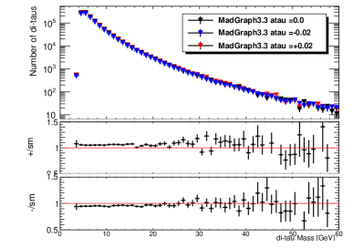
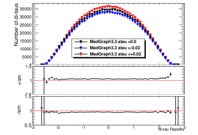
The ratio between the total cross section and the SM cross section as a function of is shown in Figure 5, where the ratio is set to 1 for , considered as the SM value. The asymmetry between positive and negative values is due to interference between the SM part and the BSM modified coupling. The effect of different values is investigated by looking at various and di- kinematical distributions. In particular, Figure 6 shows the leading , the leading rapidity, the di-tau system rapidity and invariant mass distributions for three representative values of () normalized to of integrated luminosity. Figure 6 proves that, in addition to the -pair cross section, also the differential cross sections, especially the distribution, can be exploited to improve the sensitivity to .
2.3 Background processes
The requirement of selecting exclusive di-tau decay products in UPC events greatly reduces the background contribution in the signal selection. The background processes considered are , ,, . Among these processes the processes where one of the radiate a photon is the major source of background. As shown in [19] and [20], the produces a larger charged-particle multiplicity than the signal and hence can be totally rejected by exclusivity requirements.
Other contributions to the background could be due to diffractive photo-nuclear events, mediated by a Pomeron exchange, where the Pb-ions may not dissociate and some particles could be produced in the central rapidity region. For this background, a reliable Monte Carlo simulation is not available, however in reference [22] it was estimated, by a data-driven method, that this contribution results in a about contribution to the data sample. In this analysis this contribution has been neglected.
Two millions events of background samples have been produced with PYTHIA8, see appendix A for details.
2.4 Simulation of detector effects
The simulation of the ATLAS detector is done by using DELPHES 3.5.0 framework [39]. This package implements a fast-simulation of the detector, including a track propagation system embedded in a magnetic field, the electromagnetic and hadron calorimeter responses, and a muon identification system. Physics objects as electrons or muons are then reconstructed from the simulated detector response using dedicated sub-detector resolutions. For the analysis here presented, electron [40] and muon [41] efficiencies have been modified using the latest ATLAS performance results as obtained on the data sample collected in 2015-2018 (Table 1). Other efficiencies such as the tracking efficiency or the smearing reconstruction functions are used without changes.
3 Analysis procedure
In this section the procedure to select the signal from the background processes is described. The analysis is applied to the data including the fast detector simulation. The preselection cuts and the signal region definition are described in section 3.1. The two analysis procedures based on Standard Cuts (SC) and on a multivariate approach (BDTG) respectively are presented in section 3.2.
3.1 Preselection and signal region definition
Event selection requires at least one decayed leptonically. The second is requested to decay hadronically and is reconstructed requiring one or three tracks. Two signal regions are identified according to the decay topologies: one lepton one track (1L1T) and one lepton three tracks (1L3T) respectively. These requirements potentially collect about of all possible -pair decays, as shown in Table 2. The signal region where both the ’s decay leptonically is not included in this analysis due to the low statistics obtained after the lepton identification, see Table 11 in appendix D for more details. The final state with leptons is fundamental for the trigger selection.
| Tau Decay | Decay Process | Branching |
| Definition | Fraction | |
| Lepton Decay | 17.85% | |
| 17.36% | ||
| One Charged Pion Decay | 46.75% | |
| (n=0,1,2,3) | ||
| Three Charged Pion Decay | 13.91% | |
| (n=0,1) |
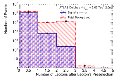
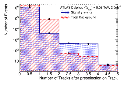
Preselection cuts, mimicking the minimal ATLAS object selection, are applied on leptons: GeV and for electrons (muons). In addition, each track is requested to satisfy minimal acceptance criteria: 500 MeV and 2.5. The preselection cuts are summarized in Table 3. The lepton and track multiplicities for signal and background processes after the preselection cuts are shown in Figure 7, the plots show that a requirement of a single lepton and one or three tracks collect most of the signal events rejecting a large fraction of the background.
| Preselection | Cuts |
|---|---|
| Electron Identification | GeV, |
| Muon Identification | GeV, |
| Track Identification | 500 MeV, 2.5 |
3.2 Signal extraction: SC and BDTG selections
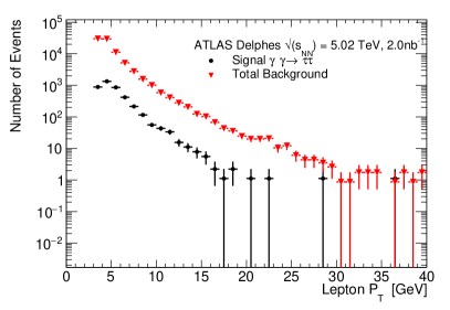
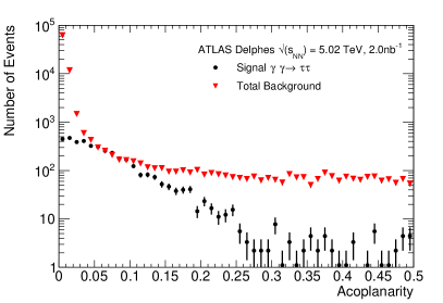
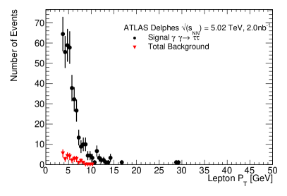
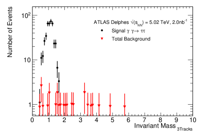
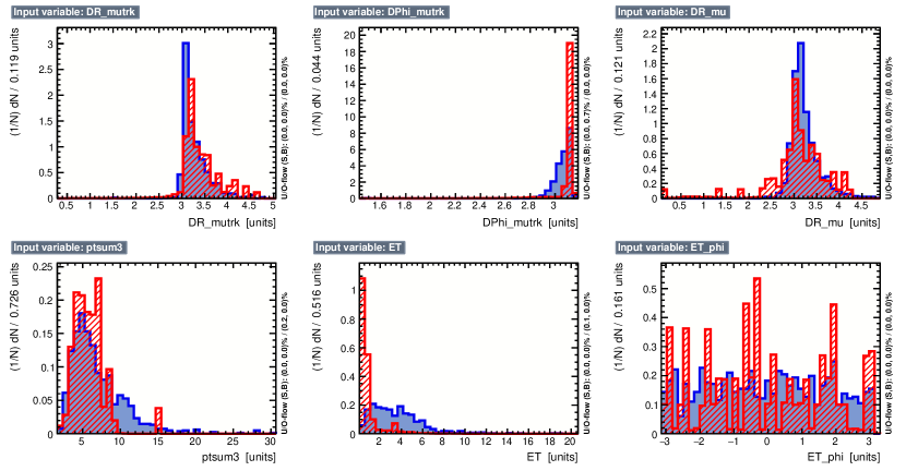
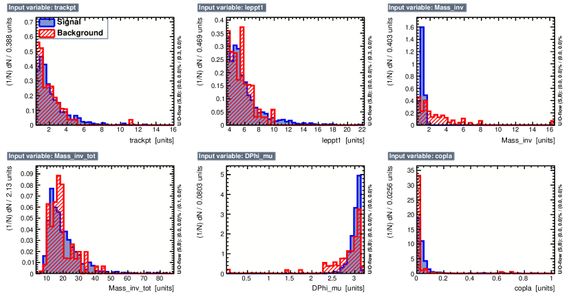
The signal and background distributions of kinematic variables of interest after the preselection cuts are shown in Figure 8 and 9 for 1L1T and 1L3T signal region respectively. These distributions include all the background processes described in section 2.3 and are normalised to 2.0 of integrated luminosity. The acoplanarity variable between the muon and the track (three tracks system) is defined as acoplanarity = , while the missing transverse energy () is calculated from calorimeter energy deposits () as . The acoplanarity and the missing transverse energy distributions for 1L1T SR show, as expected, a strong difference between signal and background due to the presence of neutrinos from tau decays. The number of simulated background events, after the preselection for 1L3T SR, is very limited, however, the invariant mass of the three non-lepton tracks (Mass3T) plot shows a significant separation between signal and backgrounds. The lepton for both signal regions do not show any significant discrimination between the signal and the background sample. The cut applied on muon is increased to 4 GeV for both the signal regions to apply the same efficiency of the electrons identification and to mimick the muon threshold used in the ATLAS trigger.
The applied kinematic selection for the SC analysis is:
-
•
1L1T:
in order to reduce the overlap with the lepton, the track must fulfill an angular requirement: 222(lepton-trk)= where and are the pseudorapidities and the azimuthal angles of the lepton and of the track, respectively.. The total charge of track plus lepton must be zero. In order to reduce the dilepton background, the lepton-track system is required to fulfill the cut: acoplanarity 0.4.
-
•
1L3T:
the three tracks are required not to overlap the lepton by applying the cut defined above on. The total charge of the three tracks plus the lepton must be zero.
The invariant mass of the three non-lepton tracks () is required to satisfy to help the identification of the lepton. The acoplanarity 0.2 requirement is also applied to reduce the lepton background.
A summary of the SC selection for 1L1T and 1L3T is shown in Table 4.
| Signal Region 1 Lepton | Signal Region 1 Lepton |
|---|---|
| and 1 Track (SR1L1T) | and 3 Track (SR1L3T) |
| 1 Lepton | 1 Lepton |
| 1 Track | 3 Tracks |
| 1.7GeV | |
| acoplanarity0.4 | acoplanarity0.2 |
| 4GeV | 4GeV |
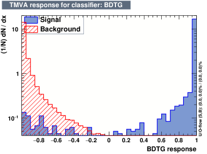
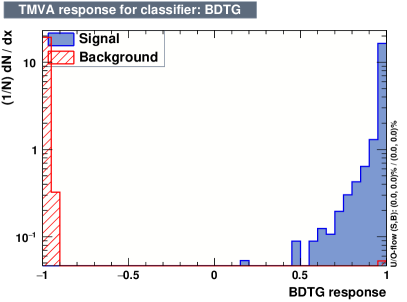
In order to investigate possible improvements in the signal over background ratio, a multivariate analysis has been implemented using gradient boosted decision tree (BDTG) in the TMVA framework [42]. The BDTG aims at improving the selection by fully exploiting the final state kinematical variables. The complete list of the variables used for the two signal regions, ordered by BDTG ranking, is reported in Table 5. The BDTG distributions are shown in Figure 10 for signal and background processes for the two signal regions. The signal selection is obtained by applying thresholds on the BDTG distributions. The two thresholds, for 1L1T and 1L3T, are obtained based on best significance criterion with significance defined as .
For 1L1T the BDTG threshold is set to BDTG 0.84 corresponding to a significance of 58 to be compared with a significance of 27 obtained with the SC analysis at 2 of integrated luminosity. For the signal region 1L3T the cut on BDTG is set to BDTG with a significance of 20 to be compared with a significance of 18 obtained with the SC analysis at 2 of integrated luminosity.
| SR 1 Lepton and 1 Track | SR 1 Lepton and 3 Tracks |
|---|---|
| SR1L1T | SR1L3T |
| Sum 3 tracks | |
| Track | Invariant Mass(Lepton+3Tracks) |
| Lepton | Lepton |
| Lepton | Invariant Mass (3Tracks) |
| Missing | R (Lepton-3tracks system) |
| Acoplanarity | (Lepton-3tracks system) |
| Track | Missing |
| Invariant Mass (Lepton+Track) | R (Lepton-Track) |
| R (Lepton-Track) | Track |
| Sum 3 tracks | (Lepton-track) |
| Lepton | Acoplanarity |
| (Lepton-track) | () |
| () |
4 Sensitivity to the tau anomalous magnetic moment
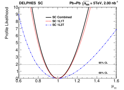
In this section the sensitivity to the signal strength , defined as the ratio of the observed signal yield to the SM expectation assuming the SM value for =1, and to the anomalous magnetic moment , are presented. Both estimates, carried out by using a profile-likelihood fit [43] on the lepton transverse momentum distributions, are obtained for the SC and the BDTG analyses.
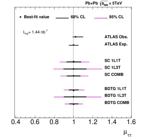
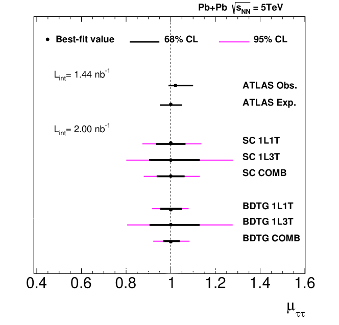
The sensitivity to the signal strength at CL 95% are measured to be and for the SC and BDTG analysis respectively. This estimates are obtained using Asimov Data. The normalization systematic uncertainties included are: the luminosity estimated to be 2% and an additional 10% to take into account the experimental conditions. These results are illustrated in the plots of Figure 11 where a clear improvement of the precision is shown with the BDTG approach. The sensitivity obtained for the two signal regions and for the two analysis selections presented in this work are compared to the ATLAS measurement in Figure 12. In this Figure 12, the integrated luminosity of the two analysis selections is scaled to 1.44 , the same integrated luminosity of the quoted ATLAS results.
| 95% CL | SR 1L1T | SR 1L3T | Combined |
|---|---|---|---|
| SC | = 1 | = 1 | = 1 |
| BDTG | = 1 | = 1 | = 1 |
| SC | = 0 | = 0 | = 0 |
| BDTG | = 0 | = 0 | = 0 |
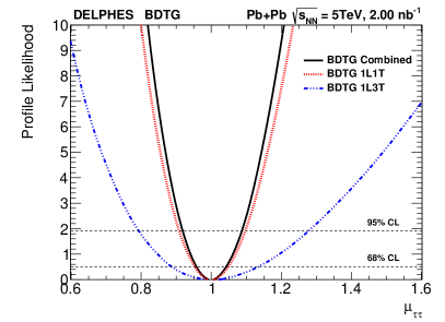
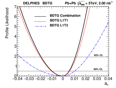
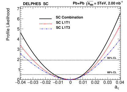
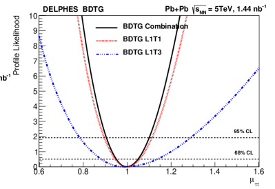
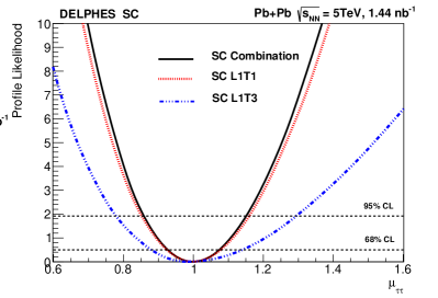
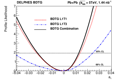
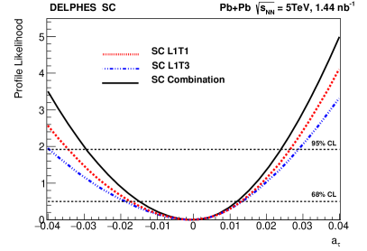
The sensitivity to is estimated with a fit where is the only free parameter and using the lepton transverse momentum distribution with a nominal value of set to the SM value (=0). Simulated signal samples with various values are included in the fit. The profile likelihood scan are presented in Figure 13. The sensitivity to at 95% CL are = and = 0 using the BDTG and SC analysis respectively. A clear improvement in the sensitivity to is shown when using the BDTG approach.
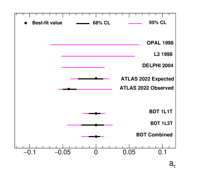
The sensitivity obtained on with the BDTG analysis is compared with previous measurements in Figure 14. The integrated luminosity of the BDTG analysis in this figure is scaled to 1.44 , the same integrated luminosity of the latest ATLAS results.

5 Conclusions
A study was presented of the ultra-peripheral process using a signal and background simulation, based on experimental conditions and detector performances of the ATLAS experiment at the CERN LHC. One is required to decay leptonically while the other one decays hadronically, into one or three tracks. This study aims at an estimation of the precision in the signal strength measurement and of the sensitivity achievable in the determination of the anomalous magnetic moment .
A different approach than in previous studies was adopted by using the signal events produced by an effective -generating Lagrangian term, implemented in the MadGraph5 Monte Carlo generator. Signal and background events were normalised at a luminosity of . The signal selection was performed with a SC procedure and with a new BDTG approach.
As a result:
-
•
the signal strength at 95% CL was achieved with the BDTG selection, to be compared with obtained with the SC procedure.
-
•
The sensitivity to at 95% CL resulted to be by using the BDTG method and = 0 by using the SC selection.
Our results show that, using the BDTG approach, a significant improvement in precision could be obtained for both and determinations compared to the latest limits published by the ATLAS experiment [22]. The present expected ATLAS sensitivity to is about 0.06 (at 95 %CL) dominated by statistics (0.045).
In this work we introduced a systematic uncertainty of 2% from LHC luminosity and an additional conservative systematic uncertainty of 10% on the overall production cross section yielding a sensitivity to of 0.03 and 0.047 for the BDT approach and the cut-flow procedure respectively, with an improvement of % in favour of BDT.
However these results look still insufficient to explore new physics. It would be desirable to obtain at least a sensitivity of in measurement, so approaching the order of magnitude expected in the SM, dominated by 1 loop contribution in QED.
In fact it is worth to note that there are new physics models predicting as large as ([7]).
We believe that with the upcoming experiments in proton-proton and heavy ions collisions at LHC and collisions at Belle2, thanks to higher collected luminosities, but also with the help of new analysis procedures, the measurements could be performed with a precision better by at least one order of magnitude than done in the past, providing a new window in search for new physics.
Acknowledgements
We thank g-2 tau ATLAS working group, in particular M. Dyndal, L. Beresford, for the useful discussion on the expected results and private communications. We thank P. Paradisi and A. Strumia for useful discussions. NV thanks G. Landini, A. Strumia and J. Wang for help in the validation of the UFO model.
Appendix A Monte Carlo distributions and Cross Sections
Several background samples have been included in this analysis, two millions events for each sample have been generated and simulated. Table 7 reports the complete list of the samples used with the production cross section and the expected number of events at 2.0 of integrated luminosity. Cuts on lepton GeV and are applied at generation level.
| Sample | Cross Section () | events@2 |
|---|---|---|
| SM () | 1111111 | |
| SM+BSM () | 1176470 | |
| SM+BSM () | 1052631 | |
| SM+BSM () | 1081081 | |
| SM+BSM () | 1142857 | |
| SM+BSM () | 998000 | |
| SM+BSM () | 1212121 | |
| 869565 | ||
| 869565 | ||
| 3257 | ||
| 6557 | ||
| 7380 |
Figure 15 shows the distributions of tau and di-tau system for the value of compared with the nominal Standard Model .
Appendix B Boosted Decision Tree
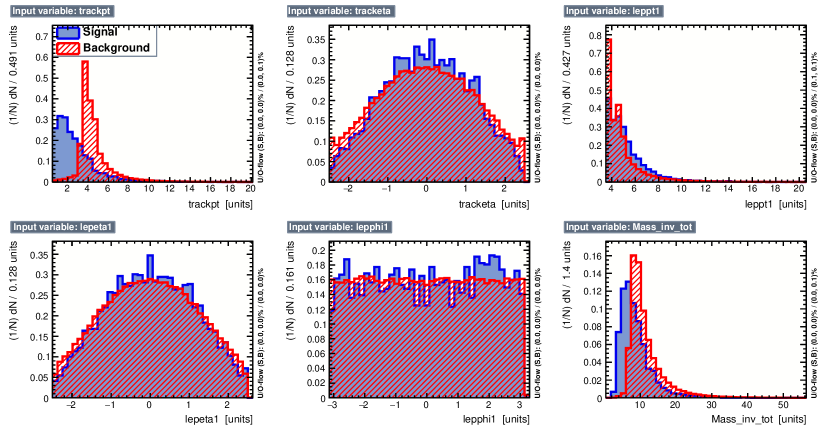
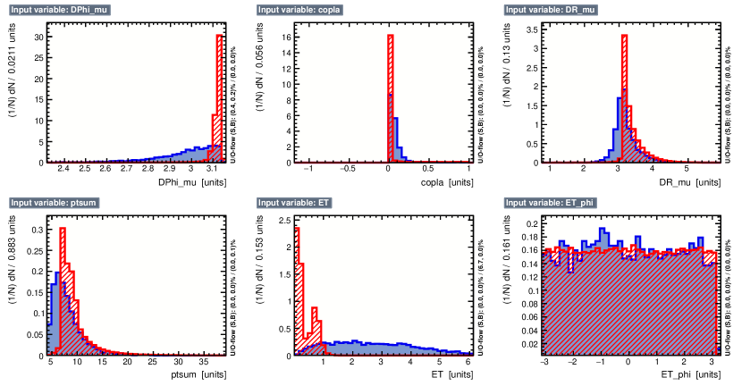
In this appendix, the BDTG observables used in the evaluation are shown for each channel. The background sample used is the sum of the background channels already shown in Table 7.
The Figure 17 and the Figure 16 report for 1L1T and 1L3T respectively the distributions of the variables used for the selection.
Appendix C Profile Likelihood at 1.44 nb-1 integrated luminosity.
In this appendix, the profile likelihoods obtained for 1.44 integrated luminosity are shown. This integrated luminosity corresponds to the integrated luminosity collected with heavy ions collisions in the year 2018 (2015 excluded).
The sensitivity to the signal strength at CL 95% are measured to be and for the SC and BDTG analysis respectively. This estimates are obtained using Asimov Data. The normalization systematic uncertainties included are: the luminosity estimated to be 2% and an additional 10% for a more realistic estimate of the experimental conditions. These results are illustrated in the plots of Figure 18 where a clear improvement of the precision is shown with the BDTG approach.
| SR 1L1T | SR 1L3T | Combined | |
|---|---|---|---|
| SC (95% CL) | = 1 | = 1 | = 1 |
| BDTG (95% CL) | = 1 | = 1 | = 1 |
| SC (95% CL) | = 0 | = 0 | = 0 |
| BDTG (95% CL) | = 0 | = 0 | = 0 |
The sensitivity to is estimated with a fit where is the only free parameter and using the lepton transverse momentum distribution with a nominal value of set to the SM value (=0). Simulated signal samples with various values are included in the fit. The profile likelihood scan are presented in Figure 19. The sensitivity to at 95% CL are = 0 and = 0 using the BDTG and SC analysis respectively. A clear improvement in the sensitivity to is shown when using the BDTG approach.
The sensitivity obtained on with the BDTG analysis and with an integrated luminosity of 2.0 is compared with previous measurements in Figure 21.
Appendix D Selection Cut Flow
In this appendix, the selection cuts applied to all the signal regions are shown. The di-lepton signal region is also included for completeness, however the low statistics preclude the test of the BDT method. Therefore, the two leptons signal region (2LSR) is also removed from the final limits comparison. The Table 10 and Table 11 report the event yields after each cut normalised to 2 of integrated luminosity for the 1L1TSR, 1L3TSR and 2LSR.
| Selection | |||||||
|---|---|---|---|---|---|---|---|
| Cuts | -0.04 | -0.02 | -0.01 | SM 0 | +0.01 | +0.02 | +0.04 |
| Total Event | 1000000 | 1052631 | 1081081 | 1111111 | 1142857 | 1176470 | 1212121 |
| Signal Region 1 Lepton and 1 Track (SR1L1T) | |||||||
| 1 Lepton | 5828.5 | 5804.41 | 5766.66 | 6075.59 | 6113.13 | 6580.31 | 7057.2 |
| 1 Track | 3917 | 3905.02 | 3923.1 | 4031.52 | 4091.79 | 4422.94 | 4804.2 |
| 3853 | 3845.06 | 3864.24 | 3967.14 | 4030.69 | 4349.44 | 4729.2 | |
| Acoplanarity0.4 | 1757.5 | 1811.02 | 1773.9 | 1893.11 | 1872.31 | 2029.78 | 2149.2 |
| 4GeV | 1320 | 1336.04 | 1318.14 | 1403.04 | 1374.4 | 1513.51 | 1596.6 |
| 1GeV | 1220.5 | 1237.15 | 1213.92 | 1283.16 | 1259.63 | 1392.97 | 1480.2 |
| Signal Region 1 Lepton and 3 Track (SR1L3T) | |||||||
| 1 Lepton | 5828.5 | 5804.41 | 5766.66 | 6075.59 | 6113.13 | 6580.31 | 7057.2 |
| 3 Tracks | 422 | 410.28 | 371.52 | 416.81 | 433.39 | 450.99 | 488.4 |
| 420.5 | 409.23 | 369.36 | 416.25 | 431.68 | 450.41 | 487.2 | |
| 1.7GeV | 420 | 403.97 | 365.58 | 413.48 | 426.54 | 449.23 | 484.8 |
| Acoplanarity0.2 | 403 | 383.98 | 345.06 | 390.72 | 403.13 | 420.42 | 459.6 |
| ¿4GeV | 344 | 327.70 | 299.7 | 323.01 | 336.32 | 355.74 | 397.8 |
| Selection | ||||||
| Total Event | 1111111 | 869565 | 869565 | 3245.91 | 6557.38 | 7380.07 |
| Signal Region 1 Lepton and 1 Track (SR1L1T) | ||||||
| 1 Lepton | 6081.06 | 57964.6 | 35241.6 | 18.96 | 0.31 | 0.03 |
| 1 Track | 4035.15 | 54400.6 | 27396.2 | 1.43 | 0.05 | 0 |
| 3970.71 | 54399.7 | 27395 | 0.88 | 0.02 | 0 | |
| Acoplanarity0.4 | 1894.81 | 1193.53 | 435.71 | 0.52 | 0.003 | 0 |
| 4GeV | 1404.3 | 746.75 | 435.71 | 0.31 | 0.003 | 0 |
| Signal Region 1 Lepton and 3 Track (SR1L3T) | ||||||
| 1 Lepton | 6081.06 | 57964.6 | 35241.6 | 18.96 | 0.31 | 0.03 |
| 3 Tracks | 417.18 | 13.62 | 5.53 | 3.82 | 0.09 | 0.09 |
| 416.63 | 13.19 | 5.53 | 1.91 | 0.05 | 0 | |
| 1.7GeV | 413.85 | 5.96 | 2.55 | 0.40 | 0.01 | 0.01 |
| Acoplanarity0.2 | 391.07 | 5.96 | 1.70 | 0.35 | 0.01 | 0.01 |
| 4GeV | 323.30 | 4.68 | 1.70 | 0.23 | 0.01 | 0.01 |
.
| Selection | ||||||
| Total Event | 1111111 | 869565 | 869565 | 3245.91 | 6557.38 | 7380.07 |
| Signal Region 2 Leptons (SR2L) | ||||||
| 1 Muon + 1 Electron | 117.77 | 0.85 | 0.85 | 0.05 | 0 | 0 |
| Charge =0 | 117.77 | 0.43 | 0.85 | 0.04 | 0 | 0 |
| GeV | 101.66 | 0.43 | 0.85 | 0.03 | 0 | 0 |
| in =0 | 101.66 | 0.43 | 0.85 | 0.03 | 0 | 0 |
References
- [1] J. Schwinger, ”On Quantum-Electrodynamics and the Magnetic Moment of the Electron”, Phys. Rev. 73, 416 – Published 15 February 1948.
- [2] D. Hanneke, S. Fogwell Hoogerheide, and G. Gabrielse, ”Cavity control of a single-electron quantum cyclotron: Measuring the electron magnetic moment” Phys. Rev. A 83, 052122 – Published 24 May 2011.
- [3] Muon g-2 collaboration, B. Abi et al., ”Measurement of the Positive Muon Anomalous Magnetic Moment to 0.46 ppm”, Phys. Rev. Lett. 126 (2021) 141801 [2104.03281].
- [4] T. Aoyama, N. Asmussen, M. Benayoun, J. Bijnens, T. Blum et al., ”The anomalous magnetic moment of the muon in the standard model”, Phys. Rep. 887, 1 (2020).
- [5] Sz. Borsanyi et al., ”Leading hadronic contribution to the muon magnetic moment from lattice QCD”. Nature volume 593, pages 51–55 .
- [6] R. Aaij et al. et al. [LHCb], Phys. Rev. Lett. 115, no.11, 111803 (2015). [erratum: Phys. Rev. Lett. 115, no.15, 159901 (2015)] doi:10.1103/PhysRevLett.115.111803 [arXiv:1506.08614 [hep-ex]].
- [7] F.Feruglio, P.Paradisi and O.Sumensari, ”Implications of scalar and tensor explanations of ”, JHEP, 191 (2018) doi:10.1007/JHEP11(2018)191.
- [8] D. J. Silverman and G. L. Shaw, ”Limits on the Composite Structure of the Tau Lepton and Quarks From Anomalous Magnetic Moment Measurements in e+e- Annihilation,” Phys. Rev. D27, 1196 (1983).
- [9] C. Csaki, C. Delaunay, C. Grojean and Y. Grossman, “A Model of Lepton Masses from a Warped Extra Dimension,” JHEP 10, 055 (2008) doi:10.1088/1126-6708/2008/10/055 [arXiv:0806.0356 [hep-ph]].
- [10] M. C. Chen, K. T. Mahanthappa and F. Yu, “A Viable Randall-Sundrum Model for Quarks and Leptons with T-prime Family Symmetry,” Phys. Rev. D 81, 036004 (2010) doi:10.1103/PhysRevD.81.036004 [arXiv:0907.3963 [hep-ph]].
- [11] F. del Aguila, A. Carmona and J. Santiago, “Tau Custodian searches at the LHC,” Phys. Lett. B 695, 449-453 (2011) doi:10.1016/j.physletb.2010.11.054 [arXiv:1007.4206 [hep-ph]].
- [12] F. del Aguila and F. Cornet and J.I. Illana, “The possibility of using a large heavy-ion collider for measuring the electromagnetic properties of the tau lepton”, Phys. Lett. B, 271, 256-260 (1991).
- [13] A. Kadosh and E. Pallante, “An A(4) flavor model for quarks and leptons in warped geometry,” JHEP 08, 115 (2010) doi:10.1007/JHEP08(2010)115 [arXiv:1004.0321 [hep-ph]].
- [14] E. Fermi, ”Sulla teoria dell’urto tra atomi e corpuscoli”, Z. Phys. 29 (1924), 315; N. Cimento, 2 (1925), 143.
- [15] J. Abdallah et al. [DELPHI], Eur. Phys. J. C 35, 159-170 (2004) doi:10.1140/epjc/s2004-01852-y [arXiv:hep-ex/0406010 [hep-ex]].
- [16] U. Haisch and L. Schnell1 and J. Weiss, “LHC tau-pair production constraints on and ”, arXiv:2307.14133v1 [hep-ph]
- [17] G. A. Gonzalez-Sprinberg, A. Santamaria and J. Vidal, ”Model independent bounds on the tau lepton electromagnetic and weak magnetic moments” Nucl. Phys. B 582 (2000) 3.
- [18] I. Galon and A. Rajaraman and T. M. P. Tait, “ as a probe of the magnetic dipole moment”, JHEP 12, 111 (2016), doi:10.1007/JHEP12(2016)111, eprint= ”arXiv:1610.01601 [hep-ph].
- [19] Lydia Beresford and Jesse Liu, ”New physics and tau g-2 using LHC heavy ion collisions”, Phys. Rev. D 102, 113008 (2020).
- [20] Mateusz Dyndal, Mariola Klusek-Gawenda,Matthias Schott, Antoni Szczurek, ”Anomalous electromagnetic moment of in reaction in Pb-Pb collisions at the LHC”, Phys.Lett.B 809 (2020) 135682.
- [21] CMS Collaboration,”Observation of lepton pair production in ultraperipheral nucleus-nucleus collisions with the CMS experiment and the first limits on at the LHC”, https://arxiv.org/abs/2205.05312.
- [22] ATLAS Collaboration, ”Observation of the process in Pb+Pb collisions and constraints on the -lepton anomalous magnetic moment with the ATLAS detector”, https://arxiv.org/abs/2204.13478v1.
- [23] Chen, X. and Wu, Y, ”Search for the Electric Dipole moment and anomalous magnetic moment of the tau lepton at tau factories”, J. High Energ. Phys. 2019, 89 (2019).
- [24] A. Crivellin and M. Hoferichter and J. M. Roney, “Toward testing the magnetic moment of the tau at one part per million”, Phys. Rev. D. 106, 093007 (2022), doi:10.1103/PhysRevD.106.093007, arXiv:2111.10378 [hep-ph].
- [25] S. Eidelman and M. Passera, ”Theory of the tau lepton anomalous magnetic moment”, Mod. Phys. Lett. A22, 159179 (2007).
- [26] Céline Degrande, Claude Duhr, Benjamin Fuks, David Grellscheid, Olivier Mattelaer, Thomas Reiter, ”UFO - The Universal FeynRules Output”, Comput.Phys.Commun. 183 (2012) 1201-1214.
- [27] J. Alwall, M. Herquet, F. Maltoni, O. Mattelaer and T. Stelzer, JHEP 06, 128 (2011) doi:10.1007/JHEP06(2011)128 [arXiv:1106.0522 [hep-ph]].
- [28] A. Hoecker et al., ”TMVA - Toolkit for Multivariate Data Analysis”, JHEP 06, 128 (2011) doi:10.48550/CERN-OPEN-2007-007 [arXiv:physics/0703039 [hep-ph]].
- [29] D. d’Enterria and J. P. Lansberg, ”Study of Higgs boson production and its b anti-b decay in gamma-gamma processes in proton-nucleus collisions at the LHC”, Phys. Rev. D 81, 014004 (2010) doi:10.1103/PhysRevD.81.014004 [arXiv:0909.3047 [hep-ph]].
- [30] C. F. von Weizsacker, ”Radiation emitted in collisions of very fast electrons”, Z. Phys. 88, 612-625 (1934) doi:10.1007/BF01333110.
- [31] E. J. Williams, ”Nature of the high-energy particles of penetrating radiation and status of ionization and radiation formulae”, Phys. Rev. 45, 729-730 (1934) doi:10.1103/PhysRev.45.729.
- [32] J. D. Jackson, “Classical Electrodynamics,” ed. John Wiley & Sons Inc., 1 December 1998.
- [33] L. A. Harland-Lang, V. A. Khoze and M. G. Ryskin, ”Exclusive LHC physics with heavy ions: SuperChic 3”, Eur. Phys. J. C 79, no.1, 39 (2019) doi:10.1140/epjc/s10052-018-6530-5 [arXiv:1810.06567 [hep-ph]].
- [34] V. M. Budnev, I. F. Ginzburg, G. V. Meledin and V. G. Serbo, ”The Two photon particle production mechanism. Physical problems. Applications. Equivalent photon approximation”, Phys. Rept. 15, 181-281 (1975) doi:10.1016/0370-1573(75)90009-5.
- [35] C. Degrande, C. Duhr, B. Fuks, D. Grellscheid, O. Mattelaer and T. Reiter, ”‘UFO - The Universal FeynRules Output”, Comput. Phys. Commun. 183, 1201-1214 (2012) doi:10.1016/j.cpc.2012.01.022 [arXiv:1108.2040 [hep-ph]].
- [36] A. Alloul, N. D. Christensen, C. Degrande, C. Duhr and B. Fuks, ”FeynRules 2.0 - A complete toolbox for tree-level phenomenology”, Comput. Phys. Commun. 185, 2250-2300 (2014) doi:10.1016/j.cpc.2014.04.012 [arXiv:1310.1921 [hep-ph]].
- [37] I. Brivio, Y. Jiang and M. Trott, JHEP 12, 070 (2017) doi:10.1007/JHEP12(2017)070 [arXiv:1709.06492 [hep-ph]].
- [38] T. Sjöstrand et al, “An Introduction to PYTHIA 8.2”, Comput. Phys.Commun. 191 (2015) 159 [arXiv:1410.3012 [hep-ph]].
- [39] The DELPHES3 Collaboration, ”DELPHES 3: a modular framework for fast simulation of a generic collider experiment”, JHEP 02 (2014) 057 [ arXiv:1307.6346 [hep-ex].
- [40] ATLAS Collaboration, ”Electron and photon performance measurements with the ATLAS detector using the 2015–2017 LHC proton-proton collision data”, JINST 14 P12006.
- [41] ATLAS Collaboration, ”Muon reconstruction and identification efficiency in ATLAS using the full Run 2 pp collision data set at TeV”, Eur. Phys. J. C 81 (2021) 578.
- [42] Hocker, Andreas and others, ”TMVA - Toolkit for Multivariate Data Analysis”, CERN-OPEN-2007-007 [arXiv:physics/0703039].
- [43] Choi, K. and others, ”Towards Real-World Applications of ServiceX, an Analysis Data Transformation System”, arXiv:2107.01789v1 [physics.ins-det].
- [44] OPAL Collaboration, ”An upper limit on the anomalous magnetic moment of the tau lepton” Phys.Lett. B 431 (1998) 188, arXiv: hep-ex/9803020 [hep-ex].
- [45] L3 Collaboration, ”Measurement of the anomalous magnetic and electric dipole moments of the tau lepton”, Phys. Lett. B 434 (1998) 169.