The Variable Detection of Atmospheric Escape around the young, Hot Neptune AU Mic b

Abstract

Photoevaporation is a potential explanation for several features within exoplanet demographics. Atmospheric escape observed in young Neptune-sized exoplanets can provide insight into and characterize which mechanisms drive this evolution and at what times they dominate. AU Mic b is one such exoplanet, slightly larger than Neptune ($4.19$ R_⊕). It closely orbits a $23$ Myr pre-Main Sequence M dwarf with a period of $8.46$ days. We obtained two visits of AU Mic b at Lyman-$\alpha$ (Ly$\alpha$) with HST/STIS. One flare within the first HST visit is characterized and removed from our search for a planetary transit. We present a non-detection in our first visit followed by the detection of escaping neutral hydrogen ahead of the planet in our second visit. The outflow absorbed $\sim 30$% of the star’s Ly$\alpha$ blue-wing $2.5$ hours before the planet’s white-light transit. We estimate the highest velocity escaping material has a column density of $10^{13.96}$ cm^-2 and is moving $61.26$ km s^-1 away from the host star. AU Mic b’s large high energy irradiation could photoionize its escaping neutral hydrogen in $44$ minutes, rendering it temporarily unobservable. Our time-variable Ly$\alpha$ transit ahead of AU Mic b could also be explained by an intermediate stellar wind strength from AU Mic that shapes the escaping material into a leading tail. Future Ly$\alpha$ observations of this system will confirm and characterize the unique variable nature of its Ly$\alpha$ transit, which combined with modeling will tune the importance of stellar wind and photoionization.

1 Introduction

Thousands of exoplanets within the Milky Way have been discovered with transit photometry over the last twenty years, with significant contributions from Kepler and now TESS . A significant feature of the exoplanet population is the “radius gap”. The gap, defined by the relative lack of planets with radii between $1.5$ and $2$ R_⊕, separates two distinct populations of exoplanets: super-Earths and sub-Neptunes (Fulton & Petigura, 2018; Owen & Wu, 2017; Fulton et al., 2017; Owen & Wu, 2013). A leading theory is that atmospheric escape produced the gap, where a population of larger and less dense planets closely orbited their host stars and subsequently lost envelope mass over time, leaving behind cores with either little-to-no atmosphere (super-Earths) or smaller – a few % by mass – atmospheres (sub-Neptunes) (e.g., Jin et al., 2014; Lopez & Fortney, 2013). On the other hand, Lee & Connors (2021) suggest that the radius gap is a product of delayed gas accretion during exoplanet formation, and not of atmospheric escape or other evolutionary processes.

Another feature is the “hot Neptune desert”, a region in exoplanet radius–period space with a paucity of Neptune-sized planets with short orbital periods (P${}_{\text{p}}\lesssim 3$ days; Lundkvist et al., 2016; Lecavelier Des Etangs, 2007). We expect the exoplanets born within the desert to be rocky core planets with large gaseous envelopes that quickly evolve out of the desert. As shown in Owen & Lai (2018) and Mazeh et al. (2016), the desert could be a consequence of atmospheric escape and orbital migration. These large, low density planets are part of the atmospheric escape story that formed the previously mentioned radius gap. These two features and their contested origins motivate continued study of atmospheric escape.

Any atmosphere can experience mass loss. The Earth loses hydrogen from its upper atmosphere at roughly $3$ kg s^-1, a negligible amount compared to the Earth’s atmospheric mass and replenishment (Catling & Zahnle, 2009). Earth’s mass loss can be attributed to the sum influence of several atmospheric escape processes: Jeans escape, charge exchange escape, and polar wind escape. For exoplanets, hydrodynamic escape is widely thought to be the primary atmospheric escape process that formed the hot Neptune desert and radius gap. Hydrodynamic escape occurs when there is an injection of heat to the upper atmosphere of a planet (thermosphere, exosphere), causing an outflow of gas to escape the planet’s gravity. The heating mechanism is one of the key uncertainties surrounding hydrodynamic escape. Photoevaporation – hydrodynamic escape externally driven by high-energy stellar radiation – was the unchallenged theory for years (Owen, 2019). Recently, however, core-powered mass loss – hydrodynamic escape internally driven by radiation from a cooling planetary core – was posed as a viable candidate (Ginzburg et al., 2018). Both schemes are able to reproduce the radius gap, and predict the same planetary core properties and similar slopes in planetary radius–period–insolation space (Owen & Wu, 2017; Gupta & Schlichting, 2019; Rogers & Owen, 2021). Alternatives, like impact-driven atmospheric escape, have also been proposed (Wyatt et al., 2020). Photoevaporation and core-powered mass loss differ in a few ways that suggest we may be able to tease them apart observationally: outflow strength, timescale, and different slopes in planetary radius–period–host mass space. Rogers et al. (2021) describes the theoretical similarities and differences between the two mechanisms in more detail.

We can use observations of atmospheric escape at different system ages and host masses to narrow down which mechanism is primarily responsible for shaping the exoplanet population. Specifically, observations of atmospheric escape in young systems ($<1$ Gyr) will not only help us figure out what mechanism dominates mass loss, but will explore at what age atmospheres are lost, how a planet’s environment influences mass loss, and whether mass loss rates used in demographic studies are consistent with measurements.

Atmospheric escape has been observed using Far-Ultraviolet (FUV) transmission spectra, which contain the stellar Lyman-$\alpha$ emission line (Ly$\alpha$) at $1215.67$ Å. A host star’s Ly$\alpha$ emission has a high likelihood of interacting with any intervening neutral hydrogen, and any escaping neutral hydrogen from a transiting exoplanet’s upper atmosphere will partially absorb the incident Ly$\alpha$ radiation. Interstellar clouds of neutral hydrogen (ISM) along our line of sight completely absorb the central portion of the emission line unless the star is moving fast enough to Doppler-shift the Ly$\alpha$ line away from its rest-wavelength. It follows that in planetary systems with low-to-moderate radial velocities – including all young systems – any planetary absorption signature will only be observable in the profile wings (i.e., we are only able to observe high-velocity escaping material). Although theory predicts these outflows escape at $\sim 10$s of km s^-1, which would be well within the ISM absorption of Ly$\alpha$ and thus unobservable, several acceleration mechanisms (e.g., stellar wind ram pressure, charge exchange, radiation pressure) have been proposed and modeled that can boost some of the planetary wind to $\sim 100$s of km s^-1 (McCann et al., 2019; Bourrier et al., 2018; Bourrier & Lecavelier des Etangs, 2013).

Hubble Space Telescope (HST) Space Telescope Imaging Spectrograph (STIS) can be used to obtain high signal-to-noise observations at Ly$\alpha$ at times surrounding the white-light transit of a planet. If planetary absorption at Ly$\alpha$ is detected, the planet’s hydrogen mass loss rate and the outflow geometry and velocity can be constrained. For hot Jupiters, the inferred mass loss rates are low relative to their planetary masses, so atmospheric escape has a negligible effect on the evolution of large Jupiter-massed planets (e.g., Lecavelier des Etangs et al., 2012; Vidal-Madjar et al., 2003). Mass loss is thought to be more significant for Neptune-sized planets. There are four close-orbiting Neptunes with detections of escaping neutral hydrogen using Ly$\alpha$ transmission spectroscopy: Gl 436b (dos Santos et al., 2019; Lavie et al., 2017; Ehrenreich et al., 2015; Kulow et al., 2014), GJ 3470b (Bourrier et al., 2018), HD 63433c (Zhang et al., 2022a), and HAT-P-11b (Ben-Jaffel et al., 2022). In these Neptunes, Ly$\alpha$ attenuation in the profile’s blue-wing extends beyond the duration of the white-light transit, indicating that neutral hydrogen is escaping and traveling towards the observer in a large cometary tail-like cloud.

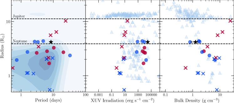
Figure 1: A panel of exoplanet demographics information from the NASA Exoplanet Archive as of August 2022. Non-specified, field-age planets are represented by the light blue contours and light blue triangles. Specified planets have been searched for atmospheric escape. Filled circles indicate at least one published detection of hydrogen and/or helium escape. The x’s indicate hydrogen/helium escape non-detections. Among the detections/non-detections, field-age planets are dark blue, whereas young planets are red. The black star represents AU Mic b, with its range in bulk density showing its spread in mass measurements. The leftmost panel shows the distribution of exoplanets in radius and period. The center panel is exoplanet radius versus its X-ray to ultraviolet irradiation (Foster et al., 2022). The rightmost panel shows exoplanet radius versus bulk density limited to planets with $\sigma_{\rho}<0.1\rho$.

Gl 436b, GJ 3470b, and HAT-P-11b all belong to field age systems with ages $>1$ Gyr. It has been suggested, based on recent constraints on the orbital structures of Gl 436b and GJ 3470b, that these older planets experiencing mass loss may have undergone late migration after some gravitational disturbance to its original far-away orbit (Bourrier et al., 2022; Stefànsson et al., 2022). HD 63433c is the only young planet with a detection of escaping neutral hydrogen. Two other young Neptunes, HD 63433b and K2-25b, have Ly$\alpha$ transit observations, neither of which exhibit escaping neutral hydrogen (Zhang et al., 2022a; Rockcliffe et al., 2021). This provokes interesting questions about the detectability or presence of atmospheric escape in young Neptune-sized planets. Rockcliffe et al. (2021) describe multiple scenarios to reconcile the detected escaping atmospheres with the non-detections. For example, is the amount of ionizing radiation or strength of the stellar wind coming from a young star too great to allow a large planetary neutral hydrogen outflow to develop? These questions warrant more Ly$\alpha$ transit observations of young exoplanet atmospheres.

Table 1: AU Mic system properties.

Properties (Symbol)	Value	Units	Reference
Earth-system distance (d)	$9.722100\pm 0.0004625$	pc	Gaia Collaboration et al. (2018)
Age ($\tau$)	$22\pm 3$	Myr	Mamajek & Bell (2014)
Right ascension ($\alpha$)	20:45:09.87	hh:mm:ss	…
Declination ($\delta$)	$-$31:20:32.82	dd:mm:ss	…
Spectral type	M1Ve		Turnbull (2015)
Bolometric luminosity (L${}_{\text{bol}}$)	$0.09$	L⊙	Plavchan et al. (2009)
Stellar mass (M⋆)	$0.50\pm 0.03$	M⊙	Plavchan et al. (2020)
Stellar radius (R⋆)	$0.75\pm 0.03$	R⊙	White et al. (2019)
Stellar rotation period (P⋆)	$4.863\pm 0.010$	days	Torres et al. (1972)
Radial velocity (v⋆)	$8.7\pm 0.2$	km s-1	Lannier et al. (2017)
Epoch (t0)	$2458330.39080^{+0.00058}_{-0.00057}$	BJD	Gilbert et al. (2022)
Transit duration	$3.56^{+0.60}_{-0.46}$	hours	Gilbert et al. (2022)
Planetary mass measurements (M${}_{\text{p}}$)	$11.7^{+5.0}_{-5.0}$	M⊕	Zicher et al. (2022)${}^{\text{a}}$
…	$17.0^{+5}_{-5}$	M⊕	Martioli et al. (2021)${}^{\text{b}}$
…	$17.1^{+4.7}_{-4.5}$	M⊕	Klein et al. (2021)${}^{\text{a}}$
…	$20.12^{+1.57}_{-1.72}$	M⊕	Cale et al. (2021)${}^{\text{a}}$
Planetary radius (R${}_{\text{p}}$)	$4.19^{+0.24}_{-0.22}$	R⊕	Gilbert et al. (2022)
Orbital period (P${}_{\text{p}}$)	$8.4630004^{+0.0000058}_{-0.0000060}$	days	Gilbert et al. (2022)
Semi-major axis (a)	$0.0644^{+0.0056}_{-0.0054}$	AU	Gilbert et al. (2022)

AU Mic is an M1Ve star in the $\beta$ Pic moving group (Zuckerman & Song, 2004) with a reliably constrained age of $23\pm 3$ Myr (Mamajek & Bell, 2014). At $9.79\pm 0.04$ pc, it is one of the closest pre-main sequence stars to Earth. Two exoplanets transiting AU Mic have been discovered using data from TESS (Gilbert et al., 2022; Martioli et al., 2021; Plavchan et al., 2020). AU Mic b orbits closer to its host, with a period of $8.46$ days. An overview of AU Mic’s system parameters, excluding AU Mic c, is given in Table 1. Gilbert et al. (2022) measured AU Mic b’s radius as $4.19$ R_⊕, placing it on the edge of the hot Neptune desert as shown in the left-most panel of Figure 1. We expect planets of this size (indicating a large gaseous envelope) and orbital period (highly irradiated) to be experiencing significant photoevaporation. This and the star’s youth and proximity to Earth prompt the detailed study of AU Mic b’s potentially escaping atmosphere. We obtained Ly$\alpha$ transits of AU Mic b with HST/STIS (HST-GO-15836; PI: Newton). These observations are presented in Section 2. We analyze the presence and impact of an observed stellar flare in Section 3. After accounting for the flare, we search for the presence of planetary absorption in Ly$\alpha$ and other emission line light curves in Section 4. We confirmed that AU Mic c does not transit during our observations. We also shifted the white-light mid-transit time for each visit (the zero hour mark in Figures 6, 7, 8, and 9) in line with recent transit-timing variation analyses for the AU Mic system (Wittrock et al., 2022). We construct the high energy environment of AU Mic b, and estimate its mass loss rate and the impact of photoionization in Section 5. We summarize and discuss our results in Section 6.

2 Far-UltraViolet Observations

2.1 New observations corresponding to two transits of AU Mic b

We obtained FUV observations of AU Mic using a $0.2$″ x $0.2$″ aperture on HST’s STIS instrument. HST observed the AU Mic system on 2 July 2020 (Visit 1) and 19 October 2021 (Visit 2), corresponding to two transits of AU Mic b. Six science exposures were taken per transit, each exposure covering the observable window of an HST orbit ($2000-3000$ s). STIS was in its FUV multi-anode microchannel array configuration (FUV-MAMA). We used the E140M echelle grating, which has a resolving power of $\sim 45800$ and wavelength coverage from $1144-1729$ Å. All science observations were made in TIME-TAG mode, where each photon detected by the instrument has a time-stamp. The time-stamps allowed us to split each science exposure into smaller sub-exposures prior to data extraction and reduction. This was done using the inttag function from the stistools Python package (v1.3.0). For our flare analysis in Section 3, we used $30$ s sub-exposures. Shorter sub-exposures were too low signal. We used 10 sub-exposures ($\sim 241$ or $275$ s each) per orbit for our light curve analysis in Section 4. We extracted and reduced these data with stistools.x1d.x1d, which utilizes the calstis pipeline (v3.4). We allowed the pipeline to find the best extraction location per echelle order in the calibrated, flat-fielded exposures. The extraction locations per echelle order varied by less than a pixel between each orbit. The same extraction and reduction procedure was used on the sub-exposures. Each reduced spectrum contains 44 echelle orders.

The pipeline uncertainties correlate with $\sqrt{\text{N}}$, where N is the total photon count per wavelength bin. This uncertainty estimate is inaccurate for small counts, which is the case for the lower signal-to-noise sub-exposures. As in Rockcliffe et al. (2021), we recalculated the errors for each sub-exposure spectrum using Equation 1, an estimation of the confidence limit of a Poisson distribution, and the total counts reported in the GROSS spectrum. These uncertainties were converted from counts into flux units using a multiplicative factor inferred by comparing the GROSS and flux-calibrated spectra. The calstis errors were used for the full-orbit spectra, which are high signal-to-noise.

$$\sigma\approx 1-\sqrt{\text{N}+0.75}$$ (1)

2.2 Investigating breathing

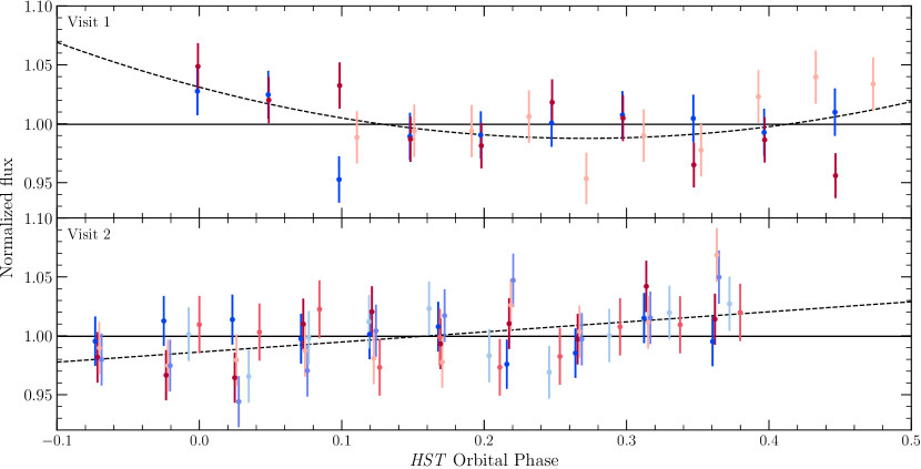
Figure 2: Visits 1 and 2 Ly$\alpha$ light curves folded on the HST orbital period ($95.42$ min). Each color corresponds to sub-exposures from a single HST orbit. Only sub-exposures from consecutive orbits are plotted (and considered in fitting the trend). The best-fit polynomial is shown by the dashed line.

Before analysis, we sought to remove HST “breathing” - thermal fluctuations that cause variability in the telescope optics, impacting the throughput on the timescale of an HST orbit ($95.42$ min). For each transit, we created a light curve of consecutive orbits for the integrated Ly$\alpha$ line flux in each sub-exposure ($10$ per orbit). Ly$\alpha$ was integrated over $1214.0-1217.0$ Å (excluding the remnant airglow region between $1215.4$ and $1215.7$ Å). Ly$\alpha$ is the highest signal-to-noise emission line in our data and thus the most preferred region to search for systematics. However, we note that our detrending process may overcorrect potential planetary and stellar variability on the – relatively short – timescale of an HST orbit.

Figure 2 shows the Ly$\alpha$ light curves for Visits 1 and 2 folded on HST’s period and the corresponding best-fit polynomials. The flux values are normalized by the mean flux per HST orbit. The best-fit per light curve was determined by selecting the polynomial order that gave the smallest Bayesian Information Criteria (BIC). Both transits deviate from a flat line, which corresponds to variability over the course of an HST orbit and confirms the presence of “breathing”. To detrend, we divided the best-fit polynomial out of each folded light curve (non-consecutive orbits included). The same process was used to detrend each FUV emission line light curve because HST breathing has been characterized as an achromatic effect. Most emission line light curves were consistent with a flat line when folded.

2.3 Archival FUV observations

We reference archival HST/STIS observations of AU Mic published by Pagano et al. (2000). Four science exposures were taken on 06 September 1998, which does not correspond to an AU Mic b transit (HST-GO-7556; PI: Linsky). The observing set-up was the same as our observations: $0.2$″ x $0.2$″ aperture, FUV-MAMA configuration, E140M grating, TIME-TAG mode. The same extraction, reduction, and breathing-check processes were used on these data.

2.4 Looking for planetary absorption with Ly$\alpha$ and other emission line spectra

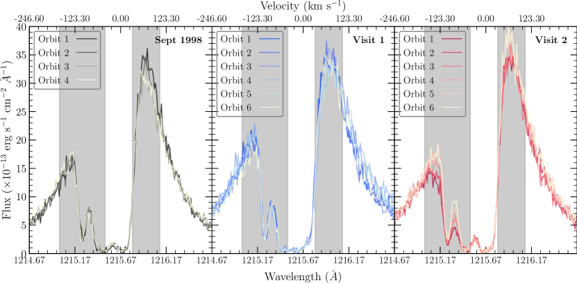
Figure 3: The Ly$\alpha$ spectra of AU Mic observed by HST/STIS in September 1998 (left, archival), July 2020 (center, Visit 1), and October 2021 (right, Visit 2). The gray shaded areas indicate our blue- and red-wing integration regions.

Figure 3 depicts the observed Ly$\alpha$ spectra for each new visit alongside the archival data. The ISM absorbs the line core ($\sim 1215.67$ Å), leaving the wings for analysis. Although Ly$\alpha$ observations of high radial velocity stars are becoming more common (Youngblood et al., 2022; Schneider et al., 2019), young stars in particular are low in velocity and as such do not experience significant Doppler shifting of spectral lines. AU Mic’s low velocity ensures that the Ly$\alpha$ line core is unobservable at Earth due to absorption by the ISM. Both the archival and Visit 2 data have residual geocoronal emission within the wavelengths fully absorbed by the ISM. Due to the high spectral resolution of STIS echelle data, this is not important for our analysis.

Although the Visit 1 Ly$\alpha$ spectra remain fairly consistent throughout the transit, the flare addressed in Section 3 is encapsulated in its first orbit. Due to the flare’s short duration, it is washed out by the full-orbit exposure time and a flux increase is not visible. The flare still has the ability to impact our search for planetary absorption, however, and this first orbit cannot be considered devoid of any contamination despite its stable appearance. When discussing the full-orbit spectra, we ignore this orbit.

Over all three visits to AU Mic, the extended blue-wing ($\lambda<1215$ Å) remains stable. This may indicate that the blue-wing is relatively impervious to stellar activity. The same cannot be said for the extended red-wing ($\lambda>1216.1$ Å), which shows variations of up to $10\%$ percent in the archival, Visit 1, and Visit 2 data (see Figure 8). The inner red-wing – where we are looking for planetary absorption ($1215.8<\lambda<1216.1$ Å; $32.1<v<106$ km s^-1) – shows similar fluctuations across the three visits. It may be that the entirety of the Ly$\alpha$ red-wing is more sensitive to stellar activity than its blue counterpart. For that reason, we hesitate to associate a decrease in the Ly$\alpha$ red-wing flux up to about $10\%$ with planetary absorption.

Table 2: Best-fit parameters with $1-\sigma$ uncertainties for the in-transit (Visit 2, first orbit) and out-of-transit (Visit 2, sixth orbit) Ly$\alpha$ spectra: characterizing the intrinsic Ly$\alpha$ line, the ISM absorption, and the planetary absorption.

Parameter (Units)	In-Transit Value	Out-of-Transit Value
v${}_{\text{n}}$ (km s-1)	…	$-7.29^{+0.92}_{-0.89}$
log10A${}_{\text{n}}$ (erg s-1 cm-2 Å-1)	…	$-10.87^{+0.03}_{-0.03}$
FW${}_{\text{n}}$ (km s-1)	…	$140.54^{+2.82}_{-2.74}$
v${}_{\text{b}}$ (km s-1)	…	$-7.37^{+1.18}_{-1.18}$
log10A${}_{\text{b}}$ (erg s-1 cm-2 Å-1)	…	$-11.64^{+0.02}_{-0.02}$
FW${}_{\text{b}}$ (km s-1 )	…	$386.12^{+6.03}_{-5.87}$
ISM log10N${}_{\text{H I}}$	…	$18.38^{+0.01}_{-0.01}$
b (km s-1)	…	$12.34^{+0.27}_{-0.29}$
v${}_{\text{H I}}$ (km s-1)	…	$-22.98^{+0.23}_{-0.23}$
pl log10N${}_{\text{H I}}$	$13.96^{+0.03}_{-0.03}$	…
b${}_{\text{pl}}$ (km s-1)	$61.05^{+2.24}_{-2.24}$	…
v${}_{\text{pl}}$ (km s-1)	$-61.26^{+2.45}_{-2.74}$	…

We expect the majority of escaping planetary material to be moving at $10$s of km s^-1. Hydrodynamic models show that radiation and stellar wind pressure can accelerate escaping neutral hydrogen up to these velocities directed radially outward from the host star (McCann et al., 2019; Bourrier et al., 2018). This draws our attention to the inner blue-wing ($1215<\lambda<1215.5$ Å; $-165.2<v<-41.9$ km s^-1) which could be experiencing flux variations due to absorption by planetary neutral hydrogen flowing away from the host star. The archival spectra do not show any significant changes within this region. The Visit 1 spectra display a small amount of variability at the shorter wavelength edge of our blue-wing region. The Visit 2 spectra, however, show a gradual $30\%$ increase in the blue-wing flux over the course of the planet’s transit.

Assuming the flux behavior is due to absorption by escaping planetary neutral hydrogen, we fit the observed Ly$\alpha$ profile with an intrinsic stellar component, an ISM absorption component, and a planetary absorption component. We used the Python package lyapy (Youngblood & Newton, 2022), which encompasses a model that combines the aforementioned emission and absorption components and a fitting algorithm that uses emcee as the MCMC sampler (Foreman-Mackey et al., 2013). A thorough description of the lyapy model and how it can be used to reconstruct cool star Ly$\alpha$ emission profiles can be found in Youngblood et al. (2016) and Section 4.1 of Raetz et al. (2020).

First, we reconstructed AU Mic’s Ly$\alpha$ emission line using the last orbit from Visit 2 (see right panel of Figure 4), which we assume is out-of-transit for the planetary neutral hydrogen. The timing of absorption in comparison to the planet’s white-light transit is discussed more thoroughly in Sections 4 and 6. We varied every stellar and ISM profile parameter with uniform priors except for the ISM deuterium-to-hydrogen ratio, which we fixed to $1.5\times 10^{-5}$ (Linsky et al., 2006). The best-fit parameters that recreated our observed Ly$\alpha$ profile can be found in Table 2. Our results do not agree within uncertainties with the reconstructed AU Mic Ly$\alpha$ profile from Youngblood et al. (2016) (see their Table 1). However, our best-fit values agree within a few $\sigma$ at most and the stability of M dwarf Ly$\alpha$ emission at young ages has not been fully explored.

We modified the absorption model within lyapy to include a Voigt profile characterizing the excess absorption due to the proposed planetary outflow. This profile is only able to characterize the high velocity outflow that is visible in our observations. All information regarding the low velocity planetary material is lost due to ISM absorption. The profile is parameterized by column density, Doppler broadening, and a velocity centroid associated with the intervening planetary neutral hydrogen. These three parameters were varied during our fit to the in-transit spectrum, whereas our best-fit Ly$\alpha$ emission and ISM absorption values from the out-of-transit profile were fixed. We estimate the high velocity planetary neutral hydrogen has a column density of log₁₀N${}_{\text{H I}}=13.96^{+0.03}_{-0.03}$ and is moving $-61.26^{+2.45}_{-2.74}$ in the stellar rest frame. Our column density should be treated as a lower limit on the total neutral hydrogen column density of the outflow. The left panel of Figure 4 shows the best-fit planetary absorption scaled to the figure’s y-axis along with the best-fit to the observed spectrum. We investigate this in-transit absorption further by integrating over the region and analyzing the light curve in Section 4.

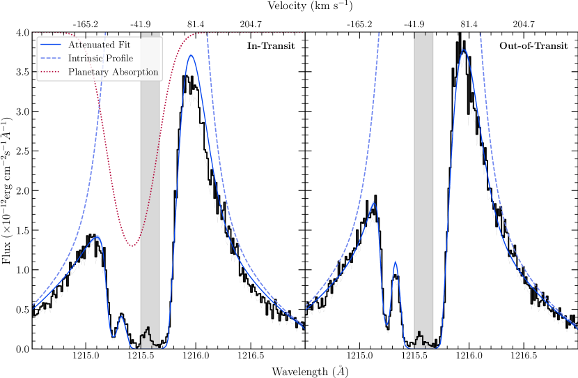
Figure 4: The AU Mic Ly$\alpha$ spectra “in-transit” on the left (Visit 2 first orbit) and “out-of-transit” on the right (Visit 2 sixth orbit). The observed data is shown by the black line. The blue dashed line is the reconstructed stellar Ly$\alpha$ line. The Voigt profile fit for the planetary absorption scaled to the y-axis of the figure is represented by the red dotted line. The blue line is the best fit damped Ly$\alpha$ profile, with its $1-\sigma$ uncertainty shown by shaded blue regions around the line. The gray shaded regions indicate areas of the data that were masked before being run through our fitting algorithm.

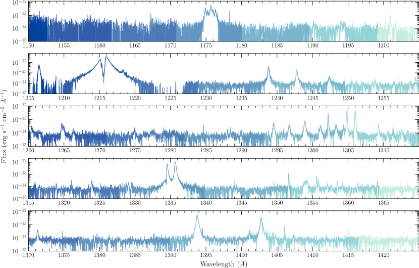
Figure 10: AU Mic’s quiescent spectrum – the last orbit from Visit 1. Continued in Figure 11.

Figure 5 shows the archival, Visit 1, and Visit 2 spectra for the N V, O I, Si IV, He II, and C I species. Although there are more emission lines present in the data (see Table 3 and Figures 10 and 11), we focus on these five species for tracing stellar activity and our search for planetary atmospheric escape. FUV spectroscopic studies of M dwarfs have shown that N V and Si IV can trace stellar activity, which can help identify when flux changes are not planetary in nature (Loyd et al., 2018b; Loyd & France, 2014). Alternatively, O I, He II, and C I are relatively insensitive to flares. O I and C I are of recent interest as potential tracers of the evolution of the C/O ratio in exoplanet atmospheres (Owen, 2022). O I, C I and C II have been used to trace atmospheric escape previously in several hot Jupiters, as well as the hot super Earth $\pi$ Men c (García Muñoz et al., 2021).

As expected, the Visit 1 flare causes substantial increases in the emission line fluxes for N V and Si IV, whereas O I and C I do not. He II also experiences an enhancement due to the flare. In Visit 2, N V and He II have a similar flux increase during the fifth orbit, which also corresponds to the increase observed in the Ly$\alpha$ blue-wing in Figure 3 but does not last through the sixth orbit. When compared to the archival spectra, this behavior is not representative of the typical noise in N V and He II emission. Light curves for these two species are presented in Section 4 and compared to the Ly$\alpha$ line behavior. O I shows consistent spectral variation across the archival, Visit 1, and Visit 2 spectra, making it difficult to discern the presence of planetary absorption. Similarly, C I is too low signal-to-noise to draw any conclusion about carbon in transmission. Their light curves are also shared in Section 4.

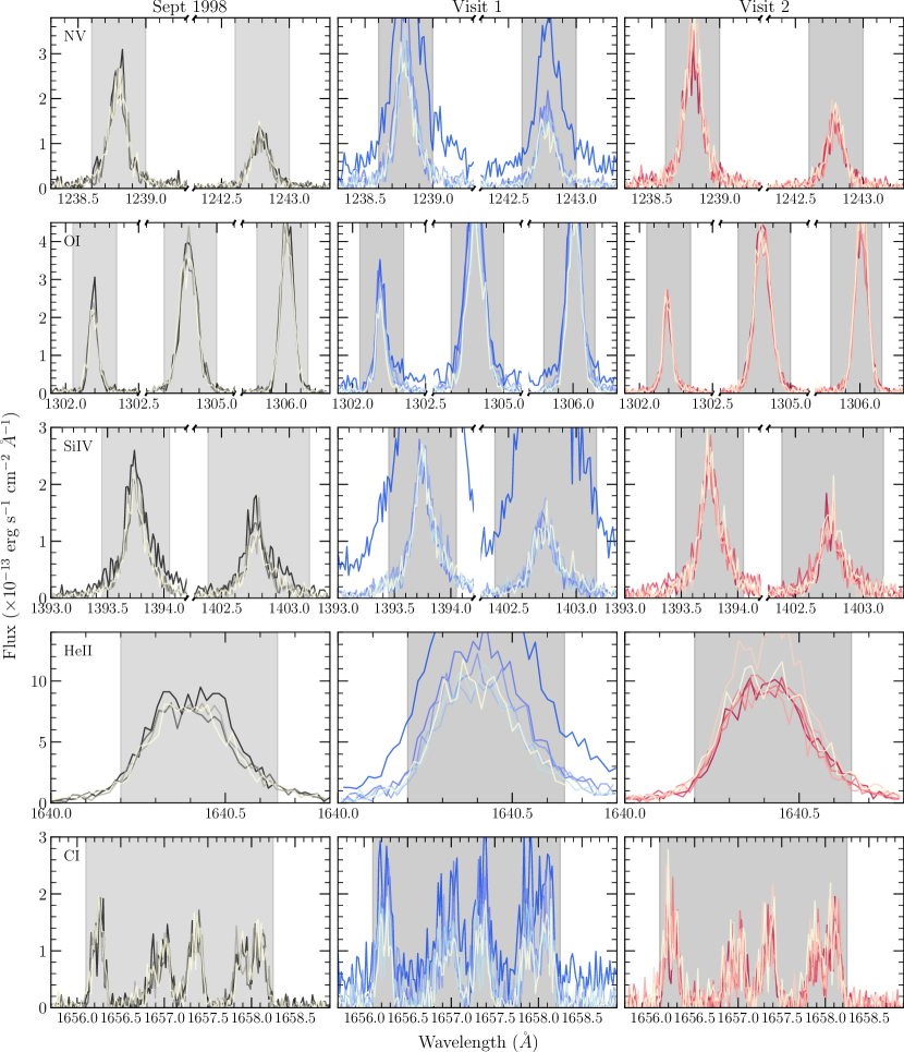
Figure 5: The emission line spectra of AU Mic observed by HST/STIS in September 1998 (left, archival), July 2020 (center, Visit 1), and October 2021 (right, Visit 2). The gray shaded areas indicate our integration regions. The orbits correspond to the same colors indicated in Figure 3.

Table 3: AU Mic FUV emission lines confidently identifiable in this work’s HST/STIS spectra, cross-referenced with NIST (Kramida et al., 2021), the CHIANTI Atomic Database (Del Zanna et al., 2021; Dere et al., 1997), and Feinstein et al. (2022). The table includes line location(s), integration region, and formation temperature.

Species	$\lambda$ (Å)	$\Delta\lambda$ (Å)	$\log_{10}(T/\text{K})$
C III	$1175.7$	$1174.5-1177.0$	$4.8$
Si III	$1206.51$	$1206.3-1206.7$	$4.7$
H I (Ly$\alpha$)	$1215.67$	$1214.0-1217.0$	$4.5$
N V	$1238.82$, $1242.80$	$1238.6-1239.0$, $1242.6-1243.0$	$5.2$
O I	$1302.2$, $1304.84$, $1306.01$	$1302.05-1302.35$, $1304.7-1305.0$, $1305.8-1306.15$	$3.8$
C II	$1334.53$, $1335.71$	$1334.45-1334.75$, $1335.45-1335.95$	$4.5$
Fe XXI	$1354.07$	$1353.8-1354.4$	$7.1$
Si IV	$1393.76$, $1402.77$	$1393.45-1394.05$, $1402.4-1403.15$	$4.9$
C IV	$1548.20$, $1550.774$	$1547.9-1548.5$, $1550.6-1551.0$	$4.8$
He II	$1640.40$	$1640.2-1640.65$	$4.9$
C I	$1656.27$, $1656.93$, $1657.01$, $1657.38$, $1657.91$, $1658.12$	$1656.0-1658.25$	$3.8$

3 Flare Analysis

3.1 Emission line flare light curves

Before looking for a planetary signature, we needed to characterize and remove any host star variability from our observations. A substantial increase in AU Mic’s flux in several emission lines and its FUV continuum occurred during the first orbit of Visit 1, initially identified by eye. Figure 6 shows the diversity in flaring behavior of the highest signal-to-noise emission lines (listed in Table 3). We used $30$ s sub-exposures for comprehensive sampling of the flare. We did not model these light curves as we did with Ly$\alpha$ and the continuum presented in Section 3.2.

As shown in Figure 6, C III, Si IV and C IV exhibit the strongest emission during the peak of the flare, followed by Si III and C II. Most emission lines return to quiescent fluxes relatively quickly ($\sim 2$ min). A notable exception is He II, which remains elevated over the entirety of the exposure and returns to quiescence by the second exposure (not pictured). The Visit 1 flare caused greater flux increases in every overlapping emission line examined between this work and Feinstein et al. (2022). However, caution should be taken when comparing fluxes observed with STIS and COS, as STIS has focus issues that impact the flux calibration of narrow slit observations (Riley et al., 2018; Proffitt et al., 2017). The one flare we observe in our $\sim 7$ hours of non-consecutive HST orbits is at odds with the $2.5$ hour^-1 AU Mic FUV flare rate presented in Feinstein et al. (2022) and potentially agrees with the $2$ day^-1 estimate from Gilbert et al. (2022) based on visible light data. Although we did not conduct further analysis, characterizing this flare and comparing it to other AU Mic flares observed with STIS and COS would further knowledge of flare diversity from an individual star and help identify systematic differences between the STIS and COS instruments.

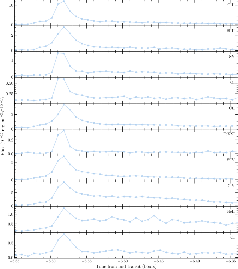
Figure 6: Light curves for the first orbit of Visit 1 split into $30$ s sub-exposures for various emission lines from Table 3.

3.2 Ly$\alpha$ and continuum flare modeling

Flares and other forms of stellar activity can mask or masquerade as planetary signals in transit photometry and transmission spectroscopy. Loyd & France (2014) surveyed 38 cool stars with HST/COS and STIS spectra, characterizing their variability in the ultraviolet and the potential for masking planetary signals. They concluded that most F-M stars will allow for confident detections of planets larger than Jupiter, with M dwarfs potentially lowering that limit to Neptune-to-Saturn-sized planets.

We modeled the Visit 1 flare in order to characterize its potential to mask the transit of AU Mic b. For this analysis, we focused on the Ly$\alpha$ emission line because it is the highest signal emission line in the data and because of its relevance to our search for atmospheric escape in transmission. We also modeled the FUV continuum behavior during the flare for comparison (continuum defined in A.1).

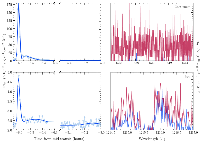
Figure 7: Continuum (top, left) and Ly$\alpha$ (bottom, left) light curves for the first two orbits of Visit 1. The light blue points are the $30$ s sub-exposures, and the blue line is the fitted flare model. Continuum and Ly$\alpha$ in- (red) and out-of-flare (blue) spectra are shown in the top-right and bottom-right panels, respectively.

We adapted the open source Python code cos_flares from Feinstein et al. (2022) written for analyzing flares in HST/COS data to be compatible with our STIS data. We fit the Visit 1 flare light curve using a skewed Gaussian, represented by Equation 2 where $\omega$ parameterizes the amplitude, $t$ is time, $\xi$ is the average time in the flare light curve, and $\eta$ is a dimensionless version of time related to the aforementioned parameters and the skewness of the light curve. The skewed Gaussian model was chosen because it provided the best fit to the Ly$\alpha$ light curve compared to the white-light flare model and the skewed Gaussian convolved with the white-light flare model. Figure 7 shows the resulting fit to the Ly$\alpha$ flare. We allowed for multiple peaks in the flare to be modeled and fit, which is shown by the small increase in flux after the flare.

$$F(t)\sim\frac{1}{\omega\sqrt{2\pi}}\left(e^{-(t-\xi)^{2}/(2\omega)^{2}}\right)\left[1+\text{erf}\left(\frac{\eta}{\sqrt{2}}\right)\right]$$ (2)

3.3 Flare energy and duration

We calculated the flare energy, equivalent duration, and maximum time the flare could mask a $10\%$ planetary transit.

Absolute flare energy, $E$, is the total energy released by the flare at the star within the spectral feature. It is given by Equation 3:

$$E=4\pi d^{2}\int\left(F_{f}(t)-F_{q}(t)\right)dt$$ (3)

where $d$ is the distance to AU Mic, and $F_{fl}$ and $F_{q}$ are the flaring and quiescent fluxes (Davenport et al., 2014; Hawley et al., 2014). The difference in flaring and quiescent flux is integrated over the time it takes for the flux to return to quiescence. We classified the first two orbits of Visit 1 as flaring, and the remaining out-of-transit orbit at the end of the visit as quiescent.

We calculated a total flare energy of $7.11\times 10^{32}$ erg for Ly$\alpha$, and $2.57\times 10^{34}$ erg for the continuum. Our continuum flare energy is $100$ times larger than the median flare energy characterized in Feinstein et al. (2022) for AU Mic. It is also $1000-10000$ times larger than the median FUV flare energy found by surveying M stars (Loyd et al., 2018a, b).

The equivalent duration, $t_{eq}$, is given by Equation 4. Similar to an equivalent width, it characterizes the amount of time for which the star would have to emit 100% of its quiescent flux in order to match the total energy of the flare. The flare’s equivalent duration was estimated as $278$ s ($0.0772$ hours) for Ly$\alpha$, and $43515$ s ($12.1$ hours) for the continuum.

$$t_{eq}=\int\left(\frac{F_{f}(t)-F_{q}(t)}{F_{q}(t)}\right)dt$$ (4)

The maximum masking time bears the most importance to our search for AU Mic b in transmission. We calculated the amount of time the flare was above $110\%$ of the quiescent Ly$\alpha$ flux, effectively washing out a $10\%$ planetary transit depth. We chose $10\%$ as a conservative estimate for the potential size of the exosphere. We found that this flare contaminated the Ly$\alpha$ light curve for about $5731$ s, or $1.5$ HST orbits. This occurred 7 hours before AU Mic b’s white-light mid-transit, so we do not expect the increase in flux from the flare to deter us from observing a planetary signal in Visit 1.

4 AU Mic’s Light Curves

We examined the temporal behavior of AU Mic’s flux in different regions of its FUV spectrum (i.e., the Ly$\alpha$ emission line and the several metal lines listed in Table 3). In Section 3 we concluded that the flare only impacts the first orbit of Visit 1, so we removed the contaminated orbit and examined the Visit 1 and 2 light curves separately for signs of planetary absorption.

4.1 Ly$\alpha$ light curve

The presence or absence of absorption in the Ly$\alpha$ line over the course of AU Mic b’s transit can indicate whether or not neutral hydrogen is escaping from the planet’s upper atmosphere. After the detrending process described in Section 2, we created two Ly$\alpha$ light curves per transit by summing the flux in the blue-wing ($1215.0-1215.5$ Å) and the red-wing ($1215.8-1216.1$ Å). The errors were summed in quadrature. Visit 1 exposures were normalized by the sixth orbit, which occurs $17$ hours after mid-transit and $>20$ hours after the flare. Visit 2 was normalized by the average of the fifth and sixth orbits. We also included archival HST/STIS observations of AU Mic from September 1998 which do not coincide with an AU Mic b or c transit, normalized by the last orbit from this visit. These light curves are shown in Figure 8.

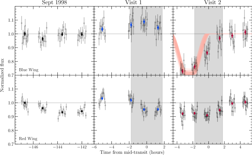
Figure 8: The archival (left, black), Visit 1 (center, blue), and Visit 2 (right, red) light curves for the blue- (top) and red-wing (bottom) of the Ly$\alpha$ line. The first orbit from Visit 1 is not included because of the flare. Visit 1’s sixth, and final, orbit is not included but is represented by the horizontal line at a flux of 1. The gray points represent the sub-exposures. Samples from the posterior distribution of light curve fits to the Visit 2 blue-wing are shown by the pink lines. The white-light transit duration is shown by the gray shaded region.

The Ly$\alpha$ blue-wing shows a $\sim 5\%$ increase in emission during Visit 1 (center-top panel of Figure 8). For this reason, we do not attempt to fit for a planetary transit in this light curve. We present possible explanations for this in Sections 4.2 and 6. As discussed in Section 2, the Ly$\alpha$ red-wing exhibits consistent flux changes of up to $10\%$ across all three HST visits. These fluctuations occur at different times in relation to the planetary ephemeris – from $100$s to within a few hours outside of transit – leading us to conclude that these are changes in the intrinsic stellar Ly$\alpha$ emission.

The Visit 2 Ly$\alpha$ blue-wing light curve exhibits extended absorption starting at least four hours prior to the white-light mid-transit. The blue-wing flux decrease lasts for about four hours and is completely recovered by the conclusion of white-light transit. If the decrease in flux is due to absorption in AU Mic b’s atmosphere, that implies that the neutral hydrogen is moving ahead of the planet and is expanding radially away from the host star. We pose physical explanations for the bulk of the escaping atmosphere to transit before the planet in Section 6. Although slight Ly$\alpha$ absorption prior to planet transit has been observed in other systems, like GJ 3470b, it has never been observed to this magnitude (Bourrier et al., 2018).

Table 4: Fixed Light Curve Parameters (Gilbert et al., 2022).

Parameter	Value	Units
$P_{\text{p}}$	$8.4630004$	days
$a$	$0.0644$	AU
$i$	$89.18$	degrees
$e$	$0.12$
$w$	$88.528$	degrees

We used batman to model a planetary transit for the Visit 2 blue-wing and emcee to explore parameter space using Markov Chain Monte Carlo (MCMC). batman models a transit for a fully opaque circle, not allowing for more diverse atmospheric geometries. We initialized the batman model with measured system parameters (see Table 4). Only the planetary radius at Ly$\alpha$ and the mid-transit time were free parameters. The mid-transit time had a uniform prior constrained to within 5 hours of the white-light mid-transit time. The planetary radius at Ly$\alpha$ was limited to positive values (no negative transit depths). The 60 sub-exposures associated with Visit 2 were fit using 80 MCMC walkers and 200000 steps. There was a burn-in of 50000 steps. We did the same for the Visit 2 red-wing, but the opaque disk model provides a poor fit to our data due to its long duration and small flux decrease.

The best-fit $R_{\text{p}}/R_{\star}$ value for the blue-wing light curve is $0.52\pm 0.01$ ($0.39\pm 0.008$ R_⊙). The Ly$\alpha$ blue-wing mid-transit time is $2.5\pm 0.24$ hours before the white-light mid-transit time. Figure 8 includes example light curves pulled from the MCMC posteriors as pink lines. A model that allows for non-circular geometries and/or transparency of the transiting object along with data corresponding to the beginning of the absorption signal would be required to better fit our blue-wing light curve.

We used the formalism presented in Owen et al. (2023) to estimate the geometry and kinematics of the escaping planetary material. Although they model a trailing tail of neutral hydrogen, the same physics applies to a leading tail – our observations of AU Mic b correspond to a flipped version of Figure 1 from Owen et al. (2023). We used their Equations 10 and 11 for transit depth and duration, respectively, to calculate a tail length of $9.69\times 10^{10}$ cm ($1.39$ R_⊙) and height of $2.22\times 10^{10}$ cm ($0.32$ R_⊙). From their Equation 2, we estimated the velocity of the bulk of escaping material – before acceleration by interactions with the environment – to be $20$ km s^-1. Unfortunately we are unable to probe this velocity observationally for the AU Mic system due to the ISM absorption at the Ly$\alpha$ core (see Section 2.4), but Ly$\alpha$ observations of high radial velocity systems allow transits to occur at these lower velocities, as do transits of uncontaminated emission lines (e.g., He $10830$ Å). As specified by Owen et al. (2023), we treat these calculations as rough estimates to be tested by future sophisticated models.

4.2 Metal line light curves

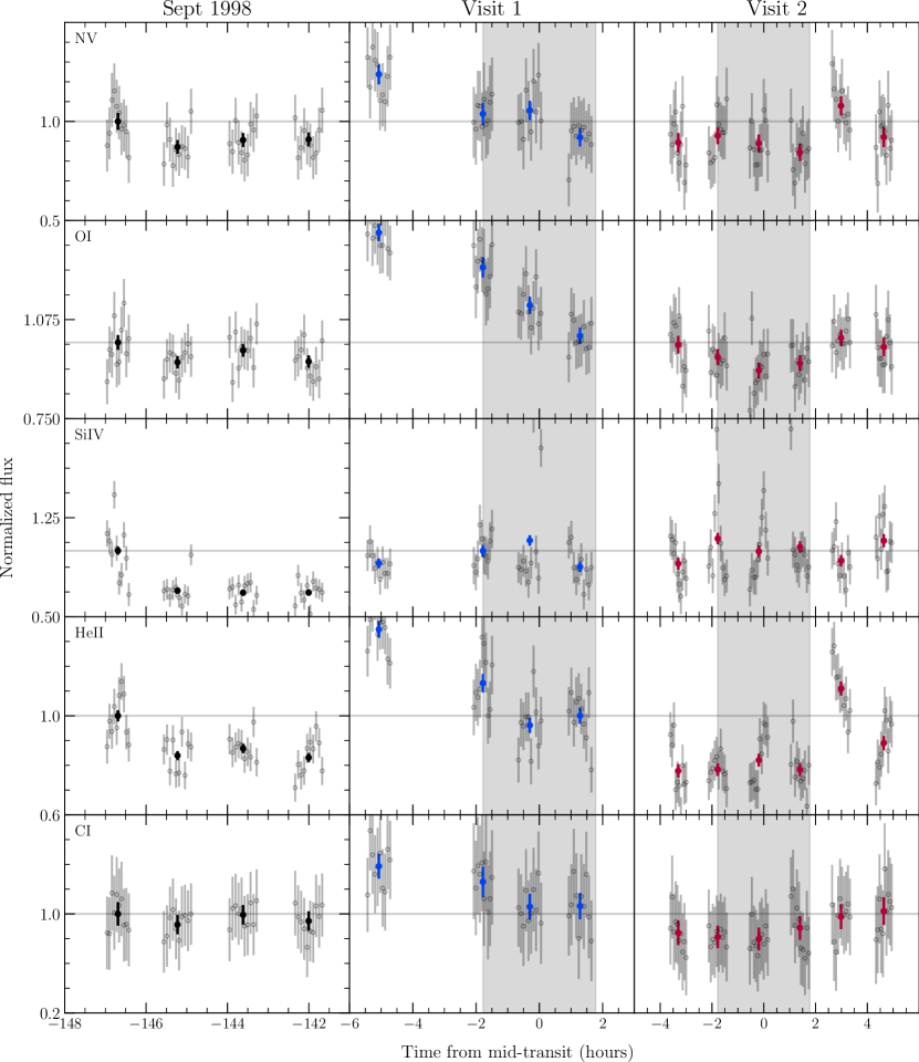
Figure 9: The archival (left, black), Visit 1 (center, blue), and Visit 2 (right, red) light curves for several FUV emission lines. The first orbit from Visit 1 is not included because of the flare. Visit 1’s sixth, and final, orbit is not included but is represented by the horizontal line at a flux of 1. The gray points represent the sub-exposures. The white-light transit duration is shown by the gray shaded region.

The search for atomic metals has been ongoing in some of the hottest giant planet atmospheres. Detections of atomic sodium, potassium, and calcium have come from optical and infrared observations (e.g., Zhang et al., 2022b; Hoeijmakers et al., 2020; Yan et al., 2019). Using HST/STIS, neutral and ionized metals (mostly sodium) have been detected in the ultraviolet for several Hot Jupiters (Sing et al., 2019; Alam et al., 2018; Sing et al., 2016; Nikolov et al., 2014). With HST/COS, metal absorption extending past the Roche lobe has been detected for WASP-12b, showing that these ionized metals can be carried far away from the planet by atmospheric escape (Haswell et al., 2012; Fossati et al., 2010). Hot Neptunes, despite being more vulnerable to an escaping atmospheric outflow that could carry heavier atoms, have remained undetected in metal lines with the exception of sodium detected in WASP-166b (Seidel et al., 2022, 2020) and a potential detection of C I in HAT-P-11b (Ben-Jaffel et al., 2022).

Our AU Mic observations have a high enough signal-to-noise to look for transits of AU Mic b’s escaping atmosphere in the host’s metal emission lines. Figure 9 shows the light curves during Visits 1 and 2 for N V, O I, Si IV, He II, and C I. All lines show decreasing flux around AU Mic b’s mid-transit in Visit 1 except the slight emission shown by Si IV. It may be that the flare has a longer lasting impact on these metal lines as opposed to the one-orbit impact estimated for Ly$\alpha$ and so they are still evolving towards quiescence during the planetary transit.

The Visit 2 N V, O I, He II and C I light curves have a similar shape to the Visit 2 Ly$\alpha$ light curves in Figure 8, but with much lower signal-to-noise. N V and He II, two lines where we do not expect to see planetary material, exhibit the most pronounced transit-like behavior. The transit-like depth is reduced when the flux normalization is changed from the average between the fifth and sixth orbits to just the sixth orbit. The transit-like shape is also exhibited by the archival N V and He II light curves, which are well out of transit. As in Duvvuri et al. (2023), we speculate that the metal line variability is due to some uncharacterized stochastic stellar activity potentially linked to magnetic heating processes within AU Mic’s atmosphere. We encourage the use of this data in combination with future UV programs targeting M dwarfs to further investigate this non-flaring behavior.

The O I and C I light curves are of utmost interest when searching for planetary metal transits (Owen, 2022). Although the O I and C I light curves in Figure 9 depict transit-like behavior, we hesitate to characterize this as planetary absorption 1) because of the low signal from these lines and 2) because the behavior coincides with potential stellar activity signatures in the other emission lines presented. HST/COS will be more successful characterizing planetary metal line absorption than STIS. A metal outflow search is currently underway for AU Mic b using COS, which can be compared to these data to more definitively distinguish between planetary and stellar signatures (Feinstein, in prep).

5 AU Mic b’s High Energy Environment

We investigated the planet’s high energy irradiation to place constraints on how much mass it is potentially losing and how much of it is staying neutral. We define high energy irradiation as the quiescent radiation received between $5-1170$ Å, which covers the X-ray through the EUV. ROSAT observed AU Mic’s quiescent X-ray luminosity to be $2.51\times 10^{29}$ erg s^-1, corresponding to a flux of $21500$ erg s^-1 cm^-2 at AU Mic b (Table 3; Chadney et al., 2015).

Much of the star’s EUV spectrum is inaccessible due to obscuration by the intervening interstellar medium. Duvvuri et al. (2021) modeled AU Mic’s EUV spectrum using the differential emission measure technique. This method provides an estimate for the radiation from plasma at a specific temperature. They calculated an EUV flux of $8420$ erg s^-1 cm^-2 at AU Mic b. The combined XUV irradiation of the planet is about $29900$ erg s^-1 cm^-2.

Chadney et al. (2015) include X-ray and EUV luminosity measurements for a flaring AU Mic. Using the observed flare values from their Table 3, the combined flaring XUV irradiation of AU Mic b is $71500$ erg s^-1 cm^-2.

5.1 Planetary mass-loss rate

The amount of mass escaping the planet is often estimated by assuming the amount of high energy radiation received directly translates to heating the atmosphere, leading to a bulk flow of gas that overcomes the planet’s gravitational potential. This is referred to as the energy-limited regime. There are two other photoevaporation regimes that may apply: recombination-limited and photon-limited (Owen & Alvarez, 2016). The flow timescale to recombination timescale ratio determines which regime applies to a planet. This ratio is largely governed by the planet’s density and incident high energy flux. Figure $1$ in Owen & Alvarez (2016) shows how the three photoevaporation regimes depend on a planet’s mass and radius. Given AU Mic b’s XUV irradiation of $29900$ erg s^-1 cm^-2, it will likely follow the top left or bottom right panels depending on the atmosphere’s heating efficiency.

A typical source of uncertainty is the planet’s mass. This is difficult to measure with extreme precision and is yet more difficult for planets with active hosts, like AU Mic, due to contamination from stellar variability. There are a few mass measurements reported for AU Mic b: $11.7\pm 5.0$ M_⊕(Zicher et al., 2022), $17.1^{+4.7}_{-4.5}$ M_⊕ (Klein et al., 2021) and $20.12^{+1.57}_{-1.72}$ M_⊕ (Cale et al., 2021) from radial velocities, and $17\pm 5$ M_⊕ from transit-timing variations (Martioli et al., 2021).

AU Mic b has a radius of $2.60\times 10^{9}$ cm and a potential mass range of $6.99-12.0\times 10^{28}$ g. With a heating efficiency of $0.1$ (top left panel of Figure 1; Owen & Alvarez, 2016), AU Mic b will be within the energy-limited regime no matter its mass. However, if its atmosphere has a higher heating efficiency (bottom right panel of Figure 1; Owen & Alvarez, 2016), then the planet could enter the photon-limited regime. During periods of high stellar activity, if a lower mass AU Mic b’s XUV irradiation reaches $\gtrsim 10^{5}$ erg s^-1 cm^-2, then the planet could enter the recombination-limited regime. For this reason, we present AU Mic b’s energy-limited mass loss rate as a possible scenario but the true mass loss rate could be smaller or larger by a few orders of magnitude and will vary on short and long timescales.

The energy-limited regime is given by Equation 5, which is dependent on the incident high energy radiation ($F_{\text{XUV}}$), the planet’s radius ($R_{\text{p}}$) and mass ($M_{\text{p}}$), the atmosphere’s heating efficiency ($\eta$), and a correction factor ($K_{\text{eff}}$, Equation 6). $K_{\text{eff}}$ corrects for the difference in gravitational potential at the planet’s radius versus its Roche lobe where the atmosphere needs to escape.

$$\dot{M}=\eta\frac{\pi R^{3}_{\text{p}}F_{\text{XUV}}}{GM_{\text{p}}K_{\text{eff}}}$$ (5)

where:

$$K_{\text{eff}}=\frac{(a/R_{\text{p}}-1)^{2}(2a/R_{\text{p}}+1)}{2(a/R_{\text{p}})^{3}}$$ (6)

Assuming the properties listed in Table 1 and our quiescent XUV flux estimate, we estimate the energy-limited mass loss rate to be $(22.5-38.7)\eta\times 10^{10}$ g s^-1 for a mass range of $20.12-11.7$ M_⊕. We have not assigned a heating efficiency because it can vary widely across the exoplanet population (0.1 - 0.6; Shaikhislamov et al., 2014). The range presented is $100$ times larger than the AU Mic b mass loss rate estimated by Feinstein et al. (2022).

5.2 Photoionization rate

Radiation at wavelengths shorter than $912$ Å can ionize neutral hydrogen in exoplanet atmospheres. Large fluxes at these energies have the ability to ionize much of the gas that is escaping a planet. The observability of the atmosphere at Ly$\alpha$ depends on how much of the escaping material remains neutral for a long enough time to be accelerated to velocities that result in absorption in the line’s blue- and red-wings. To get an idea for how significantly photoionization impacts AU Mic b, we estimated the photoionization rate with the following equation that quantifies the amount of ionization events per unit time ($\Gamma_{\text{ion}}$; count s^-1):

$$\Gamma_{\text{ion}}=\int^{911.8\text{ \AA}}_{0\text{ \AA}}\frac{F_{\text{XUV}}(\lambda)\sigma_{\text{ion}}(\lambda)}{hc}\lambda d\lambda$$ (7)

where $F_{\text{XUV}}$ is AU Mic b’s wavelength-dependent XUV irradiation, and $\sigma_{\text{ion}}$ is the photoionization cross-section (cm²) defined by

$$\sigma_{\text{ion}}= 6.538\times 10^{-32}\left(\frac{29.62}{\sqrt{\lambda}}+1\right)^{-2.963}$$

$$\times(\lambda-28846.9)^{2}\lambda^{2.0185}.$$ (8)

We split Equation 7 into separate integrals over the X-ray ($5<\lambda\leq 100$ Å) and EUV ($100<\lambda\leq 912$ Å) spectral regions and summed them to get a photoionization rate of $4.01\times 10^{-4}$ s^-1. Inverting the photoionization rate characterizes the amount of time a typical neutral hydrogen atom stays neutral before interacting with an ionizing photon - the neutral hydrogen lifetime. A short neutral hydrogen lifetime indicates a smaller neutral atmosphere and likely a smaller Ly$\alpha$ transit depth and shorter transit duration.

At AU Mic b’s orbital distance, the neutral hydrogen lifetime is about $0.692$ hours (almost $42$ minutes) during quiescence, and decreases by about $50\%$ during a flare. This value is short compared to the benchmark planet Gl 436b, which has a neutral hydrogen lifetime of 14 hours and consequently a large trailing neutral hydrogen tail (Bourrier et al., 2016). It is not entirely impossible to observe planets with short neutral hydrogen lifetimes, however, as shown by the detection of neutral hydrogen around GJ 3470b (0.9 hours; Bourrier et al., 2018).

Owen et al. (2023) provide a theoretical framework that explains Ly$\alpha$ detections and non-detections of atmospheric escape with photoionization and the host star’s tidal influence. For example, the young Neptune K2-25b experiences enough XUV irradiation to have escaping material that is ionized and unobservable at Ly$\alpha$  resulting in a repeatable non-detection (Rockcliffe et al., 2021). A similar planet, HD 63433c, is less irradiated and is more likely to have escaping material detected at Ly$\alpha$ (Zhang et al., 2022a). There has not yet been Ly$\alpha$ observations of atmospheric escape on the same planet that vary to the degree we present in this work.

5.3 Recombination rate

If AU Mic b’s neutral hydrogen outflow is dense enough, the photoionization from the Visit 1 flare – and other instances of increased stellar emission – would be overcome by the recombination of ionized hydrogen back into its neutral state. In this case, we would not expect the flare to cause the non-detection of a Ly$\alpha$ transit in Visit 1. To test this, we estimated the recombination rate of AU Mic b’s outflow and compared it to the flare photoionization rate from Section 5.2.

The neutral hydrogen column density of $10^{13.96}$ cm^-2 estimated in Section 2.4 is a lower limit since it only characterizes the fastest escaping material. For this reason, we use the mass loss rate calculated in Section 5.1 and conservation of mass to estimate the total neutral hydrogen content of the outflow. Equation 9 exhibits this relationship, with $\rho$ representing the density of neutral hydrogen in the outflow ($\rho=n_{\text{H I}}m_{\text{H I}}$), $r$ being some arbitrary distance from the planet, and $v$ as the outflow velocity ($20$ km s^-1 from Section 4.1).

$$\dot{M}=\rho(4\pi r^{2})v$$ (9)

Equation 9 can be rearranged to solve for the number density of neutral hydrogen

$$n_{\text{H I}}=\frac{\dot{M}}{(4\pi r^{2})m_{\text{H I}}v}$$ (10)

which gives an estimate of $10^{9.04}$ cm^-3 at the planet’s white-light radius. The timescale for recombination is given by Equation 11, where $\alpha$ is the recombination coefficient (assumed to be the Case A coefficient of $\alpha=4.2\times 10^{-13}$ cm³ s^-1).

$$t_{\text{rec}}=(\alpha n_{\text{H I}})^{-1}$$ (11)

Our resulting recombination timescale estimate is about $0.62$ hours. This is roughly double the neutral hydrogen lifetime due to a flare’s photoionization rate from Section 5.2, which indicates that even the densest parts of AU Mic b’s outflow will not have enough time to recombine during a flare to be visible in Ly$\alpha$ transmission. The Visit 1 flare occurs about $6.6$ hours prior to AU Mic b’s white-light transit and about $4.1$ hours prior to the planetary absorption seen in Visit 2. The $4.1$ hour difference between flare and potential neutral hydrogen tail transit is more than enough time for the neutral hydrogen to recombine. However, the Ly$\alpha$ blue-wing mid-transit time from Section 4.1 is highly unconstrained since we do not observe the ingress of the planetary material in Visit 2. It is entirely possible that a leading neutral hydrogen outflow is ionized by the Visit 1 flare and thus rendered unobservable at Ly$\alpha$. Stellar activity and photoionization could play into our non-detection of a transit in Visit 1 versus a strong signal in Visit 2, which we discuss in Section 6.

6 Summary & Discussion

6.1 Visit 1

The Visit 1 Ly$\alpha$ spectra showed little to no evidence for absorption from intervening planetary material – with the majority of its changes occurring in the red-wing. These red-wing flux changes can be seen in all three visits presented in Figure 3 and do not depend on time away from planetary transit, leading us to believe they are caused by stellar activity. The Visit 1 metal line spectra showed similar amounts of stellar contamination, which more easily washes out planetary absorption at the lower line fluxes.

We characterized the flare observed in the first exposure of Visit 1. While the flare was energetic enough to hide any planetary absorption in Ly$\alpha$ and other emission lines, its duration was estimated to be $1.5$ HST orbits – much shorter than the expected planetary signal, and occurring $7$ hours before the white-light transit.

Figure 8 shows the Visit 1 Ly$\alpha$ red-wing behavior is typical and consistent with the flux changes seen across all visits. The Ly$\alpha$ blue-wing does exhibit some enhancement in Visit 1, likely attributable to stellar activity. The metal line Visit 1 light curves in Figure 9 show decreasing flux behavior after the initial flare in the first orbit. We cannot positively identify or rule out a planetary absorption signature in the Visit 1 light curves, Ly$\alpha$ or metals, because of our inability to effectively characterize the stellar contamination present.

6.2 Visit 2

The Visit 2 Ly$\alpha$ blue-wing in Figure 3 features a stark increase in flux as opposed to the nominal red-wing flux changes. This blue-wing behavior is not present in either Visit 1 or the archival spectra. We attribute this behavior to intervening planetary neutral hydrogen that is transiting ahead of AU Mic b and is being accelerated away from the star. We reconstructed the “out-of-transit” stellar Ly$\alpha$ line using Visit 2’s last orbit. This best-fit emission line profile and the subsequent best-fit ISM properties were combined with an additional absorption component to fit the “in-transit” behavior of Visit 2’s first orbit. We conclude that the planetary neutral hydrogen has a column density lower limit of $10^{13.96}$ cm^-2, and some of the material has been accelerated to a speed of $61.26$ km s^-1 radially away from the star.

The Ly$\alpha$ light curves presented in Section 4 reinforce this picture. The Ly$\alpha$ blue-wing light curve was modeled and fit with an opaque circular transiting object to characterize the size and timing of the escaping material. We find that the escaping neutral hydrogen is about $0.52$ $R_{\star}$ ($0.39$ R_⊙). This is just an estimate as we are limited by the geometry of our transit model, but this shows a large neutral hydrogen cloud is needed to explain the Ly$\alpha$ blue-wing behavior. Following Owen et al. (2023), we estimate the escaping material to be sculpted into a leading tail of length $1.39$ R_⊙ and height $0.32$ R_⊙ with an outflow velocity of $20$ km s^-1 before acceleration.

The Visit 2 metal line spectra and light curves do not show any significant behavior beyond what could be explained by stellar activity. While the N V and He II Visit 2 light curves in Figure 9 look similar to the Ly$\alpha$ blue-wing light curve in Figure 8, this could be because of a flux increase later in the visit. The second and third orbits within the Si IV light curve do show some flux variations that may be indicative of stellar activity occurring throughout the visit. O I and C I are too low signal-to-noise to detect transiting planetary material.

6.3 Bigger picture

While no planetary absorption could be definitively identified in Visit 1, Visit 2 indicates planetary neutral hydrogen is escaping ahead of AU Mic b and being accelerated away from the host star. Lavie et al. (2017) reported slight changes in the shape of Gl 436b’s escaping atmosphere shown by its changing Ly$\alpha$ transit shape across eight epochs, but detection of the outflow is repeatable. Our work on AU Mic b is the first time a variable atmospheric escape signature in Ly$\alpha$ has been observed to greater magnitude – going from undetectable to detectable.

McCann et al. (2019) used 3D hydrodynamic modeling of planetary outflows within varying stellar wind environments to show the geometry of the outflow changes with stellar wind strength. They predicted that an intermediate stellar wind strength could shape a time-variable “dayside arm” of planetary material. The intermediate strength stellar wind balances against the planetary outflow, creating fluid instabilities that result in a growing dayside arm that eventually detaches from the planet (Figure 12, McCann et al., 2019). This “burping” scenario could explain our observation of Ly$\alpha$ absorption ahead of AU Mic b’s transit in Visit 2 and its time-dependence also explains why we do not see Ly$\alpha$ absorption in Visit 1. If this is the case, this work presents the first observational evidence of the burping behavior predicted by McCann et al. (2019) and affirms the power of Ly$\alpha$ planet transits in characterizing stellar wind environments.

The potential intermediate stellar wind strength argued above is at odds with the extreme stellar wind strength scenarios depicted in Carolan et al. (2020) and Cohen et al. (2022). Carolan et al. (2020), motivated by the unknown stellar wind environment of exoplanets orbiting M dwarfs, simulated AU Mic b’s outflow within different stellar wind strengths. Using 3D hydrodynamics, they varied AU Mic’s mass loss rate and found that AU Mic b’s Ly$\alpha$ transit could be nearly undetectable in the most extreme case, a stellar mass loss rate of $1000$ $\dot{\text{M}}_{\odot}$. Cohen et al. (2022) used a global magnetosphere magnetohydrodynamic code (BATS-R-US; Tóth et al., 2012; Powell et al., 1999) to simulate AU Mic b’s escaping neutral hydrogen atmosphere within a time-varying stellar wind environment and output corresponding Ly$\alpha$ absorption light curves. The atmosphere’s response varied over the course of the planet’s orbit, which contributed to the planet’s Ly$\alpha$ light curves changing shape from transit to transit. This builds off of the work done by Harbach et al. (2021) to model the magnetohydrodynamic interactions between a planetary outflow and varying stellar wind conditions. They found that planetary Ly$\alpha$ transit signatures could vary on short (hour-long) timescales due to the outflow actively changing shape throughout the orbit under its local stellar wind conditions (see their Figure 6). These works show that magnetized stellar wind strength, at least in part, could explain the difference we see between our AU Mic b Ly$\alpha$ light curves although neither present an explanation for the Ly$\alpha$ absorption occurring ahead of the white-light transit.

Photoionization is another major factor in the observability of planetary neutral hydrogen. The short Ly$\alpha$ transit duration of GJ 3470b is caused by the quick photoionization of its outflow (Bourrier et al., 2018), and the inability to detect K2-25b and HD 63433b at Ly$\alpha$ is thought to be caused by the near total photoionization of their outflows (Owen et al., 2023). Given AU Mic’s penchant for flaring, AU Mic b could be experiencing variable amounts of ionizing radiation. We showed in Section 5 that neutral hydrogen could be photoionized within 42 minutes of escaping AU Mic b, before being accelerated to observable speeds, just from AU Mic’s quiescent radiation. This is consistent with the short, yet largely unconstrained, Ly$\alpha$ transit duration we observe in Visit 2. During a flare, the neutral hydrogen lifetime could become as short as 22 minutes and further impact the observability of a Ly$\alpha$ transit. We do not know to what extent self-shielding from photoionization and radiation pressure are also involved (Bourrier et al., 2015; Bourrier & Lecavelier des Etangs, 2013).

The data presented in this work can tune future FUV observation plans to better sample AU Mic b’s transit – probing before the white-light transit and further constraining its Ly$\alpha$ transit shape. These observations would help answer questions about the timing of AU Mic b’s Ly$\alpha$ transit, how frequent and to what magnitude the transit varies, the impact of stellar wind and flares, and observing the escape of metals. Its drastic change in Ly$\alpha$ light curve behavior makes AU Mic b a prime candidate for continued characterization of its environment and modeling of its atmosphere. We could distinguish between the potential stellar wind and flare scenarios posed above by confirming the repeatability of the Ly$\alpha$ transit ahead of the planet. Applying increasingly sophisticated simulations to this system will help us learn more about the extreme behavior of close-in planets around young stars.

Appendix A Additional spectrum information

A.1 Far-Ultraviolet Continuum

The FUV continuum observed by HST/STIS using the E140M grating was defined as a combination of the overlapping continuum presented in Feinstein et al. (2022) and low-signal regions identified by eye: $1152.602-1155.579$, $1159.276-1163.222$, $1164.565-1173.959$, $1178.669-1188.363$, $1195.162-1196.864$, $1201.748-1203.862$, $1227.056-1236.921$, $1262.399-1263.967$, $1268.559-1273.974$, $1281.396-1287.493$, $1290.494-1293.803$, $1307.064-1308.703$, $1319.494-1322.910$, $1330.349-1332.884$, $1337.703-1341.813$, $1341.116-1350.847$, $1356.5-1370.5$, $1372.5-1392.0$, $1395.2-1401.0$, $1404.5-1521.5$, $1522.5-1532.5$, $1535.0-1545.0$, $1553.0-1560.0$, $1562.5-1638.5$, $1642.5-1655.5$, $1658.0-1670.0$, $1672.5-1700.0$ Å.

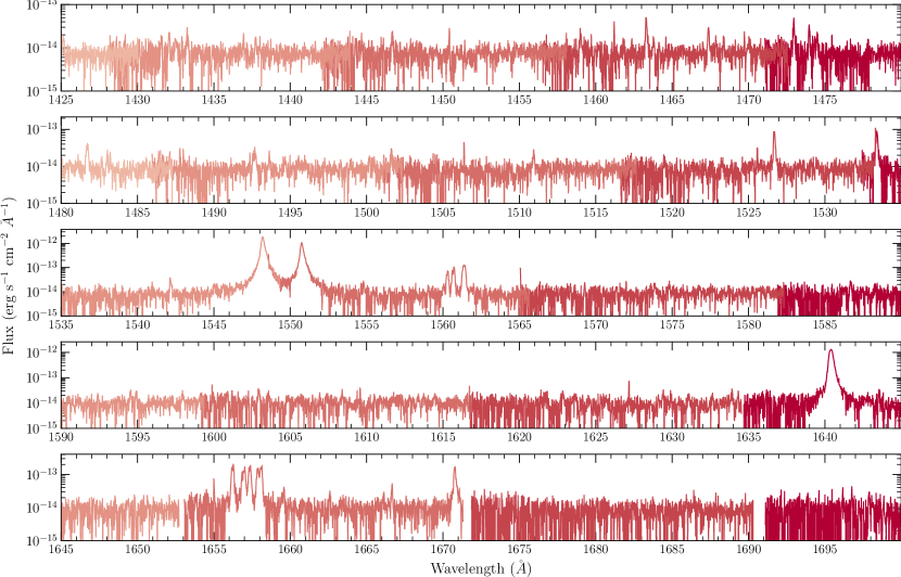
Figure 11: AU Mic’s quiescent spectrum – the last orbit from Visit 1.

HST/STIS

References

- Alam et al. (2018) Alam, M. K., Nikolov, N., López-Morales, M., et al. 2018, AJ, 156, 298
- Ben-Jaffel et al. (2022) Ben-Jaffel, L., Ballester, G. E., Muñoz, A. G., et al. 2022, Nature Astronomy, 6, 141
- Bourrier et al. (2015) Bourrier, V., Ehrenreich, D., & Lecavelier des Etangs, A. 2015, A&A, 582, A65
- Bourrier & Lecavelier des Etangs (2013) Bourrier, V., & Lecavelier des Etangs, A. 2013, A&A, 557, A124
- Bourrier et al. (2016) Bourrier, V., Lecavelier des Etangs, A., Ehrenreich, D., Tanaka, Y. A., & Vidotto, A. A. 2016, A&A, 591, A121
- Bourrier et al. (2018) Bourrier, V., Lecavelier des Etangs, A., Ehrenreich, D., et al. 2018, A&A, 620, A147
- Bourrier et al. (2022) Bourrier, V., Zapatero Osorio, M. R., Allart, R., et al. 2022, A&A, 663, A160
- Cale et al. (2021) Cale, B. L., Reefe, M., Plavchan, P., et al. 2021, AJ, 162, 295
- Carolan et al. (2020) Carolan, S., Vidotto, A. A., Plavchan, P., Villarreal D’Angelo, C., & Hazra, G. 2020, MNRAS, 498, L53
- Catling & Zahnle (2009) Catling, D. C., & Zahnle, K. J. 2009, Scientific American, 300, 36
- Chadney et al. (2015) Chadney, J. M., Galand, M., Unruh, Y. C., Koskinen, T. T., & Sanz-Forcada, J. 2015, Icarus, 250, 357
- Cohen et al. (2022) Cohen, O., Alvarado-Gómez, J. D., Drake, J. J., et al. 2022, ApJ, 934, 189
- Davenport et al. (2014) Davenport, J. R. A., Hawley, S. L., Hebb, L., et al. 2014, ApJ, 797, 122
- Del Zanna et al. (2021) Del Zanna, G., Dere, K. P., Young, P. R., & Landi, E. 2021, ApJ, 909, 38
- Dere et al. (1997) Dere, K. P., Landi, E., Mason, H. E., Monsignori Fossi, B. C., & Young, P. R. 1997, A&AS, 125, 149
- dos Santos et al. (2019) dos Santos, L. A., Ehrenreich, D., Bourrier, V., et al. 2019, A&A, 629, A47
- Duvvuri et al. (2023) Duvvuri, G. M., Pineda, J. S., Berta-Thompson, Z. K., France, K., & Youngblood, A. 2023, AJ, 165, 12
- Duvvuri et al. (2021) Duvvuri, G. M., Sebastian Pineda, J., Berta-Thompson, Z. K., et al. 2021, ApJ, 913, 40
- Ehrenreich et al. (2015) Ehrenreich, D., Bourrier, V., Wheatley, P. J., et al. 2015, Nature, 522, 459
- Feinstein et al. (2022) Feinstein, A. D., France, K., Youngblood, A., et al. 2022, AJ, 164, 110
- Foreman-Mackey et al. (2013) Foreman-Mackey, D., Hogg, D. W., Lang, D., & Goodman, J. 2013, Publications of the Astronomical Society of the Pacific, 125, 306
- Fossati et al. (2010) Fossati, L., Haswell, C. A., Froning, C. S., et al. 2010, ApJ, 714, L222
- Foster et al. (2022) Foster, G., Poppenhaeger, K., Ilic, N., & Schwope, A. 2022, A&A, 661, A23
- Fulton & Petigura (2018) Fulton, B. J., & Petigura, E. A. 2018, AJ, 156, 264
- Fulton et al. (2017) Fulton, B. J., Petigura, E. A., Howard, A. W., et al. 2017, AJ, 154, 109
- Gaia Collaboration et al. (2018) Gaia Collaboration, Brown, A. G. A., Vallenari, A., et al. 2018, A&A, 616, A1
- García Muñoz et al. (2021) García Muñoz, A., Fossati, L., Youngblood, A., et al. 2021, ApJ, 907, L36
- Gilbert et al. (2022) Gilbert, E. A., Barclay, T., Quintana, E. V., et al. 2022, AJ, 163, 147
- Ginzburg et al. (2018) Ginzburg, S., Schlichting, H. E., & Sari, R. 2018, MNRAS, 476, 759
- Gupta & Schlichting (2019) Gupta, A., & Schlichting, H. E. 2019, MNRAS, 487, 24
- Harbach et al. (2021) Harbach, L. M., Moschou, S. P., Garraffo, C., et al. 2021, ApJ, 913, 130
- Harris et al. (2020) Harris, C. R., Millman, K. J., van der Walt, S. J., et al. 2020, Nature, 585, 357. https://doi.org/10.1038/s41586-020-2649-2
- Haswell et al. (2012) Haswell, C. A., Fossati, L., Ayres, T., et al. 2012, ApJ, 760, 79
- Hawley et al. (2014) Hawley, S. L., Davenport, J. R. A., Kowalski, A. F., et al. 2014, ApJ, 797, 121
- Hoeijmakers et al. (2020) Hoeijmakers, H. J., Seidel, J. V., Pino, L., et al. 2020, A&A, 641, A123
- Hunter (2007) Hunter, J. D. 2007, Computing in science & engineering, 9, 90
- Jin et al. (2014) Jin, S., Mordasini, C., Parmentier, V., et al. 2014, ApJ, 795, 65
- Klein et al. (2021) Klein, B., Donati, J.-F., Moutou, C., et al. 2021, MNRAS, 502, 188
- Kramida et al. (2021) Kramida, A., Yu. Ralchenko, Reader, J., & and NIST ASD Team. 2021, NIST Atomic Spectra Database (ver. 5.9), [Online]. Available: https://physics.nist.gov/asd [2022, September 11]. National Institute of Standards and Technology, Gaithersburg, MD., ,
- Kreidberg (2015) Kreidberg, L. 2015, PASP, 127, 1161
- Kulow et al. (2014) Kulow, J. R., France, K., Linsky, J., & Loyd, R. O. P. 2014, ApJ, 786, 132
- Lannier et al. (2017) Lannier, J., Lagrange, A. M., Bonavita, M., et al. 2017, A&A, 603, A54
- Lavie et al. (2017) Lavie, B., Ehrenreich, D., Bourrier, V., et al. 2017, A&A, 605, L7
- Lecavelier Des Etangs (2007) Lecavelier Des Etangs, A. 2007, A&A, 461, 1185
- Lecavelier des Etangs et al. (2012) Lecavelier des Etangs, A., Bourrier, V., Wheatley, P. J., et al. 2012, A&A, 543, L4
- Lee & Connors (2021) Lee, E. J., & Connors, N. J. 2021, ApJ, 908, 32
- Lightkurve Collaboration et al. (2018) Lightkurve Collaboration, Cardoso, J. V. d. M., Hedges, C., et al. 2018, Lightkurve: Kepler and TESS time series analysis in Python, Astrophysics Source Code Library, , , ascl:1812.013
- Linsky et al. (2006) Linsky, J. L., Draine, B. T., Moos, H. W., et al. 2006, ApJ, 647, 1106
- Lopez & Fortney (2013) Lopez, E. D., & Fortney, J. J. 2013, ApJ, 776, 2
- Loyd & France (2014) Loyd, R. O. P., & France, K. 2014, ApJS, 211, 9
- Loyd et al. (2018a) Loyd, R. O. P., Shkolnik, E. L., Schneider, A. C., et al. 2018a, ApJ, 867, 70
- Loyd et al. (2018b) Loyd, R. O. P., France, K., Youngblood, A., et al. 2018b, ApJ, 867, 71
- Lundkvist et al. (2016) Lundkvist, M. S., Kjeldsen, H., Albrecht, S., et al. 2016, Nature Communications, 7, 11201
- Mamajek & Bell (2014) Mamajek, E. E., & Bell, C. P. M. 2014, MNRAS, 445, 2169
- Martioli et al. (2021) Martioli, E., Hébrard, G., Correia, A. C. M., Laskar, J., & Lecavelier des Etangs, A. 2021, A&A, 649, A177
- Mazeh et al. (2016) Mazeh, T., Holczer, T., & Faigler, S. 2016, A&A, 589, A75
- McCann et al. (2019) McCann, J., Murray-Clay, R. A., Kratter, K., & Krumholz, M. R. 2019, ApJ, 873, 89
- Nikolov et al. (2014) Nikolov, N., Sing, D. K., Pont, F., et al. 2014, MNRAS, 437, 46
- Owen (2022) Owen, J. 2022, in Bulletin of the American Astronomical Society, Vol. 54, 208.05
- Owen (2019) Owen, J. E. 2019, Annual Review of Earth and Planetary Sciences, 47, 67
- Owen & Alvarez (2016) Owen, J. E., & Alvarez, M. A. 2016, ApJ, 816, 34
- Owen & Lai (2018) Owen, J. E., & Lai, D. 2018, MNRAS, 479, 5012
- Owen & Wu (2013) Owen, J. E., & Wu, Y. 2013, ApJ, 775, 105
- Owen & Wu (2017) —. 2017, ApJ, 847, 29
- Owen et al. (2023) Owen, J. E., Murray-Clay, R. A., Schreyer, E., et al. 2023, MNRAS, 518, 4357
- Pagano et al. (2000) Pagano, I., Linsky, J. L., Carkner, L., et al. 2000, ApJ, 532, 497
- Plavchan et al. (2009) Plavchan, P., Werner, M. W., Chen, C. H., et al. 2009, ApJ, 698, 1068
- Plavchan et al. (2020) Plavchan, P., Barclay, T., Gagné, J., et al. 2020, Nature, 582, 497
- Powell et al. (1999) Powell, K. G., Roe, P. L., Linde, T. J., Gombosi, T. I., & De Zeeuw, D. L. 1999, Journal of Computational Physics, 154, 284
- Proffitt et al. (2017) Proffitt, C. R., Monroe, T., & Dressel, L. 2017, Status of the STIS Instrument Focus, Instrument Science Report STIS 2017-01 (v1), 30 pages, ,
- Raetz et al. (2020) Raetz, S., Stelzer, B., Damasso, M., & Scholz, A. 2020, A&A, 637, A22
- Riley et al. (2018) Riley, A., Monroe, T., & Lockwood, S. 2018, Impacts of focus on aspects of STIS UV Spectroscopy, Instrument Science Report STIS 2018-6, 25 pages, ,
- Rockcliffe et al. (2021) Rockcliffe, K. E., Newton, E. R., Youngblood, A., et al. 2021, AJ, 162, 116
- Rogers et al. (2021) Rogers, J. G., Gupta, A., Owen, J. E., & Schlichting, H. E. 2021, MNRAS, 508, 5886
- Rogers & Owen (2021) Rogers, J. G., & Owen, J. E. 2021, MNRAS, 503, 1526
- Schneider et al. (2019) Schneider, A. C., Shkolnik, E. L., Barman, T. S., & Loyd, R. P. 2019, ApJ, 886, 19
- Seidel et al. (2020) Seidel, J. V., Ehrenreich, D., Bourrier, V., et al. 2020, A&A, 641, L7
- Seidel et al. (2022) Seidel, J. V., Cegla, H. M., Doyle, L., et al. 2022, MNRAS, 513, L15
- Shaikhislamov et al. (2014) Shaikhislamov, I. F., Khodachenko, M. L., Sasunov, Y. L., et al. 2014, ApJ, 795, 132
- Sing et al. (2016) Sing, D. K., Fortney, J. J., Nikolov, N., et al. 2016, Nature, 529, 59
- Sing et al. (2019) Sing, D. K., Lavvas, P., Ballester, G. E., et al. 2019, AJ, 158, 91
- Stefànsson et al. (2022) Stefànsson, G., Mahadevan, S., Petrovich, C., et al. 2022, ApJ, 931, L15
- The Astropy Collaboration et al. (2018) The Astropy Collaboration, Price-Whelan, A. M., Sipőcz, B. M., et al. 2018, AJ, 156, 123
- Torres et al. (1972) Torres, C. A. O., Ferraz Mello, S., & Quast, G. R. 1972, Astrophys. Lett., 11, 13
- Tóth et al. (2012) Tóth, G., van der Holst, B., Sokolov, I. V., et al. 2012, Journal of Computational Physics, 231, 870
- Turnbull (2015) Turnbull, M. C. 2015, arXiv e-prints, arXiv:1510.01731
- Vidal-Madjar et al. (2003) Vidal-Madjar, A., Lecavelier des Etangs, A., Désert, J. M., et al. 2003, Nature, 422, 143
- Virtanen et al. (2020) Virtanen, P., Gommers, R., Oliphant, T. E., et al. 2020, Nature Methods
- White et al. (2019) White, R., Schaefer, G., Boyajian, T., et al. 2019, in American Astronomical Society Meeting Abstracts, Vol. 233, American Astronomical Society Meeting Abstracts #233, 259.41
- Wittrock et al. (2022) Wittrock, J. M., Dreizler, S., Reefe, M. A., et al. 2022, AJ, 164, 27
- Wyatt et al. (2020) Wyatt, M. C., Kral, Q., & Sinclair, C. A. 2020, MNRAS, 491, 782
- Yan et al. (2019) Yan, F., Casasayas-Barris, N., Molaverdikhani, K., et al. 2019, A&A, 632, A69
- Youngblood & Newton (2022) Youngblood, A., & Newton, E. R. 2022, allisony/lyapy: First release created for citation purposes in the literature, Zenodo, vv1.0.0, Zenodo, doi:10.5281/zenodo.6949067
- Youngblood et al. (2022) Youngblood, A., Pineda, J. S., Ayres, T., et al. 2022, ApJ, 926, 129
- Youngblood et al. (2016) Youngblood, A., France, K., Loyd, R. O. P., et al. 2016, ApJ, 824, 101
- Zhang et al. (2022a) Zhang, M., Knutson, H. A., Wang, L., et al. 2022a, AJ, 163, 68
- Zhang et al. (2022b) Zhang, Y., Snellen, I. A. G., Wyttenbach, A., et al. 2022b, A&A, 666, A47
- Zicher et al. (2022) Zicher, N., Barragán, O., Klein, B., et al. 2022, MNRAS, 512, 3060
- Zuckerman & Song (2004) Zuckerman, B., & Song, I. 2004, ARA&A, 42, 685