Learnability transitions in monitored quantum dynamics
via eavesdropper’s classical shadows

Abstract

Monitored quantum dynamics—unitary evolution interspersed with measurements—has recently emerged as a rich domain for phase structure in quantum many-body systems away from equilibrium. Here we study monitored dynamics from the point of view of an eavesdropper who has access to the classical measurement outcomes, but not to the quantum many-body system. We show that a measure of information flow from the quantum system to the classical measurement record—the informational power—undergoes a phase transition in correspondence with the measurement-induced phase transition (MIPT). This transition determines the eavesdropper’s (in)ability to learn properties of an unknown initial quantum state of the system, given a complete classical description of the monitored dynamics and arbitrary classical computational resources. We make this learnability transition concrete by defining classical shadows protocols that the eavesdropper may apply to this problem, and show that the MIPT manifests as a transition in the sample complexity of various shadow estimation tasks, which become harder in the low-measurement phase. We focus on three applications of interest: Pauli expectation values (where we find the MIPT appears as a point of optimal learnability for typical Pauli operators), many-body fidelity, and global charge in $U(1)$-symmetric dynamics. Our work unifies different manifestations of the MIPT under the umbrella of learnability and gives this notion a general operational meaning via classical shadows.

I Introduction

Recent advances in our ability to address and read out individual degrees of freedom in many-body quantum systems have motivated interest in new types of dynamics where the role of the observer is central. In these monitored dynamics Skinner et al. (2019); Li et al. (2018, 2019); Potter and Vasseur (2022); Fisher et al. (2022) the observer’s measurements shape the evolution of the system and drive it to sharply different possible ensembles of late-time states. These ‘measurement-induced phase transitions’ (MIPTs) thus define a new paradigm for phase structure in open systems away from equilibrium. At the same time, these technological developments have raised the salience of quantum state learning—the general problem of characterizing properties of unknown, potentially complex quantum states with as few measurements as possible Huang et al. (2020); Elben et al. (2023). In this work we connect these two threads by formulating MIPTs as learnability transitions within the framework of classical shadows, a leading practical approach to state learning.

The canonical formulation of the MIPT is in terms of a phase transition in the entanglement properties of ensembles of quantum trajectories Skinner et al. (2019); Li et al. (2018, 2019). In the standard setup, the system evolves through random circuit dynamics composed of local unitary gates interrupted by local projective measurements with probability $p$. As the measurement rate $p$ is tuned, the ensemble of late-time trajectories undergoes a phase transition from a disentangling phase in which trajectories display area-law entanglement (at high $p$, corresponding to frequent measurements) to an entangling phase in which trajectories display volume-law entanglement (at low $p$, corresponding to infrequent measurements). While the $p=0,1$ limits are transparent, the existence of a robust volume-law phase at any finite measurement rate is, a priori, surprising. While local unitary gates can only generate entanglement at the boundaries of a subsystem, disentangling measurements act everywhere in the bulk: a (naively) imbalanced competition which should always favor the area-law phase. A key insight for understanding the stability of the volume law phase was furnished in Refs. Choi et al. (2020); Gullans and Huse (2020a), which posited that the volume-law phase can be understood as a dynamically generated random code in which the correlations between two subsystems are highly non-local, and thus ‘hidden’ from local measurements. This naturally leads to two complementary information-theoretic perspectives on the MIPT: (a) the coding perspective and (b) the learning perspective, discussed below. The latter is the focus of this work.

Coding

The coding perspective is primarily understood from the point of view of an experimentalist, Alice, controlling a quantum system, see Fig. 1(a). Over the course of the dynamics, measurements are performed on the system (either by Alice herself or by a particular type of “environment” that broadcasts the measurement outcomes). These measurements disturb the initial state of the system. In order to undo this disturbance as much as possible, Alice can perform ‘recovery’ operations on the combined final state of the quantum system and classical measurement apparatus—concretely, she decodes the measurement record $\boldsymbol{m}$ (which is a binary string of measurement outcomes indexed by spacetime locations) to decide on a unitary operation $U_{\boldsymbol{m}}$ to apply to the quantum state. As a function of parameters in the monitored dynamics (typically the space-time density of measurements set by $p$), Alice’s ability to recover her initial state undergoes a phase transition: on the entangling side, she can successfully recover an extensive amount of quantum information; on the disentangling side, only a subextensive amount.

Figure 1: Different perspectives on measurement-induced phases of quantum information. (a) Coding perspective. A state $\rho$ of a quantum many-body system is subject to monitored dynamics, possibly after an encoding or “pre-scrambling” step (the global unitary $V$). The measurement record $\boldsymbol{m}$ stored in a classical system, here represented by the lab notebook. The experimentalist, Alice, has access to both the quantum and classical systems (green shaded box). After the dynamics, through classical computation conditioned on the measurement record $\boldsymbol{m}$, Alice finds a recovery operation $U_{\boldsymbol{m}}$ and applies it to the quantum system. There is a phase transition in how many qubits from the initial state $\rho$ can be recovered in this way, i.e. in the coding properties of monitored dynamics. (b) Learning perspective. An eavesdropper, Eve, has access only to the classical system (red shaded box). She attempts to learn properties of $\rho$ by estimating functions $f(\rho)$ (e.g. expectation values $\Tr(\rho O)$) via classical shadows. There is a phase transition in the sample complexity of these estimation tasks—i.e., in the learnability of the state $\rho$ from the measured data $\boldsymbol{m}$. The two perspectives (a,b) are dual to each other and the transitions coincide.

We refer to this point of view as the coding perspective on the MIPT Gullans and Huse (2020a); Choi et al. (2020), due to its close analogy with quantum error correction (QEC) Shor (1995); Gottesman (1997); Dennis et al. (2002). The measurement record $\boldsymbol{m}$ serves as the “syndrome” and the conditional unitary $U_{\boldsymbol{m}}$ as the correction / recovery operation; the MIPT arises as a phase transition in the rate of this code, i.e. the ratio of logical qubits to physical qubits, which goes from finite to vanishing. In other words, in the entangling phase an extensive amount of quantum information survives in the combined quantum-classical state of system and measurement record. While its recovery may be practically hard (in terms of classical computation and quantum circuit complexity), its in-principle presence or absence defines sharp phases. This corresponds to a a phase transition in the capacity of the channel that maps the initial quantum state to the combined quantum-classical post-measurement state Choi et al. (2020). This channel capacity also corresponds to the trajectory-averaged entropy of mixed states subject to the monitored evolution, so the coding transition is equally described as a dynamical purification transition Gullans and Huse (2020a). Further, the idea of decoding implicit in this setup has led to groundbreaking developments in our experimental understanding of the MIPT Gullans and Huse (2020b); Noel et al. (2022); Hoke et al. (2023).

Learning

In this work, we take a complementary perspective of learning rather than coding, i.e. we focus on the information transmitted to the classical measurement record alone, rather than the combined quantum-classical state. This perspective is centered on an “eavesdropper”, Eve, who does not have access to the quantum many-body system, but wants to learn some properties (e.g. observable expectation values) of its unknown initial state. She may try to do so by collecting classical measurement outcomes and performing suitable computation on them, Fig. 1(b).

This perspective has been studied in the literature in two contexts. The first studies the sensitivity of the distribution of measurement outcomes to changes in the initial state. In the second context, the monitored dynamics is enriched with a $U(1)$ symmetry, and an eavesdropper attempts to learn the global charge of a system from measurements of local charge densities Barratt et al. (2022a). In both cases, the focus is only on the information present in the classical measurement record, as the post-measurement quantum many-body state is considered inaccessible. This point of view is complementary to the coding perspective. An intituive expectation is that, if coding is successful, then the “syndrome” measurements $\boldsymbol{m}$ should reveal no infromation about the initial state, and thus learning should fail; conversely, if coding fails, information “leaks” into the classical measurement record and learning should become possible.

In this work we sharpen this intuition and make it operationally meaningful. We view the monitored dynamics as a single, complex “randomized measurement” Elben et al. (2023) performed on the system. From Eve’s point of view, this generalized measurement destroys the quantum state and turns it into classical data. As such, it is impossible for her to recover quantum information, as in coding (e.g., any entanglement with an outside reference system is destroyed in the process); but it may still be possible to learn a classical description of the state, as in tomography.

We introduce classical shadows protocols Huang et al. (2020) that Eve may use to learn various properties of the unknown initial state from the outcomes of many shots of these generalized measurements. We then show that the MIPT manifests as a transition in the sample complexity of these tasks, i.e. how many shots of the experiments Eve needs before she can confidently make predictions. The transition in sample complexity may be from polynomial to exponential, between two exponentials, or between two polynomials, depending on the task at hand. Our framework is very general and furnishes a unified language to describe and study learnability transitions in various different contexts (including previous examples from the literature such as charge learning Barratt et al. (2022a)). Finally, we argue, and prove in some cases, that these learnability transitions reflect a transition in the informational power Dall’Arno et al. (2011) of monitored dynamics—an intrinsic property independent of the chosen learning protocol.

The balance of this paper is structured as follows. In Sec. II we provide a concise, pedagogical review of relevant background topics: generalized measurements, monitored dynamics and classical shadows. Expert readers may safely skip this section. We then discuss monitored dynamics as a generalized measurement in Sec. III. We review the idea of informational power Dall’Arno et al. (2011) of generalized measurements and apply it to monitored dynamics, proving under certain assumptions (and conjecturing more generally) that it undergoes a phase transition at the MIPT. In Sec. IV we introduce “eavesdropper’s shadows”—classical shadows protocols that an eavesdropper may use to learn the state of the system from measurement records. The consequences of the MIPT on these classical shadows protocols are then analyzed in turn: Sec. V on the expectation value of Pauli operators, where we additionally investigate the effect of spatial locality on learnability; Sec. VI on many-body fidelities, which directly connects to recent work on the linear cross-entropy as an order parameter for the transition Li et al. (2023); and Sec. VII on learning properties of the charge distribution via $U(1)$-symmetric monitored dynamics Agrawal et al. (2022); Barratt et al. (2022a), which can also be studied naturally in the formalism of eavesdropper’s classical shadows. As we do not impose limits on classical computational resources, we find that the learnability transition coincides with the charge-sharpening transition in Ref. Agrawal et al. (2022), as expected Barratt et al. (2022a). Finally, in Sec. VIII we summarize our results and point out directions for future work.

II Review

In this Section we review essential background topics—generalized measurements (POVMs), monitored dynamics, and classical shadows—for the sake of a self-contained discussion. This part may be skipped by expert readers.

II.1 Generalized measurements

Generalized measurements in quantum mechanics are described by positive-operator-valued measures (POVMs), sets of operators $\{E_{\alpha}\}$ (also known as effects) that obey (i) positivity, $E_{\alpha}\geq 0$ and (ii) normalization $\sum_{\alpha}E_{\alpha}=\mathbb{I}$. These predict the probability of observing each outcome $\alpha$ on a given state $\rho$ by the identification $p_{\alpha}\equiv\Tr(\rho E_{\alpha})$, which is guaranteed to be a valid probability distribution by conditions (i-ii). A POVM describes measurement outcomes but not the associated post-measurement states of the quantum system. That additional data is contained in the instruments $\{K_{\alpha}\}$ (also known as Kraus operators in the context of quantum channels), that obey $E_{\alpha}=K_{\alpha}^{\dagger}K_{\alpha}$. The state $\rho$ is updated after the measurement as

$$\rho\mapsto\sum_{\alpha}p_{\alpha}\rho_{\alpha},\qquad\rho_{\alpha}=K_{\alpha}\rho K_{\alpha}^{\dagger}/p_{\alpha},$$ (1)

where $\rho_{\alpha}$ is the conditional post-measurement state of the system given outcome $\alpha$.

It may further be helpful to view the whole measurement process as a quantum-classical channel

$$\rho\mapsto\sum_{\alpha}p_{\alpha}\rho_{\alpha}\otimes\outerproduct{\alpha}{\alpha}_{C}$$ (2)

where the states $\outerproduct{\alpha}{\alpha}_{C}$ are states of a classical register, e.g. Alice’s lab notebook. We can always embed such states as orthonormal basis elements of a sufficiently large Hilbert space.

II.2 Monitored dynamics

Monitored dynamics is a type of open-system evolution whose quantum trajectories are labeled by a classical “measurement record” $\boldsymbol{m}$. We take $\boldsymbol{m}=(m_{t_{1},x_{1}},\dots m_{t_{M},x_{M}})\in\{0,1\}^{M}$ to be a collection of binary measurement outcomes gathered over different positions and times $(t_{i},x_{i})$ in the evolution. The quantum state $\rho$ evolves into a quantum-classical state

$$\rho\mapsto\sum_{\boldsymbol{m}}K_{\boldsymbol{m}}\rho K_{\boldsymbol{m}}^{\dagger}\otimes\outerproduct{\boldsymbol{m}}{\boldsymbol{m}}_{C},$$ (3)

which notably is of the same form as (2): we can in fact view the whole monitored evolution as a single POVM with $2^{M}$ possible outcomes $\boldsymbol{m}\in\{0,1\}^{M}$ occurring with probabilities $p_{\boldsymbol{m}}=\Tr(\rho E_{\boldsymbol{m}})$, $E_{\boldsymbol{m}}=K_{\boldsymbol{m}}^{\dagger}K_{\boldsymbol{m}}$.

Remarkably, it was discovered that the ensemble of quantum trajectories $\rho_{\boldsymbol{m}}\equiv K_{\boldsymbol{m}}\rho K_{\boldsymbol{m}}^{\dagger}/p_{\boldsymbol{m}}$ can undergo a sharp phase transition as a function of model parameters, e.g. the density or rate of measurements in the dynamics, from an “entangling” to a “disentangling” phase Potter and Vasseur (2022); Fisher et al. (2022); Skinner et al. (2019); Li et al. (2018, 2019); Choi et al. (2020); Bao et al. (2020); Gullans and Huse (2020a, b); Ippoliti et al. (2021); Lavasani et al. (2021a, b); Nahum et al. (2021); Li and Fisher (2021); Fan et al. (2021); Feng et al. (2022); Sierant et al. (2022); Koh et al. (2022); Noel et al. (2022); Hoke et al. (2023). The phenomenology of these phases is very rich and beyond the scope of this review section. Here we focus only on the aspect most relevant to this work, which is dynamical purification Gullans and Huse (2020a), closely related to the coding perspective discussed above: due to the non-unitarity of measurements, an initially-mixed state at late enough times generically becomes nearly pure, $\mathbb{E}_{\boldsymbol{m}}[\Tr(\rho_{\boldsymbol{m}}^{2})]\xrightarrow{t\to\infty}1$. Here the average is taken over the ensemble of trajectories with Born probability $p_{\boldsymbol{m}}=\Tr(\rho E_{\boldsymbol{m}})$. The time scale over which this happens varies sharply depending on which phase we are in: it is $O(\log(N))$ in the disentangling/pure phase, and $O(\exp(N))$ in the entangling/mixed phase. This reflects the emergence of a quantum code in the entangling phase, which protects some information and prevents it from leaking to the environment for very long times. In particular, taking a dynamic limit with $t,N\to\infty$ with $t=\Theta(N)$ ensures that the average purity becomes an order parameter for the two phases (1 in the disentangling phase, $<1$ in the entangling phase).

A subtle experimental aspect of this physics is that it is revealed only in nonlinear functions of the trajectories $\{\rho_{\boldsymbol{m}}\}$, such as the aforementioned average purity $\mathbb{E}_{\boldsymbol{m}}\Tr(\rho_{\boldsymbol{m}}^{2})$. It does not appear in the average of linear functions, which are fully determined by the average final density matrix $\rho^{\prime}=\mathbb{E}_{\boldsymbol{m}}[\rho_{\boldsymbol{m}}]=\sum_{\boldsymbol{m}}K_{\boldsymbol{m}}\rho K_{\boldsymbol{m}}^{\dagger}$. This is the output of dissipative dynamics and thus generically trivial across the phase diagram. A naïve approach based on measuring properties of individual trajectories incurs an exponential sampling overhead, $\sim 2^{M}$, due to postselection of the $M$ measurement outcomes (producing the same trajectory twice takes of order $2^{M}$ trials).

More sophisticated approaches that ameliorate or avoid this prohibitive sampling cost have been proposed Ippoliti and Khemani (2021); Ippoliti et al. (2022); Lu and Grover (2021); Gullans and Huse (2020b) and implemented experimentally Noel et al. (2022); Hoke et al. (2023). Ref. Gullans and Huse (2020b) proposed scalable order parameters that can be measured by decoding the measurement record and applying feedback control to the quantum system, similar to the setup in Fig. 1(a). Building on this, other approaches have more recently been proposed that bypass the need for quantum feedback by defining “hybrid” quantum-classical order parameters that correlate quantum state read-out with the output of classical simulations Dehghani et al. (2023); Garratt et al. (2023); Li et al. (2023); Hoke et al. (2023); Garratt and Altman (2023). These approaches generally trade the exponential sample complexity $\sim 2^{M}$ for the complexity of classical simulation, which may be polynomial or exponential depending on the models. We will show below that our work furnishes a new set of hybrid order parameters for the MIPT, in the form of variances of shadow estimators. We also note that another approach making use of classical shadows to diagnose the MIPT was proposed recently Garratt and Altman (2023), with the complementary goal of learning the final, post-measurement state. The goal is thus conceptually distinct from our learnability perspective, despite employing similar tools—a testament to the generality and wide applicability of the classical shadows framework, reviewed next.

II.3 Classical shadows

Classical shadows are a framework for learning properties of quantum states in a relatively sample-efficient manner by making use of randomized measurements Huang et al. (2020); Elben et al. (2023); Huang (2022); Struchalin et al. (2021); Chen et al. (2021); Levy et al. (2021); Kunjummen et al. (2023); Koh and Grewal (2022); Huang et al. (2021); Acharya et al. (2021); Nguyen et al. (2022); Wan et al. (2022); Hu et al. (2021); Akhtar et al. (2022); Bertoni et al. (2022); Arienzo et al. (2022); Ippoliti et al. (2023); Ippoliti (2023); Tran et al. (2023); McGinley and Fava (2022); Shivam et al. (2023). In this work we will make use of classical shadows in order to formulate a general framework that operationalizes the notion of “learnability” in monitored dynamics.

The standard shadows protocol Huang et al. (2020); Elben et al. (2023) attempts to learn properties of an unknown quantum state $\rho$ by making measurements in a complete orthonormal basis, e.g. the computational basis after a suitable random rotation $U$. From such a measurement one obtains a snapshot $\outerproduct{\boldsymbol{b}}{\boldsymbol{b}}$ of the rotated state $U\rho U^{\dagger}$, and thus a snapshot $U^{\dagger}\outerproduct{\boldsymbol{b}}{\boldsymbol{b}}U$ of the original state $\rho$ (here $\boldsymbol{b}\in\{0,1\}^{N}$ is an output bitstring). Averaging many such snapshots over outcomes of $\boldsymbol{b}$ and random choices of $U$ yields a “noisy” version of $\rho$:

$$\mathcal{M}(\rho)=\sum_{\boldsymbol{b}}\int{\rm d}U\,\bra{\boldsymbol{b}}U\rho U^{\dagger}\ket{\boldsymbol{b}}U^{\dagger}\outerproduct{\boldsymbol{b}}{\boldsymbol{b}}U,$$ (4)

where $\bra{\boldsymbol{b}}U\rho U^{\dagger}\ket{\boldsymbol{b}}$ is the probability of obtaining the measurement outcomes $\boldsymbol{b}$. Here ${\rm d}U$ is shorthand for whichever measure on the unitary group we are using (whether continuous or discrete) and $\mathcal{M}$ is known as the shadow channel. Therefore by “de-noising” our snapshots we obtain unbiased estimators of the true density matrix:

$$\hat{\rho}=\mathcal{M}^{-1}[U^{\dagger}\outerproduct{\boldsymbol{b}}{\boldsymbol{b}}U].$$ (5)

The classical simulation complexity of the protocol is determined by the complexity of obtaining the un-rotated snapshot $U^{\dagger}\outerproduct{\boldsymbol{b}}{\boldsymbol{b}}U$, and of determining and applying the inverse channel $\mathcal{M}^{-1}$ on a classical computer.

The snapshots in Eq. (5) can then be used to predict many properties of $\rho$; e.g. for linear expectation values $\langle O\rangle$, the estimators $\hat{o}=\Tr(\hat{\rho}O)$ average to the correct answer. The cost of the learning protocol is quantified by the number of samples that are needed to make an accurate prediction. This is dictated by the shadow norm $\|O\|_{\rm sh}^{2}$ (which controls the variance of $\hat{o}$), whose scaling depends on the chosen ensemble of measurements. Important results are known for the standard protocols based on local random Pauli (i.e. locally-randomized) and random Clifford (i.e. globally-randomized) measurements. In the former one has $\|P\|_{\rm sh}^{2}=3^{k}$ where $P$ is a Pauli operator of weight $k$, making the scheme practical for local (few-body) operators. In the latter, $\|O\|_{\rm sh}^{2}=\Tr(O^{\dagger}O)$ for any operator $O$, making the method suitable for low-rank operators such as pure-state projectors. This has the important application of computing many-body fidelity with pure states. The shadows protocol has recently been generalized to shallow shadows Akhtar et al. (2022); Bertoni et al. (2022); Arienzo et al. (2022); Ippoliti et al. (2023) in which the randomization step is effected by finite-depth circuits, and which yields an exponential gain in sampling complexity for the task of learning large, spatially contiguous $k$ body operators.

Classical shadows have been recently extended to the case of generalized (i.e. non-projective) measurements, represented by a POVM $\{E_{\alpha}\}$ Acharya et al. (2021); Nguyen et al. (2022) Given a measured outcome $\alpha$, there are several possibilities for what to use as a “snapshot”, giving rise to a family of shadow channels which generalize Eq. (4) and take the form

$$\mathcal{M}(\rho)=\sum_{\alpha}\int{\rm d}U\,\Tr(\rho E_{\alpha}^{U})\eta_{\alpha}^{U}.$$ (6)

Here we use the superscript $U$ to denote that the effect $E_{\alpha}$ and the snapshot $\eta_{\alpha}$ both in general depend on random unitary rotations that are part of the protocol, again represented by integration over ${\rm d}U$, but we do not assume a specific form. We will suppress this dependence on random unitaries from our notation in the following. In Sec. IV we will see three different choices for $\eta_{\alpha}$ that are well-motivated by conceptual or practical considerations.

III Informational power of monitored dynamics

Taking the learning perspective illustrated in Fig. 1(b), monitored dynamics as a whole is effectively a generalized measurement on the system—a process that maps the quantum state $\rho$ to a probability distribution over outcomes $\boldsymbol{m}$. In particular, if $K_{\boldsymbol{m}}$ is the evolution operator corresponding to trajectory $\boldsymbol{m}$, then the process is described by a POVM $\{E_{\boldsymbol{m}}\equiv K_{\boldsymbol{m}}^{\dagger}K_{\boldsymbol{m}}\}$ which maps the quantum state $\rho$ to the classical probability distribution $\{\Tr(\rho E_{\boldsymbol{m}})\}$. The question of learning thus boils down to the “strength” of this generalized measurement, or the information content of its outcomes.

To sharpen this notion, let us consider an ensemble of states $\mathcal{E}=\{(p_{i},\rho_{i})\}$. This is a discrete collection of states $\rho_{i}$, each one occurring with probability $p_{i}$, e.g. from some classical stochastic process involved in the state preparation. We want to know how well a POVM $\Pi=\{E_{\boldsymbol{m}}\}$ can distinguish the different states $\rho_{i}$ in the ensemble $\mathcal{E}$.

If the state $\rho_{i}$ was drawn, then the outcome $\boldsymbol{m}$ occurs with probability $p_{\boldsymbol{m}|i}\equiv\Tr(\rho_{i}E_{\boldsymbol{m}})$. Along with $p_{i}$ (given as part of the definition of $\mathcal{E}$), this defines the joint distribution

$$p_{i,\boldsymbol{m}}=p_{\boldsymbol{m}|i}p_{i}=\Tr(p_{i}\rho_{i}E_{\boldsymbol{m}})$$ (7)

and thus also the marginal $p_{\boldsymbol{m}}=\Tr(\rho E_{\boldsymbol{m}})$, with $\rho=\sum_{i}p_{i}\rho_{i}$ the average state of the ensemble. With this data, we can define the mutual information between the POVM $\Pi$ and the state ensemble $\mathcal{E}$ as the mutual information between variables $i$ and $\boldsymbol{m}$ in the joint distribution Eq. (7):

$$I(\mathcal{E}:\Pi) =-\sum_{i}p_{i}\ln p_{i}-\sum_{\boldsymbol{m}}p_{\boldsymbol{m}}\ln p_{\boldsymbol{m}}+\sum_{i,\boldsymbol{m}}p_{i,\boldsymbol{m}}\ln p_{i,\boldsymbol{m}}$$

$$=\sum_{i,\boldsymbol{m}}p_{i,\boldsymbol{m}}\ln\frac{p_{i,\boldsymbol{m}}}{p_{i}p_{\boldsymbol{m}}}$$ (8)

where the expression in the second line is in the form of a Kullback?Leibler divergence between the true distribution $p_{i,\boldsymbol{m}}$ and the product of its marginals $p_{i}p_{\boldsymbol{m}}$, in which the two variables are independent. Informally, this mutual information characterized how much the measurement outcome $\boldsymbol{m}$ knows about the underlying state $i$.

Finally, maximizing the mutual information $I(\mathcal{E}:\Pi)$ Eq. (8) over possible choices of the ensemble $\mathcal{E}$ yields an intrinsic property of the POVM $\Pi$ known as its informational power Dall’Arno et al. (2011); Dall’Arno (2014); Dall’Arno et al. (2014):

$$W(\Pi)=\max_{\mathcal{E}}I(\mathcal{E}:\Pi).$$ (9)

The optimization involved in the definition of informational power, Eq. (9), may be hard in general. However, it becomes trivial if we include a “pre-scrambling” or “encoding” step—meaning the system is rotated by a random unitary $V$ before being measured, as sketched in Fig. 1. In that case, we show in Appendix A that

$$W(\Pi)=Q(\mathbb{I}/D)-\sum_{\boldsymbol{m}}\pi_{\boldsymbol{m}}Q(\sigma_{\boldsymbol{m}}),$$ (10)

where $D$ is the Hilbert space dimension, $Q(\rho)$ is a function known as the subentropy (see Appendix A.2), and we have introduced a state ensemble $\mathcal{E}_{\Pi}=\{(\pi_{\boldsymbol{m}},\sigma_{\boldsymbol{m}})\}$ given by

$$\left\{\begin{aligned} &\pi_{\boldsymbol{m}}=\Tr(E_{\boldsymbol{m}})/D,\\ &\sigma_{\boldsymbol{m}}=E_{\boldsymbol{m}}/\Tr(E_{\boldsymbol{m}}).\end{aligned}\right.$$ (11)

This state ensemble is dual to our POVM $\Pi=\{E_{\boldsymbol{m}}\}$. It is straightforward to check, from the POVM conditions, that this is in fact a state ensemble, i.e. that $\pi_{\boldsymbol{m}}$ is a valid probability distribution and that the $\sigma_{\boldsymbol{m}}$ are states. In fact, both objects have intuitive physical interpretations: $\pi_{\boldsymbol{m}}$ is the probability of obtaining outcome $\boldsymbol{m}$ when running monitored dynamics on the fully-mixed state $\rho=\mathbb{I}/D$; $\sigma_{\boldsymbol{m}}\propto K_{\boldsymbol{m}}^{\dagger}(\mathbb{I}/D)K_{\boldsymbol{m}}$ is the output of Heisenberg-picture monitored evolution $K_{\boldsymbol{m}}^{\dagger}$, also acting on the fully-mixed state. In the most common models of monitored dynamics, made only of unitary gates and projective measurements Skinner et al. (2019); Li et al. (2018), the Schrödinger and Heisenber pictures are equivalent (at the ensemble level), so that we can interpret $\mathcal{E}_{\Pi}$ as a valid ensemble of trajectories for a monitored mixed-state evolution. Note that this is not the ensemble of physical monitored trajectories of the quantum system, $\{(p_{\boldsymbol{m}},K_{\boldsymbol{m}}\rho K_{\boldsymbol{m}}^{\dagger}/p_{\boldsymbol{m}})\}$, with $p_{\boldsymbol{m}}=\Tr(E_{\boldsymbol{m}}\rho)$: such states are inaccessible to Eve. The ensemble $\mathcal{E}_{\Pi}$ instead emerges as a description of the measurement process, built purely from a classical description of the dynamics (the $K_{\boldsymbol{m}}$ operators) available to Eve. This mapping of the measurement process to an auxiliary ensemble of monitored trajectories plays a key role in this work.

Having established this formalism, we can now interpret the analytical result for the informational power $W(\Pi)$, Eq. (10). An exact analytical expression for the subentropy $Q(\rho)$ in terms of the spectrum of $\rho$ is known Jozsa et al. (1994), but not particularly illuminating. However, for stabilizer states (in fact for all states proportional to projectors), one can analytically obtain a more explicit form for the subentropy (see Appendix A.3),

$$Q(\rho)=1-\gamma-\delta H(q^{S}).$$ (12)

Here $q$ is the local Hilbert space dimension ($D=q^{N}$), $S$ is the entropy of $\rho$ (in dits), $\gamma=0.577...$ is Euler-Mascheroni’s constant, and $\delta H(x)=H_{x}-(\ln(x)+\gamma)$ is the deviation of the harmonic sum $H_{x}=1+\frac{1}{2}+\dots+\frac{1}{x}$ from its large-$x$ expansion $\ln(x)+\gamma$. $\delta H$ is non-negative and bounded above by a constant; it vanishes as $\sim\frac{1}{2x}$ for large $x$.

Thus we arrive at the following result for monitored Clifford circuits (where all the trajectories $\sigma_{\mathbf{m}}$ are stabilizer states):

$$W(\Pi)=\mathbb{E}_{\mathbf{m}}[\delta H(q^{S_{\mathbf{m}}})]-\delta H(q^{N}),$$ (13)

with the average over trajectories taken according to the measure $\pi_{\mathbf{m}}$. This explicitly depends on the entropy of monitored trajectories $S_{\boldsymbol{m}}=-\log_{q}[\Tr(\sigma_{\boldsymbol{m}}^{2})]$, meaning that the dynamical purification transition manifests as a transition in the informational power. In the entangling phase, the trajectories $\sigma_{\boldsymbol{m}}$ remain highly mixed, with $S_{\boldsymbol{m}}\propto N$; for large $N$, employing the expansion $\delta H(x)\sim 1/(2x)$, we obtain

$$W(\Pi)\simeq\frac{1}{2}\mathbb{E}_{\mathbf{m}}[\Tr(\sigma_{\boldsymbol{m}}^{2})]-\frac{1}{2D}\xrightarrow{D\to\infty}0,$$ (14)

so that the informational power, which quantifies learnability from the measurement record, goes to zero in the entangling phase. In the disentangling phase, the trajectories purify and the entropies $S_{\boldsymbol{m}}$ quickly decay towards zero (reaching $O(1)$ values at logarithmic depth) and thus $\delta H(q^{S_{\boldsymbol{m}}})$ remains finite.

To summarize, we have shown that the informational power of pre-scrambled Clifford monitored dynamics of depth $t={\rm poly}(N)$ for large systems $N\gg 1$ obeys

$$W(\Pi)=\left\{\begin{aligned} &\sim q^{-sN}&\text{ (entangling phase)},\\ &\textsf{const.}>0&\text{ (disentangling phase)},\end{aligned}\right.$$ (15)

with $s\in[0,1]$ the order parameter of the purification phase transition (entropy density). We conjecture that the same transition holds for generic (non-Clifford) monitored dynamics. A suggestive result to this effect is that a Renyi-2 version of the mutual information $I(\mathcal{E}:\Pi)$ can be computed exactly and depends only on the average purity of the system, thus manifestly displaying the purification transition (see Appendix A.4). While this is not a valid mutual information, in randomized settings it is often a good proxy for the qualitative behavior of the true mutual information.

We note that the informational power is related to the Fisher information diagnostic in Ref. Bao et al. (2020) which measures the susceptibility of the measurement outcome distribution to small changes in the initial state. Like the informational power, the Fisher information aims to quantify how much information about the quantum state flows into the measurement record, thus the two approaches are closely related. A technical difference is that the Fisher information depends on the initial state and the choice of perturbation, while the informational power is an intrinsic property of the monitored dynamics. More importantly, the Fisher information diagnostic in Ref. Bao et al. (2020) generically requires the collection of exponentially many samples (so that probability distributions can be estimated with some accuracy), while in our work we will show that the transition in informational power is reflected in the complexity of classical shadows, and can be determined from few samples—the complexity bottleneck in our scheme lies instead in the classical simulation of the quantum system (needed to carry out classical shadow estimation).

Finally, we note that the informational power is equal to the channel capacity of the quantum-to-classical channel mapping the state $\rho$ to a classical probability distribution over measurement records $\boldsymbol{m}$ Dall’Arno et al. (2011): $\rho\mapsto\sum_{\mathbf{m}}\Tr(E_{\boldsymbol{m}}\rho)\outerproduct{\mathbf{m}}{\mathbf{m}}_{C}$, where $\{\ket{\mathbf{m}}_{C}\}$ is an orthonormal basis of classical states of the measurement device, as in Eq. (3). Therefore $W(\Pi)$ directly quantifies the flow of information from Alice’s unknown state to Eve’s classical data, sketched in Fig. 1(b). The MIPT arises as a sharp transition in this flow of information. In the rest of this work we examine how this transition affects Eve’s ability to learn properties of the quantum state $\rho$.

IV Eavesdropper’s shadows

The informational power transition discussed above suggests a general characterization of the MIPT as a learnability phase transition. To assign an operational meaning to the transition, one needs to consider concrete protocols that Eve might employ to learn features of Alice’s unknown initial state $\rho$ from the eavesdropped classical data $\mathbf{m}$. Classical shadows, reviewed in Sec. II.3, have emerged as a general and powerful framework for addressing this type of problem. Here we apply them to the generalized measurement associated with monitored dynamics. We will refer to these protocols as “eavesdropper’s shadows”.

IV.1 Setup

We consider an experimentalist, Alice, who controls a quantum many-body system, and an eavesdropper, Eve, who wants to learn properties of Alice’s system without having access to it. Alice prepares an initial state $\rho$ and runs some model of monitored dynamics on it (e.g. a brickwork circuit with single-qubit projective measurements Skinner et al. (2019); Li et al. (2018)). She iterates this process many times, with the same state $\rho$ but a different realization of the dynamics each time. Eve only has access to the following, purely classical data, for each run of the experiment:

1. complete classical description of the monitored dynamics (e.g. circuit architecture, gates, locations and basis of measurements);

2. mid-circuit measurement record $\boldsymbol{m}$.

Eve aims to learn as much as she can about the initial state $\rho$ from as few runs of the experiment as possible. This setup in sketched in Fig. 1(b).

Eve’s task can be readily cast in the framework of classical shadows with generalized measurements Acharya et al. (2021); Nguyen et al. (2022). From Eve’s point of view, this setup is equivalent to a generalized measurement of $\rho$, namely the POVM $\Pi=\{E_{\boldsymbol{m}}=K_{\boldsymbol{m}}^{\dagger}K_{\boldsymbol{m}}\}$, with $K_{\boldsymbol{m}}$ being the Kraus operator for quantum trajectory $\boldsymbol{m}$ of the monitored dynamics. While we have left it implicit to lighten our notation, $E_{\boldsymbol{m}}$ also depends on random unitary gates that vary with each realization; therefore, it is a type of randomized measurement Elben et al. (2023). The problem of learning about $\rho$ from outcomes $\boldsymbol{m}$ of the randomized measurements is thus formally analogous to the standard classical shadows protocol Huang et al. (2020); Elben et al. (2023), Sec. II.3.

IV.2 Protocol

In the standard protocol, based on a projective POVM $\{U^{\dagger}\outerproduct{\boldsymbol{b}}{\boldsymbol{b}}U\}$, the choice of a post-measurement “snapshot” state is automatic—upon getting outcome $\boldsymbol{b}$, the best guess for the pre-measurement state is just the POVM element itself, $\sigma_{U,\boldsymbol{b}}\equiv U^{\dagger}\outerproduct{\boldsymbol{b}}{\boldsymbol{b}}U$. In the general case, with a non-projective POVM $\{E_{\boldsymbol{m}}\}$, the choice is less obvious. In fact, there are several valid choices motivated on practical or conceptual grounds, as we will see below; all of them recover the “canonical” choice in the limit of the POVM becoming projective. Denoting a choice of snapshot state by $\eta_{\boldsymbol{m}}$, we have a measure-and-prepare channel

$$\mathcal{M}(\rho)=\sum_{\mathbf{m}}\Tr(E_{\boldsymbol{m}}\rho)\eta_{\mathbf{m}}$$ (16)

which can in principle be used for classical shadow estimation, along the same steps outlined in Sec. II.3.

A natural choice for $\eta_{\boldsymbol{m}}$ is based on a general mapping between POVMs and state ensembles, Eq. (11): we propose setting $\eta_{\boldsymbol{m}}=\sigma_{\boldsymbol{m}}$. This choice closely mirrors the standard protocol, Sec. II.3, upon replacing $U\mapsto K_{\boldsymbol{m}}$ (random monitored dynamics instead of random unitary rotation) and $\outerproduct{\boldsymbol{b}}{\boldsymbol{b}}\mapsto\mathbb{I}/D$. The latter is a uniform average over all possible outcomes $\ket{\boldsymbol{b}}$, representing Eve’s complete ignorance about the final state of the system. Beyond this heuristic reasoning, we note that this choice can be formally motivated as the Petz recovery map Petz (1986); Barnum and Knill (2002); Wilde (2015); Penington et al. (2022) from the space of measurement records to the space of quantum states, see App. B.

With this prescription, the shadow channel reads

$$\mathcal{M}(\rho) =\sum_{\boldsymbol{m}}\Tr(\rho E_{\boldsymbol{m}})\sigma_{\boldsymbol{m}}$$

$$=D\sum_{\boldsymbol{m}}\pi_{\boldsymbol{m}}\Tr(\rho\sigma_{\boldsymbol{m}})\sigma_{\boldsymbol{m}}$$

$$=D\Tr_{2}[(\mathbb{I}\otimes\rho)\sigma^{(2)}],$$ (17)

where ${\rm Tr}_{2}$ is the partial trace over the second replica, and $\sigma^{(2)}$ is the second moment operator of the state ensemble $\mathcal{E}_{\Pi}=\{(\pi_{\boldsymbol{m}},\sigma_{\boldsymbol{m}})\}$ dual to our POVM $\Pi=\{E_{\boldsymbol{m}}\}$ [see Eq. (11)]:

$$\sigma^{(2)}=\sum_{\boldsymbol{m}}\pi_{\boldsymbol{m}}\sigma_{\boldsymbol{m}}^{\otimes 2}.$$ (18)

For most typical models of monitored dynamcs (featuring only unitary evolution and projective measurements), the states $\sigma_{\boldsymbol{m}}$ are quantum trajectories of a valid monitored evolution $K_{\boldsymbol{m}}^{\dagger}$ acting on the fully-mixed state; thus the second-moment operator $\sigma^{(2)}$ is directly sensitive to the MIPT. For instance the order parameter of dynamical purification phases Gullans and Huse (2020a, b) (Sec. II.2), the trajectory-averaged purity $\mathcal{P}$, can be obtained as an expectation value on the two-replica state $\sigma^{(2)}$:

$$\mathcal{P}=\sum_{\boldsymbol{m}}\pi_{\boldsymbol{m}}\Tr(\sigma_{\boldsymbol{m}}^{2})=\Tr(\sigma^{(2)}\hat{\tau}),$$ (19)

with $\hat{\tau}$ the replica SWAP operator. Thus $\sigma^{(2)}$ undergoes a sharp change at the MIPT, and by extension so does the shadow channel $\mathcal{M}$, Eq. (17). We will investigate the consequences of this sharp change in terms of learnability transitions in the rest of the manuscript.

IV.3 Alternative prescriptions

Before proceeding, we note that other choices for the “snapshot” $\eta_{\mathbf{m}}$ are possible and well-motivated. In particular, two choices have been considered in the literature in the context of classical shadows with generalized measurements Acharya et al. (2021); Nguyen et al. (2022). We discuss them in detail in Appendix B, and briefly summarize the results below:

• Least squares Nguyen et al. (2022): set $\eta_{\boldsymbol{m}}=E_{\boldsymbol{m}}$. This is not a state (due to trace normalization), and the resulting “shadow channel” $\mathcal{M}(\rho)=\sum_{\boldsymbol{m}}\Tr(\rho E_{\boldsymbol{m}})E_{\boldsymbol{m}}$ is thus not a channel. Classical shadows work regardless. This choice minimizes the two-norm distance between the observed ($\Tr(\rho E_{\boldsymbol{m}})$) and predicted ($\Tr(\hat{\rho}E_{\boldsymbol{m}})$, with $\hat{\rho}$ the classical shadow of $\rho$) measurement outcome distributions. The shadow channel takes a form analogous to Eq. (17) [see Eq. (85)], but with a modified second-moment operator

  $$\tilde{\sigma}^{(2)}=\sum_{\boldsymbol{m}}\tilde{\pi}_{\boldsymbol{m}}\sigma_{\boldsymbol{m}}^{\otimes 2}$$ (20)

  where the probabilities are $\tilde{\pi}_{\boldsymbol{m}}=\pi_{\boldsymbol{m}}^{2}/\sum_{\boldsymbol{m}^{\prime}}\pi_{\boldsymbol{m}^{\prime}}^{2}$. This also features a MIPT, albeit with a different universality class due to a different reweighting of the trajectories Bao et al. (2020); Vasseur et al. (2019); Jian et al. (2020); Bao et al. (2021); Li et al. (2023).

• Maximum fidelity Acharya et al. (2021): set $\eta_{\boldsymbol{m}}=\outerproduct{\psi_{\boldsymbol{m}}}{\psi_{\boldsymbol{m}}}$ where $\ket{\psi_{\boldsymbol{m}}}$ is the leading eigenvector of $E_{\boldsymbol{m}}$ (we neglect degeneracies). This choice maximizes the fidelity $\bra{\phi}\mathcal{M}(\outerproduct{\phi}{\phi})\ket{\phi}$ between the input and output of $\mathcal{M}$, on average over Haar-random input states $\ket{\phi}$. Again the shadow channel takes a form analogous to Eq. (17) [see Eq. (88)], but with $\sigma^{(2)}$ replaced by the state

  $$\sigma^{(\infty,1)}=\sum_{\boldsymbol{m}}\pi_{\boldsymbol{m}}\outerproduct{\psi_{\boldsymbol{m}}}{\psi_{\boldsymbol{m}}}\otimes\sigma_{\boldsymbol{m}}.$$ (21)

  The expectation of the replica SWAP $\hat{\tau}$ on this state yields the average of $q^{-S_{\infty}}$, meaning this is also sensitive to the MIPT (with the same universality and critical point as Eq. (17) in this case).

We note that all three prescriptions reduce to the one from Ref. Huang et al. (2020) for the case of projective measurements, but they differ for generalized measurements. In the following we will use the prescription $\eta_{\boldsymbol{m}}=\sigma_{\boldsymbol{m}}$ unless otherwise specified; the qualitative conclusions would be unchanged with either prescription, since as we saw each of them is sensitive to the MIPT.

To summarize, we have examined different strategies that Eve might use to learn properties of Alice’s unknown initial state $\rho$ from the measurement record $\boldsymbol{m}$ via classical shadows. We have found that the shadow channel is determined by a moment operator for an emergent ensemble of monitored quantum trajectories of a mixed-state dynamics, Eq. (11). As the second moment of trajectories is sensitive to the MIPT, we expect this to lead to a qualitative change in the performance of classical shadows. In the following sections we work out the consequences of this observation on a range of different manifestations of the measurement-induced phase transition. Our results are schematically summarized in Fig. 2.

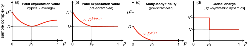
Figure 2: Schematic summary of main results for the sample complexity of various estimation tasks via “eavesdropper’s shadows”, as a function of the measurement rate $p$. $N$ is the system size, $D=q^{N}$ is the Hilbert space dimension, and $s(p)$ is the entropy density (order parameter of the entangling phase). (a) Estimation of Pauli expectation values, Sec. V.2. Different operators have different complexity; the curve shows the qualitative behavior of average or typical elements of the $N$-qudit Pauli group. The MIPT ($p=p_{c}$) emerges as a point of minimum complexity. (b) Estimation of Pauli expectation values with a pre-scrambling step, Sec. V.3. All non-identity Paulis have the same complexity, $\sim D^{1+s(p)}$, which changes non-analytically at the MIPT. (c) Estimation of many-body fidelity (with a pre-scrambling step), Sec. VI. The complexity transitions from constant to exponential in $N$ at the MIPT. (d) Estimation of global charge from dynamics with $U(1)$ symmetry, Sec. VII. The complexity transitions from $\sim N$ to $\sim N^{2}/t$ at the charge-sharpening transition, $p=p_{\#}$.

V Learning Pauli expectation values

In this section we begin to unravel the consequences of the connection between “eavesdropper’s shadows” and dynamical purification of mixed states introduced in Sec. IV. We start by focusing on Eve’s ability to learn Pauli expectation values on the unknown initial state $\rho$, namely to estimate $\langle P\rangle=\Tr(\rho P)$ ($P$ is a Pauli operator) to constant additive error $\epsilon$.

V.1 Shadow norm and entanglement

In general, the sample complexity of learning the expectation of an operator $O$ on a state $\rho$ is given by its squared shadow norm $\|O\|_{\rm sh}^{2}$, see Sec. II.3. This is given formally by

$$\|O\|_{\rm sh}^{2}=D\Tr(\rho\otimes\mathcal{M}^{-1}(O)\otimes\mathcal{M}^{-1}(O)\,{\sigma^{(3)}}),$$ (22)

where ${\sigma^{(3)}}=\sum_{\mathbf{m}}\pi_{\mathbf{m}}\sigma_{\mathbf{m}}^{\otimes 3}$ is the third moment operator of the trajectory ensemble $\mathcal{E}=\{(\pi_{\boldsymbol{m}},\sigma_{\boldsymbol{m}})\}$. If the ensemble is Pauli-invariant Hu et al. (2021); Bu et al. (2022) and $O$ is a Pauli operator, Eq. (22) simplifies to

$$\|O\|_{\rm sh}^{2}=\frac{1}{D}\Tr(O\mathcal{M}^{-1}(O)),$$ (23)

which is independent of $\rho$. Furthermore, if the POVM is invariant under multiplication by single-site Pauli operators Bu et al. (2022) (as is the case in typical models of monitored dynamics, made with random Haar or Clifford gates), the Pauli operators are eigenmodes of the channel: $\mathcal{M}(P)=\lambda_{P}P$. Thus, by Eq. (23), their shadow norm is $\|P\|_{\rm sh}^{2}=\lambda_{P}^{-1}$.

We now derive a relationship between the eigenvalues $\lambda_{P}$ (controlling the shadow norms of Pauli operators) and the entanglement structure of the ensemble of trajectories $\mathcal{E}$. We have, using operator-to-state notation [$(O|$ for super-bras, $|O)$ for super-kets, with inner product $(A|B)=\Tr(A^{\dagger}B)$],

$$\lambda_{P}=\frac{(P|\mathcal{M}|P)}{(P|P)}=\Tr[P^{\otimes 2}\sigma^{(2)}].$$ (24)

At the same time, the averaged purity of a subsystem $A$ in the ensemble of monitored trajectories $\mathcal{E}$ is

$$\mathcal{P}_{A}=\Tr[\hat{\tau}_{A}\sigma^{(2)}]$$ (25)

with $\hat{\tau}_{A}$ the replica SWAP operator acting only on subsystem $A$. We can expand $\hat{\tau}$ in the Pauli basis as

$$\hat{\tau}_{A}=\frac{1}{D_{A}}\sum_{P:\,{\sf supp}(P)\subseteq A}P^{\otimes 2},$$ (26)

where $D_{A}$ is the Hilbert space dimension for subsystem $A$ and $\textsf{supp}(P)$ denotes the support of $P$, i.e. the subsystem where $P$ is non-identity. A relationship between the entanglement feature $\{\mathcal{P}_{A}\}$ and the eigenvalues $\{\lambda_{A}\}$ of channel $\mathcal{M}$ follows:

$$D_{A}\mathcal{P}_{A}=\sum_{P:\,{\sf supp}(P)\subseteq A}\lambda_{P}=\sum_{B\subseteq A}(q^{2}-1)^{|B|}\lambda_{B},$$ (27)

where the first sum is over Pauli operators $P$ supported inside $A$, while the second is over subsystems $B$ contained inside $A$. The second equality holds because there are $(q^{2}-1)^{|B|}$ distinct Pauli operators with support $B$. The inverse of Eq. (27) yields

$$\lambda_{A} =(1-q^{2})^{-|A|}\sum_{B\subseteq A}\mathcal{P}_{B}(-q)^{|B|},$$ (28)

which is a well-known relationship between entanglement and shadow norm in the theory of classical shadows Hu et al. (2021); Akhtar et al. (2022); Bu et al. (2022); Ippoliti et al. (2023); Ippoliti (2023); we see that it straightforwardly extends to our setting of shadows with generalized measurements, when taking $\{\mathcal{P}_{A}\}$ to be the entanglement feature of monitored trajectories $\sigma_{\boldsymbol{m}}$.

Eq. (27) and (28) connect entanglement properties of the trajectories with shadow norms of Pauli operators. This is interesting as it suggests a sharp change in the performance of classical shadows at the dynamical purification transition, consistent with our prior analysis in Sec. III and IV. The connection between entanglement and shadow norms in Eq. (28) is not straightforward, as it is a sum of exponentially many terms with alternating signs. Nonetheless, a simple exact statement can be made about the harmonic mean of $\|P\|_{\rm sh}^{2}$ for all Pauli operators supported inside a subsystem $A$: rewriting Eq. (27), we have

$$\left(\frac{1}{D_{A}^{2}}\sum_{P:\,{\sf supp}(P)\subseteq A}\|P\|_{\rm sh}^{-2}\right)^{-1}=D_{A}/\mathcal{P}_{A}\sim D_{A}^{1+s},$$ (29)

where $s\in[0,1]$ is an entropy density defined by the scaling of average purity $\mathcal{P}_{A}\sim q^{-sN_{A}}=D_{A}^{-s}$. This implies a sharp change of the shadow norm distribution at the purification transition, which separates the pure phase ($s=0$) from the mixed phase ($s>0$). The harmonic mean of squared shadow norms scales exponentially in subsystem size $N_{A}$ on both sides of the transition, but the coefficient in the exponential changes non-analytically from $\sim q^{N_{A}}$ to $\sim q^{(1+s)N_{A}}$. Notably, the harmonic mean Eq. (29) is a lower bound to both the average shadow norm (arithmetic mean) and the typical shadow norm (geometric mean), implying that both must diverge as $\Omega(2^{(1+s)N_{A}})$ in the entangling phase and as $\Omega(2^{N_{A}})$ in the disentangling phase.

V.2 Optimal learning at the MIPT

To gain more insight on the structure of the shadow norm distribution, beyond the exact harmonic-mean result of Eq. (29) and the bounds it implies, we turn to numerical simulations. We perform exact numerical simulations of mixed-state monitored dynamics (a standard model made of brickwork layers of Haar-random gates and single-qubit $Z$ measurements with probability $p\in[0,1]$) on up to $L=14$ qubits. Note we are limited to this size by the fact that we simulate mixed-state dynamics. We obtain the entanglement feature $\{\mathcal{P}_{A}\}$ averaged over many realizations of the dynamics; from the entanglement feature we obtain the full set of shadow norms $\{\lambda_{A}^{-1}\}$ via Eq. (28). Results are shown in Fig. 3. The harmonic mean of shadow norms, as predicted, is a function only of the averaged purity, and is thus monotonically decreasing in the measurement rate $p$. However the arithmetic mean $D^{-2}\sum_{P}\|P\|_{\rm sh}^{2}$ exhibits non-monotonic behavior, with a minimum near the purification transition $p\approx 0.16$.

This is explained by the fact that, deep in the pure phase, one recovers random Pauli shadows (i.e. shadows with random local, single-qubit Pauli measurements). This is exactly true at $p=1$, and we expect it to be a fairly accurate approximation throughout $p\geq 0.5$, where the circuit is non-percolating. In this regime, even with complete access to the system, spatial locality makes learning large Pauli operators very inefficient. On the other hand, in the mixed phase, as seen earlier, the informational power of Eve’s measurements goes to zero, making any learning inefficient. The MIPT is a “sweet spot” between these two obstructions: the informational power is still finite (at polynomial depth), while the restriction of locality is alleviated.

Throughout the area-law phase, we expect eavesdropper’s shadows to perform similarly to shallow shadows Akhtar et al. (2022); Bertoni et al. (2022); Arienzo et al. (2022); Ippoliti et al. (2023) with finite depth: i.e., Eve manages to eventually read out all the information, but this takes an amount of time that grows as the transition is approached, giving information more time to spread, analogous to increasing circuit depth in shallow shadows. At the transition, this “effective depth” should diverge; it is tempting to speculate a relationship with shallow shadows at $\log(N)$ depth, which were shown to give Pauli shadow norms $\sim q^{N}$ for large Pauli operators (consistent with the scaling of both harmonic and arithmetic-mean $\|P\|_{\rm sh}^{2}$ at the MIPT observed here).

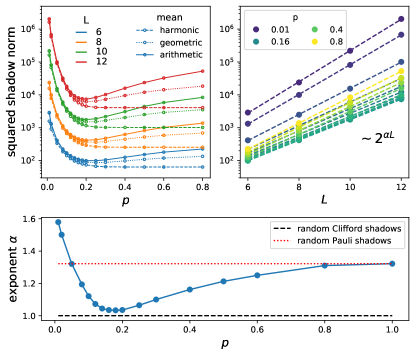
Figure 3: (a) Squared shadow norms of Pauli operators under eavesdropper’s shadows as a function of measurement rate $p$, for different system sizes $N$: the harmonic mean (dotted lines) is monotonically-decreasing in $p$, being completely fixed by the system’s purity; the arithmetic mean (solid lines) shows a minimum at the MIPT. (b) Same data (for the arithmetic mean) plotted as a function of $N$ displays clear exponential scaling $\sim D^{\alpha}=2^{\alpha N}$. Dashed lines are fits. (c) Fit coefficient $\alpha$ vs $p$ shows a minimum at the MIPT.

Thus there are two conceptually-independent reasons why Eve’s task of learning the expectation values of general Pauli operators via classical shadows may be hard: spatial locality at large $p$ (pure/disentangling phase) and a fundamental lack of information at large $p$ (entangling/mixed/coding phase). Numerical results indicate that an optimum is reached near the purification transition, $p_{c}\approx 0.16$, where the performance is close to random Clifford shadows ($\|P\|_{\rm sh}^{2}\sim D$ for all traceless $P$). This is a novel characterization of the MIPT, as the optimum rate $p$ for learning Pauli expectation values from the measurement record.

V.3 Complexity transition

For the rest of this work, we will focus on the presence or absence of any information in the measurement record, regardless of its locality structure. For this reason, it is advantageous to “pre-scramble” the input state $\rho$ with a random global Clifford operation $V$, as in Sec. III, which eliminates issues with spatial locality. This dramatically simplifies the picture, as the channel $\mathcal{M}$ now depends on a single property of the trajectory ensemble—its average global purity $\mathcal{P}$. We have

$$\mathcal{M}(\rho) =D\int{\rm d}V\,\Tr_{2}[(\mathbb{I}\otimes\rho)\,V^{\otimes 2}\sigma^{(2)}(V^{\dagger})^{\otimes 2}]$$

$$=\frac{(D-\mathcal{P})\Tr(\rho)\mathbb{I}+(D\mathcal{P}-1)\rho}{D^{2}-1}$$ (30)

This reproduces the familiar random-Clifford result $(\mathbb{I}+\rho)/(D+1)$ for $\mathcal{P}=1$. For $\mathcal{P}=1/D$ (no measurements), it correctly gives $\mathbb{I}/D$: there is no information at all about $\rho$, the measurement channel is a global erasure and is not invertible. Intermediate values of $\mathcal{P}$ interpolate between these two extremes. In particular the channel is invertible whenever $\mathcal{P}>1/D$.

It follows that all traceless operators are eigenmodes of $\mathcal{M}$ with eigenvalue

$$\lambda=\frac{D\mathcal{P}-1}{D^{2}-1}=\frac{D^{1-s}-1}{D^{2}-1}\sim D^{-(1+s)}$$ (31)

where $\sim$ denotes asymptotic scaling at large $D$. Thus in particular, all Pauli operators $P\neq I$ have shadow norm

$$\|P\|_{\rm sh}^{2}\sim D^{1+s}=q^{(1+s)N}$$ (32)

which indeed changes sharply at the purification transition, as the entropy density goes from $s=0$ (pure phase) to $s>0$ (mixed phase).

V.4 Information extracted per measurement

The result in Eq. (32) implies that, to learn the expectation of $P$ on the unknown state $\rho$, Eve needs many more samples in the mixed phase than she does in the pure phase—a factor of $\sim q^{sN}$ more. In other words, the amount of information about $\rho$ leaking into the measurement record $\boldsymbol{m}$ is suppressed exponentially in the mixed phase. This characterization of the mixed or coding phase Choi et al. (2020); Gullans and Huse (2020a, b) is complementary to the exponentially-long lifetime (also $\sim q^{sN}$) of information in the system.

In the present framework, however, we can make an even more precise statement about the way in which information on $\rho$ leaks into the measurement record. A key result in dynamical purification Gullans and Huse (2020a); Li and Fisher (2021) is that, as a function of circuit depth $t$, the entropy density $s$ in the mixed phase decreases as

$$s(t)\sim s_{0}-\frac{1}{N}\log_{q}(t)$$ (33)

(at times $1\ll t\ll q^{s_{0}N}$), where $s_{0}$ is the entropy density “plateau” that characterizes the mixed phase. The ansatz in Eq. (33), plugged into Eq. (32), gives squared shadown norm

$$\|P\|_{\rm sh}^{2}\sim\frac{1}{t}D^{1+s_{0}}$$ (34)

for any traceless Pauli $P$. This quantifies the total number of circuit runs needed to learn $\langle P\rangle$ up to constant error. We can translate this number of circuits into a total number of measurements, $M_{\rm tot}$: with $M\sim pNt$ measurements per circuit, we have

$$M_{\rm tot}\sim M\times\|P\|_{\rm sh}^{2}\sim Nq^{(1+s_{0})N}$$ (35)

which is $t$-independent.

The fact that $M_{\rm tot}$, the total number of measurements needed, is approximately $t$-independent gives it an invariant meaning: there is, effectively, a fixed amount of information learned by Eve per measurement; this amount is $\sim q^{-(1+s_{0})N}$ bits. The factor of $q^{-N}$ comes from Haar-random encoding of the initial state (pre-scrambling), while the factor of $q^{-s_{0}N}$ is the additional encoding coming from the dynamics in the mixed phase. This gives a sharp, operational meaning to the idea that measurements fail to read out information about the encoded quantum state in the mixed phase. This sample complexity further saturates the scaling of the informational power in the entangling phase, Sec. III, showing that eavesdropper’s shadows are (near-)optimal for this task.

VI Learning many-body fidelity

Another observable of interest in many applications, e.g. benchmarking, is the fidelity with a pure many-body state $F=\bra{\psi}\rho\ket{\psi}$. The complexity of learning $F$ via classical shadows is given by the shadow norm of the rank-1 projector $\outerproduct{\psi}{\psi}$. Notably, this shadow norm is $O(1)$ in random Clifford shadows Huang (2022), which makes these observables interesting as practical targets. Ref. Li et al. (2023) recently proposed a diagnostic for measurement-induced phases based on a linear cross-entropy function which intuitively captures the (in)distinguishability between measurement records drawn from monitored dynamics acting on different initial states; here we show that this diagnostic can in fact be readily framed in terms of fidelity estimation via eavesdropper’s shadows.

VI.1 Review of linear XEB diagnostic

The linear cross-entropy diagnostic proposed in Ref. Li et al. (2023) reads

$${\sf XEB}=\left\langle\frac{p(\mathbf{m}|\rho_{0})}{\sum_{\mathbf{m}^{\prime}}p(\mathbf{m}^{\prime}|\rho_{0})^{2}}\right\rangle_{\mathbf{m}\sim p(\mathbf{m}|\rho)}$$ (36)

where $p(\mathbf{m}|\rho)$ is the probability of drawing measurement record $\mathbf{m}$ in an experiment on the initial state $\rho$. The idea is that $\rho_{0}$ is a “simple” (e.g. stabilizer) initial state whose probabilities $p(\mathbf{m}|\rho_{0})$ are computed classically, whereas $\rho$ is a generic initial state, and $\mathbf{m}\sim p(\mathbf{m}|\rho)$ denotes samples drawn from an experiment on quantum hardware initialized in state $\rho$. We again assume the monitored circuit is prefaced by a global random Clifford operation, as in Sec. V.3 and in Ref. Li et al. (2023).

In the notation of our work, we have $p(\boldsymbol{m}|\rho)=\Tr(E_{\boldsymbol{m}}\rho)$. Thus in the limit of a large number of experimental samples, the linear-XEB diagnostic reads

$${\sf XEB} =\frac{\sum_{\mathbf{m}}p(\mathbf{m}|\rho)p(\mathbf{m}|\rho_{0})}{\sum_{\mathbf{m}}p(\mathbf{m}|\rho_{0})^{2}}=\frac{\sum_{\mathbf{m}}\pi_{\mathbf{m}}^{2}\Tr(\sigma_{\mathbf{m}}^{\otimes 2}\rho\otimes\rho_{0})}{\sum_{\mathbf{m}}\pi_{\mathbf{m}}^{2}\Tr(\sigma_{\mathbf{m}}^{\otimes 2}\rho_{0}^{\otimes 2})}$$

$$=\Tr[(\rho\otimes\rho_{0})\tilde{\sigma}^{(2)}]/\Tr[\rho_{0}^{\otimes 2}\tilde{\sigma}^{(2)}]$$ (37)

where $\tilde{\sigma}^{(2)}$ is the modified second-moment operator from Eq. (20), defined according to probabilities $\tilde{\pi}_{\boldsymbol{m}}\propto\pi_{\boldsymbol{m}}^{2}$, that also appears in the least-squares shadows prescription. As we discussed in Sec. IV (see also App. B), the ensemble of trajectories $\mathcal{\tilde{E}}=\{(\tilde{\pi}_{\boldsymbol{m}},\sigma_{\boldsymbol{m}})\}$ is known to also display an entanglement phase transition, albeit with different universality Bao et al. (2020). Thus the ${\sf XEB}$ quantity in Eq. (37) is sensitive to a MIPT. This is seen most clearly by including a pre-scrambling stage, as in Sec. III and V.3. Then, in the mixed phase we have ${\sf XEB}\simeq 1$ independent of $\rho$, while in the pure phase ${\sf XEB}$ becomes sensitive to $\rho$ and in particular approaches a finite value $<1$ if $\rho$ differs significantly from $\rho_{0}$. Aside from the specific details of the protocol, this is suggestive of a phase transition in learnability of the initial state: in the pure phase we can successfully tell if $\rho$ and $\rho_{0}$ are different, in the mixed phase we fail to do so. In the following we clarify this connection to a learnability phase transition and frame this result in the language of shadow estimation.

VI.2 Fidelity from a modified linear-XEB

To sharpen the connection between the XEB diagnostic of Eq. (36) Li et al. (2023) and learnability, let us start by introducing a slight variation of the quantity, based on how much a new measurement record $\mathbf{m}$ from the experiment updates Eve’s belief about the unknown initial state $\rho$ of the system.

We define the quantity

$${\sf XEB}^{\prime}=\left\langle p(\rho_{0}|\mathbf{m})\right\rangle_{\mathbf{m}\sim p(\mathbf{m}|\rho)},$$ (38)

which differs from Eq. (36) by the order of conditioning ($p(\rho_{0}|\mathbf{m})$ instead of $p(\mathbf{m}|\rho_{0})$ in the numerator of Eq. (36)) and by the absence of a normalization factor, which becomes unnecessary in this case. This quantity has an intuitive interpretation as Eve’s updated belief about the initial state, given her new information about a measurement record $\mathbf{m}$ eavesdropped from Alice.

To suitably define the conditional probability $p(\rho_{0}|\boldsymbol{m})$, we start with Eve’s joint probability distribution over initial (pure) states of the system $\rho$ and measurement records $\mathbf{m}$:

$$p(\rho,\mathbf{m})\,{\rm d}\rho=\Tr(\rho E_{\boldsymbol{m}})\,{\rm d}\rho,$$ (39)

where ${\rm d}\rho$ is a measure over quantum states that reflects Eve’s prior beliefs about Alice’s initial state $\rho$ (e.g. a uniform measure representing complete ignorance); we require $\int{\rm d}\rho\,\rho=\mathbb{I}/D$. From this joint distribution we can obtain the marginal

$$p(\boldsymbol{m})=\int{\rm d}\rho\,p(\rho,\mathbf{m})=\Tr(E_{\boldsymbol{m}}/D)=\pi_{\mathbf{m}},$$ (40)

and thus the conditional probability via Bayes’ rule:

$$p(\rho|\mathbf{m})\,{\rm d}\rho=\frac{p(\rho,\mathbf{m})\,{\rm d}\rho}{p(\mathbf{m})}=D\Tr(\rho\sigma_{\mathbf{m}})\,{\rm d}\rho.$$ (41)

In the limit of a large number of experimental shots, we thus obtain

$${\sf XEB}^{\prime} =\sum_{\mathbf{m}}p(\mathbf{m}|\rho)p(\rho_{0}|\mathbf{m})=D\sum_{\mathbf{m}}\Tr(\rho E_{\mathbf{m}})\Tr(\rho_{0}\sigma_{\mathbf{m}})$$

$$=D\Tr(\rho_{0}\mathcal{M}(\rho)),$$ (42)

which is explicitly a function of the shadow channel $\mathcal{M}$ in Eq. (17), and thus sensitive to the standard MIPT (‘standard’ meaning with correct trajectory weights $\pi_{\boldsymbol{m}}$).

Finally, with pre-scrambling, we use Eq. (30) to obtain

$${\sf XEB}^{\prime} =\frac{D-\mathcal{P}+(D\mathcal{P}-1)F}{D-1/D}\simeq 1+\mathcal{P}F$$ (43)

where $F=\Tr(\rho\rho_{0})$ is the fidelity between the true quantum state $\rho$ and the classical guess $\rho_{0}$ (taken to be pure). The $\simeq$ denotes the asymptotic scaling at large $D$, to leading order. Thus in the mixed phase, where $\mathcal{P}\sim D^{-s}\ll 1$, ${\sf XEB}^{\prime}$ is exponentially close to 1 regardless of the fidelity $F$ between the unknown state $\rho$ and the guess $\rho_{0}$, whereas in the pure phase it approaches a constant value that is informative about $F$:

$$\overline{{\sf XEB}^{\prime}}\xrightarrow{D\to\infty}\left\{\begin{aligned} &1&(\text{mixed phase})\\ &1+{\rm const.}\times F&(\text{pure phase})\end{aligned}\right.$$ (44)

To practically assess the learnability of $F$, we must also consider the fluctuations of $p(\rho_{0}|\mathbf{m})$ across experimental shots $\mathbf{m}$. We address this question in App. C, where we show that

$$\delta{\sf XEB}^{\prime}\sim D^{-s/2}$$ (45)

to leading order in large $D$. Learning the fidelity to additive error $\epsilon$ requires learning ${\sf XEB}^{\prime}$ to additive error $\mathcal{P}\epsilon\sim D^{-s}\epsilon$; this requires a number of repetitions

$$M\sim\frac{(\delta{\sf XEB}^{\prime})^{2}}{(\mathcal{P}\epsilon)^{2}}\sim D^{s}\epsilon^{-2},$$ (46)

which undergoes a sharp change form constant to exponential at the MIPT.

VI.3 Shadow estimation

The same phase transition in sample complexity as Eq. (46) can be straightforwardly obtained from shadow estimation of the fidelity $F=\bra{\psi}\rho\ket{\psi}$ with a many-body state $\ket{\psi}$. The sample complexity of learning $F$ is quantified by the squared shadow norm of the operator $O=\outerproduct{\psi}{\psi}$:

$$\|\outerproduct{\psi}{\psi}\|_{\rm sh}^{2}=D\Tr(\rho\otimes\mathcal{M}^{-1}(\outerproduct{\psi}{\psi})^{\otimes 2}\,\sigma^{(3)}).$$ (47)

with $\sigma^{(3)}$ the third moment of the ensemble of trajectories:

$$\sigma^{(3)}=\sum_{\boldsymbol{m}}\pi_{\boldsymbol{m}}\sigma_{\boldsymbol{m}}^{\otimes 3}.$$ (48)

With pre-scrambling, Eq. (47) can be computed analytically; see App. C for details. In all, we obtain to leading order in large $D$

$$\|\outerproduct{\psi}{\psi}\|_{\rm sh}^{2} =\mathcal{P}^{-1}+F\mathcal{P}^{-2}\mathcal{P}^{(3)}+O(1/D)$$

$$\sim D^{s},$$ (49)

where $\mathcal{P}^{(3)}=\mathbb{E}_{\boldsymbol{m}}\Tr(\sigma_{\boldsymbol{m}}^{3})$ relates to the third Renyi entropy of the ensemble of trajectories, and the second line uses the fact that $\mathcal{P}\geq\mathcal{P}^{(3)}$. This gives the same sample complexity ($\sim D^{s}$) as Eq. (46).

To summarize, we have shown that the cross-entropy diagnostic of Ref. Li et al. (2023) (Sec. VI.1) can be reinterpreted, with a small modification, as a protocol to learn the fidelity of unknown initial state $\rho$ with another state $\rho_{0}=\outerproduct{\psi}{\psi}$ (Sec. VI.2); this task is easy (requires a constant number of experimental samples) in the disentangling phase, and hard (requires an exponential number of samples $\sim q^{sN}$) in the entangling phase. In turn, the task can be straightforwardly phrased in terms of estimation of the fidelity under eavesdropper’s shadows (Sec. VI.3); its complexity, given by the squared shadow norm of the projector $\rho_{0}=\outerproduct{\psi}{\psi}$, exhibits a transition from constant to exponential at the MIPT.

VII Learning charge in $U(1)$-symmetric dynamics

A setting where learnability transitions in monitored dynamics are already well-established is that of systems with a $U(1)$ symmetry Agrawal et al. (2022); Barratt et al. (2022a, b). There, one may try to learn the global charge $Q$ of the system from measurements of the local charge density $q_{x}$. The success of this learning task depends on the decoder (i.e. classical prediction algorithm) used; however, granting Eve arbitrary classical computational resources, the learnability transition Barratt et al. (2022a) was found to coincide with the charge-sharpening transition, discussed below Agrawal et al. (2022); Barratt et al. (2022b). Here we recover the same result in the framework of eavesdropper’s shadows, where it takes the form of a transition in the shadow norm of the global charge operator $\|\hat{Q}\|_{\rm sh}$.

VII.1 Setup

We consider a system of $N$ qubits with a $U(1)$ symmetry generated by the charge operator

$$\hat{Q}=\frac{1}{2}\sum_{i}Z_{i}=\sum_{Q=-N/2}^{N/2}Q\hat{\Pi}_{Q}$$ (50)

where $\hat{\Pi}_{Q}$ are orthogonal projectors on the charge sectors, of rank $\binom{N}{Q+N/2}$. The system evolves under a combination of $U(1)$-symmetric unitary gates and measurements of the local charge density $Z_{i}$.

Ref. Agrawal et al. (2022) identified a charge sharpening transition in this class of models. Charge sharpening is the loss of charge fluctuations over the course of symmetric monitored dynamics; it is analogous to the dynamical purification transition, but restricted to a state’s number entropy. Purification of the number entropy corresponds to projecting a state into a single charge sector. The time scale for this process (sharpening time, $t_{\#}$) undergoes a transition from $\sim\log(N)$ to $\sim N$. The transition was located at a critical measurement rate $p=p_{\#}<p_{c}$, where $p_{c}$ is the entanglement (or purification) critical point. In other words, one has a transition between a fuzzy phase ($p<p_{\#}$) and a sharp phase ($p>p_{\#}$) within the entangling phase, while the disentangling phase ($p>p_{c}$) is always sharp.

The charge sharpening transition $p=p_{\#}$ was found to correspond to a transition in learnability of the total charge in the initial state $\rho$, at least in the limit where Eve has access to complete information about the circuit and unlimited classical computational resources (which is the setting we consider). This result can be recovered straightforwardly in our “eavesdropper’s shadows”. The formalism of Sec. IV carries over to this case; however, the shadow channel $\mathcal{M}$, Eq. (17), is not invertible. To see this, let us note that the states $\sigma_{\mathbf{m}}$ are diagonal in the charge: they are produced by starting from the fully-mixed state $\mathbb{I}/D$ and acting with $Z$ measurements and $U(1)$-symmetric gates, neither of which can create coherences between charge sectors. Then, defining for each operator $O$ the charge-diagonal component $O_{\Delta}=\int\frac{{\rm d}\phi}{2\pi}e^{-i\phi\hat{Q}}Oe^{i\phi\hat{Q}}=\sum_{Q}{\hat{\Pi}}_{Q}O{\hat{\Pi}}_{Q}$, we have

$$\mathcal{M}(O_{\Delta}) =D\sum_{\mathbf{m}}\pi_{\mathbf{m}}\Tr(\sigma_{\mathbf{m}}O_{\Delta})\sigma_{\mathbf{m}}$$

$$=D\sum_{\mathbf{m}}\pi_{\mathbf{m}}\Tr(\sigma_{\mathbf{m},\Delta}O)\sigma_{\mathbf{m}}=\mathcal{M}(O)$$ (51)

(we have used cyclicity of the trace and the fact that $\sigma_{\mathbf{m},\Delta}=\sigma_{\mathbf{m}}$ for all $\mathbf{m}$). It follows that all operators that are off-diagonal in the charge are in the kernel of $\mathcal{M}$:

$$\mathcal{M}(O-O_{\Delta})=0.$$ (52)

This means that such operators are not learnable, with any number of samples, under this shadows scheme. However, when restricted to the subspace of charge-diagonal operators, $\mathcal{M}$ may become invertible and it may be possible to successfully learn all charge-diagonal operators. Here we focus on the problem of learning total charge $Q$, which by definition is charge-diagonal and so in principle learnable via eavesdropper’s shadows. The sample complexity of this task is determined by the squared shadow norm $\|\hat{Q}\|_{\rm sh}^{2}$, which we study next.

VII.2 Shadow norm of the charge operator

The shadow norm in general is given by

$$\|\hat{Q}\|_{\rm sh}^{2}=D\Tr(\rho\otimes\mathcal{M}^{-1}(\hat{Q})^{\otimes 2}\sigma^{(3)}),$$ (53)

which depends on the initial state $\rho$. Different choices for the initial state are possible—e.g. Ref. Barratt et al. (2022a) considers initial states that are in either of two charge sectors $Q_{0}$, $Q_{1}$. Here for simplicity and generality we take an average over all possible initial states (according to any 1-design distribution, such that $\int{\rm d}\rho\,\rho=\mathbb{I}/D$). This yields the state-averaged shadow norm:

$$\|\hat{Q}\|_{\rm sh,avg}^{2}=\Tr(\mathcal{M}^{-1}(\hat{Q})^{\otimes 2}\sigma^{(2)})=\frac{1}{D}\Tr[\hat{Q}\mathcal{M}^{-1}(\hat{Q})]$$ (54)

where the first equality comes from the fact that $\Tr_{1}(\sigma^{(3)})=\sigma^{(2)}$ and the second from the definition of $\mathcal{M}$, Eq. (17).

It is now helpful to introduce super-ket/bra notation and write Eq. (54) as $\|\hat{Q}\|_{\rm sh,avg}^{2}=(\hat{Q}|\mathcal{M}^{-1}|\hat{Q})/D$. For all invertible Hermitian forms $H$ and all nonzero complex vectors $v$ we have, by convexity, $v^{\dagger}H^{-1}v/(v^{\dagger}v)\geq[v^{\dagger}Hv/(v^{\dagger}v)]^{-1}$. Therefore the following bound holds:

$$\|\hat{Q}\|_{\rm sh,avg}^{2}\geq\frac{(\hat{Q}|\hat{Q})^{2}}{D(\hat{Q}|\mathcal{M}|\hat{Q})}.$$ (55)

The numerator is computed straightforwardly:

$$(\hat{Q}|\hat{Q})=\Tr(\hat{Q}^{2})=\frac{1}{4}\sum_{i,j}\Tr(Z_{i}Z_{j})=\frac{N}{4}D.$$ (56)

For the denominator, we note

$$\frac{(\hat{Q}|\mathcal{M}|\hat{Q})}{D} =\sum_{\mathbf{m}}\pi_{\mathbf{m}}\Tr(\hat{Q}\sigma_{\boldsymbol{m}})^{2}=\mathbb{E}_{\mathbf{m}}[\langle\hat{Q}\rangle_{\mathbf{m}}^{2}].$$ (57)

This is the variance across trajectories of the charge expectation value. This is directly related to the order parameter of the charge sharpening transition used in Ref. Agrawal et al. (2022), the trajectory-averaged charge fluctuation $\delta Q=\mathbb{E}_{\mathbf{m}}[\langle\hat{Q}^{2}\rangle_{\mathbf{m}}-\langle\hat{Q}\rangle_{\mathbf{m}}^{2}]$: in particular, we have

$${\rm var}_{\mathbf{m}}[\langle\hat{Q}\rangle_{\mathbf{m}}]=\frac{N}{4}-\delta Q.$$ (58)

This follows from the fact that the first term in $\delta Q$ is taken in the fully-mixed state and gives $\Tr(\hat{Q}^{2})/D=N/4$.

We can thus recast the bound Eq. (57) in terms of the charge-sharpening order parameter:

$$\|\hat{Q}\|_{\rm sh,avg}^{2}\geq\frac{\delta Q_{0}}{1-\delta Q(t)/\delta Q_{0}}$$ (59)

where $\delta Q_{0}=N/4=\Tr(\hat{Q}^{2})$ is the quantum fluctuation of charge in a completely-mixed state. Below we work out the consequences of this bound in each phase.

Sharp phase. We have $\delta Q(t)\sim\delta Q_{0}e^{-ct}$ with $c>0$ a constant. At sufficiently large constant depth $t\sim\frac{1}{c}\log(1/\epsilon)$ the charge sharpens to within tolerance $\epsilon$, and we have $\|\hat{Q}\|_{\rm sh}^{2}\geq(1-\epsilon)N/4$: it takes $\Omega(N)$ experiments, or a total of $\Omega(N^{2})$ measurements, to learn the charge of the initial state within error $\epsilon$. This bound is expected from a simple central limit theorem argument Barratt et al. (2022a) and would apply even upon measuring all qubits immediately, so the bound in this phase is trivial. It is easy to see that, if each outcome $\boldsymbol{m}$ uniquely specifies a value $Q$ of the charge (as is the case after sharpening), then $O(N)$ experiments are also sufficient.

Fuzzy phase. We have Agrawal et al. (2022) $\delta Q(t)\sim\delta Q_{0}e^{-ct/N}$—i.e., the sharpening time $t_{\#}$ diverges linearly in system size $N$. This gives

$$\|\hat{Q}\|_{\rm sh,avg}^{2}\geq\frac{N/4}{1-e^{-ct/N}}\simeq\frac{N^{2}}{4ct}$$ (60)

where the approximation holds at times $t\ll N$. At finite $t$, this proves that $\sim N^{2}/t$ samples are needed, for a total of $M_{\rm tot}\sim(N^{2}/t)\times(Nt)\sim N^{3}$ local measurements. This result is parametrically larger than in the sharp phase, scaling as $\sim N^{3}$ rather than $\sim N^{2}$. Furthermore it is analogous to our previous result on learning Pauli operators, Sec. V.4, in that an invariant unit of information extracted per measurement emerges. This unit is lower than in the sharp phase by a factor of $1/N$.

To summarize, we have analyzed the state-averaged shadow norm of the charge operator $\|\hat{Q}\|_{\rm sh,avg}^{2}$, which quantifies the number of experimental repetitions needed to learn the charge $\langle\hat{Q}\rangle$ of an unknown initial state from the measurement record and knowledge of the circuit. We have shown that this behaves differently in the two measurement-induced phases: it is $O(N)$ throughout the sharp phase, whereas it is bounded below by $\sim N^{2}/t$ in the fuzzy phase. The total number of measurements (there are $\sim Nt$ measurements per experimental repetition) thus transitions from $O(N^{2})$ (sharp phase) to $O(N^{3})$ (fuzzy phase). Thus, in the same way in which the entanglement phase transition was shown to be a transition in learnability of generic properties such as Pauli expectation values (Sec. V) and many-body fidelities (Sec. VI), the charge-sharpening transition emerges as a transition in learnability of the charge $\hat{Q}$ in symmetric monitored dynamics.

VIII Discussion

VIII.1 Summary

We have presented a learnability perspective on measurement-induced phases of quantum information, based on the ability of an eavesdropper to learn properties of an unknown quantum state of the system from classical mid-circuit measurement data. The learnability perspective is complementary to more well-established perspectives on the MIPT based on the entanglement properties of post-measurement state of the quantum many-body system, or to the coding perspective which focuses on recovering quantum information from the combined quantum-classical state of the many-body system and measurement device. In our setting, the eavesdropper, Eve, collects measurement records $\boldsymbol{m}$ from multiple repetitions of the experiment. In combination with a complete classical description of the dynamics and unconstrained classical computing resources, Eve can try to learn properties of the system’s unknown initial state $\rho$—without access to the final, post-measurement state.

We have shown that the MIPT generically coincides with a complexity phase transition for these tasks, i.e., a transition in the number of measurement outcomes needed to predict properties of $\rho$ to a fixed accuracy. We give an operational meaning to the learnability task using the framework of classical shadows, which furnishes a unified language to describe learnability transitions in various different contexts. To this end, we introduced a family of classical shadows protocols that the eavesdropper may use to concretely predict properties of $\rho$, and analytically showed that they carry signatures of the MIPT; namely the shadow channel used in the estimation process depends on the second moment of an associated ensemble of monitored quantum trajectories, which can undergo a MIPT. We have then unpacked the consequences of this result on several estimation tasks of interest:

Pauli expectation values. We have found the critical point $p=p_{c}$ to be (on average) optimal for the estimation of Pauli operators - the critical point balances the negative effects of spatial locality in the disentangling phase (which makes learning large Pauli operators more difficult) against the overall lack of information in the entangling phase. Washing out the effects of locality with a pre-scrambling step (i.e. a sufficiently-deep random unitary circuit preceding the monitored dynamics), we analytically derived the sample complexity of Pauli estimation for any traceless Pauli to be $\sim q^{(1+s)N}$, with $q$ the local Hilbert space dimension, $N$ the size of the system, and $s\in[0,1]$ the order parameter of the entangling phase (entropy density). The MIPT thus manifests as a transition in the coefficient of the exponential in this case.

Many-body fidelity. We analytically derived the sample complexity of fidelity estimation (with pre-scrambling) to be $\sim q^{sN}$, transitioning from constant to exponential at the MIPT. Furthermore, we found a close connection between shadow estimation of the fidelity and a previously-proposed order parameter for the MIPT based on a linear cross-entropy diagnostic Li et al. (2023).

Charge. We considered models of monitored dynamics with a $U(1)$ symmetry and derived the sample complexity of learning the global charge expectation $\langle\hat{Q}\rangle$ on the initial state. We have found a transition, this time between distinct power-laws in $N$, at the charge-sharpening transition Agrawal et al. (2022). Thus we have recast previous results on charge learnability transitions in the unified language of shadow estimation, on the same footing as the other learnability transitions identified above.

Finally, we have shown that the relative inability to learn the state $\rho$ in the entangling phase is not an artifact of the method, but rather reflects an intrinsic scarcity of information in the measurement record. We have quantified this via the informational power of the POVM associated to monitored dynamics, and shown that it undergoes a transition at the MIPT. A striking result, derived both for the entanglement and charge-sharpening transitions, is the emergence of an invariant amount of information extracted per measurement by the eavesdropper.

VIII.2 Experimental implications

In this work we have focused uniquely on the sample complexity of the various learning tasks: how many repetitions of the quantum experiment are necessary for learning. We have intentionally neglected the issue of classical computational complexity. This is key to any practical considerations.

Several recent works have, in various ways, introduced “hybrid” quantum-classical order parameters for the MIPT that trade experimental sample complexity (associated to a ‘postselection overhead’ of obtaining post-measurement properties) for classical computational complexity Gullans and Huse (2020b); Dehghani et al. (2023); Garratt et al. (2023); Li et al. (2023); Hoke et al. (2023); Garratt and Altman (2023). This is generally advantageous as (i) classical resources are cheaper and more available than quantum ones, (ii) the required classical simulation may in fact be efficient (e.g. in Clifford or matchgate circuits, etc), and (iii) even when that is not the case, the exponential barrier for classical simulation (typically $\sim\exp(N)$) may be more favorable than that of quantum sampling (typically $\sim\exp(NT)$, $T$ being the duration of the dynamics).

Our perspective in this work automatically leads to a family of these quantum-classical order parameters, namely the variances of shadow estimators for various properties of $\rho$. Such variances can be estimated from a small number of experimental datapoints in both phases. We note that all samples generated by the quantum experiment are valid and can be used for shadow estimation. The practical complexity reduces entirely to classical computation, as various steps of shadow estimation (computation of the snapshots, the shadow channel, the inverted snapshots, and the observable estimators) may require exponential classical resources.

VIII.3 Outlook

Our work opens some interesting directions for future work. First of all, we have chosen to focus only on the sample complexity of learning, neglecting the classical computational complexity. It would be interesting, especially with an eye to practical applications, to revisit our results with restrictions on classical computation resources: how much can Eve learn, e.g., with only polynomial-time classical algorithms? The methods used in this work generically require exponential-time computation; are there other more efficient methods that can still capture the learnability transition?

For the problem of learning the global charge from $U(1)$-symmetric dynamics Barratt et al. (2022a), it was found that polynomial-time decoders still give rise to learnability transitions, albeit at a larger measurement rate $p$; with increasing computational resources, one eventually recovers the “intrinsic” transition at $p=p_{\#}$ (the charge-sharpening transition Agrawal et al. (2022)). Does a similar picture hold for the entanglement transition? We have found that, with unlimited classical computation, the MIPT $p=p_{c}$ yields a learnability transition; would the transition move to some larger measurement rate $p>p_{c}$ upon restricting classical computational resources? The percolation threshold (e.g. $p=1/2$ in one-dimensional brickwork circuits Skinner et al. (2019)), above which the monitored dynamics breaks down into finite-sized space-time regions, may be an upper bound for such a transition in polynomial-time learnability. We leave this question as an interesting direction for follow-up work.

Another open question is the precise nature of eavesdropper’s shadows across the phase diagram, and especially at the critical point. We have found that, without pre-scrambling, the MIPT appears as an optimum in the learnability of typical or average Pauli operators on the system, see Sec. V.2 and Fig. 3. This is due to the combination of two effects: the lack of informational power in the entangling phase, and the role of locality in the disentangling phase (the latter makes large Pauli operators particularly hard to learn). We have conjectured that in the entangling phase, eavesdropper’s shadows function similarly to random Clifford shadows Huang et al. (2020), up to an overall inflation of sample complexity by the exponential factor $q^{sN}$ (due to the suppressed informational power); whereas in the disentangling phase, they function similarly to shallow shadows Akhtar et al. (2022); Bertoni et al. (2022); Arienzo et al. (2022); Ippoliti et al. (2023) of variable depth (recovering the zero-depth limit, i.e. random Pauli measurements, at $p=1$). This leaves the question of eavesdropper’s shadows at the MIPT. The logarithmic scaling of entanglement at the critical point is expected to yield a distinctive fingerprint on the shadow norm distribution (via Eq. (28)), perhaps similar to classical shadows based on tree tensor networks. Testing and quantifying these conjectures, and finding potential applications, are exciting directions for future research.

Appendix A Informational power

In this Appendix we collect various technical results related to the computation of the informational power, Sec. III.

A.1 Derivation of Eq. (10)

Here we derive the analytical expression for the pre-scrambled informational power in terms of the subentropy, Eq. (10).

With pre-scrambling by a random many-body unitary $V$, our POVM is given by $\Pi=\{V^{\dagger}E_{\boldsymbol{m}}V\}$, with effects indexed by the pair $(\mathbf{m},V)$ which plays the role of a generalized “outcome”. The pair $(\boldsymbol{m},V)$ occurs with probability $\Tr(V\rho V^{\dagger}E_{\boldsymbol{m}})$. Due to pre-scrambling, all pure-state ensembles $\mathcal{E}=\{(p_{i},\outerproduct{\psi_{i}}{\psi_{i}})\}$ that unravel the same density matrix $\rho$ have the same mutual information with $\Pi$ Jozsa et al. (1994): indeed, we have

$$I(\mathcal{E}:\Pi) =\sum_{i}p_{i}\sum_{\mathbf{m}}\int{\rm d}V\,\bra{\psi_{i}}V^{\dagger}E_{\boldsymbol{m}}V\ket{\psi_{i}}\times$$

$$\qquad\times\ln\frac{\bra{\psi_{i}}V^{\dagger}E_{\boldsymbol{m}}V\ket{\psi_{i}}}{\Tr(E_{\boldsymbol{m}}\rho)};$$ (61)

then, introducing a Haar-random state $\ket{\phi}\equiv V\ket{\psi_{i}}$ and replacing integration over the unitary group (Haar measure ${\rm d}V$) with integration over the Hilbert space (Haar measure ${\rm d}\phi$), we obtain

$$I(\mathcal{E}:\Pi) =\sum_{\boldsymbol{m}}\pi_{\mathbf{m}}\int{\rm d}\phi\,f(\bra{\phi}D\sigma_{\mathbf{m}}\ket{\phi})$$

$$\qquad-\sum_{\boldsymbol{m}}\pi_{\boldsymbol{m}}\int{\rm d}V\,f[\Tr(D\sigma_{\boldsymbol{m}}V\rho V^{\dagger})]$$ (62)

where $\sigma_{\boldsymbol{m}}$ is as in Eq. (11) and we have introduced the shorthand $f(x)=x\ln(x)$. This shows that all pure-state ensembles $\mathcal{E}$ that unravel the same $\rho$ have the same mutual information $I(\mathcal{E}:\Pi)$, as claimed.

We can now proceed to maximize the mutual information. It can be shown that the second line of Eq. (62) is $\leq 0$ (by convexity of $f(x)$), thus it can be maximized by setting $\rho=\mathbb{I}/D$. Since the optimal ensemble $\mathcal{E}$ is always made of pure states, it follows that the optimization is trivial—any 1-design ensemble of pure states (e.g. the computational basis) maximizes the mutual information. The informational power, following Eq. (62), is thus given by

$$W(\Pi) =\sum_{\mathbf{m}}\pi_{\mathbf{m}}\mathcal{G}(\sigma_{\mathbf{m}}),$$ (63)

$$\mathcal{G}(\rho) =\int{\rm d}\psi\,\bra{\psi}D\rho\ket{\psi}\ln\bra{\psi}D\rho\ket{\psi}.$$ (64)

The Haar integral $\mathcal{G}$ has been worked out for general $\rho$ in Ref. Jozsa et al. (1994), and gives

$$\mathcal{G}(\rho)=Q(\mathbb{I}/D)-Q(\rho),$$ (65)

where $Q(\rho)$ is the subentropy, see below. This yields Eq. (10).

A.2 Subentropy

Here we provide some more details about the subentropy $Q(\rho)$ Jozsa et al. (1994).

Like the von Neumann entropy $S(\rho)$, the subentropy $Q(\rho)$ is solely a function of the spectrum of $\rho$, $\{\lambda_{j}\}_{j=1}^{D}$:

$$Q(\rho)=-\sum_{j=1}^{D}\frac{\lambda_{j}\ln\lambda_{j}}{\prod_{k\neq j}(1-\lambda_{k}/\lambda_{j})}.$$ (66)

If the spectrum is degenerate with $\lambda_{i}=\lambda_{j}$, the formula can be regularized by taking a limit $\lambda_{i}\to\lambda_{j}$; $Q(\rho)$ is finite and well-defined.

Another connection between entropy and subentropy is that they bound (above and below, respectively) the “accessible information” of a state ensemble $\mathcal{E}$, defined as

$$A(\mathcal{E})\equiv\max_{\Pi}I(\mathcal{E}:\Pi).$$ (67)

Note the duality with the informational power of a POVM, cf Eq. (9). As shown in Ref. Jozsa et al. (1994), one has $Q(\rho)\leq A(\mathcal{E})\leq S(\rho)$, where $\rho=\sum_{i}p_{i}\rho_{i}$ is the average density matrix of the state ensemble. The ensemble $\mathcal{E}$ attaining the lower bound $A(\mathcal{E})=Q(\rho)$ for a given $\rho$ is known as the Scrooge ensemble and has recently emerged as a candidate universal distribution for post-measurement states of subsystems in chaotic dynamics Cotler et al. (2023); Choi et al. (2023); Ippoliti and Ho (2022).

An important difference with the entropy is that the subentropy cannot be extensive. In fact it is bounded above by a constant: we have $Q(\rho)\leq Q(\mathbb{I}/D)=1-\gamma-\delta H(D)<1-\gamma<0.424$.

A.3 Informational power of Clifford monitored dynamics

Here we derive Eq. (12), which underlies the result for the informational power of Clifford monitored circuits, Eq. (13).

We consider the Haar integral $\mathcal{G}(\rho)$ from Eq. (64) for the case in which $\rho$ is proportional to a projector, $\rho=\Pi/r$ where $\Pi^{2}=\Pi$ and $r$ is the rank of $\Pi$. This includes the case of stabilizer states. First we use a standard replica trick to write

$$\mathcal{G}(\rho)=\partial_{n}\int{\rm d}\psi\,\bra{\psi}D\rho\ket{\psi}^{1+n}\big{|}_{n=0}.$$ (68)

We then evaluate the integral for integer $n$ by using the form of the $(n+1)$-th moment of the Haar measure on a $D$-dimensional Hilbert space Cotler et al. (2023); Ippoliti and Ho (2022):

$$\rho_{{\rm Haar},D}^{(n+1)}\equiv\int{\rm d}\psi\outerproduct{\psi}{\psi}^{\otimes n+1}=\frac{(D-1)!}{(D+n)!}\sum_{\sigma\in S_{n+1}}\hat{\sigma}$$ (69)

where $\sigma$ is a permutation of $n+1$ elements and $\hat{\sigma}$ is the associated replica permutation operator. We obtain

$$\mathcal{G}(\rho)=\partial_{n}\left[\frac{(D-1)!}{(D+n)!}\sum_{\sigma\in S_{n+1}}\Tr((D\rho)^{\otimes n+1}\hat{\sigma})\right]_{n=0}.$$ (70)

Using the fact that $\rho=\Pi/r$ ($r$ being the rank of the projector $\Pi$) we have $\Tr(\Pi^{\otimes n+1}\hat{\sigma})=\prod_{i=1}^{|\sigma|}\Tr(\Pi^{n_{i}})=r^{|\sigma|}$, with $|\sigma|$ the number of cycles in the permutation $\sigma$, and $n_{i}$ the length of each cycle. Thus

$$\mathcal{G}(\rho)=\partial_{n}\left[\frac{(D-1)!}{(D+n)!}\left(\frac{D}{r}\right)^{n+1}\sum_{\sigma\in S_{n+1}}r^{|\sigma|}\right]_{n=0}.$$ (71)

The summation over $\sigma$ can be done exactly by noting that, upon taking the trace of Eq. (69) and replacing $D\mapsto r$, one has

$$\frac{(r-1)!}{(r+n)!}\sum_{\sigma\in S_{n+1}}r^{|\sigma|}=\Tr(\rho_{{\rm Haar},r}^{(n+1)})=1.$$ (72)

It follows that

$$\mathcal{G}(\rho)=\partial_{n}\left[\left(\frac{D}{r}\right)^{n}\frac{D!}{(D+n)!}\frac{(r+n)!}{r!}\right]_{n=0},$$ (73)

where the Hilbert space replicas are gone and we can now take the derivative (i.e. replica limit).

Analytically continuing the factorial to the $\Gamma$ function, we have $(x+n)!=x!+x!(H_{x}-\gamma)n+O(n^{2})$, with $H_{x}=\sum_{j=1}^{x}1/j$ the harmonic sum. We conclude

$$\mathcal{G}(\rho)=\ln(D/r)+H_{r}-H_{D}=\delta H(r)-\delta H(D),$$ (74)

with $\delta H(x)=H_{x}-(\ln(x)+\gamma)$ as in the main text. Finally, writing the rank $r$ of the state in terms of the entropy as $q^{S}$ we obtain Eq. (12).

A.4 Renyi-2 informational power of general monitored dynamics

Here we introduce a Renyi-2 version of the informational power which is computable for general (non-stabilizer) states. Note that the Renyi-2 version of the mutual information on which this construction is based is not a valid mutual information (e.g. does not obey positivity); nonetheless in randomized settings it often behaves in a qualitatively similar way to the true mutual information, so our result here is suggestive of the presence of an informational power transition in general (non-stabilizer) monitored dynamics.

We define the Renyi-2 informational power $W_{2}$ by maximizing (over state ensembles $\mathcal{E}$) the Renyi-2 “mutual information”

$$I_{2}(\mathcal{E},\Pi) =S_{2}(p_{i})+S_{2}(p_{\alpha})-S_{2}(p_{i,\alpha})$$

$$=\ln\frac{\sum_{i,\alpha}p_{i,\alpha}^{2}}{\sum_{i,\alpha}p_{i}^{2}p_{\alpha}^{2}}$$ (75)

Going through the same manipulations as in Eq. (62), we have

$$I_{2}(\mathcal{E},\Pi) =\ln\frac{\sum_{i}p_{i}^{2}\sum_{\mathbf{m}}\int{\rm d}\psi\,\bra{\psi}E_{\boldsymbol{m}}\ket{\psi}^{2}}{\sum_{i}p_{i}^{2}\sum_{\mathbf{m}}\Tr(E_{\boldsymbol{m}})^{2}/D^{2}}$$ (76)

Defining modified probabilities $\tilde{p}_{i}=p_{i}^{2}/\sum_{j}p_{j}^{2}$ and $\tilde{\pi}_{\mathbf{m}}=\pi_{\mathbf{m}}^{2}/\sum_{\mathbf{m}^{\prime}}\pi_{\mathbf{m}^{\prime}}^{2}$ we arrive at

$$I_{2}(\mathcal{E},\Pi) =\ln\sum_{i}\tilde{p}_{i}\sum_{\mathbf{m}}D^{2}\tilde{\pi}_{\mathbf{m}}\int{\rm d}\psi\,\bra{\psi}\sigma_{\mathbf{m}}\ket{\psi}^{2}$$ (77)

The integrand is independent of $i$, which again shows that the mutual information is independent of $\mathcal{E}$ owing to pre-scrambling. We get

$$W_{2}(\Pi) =\ln\sum_{\mathbf{m}}\tilde{\pi}_{\mathbf{m}}\frac{D}{D+1}\left[1+\Tr(\sigma_{\mathbf{m}}^{2})\right]$$

$$=\ln\frac{1+\mathcal{P}}{1+1/D}$$ (78)

where $\mathcal{P}$ is the average purity of the trajectories $\sigma_{\boldsymbol{m}}$, averaged over the modified distribution $\tilde{\pi}_{\mathbf{m}}$.

It follows that the above-defined “Renyi-2 informational power” exhibits a MIPT: in the mixed phase, with $\mathcal{P}=D^{-s}$ and $s>0$, we have $W_{2}(\Pi)\to 0$ in the large-system limit; in the pure phase, with $\mathcal{P}=q^{-S}$ and $S$ finite, we have $W_{2}(\Pi)\to\ln(1+q^{-S})>0$. Note that, due to the modified measure over trajectories, the transition is in a different universality class from the standard one Bao et al. (2020); Li et al. (2023).

Appendix B Alternative constructions for eavesdropper’s shadows

Here we complete the discussion in Sec. IV by providing details on multiple options for classical shadows protocols based on generalized measurements, and how they relate to the MIPT. We start from the prescription discussed in the main text, and how it can be formally interpreted as Petz recovery of the quantum state $\rho$ from the measurement record $\boldsymbol{m}$. We then review two existing approaches for shadows based on generalized measurements—one based on least squares, one on maximum fidelity. We obtain the associated shadow channels and discuss how they are sensitive to the MIPT.

B.1 Petz recovery

We begin with the prescription followed in Sec. IV, i.e. $\eta_{\boldsymbol{m}}=\sigma_{\boldsymbol{m}}$. To complement the heuristic justification based on time-reversed monitored dynamics, we show that the same prescription arises as the Petz recovery map Petz (1986); Barnum and Knill (2002); Wilde (2015); Penington et al. (2022) relative to the channel $\mathcal{N}(\rho)=\sum_{\boldsymbol{m}}\Tr(E_{\boldsymbol{m}}\rho)\outerproduct{\boldsymbol{m}}{\boldsymbol{m}}$ (mapping quantum states to classical measurement records) and the reference state $\rho_{0}=\mathbb{I}/D$. The Petz map for a noise channel $\mathcal{N}$ and reference state $\rho_{0}$ is defined in general as

$$\mathcal{R}_{\rm Petz}^{\rho_{0},\mathcal{N}}(\bullet)=\rho_{0}^{1/2}\mathcal{N}^{\dagger}\left[\mathcal{N}(\rho_{0})^{-1/2}\bullet\mathcal{N}(\rho_{0})^{-1/2}\right]\rho_{0}^{1/2}.$$ (79)

The Petz map tries to undo the action of the channel $\mathcal{N}$, which plays the role of noise; it manifestly succeeds for the reference state $\rho_{0}$, as seen by plugging in $\bullet=\mathcal{N}(\rho_{0})$ in Eq. (79). It also succeeds for any other states whose relative entropy with $\rho_{0}$ is non-decreasing under the action of $\mathcal{N}$ Petz (1986); Wilde (2015). These properties have made it a useful tool from formal quantum information to applications in error correction Ng and Mandayam (2010) and gravity Cotler et al. (2019); Penington et al. (2022). For the task at hand, $\mathcal{R}_{\rm Petz}$ maps classical states (i.e. probability distributions over measurement records) to quantum states, which is indeed our goal: given some eavesdropped measurement record $\boldsymbol{m}$, predict the quantum state $\rho$ it came from.

Using the fact that $\mathcal{N}(\rho_{0})=\sum_{\boldsymbol{m}}\pi_{\boldsymbol{m}}\outerproduct{\boldsymbol{m}}{\boldsymbol{m}}$ and $\mathcal{N}^{\dagger}[\outerproduct{\boldsymbol{m}}{\boldsymbol{m}}]=E_{\boldsymbol{m}}$, explicit calculation of the Petz recovery on a classical state $p^{\rm exp}=\sum_{\boldsymbol{m}}p^{\rm exp}_{\boldsymbol{m}}\outerproduct{\boldsymbol{m}}{\boldsymbol{m}}$ yields

$$\mathcal{R}^{\rho_{0},\mathcal{N}}_{\rm Petz}(p^{\rm exp})=\sum_{\boldsymbol{m}}p^{\rm exp}_{\boldsymbol{m}}\frac{E_{\boldsymbol{m}}}{D\pi_{\boldsymbol{m}}}=\sum_{\boldsymbol{m}}p^{\rm exp}_{\boldsymbol{m}}\sigma_{\boldsymbol{m}}.$$ (80)

In conclusion, the Petz recovery prescription says that, given an experimental outcome $\boldsymbol{m}$ (representable as a delta-function distribution $p^{\rm exp}_{\boldsymbol{m}^{\prime}}=\delta_{\boldsymbol{m},\boldsymbol{m}^{\prime}}$), Eve should prepare the state $\sigma_{\boldsymbol{m}}$.

B.2 Least squares

Ref. Nguyen et al. (2022) proposes using $\eta_{\mathbf{m}}=E_{\boldsymbol{m}}$ based on a least-squares criterion. Namely, given an experimentally-observed measurement record distribution $p^{\rm exp}_{\boldsymbol{m}}$, we can try to reconstruct the unknown state $\rho$ by minimizing the cost function

$$\mathcal{L}(\rho)=\sum_{\boldsymbol{m}}\left[p^{\rm exp}_{\boldsymbol{m}}-\Tr(E_{\boldsymbol{m}}\rho)\right]^{2}$$ (81)

i.e. the two-norm of the distance between observed distribution $p^{\rm exp}_{\boldsymbol{m}}$ and predicted distribution $\Tr(E_{\boldsymbol{m}}\rho)$. At this stage it is convenient to introduce some extra notation: we use $|\boldsymbol{m}\rangle\!\rangle=\outerproduct{\boldsymbol{m}}{\boldsymbol{m}}$ to denote classical states of the measurement record, and $|A)$ to denote quantum operators as states in a doubled Hilbert space. Defining again the quantum-to-classical channel $\mathcal{N}=\sum_{\boldsymbol{m}}|\boldsymbol{m}\rangle\!\rangle(E_{\boldsymbol{m}}|$ already encountered in the discussion of the Petz recovery above, we can write the predicted distribution for a given $\rho$ as $\Tr(\rho E_{\boldsymbol{m}})=\langle\!\langle\boldsymbol{m}|\mathcal{N}|\rho)$. The cost function thus reads

$$\mathcal{L}(\rho)=\left\||p^{\rm exp}\rangle\!\rangle-\mathcal{N}|\rho)\right\|^{2},$$ (82)

with $|p^{\rm exp}\rangle\!\rangle=\sum_{\boldsymbol{m}}p^{\rm exp}_{\boldsymbol{m}}|\boldsymbol{m}\rangle\!\rangle$ for short, and its optimization reduces to usual least squares, with the well-known result

$$|\hat{\rho})=(\mathcal{N}^{\dagger}\circ\mathcal{N})^{-1}\mathcal{N}^{\dagger}|p^{\rm exp}\rangle\!\rangle.$$ (83)

In a nutshell, this prescription says that for every run of the experiment, giving some outcome $\boldsymbol{m}$, we should construct a “snapshot” $\mathcal{N}^{\dagger}|\boldsymbol{m}\rangle\!\rangle=|E_{\boldsymbol{m}})$ and then an “inverted snapshot” $\mathcal{M}^{-1}(E_{\boldsymbol{m}})$, where the “measurement channel” $\mathcal{M}$ is given by

$$\mathcal{M}=\mathcal{N}^{\dagger}\circ\mathcal{N}=\sum_{\boldsymbol{m}}|E_{\boldsymbol{m}})(E_{\boldsymbol{m}}|.$$ (84)

The operator $E_{\boldsymbol{m}}$ is evidently not a state, due to its trace normalization: we have $E_{\boldsymbol{m}}=D\pi_{\boldsymbol{m}}\sigma_{\boldsymbol{m}}$ in the notation introduced in Sec. II.1. It follows that $\mathcal{M}$ is not a channel (it is not trace preserving). The shadows protocol works regardless, as the application of the inverse shadow channel $\mathcal{M}^{-1}$ takes care of the incorrect normalization.

Finally, it is helpful to rewrite the shadow channel in terms of a state ensemble dual to our POVM $\{E_{\boldsymbol{m}}\}$, in analogy with Eq. (17). We have

$$\mathcal{M}(\rho) =\sum_{\mathbf{m}}\Tr(\rho E_{\boldsymbol{m}})E_{\boldsymbol{m}}=D^{2}\sum_{\mathbf{m}}\pi^{2}_{\mathbf{m}}\Tr(\rho\sigma_{\mathbf{m}})\sigma_{\mathbf{m}}$$

$$=D^{2}\left(\sum_{\boldsymbol{m}}\pi_{\boldsymbol{m}}^{2}\right)\Tr[(\mathbb{I}\otimes\rho)\tilde{\sigma}^{(2)}],$$ (85)

where $\tilde{\sigma}^{(2)}$ is the second moment operator of the ensemble $\mathcal{\tilde{E}}=\{(\tilde{\pi}_{\boldsymbol{m}},\sigma_{\boldsymbol{m}})\}$ defined by the usual states $\sigma_{\boldsymbol{m}}=E_{\boldsymbol{m}}/\Tr(E_{\boldsymbol{m}})$ [cf Eq. (11)] but with a modified probability distribution $\tilde{\pi}_{\boldsymbol{m}}=\pi_{\boldsymbol{m}}^{2}/\sum_{\boldsymbol{m}^{\prime}}\pi_{\boldsymbol{m}^{\prime}}^{2}$:

$$\tilde{\sigma}^{(2)}=\sum_{\boldsymbol{m}}\tilde{\pi}_{\boldsymbol{m}}\sigma_{\boldsymbol{m}}^{\otimes 2}.$$ (86)

This trajectory ensemble also features a MIPT, but due to the modified weights it has a different universality Bao et al. (2020) and generally occurs at a different (though empirically very close Li et al. (2023)) measurement rate.

B.3 Maximum fidelity

Finally, Ref. Acharya et al. (2021) proposes using the pure state corresponding to the leading eigenvalue in $E_{\mathbf{m}}$: $\outerproduct{\psi_{\mathbf{m}}}{\psi_{\mathbf{m}}}=\lim_{n\to\infty}E_{\boldsymbol{m}}^{n}/\Tr(E_{\boldsymbol{m}}^{n})$. This choice maximizes the the Haar-averaged fidelity between input and output states of the shadow channel, $F=\int{\rm d}\psi\,\bra{\psi}\mathcal{M}(\outerproduct{\psi}{\psi})\ket{\psi}$: we have

$$F =D\sum_{\boldsymbol{m}}\pi_{\boldsymbol{m}}\int{\rm d}\psi\bra{\psi}\sigma_{\boldsymbol{m}}\ket{\psi}\bra{\psi}\eta_{\boldsymbol{m}}\ket{\psi}$$

$$=\sum_{\boldsymbol{m}}\pi_{\boldsymbol{m}}\frac{1+\Tr(\sigma_{\boldsymbol{m}}\eta_{\boldsymbol{m}})}{D+1}.$$ (87)

This is maximized by taking $\eta_{\boldsymbol{m}}=\outerproduct{\psi_{\boldsymbol{m}}}{\psi_{\boldsymbol{m}}}$, the projector on the leading eigenvector of $\sigma_{\boldsymbol{m}}$, as claimed. We note that this construction is closely related to a previous proposal for a notion of “quantumness” of a Hilbert space Fuchs and Sasaki (2003); Fuchs (2004), based on the ability of a classical eavesdropper to read and resend the information without being detected.

The resulting shadow channel is given by

$$\mathcal{M}(\rho)=D\Tr[(\mathbb{I}\otimes\rho)\sigma^{(\infty,1)}]$$ (88)

where we defined a generalized “moment operator”

$$\sigma^{(\infty,1)}=\sum_{\boldsymbol{m}}\pi_{\boldsymbol{m}}\outerproduct{\psi_{\boldsymbol{m}}}{\psi_{\boldsymbol{m}}}\otimes\sigma_{\boldsymbol{m}}$$ (89)

for the ensemble of trajectories. This operator is sensitive to the MIPT; e.g., the expectation value of the replica SWAP operator $\hat{\tau}$ yields

$$\Tr(\sigma^{(\infty,1)}\hat{\tau})=\sum_{\boldsymbol{m}}\pi_{\boldsymbol{m}}\bra{\psi_{\boldsymbol{m}}}\sigma_{\boldsymbol{m}}\ket{\psi_{\boldsymbol{m}}}=\mathbb{E}_{\boldsymbol{m}}[e^{-S_{\infty,\boldsymbol{m}}}],$$ (90)

the “annealed average” over trajectories of the Renyi-$\infty$ entropy. The measure over trajectories in this case is the conventional one, $\pi_{\boldsymbol{m}}$.

Appendix C XEB calculations

Here we derive two results relating to the sample complexity of fidelity estimation from Sec. VI—Eq. (45) and (49)—both of which involve a third-moment expectation value.

C.1 Computation of third moment quantity

We start by obtaining an auxiliary result: evaluating the thrid-moment quantity

$$\Gamma\equiv\Tr(\rho\otimes\rho_{0}^{\otimes 2}\,\sigma^{(3)})$$ (91)

with $\rho_{0}=\outerproduct{\psi}{\psi}$ and $\sigma^{(3)}$ the third-moment operator given in Eq. (48). Due to pre-scrambling, the latter is expressed as a sum of three-replica permutations,

$$\sigma^{(3)} =\sum_{\nu\in S_{3}}c_{\nu}\hat{\nu}$$

$$=c_{e}\hat{e}+c_{\tau}(\hat{\tau}_{1,2}+\hat{\tau}_{2,3}+\hat{\tau}_{3,1})+c_{\chi}(\hat{\chi}_{+}+\hat{\chi}_{-}),$$ (92)

where $e$ is the identity permutation, $\tau_{i,j}$ is the transposition of elements $i$, $j$, and $\chi_{\pm}$ are the cyclical permutations. By plugging Eq. (92) into the definition of $\Gamma$, we get

$$\Gamma=c_{e}+c_{\tau}+2(c_{\tau}+c_{\chi})F$$ (93)

where $F=\Tr(\rho\rho_{0})$ is the fidelity between the true state $\rho$ and the guess $\rho_{0}=\outerproduct{\psi}{\psi}$.

By making use of Weingarten functions Kostenberger (2021)

$$\left\{\begin{aligned} {\sf Wg}(e)&=(D^{2}-2)/g(D)\\ {\sf Wg}(\tau_{ij})&=-D/g(D)\\ {\sf Wg}(\chi_{\pm})&=2/g(D)\end{aligned}\right.$$ (94)

with $g(D)=D(D^{2}-1)(D^{2}-4)$, we get

$$\begin{pmatrix}c_{e}\\ c_{\tau}\\ c_{\chi}\end{pmatrix}=\frac{1}{g(D)}\begin{pmatrix}D^{2}-2&-3D&4\\ -D&D^{2}+2&-2D\\ 2&-3D&D^{2}\end{pmatrix}\begin{pmatrix}1\\ \mathcal{P}\\ \mathcal{P}^{(3)}\end{pmatrix}$$ (95)

where $\mathcal{P}^{(3)}=\Tr(\chi_{\pm}\sigma^{(3)})=\mathbb{E}_{\mathbf{m}}\Tr(\sigma_{\mathbf{m}}^{3})$ is related to the third Renyi entropy of the trajectories. Therefore we have

$$c_{e}+c_{\tau} =\frac{D^{2}-D-2+\mathcal{P}(D^{2}-3D+2)+\mathcal{P}^{(3)}(4-2D)}{D(D^{2}-1)(D^{2}-4)}$$

$$\simeq D^{-3}(1+\mathcal{P})$$ (96)

and

$$c_{\tau}+c_{\chi} =\frac{2-D+\mathcal{P}(D^{2}-3D+2)+\mathcal{P}^{(3)}(D^{2}-2D)}{D(D^{2}-1)(D^{2}-4)}$$

$$\simeq D^{-3}(\mathcal{P}+\mathcal{P}^{(3)}).$$ (97)

Here $\simeq$ denotes leading order in $D$. With this we conclude

$$\Gamma\simeq D^{-3}[1+\mathcal{P}+2F(\mathcal{P}+\mathcal{P}^{(3)})].$$ (98)

C.2 Statistical fluctuations of modified linear-XEB

Here we derive Eq. (45). The standard deviation $\delta{\sf XEB}^{\prime}$ is given by

$$(\delta{\sf XEB}^{\prime})^{2}=\langle p(\rho_{0}|\mathbf{m})^{2}\rangle_{\mathbf{m}\sim p(\mathbf{m}|\rho)}-\langle p(\rho_{0}|\mathbf{m})\rangle_{\mathbf{m}\sim p(\mathbf{m}|\rho)}^{2}.$$ (99)

The second term is simply $({\sf XEB}^{\prime})^{2}$, already computed in Eq. (43). Focusing on the first, we have

$$\langle p(\rho_{0}|\mathbf{m})^{2}\rangle_{\mathbf{m}\sim p(\mathbf{m}|\rho)}=D^{3}\Tr(\rho\otimes\rho_{0}\otimes\rho_{0}\ \sigma^{(3)})$$ (100)

which is proportional to the $\Gamma$ quantity in Eq. (98). It follows that

$$(\delta{\sf XEB}^{\prime})^{2} =\mathcal{P}+2F\mathcal{P}^{(3)}-(F\mathcal{P})^{2}.$$ (101)

In the pure phase, both $\mathcal{P}$ and $\mathcal{P}^{(3)}$ are constant. In the mixed phase they both vanish asymptotically, with $\mathcal{P}\sim D^{-s}$ and $\mathcal{P}^{(3)}\leq\mathcal{P}$. Eq. (45) follows.

C.3 Shadow norm computation

Here we derive Eq. (49). The inverse channel $\mathcal{M}^{-1}$, derivable from Eq. (30), reads $\mathcal{M}^{-1}(\rho)=\lambda^{-1}\rho-c\mathbb{I}$ with $\lambda=(D\mathcal{P}-1)/(D^{2}-1)$ and $c=(D-\mathcal{P})/(D\mathcal{P}-1)$. This yields

$$\|\rho_{0}\|_{\rm sh}^{2} =D\left\{c^{2}\Tr(\rho\,\sigma^{(1)})-2c\lambda^{-1}\Tr(\rho\otimes\rho_{0}\,\sigma^{(2)})\right.$$

$$\left.\qquad+\lambda^{-2}\Tr(\rho\otimes\rho_{0}^{\otimes 2}\,\sigma^{(3)})\right\}$$ (102)

where we have used the fact that moment operators obey $\Tr_{1}({\sigma^{(k)}})={\sigma^{(k-1)}}$ (tracing over one of the $k$ replicas yields the moment operator on $k-1$ replicas). The first two terms are straightforwardly evaluated by noting that, due to pre-scrambling, ${\sigma^{(1)}}=\mathbb{I}/D$ and $\sigma^{(2)}=[(1-\mathcal{P}/D)e+(\mathcal{P}-1/D)\chi]/(D^{2}-1)$ ($e,\chi$ are the two replica permutations, identity and swap). The last term, involving the third moment, is again given by the $\Gamma$ quantity evaluated in Eq. (98). Explicit evaluation yields Eq. (49).

References

- Skinner et al. (2019) Brian Skinner, Jonathan Ruhman, and Adam Nahum, “Measurement-Induced Phase Transitions in the Dynamics of Entanglement,” Physical Review X 9, 031009 (2019).
- Li et al. (2018) Yaodong Li, Xiao Chen, and Matthew P. A. Fisher, “Quantum Zeno effect and the many-body entanglement transition,” Physical Review B 98, 205136 (2018).
- Li et al. (2019) Yaodong Li, Xiao Chen, and Matthew P. A. Fisher, “Measurement-driven entanglement transition in hybrid quantum circuits,” Physical Review B 100, 134306 (2019).
- Potter and Vasseur (2022) Andrew C. Potter and Romain Vasseur, “Entanglement Dynamics in Hybrid Quantum Circuits,” in Entanglement in Spin Chains: From Theory to Quantum Technology Applications, Quantum Science and Technology, edited by Abolfazl Bayat, Sougato Bose, and Henrik Johannesson (Cham, 2022) pp. 211–249.
- Fisher et al. (2022) Matthew P. A. Fisher, Vedika Khemani, Adam Nahum, and Sagar Vijay, “Random Quantum Circuits,” arXiv e-prints (2022), 10.48550/arXiv.2207.14280.
- Huang et al. (2020) Hsin-Yuan Huang, Richard Kueng, and John Preskill, “Predicting many properties of a quantum system from very few measurements,” Nature Physics 16, 1050–1057 (2020).
- Elben et al. (2023) Andreas Elben, Steven T. Flammia, Hsin-Yuan Huang, Richard Kueng, John Preskill, Benoit Vermersch, and Peter Zoller, “The randomized measurement toolbox,” Nature Reviews Physics 5, 9–24 (2023).
- Choi et al. (2020) Soonwon Choi, Yimu Bao, Xiao-Liang Qi, and Ehud Altman, “Quantum Error Correction in Scrambling Dynamics and Measurement-Induced Phase Transition,” Physical Review Letters 125, 030505 (2020).
- Gullans and Huse (2020a) Michael J. Gullans and David A. Huse, “Dynamical Purification Phase Transition Induced by Quantum Measurements,” Physical Review X 10, 041020 (2020a).
- Shor (1995) Peter W. Shor, “Scheme for reducing decoherence in quantum computer memory,” Physical Review A 52, R2493–R2496 (1995).
- Gottesman (1997) Daniel Gottesman, “Stabilizer Codes and Quantum Error Correction,” (1997), 10.48550/arXiv.quant-ph/9705052.
- Dennis et al. (2002) Eric Dennis, Alexei Kitaev, Andrew Landahl, and John Preskill, “Topological quantum memory,” Journal of Mathematical Physics 43, 4452–4505 (2002).
- Gullans and Huse (2020b) Michael J. Gullans and David A. Huse, “Scalable Probes of Measurement-Induced Criticality,” Physical Review Letters 125, 070606 (2020b).
- Noel et al. (2022) Crystal Noel, Pradeep Niroula, Daiwei Zhu, Andrew Risinger, Laird Egan, Debopriyo Biswas, Marko Cetina, Alexey V. Gorshkov, et al., “Measurement-induced quantum phases realized in a trapped-ion quantum computer,” Nature Physics 18, 760–764 (2022).
- Hoke et al. (2023) Jesse C. Hoke, Matteo Ippoliti, Dmitry Abanin, Rajeev Acharya, Markus Ansmann, Frank Arute, Kunal Arya, Abraham Asfaw, et al., “Quantum information phases in space-time: measurement-induced entanglement and teleportation on a noisy quantum processor,” (2023), 10.48550/arXiv.2303.04792.
- Bao et al. (2020) Yimu Bao, Soonwon Choi, and Ehud Altman, “Theory of the phase transition in random unitary circuits with measurements,” Physical Review B 101, 104301 (2020).
- Li et al. (2023) Yaodong Li, Yijian Zou, Paolo Glorioso, Ehud Altman, and Matthew P. A. Fisher, “Cross Entropy Benchmark for Measurement-Induced Phase Transitions,” Physical Review Letters 130, 220404 (2023).
- Barratt et al. (2022a) Fergus Barratt, Utkarsh Agrawal, Andrew C. Potter, Sarang Gopalakrishnan, and Romain Vasseur, “Transitions in the Learnability of Global Charges from Local Measurements,” Physical Review Letters 129, 200602 (2022a).
- Dall’Arno et al. (2011) Michele Dall’Arno, Giacomo Mauro D’Ariano, and Massimiliano F. Sacchi, “Informational power of quantum measurements,” Physical Review A 83, 062304 (2011).
- Agrawal et al. (2022) Utkarsh Agrawal, Aidan Zabalo, Kun Chen, Justin H. Wilson, Andrew C. Potter, J. H. Pixley, Sarang Gopalakrishnan, and Romain Vasseur, “Entanglement and Charge-Sharpening Transitions in U(1) Symmetric Monitored Quantum Circuits,” Physical Review X 12, 041002 (2022).
- Ippoliti et al. (2021) Matteo Ippoliti, Michael J. Gullans, Sarang Gopalakrishnan, David A. Huse, and Vedika Khemani, “Entanglement Phase Transitions in Measurement-Only Dynamics,” Physical Review X 11, 011030 (2021).
- Lavasani et al. (2021a) Ali Lavasani, Yahya Alavirad, and Maissam Barkeshli, “Measurement-induced topological entanglement transitions in symmetric random quantum circuits,” Nature Physics 17, 342–347 (2021a).
- Lavasani et al. (2021b) Ali Lavasani, Yahya Alavirad, and Maissam Barkeshli, “Topological Order and Criticality in $(2+1)\mathrm{D}$ Monitored Random Quantum Circuits,” Physical Review Letters 127, 235701 (2021b).
- Nahum et al. (2021) Adam Nahum, Sthitadhi Roy, Brian Skinner, and Jonathan Ruhman, “Measurement and Entanglement Phase Transitions in All-To-All Quantum Circuits, on Quantum Trees, and in Landau-Ginsburg Theory,” PRX Quantum 2, 010352 (2021).
- Li and Fisher (2021) Yaodong Li and Matthew P. A. Fisher, “Statistical mechanics of quantum error correcting codes,” Physical Review B 103, 104306 (2021).
- Fan et al. (2021) Ruihua Fan, Sagar Vijay, Ashvin Vishwanath, and Yi-Zhuang You, “Self-organized error correction in random unitary circuits with measurement,” Phys. Rev. B 103, 174309 (2021).
- Feng et al. (2022) Xiaozhou Feng, Brian Skinner, and Adam Nahum, “Measurement-induced phase transitions on dynamical quantum trees,” (2022), 10.48550/arXiv.2210.07264.
- Sierant et al. (2022) Piotr Sierant, Marco Schiro, Maciej Lewenstein, and Xhek Turkeshi, “Measurement-induced phase transitions in $(d+1)$-dimensional stabilizer circuits,” Physical Review B 106, 214316 (2022).
- Koh et al. (2022) Jin Ming Koh, Shi-Ning Sun, Mario Motta, and Austin J. Minnich, “Experimental Realization of a Measurement-Induced Entanglement Phase Transition on a Superconducting Quantum Processor,” (2022), 10.48550/arXiv.2203.04338.
- Ippoliti and Khemani (2021) Matteo Ippoliti and Vedika Khemani, “Postselection-Free Entanglement Dynamics via Spacetime Duality,” Physical Review Letters 126, 060501 (2021).
- Ippoliti et al. (2022) Matteo Ippoliti, Tibor Rakovszky, and Vedika Khemani, “Fractal, Logarithmic, and Volume-Law Entangled Nonthermal Steady States via Spacetime Duality,” Physical Review X 12, 011045 (2022).
- Lu and Grover (2021) Tsung-Cheng Lu and Tarun Grover, “Spacetime duality between localization transitions and measurement-induced transitions,” PRX Quantum 2, 040319 (2021).
- Dehghani et al. (2023) Hossein Dehghani, Ali Lavasani, Mohammad Hafezi, and Michael J. Gullans, “Neural-network decoders for measurement induced phase transitions,” Nature Communications 14, 2918 (2023).
- Garratt et al. (2023) Samuel J. Garratt, Zack Weinstein, and Ehud Altman, “Measurements Conspire Nonlocally to Restructure Critical Quantum States,” Physical Review X 13, 021026 (2023).
- Garratt and Altman (2023) Samuel J. Garratt and Ehud Altman, “Probing post-measurement entanglement without post-selection,” (2023), 10.48550/arXiv.2305.20092.
- Huang (2022) Hsin-Yuan Huang, “Learning quantum states from their classical shadows,” Nature Reviews Physics 4, 81–81 (2022).
- Struchalin et al. (2021) G.I. Struchalin, Ya. A. Zagorovskii, E.V. Kovlakov, S.S. Straupe, and S.P. Kulik, “Experimental Estimation of Quantum State Properties from Classical Shadows,” PRX Quantum 2, 010307 (2021).
- Chen et al. (2021) Senrui Chen, Wenjun Yu, Pei Zeng, and Steven T. Flammia, “Robust Shadow Estimation,” PRX Quantum 2, 030348 (2021).
- Levy et al. (2021) Ryan Levy, Di Luo, and Bryan K. Clark, “Classical Shadows for Quantum Process Tomography on Near-term Quantum Computers,” (2021), 10.48550/arXiv.2110.02965.
- Kunjummen et al. (2023) Jonathan Kunjummen, Minh C. Tran, Daniel Carney, and Jacob M. Taylor, “Shadow process tomography of quantum channels,” Physical Review A 107, 042403 (2023).
- Koh and Grewal (2022) Dax Enshan Koh and Sabee Grewal, “Classical Shadows With Noise,” Quantum 6, 776 (2022).
- Huang et al. (2021) Hsin-Yuan Huang, Richard Kueng, and John Preskill, “Efficient Estimation of Pauli Observables by Derandomization,” Physical Review Letters 127, 030503 (2021).
- Acharya et al. (2021) Atithi Acharya, Siddhartha Saha, and Anirvan M. Sengupta, “Shadow tomography based on informationally complete positive operator-valued measure,” Physical Review A 104, 052418 (2021).
- Nguyen et al. (2022) H. Chau Nguyen, Jan Lennart Bonsel, Jonathan Steinberg, and Otfried Guhne, “Optimizing Shadow Tomography with Generalized Measurements,” Physical Review Letters 129, 220502 (2022).
- Wan et al. (2022) Kianna Wan, William J. Huggins, Joonho Lee, and Ryan Babbush, “Matchgate Shadows for Fermionic Quantum Simulation,” (2022), 10.48550/arXiv.2207.13723.
- Hu et al. (2021) Hong-Ye Hu, Soonwon Choi, and Yi-Zhuang You, “Classical Shadow Tomography with Locally Scrambled Quantum Dynamics,” (2021), 10.48550/arXiv.2107.04817.
- Akhtar et al. (2022) Ahmed A. Akhtar, Hong-Ye Hu, and Yi-Zhuang You, “Scalable and Flexible Classical Shadow Tomography with Tensor Networks,” (2022), 10.48550/arXiv.2209.02093.
- Bertoni et al. (2022) Christian Bertoni, Jonas Haferkamp, Marcel Hinsche, Marios Ioannou, Jens Eisert, and Hakop Pashayan, “Shallow shadows: Expectation estimation using low-depth random Clifford circuits,” (2022), 10.48550/arXiv.2209.12924.
- Arienzo et al. (2022) Mirko Arienzo, Markus Heinrich, Ingo Roth, and Martin Kliesch, “Closed-form analytic expressions for shadow estimation with brickwork circuits,” (2022), 10.48550/arXiv.2211.09835.
- Ippoliti et al. (2023) Matteo Ippoliti, Yaodong Li, Tibor Rakovszky, and Vedika Khemani, “Operator Relaxation and the Optimal Depth of Classical Shadows,” Physical Review Letters 130, 230403 (2023).
- Ippoliti (2023) Matteo Ippoliti, “Classical shadows based on locally-entangled measurements,” (2023), 10.48550/arXiv.2305.10723.
- Tran et al. (2023) Minh C. Tran, Daniel K. Mark, Wen Wei Ho, and Soonwon Choi, “Measuring Arbitrary Physical Properties in Analog Quantum Simulation,” Physical Review X 13, 011049 (2023).
- McGinley and Fava (2022) Max McGinley and Michele Fava, “Shadow tomography from emergent state designs in analog quantum simulators,” (2022), 10.48550/arXiv.2212.02543.
- Shivam et al. (2023) Saumya Shivam, Curt W. von Keyserlingk, and Shivaji L. Sondhi, “On classical and hybrid shadows of quantum states,” SciPost Physics 14, 094 (2023).
- Dall’Arno (2014) Michele Dall’Arno, “Accessible information and informational power of quantum 2-designs,” Physical Review A 90, 052311 (2014).
- Dall’Arno et al. (2014) Michele Dall’Arno, Francesco Buscemi, and Masanao Ozawa, “Tight bounds on accessible information and informational power,” Journal of Physics A: Mathematical and Theoretical 47, 235302 (2014).
- Hausladen and Wootters (1994) Paul Hausladen and William K. Wootters, “A ’Pretty Good’ Measurement for Distinguishing Quantum States,” Journal of Modern Optics 41, 2385–2390 (1994).
- Jozsa et al. (1994) Richard Jozsa, Daniel Robb, and William K. Wootters, “Lower bound for accessible information in quantum mechanics,” Physical Review A 49, 668–677 (1994).
- Petz (1986) Denes Petz, “Sufficient subalgebras and the relative entropy of states of a von Neumann algebra,” Communications in Mathematical Physics 105, 123–131 (1986).
- Barnum and Knill (2002) H. Barnum and E. Knill, “Reversing quantum dynamics with near-optimal quantum and classical fidelity,” Journal of Mathematical Physics 43, 2097–2106 (2002).
- Wilde (2015) Mark M. Wilde, “Recoverability in quantum information theory,” Proceedings of the Royal Society A: Mathematical, Physical and Engineering Sciences 471, 20150338 (2015).
- Penington et al. (2022) Geoff Penington, Stephen H. Shenker, Douglas Stanford, and Zhenbin Yang, “Replica wormholes and the black hole interior,” Journal of High Energy Physics 2022, 205 (2022).
- Vasseur et al. (2019) Romain Vasseur, Andrew C. Potter, Yi-Zhuang You, and Andreas W. W. Ludwig, “Entanglement transitions from holographic random tensor networks,” Physical Review B 100, 134203 (2019).
- Jian et al. (2020) Chao-Ming Jian, Yi-Zhuang You, Romain Vasseur, and Andreas W. W. Ludwig, “Measurement-induced criticality in random quantum circuits,” Physical Review B 101, 104302 (2020).
- Bao et al. (2021) Yimu Bao, Soonwon Choi, and Ehud Altman, “Symmetry enriched phases of quantum circuits,” Annals of Physics Special issue on Philip W. Anderson, 435, 168618 (2021).
- Bu et al. (2022) Kaifeng Bu, Dax Enshan Koh, Roy J. Garcia, and Arthur Jaffe, “Classical shadows with Pauli-invariant unitary ensembles,” (2022), 10.48550/arXiv.2202.03272.
- Barratt et al. (2022b) Fergus Barratt, Utkarsh Agrawal, Sarang Gopalakrishnan, David A. Huse, Romain Vasseur, and Andrew C. Potter, “Field Theory of Charge Sharpening in Symmetric Monitored Quantum Circuits,” Physical Review Letters 129, 120604 (2022b).
- Cotler et al. (2023) Jordan S. Cotler, Daniel K. Mark, Hsin-Yuan Huang, Felipe Hernandez, Joonhee Choi, Adam L. Shaw, Manuel Endres, and Soonwon Choi, “Emergent Quantum State Designs from Individual Many-Body Wave Functions,” PRX Quantum 4, 010311 (2023).
- Choi et al. (2023) Joonhee Choi, Adam L. Shaw, Ivaylo S. Madjarov, Xin Xie, Ran Finkelstein, Jacob P. Covey, Jordan S. Cotler, Daniel K. Mark, et al., “Preparing random states and benchmarking with many-body quantum chaos,” Nature 613, 468–473 (2023).
- Ippoliti and Ho (2022) Matteo Ippoliti and Wen Wei Ho, “Solvable model of deep thermalization with distinct design times,” Quantum 6, 886 (2022).
- Ng and Mandayam (2010) Hui Khoon Ng and Prabha Mandayam, “Simple approach to approximate quantum error correction based on the transpose channel,” Physical Review A 81, 062342 (2010).
- Cotler et al. (2019) Jordan Cotler, Patrick Hayden, Geoffrey Penington, Grant Salton, Brian Swingle, and Michael Walter, “Entanglement Wedge Reconstruction via Universal Recovery Channels,” Physical Review X 9, 031011 (2019).
- Fuchs and Sasaki (2003) Christopher A. Fuchs and Masahide Sasaki, “Squeezing quantum information through a classical channel: measuring the ”quantumness” of a set of quantum states,” Quantum Information & Computation 3, 377–404 (2003).
- Fuchs (2004) Christopher A. Fuchs, “On the quantumness of a hilbert space,” Quantum Information & Computation 4, 467–478 (2004).
- Kostenberger (2021) Georg Kostenberger, “Weingarten Calculus,” (2021), 10.48550/arXiv.2101.00921.