Supplementary Information to
A comprehensive guide for measuring total vanadium concentration and state of charge of vanadium electrolytes using UV-Visible spectroscopy

[aff1]organization=Departamento de Ingeniería Térmica y de Fluidos, Universidad Carlos III de Madrid,addressline=Avd. de la Universidad 30, city=Leganés, postcode=28911, state=Madrid, country=Spain

[aff2]organization=R&D Department, Micro Electrochemical Technologies,city=Leganés, postcode=28918, state=Madrid, country=Spain

S1 Preparation of ${\rm V}^{\sf III}$ and ${\rm V}^{\sf IV}$ via spectrophotometric titration

This part describes the preparation of pure ${\rm V}^{\sf III}$ and ${\rm V}^{\sf IV}$ through spectrophotometric titration outlined in Section 2.1. Spectrophotometric titration is a quantitative analytical technique that combines the principles of spectrophotometry and titration. This technique involves measuring the absorbance of a sample at specific wavelengths to determine the concentration of a particular substance. In the case of vanadium electrolytes, the titration process involves the gradual oxidation or reduction of the sample, which alters its light-absorbing properties.

Figure S1 illustrates the application of spectrophotometric titration in monitoring the charging process of the ${\rm V}^{\sf III}/{\rm V}^{\sf IV}$ electrolyte. The absorbance $A^{\lambda}$ is plotted as a function of time at specific wavelengths both for the positive side (oxidation, $\lambda=470$ nm) in Figure S1a and the negative side (reduction, $\lambda=850$ nm) in Figure S1b. The inflection points observed in the curves indicate the precise moment when the electrolyte consists solely of one oxidation state, signifying the transition state, or endpoint, from one electrolyte type to another. These distinct minima serve as reference points to prepare the reference electrolytes, enabling accurate analysis and comparison.

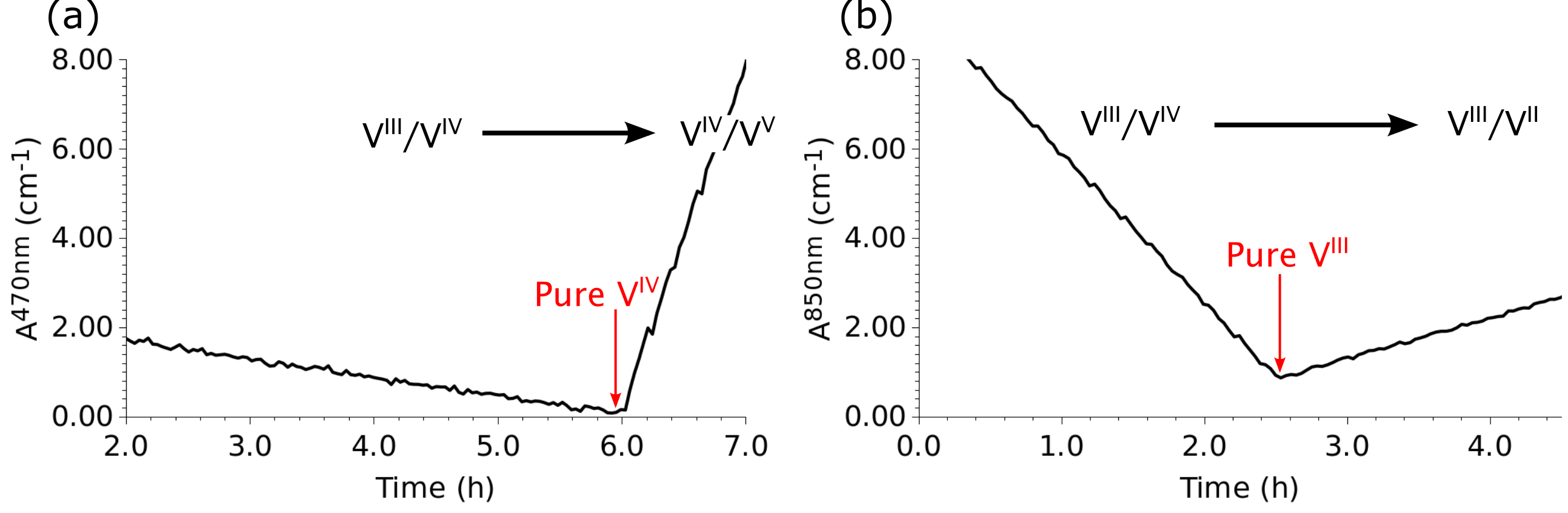
Figure S1: Plots of the absorbance $A^{\lambda}$ as a function of time at specific wavelengths during the charging process of the ${\rm V}^{\sf III}/{\rm V}^{\sf IV}$ electrolyte for (a) the positive side and (b) the negative side. A distinct inflection point can be observed in each subplot indicating the transition to a different electrolyte mixture.

S2 Empirical fitting of the positive electrolyte and calculation of $R^{2}$

This part details the fitting of the positive electrolyte absorbance using the empirical method outlined in Section 3.3.1 as well as the calculation of $R^{2}$ (also used in 3.3, Figure 6b). Figure S2a shows the absorbance of ${\rm V}^{\sf IV}/{\rm V}^{\sf V}$ at 660 nm as a function of $X_{4}$ for the four concentrations. The black dots are the experimental points ($A_{\rm exp}$) and the red line is the fitted curve ($A_{\rm p}$) obtained from Equation (22). As pointed out in the main text, the empirical fit performs as well as the analytical fit shown in Figure 6. This is further confirmed by the high value of $R^{2}$ shown in Figure S2b. The coefficient of determination is calculated at each wavelength following its classical definition

$$R^{2}=1-{SS_{\rm res}\over SS_{\rm tot}}$$

in terms of the sum of squares of residuals

$$SS_{\text{res}}=\sum_{C,X_{4}}(A_{\rm exp}-A_{\rm p})^{2}$$

where $A_{\rm p}$ denote the predicted absorbance values (plotted as red lines in Figure 6a and Figure S2a), and the total sum of squares

$$SS_{\text{tot}}=\sum_{C,X_{4}}(A_{\rm exp}-\overline{A_{\rm exp}})^{2}$$

defined as the sum over all squared differences between the observations and their overall mean.

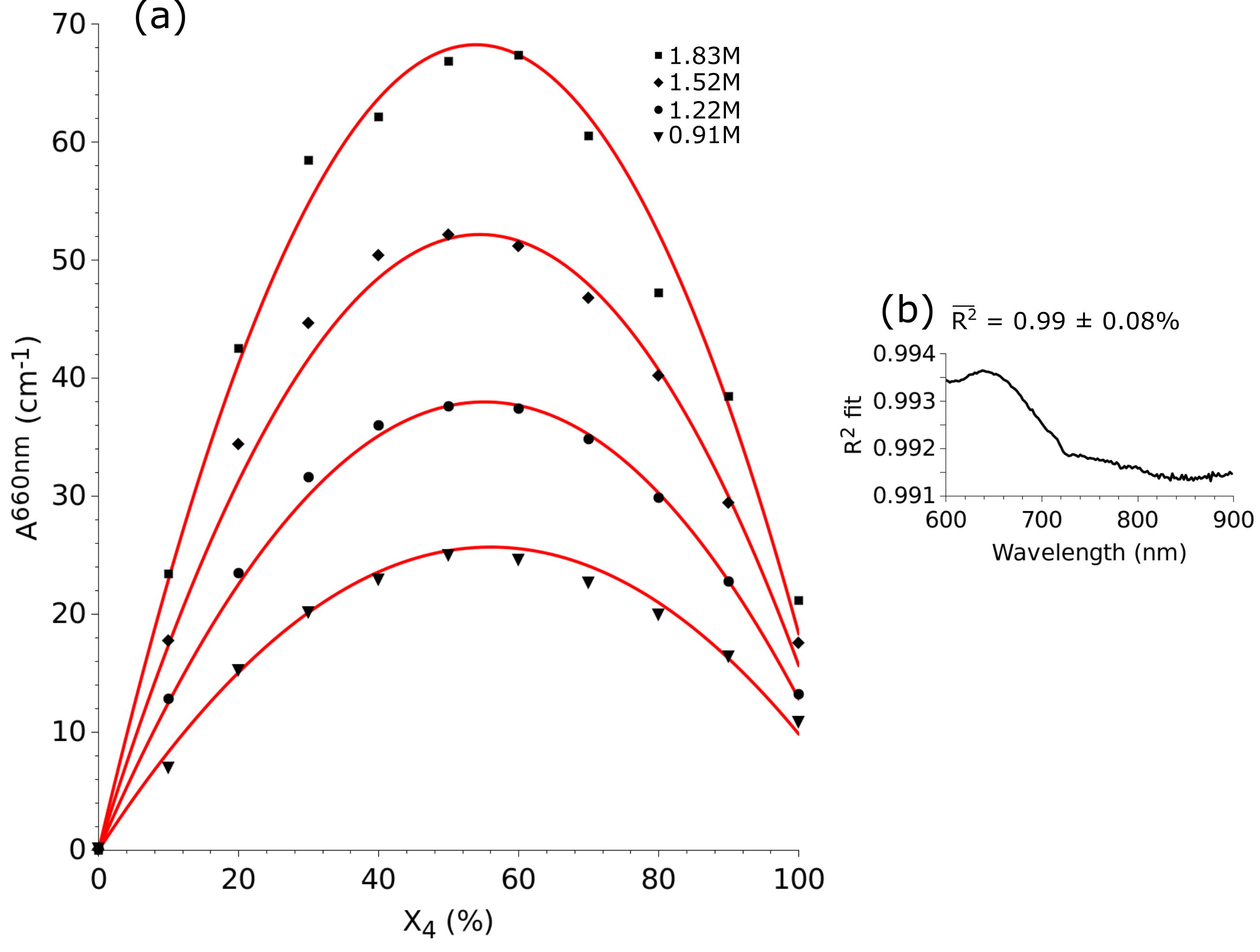
Figure S2: (a) Absorbance of the ${\rm V}^{\sf IV}/{\rm V}^{\sf V}$ mixture at 660 nm as a function of $X_{4}$ for the four total vanadium concentrations under study as measured experimentally (black dots) and fitted from the empirical Equation 22 (red curves). The right plot show the fitted (b) coefficient of determination $R^{2}$ as a function of the wavelength.

S3 Averaging of $\epsilon_{45}$

This section describes the procedure for determining the molar absorptivity of the complex, $\epsilon_{45}$, used in the spectral deconvolution of the positive electrolyte as described in Section 3.3.2 of the main text. Figure S3 shows in gray the calculated absorptivities of the complex $\epsilon_{45}$ obtained from Equation (27) for all 36 calibration samples of the positive electrolytes. In order to exclude samples where the complex is absent, those with $X_{4}=0$% or 100% were omitted. According to the model assumptions, only one unique $\epsilon_{45}$ curve should be associated with the complex, regardless of the values of $X$ or $C$. The average of the gray curves is arbitrarily chosen as a reference (depicted as the red curve) for the calibration process, yielding satisfactory deconvolution results as highlighted in the main text (with a root mean square error $E_{X}\approx 1$%). Nonetheless, the relatively high observed dispersion ($\rm\approx 3-12\%$) suggests that the absorbance model described in this study still has its limitations. Unknown non-linear effects might be at play, opening the door for potential improvements of the absorbance model in future studies.

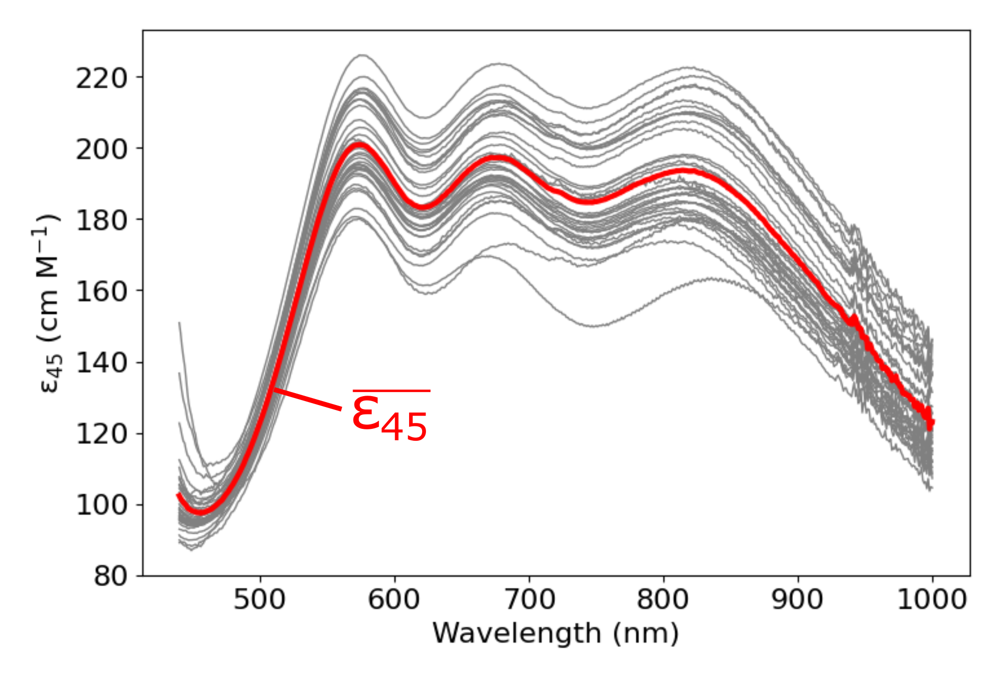
Figure S3: Molar absorptivity of the complex $\epsilon_{45}$ computed using Equation (27) for each calibration sample of the positive electrolyte (gray lines), and average absorptivity (red line) used as reference for the calibration.

S4 Parametric study for the spectral deconvolution of the positive electrolyte

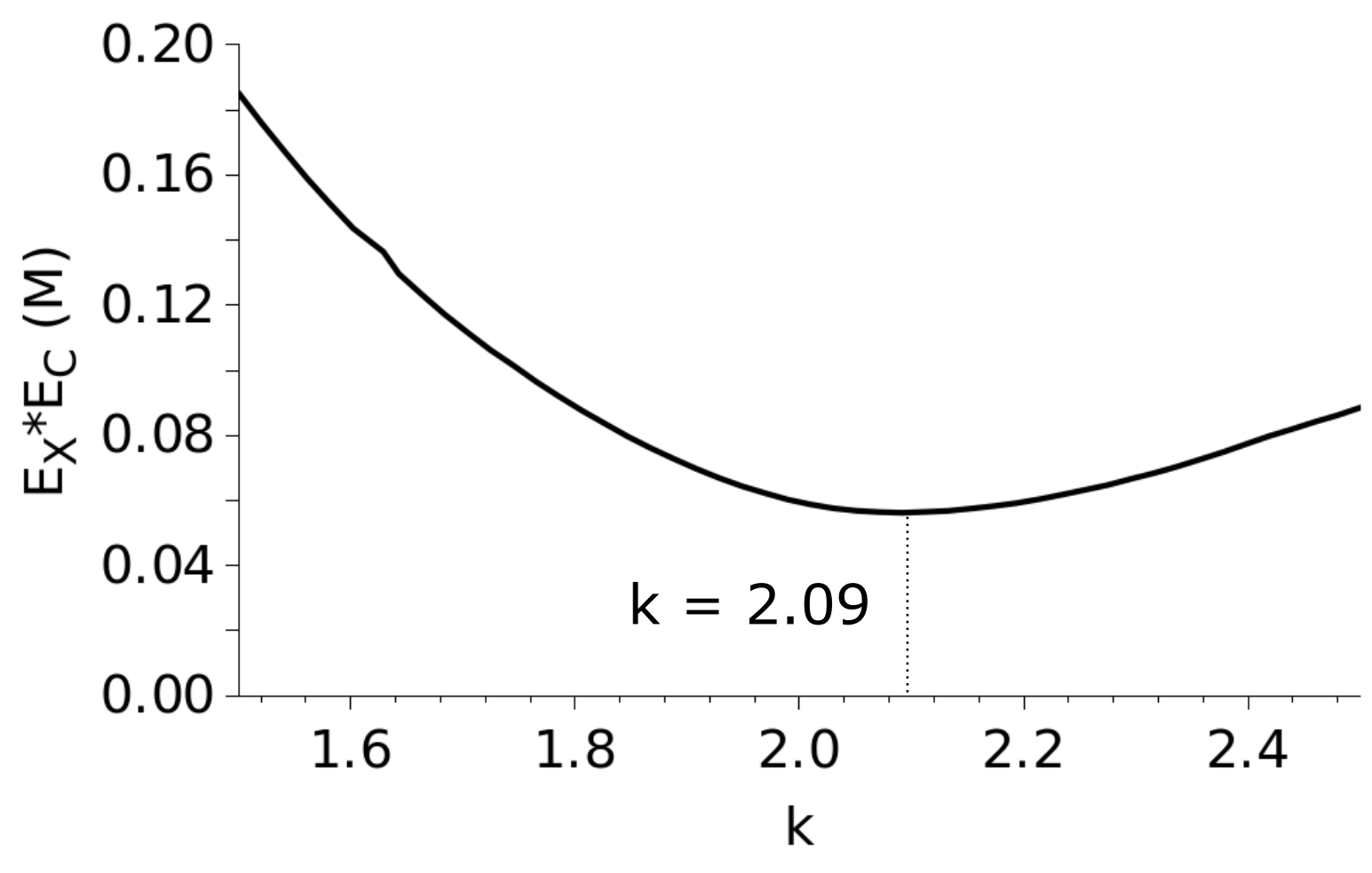
Figure S4: Product of $E_{X_{4}}$ and $E_{C}$ as a function of $k$ for the spectral deconvolution of the positive electrolyte. A clear minimum is reached for $k=2.09$.

This section presents a parametric study aimed at determining the optimal value of the power-law exponent $k$ that minimizes the overall experimental error in the spectral deconvolution of the positive electrolyte presented in Section 3.3.2 of the main text. Figure S4 illustrates the result of the study by plotting the product of the RMSE errors, $E_{X{{}_{4}}}$ and $E_{C}$, as a function of the factor $k$ involved in Equations (2), (27), and (28). Notably, the figure exhibits a clear minimum at $k=2.09$, indicating that this value represents the optimal choice for the deconvolution process. In fact, this is the value used in the results presented in Figure 8 and Table 8. It is worth noting that $2.09$ is consistent with the value $k=1.88$ indicated in Figure 1g, computed using a single wavelength of 440 nm.