onecolumn
PolyHoop: Soft particle and tissue dynamics with topological transitions
We present PolyHoop, a lightweight standalone C++ implementation of a mechanical model to simulate the dynamics of soft particles and cellular tissues in two dimensions. With only few geometrical and physical parameters, PolyHoop is capable of simulating a wide range of particulate soft matter systems: from biological cells and tissues to vesicles, bubbles, foams, emulsions, and other amorphous materials. The soft particles or cells are represented by continuously remodeling, non-convex, high-resolution polygons that can undergo growth, division, fusion, aggregation, and separation. With PolyHoop, a tissue or foam consisting of a million cells with high spatial resolution can be simulated on conventional laptop computers.
Keywords: soft particle, foam, bubble, cell, tissue, polygon
∗Correspondence: vetterro@ethz.ch
1 Introduction
A number of two-dimensional mechanical systems occurring in Nature and our daily life can be described by the dynamics of elastic, tensile hoops marking the boundaries of domains consisting of fluidic materials. The most prominent example, perhaps, is the packing of biological cells in monolayer tissues, in which cell membranes surrounding the cytoplasm can effectively be modeled as constrained adhesive polygons under tension [1, 2, 3, 4, 5, 6, 7]. Major progress in the physical understanding of epithelial dynamics has been made in recent years with 2D computer simulations [8, 9]. Foams and froths, which consist of gas bubbles enclosed by a liquid phase, are another prime example. Depending on the degree of wetness, the gas chambers in foams can exhibit a wealth of shapes and arrangements, which has made them a field of intense study at the interface of geometry and physics over decades [10, 11, 12], also computationally.
Computer simulations of such systems started mainly in the 1980s with vertex models [13, 1, 2], followed by a program named 2D-FROTH representing dry froths and foams with curved bubble boundaries [14]—a feature also particularly important in tissue biology [15, 16, 17]. These early implementations used shared polygonal boundaries between neighboring cells. More topological freedom in the form of individual, free boundaries was introduced with a C program named PLAT shortly after [18, 19]. In the 2000s and 2010s, several new two-dimensional mechanical models were developed to simulate a variety of phenomena including tissue growth and morphogenesis, cell migration and aggregation, soft particle packing, and many more. We review the history of developed computer programs that continued along the path of polygonal representations of fluidic domains in Table 1. About half of these computational models were made open-source, published under various licenses, with a tendency in the last decade toward more openness, but also more copyleft.
| Year | Name | Model description | Implementation | Performance | OS | License | Ref. |
|---|---|---|---|---|---|---|---|
| 1990 | 2D-FROTH | dry foams in mechanical equilibrium, shared polygonal boundaries | 8200 (4500) lines of Fortran 77 code, three library dependencies | demonstrated simulations with a few dozen bubbles | yes | CPC | [14] |
| 1992– 1996 | PLAT | wet foams in mechanical equilibrium, free polygonal boundaries | (5100) lines of C code, requires X/Motif libraries for GUI | demonstrated simulations with a few dozen bubbles | yes | public domain | [18, 19] |
| 2005 | — | tumor growth, free cell boundaries coupled to a Navier–Stokes solver | Fortran | demonstrated tumor tissue growth to about 900 cells | no | — | [20] |
| 2008 | — | meshed elastic cell walls immersed in a Navier–Stokes fluid | — | demonstrated growth to about 800 cells | no | — | [21] |
| 2010 | — | viscoelastic polygonal cells with cytoskeletal elements | — | demonstrated simulations with a few hundred cells | no | — | [22] |
| 2011 | — | gastrulation with elastic polygonal cell boundaries | in C using CUDA for parallelization on the GPU; reimplemented in Python using Numba [23] | demonstrated simulations with a few dozen cells | no | — | [24] |
| 2011 | VirtualLeaf | framework for plant growth with shared polygonal cell walls | () lines of C++ code, GUI based on Qt 4.6, dependencies on libiconv, libxml2, libz; no longer maintained | demonstrated simulations with a few hundred cells | yes | GPL v2 | [25] |
| 2014 | DySMaL | deformable bubble model for wet foams | Fortran program parallelized with MPI and OpenMP | 50 million timesteps with 1700 bubbles took 5 hours on 16 cores | no | — | [26] |
| 2014 | EpiCell2D | mechanical model for tissue growth with free cell boundaries | Fortran program, parallelized with MPI | dynamic simulations with a few hundred cells [27, 28] | no | — | [27] |
| 2015 | LBIBCell | polygonal cell boundaries immersed in a LBM fluid with chemical signaling | () lines of C++ code, parallelized with OpenMP, dependencies on Boost, VTK & CMake; no longer maintained | can grow a tissue to cells in a day | yes | MIT | [29] |
| 2017 | — | polygonal cell boundaries immersed in viscous Newtonian fluid | built on Chaste/cell_based [30] which depends on many third-party packages, () lines of C++ code in total | 2000 timesteps with 20 cells in a few minutes on 6 cores | yes | GPL v3 | [31] |
| 2018 | DP model | packing of elastic particles with free polygonal boundaries | — | demonstrated simulations with up to 1000 particles | no | — | [32] |
| 2016– 2022 | NCC model | cell migration, polygonal boundaries with protrusions, coupled to reaction-diffusion solver | () lines in Python using Numba [33]; reimplemented with 9600 (7600) lines in Rust [34] | single-threaded runtime of 6 hours for 49 cells simulated over 10 hours | yes | MIT or Apache | [35] |
| 2021 | LBfoam | dry and wet foams based on the LBM, similar to earlier unnamed closed-source program [36] | () lines of C++ code, including Palabos [37] | demonstrated HPC simulations with up to 300 gas cells, parallelized with MPI | yes | AGPL v3 | [38] |
| 2021 | PalaCell2D | polygonal cell boundaries immersed in a LBM fluid with chemical signaling | (8600) lines of C++ code building on Palabos, dependencies on TinyXML-2 and CMake | demonstrated simulations with up to 400 cells | no | — | [39] |
| 2021 | — | shared fluctuating polygonal cell boundaries, intercellular spaces | 2900 (2300) lines of Matlab code | demonstrated simulations with a few dozen cells | yes | public domain | [9] |
| 2021 | EdgeBased | suite of cell-based tissue models, one with polygonal cell boundaries | (6800) lines of Matlab code | tissue growth to 600 cells with 10 vertices each in 10 h | yes | GPL v3 | [40] |
| 2023 | Epimech | epithelial monolayer tissues mechanically coupled to a substrate | () lines of Matlab code, with a GUI | growth to 1600 cells in 20 hours without substrate | yes | GPL v3 | [41] |
While most of these computer programs were developed for a specific biological or physical application, quantifications of their computational performance and scalability are rare. Where it can be estimated from communicated cell counts, the used parallelization strategy or approximate runtimes, typical simulations with some dozens to a few thousand cells or bubbles require in the order of minutes to days of wallclock time. One notable exception appears to be DySMal with a large number of timesteps performed in comparably short time, although the paper did not show simulations with more than 1700 bubbles [26].
There are also a number of phase-field models to simulate the fluid dynamics of cell monolayers and foams [42, 43, 44, 45, 46, 47, 48]. The numerical burden of these grid-based approaches is large, though. Reports of the computational performance of these programs, where disclosed, range from displayed simulations of 12 cells on 36 processors [43] to simulations with 100 cells that require a month of runtime on 16 cores [47, 48]. Larger systems appear to be out of reach for these programs, possibly with the exception of the first phase-field model of biological cells [42], which was implemented in Fortran, but is not publicly available.
An additional challenge faced with most of the published programs is their level of code complexity. While the leanest implementations comprise a few thousand lines of code [14, 19, 9], the majority are found in the tens to hundreds of thousand lines [25, 29, 31, 38, 41]. This is sometimes resulting from larger frameworks they are built on or into [31, 38, 39], and can form an obstacle for their usability to other researchers, and make it harder to maintain the code.
Aside from these technical aspects, there are also methodological improvements needed to enhance the range of phenomena that can be simulated with such models. Emulsions, but also wet foams and a variety of developing biological tissues can undergo a wide range of structural changes that alter the topology at the level of bubbles or cells: they can merge or split up, aggregate or segregate, engulf or expel each other, and emerge or disintegrate. In a biological context, cells vanish from a tissue for example through apoptosis or extrusion, and they divide through mitosis. Cell fusion, on the other hand, occurs in failed cytokinesis [49], tumor progression [50], myoblasts [51], and transport vesicles [52]. With the existing computer programs, such fusion processes cannot readily be simulated.
With this paper, we introduce PolyHoop, a portable, compact and lightweight C++ program that overcomes these limitations. PolyHoop is a portmanteau of polygon and hoop, with intentional ambiguity in the meaning of “poly”, hinting at the fact that our program is designed to represent large systems consisting of many hoops or polygons. Compared to similar programs, PolyHoop offers a reduction in code volume by an order of magnitude or more, and a speedup of several orders of magnitude in cases where no explicit fluid coupling is needed, all while providing an extended feature set including the above-mentioned topological changes, in a standalone program. Comprising about 720 lines of commented code, PolyHoop is designed to be as compact and simple as possible, allowing also novices to follow the implementation, modify it, and run simulations. PolyHoop is devoid of magical numbers, error tolerances, and iterative solvers. With only 23 geometrical and physical parameters, a large variety of different dynamical systems can be simulated.
Drawing inspiration from previous models [26, 29, 32, 39], PolyHoop represents curved hoops with high spatial resolution, and allows for interstitial volume through separate representation of adjacent cell boundaries, unlike vertex models [1, 4, 5, 6, 9]. It offers the topological freedom to simulate spontaneous engulfment, splitting, fusion etc., controlled by a minimal set of parameters. System sizes in the order of a million hoops can be simulated on conventional computers, and we report the serial and parallel computational performance in easy-to-reproduce benchmarks. Combining computational performance with spontaneous topological changes, we expect PolyHoop to bridge the gap between microscopic events such as cell fusion, and macroscopic tissue structure or function, in future computational research.
2 Physical model
2.1 Continuum description
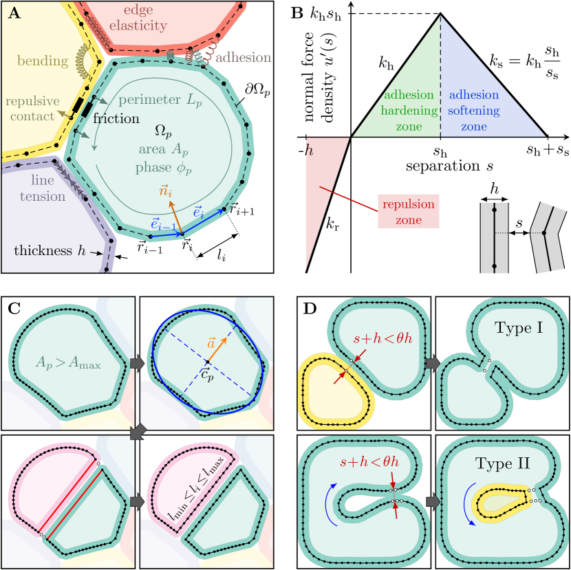
PolyHoop simulates the Newtonian dynamics of ensembles of closed hoops representing the boundaries of interacting fluidic particles (biological cells, gas bubbles, fluid droplets etc.). The interior of particle is not explicitly modeled; instead, we parameterize the position of its boundary with the vector field (Fig. 1A), and describe the ensemble by the potential energy
| (1) |
The first of the six terms in is a linearized form of elastic compression with a 2D bulk modulus of the enclosed medium of , penalizing deviations of the current particle area from a target area . The second term represents line tension with strength and hoop length . In the third summand, we account for linearly elastic tension, compression and bending of each hoop by integrating over their reference contours with length . In the integrand, is the local Cauchy strain, the local curvature, the arclength parameter running along the hoop’s contour, and the elastic dilatation and bending moduli.
To model floppy elastic particles, we couple their target areas and perimeters through the isoparametric ratio (or “asphericity” [32])
| (2) |
which equals for an unstrained circle. This coupling is unidirectional, defining the hoop length from a given area .
With the fourth energy term in Eq. 1, we model hydrostatic pressure, relevant primarily for the simulation of vertical bubbly liquids and emulsions. is the gravitational acceleration, the 2D mass density difference between the inner and outer media, and a binary flag indicating the “phase” enclosed by hoop . In a biological context where the particles represent cells, may for example be used to discriminate the cell cytosol from intra- or extracellular components, such as organelles, the extracellular matrix, etc. In simulations of a binary immiscible fluid, it discriminates between bubbles and the medium. The sign convention is such that a submerged particle containing phase is buoyant, if . is the particle’s first moment of area (defined in Eq. 14). With the fifth energy term, we allow for a complementary representation of gravity, acting on the particle boundary instead of its bulk . is the gravitational acceleration for the hoop contour, and its line mass density (mass per unit contour length). The sixth and final energy term in Eq. 1 is a double sum running over all particle pairs , accounting for bilateral interactions with an interaction potential
| (3) |
where is the spatial separation between the hoops and at their arclength positions and , and is the (virtual or physical) hoop thickness (Fig. 1A). The interaction density implemented in PolyHoop models steric repulsion and adhesion in the perhaps simplest possible way, such that a piece-wise linear traction-separation law results from it, divided into three zones (Fig. 1B). Upon volumetric overlap (negative separation ), hoop segments repel each other with repulsion strength . If the separation is positive, hoop segments attract each other with adhesion strength up to a maximum separation , beyond which the adhesion softens all the way to zero again at to ensure a continuous force transmission. Formally, this can be expressed by
| (4) |
where is the adhesion softening strength. The resulting normal force density is then given by the derivative w.r.t. the separation,
| (5) |
Note that this model allows for self-interactions (), which are relevant especially for floppy particles (large or small ). To exclude false detection of steric repulsion between nearby segments of the same hoop, we set if both and the arclength distance between the contacting points is too short, i.e., .
2.2 Discretization as polygons
We discretize the particle boundaries as polygons that automatically remodel if needed to maintain a uniform spatial resolution. Each polygon consists of a list of vertex positions , . The particle area is calculated with the shoelace formula, a special case of Green’s theorem:
| (6) |
where
| (7) |
is the 2D exterior vector product. The vertex list is cyclic, i.e., . For vertices arranged in counter-clockwise orientation, as implemented here, the absolute value bars can be dropped. From the polygon edges (Fig. 1A), the hoop length can be approximated as
| (8) |
where
| (9) |
For the elastic line integral in Eq. 1, we sum up the squared edge strains , weighted by the reference edge lengths :
| (10) |
For the bending energy, we follow the discretization proposed in [53]:
| (11) |
with nodal curvature
| (12) |
and an average reference length of the edges incident on node ,
| (13) |
To discretize the gravitational potential acting on the particle area, we require the first moment of area of each polygon, . It can be computed as [54]
| (14) |
To discretize the boundary gravitational potential, we introduce the nodal mass . As we will later dynamically adapt the polygonal discretization to keep edge lengths in a predefined range, these nodal masses do not vary greatly. Depending on the use case, and in particular with fluidic interfaces in mind, where the polygon vertices represent the interfacial shape but carry no mass, small differences in nodal inertia may be irrelevant or even undesired. We therefore harmonize the vertex masses to a constant value , and will later remove this mass scale entirely by expressing all massive parameters relative to it. With this simplification, the contour mass density is eliminated from the model and the boundary gravitational potential becomes
| (15) |
such that the effect of it on all polygon vertices is a constant uniform downward acceleration .
Finally we also discretize the interaction potential. Eq. 3 becomes a double sum over all pairs of vertices,
| (16) |
subject to the condition that the interacting vertex pair is either on different polygons (), or else, further than apart along the polygon. denotes the separation between vertex on polygon and its closest point of approach on the two edges incident on vertex on polygon . Note that this definition is asymmetric, hence the full symmetric double sum in Eq. 16. Formally, this can be expressed as
| (17) |
where
| (18) |
is the closest point on the two edges next to vertex . The barycentric edge coordinate of the closest point of approach, , allows the resulting interaction forces to be distributed to the involved vertices in proportion.
2.3 Vertex forces
From the discretized potential, the conservative nodal forces can be derived. The gradient w.r.t. the degrees of freedom of vertex of polygon reads
| (19) | ||||
Here, we used the following notation:
| (20) |
is the unnormalized inward normal vector at vertex (Fig. 1A),
| (21) |
the unit tangent vector (director) of the edge following vertex , and
| (22) |
With the ⟂ symbol we denote the perpendicular vector:
| (23) |
Notice that in Eq. 19, we assume inextensibility of the polygon edges in the bending forces for simplicity, as proposed in [53]. Moreover, to avoid the discontinuity in the coordinate of the closest point of approach between interacting hoop edges [55], we set , such that the contact forces are applied in normal direction, which considerably simplifies the interaction expression:
| (24) |
Finally, we note that the quadruple sum in the interaction term in Eq. 19 is sparse and need not actually be evaluated as such, because the interaction forces are local ( for ). Instead, spatial partitioning can be used to find non-zero contributions efficiently (see Sec. 3.4).
With the gradient of the potential defined, we can express the vertex forces. The total force vector acting on vertex is the sum of conservative and dissipative forces:
| (25) |
Here, the first force term combines all conservative forces derived from the potential, including steric repulsion and adhesion. The second term models viscous damping with a global coefficient . As a second mode of energy dissipation, we include drag (third force term), which is proportional to the squared vertex velocity, as well as to the edge length, via Eq. 20. is the dimensionless drag coefficient, and the mass density difference between the inner and outer phases as used in Eq. 1. In the fourth term, we sum over all global pairs of interacting vertices and add, for each interaction, a collision damping term in normal direction with coefficient , and a frictional force in tangential direction with dynamic Coulomb friction coefficient , proportional to the modulus of the normal interaction force
| (26) |
To arrive at this decomposition, we split the relative velocity
| (27) |
(with from Eq. 17) into a perpendicular and a parallel part:
| (28) |
Friction is only added if . Finally, using the total forces, Newton’s second law is solved for each polygon vertex:
| (29) |
3 Numerical implementation
3.1 Remodeling
PolyHoop is designed to enable arbitrarily large deformations. For applications in fluid dynamics or tissue biology, where the hoops represent fluidic interfaces, lipid bilayers, etc., dynamic remodeling of the particle/cell boundaries is essential to maintain good quality in the polygonal discretization. The polygons are automatically remodeled in each timestep to maintain an approximately uniform spatial discretization. Edges whose length exceeds a maximum value, , are bisected, introducing a new vertex in the middle. Edges whose length subceeds a minimum value, , are removed by merging their two vertices into one, positioned at the edge midpoint. Edge lengths thus remain in a predefined range, . These refining and coarsening steps intentionally break mass and momentum conservation of the particle boundaries to enable massive growth, as vertices with mass are added or removed. They do, however, conserve the masses of the enclosed particles themselves, as their target areas are unaffected.
3.2 Polygon growth, removal and division
PolyHoop can grow or shrink polygons over time by changing their target area according to
| (30) |
where is a constant area growth rate. For example for tissue simulations with biological variability, can be drawn from a random distribution for each cell individually.
Polygons whose area drops below a specified minimal value, , are removed. This feature is useful in particular for the simulation of cell extrusion from epithelial monolayers, through apoptosis, active contraction, or overcrowding.
Primarily for biological applications of proliferative tissues, polygons (cells) are divided into two when their area exceeds a threshold value, (Fig. 1C). Like the growth rate, the maximum cell area can be cell-specific and drawn from a random distribution to introduce cell-to-cell variability. Division is set to occur always through the centroid [54]
| (31) |
The long axis rule is implemented, according to which cells divide in direction of their longest extent. To find the division axis perpendicular to it (Fig. 1C, orange), we use the eigensystem of the cell’s inertia tensor, which is an intuitive way to define a cell’s orientation in space by approximating it by its own inertia ellipse (Fig. 1C, blue). For a polygon with uniform unit mass density, the inertia tensor reads [54]
| (32) |
where
| (33) |
The inertia tensor about the polygon centroid can be computed by applying the parallel axis theorem, resulting in
| (34) |
is symmetric positive semi-definite, its eigenvalues are the principal moments of inertia, and its eigenvectors are the principal axes. The shortest axis is the eigenvector with the largest eigenvalue . An efficient and robust way to find this (unnormalized) axis numerically is [56]
| (35) |
with
| (36) |
Note that for a perfectly rotationally symmetric polygon, and , resulting in . In this special case, a random division axis is drawn instead.
With the line of division defined, the polygon is cut into two at its points of intersection with the division line, and vertices are iteratively removed if necessary to prevent overlaps between the two newborn daughters (Fig. 4C, white dots). The polygons are then resealed with straight lines (strained equally to the remainder of the polygon), and the edge remodeling algorithm outlined above restores the desired spatial resolution (Fig. 4C, bottom row). The mother cell’s target area is distributed to its children in proportion to their actual area, and both children finally draw new (random) area growth rates and division areas .
3.3 Polygon fusion
Topological changes are the most computationally demanding and programmatically complex part of PolyHoop, making up more than a third of the code and accounting for about half of the total runtime in a typical simulation when enabled. Aside from division and removal described above, two further types of topological changes (I and II) are implemented, which increment or decrement the number of polygons in the system, subsumed under “polygon fusion” here (Fig. 1D). Type I refers to the merger of two touching distinct polygons into one, which decrements the polygon count. Type II refers to “self-fusion”, i.e., the splitting of a polygon into two due to two distant segments of the same polygon touching, which increments the polygon count. Both fusion types can occur in two variants each: For Type I, the two touching polygons may either be external to each other (as shown in Fig. 1D, top row) or one inside the other. Conversely, for Type II, the newly spawned polygon may either be outside the existing one or inside (as shown in Fig. 1D, bottom row). When polygons internalize or externalize in this process, they are reoriented into anti-clockwise vertex order, as PolyHoop requires all polygons to be anti-clockwise for simplicity. Whether a polygon is enclosing the other is tested with an efficient ray casting algorithm [57] during the fusion event.
Fusion events are triggered based on the local degree of mutual interpenetration of pairs of polygon segments, which is equivalent to contact stress criteria that depend on the mutual contact depth, such as in Hertzian models. We opted for a minimal, generic model with a single, intuitive and easy-to-control parameter, the fusion threshold . If , the fusion feature is disabled. If , polygons fuse immediately when they come in physical contact. In general, a value in between lets polygons fuse when they press against one another sufficiently to let , with a negative separation between polygon segments (Fig. 1B). When this overlap criterion is met, the polygons are broken up and their vertices are iteratively removed in the vicinity of the closest point of contact, until they lie sufficiently (i.e., a minimal distance of ) apart such that the two gaps can be rejoined without residual overlaps (Fig. 1D).
3.4 Contact detection
Hoop interactions, if enabled, can make up a large fraction of the overall computational cost, because generally, any pair of vertices can be in contact. To reduce the quadruple sum in Eq. 19 to effectively a double sum running over all polygons and their vertices, we employ spatial partitioning [58] using linked lists. Within the global bounding box of all polygons, the simulation space is divided into square boxes with side length , which ensures that interacting vertex pairs are no more than one box apart. Instead of the current largest edge length , the upper bound could also be used for simplicity, but we observed generally better performance with the former. A global array then stores a pointer to the first vertex in each box, and each vertex holds a pointer to the next vertex in the same box. Checking for polygon interactions then reduces to a loop over all vertices and a loop over all vertices contained in the local group of boxes around . This procedure reduces the time complexity of contact detection from squared to linear in the number of vertices. The boxes are recomputed in each timestep for simplicity.
3.5 Time integration
For the discontinuous evolution of a particle system with instantaneous topological changes as implemented in PolyHoop, multi-step or implicit time integration methods are difficult to formulate. We therefore propagate the vertex positions and velocities with the semi-implicit Euler method:
| (37) | ||||
where is the timestep size. Since we eliminated all masses from the program code (), the vertex forces are effectively accelerations.
| Symbol | Default value | Constraints | Dimension | Description |
| Geometric parameters | ||||
| 0.01 | L | Edge thickness | ||
| L | Minimum edge length | |||
| L | Maximum edge length | |||
| — | Target isoparametric ratio | |||
| 1 | — | L2/T | Area growth rate | |
| L2 | Minimum polygon area (for cell removal) | |||
| L2 | Maximum polygon area (for cell division) | |||
| L | Adhesion hardening zone size | |||
| L | Adhesion softening zone size | |||
| — | Fusion threshold | |||
| Material parameters | ||||
| M/L2T2 | Area stiffness | |||
| — | ML/T2 | Boundary line tension | ||
| ML/T2 | Tensile rigidity | |||
| 0 | ML3/T2 | Bending rigidity | ||
| 1/MT2 | Repulsion stiffness | |||
| 1/MT2 | Adhesion stiffness | |||
| 0 | — | Dynamic Coulomb friction coefficient | ||
| 0 | — | M/L2 | Fluid mass density | |
| Other parameters | ||||
| 0 | — | L/T2 | Gravitational acceleration | |
| 0 | — | L/T2 | Edge gravitational acceleration | |
| M/T | Viscous damping coefficient | |||
| 1/T | Contact damping coefficient | |||
| 0 | — | Drag coefficient | ||
| T | Time increment | |||
| 1 | fixed | M | Vertex mass (not in the code) | |
4 Applications
PolyHoop can be applied to a broad range of 2D elastic or free surface problems governed by effectively 23 physical parameters—ten geometrical, eight material, and five others (not counting the numerical time increment). Table 2 lists them all, including constraints that need to be respected, and a set of simple default values that quickly produce usable simulation output and may serve as a starting point to find working parameters for specific applications. We now showcase a selection of scenarios that can be represented with these 23 model parameters.
4.1 Biological tissues
We start with a series of biological examples. The classical application is a growing epithelial monolayer tissue. Fig. 2A and Movie 1 show a simulation with about 1000 cells with thin membranes () whose equilibrium shape is a circle (). The cells are adhesive, mildly compressible, and their membranes are governed by cortical tension and relatively weak line elasticity (Table 3). Bending, fusion, friction, gravity, and drag are disabled by setting their respective coefficients to zero. The simulation starts with a single cell with unit radius. Cells divide upon reaching an area of , and grow at a rate drawn from a normal distribution for each cell independently. For demonstration purposes, negative growth rates are allowed here, and cells undergo apoptosis (i.e., they are removed) when they become small. As shown in the closeup in Fig. 2A, the cells end up being non-convex, with curved membranes. Simulations like these are widespread in computational biology and in essence reproducible with existing software [20, 21, 22, 25, 27, 29, 31, 39, 40, 41]; with PolyHoop, they now run in a few minutes.
PolyHoop is also suited to study active motion (motility), migration, collective behavior, or aggregation/segregation. Although this is not implemented in the supplied default code, a localized attractor, for example, can be added with a single line of additional code, to model chemotaxis, durotaxis, or similar phenomena. In Fig. 2B and Movie 2, we picked 20 cells at random (red) and let them migrate toward a single point with a radial attractive potential. With such simulations, open 2D problems in cell motility [59] may be addressable efficiently.
Also non-confluent, structured tissues can be represented. Fig. 2C shows an example simulation with epithelial vesicles (brown cells) arranged in monolayer rings surrounding a luminar region (light blue). The parametric setup is similar to the previous examples (Table 3), with the notable exception that we set the isoparametric ratio to that of squares, , such that in absence of bending and cortical tension, the cells are mechanically satisfied with a rectangular shape.
| Fig. | ||||||||||||||||||||||||
|---|---|---|---|---|---|---|---|---|---|---|---|---|---|---|---|---|---|---|---|---|---|---|---|---|
| 2A | var† | |||||||||||||||||||||||
| 2B | ||||||||||||||||||||||||
| 2C | — | |||||||||||||||||||||||
| 2D | — | |||||||||||||||||||||||
| 2E | ||||||||||||||||||||||||
| 2F | — | |||||||||||||||||||||||
| 2G | — | |||||||||||||||||||||||
| 2H | ||||||||||||||||||||||||
| 3 | var‡ | |||||||||||||||||||||||
| 4A,B | ||||||||||||||||||||||||
| 4C,D | ||||||||||||||||||||||||
| †Randomly drawn from a normal distribution with a mean and standard deviation of (including negative values). | ||||||||||||||||||||||||
| ‡Randomly drawn from a lognormal distribution with mean and coefficient of variation . | ||||||||||||||||||||||||
4.2 Amorphous materials
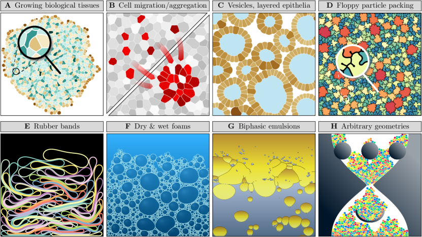
A further field of application is the study of amorphous materials and their dense packing, jamming, rheology, etc., in the spirit of recent numerical work [32, 17, 60]. To illustrate an extreme case, we close-packed an ensemble of polydisperse floppy particles with excess circumference () (Fig. 2D). For this simulation, the particles were set to be mildly compressible, weakly adhesive, with a slightly thicker boundary () driven by line elasticity and weak bending rigidity (Table 3). Line tension, gravity, friction etc. were disabled. The resulting configuration exhibits interlocked particles with tight local folds to accommodate the long boundaries. Although their genesis may be different (i.e., without internal joints), these particle shapes resemble those of the the puzzle-shaped epidermal cells of Arabidopsis thaliana leaves [61].
4.3 Elastic bands
To showcase an application dominated by bending and gravitational forces, we simulated the downfall and packing of 100 thick elastic bands. Boundary gravity () compresses the initially vertically piled-up circular rings to the point where they partially align into parallel bundles (Fig. 2E). For an animated version, see Movie 3. For this simulation, we set the area stiffness, line tension, and adhesion parameter values to zero, but increased the thickness and bending rigidity (Table 3). PolyHoop thus enables simulations of the packing of elastic rods (previously performed on linear rods [62, 55]) with circular hoops.
4.4 Foams and emulsions
Also belonging to the class or amorphous solids, but worth mentioning separately here for their historical significance (cf. Table 1), are foams and emulsions. A relatively wet foam is shown in Fig. 2F, produced by letting a polydisperse collection of nearly incompressible bubbles, initially circular in shape and randomly placed in the plane, drop under the action of gravity. Governed by surface tension and weak cohesion (Table 3), the bubbles deform and coalesce into a foamy structure with a free upper surface (Movie 4).
Perhaps technically the most challenging application in this exhibition is the simulation of a binary emulsion in which oil drops in an aqueous medium freely fuse and split (Fig. 2G). In this simulation, we use a mass density difference of between the two phases to let the oil drops float upward in response to hydrostatic pressure, slowed down by drag () (Table 3). With a fusion threshold of , oil drops pressing against each other merge, broken bubble boundaries retract driven by interfacial tension, and a free water-oil interface forms naturally, separating the two phases (Movie 5). Note that PolyHoop poses no limit to the recursion depth in the drop-in-drop cascade. For demonstration purposes, we placed water droplets in the oil drops here, which are then joined by further droplets that spontaneously form from the interfaces breaking up when drops fuse. The entire simulation completes in about 10 minutes. Simulations of this kind may for instance be used to advance earlier 2D foaming studies [36, 38] to a regime involving larger topological rearrangements.
4.5 Complex geometries
PolyHoop offers native support for arbitrarily shaped geometrical domains and obstacles. We demonstrate this with a simulation of about 1000 soft sticky particles dropping in an hourglass-like geometry with four additional curved objects in the way (Fig. 2H, Movie 6). For this simulation, we also turned on friction (, Table 3). Rigid objects, which can serve both as confining bounds and obstacles, are implemented in PolyHoop with a simple, flexible approach requiring minimal coding: They are treated as normal particles, with two exceptions: They are not coarsened to maintain a preset resolution of curved regions (but refined to ensure , enabling efficient local contact detection), and their vertex positions are not updated to make them immobile. This delegates the geometric definition of rigid domain boundaries to the input file (see Sec. 6), and renders specialized collision handling with primitive shapes unnecessary.
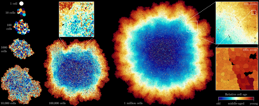
4.6 Large-scale simulation
Finally, we return to a biophysical application to demonstrate the scale PolyHoop can reach. A strongly proliferative, cancer-like tissue is grown from a single cell to a million cells (Fig. 3). To our knowledge, this is the first published report of a comparable simulation exceeding cells with high boundary resolution. Cell boundaries have a mean resolution of vertices, totaling in about 72 million simulated vertices in the final tissue. To avoid excessive pressure buildup in the interior of the tissue due to the fast growth speed, cells are grown only if in this simulation. At around cells (Fig. 3, bottom left), we observe a transition from spatially uniform cell proliferation to a radial gradient in the relative cell age, with a central region where the compressed cells (blue) are able to grow to their division area only sporadically, and a rugged rim consisting mainly of very young, proliferative cells (red). Closeups reveal regions exhibiting sharp cell age boundaries within the tissue. This example demonstrates how organ-scale emergent features can be studied with PolyHoop without relinquishing cellular fidelity. See Movie 7 for an animated version.
5 Parallelization and computational efficiency
Up to caching effects, the total serial time complexity for simulations with PolyHoop is , where is the number of polygons, is the mean number of vertices per polygon, and is the simulated time duration in units of steps. The number of output frames, , and the number of time steps per frame, , are simulation output parameters that can be set in the code. The runtime of the program thus scales linearly with the total number of vertices, . Higher spatial resolution, temporal resolution, or number of simulated polygons affect the runtime proportionally.
PolyHoop is parallelized for shared-memory computers, using OpenMP. With just six omp parallel for directives, the main loops for bounding box computation, force computation, polygon interactions, fusion testing, remodeling, and time propagation are parallelized without explicit use of threading expressions, leaving the serial flow of the source code untouched. Three relevant code segments are not parallelized: I/O, the construction of neighbor lists (because of speedup limitations [63]), and the execution of topological changes. The latter is due to changes in polygon count and the involvement of polygons in multiple topological changes in a single timestep, which makes it challenging to apply simple parallelization strategies.
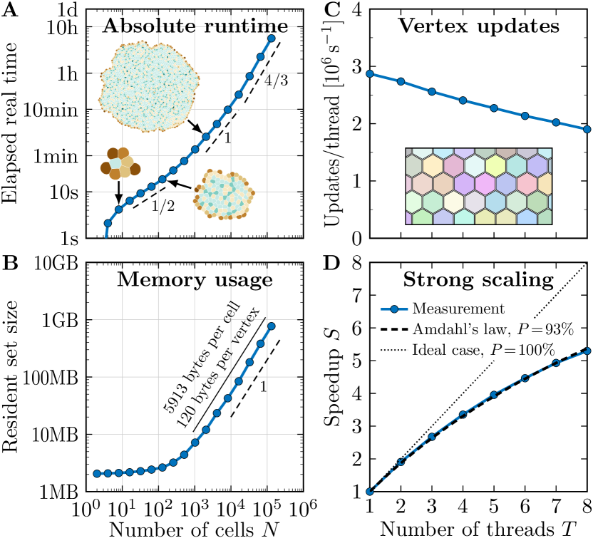
To assess the computational efficiency in absolute terms, we measured the wallclock time in a typical biological tissue simulation with exponential growth on an ordinary modern laptop computer using 8 threads. Starting from a single proliferative cell, a tissue was produced by successive cell growth and division, similar to Figs. 2A and 3, and the elapsed time was recorded for each doubling of the cell count (Fig. 4A). For a few hundred cells, we observe square-root time complexity in the number of grown cells , presumably due to cache locality. In an intermediate range with some thousand cells, the runtime increases linearly with the number of cells, until about , which is reached in about 12 minutes at a resolution of vertices per cell. Beyond that, the runtime is superlinear with power-law exponent due to a slow-down of proliferation caused by pressure building up in the interior of the tissue, which can in principle be avoided with lower growth rates. A time complexity of is also observed in similar simulations in 3D [64]. A tissue consisting of cells is grown in less than six hours. For this performance benchmark, we excluded I/O and cell fusion testing.
In an analogous simulation, we measured the memory usage under Red Hat Enterprise 7.9 and found the expected asymptotically linear scaling (Fig. 4B). The total memory complexity is thus . Each vertex uses 72 bytes of memory in IEEE double precision on a 64bit architecture: 7 floating-point numbers for the vertex position, velocity, acceleration, and target length of the adjacent edge, and 2 indices or pointers for the polygon affiliation and forward vertex linkage in the space partitioning grid. Including per-polygon data of 64 bytes each, the spatial grid, temporaries, and bookkeeping overhead, we measured an overall memory requirement of about 120 bytes per vertex in a typical tissue growth scenario. A simulation with polygons, consisting of vertices each, therefore requires approximately 60 MB of main memory in total. A large high-fidelity simulation with polygons, consisting of vertices each, will consume about 12 GB, and will thus still easily fit into the main memory of most ordinary modern computers.
PolyHoop scales well on multi-core CPUs. The number of vertex updates that are performed per second and per thread in a large hexagonal close-packing setting (Fig. 4C, inset), in which all interior edges are in active contact with neighboring polygons, drops by only a third from almost 3 million in serial mode to about 2 million with 8 threads (Fig. 4C). We observe the strong-scaling behavior to follow Amdahl’s law very closely, with a speedup of , where is the parallel portion and the number of threads (Fig. 4D). The remaining 7% are largely due to the serial placement of vertices into the spatial partitioning grid.
6 Usage instructions
PolyHoop was developed to be highly portable, but it requires a compiler compatible with the C++11 standard. For multithreading support, the OpenMP 3.1 specification or newer is additionally required. We tested it using GCC v4.8.2–12.2.0, Clang/LLVM v3.6.0–15.0.7, and ICC v14.0.1–19.1.0. Compiling PolyHoop is as simple as running
g++ -fopenmp -O3 -o polyhoop polyhoop.cpp
or an equivalent command. PolyHoop can be compiled for serial execution by omitting the OpenMP compile option.
To run a simulation, set the desired parameters in polyhoop.cpp (lines 13–42), compile it, and execute the binary by typing
OMP_NUM_THREADS=8 ./polyhoop
or similar. If PolyHoop is compiled with OpenMP support and the number of threads is not specified, the selection of a suitable number of threads is delegated to OpenMP.
PolyHoop reads in a mandatory input file named ensemble.off from the current working directory, specifying the initial configuration in GeomView’s Object File Format (OFF) [65]. Since OFF specifies vertex coordinates in three dimensions ,,, but PolyHoop uses only two ( and ), the coordinate is used to indicate the phase of the polygon containing the vertex. is expected to be an integer that, if odd, denotes phase , and if even, . The input file only specifies vertex positions; velocities are initialized to zero. The first polygons in the input file are treated as rigid obstacles (see Sec. 4.5). can be set in the source file.
The creation of such input files representing suitable initial starting conditions for different applications is left to the user. The supplied default input file ensemble.off contains a single 40-node circular hoop with unit radius, as used in the tissue growth simulations showcased in Figs. 2A, 3 and 4A,B. The default parameter setup (Table 2) grows a 128-cell tissue out of this single initial cell in about 20 seconds on an Intel Core i9-9880H CPU using four threads.
PolyHoop writes the simulated configurations at specified time intervals (every timesteps) to the current working directory, naming them frame%06d.vtp. With each output frame, a single-line status report is printed to the command line. The output files are in the VTK ASCII polygon format [66]. For each polygon in the ensemble, they store the area, perimeter and coordination number (the number of other polygons each polygon is separated from by a distance shorter than ). The simulation output can be visualized and animated by opening the VTK file series in ParaView (https://paraview.org). For non-convex polygons, the Extract Surface and Triangulate filters need to be applied to ensure correct visual representation. Similar to the input file, the phase of each polygon is stored in the unused coordinate of the output VTK files, as a binary flag .
7 Discussion and outlook
PolyHoop is an exceptionally lightweight standalone program that enables the simulation of a wide variety of dynamic phenomena governed by constrained visco-elastic hoops in 2D, such as monolayer tissues, emulsions, or other ensembles of soft deformable particles. PolyHoop stands out of the crowd of related model implementations [29, 32, 39] in mainly three aspects:
-
•
Topological flexibility. Hoops/polygons can be broken up and rejoined, tissues can grow together or detach, new cells can emerge through cell division or disappear by death or extrusion, bubbles can merge or split up.
-
•
Computational performance. PolyHoop is designed to be particularly lean and efficient, making it the first of its kind (to our knowledge) to enable large-scale simulations with hundreds of thousands or even millions of polygons with high spatial resolution. Biological tissue simulations of the size of entire organs can be simulated on customary computers, without requiring access to the brute force of cluster computing infrastructure or GPUs.
-
•
Accessibility. PolyHoop is completely free and open-source. Comprising only just above 700 lines of compact, simple, commented C++ code, it is easy to handle, extend and embed in other programs. Importantly, it has no dependencies, making it exceptionally independent and portable. Thanks to the 3-clause BSD license under which PolyHoop is published, both commercial and non-commercial uses are permitted.
With PolyHoop, computer simulations of 2D tissue morpogenesis enter a regime in which open questions at macroscopic length scales can be addressed numerically with high spatial resolution of individual cells. Complex intertwined cell shapes have recently been discovered in pseudostratified epithelia [67, 68], and their role in organogenesis and patterning is a subject of ongoing research [69]. Interkinetic nuclear migration, a process in which migrating nuclei can strongly deform the cells, remains largely mysterious [70]. Studying these phenomena in silico requires models that offer a degree of geometrical flexibility that allows to link cell shape to tissue function and morphology. PolyHoop is a high-throughput tool that enables such simulations not only with some dozens of cells, but with hundreds of thousands.
A particular strength of PolyHoop, which also happens to be a core application it was developed for, is the growth of proliferative tissue to developmentally or medically relevant sizes, and other morphogenetic events on that scale. The cell count of the Drosophila wing disc ( [71]), for example, one of the most-studied organs in developmental biology, is reached in about 1.5 hours on a typical modern 8-core CPU, with each cell discretized by 50 vertices, starting from a single cell (Fig. 4A). Another natural application is macroscopic growth of malignant tumors (Fig. 3), which are linked to aberrant cell shape and impairment of structural tissue integrity [72].
With polygon fusion, PolyHoop adds a feature to the pool of 2D free-boundary evolvers that enables the simulation of topological transitions occurring in a variety of bubbly systems, from emulsions to biological tissues. Cell fusion is crucial in tissue development [73], but not commonly included in cell-based simulations of tissue development. Our program is well suited to simulate such processes. The current implementation uses a simple geometrical indentation criterion with parameter to trigger fusion, which is equivalent to a compressive stress threshold. With minimal changes to the source code, cells could be made to fuse based on other conditions such as time, position, cell size and shape, cell type, and potentially biochemical signals.
Several further extensions and generalizations of the present model are easy to recognize. For simplicity, all polygons in PolyHoop share the same constitutive relationships and material parameters (apart from the area growth rate and division area threshold, which are drawn from random distributions in the supplied code). It is straightforward to make these properties members of the individual polygons, or even vertices or edges if needed, with only a few lines of code to be changed. This will allow to simulate different types of particles in the ensemble, or non-uniform or inhomogeneous material behavior such as differential cell adhesion and cell polarity. Other conceivable extensions include active or Brownian motion, tension fluctuations [9, 74], and the coupling to fluid dynamics or reaction-diffusion solvers, as offered by other frameworks for applications in biology [29, 39], among others. For the simulation of realistic emulsions with deeply nested phases, it may also be desirable to make the hydrostatic pressure dependent on the vertical immersion depth in the surrounding phase rather than on the global position, as currently implemented. For applications in which the hoops represent actual physical entities (such as elastic threads or cell membranes) rather than just marking the boundaries between immiscible fluid phases, it could be useful to extend PolyHoop to allow for the rupture of hoops without immediate resealing. That is to say, allowing the polygons to have holes; to be open lines with endpoints rather than closed hoops.
On the numerical side, certain room may exists for further performance improvements. The computational performance of the present implementation is largely memory access-limited, implying that it could potentially benefit from parallelization for distributed memory systems, for instance with MPI. Moreover, a more elaborate bookkeeping of nearby vertex pairs, for example with Verlet lists [75], could speed up simulations further, considering that about 60–90% of the runtime is spent in contact detection in typical tissue growth scenarios. For PolyHoop, we have deliberately resorted to a simple and compact solution using repeatedly computed linked cell lists and parallelization with OpenMP precompiler directives.
Finally, we wish to make the interested reader aware of model developments that strive to offer functionality similar to that of PolyHoop in 3D [76, 77, 78, 79, 80, 64, 81], albeit mostly without some of the topological transitions implemented here, and naturally at substantially greater computational cost and geometrical complexity.
Acknowledgement
We thank Marius Almanstötter for help with parameter testing, as well as Marco Meer and the group of Bastien Chopard for valuable discussions. Financial support from the Swiss National Science Foundation by Sinergia grant no. 170930 is gratefully acknowledged.
Competing Interests
The authors declare that they have no competing interests.
References
- Kawasaki et al. [1989] K. Kawasaki, T. Nagai, and K. Nakashima. Vertex models for two-dimensional grain growth. Phil. Mag. B, 60:399–421, 1989. 10.1080/13642818908205916.
- Weliky and Oster [1990] M. Weliky and G. Oster. The mechanical basis of cell rearrangement I. Epithelial morphogenesis during Fundulus epiboly. Development, 109:373–386, 1990. 10.1242/dev.109.2.373.
- Graner and Sawada [1993] F. Graner and Y. Sawada. Can Surface Adhesion Drive Cell Rearrangement? Part II: A Geometrical Model. J. Theor. Biol., 164:477–506, 1993. 10.1006/jtbi.1993.1168.
- Nagai and Honda [2001] T. Nagai and H. Honda. A dynamic cell model for the formation of epithelial tissues. Philos. Mag. B, 81:699–719, 2001. 10.1080/13642810108205772.
- Farhadifar et al. [2007] R. Farhadifar, J.-C. Röper, B. Aigouy, S. Eaton, and F. Jülicher. The Influence of Cell Mechanics, Cell-Cell Interactions, and Proliferation on Epithelial Packing. Curr. Biol., 17:2095–2104, 2007. 10.1016/j.cub.2007.11.049.
- Hufnagel et al. [2007] L. Hufnagel, A. A. Teleman, H. Rouault, S. M. Cohen, and B. I. Shraiman. On the mechanism of wing size determination in fly development. Proc. Natl. Acad. Sci. U.S.A., 104:3835–3840, 2007. 10.1073/pnas.0607134104.
- Vetter et al. [2019] R. Vetter, M. Kokic, H. F. Gómez, L. Hodel, B. Gjeta, A. Iannini, G. Villa-Fombuena, F. Casares, and D. Iber. Aboav-weaire’s law in epithelia results from an angle constraint in contiguous polygonal lattices. BioRxiv, 2019. 10.1101/591461.
- Bi et al. [2015] D. Bi, J. H. Lopez, J. M. Schwarz, and M. L. Manning. A density-independent rigidity transition in biological tissues. Nat. Phys., 11:1074–1079, 2015. 10.1038/nphys3471.
- Kim et al. [2021] S. Kim, M. Pochitaloff, G. Stooke-Vaughan, and O. Campàs. Embryonic Tissues as Active Foams. Nat. Phys., 2021. 10.1038/s41567-021-01215-1.
- Weaire [1992] D. Weaire. Some lessons from soap froth for the physics of soft condensed matter. Phys. Scr., 1992:29–33, 1992. 10.1088/0031-8949/1992/T45/006.
- Weaire et al. [2007] D. Weaire, V. Langlois, M. Saadatfar, and S. Hutzler. Foam as granular matter, volume 8 of Lecture Notes in Complex Systems, chapter 1, pages 1–26. World Scientific, 2007. 10.1142/9789812771995_0001.
- Weaire and Hutzler [2009] D. Weaire and S. Hutzler. Foam as a complex system. J. Phys.: Condens. Matter, 21:474227, 2009. 10.1088/0953-8984/21/47/474227.
- Odell et al. [1981] G.M. Odell, G. Oster, P. Alberch, and B. Burnside. The mechanical basis of morphogenesis: I. Epithelial folding and invagination. Dev. Biol., 85:446–462, 1981. 10.1016/0012-1606(81)90276-1.
- Kermode and Weaire [1990] J. P. Kermode and D. Weaire. 2D-FROTH: a program for the investigation of 2-dimensional froths. Comput. Phys. Commun., 60:75–109, 1990. 10.1016/0010-4655(90)90080-K.
- Ishimoto and Morishita [2014] Y. Ishimoto and Y. Morishita. Bubbly vertex dynamics: A dynamical and geometrical model for epithelial tissues with curved cell shapes. Phys. Rev. E, 90:052711, 2014. 10.1103/PhysRevE.90.052711.
- Perrone et al. [2016] M. C. Perrone, J. H. Veldhuis, and G. W. Brodland. Non-straight cell edges are important to invasion and engulfment as demonstrated by cell mechanics model. Biomech. Model. Mechanobiol., 15:405–418, 2016. 10.1007/s10237-015-0697-6.
- Boromand et al. [2019] A. Boromand, A. Signoriello, J. Lowensohn, C. S. Orellana, E. R. Weeks, F. Ye, M. D. Shattuck, and C. S. O’Hern. The role of deformability in determining the structural and mechanical properties of bubbles and emulsions. Soft Matter, 15:5854–5865, 2019. 10.1039/C9SM00775J.
- Bolton and Weaire [1992] F. Bolton and D. Weaire. The effects of Plateau borders in the two-dimensional soap froth. II. General simulation and analysis of rigidity loss transition. Phil. Mag. B, 65:473–487, 1992. 10.1080/13642819208207644.
- Bolton and Dunne [1996] F. Bolton and F. F. Dunne. Software PLAT: A computer code for simulating two-dimensional liquid foams, 1996. https://github.com/fbolton/plat.
- Rejniak [2005] K. A. Rejniak. A Single-Cell Approach in Modeling the Dynamics of Tumor Microregions. Math. Biosci. Eng., 2:643–655, 2005. 10.3934/mbe.2005.2.643.
- R. et al. [2008] Dillon R., Owen M., and Painter K. A single-cell based model of multicellular growth using the immersed boundary method, pages 1–16. Contemporary Mathematics. American Mathematical Society, 2008. ISBN 9780821842676.
- Jamali et al. [2010] Y. Jamali, M. Azimi, and M. R. K. Mofrad. A Sub-Cellular Viscoelastic Model for Cell Population Mechanics. PLOS ONE, 5:1–20, 2010. 10.1371/journal.pone.0012097.
- van der Sande et al. [2020] Maarten van der Sande, Yulia Kraus, Evelyn Houliston, and Jaap Kaandorp. A cell-based boundary model of gastrulation by unipolar ingression in the hydrozoan cnidarian Clytia hemisphaerica. Dev. Biol., 460:176–186, 2020. 10.1016/j.ydbio.2019.12.012.
- Tamulonis et al. [2011] C. Tamulonis, M. Postma, H. Q. Marlow, C. R. Magie, J. de Jong, and J. Kaandorp. A cell-based model of Nematostella vectensis gastrulation including bottle cell formation, invagination and zippering. Dev. Biol., 351:217–228, 2011. 10.1016/j.ydbio.2010.10.017.
- Merks et al. [2011] R. M. H. Merks, M. Guravage, D. Inzé, and G. T. S. Beemster. VirtualLeaf: An Open-Source Framework for Cell-Based Modeling of Plant Tissue Growth and Development. Plant Physiol., 155:656–666, 2011. 10.1104/pp.110.167619.
- Kähärä et al. [2014] T. Kähärä, T. Tallinen, and J. Timonen. Numerical model for the shear rheology of two-dimensional wet foams with deformable bubbles. Phys. Rev. E, 90:032307, 2014. 10.1103/PhysRevE.90.032307.
- Mkrtchyan et al. [2014] A. Mkrtchyan, J. Åström, and M. Karttunen. A new model for cell division and migration with spontaneous topology changes. Soft Matter, 10:4332–4339, 2014. 10.1039/C4SM00489B.
- Madhikar et al. [2021] P. Madhikar, J. Åström, B. Baumeier, and M. Karttunen. Jamming and force distribution in growing epithelial tissue. Phys. Rev. Res., 3:023129, 2021. 10.1103/PhysRevResearch.3.023129.
- Tanaka et al. [2015] S. Tanaka, D. Sichau, and D. Iber. LBIBCell: a cell-based simulation environment for morphogenetic problems. Bioinformatics, 31:2340–2347, 2015. 10.1093/bioinformatics/btv147.
- Pitt-Francis et al. [2009] J. Pitt-Francis, P. Pathmanathan, M. O. Bernabeu, R. Bordas, J. Cooper, A. G. Fletcher, G. R. Mirams, P. Murray, J. M. Osborne, A. Walter, S. J. Chapman, A. Garny, I. M. M. van Leeuwen, P. K. Maini, B. Rodríguez, S. L. Waters, J. P. Whiteley, H. M. Byrne, and D. J. Gavaghan. Chaste: A test-driven approach to software development for biological modelling. Comput. Phys. Commun., 180:2452–2471, 2009. 10.1016/j.cpc.2009.07.019.
- Cooper et al. [2017] F. R. Cooper, R. E. Baker, and A. G. Fletcher. Numerical Analysis of the Immersed Boundary Method for Cell-Based Simulation. SIAM J. Sci. Comput., 39:B943–B967, 2017. 10.1137/16M1092246.
- Boromand et al. [2018] A. Boromand, A. Signoriello, F. Ye, C. S. O’Hern, and M. D. Shattuck. Jamming of Deformable Polygons. Phys. Rev. Lett., 121:248003, 2018. 10.1103/PhysRevLett.121.248003.
- Merchant [2016] B. Merchant. numba-ncc, 2016. https://github.com/bzm3r/numba-ncc.
- Merchant [2020] B. Merchant. rust-ncc, 2020. https://github.com/bzm3r/rust-ncc.
- Merchant et al. [2018] B. Merchant, L. Edelstein-Keshet, and J. J. Feng. A Rho-GTPase based model explains spontaneous collective migration of neural crest cell clusters. Dev. Biol., 444:S262–S273, 2018. 10.1016/j.ydbio.2018.01.013.
- Körner et al. [2002] C. Körner, M. Thies, and R. F. Singer. Modeling of Metal Foaming with Lattice Boltzmann Automata. Adv. Eng. Mater., 4:765–769, 2002. 10.1002/1527-2648(20021014)4:10¡765::AID-ADEM765¿3.0.CO;2-M.
- Latt et al. [2020] J. Latt, O. Malaspinas, D. Kontaxakis, A. Parmigiani, D. Lagrava, F. Brogi, M. Ben Belgacem, Y. Thorimbert, S. Leclaire, S. Li, F. Marson, J. Lemus, C. Kotsalos, R. Conradin, C. Coreixas, R. Petkantchin, F. Raynaud, J. Beny, and B. Chopard. Palabos: Parallel Lattice Boltzmann Solver. Comput. Math. Appl., 81:334–350, 2020. 10.1016/j.camwa.2020.03.022.
- Ataei et al. [2021] M. Ataei, V. Shaayegan, F. Costa, S. Han, C. B. Park, and M. Bussmann. LBfoam: An open-source software package for the simulation of foaming using the Lattice Boltzmann Method. Comput. Phys. Commun., 259:107698, 2021. 10.1016/j.cpc.2020.107698.
- Conradin et al. [2021] R. Conradin, C. Coreixas, J. Latt, and B. Chopard. PalaCell2D: A framework for detailed tissue morphogenesis. J. Comput. Sci., 53:101353, 2021. 10.1016/j.jocs.2021.101353.
- Brown et al. [2021] P. J. Brown, G. E. F. Green, B. J. Binder, and J. M. Osborne. A rigid body framework for multi-cellular modelling. Nat. Comput. Sci., 1:754–766, 2021. 10.1038/s43588-021-00154-4.
- Tervonen et al. [2023] A. Tervonen, S. Korpela, S. Nymark, J. Hyttinen, and T. O. Ihalainen. The Effect of Substrate Stiffness on Elastic Force Transmission in the Epithelial Monolayers over Short Timescales. Cell. Mol. Bioeng., 2023. 0.1007/s12195-023-00772-0.
- Nonomura [2012] M. Nonomura. Study on Multicellular Systems Using a Phase Field Model. PLOS ONE, 7:1–9, 2012. 10.1371/journal.pone.0033501.
- Palmieri et al. [2015] B. Palmieri, Y. Bresler, D. Wirtz, and M. Grant. Multiple scale model for cell migration in monolayers: Elastic mismatch between cells enhances motility. Sci. Rep., 5:11745, 2015. 10.1038/srep11745.
- Löber et al. [2015] J. Löber, F. Ziebert, and I. S. Aranson. Collisions of deformable cells lead to collective migration. Sci. Rep., 5:9172, 2015. 10.1038/srep09172.
- Biner [2017] S. B. Biner. Programming Phase-Field Modeling. Springer, 2017. ISBN 978-3-319-41196-5. 10.1007/978-3-319-41196-5.
- Jiang et al. [2019] J. Jiang, K. Garikipati, and S Rudraraju. A Diffuse Interface Framework for Modeling the Evolution of Multi-cell Aggregates as a Soft Packing Problem Driven by the Growth and Division of Cells. Bull. Math. Biol., 81:3282–3300, 2019. 10.1007/s11538-019-00577-1.
- Lavoratti et al. [2021] T. C. Lavoratti, S. Heitkam, U. Hampel, and Lecrivain G. A computational method to simulate mono- and poly-disperse two-dimensional foams flowing in obstructed channel. Rheol. Acta, 60:587––601, 2021. 10.1007/s00397-021-01288-y.
- Lecrivain [2021] G. Lecrivain. Data/Software for: Dynamics of mono- and poly-disperse two-dimensional foams flowing in an obstructed channel (Version 1.0), 2021. Rodare.
- Jantsch-Plunger and Glotzer [1999] V. Jantsch-Plunger and M. Glotzer. Depletion of syntaxins in the early Caenorhabditis elegans embryo reveals a role for membrane fusion events in cytokinesis. Curr. Biol., 9:738–745, 1999. 10.1016/S0960-9822(99)80333-9.
- Lu and Kang [2009] X. Lu and Y. Kang. Cell Fusion as a Hidden Force in Tumor Progression. Cancer Research, 69:8536–8539, 2009. 10.1158/0008-5472.CAN-09-2159.
- Rochlin et al. [2010] K. Rochlin, S. Yu, S. Roy, and M. K. Baylies. Myoblast fusion: When it takes more to make one. Dev. Biol., 341:66–83, 2010. 10.1016/j.ydbio.2009.10.024.
- Stillwell [2016] W. Stillwell. Moving Components Through the Cell: Membrane Trafficking, chapter 17, pages 369–379. Elsevier, 2 edition, 2016. ISBN 978-0-444-63772-7. 10.1016/B978-0-444-63772-7.00017-8.
- Bergou et al. [2008] M. Bergou, M. Wardetzky, S. Robinson, B. Audoly, and E. Grinspun. Discrete elastic rods. In ACM SIGGRAPH 2008 Papers, SIGGRAPH ’08, page 63, 2008. 10.1145/1399504.1360662.
- Soerjadi [1968] R. Soerjadi. On the Computation of the Moments of a Polygon, with some Applications. Heron, 16:43–58, 1968.
- Vetter et al. [2013] R. Vetter, F. K. Wittel, N. Stoop, and H. J. Herrmann. Finite element simulation of dense wire packings. Eur. J. Mech. A Solids, 37:160–171, 2013. 10.1016/j.euromechsol.2012.06.007.
- Knill [2004] O. Knill. Eigenvalues and eigenvectors of 2x2 matrices. https://people.math.harvard.edu/~knill/teaching/math21b2004/exhibits/2dmatrices/index.html, 2004. Harvard University.
- Franklin [2006] W. R. Franklin. PNPOLY - Point Inclusion in Polygon Test. https://wrfranklin.org/Research/Short_Notes/pnpoly.html, 2006.
- Quentrec and Brot [1973] B. Quentrec and C. Brot. New method for searching for neighbors in molecular dynamics computations. J. Comput. Phys., 13:430–432, 1973. 10.1016/0021-9991(73)90046-6.
- Ziebert and Aranson [2016] F. Ziebert and I. Aranson. Computational approaches to substrate-based cell motility. npj Comput. Mater., 2:16019, 2016. 10.1038/npjcompumats.2016.19.
- Treado et al. [2021] J. D. Treado, D. Wang, A. Boromand, M. P. Murrell, M. D. Shattuck, and C. S. O’Hern. Bridging particle deformability and collective response in soft solids. Phys. Rev. Mater., 5:055605, 2021. 10.1103/PhysRevMaterials.5.055605.
- Sapala et al. [2018] A. Sapala, A. Runions, A.-L. Routier-Kierzkowska, M. Das Gupta, L. Hong, H. Hofhuis, S. Verger, G. Mosca, C.-B. Li, A. Hay, O. Hamant, A. H. K. Roeder, M. Tsiantis, P. Prusinkiewicz, and R. S. Smith. Why plants make puzzle cells, and how their shape emerges. eLife, 7:e32794, 2018. 10.7554/eLife.32794.
- Stoop et al. [2008] N. Stoop, F. K. Wittel, and H. J. Herrmann. Morphological Phases of Crumpled Wire. Phys. Rev. Lett., 101:094101, 2008. 10.1103/PhysRevLett.101.094101.
- Halver and Sutmann [2016] R. Halver and G. Sutmann. Multi-threaded Construction of Neighbour Lists for Particle Systems in OpenMP. In R. Wyrzykowski, E. Deelman, J. Dongarra, K. Karczewski, J. Kitowski, and K. Wiatr, editors, Parallel Processing and Applied Mathematics, volume 9574 of Lecture Notes in Computer Science, pages 153–165, 2016. 10.1007/978-3-319-32152-3_15.
- Runser et al. [2023] S. Runser, R. Vetter, and D. Iber. 3D Simulation of Tissue Mechanics with Cell Polarization. BioRxiv, 2023. 10.1101/2023.03.28.534574.
- M. Phillips [2007] T. Munzner M. Phillips, S. Levy. GeomView Manual. The Geometry Center, University of Minnesota, 2007. URL http://www.geomview.org/docs/geomview.pdf. Section 4.2.5.
- Inc. [2010] Kitware Inc. The VTK User’s Guide. Kitware, 11th edition, 2010. ISBN 978-1-930934-23-8. URL https://www.kitware.com/products/books/VTKUsersGuide.pdf. Section 19.3.
- Gómez et al. [2021] H. F. Gómez, Mathilde S. Dumond, L. Hodel, R. Vetter, and D. Iber. 3d cell neighbour dynamics in growing pseudostratified epithelia. eLife, 10:e68135, 2021. 10.7554/eLife.68135.
- Iber and Vetter [2022a] D. Iber and R. Vetter. 3d organisation of cells in pseudostratified epithelia. Front. Phys., 10:898160, 2022a. 10.3389/fphy.2022.898160.
- Iber and Vetter [2022b] D. Iber and R. Vetter. Relationship between epithelial organization and morphogen interpretation. Curr. Opin. Genet. Dev., 75:101916, 2022b. 10.1016/j.gde.2022.101916.
- Spear and Erickson [2012] Philip C. Spear and Carol A. Erickson. Interkinetic nuclear migration: A mysterious process in search of a function. Develop. Growth Differ., 54:306–316, 2012. 10.1111/j.1440-169X.2012.01342.x.
- Buchmann et al. [2014] A. Buchmann, M. Alber, and J. J. Zartman. Sizing it up: The mechanical feedback hypothesis of organ growth regulation. Semin. Cell Dev. Biol., 35:73–81, 2014. 10.1016/j.semcdb.2014.06.018.
- Wu et al. [2020] P.-H. Wu, D. M. Gilkes, J. M. Phillip, A. Narkar, T. W.-T. Cheng, J. Marchand, M.-H. Lee, R. Li, and D. Wirtz. Single-cell morphology encodes metastatic potential. Sci. Adv., 6:eaaw6938, 2020. 10.1126/sciadv.aaw6938.
- Hernández and Podbilewicz [2017] J. M. Hernández and B. Podbilewicz. The hallmarks of cell-cell fusion. Development, 144:4481–4495, 2017. 10.1242/dev.155523.
- Krajnc et al. [2021] M. Krajnc, T. Stern, and C. Zankoc. Active instability and nonlinear dynamics of cell-cell junctions. Phys. Rev. Lett., 127:198103, 2021. 10.1103/PhysRevLett.127.198103.
- Verlet [1967] L. Verlet. Computer “Experiments” on Classical Fluids. I. Thermodynamical Properties of Lennard-Jones Molecules. Phys. Rev., 159:98–103, 1967. 10.1103/PhysRev.159.98.
- Da et al. [2014] F. Da, C. Barry, and E. Grinspun. Multimaterial mesh-based surface tracking. ACM Trans. Graph., 33:1–11, 2014. 10.1145/2601097.2601146.
- Madhikar et al. [2018] P. Madhikar, J. Åström, J. Westerholm, and M. Karttunen. CellSim3D: GPU accelerated software for simulations of cellular growth and division in three dimensions. Comput. Phys. Commun., 232:206–213, 2018. 10.1016/j.cpc.2018.05.024.
- Van Liedekerke et al. [2020] P. Van Liedekerke, J. Neitsch, T. Johann, E. Warmt, I. Gonzàlez-Valverde, S. Hoehme, S. Grosser, J. Kaes, and D. Drasdo. A quantitative high-resolution computational mechanics cell model for growing and regenerating tissues. Biomech. Model. Mechanobiol., 19:189–220, 2020. 10.1007/s10237-019-01204-7.
- Wang et al. [2021] D. Wang, J. D. Treado, A. Boromand, B. Norwick, M. P. Murrell, M. D. Shattuck, and C. S. O’Hern. The structural, vibrational, and mechanical properties of jammed packings of deformable particles in three dimensions. Soft Matter, 17:9901–9915, 2021. 10.1039/D1SM01228B.
- Torres-Sánchez et al. [2022] A. Torres-Sánchez, M. Kerr Winter, and G. Salbreux. Interacting active surfaces: A model for three-dimensional cell aggregates. PLoS Comput. Biol., 18:e1010762, 2022. 10.1371/journal.pcbi.1010762.
- Okuda and Hiraiwa [2023] S. Okuda and T. Hiraiwa. Modelling contractile ring formation and division to daughter cells for simulating proliferative multicellular dynamics. Eur. Phys. J. E, 46:56, 2023. 10.1140/epje/s10189-023-00315-5.