Graphical lasso for extremes

Abstract

In this paper we estimate the sparse dependence structure in the tail region of a multivariate random vector, potentially of high dimension. The tail dependence is modeled via a graphical model for extremes embedded in the Hüsler-Reiss distribution (Engelke and Hitz, 2020). We propose the extreme graphical lasso procedure to estimate the sparsity in the tail dependence, similar to the Gaussian graphical lasso method in high dimensional statistics. We prove its consistency in identifying the graph structure and estimating model parameters. The efficiency and accuracy of the proposed method are illustrated in simulated and real examples.

Keywords and phrases: graphical lasso; graphical models; multivariate extreme value statistics; high dimensional statistics; Hüsler-Reiss distribution;
AMS 2010 Classification: 62G32; 62H12; 62F12.

1 Introduction

Consider a random Gaussian vector with mean zero and covariance matrix $\Sigma$. In a Gaussian graphical model, the precision matrix $\Theta:=\Sigma^{-1}$ encodes the conditional dependence structure among the variables – variables $i$ and $j$ are conditionally independent given the rest of the variables if and only if $\Theta_{ij}=0$ (Lauritzen, 1996).

Given an estimate of the covariance $\hat{\Sigma}$, the graphical lasso method estimates a sparse $\Theta$ using $L_{1}$-regularization by

$${\arg\min}_{\Theta}\left\{-\log|\Theta|+tr\left(\hat{\Sigma}\Theta\right)+\gamma_{n}\sum_{i\neq j}|\Theta_{ij}|\right\};$$

see, e.g. Yuan and Lin (2007), Banerjee et al. (2008) and Friedman et al. (2008). The advantage of the graphical lasso method is two folds. First, it reveals the conditional dependence among the underlying random variables by producing a sparse estimate of $\Theta$. Second, it provides a reliable estimation of $\Theta$ and $\Sigma$ in the high dimensional case where classical covariance estimation fails. The theoretical properties of the graphical lasso procedure were investigated in Rothman et al. (2008) and Ravikumar et al. (2011).

In this paper, we aim to estimate the sparse dependence structure in the tail region among high dimensional random variables. With the characterization of tail dependence, one can further conduct statistical risk assessment of extreme (co-)occurrences, such as systemic banking failures (e.g. Zhou (2010)) or compound environmental events (e.g. Coles and Tawn (1991)). Our approach is built on the framework of Engelke and Hitz (2020), which introduces graphical models for extremes by defining the conditional dependence in the tail distribution.

A parametric distribution family that can accommodates sparse graphical models for extremes is the Hüsler-Reiss (HR) distribution (Hüsler and Reiss, 1989). The class of HR distributions describes the non-trivial limiting tail distributions of Gaussian triangular arrays. Similar to Gaussian distribution, its parametrized by bilateral relations. More specifically, a $d$-dimensional HR graphical model can be parametrized by a precision matrix $\Theta\in\mathbb{R}^{d\times d}$, such that the variables $i$ and $j$ are conditionally independent in the extremes given the rest of the variables if and only if $\Theta_{ij}=0$ (Engelke and Hitz, 2020, Hentschel et al., 2022).

Unlike the Gaussian case, the precision matrix $\Theta$ in the HR model is not of full rank. As a consequence, existing statistical inference procedures for estimating $\Theta$ in a HR model require conditioning on a chosen dimension being above a high threshold. In turn, one can only estimate $\Theta^{(k)}\in\mathbb{R}^{(d-1)\times(d-1)}$, the submatrix of $\Theta$ where the $k$-th row and $k$-th column are removed (Engelke and Hitz, 2020). Estimating a HR graphical model is therefore challenging when a sparse $\Theta$ is desired: a sparse estimate of $\Theta^{(k)}$ does not guarantee sparsity on the omitted $k$-th row and column. Hentschel et al. (2022) proposed an estimation procedure for $\Theta$ using matrix completion when the sparsity structure of $\Theta$ was known. To date, the only sparse estimation for $\Theta$ without knowing the sparsity structure ex-ante was proposed by Engelke et al. (2022). They achieved this goal by aggregating sparse estimates of $\Theta^{(k)}$ for all $k=1,\ldots,d$ using a majority vote to decide whether or not each entry of $\Theta$ should be zero. In other words, their estimation procedure requires estimating $d$ graphical models which can be computationally intensive for large $d$.

In this paper, we propose a direct estimate of $\Theta$ with a built-in option for sparse estimation via $L_{1}$-regularization. We term it the extreme graphical lasso. The core idea is as follows. We show that by adding a positive constant $c$ to each entry of $\Theta$, the matrix

$$\Theta^{*}:=\Theta+c\mathbf{1}\mathbf{1}^{T}$$

is the inverse of a covariance matrix $\Sigma^{*}$ which can be estimated consistently from observations. To impose sparsity on the entries of $\Theta$, we only need to shrink the off-diagonal entries of $\Theta^{*}$ to $c$, which can be achieved in the optimization

$${\arg\min}_{\Theta^{*}}\left\{-\log|\Theta^{*}|+tr\left(\hat{\Sigma}^{*}\Theta^{*}\right)+\gamma_{n}\sum_{i\neq j}|\Theta^{*}_{ij}-c|\right\}.$$

The extreme graphical lasso method requires solving only one opimization problem and therefore is efficient in handling high dimensional situations. In addition, it results in both graph structure identification and parameters estimation simultaneously. The efficiency and accuracy are the main advantages of this novel method.

We provide the finite sample theory and asymptotic theory for the extreme graphical lasso method. In particular, we show a consistent identification of the graph and accurate estimation of the non-sparse parameters in $\Theta$. Empirically, we argue that in the high dimensional case, the extreme graphical lasso method can be further simplified by dropping the constant $c$, coinciding with the classical graphical lasso algorithm. We apply the extreme graphical lasso to a real data example to illustrate its usefulness in uncovering the underlying dependence structure of extreme events.

The remainder of the paper is structured as follows. The background for HR graphical models is introduced in Section 2. We present our extreme graphical lasso method in Section 3. The non-asymptotic and asymptotic theories are shown in Section 4. Finally, the performance of the method is illustrated in Section 5.

1.1 Notation

We will use the following notations. Let $\mathbf{0}$ and $\mathbf{1}$ denote vectors whose elements are all 0’s and all 1’s respectively. For simplicity, with a slight abuse of notation, we may let them denote vectors of different length in different contexts. For the norms for matrices: $\|\cdot\|_{\infty}$ is the element-wise $L_{\infty}$-norm, both for vectors and matrices; $|||\cdot|||_{\infty}$ is the $l_{\infty}$-operator norm for matrices, i.e. the row-maxima of $L_{1}$-norms applied to each row. We note the following properties of these norms:

• Both $\|\cdot\|_{\infty}$ and $|||\cdot|||_{\infty}$ are norms.

• For matrix $A$ and vector $v$, $\|Av\|_{\infty}\leq|||A|||_{\infty}\|v\|_{\infty}$.

• For matrices $A$ and $B$ with compatible dimensions, $|||AB|||_{\infty}\leq|||A|||_{\infty}|||B|||_{\infty}$.

2 Hüsler-Reiss graphical models

In this section, we describe the class of HR graphical models and the corresponding statistical inference procedure in existing literature.

2.1 Graphical models for extremes

Consider a random vector $\mathbf{X}=(X_{1},\ldots,X_{d})$. Denote $\tilde{X}_{k}=\frac{1}{1-F_{k}(X_{k})}$, where $F_{k}$ is the marginal distribution function of $X_{k}$. Then $\mathbf{\tilde{X}}=(\tilde{X}_{1},\ldots,\tilde{X}_{d})$ is a random vector with standard Pareto marginals and summarizes the dependence structure of $\mathbf{X}$. Following multivariate extreme value theory, we assume that $\mathbf{\tilde{X}}$ belongs to the domain of attraction of a multivariate extreme value distribution, i.e. the limit of its component-wise maxima converges to a non-degenerate distribution. Specifically, given i.i.d. copies of $\mathbf{\tilde{X}}$, $\mathbf{\tilde{X}}^{i}=(\tilde{X}_{1}^{i},\ldots,\tilde{X}_{d}^{i}),i\in\mathbb{N}$, there exists a random vector $\mathbf{Z}=(Z_{1},\ldots,Z_{d})$ such that

$$P(\mathbf{Z}\leq\mathbf{z}):=\lim_{n\to\infty}P\left(\max_{i=1,\ldots,n}\tilde{X}_{1}^{i}\leq nz_{1},\ldots,\max_{i=1,\ldots,n}\tilde{X}_{d}^{i}\leq nz_{d}\right)=G(\mathbf{z}),$$ (2.1)

where each marginal distribution of $G$, $G_{k}$, is Fréchet distributed $G_{k}(z_{k})=\exp(-1/z_{k})$. By writing

$$G(\mathbf{z})=\exp\left(-\Lambda(\mathbf{z})\right),$$

where $\Lambda(\mathbf{z})$ is shorthand for $\Lambda([0,\infty)^{d}\backslash[\mathbf{0},\mathbf{z}])$, $\Lambda$ is a Radon measure on the cone $\mathcal{E}=[0,\infty)^{d}\backslash\{\mathbf{0}\}$. The measure $\Lambda$ is known as the exponent measure and characterizes the dependence strucure of $\mathbf{X}$ in the tail region.

The domain of attraction condition (2.1) can be equivalently expressed in terms of threshold exceeding. Consider the exceedances of $\mathbf{\tilde{X}}$ where its $L_{\infty}$-norm $\|\mathbf{\tilde{X}}\|_{\infty}$ is higher than a certain threshold. Then there exists a random vector $\mathbf{Y}$ such that

$$P(\mathbf{Y}\leq\mathbf{z}):=\lim_{u\to\infty}P\left(\left.\frac{\mathbf{\tilde{X}}}{u}\leq\mathbf{z}\right|\|\mathbf{\tilde{X}}\|_{\infty}>u\right)=\frac{\Lambda(\mathbf{z}\wedge\mathbf{1})-\Lambda(\mathbf{z})}{\Lambda(\mathbf{1})}.$$ (2.2)

Here the random vector $\mathbf{Y}$ is defined with support on the $L$-shaped set $\mathcal{L}=\{\mathbf{x}\in\mathcal{E}:\|\mathbf{x}\|_{\infty}>1\}$. Its distribution is known as a multivariate Pareto distribution.

Engelke and Hitz (2020) proposed the framework of graphical models for extremes, by considering the conditional independence of the threshold exceedance limit $\mathbf{Y}$ in (2.2). Since $\mathbf{Y}$ is defined on the $L$-shaped set $\mathcal{L}=\{\mathbf{x}\in\mathcal{E}:\|\mathbf{x}\|_{\infty}>1\}$ which is not a product space, the notion of conditional independence is instead defined on the subspace $\mathcal{L}^{k}=\{\mathbf{x}\in\mathcal{L}:x_{k}>1\}$ for each $k$.

Let $\mathcal{G}=(V,E)$ be a graph defined by a set of nodes $V=\{1,\ldots,d\}$ and a set of undirected edges between pairs of distinct nodes $E\subset V\times V$. Define the random vector $\mathbf{Y}^{k}\stackrel{{\scriptstyle d}}{{=}}\mathbf{Y}|Y_{k}>1$. A graphical model for extremes based on graph $\mathcal{G}$ has a multivariate Pareto distribution $\mathbf{Y}$ that satisfies

$$\forall k\in\{1,\ldots,d\}:Y_{i}^{k}\perp\!\!\!\perp Y_{j}^{k}|\mathbf{Y}^{k}_{\backslash\{i,j\}}\Leftrightarrow\{i,j\}\notin E,$$ (2.3)

where $\mathbf{Y}^{k}_{\backslash\{i,j\}}$ indicates all other dimensions in $\mathbf{Y}^{k}$ excluding $\{i,j\}$. In short, we denote the conditional independence in extremes as

$$Y_{i}\perp\!\!\!\perp_{e}Y_{j}|\mathbf{Y}_{\backslash\{i,j\}}\Leftrightarrow\{i,j\}\notin E.$$

2.2 Hüsler-Reiss graphical models

A $d$-dimensional HR model is parametrized by a variogram matrix $\Gamma\in\mathbb{R}^{d\times d}$, such that $\Gamma_{ij}=E(W_{i}-W_{j})^{2}$ for some centered multivariate Gaussian random vector $\mathbf{W}=(W_{1},\ldots,W_{d})$. It is the class of distributions describing the non-trivial tail limiting distribution of Gaussian triangular arrays (Hüsler and Reiss, 1989). Specifically, for any $k=1,\ldots,d$, the exponent measure $\Lambda(\cdot)$ of the HR model admits the density

$$\lambda(\mathbf{y})=y_{k}^{-2}\prod_{i\neq k}y_{i}^{-1}\phi_{d}(\tilde{\mathbf{y}}_{k};\tilde{\Sigma}^{(k)}),$$

where $\phi_{d}(\cdot;\tilde{\Sigma}^{(k)})$ is the density of a centered $d$-dimensional Gaussian distribution with covariance matrix $\tilde{\Sigma}^{(k)}$, $\tilde{\mathbf{y}}_{k}=\{\log(y_{i}/y_{k})+\Gamma_{ik}/2\}_{i=1,\ldots,d}$, and

$$\tilde{\Sigma}^{(k)}=\frac{1}{2}\{\Gamma_{ik}+\Gamma_{jk}-\Gamma_{ij}\}_{i,j}\in\mathbb{R}^{d\times d}.$$ (2.4)

Note that $\tilde{\Sigma}^{(k)}$ is degenerate on the $k$-th row and the $k$-th column.

Let $\Sigma^{(k)}$ be the $(d-1)\times(d-1)$ matrix constructed by removing the $k$-th row and the $k$-th column from $\tilde{\Sigma}^{(k)}$. For convenience we index the rows and columns of $\Sigma^{(k)}$ using the original row and column numbers from $\tilde{\Sigma}^{(k)}$. Then the following relation holds (Engelke and Hitz, 2020):

$$Y_{i}\perp\!\!\!\perp_{e}Y_{j}|\mathbf{Y}_{\backslash\{i,j\}}\quad\Leftrightarrow\quad\left(\Sigma^{(k)}\right)^{-1}_{ij}=0,\quad\forall k\neq i,j.$$

Consequently, a zero element in $\Theta^{(k)}:=\left(\Sigma^{(k)}\right)^{-1}$ corresponds to a non-edge in $\mathcal{G}$. In other words, $\Theta^{(k)}$ serves as the precision matrix for the graph $\mathcal{G}$ excluding the node $k$.

To summarize the graph structure for all dimensions, there exists a precision matrix $\Theta\in\mathbb{R}^{d\times d}$ such that removing the $k$-th column and the $k$-th row from $\Theta$ results in $\Theta^{(k)}$ (Hentschel et al., 2022). Based on the precision matrix $\Theta$, we have that

$$Y_{i}\perp\!\!\!\perp_{e}Y_{j}|\mathbf{Y}_{\backslash\{i,j\}}\quad\Leftrightarrow\quad\Theta^{(k)}_{ij}=0,\,i,j\neq k\quad\Leftrightarrow\quad\Theta_{ij}=0.$$

We can also reconstruct $\Theta$ given a single $\Theta^{(k)}$ via

$$\Theta_{ij}=\Theta^{(k)}_{ij} \text{if }i,j\neq k;$$ ,

$$\Theta_{ik}=-\sum_{l\neq k}\Theta^{(k)}_{il} \text{if }i\neq k\text{ and }j=k;$$ ,

$$\Theta_{kk}=\sum_{m,l\neq k}\Theta^{(k)}_{ml} \text{if }i=k\text{ and }j=k.$$ ,

Note that $\Theta{\bf 1}=\mathbf{0}$, which implies that $\Theta$ is not of full rank.

2.3 Statistical inference for the HR model

The standard statistical inference for the HR model relies on the following result. Let $\mathbf{Y}$ be the multivariate Pareto distribution from a HR model with variogram $\Gamma$. Engelke et al. (2015) showed that

$$\left(\log\mathbf{Y}_{-k}-\log(Y_{k})\cdot\mathbf{1}\right)|_{Y_{k}>1}\sim N(\Gamma_{\cdot k}/2,\Sigma^{(k)}).$$ (2.5)

Given i.i.d. observations $\mathbf{X}^{i}=(X_{1}^{i},\ldots,X_{d}^{i}),1\leq i\leq n$ drawn from $\mathbf{X}$, an empirical counterpart of $\left(\log\mathbf{Y}_{-k}-\log(Y_{k})\cdot\mathbf{1}\right)|_{Y_{k}>1}$ can be constructed as follows. Define the transformed observations

$$\hat{X}^{i}_{k}=\frac{1}{1-\hat{F}_{k}(X^{i}_{k})},$$

where $\hat{F}_{k}(x)=\frac{1}{n+1}\sum_{i=1}^{n}\mathbb{I}\{X^{i}_{k}\leq x\}$ is the empirical distribution function based on $X^{i}_{k}$’s and $\mathbb{I}$ is the indicator function. Then $\mathbf{\hat{X}}^{i}=(\hat{X}^{i}_{1},\ldots,\hat{X}^{i}_{d})$ resembles a sample of $\mathbf{\tilde{X}}=(\tilde{X}_{1},\ldots,\tilde{X}_{d})$ with $\tilde{X}_{k}=\frac{1}{1-F_{k}(X_{k})}$, albeit not i.i.d.

Consider an intermediate sequence $k_{n}$ such that $k_{n}\to\infty$ and $k_{n}/n\to 0$ as $n\to\infty$. Then as $n\to\infty$, $\|\mathbf{\hat{X}}^{i}\|_{\infty}>\frac{n}{k_{n}}$ mimicks the condition $\|\mathbf{\tilde{X}}\|_{\infty}>u$ with $u\to\infty$. Therefore,

$$\frac{k_{n}}{n}\mathbf{\hat{X}}^{i}\left|\|\mathbf{\hat{X}}^{i}\|_{\infty}>\frac{n}{k_{n}}\right.$$

approximately follows the same distribution as $\mathbf{Y}$.

Let $I=\{i:\|\mathbf{\hat{X}}^{i}\|_{\infty}>\frac{n}{k_{n}}\}=:\{i_{1},\ldots,i_{m}\}$, where $m=|I|$, indicating the index set corresponding to $\|\mathbf{\hat{X}}^{i}\|_{\infty}>\frac{n}{k_{n}}$. Denote $\hat{\mathbf{Y}}_{j}=\frac{k_{n}}{n}\mathbf{\hat{X}}^{i_{j}}$ for all $j=1,\ldots,m$. Let

$$\hat{\mathbf{W}}^{(k)}_{i}=\log\hat{\mathbf{Y}}_{i,-k}-\log(\hat{Y}_{ik})\cdot\mathbf{1},$$

and $I_{k}$ be the index set that $I_{k}=\{i:\hat{Y}_{ik}>1\}$ (note that $|I_{k}|=k_{n}$) for each dimension $k=1,\ldots,d$. Then $\Sigma^{(k)}$ can be estimated by

$$\hat{\Sigma}^{(k)}:=\frac{1}{k_{n}}\sum_{i\in I_{k}}\left(\hat{\mathbf{W}}^{(k)}_{i}-\frac{1}{k_{n}}\sum_{i\in I_{k}}\hat{\mathbf{W}}^{(k)}_{i}\right)\left(\hat{\mathbf{W}}^{(k)}_{i}-\frac{1}{k_{n}}\sum_{i\in I_{k}}\hat{\mathbf{W}}^{(k)}_{i}\right)^{T},$$ (2.6)

which is the sample covariance matrix using $\hat{\mathbf{W}}^{(k)}_{i}$ conditional on $\hat{Y}_{ik}>1$.

Theoretically an estimate of $\Theta$ can be constructed via $\hat{\Theta}^{(k)}=\left(\hat{\Sigma}^{(k)}\right)^{-1}$. To achieve sparsity in $\Theta^{(k)}$, any sparse inverse covariance matrix estimation technique can be applied here. However, reconstruction of $\Theta$ from a sparse $\hat{\Theta}^{(k)}$ does not guarantee sparsity on the omitted $k$-th row and column. Engelke et al. (2022) proposed to estimate a sparse $\hat{\Theta}^{(k)}$ for each $k$ and then to use a majority vote to decide whether or not each entry of $\Theta$ should be zero. This approach is shown to be effective in recovering the sparse structure of $\Theta$, when the number of dimension is at low or moderate level. For high dimensional case, tuning $d$ graphical lasso models can be cumbersome.

In the following, we propose a one-step estimation of $\Theta$. The advantage is two folds. First, our computation requirement is significantly lower, especially in the case where $d$ is large. Second, we simuteneously estimate the graph structure and the non-zero elements in $\Theta$. Theoretically, we provide concentration bounds for the estimate $\hat{\Theta}$, which would otherwise be difficult to recover through the approach of majority vote.

3 The extreme graphical lasso

3.1 One-step estimation of $\Theta$

Recall that for a HR distribution parametrized by a variogram $\Gamma$, there exists a centered Gaussian random vector $\mathbf{W}$ such that

$$E(W_{i}-W_{j})^{2}=\Gamma_{ij}.$$

Here the choice of $\mathbf{W}$ is not unique. However, by considering $\mathbf{W}^{\prime}=\mathbf{W}-\bar{W}\cdot\mathbf{1}$ with $\bar{W}=\frac{1}{d}\sum_{i=1}^{d}W_{i}$, for any such $\mathbf{W}$, then $\mathbf{W}^{\prime}$ is a centered Gaussian random vector with unique covariance matrix

$$\Sigma:=-\frac{1}{2}\left(I-\frac{\mathbf{1}^{T}\mathbf{1}}{d}\right)\Gamma\left(I-\frac{\mathbf{1}^{T}\mathbf{1}}{d}\right).$$ (3.1)

Here $\Sigma$ is not of full rank since $\Sigma\mathbf{1}=\mathbf{0}$. Hentschel et al. (2022) showed that $\Sigma$ and $\Theta$ satisfy

$$\lim_{M\to\infty}\left(\Sigma+M\mathbf{1}\mathbf{1}^{T}\right)^{-1}=\Theta.$$

In the following proposition, we generalize this result to any fixed $M>0$. The proof is postponed to Appendix A.

Proposition 3.1.

For any $M>0$,

$$\left(\Sigma+M\mathbf{1}\mathbf{1}^{T}\right)^{-1}=\Theta+\frac{1}{d^{2}M}\mathbf{1}\mathbf{1}^{T}.$$

As a result of Proposition 3.1, given any consistent estimator of $\Sigma$ and $M>0$, we can directly retrieve a consistent estimator of $\Theta$.

To estimate $\Sigma$, we use the following proposition which shows the link between $\Sigma^{(k)}$ and $\Sigma$. This relationship was noted in Hentschel et al. (2022). For the completeness of this paper, we provide a formal proof in Appendix A.

Proposition 3.2.

Recall the definition of $\tilde{\Sigma}^{(k)}$ in (2.4) where $\tilde{\Sigma}^{(k)}\in\mathbb{R}^{d\times d}$ is the augmented matrix of $\Sigma^{(k)}\in\mathbb{R}^{(d-1)\times(d-1)}$. Also recall the definition of $\Sigma$ in (3.1). We have

$$\frac{1}{d}\sum_{k=1}^{d}{\tilde{\Sigma}^{(k)}}=\Sigma+M_{\Sigma}\mathbf{1}\mathbf{1}^{T},$$

where

$$M_{\Sigma}=\frac{1}{d^{3}}\sum_{k=1}^{d}{\mathbf{1}^{T}\tilde{\Sigma}^{(k)}\mathbf{1}}.$$

Based on the estimators for $\Sigma^{(k)}$’s in (2.6) and Proposition 3.2, we estimate $\Sigma$ by

$$S:=\frac{1}{d}\sum_{k=1}^{d}{\hat{\Sigma}^{(k)}}-\left(\frac{1}{d^{3}}\sum_{k=1}^{d}{\mathbf{1}^{T}\hat{\Sigma}^{(k)}\mathbf{1}}\right)\mathbf{1}\mathbf{1}^{T}.$$ (3.2)

According to Proposition 3.1, for any fixed $M>0$, $\Theta$ can be estimated by

$$\hat{\Theta}:=\left(S+M\mathbf{1}\mathbf{1}^{T}\right)^{-1}-\frac{1}{d^{2}M}\mathbf{1}\mathbf{1}^{T}.$$ (3.3)

3.2 Interpretation as aggregated MLE

Given any fixed $M>0$, denote

$$\Sigma^{*}=\Sigma+M\mathbf{1}\mathbf{1}^{T},$$

$$\Theta^{*}=\Theta+\frac{1}{d^{2}M}\mathbf{1}\mathbf{1}^{T},$$

and

$$S^{*}=S+M\mathbf{1}\mathbf{1}^{T}.$$

Then the estimator in (3.3) is equivalent to estimating $\Theta^{*}$ by $\left(S^{*}\right)^{-1}$, which can also be viewed as the optimizer of the following problem:

$${\arg\min}_{\Theta^{*}}\left\{-\log|\Theta^{*}|+tr\left(S^{*}\Theta^{*}\right)\right\}.$$ (3.4)

We remark that (3.4) is equivalent to an “aggregated MLE” when considering all partial optimizations in estimating $\Theta^{(k)}$ as follows.

The pseudo-MLE derived from (2.5) (‘pseudo’ because the mean of the Gaussian distribution is pre-estimated) is

$${\arg\min}_{\Theta^{(k)}}\left\{-\log|\Theta^{(k)}|+tr\left(\hat{\Sigma}^{(k)}\Theta^{(k)}\right)\right\}.$$

Combining all $k$, one can solve for $\Theta$ that optimizes

$${\arg\min}_{\Theta}\sum_{k=1}^{d}\left\{-\log|\Theta^{(k)}|+tr\left(\hat{\Sigma}^{(k)}\Theta^{(k)}\right)\right\}.$$ (3.5)

The following proposition shows that the solution to this aggregated MLE is exactly the same as the estimator $\hat{\Theta}$ defined in (3.3).

Proposition 3.3.

For any fixed $M>0$,

$$\frac{1}{d}\sum_{k=1}^{d}\left\{-\log|\Theta^{(k)}|+tr\left(\hat{\Sigma}^{(k)}\Theta^{(k)}\right)\right\}=-\log|\Theta^{*}|+tr\left(S^{*}\Theta^{*}\right)+\log(M)-\frac{tr(S^{*})}{d^{2}M}.$$

Consequently, the optimization problems (3.4) and (3.5) result in the same solution for $\Theta$.

3.3 Sparse estimation of $\Theta$

We aim to estimate a sparse $\Theta$ where some off-diagonal elements are zero. Note that each zero entry of $\Theta$ corresponds to an entry of $\Theta^{*}$ with value $\frac{1}{d^{2}M}$. We therefore propose the following extreme graphical lasso algorithm by shrinking off-diagonal entries of the matrix $\Theta^{*}$ towards $\frac{1}{dM^{2}}$:

$$\hat{\Theta}^{*}:={\arg\min}_{\Theta^{*}}\left\{-\log|\Theta^{*}|+tr\left(S^{*}\Theta^{*}\right)+\gamma_{n}\sum_{i\neq j}\left|\Theta^{*}_{ij}-\frac{1}{d^{2}M}\right|\right\},$$ (3.6)

where $\gamma_{n}$ is a suitably chosen penalty parameter. The sparse estimator for $\Theta$ is then:

$$\hat{\Theta}_{lasso}:=\hat{\Theta}^{*}-\frac{1}{d^{2}M}\mathbf{1}\mathbf{1}^{T}.$$ (3.7)

We term this estimation procedure as the extreme graphical lasso method.

4 Theoretical results

In this section, we establish the finite sample and asymptotic theories for the extreme graphical lasso method in (3.6). The goal is to learn the graphical structure for extremes and estimate the non-zero parameters in $\Theta$ simultaneously. We start with theoretical results for the estimation of $\Sigma$ by $S$, related to existing theory on the estimation of $\Gamma$ in Engelke et al. (2022).

4.1 Conditions for estimating $\Sigma$

Recall $S$ as an estimator for $\Sigma$ in (3.2). We first present the assumptions needed for the finite sample theory of $S$. The assumptions are in line with those needed in Theorem 3 in Engelke et al. (2022).

The following condition is needed regarding the tail behavior of $\mathbf{\tilde{X}}=(\tilde{X}_{1},\ldots,\tilde{X}_{d})$.

Condition 4.1 (Assumption 3 in Engelke et al. (2022)).

Assume that all marginal distributions of the original random vector $\mathbf{X}$, $F_{1},\ldots,F_{d}$ are continuous. In addition, there exists $\xi^{\prime}>0$ and $K^{\prime}<\infty$ independent of $d$ such that for all $J\subset\{1,\ldots,d\}$ with $|J|\in\{2,3\}$ and $q\in(0,1]$,

$$\sup_{x\in[0,1/q]^{2}\times[0,1]}\left|\frac{1}{q}\mathbb{P}\left(\bigcap_{i\in J}\left\{\tilde{X}_{i}>\frac{1}{qx_{i}}\right\}\right)-\frac{\mathbb{P}\left\{\bigcap_{i\in J}\tilde{Y}_{i}>\frac{1}{x_{i}}\right\}}{\mathbb{P}(Y_{1}>1)}\right|\leq K^{\prime}q^{\xi^{\prime}}.$$

Condition 4.1 is a standard second order condition quantifying the speed of converegence of the tail distribution of $\mathbf{\tilde{X}}$ towards the limiting distribution $\mathbf{Y}$ on bounded sets. It has been imposed in other asymptotic theories in multivariate extreme value statistics, see e.g. Einmahl et al. (2012) and Engelke and Volgushev (2022).

Next, we assume that the variogram in the HR distribution $\Gamma$ has bounded entries.

Condition 4.2 (Bounded entries).

Assume that the variogram $\Gamma$ satisfies that $0<\underline{\lambda}<\inf_{i\neq j}\sqrt{\Gamma_{ij}}\leq\sup_{i\neq j}\sqrt{\Gamma_{ij}}<\overline{\lambda}$, with $\underline{\lambda}$ and $\overline{\lambda}$ independent of $d$.

Condition 4.2 implies the boundedness in the density of the exponent measure, see Assumption 2 in Engelke et al. (2022): this condition is required for establishing concentration bounds for estimators of $\Gamma$. In addition, this condition implies that for any pair $(i,j)$ with $i\neq j$, $X_{i}$ and $X_{j}$ are asymptotically dependent.

Then we have the following proposition. Its proof is postponed to Appendix B.

Proposition 4.1.

Assume that Conditions 4.1 and 4.2 hold. Then for any $\xi<\xi^{\prime}$, there exists positive constants $C_{1}$, $C_{2}$ and $C_{3}$, depending on $\xi$, $\xi^{\prime}$, $\underline{\lambda}$ and $\overline{\lambda}$, independent of $d$, such that for any $\varepsilon\geq\varepsilon_{n}:=C_{2}d^{3}\exp\{-\frac{C_{3}k_{n}}{(\log n)^{8}}\}$,

$$\mathbb{P}\left(\|S-\Sigma\|_{\infty}>\delta_{n}\right)\leq\varepsilon,$$ (4.1)

where

$$\delta_{n}:=C_{1}\left\{\left(\frac{k_{n}}{n}\right)^{\xi}\left(\log\left(\frac{k_{n}}{n}\right)\right)^{2}+\frac{1+\sqrt{\frac{1}{C_{3}}\log(C_{2}d^{3}/\varepsilon)}}{\sqrt{k_{n}}}\right\}$$

and $\|S-\Sigma\|_{\infty}$ refers to the element-wise maximum error in the estimation.

In addition, assuming that $(\log n)^{4}\sqrt{\frac{\log d}{k_{n}}}\to 0$ as $n\to\infty$, we have, as $n\to\infty$,

$$\|S-\Sigma\|_{\infty}=O_{\text{P}}\left(\left(\frac{k_{n}}{n}\right)^{\xi}\left(\log\left(\frac{k_{n}}{n}\right)\right)^{2}+\sqrt{\frac{\log d}{k_{n}}}\right).$$

We remark that this theorem does not require a fixed $d$ and we allow for $d=d_{n}\to\infty$ as $n\to\infty$ in the second half of the Proposition. Nevertheless, the condition $(\log n)^{4}\sqrt{\frac{\log d}{k_{n}}}\to 0$ as $n\to\infty$ provides an upper bound for the diverging speed of $d_{n}$ towards infinity. It depends not only on $n$ but also on the intermediate sequence $k_{n}$.

4.2 Conditions for graph identification

Recall that $(V,E)$ denotes the set of nodes and edges in the graph. Denote $D=\max_{1\leq i\leq d}\sum_{j=1}^{d}1_{(i,j)\in E}$ as the maximum degree of all nodes. If the dimension $d=d_{n}\to\infty$ as the sample size $n\to\infty$, we can potentially have $D\to\infty$ and $|E|\to\infty$. Nevertheless, we always have $D=O(d)$ and $|E|=O(d^{2})$.

Here we list the conditions required for learning the graph structure. The first condition concerns the structure of the graph reflected in the matrix $\Sigma$.

Condition 4.3 (Mutual incoherence).

Given $M>0$, define $\Omega=\Sigma^{*}\otimes\Sigma^{*}$ where $\otimes$ is the Kroneker product. We assume that there exists $0<\alpha<1$ such that

$$|||\Omega_{E^{c}E}(\Omega_{EE})^{-1}|||_{\infty}<1-\alpha,$$

where $\Omega_{EE}\in\mathbb{R}^{|E|\times|E|}$ is the submatrix $\left(\Omega_{(i,j),(k,l)}\right)_{(i,j)\in E,(k,l)\in E}$ and $\Omega_{E^{c}E}$ is defined similarly.

Note that the mutual incoherence condition (sometimes referred to as the irrepresentatbility condition) is comparable with Assumption 1 in Ravikumar et al. (2011). Such a condition is often needed for theory regarding lasso-type penalization algorithms. Given a graph structure and a matrix $\Sigma$, the validity of our mutual incoherence condition depends on the choice of $M$. We illustrate this in Section 5.1 with two examples.

The next condition concerns the tuning parameter $\gamma_{n}$. In order to identify the graphical structure precisely, the tuning parameter should be neither too high nor too low. A low $\gamma_{n}$ will result in non-edges not being penalized to zero while a high $\gamma_{n}$ will penalize true edges to zero. Therefore, we need both an upper and a lower bound for $\gamma_{n}$. The following condition is formulated for a fixed constant $\epsilon>0$ to be specified in Condition 4.5.

Condition 4.4.

Assume that the tuning parameter $\gamma_{n}$ satisfies $\underline{C}_{\gamma}(\delta_{n})\leq\gamma_{n}\leq\overline{C}_{\gamma}$, where

$$\overline{C}_{\gamma} := \frac{(1-\epsilon)\alpha(1-\alpha)}{D|||\Sigma^{*}|||_{\infty}|||(\Omega_{EE})^{-1}|||_{\infty}\left[(1-\epsilon)\alpha+|||\Sigma^{*}|||_{\infty}^{2}|||(\Omega_{EE})^{-1}|||_{\infty}\right]},$$ (4.2)

$$\underline{C}_{\gamma}(\delta_{n}) := \frac{1-\alpha}{\epsilon\alpha}\cdot\delta_{n},$$ (4.3)

where $\delta_{n}$ quantifies the estimation error for $S-\Sigma$ as in Proposition 4.1.

The upper bound $\overline{C}_{\gamma}$ is a constant related to the parameters of the graphical model only. The lower bound is a linear function of $\delta_{n}$. In the asymptotic setup, it tends to 0 as $n\to\infty$.

The last condition ensures that the above bounds can be achieved, that is $\underline{C}_{\gamma}\leq\overline{C}_{\gamma}$. Note that this condition will be satisfied when $n$ is sufficiently large.

Condition 4.5.

There exists an $\epsilon>0$ such that

$$\delta_{n}\leq\frac{(1-\epsilon)\epsilon\alpha^{2}}{D|||\Sigma^{*}|||_{\infty}|||\Omega_{EE}^{-1}|||_{\infty}\left[(1-\epsilon)\alpha+|||\Sigma^{*}|||_{\infty}^{2}|||\Omega_{EE}^{-1}|||_{\infty}\right]},$$

where $\delta_{n}$ quantifies the estimation error in $S-\Sigma$ as in Proposition 4.1.

4.3 Main theorem

We first present the concentration bounds for $\hat{\Theta}_{lasso}$ for fixed $n$. The proof is shown in Appendix C.

Theorem 4.2.

Assume that Conditions 4.1–4.3 holds. For some $\varepsilon\geq\varepsilon_{n}$ with $\varepsilon_{n}$ defined in Proposition 4.1, further assume that Conditions 4.4–4.5 hold with $\delta_{n}$ defined in Proposition 4.1. Then on an event $A_{\varepsilon}$ with $\mathbb{P}(A_{\varepsilon})>1-\varepsilon$, the extreme graphical lasso algorithm specified in (3.6) and (3.7) has a unique solution $\hat{\Theta}^{*}$ and $\hat{\Theta}_{lasso}$. In addition, for this solution, denote the estimated edges as $\hat{E}:=\{(i,j):\hat{\Theta}_{lasso,ij}\neq 0\}$. We have that on $A_{\varepsilon}$,

$$\hat{E}\subset E$$

and

$$\|\hat{\Theta}_{lasso}-\Theta\|_{\infty}\leq\frac{|||\left(\Omega_{EE}\right)^{-1}|||_{\infty}}{1-\alpha}\cdot\gamma_{n}=:r_{n}.$$ (4.4)

In particular, if $\min\{\|\Theta_{ij}\|;(i,j)\in E,i\neq j\}>r_{n}$, then we have that $\hat{E}=E$ on $A_{\varepsilon}$.

Next, we present the asymptotic theory when $n\to\infty$. Notice that by assuming $k_{n}/n\to 0$ and $(\log n)^{4}\sqrt{\frac{\log d}{k_{n}}}\to 0$ as $n\to\infty$, we have $\delta_{n}\to 0$. Then for any $\epsilon>0$, Condition 4.5 is satisfied for sufficiently large $n$. To achieve the lowest estimation error, we choose the lowest possible tuning parameter $\gamma_{n}=\underline{C}_{\gamma}(\delta_{n})$ as in (4.3). This implies that both $\gamma_{n}=O(\delta_{n})$ and $r_{n}=O(\delta_{n})$ as $n\to\infty$. The following asymptotic result follows immediately from Theorem 4.2.

Theorem 4.3.

Assume that Conditions 4.1–4.3 holds. Choose the tuning parameter $\gamma_{n}=\underline{C}_{\gamma}(\delta_{n})$ as in (4.3). Assume that $\min\{\|\Theta_{ij}\|;(i,j)\in E,i\neq j\}>r>0$ with some constant $r$ independent of $d$. Then as $n\to\infty$, with probability tending to 1, the solution for $\hat{\Theta}^{*}$ and $\hat{\Theta}_{lasso}$ is unique. In addition,

$$\Pr(\hat{E}=E)\to 1\text{\ \ and\ \ }\|\hat{\Theta}^{*}-\Theta^{*}\|_{\infty}=O_{P}\left\{\left(\frac{k}{n}\right)^{\xi}\left(\log\frac{n}{k}\right)^{2}+\sqrt{\frac{\log d}{k}}\right\}.$$

5 Simulations and a real data example

In this section, we demonstrate the performance of the extreme graphical lasso method in both the low dimensional ($d=4$) and high dimensional ($d=20$ and $d=200$) cases. In addition, we show a data example of river discharge data, also used in Engelke and Hitz (2020).

5.1 Simulations in low dimensional cases ($d=4$)

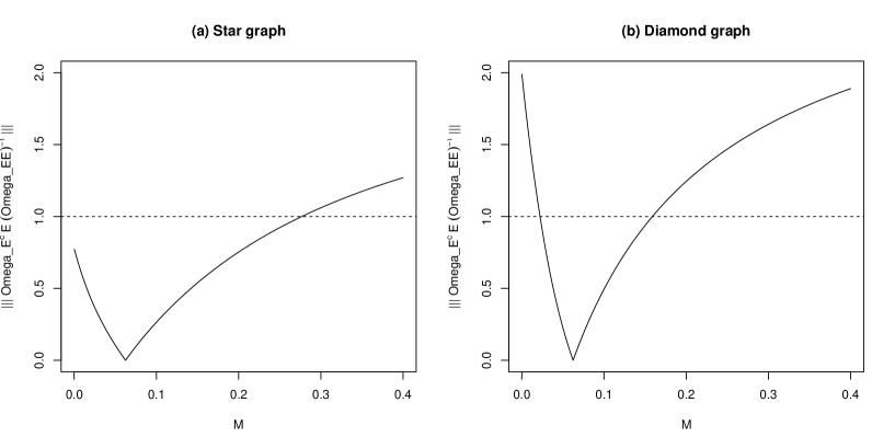
For $d=4$, we investigate two theoretical examples. In particular, we focus on the Mutual Incoherence condition

$$|||\Omega_{E^{c}E}(\Omega_{EE})^{-1}|||_{\infty}<1,$$

and demonstrate how the validity of this condition depends on the choice of $M$.

Figure 1 shows the graph structures for the two examples, the star graph and the diamond graph. The Mutual Incoherence condition for these two graphs in the classical graphical lasso setting was studied in Ravikumar et al. (2011).

Figure 1: (a) Star graph; (b) Diamond graph.

5.1.1 Star graph

Notice that the precision matrix $\Theta$ in the HR model satisfies the constraint $\Theta\mathbf{1}=\mathbf{0}$, which leaves limited options for $\Theta$ given a certain sparsity structure. We consider the following parameterization

$$\Theta=\begin{pmatrix}3&-1&-1&-1\\ -1&1&0&0\\ -1&0&1&0\\ -1&0&0&1\\ \end{pmatrix},$$

which reflects the Star graph in Figure 1(a).

We plot the values of $|||\Omega_{E^{c}E}(\Omega_{EE})^{-1}|||_{\infty}$ against the values of $M$ on the left panel of Figure 2. The figure shows that the Mutual Incoherence condition is satisfied when $M\in(0,0.2768]$.

Figure 2: The curves of $|||\Omega_{E^{c}E}(\Omega_{EE})^{-1}|||_{\infty}$ versus $M$ for the star graph and the diamond graph.

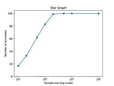
We simulate 100 samples with various sample sizes $n$: ranging from $10^{3}$ to $10^{6}$. For each sample we simulate data from the following multivariate Pareto distribution

$$\mathbf{X}=Y\exp\{\mathbf{W}-\sigma^{2}(\mathbf{W})/2\},$$

where $\mathbf{W}$ follows a zero-mean Gaussian distribution with a covariance matrix $\Sigma$ calculated based on Proposition 3.1, and $Y$ follows a standard Pareto distribution and is independent of $\mathbf{W}$. Here $\sigma^{2}(\mathbf{W})$ is the diagonal vector of $\Sigma$. Note that the choice of $M$ here is irrelevant to the calculation of $\Sigma$ . The multivariate Pareto distribution used in the simulation is in the domain of attraction of a HR model with precision matrix $\Theta$.

We apply the extreme graphical lasso method to estimate the graphical structure of $\Theta$. More specifically, for the estimator $\hat{\Sigma}$, we use $k_{n}=0.05n$. For the extreme graphical lasso, we choose $M=0.25$ which ensures the Mutual Incoherence condition and a penalty parameter $\gamma_{n}=0.2$. Here the optimization problem (3.6) is convex and can be solved with a block coordinate descent algorithm similar to Mazumder and Hastie (2012), see Appendix D.

After obtaining $\hat{\Theta}$ we further consider a thresholding by $0.01$: if an estimated off-diagonal element has an absolute value less or equal to $10^{-2}$, it will be set to zero. The last step is purely for computational reason. For each simulated sample, we consider it as a “success” if the estimated graph coincides with the true graph. The left panel of Figure 3 shows the “success rates” in 100 simulated samples versus the sample sizes.

We observe that the success rate of the extreme graphical lasso method approaches 100% as $n$ increases, indicating that the graph can be consistently identified. Note that here $k_{n}$ is the effective sample size and corresponds to 5% of $n$, e.g. $k_{n}=500$ corresponding to $n=10000$.

(a) Star Graph

(b) Diamond Graph

Figure 3: The success rates vesus sample sizes based on 100 samples

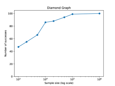
5.1.2 Diamond graph

We now consider the diamond graph in Figure 1(b) corresponding to the following precision matrix

$$\Theta=\begin{pmatrix}2&-1&-1&0\\ -1&3&-1&-1\\ -1&-1&3&-1\\ 0&-1&-1&2\\ \end{pmatrix}.$$

Again we plot the values of $|||\Omega_{E^{c}E}(\Omega_{EE})^{-1}|||_{\infty}$ against the values of $M$ on the right panel of Figure 2. The figure shows that the Mutual Incoherence condition is satisfied when $M\in[0.0224,0.1588]$.

We conduct simulations for the diamond graph with the same setup as in Section 5.1.1. In the extreme graphical lasso estimation, we choose $M=0.15$ and $\gamma_{n}=0.1$. The results for the success rate are shown on the right panel of Figure 3. Again the graph structure can be consistently identified for sample sizes starting from $n=5000$ corresponding to an effect sample size $k_{n}=250$. Compared to identifying the Star graph, identifying the Diamond graph is relatively easier.

5.2 Simulations in high dimensional cases ($d=20$ and $d=200$)

We demonstrate the performance of the extreme graphical lasso method in higher dimensional situations.

If the dimension $d$ is high, the extreme graphical lasso method can be simplified to a standard graphical lasso method as follows. Recall the extreme graphical lasso procedure in (3.6) and (3.7). In the optimization step, we shrink off-diagonal entries of the matrix $\Theta^{*}$ towards $\frac{1}{d^{2}M}$. When $d$ is large, the term $\frac{1}{d^{2}M}$ is close to zero. Therefore, we can replace the optimization step (3.6) by

$$\hat{\Theta}_{mlasso}:={\arg\min}_{\Theta^{*}}\left\{-\log|\Theta^{*}|+tr\left(S^{*}\Theta^{*}\right)+\gamma_{n}\sum_{i\neq j}\left|\Theta^{*}_{ij}\right|\right\},$$

potentially with a diffrerent penalization parameter $\gamma_{n}$. This practical proposal performs the classical graphical lasso procedure only once. In the estimation, we use the R package glasso in Friedman et al. (2008) for the optimization. We term it as the modified extreme graphical lasso method.

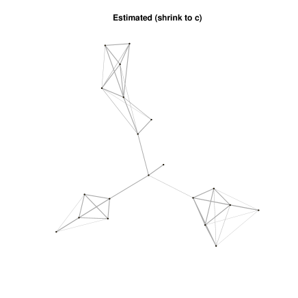
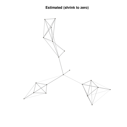
We first demonstrate that the modified extreme graphical lasso procedure results in similar graphs as the extreme graphical lasso method for $d=20$. For that purpose, we simulate observations following a multivariate Pareto distribution with $d=20$. The multivariate Pareto distribution is in the domain of attraction of a HR model with a specific precision matrix goverend by a graph. The true graph is presimulated by a preferential attach model as in Albert and Barabási (2002), see Figure 4(a). Given the graph, the simulation of the observations is achieved by using the R package graphicalExtremes in Engelke and Hitz (2020). We simulate 100 samples with sample size 5000.

Across the 100 samples, we apply the extreme graphical lasso method to estimate the graph structure with $k_{n}=250$, $M=1$ and $\gamma_{n}=2.4$. In the extreme graphical lasso method, we shrink the off-diagonal elements of $\hat{\Theta}^{*}$ towards $c=1/(d^{2}M)$. For each pair of nodes, we count the number of samples for which an edge is identified. Figure 4(b) shows the aggregation of 100 estimated graphs, where the thickness of each edge reflects the proportion of times an edge is identified.

Next, we apply the modified extreme graphical lasso method based on the same estimated $\Sigma$. Here we use $\gamma_{n}=1.2$. The aggregation of 100 estimated graphs is shown in Figure 4(c).

The two graphs in the panels (b) and (c) of Figure 4 are virtually the same, with the modified procedure identifying slightly more wrong edges. Both graphs are comparable with the true graph in panel (a), indicating the applicability of both procedures.

(a) True Graph

(b) Estimated Graph: extreme graphical lasso

(c) Estimated Graph: modified procedure

Figure 4: The true and estimated graphs for $d=20$ (100 samples)

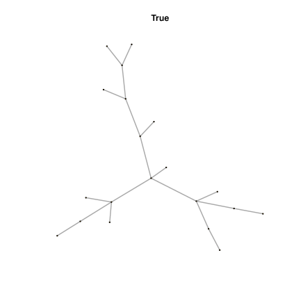
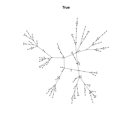
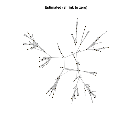
Now we demonstrate the efficiency of the modified extreme graphical lasso in a very high dimensional case $d=200$. We perform a simulation for $d=200$ with $n=100000$. The simulation setup is similar to the $d=20$ case, while in the estimation we use the modified extreme graphical lasso procedure with $k_{n}=5000$ and $\gamma_{n}=1.9$. Here the penalization parameter is chosen at the highest level for which the estimated graph is connected. The true graph and the aggretaged graph from 10 simulations are shown in Figure 5.

We particularly focus on the efficiency of the algorithm. The average time for running each of the 10 iteration is 3.23 min. Per iteration, the majority time is devoted to simulating the data (0.378 min) and estimating the $\Sigma$ matrix (2.848 min), while the time to perform the modified extreme graphical lasso method is only 0.0037 min, about 0.22 second. Considering that this is for $d=200$, the modified extreme graphical lasso method has great potential for handling even higher dimensional cases.

(a) True Graph

(b) Estimated Graph

Figure 5: The true and estimated graphs for $d=200$ (10 samples)

5.3 Real data example: river discharge

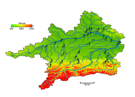
We apply the modified extreme graphical lasso method to the river discharge data in the upper Danube basin. This dataset was first analyzed in Asadi et al. (2015) and subsequently studied in Engelke and Hitz (2020). The data contain river discharge at $d=31$ stations with a sample size $428$ after declustering. The physical locations of the stations and the altitude of the area are shown in Figure 6. We refer interested readers to Asadi et al. (2015) for more information about the dataset and the declustering procedure. We use $k_{n}=64$ in the estimation, and vary the penalization parameter $\gamma_{n}$ to obtain different estimated graphs.

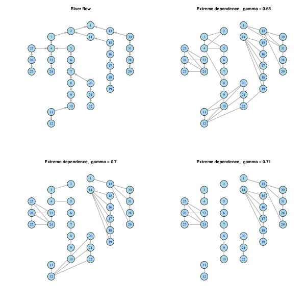
In Figure 7, the top left panel shows the physical connection of the stations following the Danube basin. The other three panels in the figure show different estimated graphs using different values of $\gamma_{n}$. With increasing $\gamma_{n}$ the estimated graph contains fewer edges and eventually turns to disconnected graphs. Nevertheless, such a graph will be useful for practitioners to understand the most related extreme river discharge across the stations.

For instance, we observe that the extreme river discharge at Station 1 is more related to the stream from Station 13, intead of the other stream from Station 2. The stream from Station 13 is the downstrem of the river Salzach, originally starting in the Alps, while the stream from Station 2 is the Danube river flowing over a plain area. Similarly, the extreme river discharge at Station 2 is more related to the main stream from Station 3 (the Danube river) instead of the branch from Station 14 (the Isar river).

To conclude, by applying the (modified) extreme graphical lasso method to the Danube river discharge data, we obtain insights regarding the interrelations of extreme river discharges at a large number of stations spanning in a large spatial area.

Figure 6: The river map of the upper Danube basin. Courtesy of Asadi et al. (2015).

Figure 7: The physical flow connection and estimated graphs for the Danube river discharge data.

Appendix A Proof of propositions in Sections 3

We first prove Proposition 3.2 and then use the result to prove Proposition 3.1.

Proof of Proposition 3.2.

Note that the $(i,j)$th element of $\frac{1}{d}\sum_{k=1}^{d}\tilde{\Sigma}^{(k)}$ is equal to

$$\left(\frac{1}{d}\sum_{k=1}^{d}\tilde{\Sigma}^{(k)}\right)_{i,j} = \frac{1}{2}\frac{1}{d}\sum_{k=1}^{d}(\Gamma_{ik}+\Gamma_{jk}-\Gamma_{ij})$$

$$= -\frac{1}{2}\left(\Gamma_{ij}-\frac{1}{d}\sum_{k=1}^{d}\Gamma_{ik}-\frac{1}{d}\sum_{k=1}^{d}\Gamma_{jk}\right).$$

Hence

$$\frac{1}{d}\sum_{k=1}^{d}\tilde{\Sigma}^{(k)} = -\frac{1}{2}\left(\Gamma-\frac{1}{d}\Gamma\mathbf{1}\mathbf{1}^{T}-\frac{1}{d}\mathbf{1}\mathbf{1}^{T}\Gamma\right)$$

$$= -\frac{1}{2}\left(\Gamma-\frac{1}{d}\Gamma\mathbf{1}\mathbf{1}^{T}-\frac{1}{d}\mathbf{1}\mathbf{1}^{T}\Gamma+\frac{1}{d^{2}}\mathbf{1}\mathbf{1}^{T}\Gamma\mathbf{1}\mathbf{1}^{T}\right)+\frac{1}{2d^{2}}\mathbf{1}\mathbf{1}^{T}\Gamma\mathbf{1}\mathbf{1}^{T}$$

$$= -\frac{1}{2}\left(I-\frac{\mathbf{1}^{T}\mathbf{1}}{d}\right)\Gamma\left(I-\frac{\mathbf{1}^{T}\mathbf{1}}{d}\right)+\left(\frac{\mathbf{1}^{T}\Gamma\mathbf{1}}{d^{2}}\right)\cdot\mathbf{1}\mathbf{1}^{T}$$

$$= \Sigma+\left(\frac{\mathbf{1}^{T}\Gamma\mathbf{1}}{d^{2}}\right)\cdot\mathbf{1}\mathbf{1}^{T}.$$

Summing up the elements of the matrices on both sides, we have

$$\mathbf{1}^{T}\left(\frac{1}{d}\sum_{k=1}^{d}\tilde{\Sigma}^{(k)}\right)\mathbf{1} = \mathbf{1}^{T}\Sigma\mathbf{1}+\mathbf{1}^{T}\left(\left(\frac{\mathbf{1}^{T}\Gamma\mathbf{1}}{d^{2}}\right)\cdot\mathbf{1}\mathbf{1}^{T}\right)\mathbf{1}$$

$$= 0+\mathbf{1}^{T}\Gamma\mathbf{1}.$$

Plugging in the value for $\mathbf{1}^{T}\Gamma\mathbf{1}$ back into the previous equation, we obtain that

$$\frac{1}{d}\sum_{k=1}^{d}\tilde{\Sigma}^{(k)}=\Sigma+\frac{1}{d^{2}}\mathbf{1}^{T}\left(\frac{1}{d}\sum_{k=1}^{d}\tilde{\Sigma}^{(k)}\right)\mathbf{1}\cdot\mathbf{1}\mathbf{1}^{T}=\Sigma+\frac{1}{d^{3}}\left(\sum_{k=1}^{d}\mathbf{1}^{T}\tilde{\Sigma}^{(k)}\mathbf{1}\right)\cdot\mathbf{1}\mathbf{1}^{T}.$$

∎

Proof of Proposition 3.1.

Using the property $\Sigma\mathbf{1}=\mathbf{0}$ and $\Theta\mathbf{1}=\mathbf{0}$ and the fact that $\Sigma$ and $\Theta$ are both symmetric, we get

$$\left(\Sigma+M\mathbf{1}\mathbf{1}^{T}\right)\cdot\left(\Theta+\frac{1}{d^{2}M}\mathbf{1}\mathbf{1}^{T}\right)$$

$$= \Sigma\cdot\Theta+M\mathbf{1}\mathbf{1}^{T}\cdot\Theta+\Sigma\cdot\frac{1}{d^{2}M}\mathbf{1}\mathbf{1}^{T}+M\mathbf{1}\mathbf{1}^{T}\cdot\frac{1}{d^{2}M}\mathbf{1}\mathbf{1}^{T}$$

$$= \Sigma\cdot\Theta+M\mathbf{1}\cdot\left(\Theta\mathbf{1}\right)^{T}+\frac{1}{d^{2}M}\cdot\Sigma\mathbf{1}\cdot\mathbf{1}^{T}+(M\cdot\frac{1}{d^{2}M})\cdot\mathbf{1}\mathbf{1}^{T}\cdot\mathbf{1}\mathbf{1}^{T}$$

$$= \Sigma\cdot\Theta+\frac{1}{d}\cdot\mathbf{1}\mathbf{1}^{T}$$

From Proposition 3.2, we can write the first term as

$$\Sigma\cdot\Theta = \left(\frac{1}{d}\sum_{k=1}^{d}\tilde{\Sigma}^{(k)}-M_{\Sigma}\mathbf{1}\mathbf{1}^{T}\right)\cdot\Theta$$

$$= \frac{1}{d}\sum_{k=1}^{d}\tilde{\Sigma}^{(k)}\cdot\Theta-M_{\Sigma}\mathbf{1}\mathbf{1}^{T}\cdot\Theta$$

$$= \frac{1}{d}\sum_{k=1}^{d}\tilde{\Sigma}^{(k)}\cdot\Theta$$

$$= I_{d\times d}-\frac{1}{d}\cdot\mathbf{1}\mathbf{1}^{T}.$$

Therefore

$$\left(\Sigma+M\mathbf{1}\mathbf{1}^{T}\right)\cdot\left(\Theta+\frac{1}{d^{2}M}\mathbf{1}\mathbf{1}^{T}\right)=I_{d\times d}.$$

∎

In order to prove Proposition 3.3, we make use of the following lemma.

Lemma A.1.

For any $k$,

$$|\Theta^{*}|=\frac{1}{M}|\Theta^{(k)}|.$$

Proof of Lemma A.1.

We will first show that for $k\neq k^{\prime}$,

$$|\Theta^{(k)}|=|\Theta^{(k^{\prime})}|.$$

Note that

$$\Theta^{(k)}=A_{k}^{T}\Theta A_{k},$$

where $A_{k}\in\mathbb{R}^{d\times(d-1)}$, $A_{k}[,k]={\bf 0}$ and $A_{k}[,-k]=I_{(d-1)\times(d-1)}$. In other words, $A_{k}$ takes the $(d-1)\times(d-1)$ identity matrix and insert an extra $k$-th row with zero entries. On the other hand, we have

$$\Theta=B_{k}\Theta^{(k)}B_{k}^{T},$$

where $B_{k}\in\mathbb{R}^{d\times(d-1)}$, $B_{k}[,k]=-{\mathbf{1}}$ and $B_{k}[,-k]=I_{(d-1)\times(d-1)}$. In other words, $B_{k}$ takes the $(d-1)\times(d-1)$ identity matrix and insert an extra $k$-th row with $-1$ entries. Therefore we have

$$\Theta^{(k^{\prime})}=A_{k^{\prime}}^{T}B_{k}\Theta^{(k)}B_{k}^{T}A_{k^{\prime}}$$

and

$$|\Theta^{(k^{\prime})}|=|A_{k^{\prime}}^{T}B_{k}|\cdot|\Theta^{(k)}|\cdot|B_{k}^{T}A_{k^{\prime}}|.$$

Now we claim that $|A_{k^{\prime}}^{T}B_{k}|=1$ for any $k,k^{\prime}$. We have

$$A_{k^{\prime}}^{T}B_{k} = \sum_{h=1}^{d}A_{k^{\prime}}[,h]^{T}B_{k}[h,]$$

$$= \sum_{h\neq k^{\prime}}A_{k^{\prime}}[,h]^{T}B_{k}[h,]+A_{k^{\prime}}[,k^{\prime}]^{T}B_{k}[k^{\prime},]$$

$$= A_{k^{\prime}}[,-k^{\prime}]^{T}B_{k}[-k^{\prime},]+A_{k^{\prime}}[,k^{\prime}]^{T}B_{k}[k^{\prime},]$$

$$= I_{(d-1)\times(d-1)}B_{k}[-k^{\prime},]+{\bf 0}^{T}B_{k}[k^{\prime},]$$

$$= B_{k}[-k^{\prime},].$$

For example, assume that $k=1$ and $k^{\prime}=d$, then

$$B_{1}[-d,]=\left(\begin{array}[]{ccccc}-1&-1&\cdots&-1&-1\\ 1&0&\cdots&0&0\\ 0&1&\cdots&0&0\\ \vdots&\vdots&\vdots&\vdots&\vdots\\ 0&0&\cdots&1&0\\ \end{array}\right)$$

and it is easy to see that $|B_{1}[-d,]|=1$.

It can be shown by the calculation of determinant that $|B_{k}[-k^{\prime},]|=1$ for any $k\neq k^{\prime}$. Therefore

$$|A_{k^{\prime}}^{T}B_{k}|=1,\quad k\neq k^{\prime},$$

and

$$|\Theta^{(k)}|=|\Theta^{(k^{\prime})}|,\quad k\neq k^{\prime}.$$

Now to show that $|\Theta^{*}|=\frac{1}{M}|\Theta^{(k)}|$, it suffices to prove it for one value of $k$. We will show it for $k=d$.

Note that we have

$$\frac{1}{M}|\Theta^{(d)}|=\left|\left(\begin{array}[]{cc}\Theta^{(d)}&{\bf 0}\\ {\bf 0}^{T}&\frac{1}{M}\end{array}\right)\right|.$$

We establish the following transformation

$$\left(\begin{array}[]{cc}I&{\bf 0}\\ -\mathbf{1}^{T}&1\end{array}\right)\left(\begin{array}[]{cc}I&\frac{1}{d}\mathbf{1}\\ {\bf 0}^{T}&1\end{array}\right)\left(\begin{array}[]{cc}\Theta^{(d)}&{\bf 0}\\ {\bf 0}^{T}&\frac{1}{M}\end{array}\right)\left(\begin{array}[]{cc}I&{\bf 0}\\ \frac{1}{d}\mathbf{1}^{T}&1\end{array}\right)\left(\begin{array}[]{cc}I&-\mathbf{1}\\ {\bf 0}^{T}&1\end{array}\right)$$

$$= \left(\begin{array}[]{cc}I&{\bf 0}\\ -\mathbf{1}^{T}&1\end{array}\right)\left(\begin{array}[]{cc}\Theta^{(d)}+\frac{1}{d^{2}M}\mathbf{1}\mathbf{1}^{T}&\frac{1}{dM}{\bf 1}\\ \frac{1}{dM}{\bf 1}^{T}&\frac{1}{M}\end{array}\right)\left(\begin{array}[]{cc}I&-\mathbf{1}\\ {\bf 0}^{T}&1\end{array}\right)$$

$$= \left(\begin{array}[]{cc}\Theta^{(d)}+\frac{1}{d^{2}M}\mathbf{1}\mathbf{1}^{T}&-\Theta^{(d)}\mathbf{1}+\frac{1}{d^{2}M}{\bf 1}\\ -\mathbf{1}^{T}\Theta^{(d)}+\frac{1}{d^{2}M}{\bf 1}^{T}&\mathbf{1}^{T}\Theta^{(d)}\mathbf{1}+\frac{1}{d^{2}M}\end{array}\right)$$

$$= \Theta+\frac{1}{d^{2}M}\mathbf{1}\mathbf{1}^{T}$$

$$= \Theta^{*}.$$

Since

$$\left|\left(\begin{array}[]{cc}I&{\bf 0}\\ -\mathbf{1}^{T}&1\end{array}\right)\right|=\left|\left(\begin{array}[]{cc}I&{\bf 0}\\ \frac{1}{d}\mathbf{1}^{T}&1\end{array}\right)\right|=1,$$

we have

$$|\Theta^{*}|=\left|\left(\begin{array}[]{cc}\Theta^{(d)}&{\bf 0}\\ {\bf 0}^{T}&\frac{1}{M}\end{array}\right)\right|=\frac{1}{M}|\Theta^{(d)}|.$$

∎

Proof of Proposition 3.3.

The aggregated negative log-likelihood function can be written as

$$\frac{1}{d}\sum_{k=1}^{d}\left\{-\log|\Theta^{(k)}|+tr\left(S_{k}\Theta^{(k)}\right)\right\}$$

$$= \frac{1}{d}\sum_{k=1}^{d}\left\{-\log|\Theta^{(k)}|+tr\left(\tilde{S}_{k}\Theta\right)\right\}$$

$$= \frac{1}{d}\sum_{k=1}^{d}\left\{-\log|\Theta^{(k)}|\right\}+tr\left(\left(\frac{1}{d}\sum_{k=1}^{d}\tilde{S}_{k}\right)\Theta\right)$$

$$= -\log|\Theta^{*}|+\log(M)+tr\left(\left(\frac{1}{d}\sum_{k=1}^{d}\tilde{S}_{k}-\left(\frac{1}{d^{3}}\sum_{k=1}^{d}{\mathbf{1}^{T}\tilde{S}_{k}\mathbf{1}}\right)\mathbf{1}\mathbf{1}^{T}+M\cdot\mathbf{1}\mathbf{1}^{T}\right)\Theta\right)$$

$$= -\log|\Theta^{*}|+\log(M)+tr\left(S^{*}\left(\Theta^{*}-\frac{1}{d^{2}M}\mathbf{1}\mathbf{1}^{T}\right)\right).$$

∎

Appendix B Proof of Proposition 4.1

Proof of Proposition 4.1.

We intend to apply Theorem 3 in Engelke et al. (2022). For that purpose, we first verify all assumptions needed for that theorem, namely Assumptions 1 and 2 therein.

We handle Assumption 1 first. Based on Lemma S3 in Engelke et al. (2022), Condition 4.2 implies that for any $\xi^{\prime\prime}>0$, there exists $K_{\xi^{\prime\prime}}>0$ depending on $\underline{\lambda}$ and $\overline{\lambda}$, but independent of $d$, such that Assumption 4 therein holds. Denote $K=K^{\prime}+2K_{\xi^{\prime\prime}}$ and $\xi=\xi^{\prime}\xi^{\prime\prime}/(1+\xi^{\prime}+\xi^{\prime\prime})$. Together with Condition 4.1, we get that Assumption 1 in Engelke et al. (2022) holds. In particular, one can choose $\xi^{\prime\prime}$ sufficiently large such that $\xi$ can be any constant satisfying $\xi<\xi^{\prime}$.

Next, Assumption 2 in Engelke et al. (2022) holds automatically for all non-degenerate HR distribution satisfying our Condition 4.2. Therefore, we can then apply Theorem 3 therein to obtain that there exists positive constants $C_{1}$, $C_{2}$ and $C_{3}$, independent of $d$, such that for any $k_{n}\geq n^{\xi}$ and $\lambda\leq\sqrt{k_{n}}/(\log n)^{4}$,

$$\mathbb{P}\left(\max_{1\leq k\leq d}\|\hat{\Sigma}^{(k)}-\Sigma^{(k)}\|_{\infty}>C_{1}\left\{\left(\frac{k_{n}}{n}\right)^{\xi}\left(\log\left(\frac{k_{n}}{n}\right)\right)^{2}+\frac{1+\lambda}{\sqrt{k_{n}}}\right\}\right)\leq C_{2}d^{3}e^{-C_{3}\lambda^{2}}.$$ (B.1)

Notice that the constant $C_{1}$ here equals to $\frac{3}{2}\overline{C}$ in Theorem 3 in Engelke et al. (2022) because we are estimating the matrix $\Sigma$ instead of the variogram $\Gamma$.

For any $\varepsilon\geq C_{2}d^{3}\exp\{-\frac{C_{3}k_{n}}{(\log n)^{8}}\}$, one can choose $\lambda=\sqrt{\frac{1}{C_{3}}\log(C_{2}d^{3}/\varepsilon)}\leq\frac{\sqrt{k_{n}}}{(\log n)^{4}}$ in (B.1) to obtain the element-wise bound for the estimation error $\hat{\Sigma}^{(k)}-\Sigma^{(k)}$ uniformly for all $1\leq k\leq d$.

Since

$$S-\Sigma=\frac{1}{d}\sum_{k=1}^{d}(\hat{\Sigma}^{(k)}-\Sigma^{(k)})-\frac{1}{d}\sum_{k=1}^{d}\left(\frac{1}{d^{2}}\mathbf{1}^{T}(\hat{\Sigma}^{(k)}-\Sigma^{(k)})\mathbf{1}\right)\mathbf{1}\mathbf{1}^{T},$$

which implies that $\|S-\Sigma\|_{\infty}\leq 2\max_{1\leq k\leq d}\|\hat{\Sigma}^{(k)}-\Sigma^{(k)}\|_{\infty}$, we immediately get the inequality (4.1) with replacing $C_{1}$ by $2C_{1}$. W.l.o.g., we continue using $C_{1}$.

For the asymptotic statement, note that if $(\log n)^{4}\sqrt{\frac{\log d}{k_{n}}}\to 0$ as $n\to\infty$, then the lower bound for $\varepsilon$, $\varepsilon_{n}\to 0$ as $n\to\infty$. The asymptotic statement follows immediately. ∎

Appendix C Proof of Theorem 4.2

Proof of Theorem 4.2.

We shall work with the event

$$A_{\varepsilon}=\{\|S-\Sigma\|_{\infty}<\delta_{n}\},$$

which satisfies $\mathbb{P}(A_{\varepsilon})>1-\varepsilon$ following Proposition 4.1. Denote $c:=\frac{1}{d^{2}M}.$ Then

$$\Theta^{*}=\Theta+c\mathbf{1}\mathbf{1}^{T}.$$

Here we omit $M$ in the notation for simplicity.

Recall that $\hat{\Theta}^{*}$ is the solution to the following graphical lasso problem

$$\hat{\Theta}^{*}:={\arg\min}_{\Theta^{*}}\left\{-\log|\Theta^{*}|+tr(S^{*}\Theta^{*})+\gamma_{n}\sum_{i\neq j}|\Theta^{*}_{ij}-c|\right\}$$

and $\hat{\Theta}_{lasso}:=\hat{\Theta}^{*}-c\mathbf{1}\mathbf{1}^{T}$. The estimated edge set is $\hat{E}:=\{(i,j):\hat{\Theta}_{lasso,ij}\neq 0\}.$

We aim to prove that on $A_{\varepsilon}$, $\hat{E}\subset E,$ and

$$\|\hat{\Theta}_{lasso}-\Theta\|_{\infty}\leq r_{n},$$

which is equivalent to proving

$$\|\hat{\Theta}^{*}-\Theta^{*}\|_{\infty}\leq r_{n}.$$

We first show that the solution $\hat{\Theta}^{*}$ exsits and is unique. The proof follows the same lines as that for Lemma 3 in Ravikumar et al. (2011). Note that the estimator $S^{*}$ is positive definite with all diagonal elements being positive. The rest of the proof follows exactly the same arguments therein.

Next, the solution $\hat{\Theta}^{*}$ must satisfy the following KKT condition.

$$-\left(\hat{\Theta}^{*}\right)^{-1}+S^{*}+\gamma_{n}\hat{Z}=0,$$ (C.1)

where

$$\hat{Z}_{ij}=\begin{cases}0&\text{ if }i=j,\\ \text{sign}(\hat{\Theta}^{*}_{ij}-c)&\text{ if }i\neq j\text{ and }\hat{\Theta}^{*}_{ij}\neq c,\\ \in[-1,1]&\text{ if }i\neq j\text{ and }\hat{\Theta}^{*}_{ij}=c.\end{cases}$$

We shall construct a “witness” precision matrix $\tilde{\Theta}^{*}$ as follows. Let $\tilde{\Theta}^{*}$ be the solution to the following optimization problem,

$$\tilde{\Theta}^{*}:={\arg\min}_{\{\Theta^{*}:\Theta^{*}_{ij}=c,(i,j)\in E^{c}\}}-\log|\Theta^{*}|+tr(S^{*}\Theta^{*})+\gamma_{n}\sum_{i\neq j}|\Theta^{*}_{ij}-c|.$$ (C.2)

This is the same optimization but constrained to a smaller domain. Let $\tilde{E}$ denote the graph recovered from $\tilde{\Theta}^{*}$. Clearly, $\tilde{\Theta}^{*}$ satisfies: $\tilde{\Theta}^{*}_{ij}=c$ for $(i,j)\in E^{c}$, i.e. $\tilde{E}\subset E$.

We shall show that under the conditions in Theorem 4.2,

• $\tilde{\Theta}^{*}$ satisfies the above KKT condition;

• $\|\tilde{\Theta}^{*}-\Theta^{*}\|_{\infty}\leq r_{n}$.

Then by uniqueness, $\tilde{\Theta}^{*}=\hat{\Theta}^{*}$ and satisfies the goal that we are aiming to prove.

With a similar argument regarding the existence and uniqueness of the original optimization problem, the solution to the problem (C.2) also exists and is unique. In addition, it satisfies a similar KKT condition as follows,

$$-\left(\tilde{\Theta}^{*}\right)^{-1}_{ij}+S^{*}_{ij}+\gamma_{n}\tilde{Z}_{ij}=0,\quad(i,j)\in E,$$

where

$$\tilde{Z}_{ij}=\begin{cases}\text{sign}(\tilde{\Theta}^{*}_{ij}-c)&\text{if }\tilde{\Theta}^{*}_{ij}\neq c,\\ \in[-1,1]&\text{if }\tilde{\Theta}^{*}_{ij}=c.\end{cases}$$

Note that this coincides with the KKT condition (C.1), but only on entries indexed by $E$. As a matter of fact, $\tilde{Z}$ is only defined on $E$. In order to argue $\tilde{\Theta}^{*}$ as a candidate for $\hat{\Theta}^{*}$ and satisfies the full KKT condition, we will now extend the definition of $\tilde{Z}$ to $E^{c}$ as well.

Define

$$\tilde{Z}_{ij}:=\frac{1}{\gamma_{n}}\left(\left(\tilde{\Theta}^{*}\right)^{-1}_{ij}-S^{*}_{ij}\right),\quad(i,j)\notin E.$$

Then the pair $(\tilde{\Theta}^{*},\tilde{Z})$ satisfies the original KKT equation (C.1). What remains to be proved is that $\tilde{Z}$ also satisfies

$$|\tilde{Z}_{ij}|\leq 1,\quad(i,j)\notin E.$$

To summarize, in order to complete the proof of Theorem 4.2, we will show that on the set $A_{\varepsilon}$,
Goal 1: $|\tilde{Z}_{ij}|\leq 1,\quad(i,j)\notin E.$
Goal 2: $\|\tilde{\Theta}^{*}-\Theta^{*}\|_{\infty}\leq r_{n}$.

In the rest of the proof we denote

$$\Delta:=\tilde{\Theta}^{*}-\Theta^{*}.$$

Note that for $(i,j)\notin E$, $\tilde{\Theta}_{ij}=c$ by definition and $\Theta_{ij}=c$. Therefore, $\Delta_{E^{c}}=\mathbf{0}$ and Goal 2 above can be translated to

$$\|\Delta_{E}\|_{\infty}\leq r_{n}.$$

To handle the KKT condition for $\tilde{\Theta}^{*}$, we start with handling $\left(\tilde{\Theta}^{*}\right)^{-1}$ as follows:

$$\left(\tilde{\Theta}^{*}\right)^{-1} = \left(\Theta^{*}+\Delta\right)^{-1}$$

$$= \left(\Theta^{*}(I+\Sigma^{*}\Delta)\right)^{-1}$$

$$= (I+\Sigma^{*}\Delta)^{-1}\Sigma^{*}=:J\Sigma^{*}.$$

Now in the case where $|||\Sigma^{*}\Delta|||_{\infty}<1$, we can expand $J$ as

$$J=\sum_{k=0}^{\infty}(-1)^{k}(\Sigma^{*}\Delta)^{k}=I-\Sigma^{*}\Delta+(\Sigma^{*}\Delta)^{2}J.$$

Inspired from this relation, we can use $\Sigma^{*}-\Sigma^{*}\Delta\Sigma^{*}$ to approximate $\left(\tilde{\Theta}^{*}\right)^{-1}$ and define

$$R:=\left(\tilde{\Theta}^{*}\right)^{-1}-(\Sigma^{*}-\Sigma^{*}\Delta\Sigma^{*}),$$

as the approximation error. Note that $R$ is defined regardless of whether $|||\Sigma^{*}\Delta|||_{\infty}<1$.

Recall that $\Sigma^{*}=\Sigma+M\mathbf{1}\mathbf{1}^{T}$ and $S^{*}=S+M\mathbf{1}\mathbf{1}^{T}$. Define

$$R^{\prime}:=S^{*}-\Sigma^{*}=S-\Sigma.$$

On the set $A_{\varepsilon}$, we have that $\|R^{\prime}\|_{\infty}\leq\delta_{n}$.

Rewrite the KKT condition as

$$\Sigma^{*}\Delta\Sigma^{*}-R+R^{\prime}+\gamma_{n}\tilde{Z}=0.$$

We vectorize it using the notation $\bar{\cdot}$ as the vectorization of a matrix. Then the vectorized KKT condition is

$$\overline{\Sigma^{*}\Delta\Sigma^{*}}-\overline{R}+\overline{R^{\prime}}+\gamma_{n}\overline{\tilde{Z}}=0.$$

Note that

$$\overline{\Sigma^{*}\Delta\Sigma^{*}}=(\Sigma^{*}\otimes\Sigma^{*})\overline{\Delta}=:\Omega\overline{\Delta},$$

where $\Omega:=\Sigma^{*}\otimes\Sigma^{*}$ denotes the Kronecker product of $\Sigma^{*}$ with itself. Then we have

$$\Omega\overline{\Delta}-\overline{R}+\overline{R^{\prime}}+\gamma_{n}\overline{\tilde{Z}}=0.$$

By examining the rows of $\Omega$ indexed by $E$ and $E^{c}$ separately and noting that $\Delta_{E^{c}}=0$, we get

$$\Omega_{EE}\overline{\Delta}_{E}-\overline{R}_{E}+\overline{R^{\prime}}_{E}+\gamma_{n}\overline{\tilde{Z}}_{E}=0,$$ (C.3)

$$\Omega_{E^{c}E}\overline{\Delta}_{E}-\overline{R}_{E^{c}}+\overline{R^{\prime}}_{E^{c}}+\gamma_{n}\overline{\tilde{Z}}_{E^{c}}=0.$$ (C.4)

Proof of Goal 2

To prove Goal 2, we shall show that for any pre-specified $\|\tilde{Z}_{E}\|_{\infty}\leq 1$, there exists a solution to $\Delta$ which satisfies:

• $-\left(\Theta^{*}+\Delta\right)^{-1}_{E}+S^{*}_{E}+\gamma_{n}\tilde{Z}_{E}=0$;

• $\Delta_{E^{c}}=\mathbf{0}$;

• $\|\Delta_{E}\|_{\infty}\leq r_{n}$.

With the statement above proven, given the $\tilde{Z}_{E}$ produced from the KKT condition for $\tilde{\Theta}^{*}$, a solution $\Delta$ exists and coincides with $\tilde{Z}_{E}$. Then this is the unique solution. Hence $\|\tilde{\Theta}^{*}-\Theta^{*}\|_{\infty}\leq r_{n}$ which concludes Goal 2.

Now we construct such a solution $\Delta$. Recall that $\Delta_{E^{c}}=\mathbf{0}$, we only need to construct a suitable $\Delta_{E}$ by utilizing the Brouwer fixed point theorem.

The solution $\Delta_{E}$ satisfies (C.3), which can be rewritten as

$$\overline{\Delta}_{E}=(\Omega_{EE})^{-1}\left(\overline{R}_{E}-\overline{R^{\prime}}_{E}-\gamma_{n}\overline{\tilde{Z}}_{E}\right).$$

We regard

$$R=\left(\tilde{\Theta}^{*}\right)^{-1}-(\Sigma^{*}-\Sigma^{*}\Delta\Sigma^{*})$$

as a function of $\Delta$ or eventually a function of $\overline{\Delta}_{E}$. To stress this point we define it as $R=R(\Delta_{E})$. Also recall that $R^{\prime}=S^{*}-\Sigma^{*}$ does not depend on $\overline{\Delta}_{E}$. Then we can write the above equation as

$$\overline{\Delta}_{E}=(\Omega_{EE})^{-1}\left(\overline{R}_{E}(\overline{\Delta}_{E})-\overline{R^{\prime}}_{E}-\gamma_{n}\overline{\tilde{Z}}_{E}\right):=F(\overline{\Delta}_{E}).$$

Consider the closed ball $B(r_{n});=\{x\in\mathbb{R}^{|E|}:\|x\|_{\infty}\leq r_{n}\}$. If $F$ is a continuous mapping from $B(r_{n})$ onto itself, then there exists a fixed point $\overline{\Delta}_{E}$ on $B(r_{n})$ such that $\overline{\Delta}_{E}=F(\overline{\Delta}_{E})$ following the Brouwer fixed point theorem. This is exactly the desired solution. Since $F$ is clearly continuous, we only need to show that $F$ projects $B(r_{n})$ onto itself, that is, for any $\overline{\Delta}_{E}$ satisfying $\|\overline{\Delta}_{E}\|_{\infty}\leq r_{n}$, we have $\|F(\overline{\Delta}_{E})\|_{\infty}\leq r_{n}$.

Assume that $\|\overline{\Delta}_{E}\|_{\infty}\leq r_{n}$. We write

$$\|F(\overline{\Delta}_{E})\|_{\infty}\leq|||(\Omega_{EE})^{-1}|||_{\infty}\left(\|R\|_{\infty}+\|R^{\prime}\|_{\infty}+\gamma_{n}\|\overline{\tilde{Z}}_{E}\|_{\infty}\right)\leq|||(\Omega_{EE})^{-1}|||_{\infty}\left(\|R\|_{\infty}+\|R^{\prime}\|_{\infty}+\gamma_{n}\right),$$

due to the fact that $\|\overline{\tilde{Z}}_{E}\|_{\infty}\leq 1$

We first handle $\|R\|_{\infty}$. Recall that

$$R:=\left(\tilde{\Theta}^{*}\right)^{-1}-(\Sigma^{*}-\Sigma^{*}\Delta\Sigma^{*})=\sum_{k=2}^{\infty}(-1)^{k}(\Sigma^{*}\Delta)^{k}\Sigma^{*}=(\Sigma^{*}\Delta)^{2}J\Sigma^{*},$$

where

$$J=(I+\Sigma^{*}\Delta)^{-1}=\sum_{k=0}^{\infty}(-1)^{k}(\Sigma^{*}\Delta)^{k},$$

provided that $|||\Sigma^{*}\Delta|||_{\infty}<1$. To ensure this condition, note that

$$|||\Sigma^{*}\Delta|||_{\infty}=|||\Sigma^{*}(\tilde{\Theta}-\Theta)|||_{\infty}\leq D|||\Sigma^{*}|||_{\infty}\cdot r_{n},$$

where $D$ is the maximum degree in the graph. Therefore $|||\Sigma^{*}\Delta|||_{\infty}<1$ holds by requiring that

$$D|||\Sigma^{*}|||_{\infty}\cdot r_{n}\leq C_{4}<1.$$ (C.5)

The upper bound $C_{4}$ implies that $|||J^{T}|||_{\infty}\leq\frac{1}{1-C_{4}}.$

With the condition (C.5), we can further derive an upper bound for $\|R\|_{\infty}$. Consider one specific element in $R$. With denoting $\mathbf{e}_{i}$ as a vector with all zero elements except a one element at the $i-$th dimension, we have that

$$R_{ij}=\mathbf{e}_{i}^{T}(\Sigma^{*}\Delta)^{2}J\Sigma^{*}\mathbf{e}_{j}\leq\|\mathbf{e}_{i}^{T}(\Sigma^{*}\Delta)^{2}\|_{\infty}\|J\Sigma^{*}\mathbf{e}_{j}\|_{1}\leq\|(\Sigma^{*}\Delta)^{2}\|_{\infty}|||\Sigma^{*}J^{T}|||_{\infty}.$$

By considering all possible $(i,j)$ we get that,

$$\|R\|_{\infty} \leq \|(\Sigma^{*}\Delta)^{2}\|_{\infty}|||\Sigma^{*}J^{T}|||_{\infty}$$

$$\leq |||\Sigma^{*}\Delta|||_{\infty}\|\Sigma^{*}\Delta\|_{\infty}|||J^{T}|||_{\infty}|||\Sigma^{*}|||_{\infty}$$

$$\leq D|||\Sigma^{*}|||_{\infty}\cdot r_{n}\cdot|||\Sigma^{*}|||_{\infty}r_{n}\cdot\frac{1}{1-C_{4}}\cdot|||\Sigma^{*}|||_{\infty}$$

$$< C_{5}\cdot r_{n}^{2},$$

where $C_{5}=\frac{D}{1-C_{4}}|||\Sigma^{*}|||_{\infty}^{3}$.

Next, since $R^{\prime}=S^{*}-\Sigma^{*}=S-\Sigma,$ we have that on $A_{\varepsilon}$, $\|R^{\prime}\|_{\infty}\leq\delta_{n}.$ Combining the upper bounds for $\|R\|_{\infty}$ and $\|R^{\prime}\|_{\infty}$, we get that on $A_{\varepsilon}$,

$$\|F(\Delta_{E})\|_{\infty}\leq|||(\Omega_{EE})^{-1}|||_{\infty}(C_{5}\cdot r^{2}_{n}+\delta_{n}+\gamma_{n})\leq r_{n},$$

by requiring that

$$C_{5}\cdot r_{n}^{2}+\delta_{n}+\gamma_{n}\leq\frac{1}{|||(\Omega_{EE})^{-1}|||_{\infty}}\cdot r_{n}$$ (C.6)

If the two required conditions (C.5) and (C.6) hold, we achieve Goal 2 by utilizing the Brouwer fixed point theorem.

Proof of Goal 1

To prove Goal 1, we shall show that with the constructed soluition above, we have

$$\|\overline{\tilde{Z}}_{E^{c}}\|_{\infty}\leq 1.$$

We rewrite the equation (C.4) as

$$\overline{\tilde{Z}}_{E^{c}}=-\frac{1}{\gamma_{n}}\Omega_{EE^{c}}\overline{\Delta}_{E}+\frac{1}{\gamma_{n}}\overline{R}_{E^{c}}-\frac{1}{\gamma_{n}}\overline{R^{\prime}}_{E^{c}},$$

and the substitute $\overline{\Delta}_{E}$ above using (C.3) to get that

$$\overline{\tilde{Z}}_{E^{c}}=-\frac{1}{\gamma_{n}}\Omega_{EE^{c}}(\Omega_{EE})^{-1}\left(-\overline{R}_{E}+\overline{R^{\prime}}_{E}+\gamma_{n}\overline{\tilde{Z}}_{E}\right)+\frac{1}{\gamma_{n}}\overline{R}_{E^{c}}-\frac{1}{\gamma_{n}}\overline{R^{\prime}}_{E^{c}}.$$

The upper bound for $\|\overline{\tilde{Z}}_{E^{c}}\|_{\infty}$ is then

$$\|\overline{\tilde{Z}}_{E^{c}}\|_{\infty}\leq\frac{1}{\gamma_{n}}|||\Omega_{EE^{c}}(\Omega_{EE})^{-1}|||_{\infty}\left(\|R\|_{\infty}+\|R^{\prime}\|_{\infty}+\gamma_{n}\|\overline{\tilde{Z}}_{E}\|_{\infty}\right)+\frac{1}{\gamma_{n}}\|R\|_{\infty}+\frac{1}{\gamma_{n}}\|R^{\prime}\|_{\infty}.$$

Using the same upper bounds derived in the proof of Goal 2, we have

$$\|\overline{\tilde{Z}}_{E^{c}}\|_{\infty} \leq \frac{1}{\gamma_{n}}|||\Omega_{EE^{c}}(\Omega_{EE})^{-1}|||_{\infty}\left(\delta_{n}+C_{5}\cdot r_{n}^{2}+\gamma_{n}\right)+\frac{1}{\gamma_{n}}(\delta_{n}+C_{5}\cdot r_{n}^{2})$$

$$= |||\Omega_{EE^{c}}(\Omega_{EE})^{-1}|||_{\infty}+\frac{1}{\gamma_{n}}\left(|||\Omega_{EE^{c}}(\Omega_{EE})^{-1}|||_{\infty}+1\right)\left(\delta_{n}+C_{5}\cdot r_{n}^{2}\right).$$

Since Condition (4.3) ensures that $|||\Omega_{EE^{c}}(\Omega_{EE})^{-1}|||_{\infty}<1-\alpha$, To satisfy $\|\overline{\tilde{Z}}_{E^{c}}\|_{\infty}\leq 1$, we only need to further require

$$\delta_{n}+C_{5}\cdot r_{n}^{2}\leq\frac{\alpha}{1-\alpha}\gamma_{n}.$$ (C.7)

To conclude, the theorem is proven provided that the three conditions (C.5)–(C.7) hold. The last step is to verify these three relations under the conditions in Theorem 4.2.

Recall that $r_{n}$ is defined in (4.4)

$$r_{n}:=\frac{|||\left(\Omega_{EE}\right)^{-1}|||_{\infty}}{1-\alpha}\cdot\gamma_{n}.$$

Clearly, this definition together with (C.7) implies (C.6). Hence we only need to verify the conditions (C.5) and (C.7).

We write the two conditions in terms of $\delta_{n}$ and $\gamma_{n}$:

$$D|||\Sigma^{*}|||_{\infty}\frac{|||(\Omega_{EE})^{-1}|||_{\infty}}{1-\alpha}\cdot\gamma_{n} \leq C_{4}$$

$$\delta_{n}+\frac{D}{1-C_{4}}|||\Sigma^{*}|||_{\infty}^{3}\cdot\left(\frac{|||(\Omega_{EE})^{-1}|||_{\infty}}{1-\alpha}\right)^{2}\cdot\gamma_{n}^{2} \leq \frac{\alpha}{1-\alpha}\cdot\gamma_{n}.$$

where $C_{5}$ is substituted by $\frac{D}{1-C_{4}}|||\Sigma^{*}|||_{\infty}^{3}$:

Note that the lower bound for $\gamma_{n}$ in (4.3) ensures that $\delta_{n}\leq\epsilon\frac{\alpha}{1-\alpha}\gamma_{n}$ for some $0<\epsilon<1$, we thus need to require that

$$\frac{D}{1-C_{4}}|||\Sigma^{*}|||_{\infty}^{3}\cdot\left(\frac{|||(\Omega_{EE})^{-1}|||_{\infty}}{1-\alpha}\right)^{2}\cdot\gamma_{n}\leq(1-\epsilon)\frac{\alpha}{1-\alpha},$$

which guarantees the second condition. Together with the first condition, we have obtained an upper bound for $\gamma_{n}$ as

$$\gamma_{n}\leq\min\left\{\frac{C_{4}(1-\alpha)}{D|||\Sigma^{*}|||_{\infty}|||(\Omega_{EE})^{-1}|||_{\infty}},\frac{(1-C_{4})(1-\epsilon)\alpha(1-\alpha)}{D|||\Sigma^{*}|||_{\infty}^{3}|||(\Omega_{EE})^{-1}|||_{\infty}^{2}}\right\}.$$

We choose $C_{4}$ such that the two terms in the minimum are equal. That is

$$C_{4}=\frac{(1-\epsilon)\alpha}{(1-\epsilon)\alpha+|||\Sigma^{*}|||_{\infty}^{2}|||(\Omega_{EE})^{-1}|||_{\infty}}<1,$$

which leads to

$$\gamma_{n}\leq\frac{(1-\epsilon)\alpha(1-\alpha)}{D|||\Sigma^{*}|||_{\infty}|||(\Omega_{EE})^{-1}|||_{\infty}\left[(1-\epsilon)\alpha+|||\Sigma^{*}|||_{\infty}^{2}|||(\Omega_{EE})^{-1}|||_{\infty}\right]}.$$

This is exactly the required upper bound for $\gamma_{n}$ in (4.2).

∎

Appendix D Blockwise coordinate descent algorithm

For the sake of clarify, we abuse the notations in this section by using $\Theta$ for $\Theta^{*}$ and $S$ for $S^{*}$. We describe the algorithm to solvethe minimization problem:

$$\min_{\Theta\geq 0}-\log|\Theta|+tr(S\Theta)+\gamma\sum_{i\neq j}|\Theta_{ij}-c|.$$

Here $\Theta$ is the precision matrix to be estimated and $S$ is an estimated covariance matrix guaranteed to be positive definite.

Similar to classical graphical lasso, the objective function is convex. Searching for the optimum is equivalent to solving the KKT condition

$$-\Theta^{-1}+S+\gamma\mathbf{Z}=\mathbf{0},$$

where $\mathbf{Z}$ is a matrix of component-wise signs of $\Theta-c\bf 1\bf 1^{T}$:

$$z_{ii}=0 i=j$$ if

$$z_{ij}=\text{sign}(\theta_{ij}-c) i\neq j,\quad\theta_{ij}\neq c$$ if

$$z_{ij}\in[-1,1] i\neq j,\quad\theta_{ij}=c.$$ if

In the following we will demonstrate a blockwise coordinate descent approach to solve this problem. A primative version is used for the conventional graphical lasso problem for $c=0$ in Friedman et al. (2008) and implemented in the R package glasso. However, to apply that algorithm to our generalized problem, an additional matrix inversion of a $(d-1)\times(d-1)$ matrix is required at each iteration step. By contrast, the algorithm in this appendix can be seen as the dual problem of that in Friedman et al. (2008). Similar to Mazumder and Hastie (2012), no matrix inversion is needed in our algorithm.

D.1 The idea

Let us consider solving for $\Sigma=\Theta^{-1}$. Then the KKT condition becomes

$$-\Sigma+S+\gamma\mathbf{Z}=\mathbf{0}.$$ (D.1)

Since $z_{ii}=0$ for each $i$, we first get that

$$\hat{\sigma}_{ii}=s_{ii},\quad\forall i=1,\ldots,d.$$

Let us write

$$\Sigma=\left(\begin{array}[]{cc}\Sigma_{11}&\bm{\sigma}_{1d}\\ \bm{\sigma}_{1d}^{T}&\sigma_{dd}\end{array}\right),\quad\Theta=\left(\begin{array}[]{cc}\Theta_{11}&\bm{\theta}_{1d}\\ \bm{\theta}_{1d}^{T}&\theta_{dd}\end{array}\right),\quad\mathbf{Z}=\left(\begin{array}[]{cc}\mathbf{Z}_{11}&\mathbf{z}_{1d}\\ \mathbf{z}_{1d}^{T}&z_{dd}\end{array}\right).$$

In the following, we aim to update $\Sigma$ by keeping $\Theta_{11}$ fixed. We iterate through the columns (rows) of $\Theta$ until a convergence is reached.

From $\Sigma\cdot\Theta=I$, we have the following two presentations of $\Sigma$:

$$\left(\begin{array}[]{cc}\Sigma_{11}&\bm{\sigma}_{1d}\\ \bm{\sigma}_{1d}^{T}&\sigma_{dd}\end{array}\right) = \left(\begin{array}[]{cc}(\Theta_{11}-\bm{\theta}_{1d}\bm{\theta}_{1d}^{T})^{-1}&-\theta_{dd}^{-1}\Sigma_{11}\bm{\theta}_{1d}\\ \cdot&\theta_{dd}^{-1}-\theta_{dd}^{-2}\bm{\theta}_{1d}^{T}\Sigma_{11}\bm{\theta}_{1d}\end{array}\right)$$ (D.6)

$$= \left(\begin{array}[]{cc}\Theta_{11}^{-1}+\frac{\Theta_{11}^{-1}\bm{\theta}_{1d}\bm{\theta}_{1d}^{T}\Theta_{11}^{-1}}{\theta_{dd}-\bm{\theta}_{1d}^{T}\Theta_{11}^{-1}\bm{\theta}_{1d}}&-\frac{\Theta_{11}^{-1}\bm{\theta}_{1d}}{\theta_{dd}-\bm{\theta}_{1d}^{T}\Theta_{11}^{-1}\bm{\theta}_{1d}}\\ \cdot&\frac{1}{\theta_{dd}-\bm{\theta}_{1d}^{T}\Theta_{11}^{-1}\bm{\theta}_{1d}},\end{array}\right)$$ (D.9)

where $\cdot$ denotes the mirroring of elements in the upper triangle. The proofs can be found in Section D.2. The same formula can be applied for a representation of $\Theta$ using $\Sigma$.

Consider the last column of (D.1), we get

$$-\bm{\sigma}_{1d}+\mathbf{s}_{1d}+\gamma\mathbf{z}_{1d}=\mathbf{0}.$$

Plugging in (D.9), we have

$$\sigma_{dd}\Theta_{11}^{-1}\bm{\theta}_{1d}+\mathbf{s}_{1d}+\gamma\mathbf{z}_{1d}=\mathbf{0},$$

where $\sigma_{dd}$ is known. Now set $\bm{\beta}=(\bm{\theta}_{1d}-c\mathbf{1})\sigma_{dd}$. Then the above equation becomes

$$\Theta_{11}^{-1}(\bm{\beta}+c\sigma_{dd}\cdot\mathbf{1})+\mathbf{s}_{1d}+\gamma\mathbf{z}_{1d}=\Theta_{11}^{-1}\bm{\beta}+c\sigma_{dd}\cdot\Theta_{11}^{-1}\mathbf{1}+\mathbf{s}_{1d}+\gamma\mathbf{z}_{1d}=\mathbf{0},$$ (D.10)

where we aim to solve for $\bm{\beta}$. Note that

$$\mathbf{z}_{1d}=\text{sign}(\bm{\theta}_{1d}-c\mathbf{1})=\text{sign}((\bm{\theta}_{1d}-c\mathbf{1})\sigma_{dd})=\text{sign}(\bm{\beta}).$$

Then solving for (D.10) is equivalent to the standard quadratic lasso problem:

$$\min_{\bm{\beta}}f(\bm{\beta};\Theta_{11},\sigma_{dd},\mathbf{s}_{1d},\gamma)=\frac{1}{2}\bm{\beta}^{T}\Theta_{11}^{-1}\bm{\beta}+\bm{\beta}^{T}(c\sigma_{dd}\cdot\Theta_{11}^{-1}\mathbf{1}+\mathbf{s}_{1d})+\gamma\|\bm{\beta}\|_{1},$$ (D.11)

which can be solve efficiently using elementwise coordinate descent if we know $\Theta_{11}^{-1}$.

At each iteration, we aim to update $\Theta$ and then $\Sigma$. Given $\Theta$ and $\Sigma$ from the previous iteration, we proceed as follows:

• Calculate $\Theta_{11}^{-1}$ from

  $$\Theta_{11}^{-1}=\Sigma_{11}-\sigma_{dd}^{-1}\bm{\sigma}_{1d}\bm{\sigma}_{1d}^{T}.$$

  This is the opposite representation of (D.9).

• Update $\bm{\theta}_{1d}$: Solve for $\hat{\bm{\beta}}$ from (D.11) and update

  $$\bm{\theta}_{1d}\leftarrow\sigma_{dd}^{-1}\hat{\bm{\beta}}+c\mathbf{1}.$$

• Update $\theta_{dd}$:

  $$\theta_{dd}=\sigma_{dd}^{-1}+\bm{\theta}_{1d}^{T}\Theta_{11}^{-1}\bm{\theta}_{1d}.$$

  This comes from the representation in (D.9).

• Update the entire $\Sigma$ matrix from representation (D.9) using the fixed $\Theta_{11}^{-1}$ and the updated $\bm{\theta}_{1d}$ and $\theta_{dd}$.

The algorithm is summarized in Algorithm 1.

Algorithm 1 Graphical lasso algorithm for extremes

Input $c$, $S$ and $\gamma$.

1. Initialize $\Sigma=S$ and $\Theta=S^{-1}$.

2. In each iteration, update $\Sigma$ while keeping a $(d-1)\times(d-1)$ submatrix of $\Theta$ fixed. Iterate through the columns repeatedly on the following steps until convergence.

   1. Rearrange the rows/columns such that the target column is last (implicitly).

   2. Calculate

      $$\Theta_{11}^{-1}=\Sigma_{11}-\sigma_{dd}^{-1}\bm{\sigma}_{1d}\bm{\sigma}_{1d}^{T}.$$

   3. Solve for (D.11)

      $$\hat{\bm{\beta}}=\arg\min_{\bm{\beta}}f(\bm{\beta};\Theta_{11},\sigma_{dd},\mathbf{s}_{1d},\gamma)$$

   4. Update $\bm{\theta}_{1d}$:

      $$\bm{\theta}_{1d}\leftarrow\sigma_{dd}^{-1}\hat{\bm{\beta}}+c\mathbf{1}.$$

   5. Update $\theta_{dd}$:

      $$\theta_{dd}=\sigma_{dd}^{-1}+\bm{\theta}_{1d}^{T}\Theta_{11}^{-1}\bm{\theta}_{1d}.$$

   6. Update the entire $\Sigma$ matrix from representation (D.9) using the fixed $\Theta_{11}^{-1}$ and the updated $\bm{\theta}_{1d}$ and $\theta_{dd}$.

D.2 Proofs

We will now prove the equations (D.6) and (D.9).

From $\Sigma\cdot\Theta=I$, we get the following equations.

$$\Sigma_{11}\Theta_{11}+\bm{\sigma}_{1d}\bm{\theta}_{1d}^{T} = I$$ (D.12)

$$\Sigma_{11}\bm{\theta}_{1d}+\theta_{dd}\cdot\bm{\sigma}_{1d} = \mathbf{0}$$ (D.13)

$$\bm{\sigma}_{1d}^{T}\Theta_{11}+\sigma_{dd}\cdot\bm{\theta}_{1d}^{T} = \mathbf{0}^{T}$$ (D.14)

$$\bm{\sigma}_{1d}^{T}\bm{\theta}_{1d}+\sigma_{dd}\cdot\theta_{dd} = 1.$$ (D.15)

From (D.13), we have

$$\bm{\sigma}_{1d}=-\theta_{dd}^{-1}\Sigma_{11}\bm{\theta}_{1d}.$$

From (D.15), we have

$$\sigma_{dd}=\theta_{dd}^{-1}(1-\bm{\sigma}_{1d}^{T}\bm{\theta}_{1d})=\theta_{dd}^{-1}+\theta_{dd}^{-2}\bm{\theta}_{1d}^{T}\Sigma_{11}\bm{\theta}_{1d}.$$

From (D.12), we have

$$\Sigma_{11}^{-1}=\Theta_{11}+\Sigma_{11}^{-1}\bm{\sigma}_{1d}\bm{\theta}_{1d}^{T}=\Theta_{11}-\Sigma_{11}^{-1}\theta_{dd}^{-1}\Sigma_{11}\bm{\theta}_{1d}\bm{\theta}_{1d}^{T}d=\Theta_{11}-\theta_{dd}^{-1}\bm{\theta}_{1d}\bm{\theta}_{1d}^{T}$$

This proves (D.6).

Now consider (D.9). From (D.12) and (D.14), we have

$$\Sigma_{11} = \Theta_{11}^{-1}-\bm{\sigma}_{1d}\bm{\theta}_{1d}^{T}\Theta_{11}^{-1}$$ (D.16)

$$\bm{\sigma}_{1d} = -\sigma_{dd}\Theta_{11}^{-1}\bm{\theta}_{1d}$$ (D.17)

Plug (D.17) into (D.15), we get

$$\sigma_{dd}\theta_{dd}-\sigma_{dd}\bm{\theta}_{1d}^{T}\Theta_{11}^{-1}\bm{\theta}_{1d}=1$$

and hence

$$\sigma_{dd}=\frac{1}{\theta_{dd}-\bm{\theta}_{1d}^{T}\Theta_{11}^{-1}\bm{\theta}_{1d}}.$$

Plugging in (D.17), we have

$$\bm{\sigma}_{1d}=-\frac{\Theta_{11}^{-1}\bm{\theta}_{1d}}{\theta_{dd}-\bm{\theta}_{1d}^{T}\Theta_{11}^{-1}\bm{\theta}_{1d}}.$$

Plugging in (D.16), we have

$$\Sigma_{11}=\Theta_{11}^{-1}+\frac{\Theta_{11}^{-1}\bm{\theta}_{1d}\bm{\theta}_{1d}^{T}\Theta_{11}^{-1}}{\theta_{dd}-\bm{\theta}_{1d}^{T}\Theta_{11}^{-1}\bm{\theta}_{1d}}.$$

This proves (D.9).

References

- Albert and Barabási (2002) Albert, R. and A.-L. Barabási (2002). Statistical mechanics of complex networks. Reviews of Modern Physics 74(1), 47.
- Asadi et al. (2015) Asadi, P., A. C. Davison, and S. Engelke (2015). Extremes on river networks. Annals of Applied Statistics 9(4), 2023–2050.
- Banerjee et al. (2008) Banerjee, O., L. El Ghaoui, and A. d’Aspremont (2008). Model selection through sparse maximum likelihood estimation for multivariate gaussian or binary data. Journal of Machine Learning Research 9, 485–516.
- Coles and Tawn (1991) Coles, S. G. and J. A. Tawn (1991). Modelling extreme multivariate events. Journal of the Royal Statistical Society Series B: Statistical Methodology 53, 377–392.
- Einmahl et al. (2012) Einmahl, J., A. Krajina, and J. Segers (2012). An M-estimator for tail dependence in arbitrary dimensions. Annals of Statistics 40(3), 1764–1793.
- Engelke and Hitz (2020) Engelke, S. and A. Hitz (2020). Graphical models for extremes (with discussion). Journal of the Royal Statistical Society Series B: Statistical Methodology 82, 871–932.
- Engelke et al. (2022) Engelke, S., M. Lalancette, and S. Volgushev (2022). Learning extremal graphical structures in high dimensions. arXiv preprint arXiv:2111.00840.
- Engelke et al. (2015) Engelke, S., A. Malinowski, Z. Kabluchko, and M. Schlather (2015). Estimation of Hüsler–Reiss distributions and Brown–Resnick processes. Journal of the Royal Statistical Society Series B: Statistical Methodology 77(1), 239–265.
- Engelke and Volgushev (2022) Engelke, S. and S. Volgushev (2022). Structure learning for extremal tree models. Journal of the Royal Statistical Society Series B: Statistical Methodology 84(5), 2055–2087.
- Friedman et al. (2008) Friedman, J., T. Hastie, and R. Tibshirani (2008). Sparse inverse covariance estimation with the graphical lasso. Biostatistics 9, 432–441.
- Hentschel et al. (2022) Hentschel, M., S. Engelke, and J. Segers (2022). Statistical Inference for Hüsler-Reiss Graphical Models Through Matrix Completions. arXiv preprint arXiv:2210.14292.
- Hüsler and Reiss (1989) Hüsler, J. and R.-D. Reiss (1989). Maxima of normal random vectors: between independence and complete dependence. Statistics & Probability Letters 7, 283–286.
- Lauritzen (1996) Lauritzen, S. L. (1996). Graphical Models. Oxford University Press.
- Mazumder and Hastie (2012) Mazumder, R. and T. Hastie (2012). The graphical lasso: New insights and alternatives. Electronic Journal of Statistics 6, 2125.
- Ravikumar et al. (2011) Ravikumar, P., M. J. Wainwright, G. Raskutti, and B. Yu (2011). High-dimensional covariance estimation by minimizing l1-penalized log-determinant divergence. Electronic Journal of Statistics 5, 935–980.
- Rothman et al. (2008) Rothman, A. J., P. J. Bickel, E. Levina, and J. Zhu (2008). Sparse permutation invariant covariance estimation. Electronic Journal of Statistics 2, 494–515.
- Yuan and Lin (2007) Yuan, M. and Y. Lin (2007). Model selection and estimation in the gaussian graphical model. Biometrika 94(1), 19–35.
- Zhou (2010) Zhou, C. (2010). Are banks too big to fail? measuring systemic importance of financial institutions. International Journal of Central Banking 6(34), 205–250.