Event Shape Selection Method in Search of the Chiral Magnetic Effect in Heavy-ion Collisions

Abstract

The search for the chiral magnetic effect (CME) in heavy-ion collisions has been impeded by the significant background arising from the anisotropic particle emission pattern, particularly elliptic flow. To alleviate this background, the event shape selection (ESS) technique categorizes collision events according to their shapes and projects the CME observables to a class of events with minimal flow. In this study, we explore two event shape variables to classify events and two elliptic flow variables to regulate the background. Each type of variable can be calculated from either single particles or particle pairs, resulting in four combinations of event shape and elliptic flow variables. By employing a toy model and the realistic event generator, event-by-event anomalous-viscous fluid dynamics (EBE-AVFD), we discover that the elliptic flow of resonances exhibits correlations with both the background and the potential CME signal, making the resonance flow unsuitable for background control. Through the EBE-AVFD simulations of Au+Au collisions at $\sqrt{s_{NN}}=200$ GeV with various input scenarios, we ascertain that the optimal ESS strategy for background control entails utilizing the single-particle elliptic flow in conjunction with the event shape variable based on particle pairs.

keywords

event shape; heavy-ion collision; chiral magnetic effect

I Introduction

Ultra-relativistic heavy-ion collisions offer an opportunity to study the topological sector of quantum chromodynamics through the creation of a deconfined quark-gluon plasma. The deconfinement is accompanied by chiral symmetry restoration, whereby light quarks become nearly massless and acquire definite chirality. Quarks with a chirality imbalance can experience an electric charge separation along an intense magnetic field ($\vec{B}$), known as the chiral magnetic effect (CME) CME-10 ; CME-4 ; CME-5 ; CME-6 . The chirality imbalance may stem from the quantum chiral anomaly during topological vacuum transitions, which violates parity and charge-parity symmetries in the strong interaction CME-1 ; CME-2 ; CME-3 . Intense magnetic fields on the order of $10^{18}$ Gauss CME-7 ; CME-8 can emerge as the fragments of the colliding nuclei fly by each other in the experiments at the BNL Relativistic Heavy Ion Collider (RHIC) and the CERN Large Ion Collider (LHC). Over the past two decades, the CME has stimulated great interest in experimental investigations at RHIC and the LHC, where all its preconditions could be satisfied.

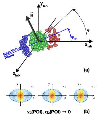
Figure 1: (a) Sketch of a two-nucleus collision in the lab frame, with the left one exiting and the right one entering the page. Particle production occurs in the overlap region. The azimuthal angles of the reaction plane and a produced particle are illustrated. The magnetic field is perpendicular to the reaction plane. (b) Schematic diagram of the event shape selection based on the particle emission pattern in the transverse plane. Both $v_{2}$ and $q_{2}$ for particles of interest could fluctuate towards zero despite a finite eccentricity of the overlap region.

On average, the direction of ${\vec{B}}$ is perpendicular to the reaction plane (${\rm\Psi_{RP}}$), which is defined by impact parameter and beam momenta as illustrated in Fig. 1(a). Consequently, the CME leads to a separation of electric charges normal to the reaction plane. To quantify the CME-induced charge separation and other collectivity modes, we adopt the convention of expressing the azimuthal angle distribution of final-state particles as a Fourier series Sergeiflow1

$$\frac{dN_{\alpha}}{d\varphi}\propto 1+2a_{1,\alpha}\sin\Delta\varphi+\sum_{n=1}^{\infty}2v_{n,\alpha}\cos n\Delta\varphi,$$ (1)

where $\Delta\varphi=\varphi-\Psi_{\rm{RP}}$, $\varphi$ represents the azimuthal angle of a particle’s momentum, and $\alpha$ denotes its charge sign. $a_{1,+}$ and $a_{1,-}$ should bear opposite signs due to the charge separation, and they could have slightly different magnitudes in the presence of extra positive charges in the collision system. The hydrodynamic expansion hydro supposedly transforms the anisotropic initial state in coordinate space into the anisotropy ($v_{n}$) of final-state particles in momentum space. Of all the $v_{n}$ coefficients, the most relevant to the CME search is $v_{2}\equiv\langle\cos 2\Delta\varphi\rangle$, elliptic flow. When averaged over events, $v_{2}$ is roughly proportional to the eccentricity of the initial overlap region. Later, we will explain the relationship between $v_{2}$ and the background in the CME observable, as well as how to suppress such contributions.

A recent study AVFD5 has confirmed the similarity in the core components of the CME observables, such as the $\gamma_{112}$ correlator CME-9 , the $R_{\Psi_{2}}(\Delta S)$ correlator Magdy:2017yje , and the signed balance functions Tang:2019pbl . In this paper, we focus on the most widely used observable CME-9 ,

$$\gamma_{112}\equiv\langle\cos(\varphi_{\alpha}+\varphi_{\beta}-2\Psi_{\rm{RP}})\rangle,$$ (2)

which is averaged over particle pairs and over events. The difference between opposite-sign (OS) and same-sign (SS) pairs contains the true charge separation signal,

$$\Delta\gamma_{112} \equiv \gamma^{\rm{OS}}_{112}-\gamma^{\rm{SS}}_{112}$$ (3)

$$= (a_{1,+}^{2}+a_{1,-}^{2})/2-a_{1,+}a_{1,-}+{\rm BG}$$ (4)

$$= 2a_{1}^{2}+{\rm BG},$$ (5)

where $2a_{1}^{2}\equiv(a_{1,+}^{2}+a_{1,-}^{2})/2-a_{1,+}a_{1,-}$ is shorthand for the CME signal, and BG denotes background contributions to be reckoned with. Experiments at RHIC and the LHC, including STAR STAR-1 ; STAR-2 ; STAR-3 ; LPV_STAR5 ; STAR-4 ; STAR-5 ; STAR-6 ; STAR-7 ; STAR-8 ; STAR-9 , ALICE ALICE-1 ; ALICE-2 ; ALICE-3 , and CMS CMS-1 ; CMS-2 , have reported positively finite $\Delta\gamma_{112}$ measurements for various collision systems and beam energies. However, the data interpretation is hindered by an incomplete understanding of the background. For instance, hitherto, the recent isobar data from STAR STAR-7 cannot yield a definite conclusion on the existence of the CME because of the overwhelming background in addition to the multiplicity mismatch between the two isobaric systems.

The BG term in Eq. (5) consists of both flow and nonflow contributions. Nonflow correlations are unrelated to the reaction plane and originate from various sources such as clusters, resonances, jets, or di-jets. These mechanisms can simultaneously contaminate $\varphi_{\alpha}$, $\varphi_{\beta}$, and the estimation of $\Psi_{\rm RP}$, leading to a finite $\Delta\gamma_{112}$ value even in the absence of genuine $a_{1}$. Nonflow effects are more conspicuous in smaller systems with lower multiplicities, like $p$+Au and $d$+Au collisions at $\sqrt{s_{NN}}=200$ GeV STAR-5 . For the simulation study presented in this work, we will exclusively employ the true reaction plane to avoid nonflow contamination. In practical applications, the reaction plane can be approximated with the event plane defined by spectator nucleons to eliminate nonflow STAR-8 ; STAR-9 . As spectators exit the participant zone early in the collision, the influence of most nonflow mechanisms becomes negligible when the spectator plane is used. While the momentum conservation effect could potentially impact spectators, deploying two spectator planes symmetrically positioned in rapidity effectively eliminates this effect, as demonstrated in prior flow measurements v1_STAR ; v1_ALICE . Even with just one spectator plane, the momentum conservation effect can be nullified in observables like $\Delta\gamma_{112}$, as $\gamma^{\rm{OS}}_{112}$ and $\gamma^{\rm{SS}}_{112}$ are affected in the same manner STAR-3 ; STAR-4 .

The background related to flow can be illustrated through the example of flowing resonances, which undergo decay into particles $\alpha$ and $\beta$ CME-9 :

$${\rm BG}_{\rm res}\propto v_{2}^{\rm res}\langle\cos(\varphi_{\alpha}+\varphi_{\beta}-2\varphi_{\rm res})\rangle.$$ (6)

As an example, consider two $\rho$ mesons traveling in opposite directions, but both within the reaction plane. In this case, $v_{2}^{\rm res}=1$. If the decay pions are so highly boosted as to follow the exact directions of their parents, there exists no out-of-plane charge separation, yet $\Delta\gamma_{112}$ based on these four pions equals 1. The flowing resonance picture can be generalized to a larger portion of, or even the entire, event through the mechanisms of transverse momentum conservation (TMC) Pratt2010 ; Flow_CME and/or local charge conservation (LCC) PrattSorren:2011 ; LCC-1 . Essentially, the flow-related background in $\Delta\gamma_{112}$ can be attributed to the coupling of elliptic flow with other mechanisms, and therefore, should be effectively suppressed by reducing elliptic flow.

The event shape selection (ESS), also called event shape engineering in some literature SergeiESE , classifies collision events according to their shapes and maps the CME observables to a group of events with minimal flow. Ideally, an event shape variable based on final-state particles can accurately reflect the eccentricity of the initial overlap region. The projection to spherical events (zero eccentricity) then guarantees that $v_{2}$ is on average zero for all particles, whether they are primordial particles, resonances, or decay products. However, as demonstrated in Fig. 1(b), the particle emission pattern may exhibit event-by-event fluctuations, resulting in minimal $v_{2}$ measurements despite a finite eccentricity. In reality, it is not a trivial task to devise a feasible and effective ESS procedure.

An early ESS practice categorizes events directly using “observed $v_{2}$” LPV_STAR5 , and faces certain technical challenges in data interpretation 1st-ESS . A more dependable event shape variable is $q_{2}$ Sergeiflow1 ; SergeiESE ; 1st-ESS , the module of the second-order flow vector, $\overrightarrow{q_{2}}=\frac{1}{\sqrt{N}}\bigl{(}\sum_{i=1}^{N}\cos 2\varphi_{i},\sum_{i=1}^{N}\sin 2\varphi_{i}\bigr{)}$. When $q_{2}$ is constructed from a sub-event that does not include particles of interest (POI), the correlation between this $q_{2,{\rm B}}$ and $v_{2,{\rm POI}}$ is typically weak, and even at zero $q_{2,{\rm B}}$, $v_{2,{\rm POI}}$ is still positive and sizable. As a result, the extrapolation of $\Delta\gamma_{112}$ over a wide, unmeasured $v_{2,{\rm POI}}$ region introduces substantial statistical and systematic uncertainties ALICE-2 ; CMS-2 . We have also demonstrated this point in Appendix A. To circumvent lengthy extrapolations in $v_{2}^{\rm POI}$, we adopt the approach outlined in Ref. 1st-ESS that builds $q_{2}$ upon POI, $q_{2,{\rm POI}}$. For simplicity, we will use $q_{2}$ to represent $q_{2,{\rm POI}}$ throughout the paper, except in Appendix A. Besides the technical justification, potential longitudinal flow-plane decorrelations torque ; HydroFluc ; Glasma ; Dynamic ; EccenDecorr highlight the importance of maintaining POI and $q_{2}$ within the same rapidity region. Furthermore, we will incorporate information on particle pairs and expand the ESS method into four variants.

In Sec. II we will describe the ESS methodology in detail. Sec. III briefly outlines the models to be used in the upcoming simulation studies, including a toy model toymodel and the event-by-event anomalous-viscous fluid dynamics (EBE-AVFD) model AVFD1 ; AVFD2 ; AVFD4 . In Sec. IV, we investigate the relationship between resonance $v_{2}$ and both the background and, remarkably, the CME signal. We also perform a quantitative assessment of the efficacy of the ESS variants in mitigating the background for $\Delta\gamma_{112}$. In Sec. V we provide a summary and offer an outlook.

II Event Shape Selection

Prior studies 1st-ESS have demonstrated that, compared with $q_{2}$, $q_{2}^{2}$ renders a more reliable projection of $\Delta\gamma_{112}$ to the zero-flow limit. Based on the expansion,

$$q^{2}_{2} = \frac{1}{N}\biggl{[}\biggl{(}\sum^{N}_{i=1}\sin 2\varphi_{i}\biggr{)}^{2}+\biggl{(}\sum^{N}_{i=1}\cos 2\varphi_{i}\biggr{)}^{2}\biggr{]}$$ (7)

$$= 1+\frac{1}{N}\sum_{i\neq j}\cos[2(\varphi_{i}-\varphi_{j})],$$

we estimate the event average of $q_{2}^{2}$,

$$\langle q_{2}^{2}\rangle\approx 1+Nv_{2}^{2}\{2\}.$$ (8)

Here, $v_{2}\{2\}$ is the ensemble average of elliptic flow obtained from two-particle correlations. Eqs. (7) and (8) reveal the link between the event shape variable and the elliptic flow variable, and warrants a correction to the normalization for $q_{2}$. Hereafter, we redefine $q_{2}^{2}$ as

$$q^{2}_{2}=\frac{\bigl{(}\sum^{N}_{i=1}\sin 2\varphi_{i}\bigr{)}^{2}+\bigl{(}\sum^{N}_{i=1}\cos 2\varphi_{i}\bigr{)}^{2}}{N(1+Nv_{2}^{2}\{2\})}.$$ (9)

Note that $N$ varies from event to event, whereas $v_{2}\{2\}$ is a static constant averaged over all events. The correction due to the new term in the normalization becomes prominent when $N$ is large.

As mentioned in Sec. I, we construct $q_{2}$ upon POI, in hope that the $q_{2}$ and $v_{2}$ based on single particles largely reflect the initial geometry of the collision system. However, the anisotropy of particle pairs could be more pertinent to the background contribution in $\gamma_{112}$ which correlates the reaction plane with a pair of particles, instead of single particles. For instance, to the background arising from flowing resonances, the $v_{2}$ and the corresponding $q_{2}$ of the parent resonances should be more relevant than those of the kindred decay daughters. More generally, the background caused by LCC entails primordial particles that contribute as if they had hypothetical flowing progenitors. Accordingly, we invoke the pair azimuthal angle, $\varphi^{\rm p}$, from the momentum sum for each pair of POI, regardless of the existence of a genuine parent. The corresponding elliptic flow variable (pair $v_{2}$) and event shape variable (pair $q^{2}_{2}$) are expressed as

$$v_{2,\rm{pair}} = \langle\cos(2\varphi^{\rm p}-2\Psi_{\rm{RP}})\rangle,$$ (10)

$$q^{2}_{2,{\rm pair}} = \frac{\bigl{(}\sum^{N_{\rm pair}}_{i=1}\sin 2\varphi_{i}^{\rm p}\bigr{)}^{2}+\bigl{(}\sum^{N_{\rm pair}}_{i=1}\cos 2\varphi_{i}^{\rm p}\bigr{)}^{2}}{N_{\rm pair}(1+N_{\rm pair}v_{2,{\rm pair}}^{2}\{2\})},$$ (11)

respectively. In Eq. (11), the correction term in the normalization is crucial, given that $N_{\rm pair}$ is basically on the order of $N^{2}/2$.

Our ESS analysis closely follows the procedure described in Ref. ESS-1 . Firstly, we group events according to the event shape variable and compute both $\Delta\gamma_{112}$ and the elliptic flow variable for each group. Next, we study the dependence of $\Delta\gamma_{112}$ on the elliptic flow variable and project it to the zero-flow limit. Now that both the event shape variable and the elliptic flow variable can be calculated either from single particles or from particle pairs, we will discuss the following four combinations.

Since the unmixed recipes (with single $q_{2}^{2}$ and single $v_{2}$ or with pair $q_{2}^{2}$ and pair $v_{2}$) rely on the azimuthal angles of the same POI or the same pairs, there could be intrinsic correlations between the event shape variable and the elliptic flow variable, as indicated by Eqs. (7) and (8). Therefore, the projection to the zero-flow limit may be prone to bias, causing a residual background. Conversely, the mixed recipes (with single $q_{2}^{2}$ and pair $v_{2}$ or with pair $q_{2}^{2}$ and single $v_{2}$) enhance the mutual independence between the event shape variable and the elliptic flow variable, and could improve the extrapolation. The sensitivity of all four approaches to background subtraction will be tested in the forthcoming sections.

III Model Descriptions

The simple toy model toymodel without the CME aims to investigate the background mechanism due to flowing resonances. In each event, we generate 33 pairs of $\pi^{\pm}$ that come from $\rho$ meson decays, the multiplicity of which roughly matches the STAR measurements within the rapidity range of $|y|<1$ in 30–40% Au+Au collisions at $\sqrt{s_{NN}}$ = 200 GeV mult_200 ; percent_17 . The inputs of spectrum and elliptic flow for $\rho$ mesons follow the same procedure as adopted in Ref. toymodel . The decay process, $\rho\rightarrow\pi^{+}+\pi^{-}$, is implemented with PYTHIA6 pythia6 . In this study, we only select pions within $0.2<p_{T}<2$ GeV/$c$.

The EBE-AVFD model AVFD1 ; AVFD2 ; AVFD4 incorporates the dynamical CME transport for light quarks, and effectively handles the background mechanisms like flowing resonances, TMC, and LCC. The initial conditions for entropy density ($s$) profiles and for electromagnetic field follow the event-by-event nucleon configuration from the Monte Carlo Glauber simulations glauber . The input of chirality charge density ($n_{5}$) takes the form of $n_{5}/s$. The CME transport is governed by anomalous hydrodynamic equations as a linear perturbation on top of the medium flow that is managed by the VISH2+1 simulation package AVFD3 . In the freeze-out process, the LCC effect is specifically tuned to match experimental data. After being produced from the freeze-out hypersurface, all hadrons undergo hadron cascades using the UrQMD simulations Bleicher:1999xi , which account for various resonance decay processes and automatically factor in their contributions to the charge-dependent correlations. We focus on the 30–40% centrality range of Au+Au collisions at $\sqrt{s_{NN}}=200$ GeV, using the same settings and input parameters as adopted in Ref. AVFD5 . The numbers of events are $9.6\times 10^{7}$, $5.9\times 10^{7}$, and $7.7\times 10^{7}$ for the cases of $n_{5}/s=0$, 0.1, and 0.2, respectively. For simplicity, the analysis uses the true reaction plane. The POI are $\pi^{\pm}$ within $|y|<1$ and $0.2<p_{T}<2$ GeV/$c$.

IV simulation results

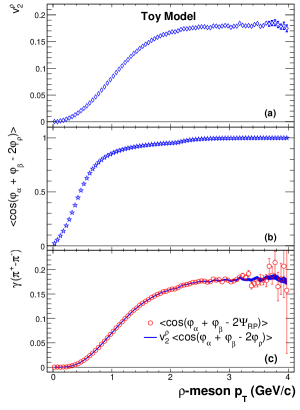
Figure 2: Toy model simulations of (a) $\rho$-meson $v_{2}$, (b) the correlation between a $\rho$ meson and its daughter pions, $\langle\cos(\varphi_{\alpha}+\varphi_{\beta}-2\varphi_{\rho})\rangle$, and (c) the $\gamma_{112}$ correlator between two sibling pions, as a function of $\rho$-meson $p_{T}$. For comparison, the product, $v_{2}^{\rho}\langle\cos(\varphi_{\alpha}+\varphi_{\beta}-2\varphi_{\rho})\rangle$, is shown with a shaded band.

Figure 2(a) shows the input of $\rho$-meson $v_{2}$ for the toy model, and Fig. 2(b) presents the correlation between a $\rho$ meson and its daughter pions, $\langle\cos(\varphi_{\alpha}+\varphi_{\beta}-2\varphi_{\rho})\rangle$, which is solely due to decay kinematics. As $\rho$-meson $p_{T}$ increases, the two daughters display enhanced collimation towards the direction of the parent’s motion. Figure 2(c) shows the resultant $\gamma_{112}$ correlator between two sibling pions, which agrees very well with the product, $v_{2}^{\rho}\langle\cos(\varphi_{\alpha}+\varphi_{\beta}-2\varphi_{\rho})\rangle$. This agreement corroborates the relation stated in Eq. (6) and confirms the background mechanism due to the decay of flowing resonances.

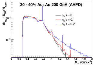
Figure 3: EBE-AVFD calculations of the per-event-normalized excess of opposite-sign $\pi$-$\pi$ pairs over same-sign ones vs invariant mass in 30–40% Au+Au collisions at 200 GeV. In the low-mass region, the results from top to bottom correspond to the cases of $n_{5}/s=$ 0, 0.1, and 0.2, respectively. The ordering is inverted in the high-mass region. The sharp peaks resemble resonances such as $\rho$ meson.

Given the consistently positive nature of $\langle\cos(\varphi_{\alpha}+\varphi_{\beta}-2\varphi_{\rho})\rangle$ without any sign change, it is tempting to directly use resonance $v_{2}$ as the elliptic flow variable for background control. However, we realize that the experimental manifestation of resonances, the excess of OS over SS particle pairs, is affected by the CME. Figure 3 delineates the EBE-AVFD simulations of the per-event-normalized invariant mass distribution for the excess of OS over SS pion pairs in 30–40% Au+Au collisions at 200 GeV. The invariant mass of two pions is intimately linked to the opening angle between them. The presence of the CME, characterized by finite $n_{5}/s$ values, tends to induce an opposing motion of $\pi^{+}$ and $\pi^{-}$, enhancing the observed resonance yield at higher invariant mass, and meanwhile depleting the lower-mass region.

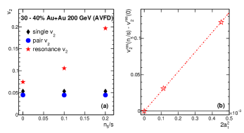
Figure 4: (a) EBE-AVFD simulations of single $v_{2}$, pair $v_{2}$, and resonance $v_{2}$ as a function of $n_{5}/s$ in 30–40% Au+Au collisions at 200 GeV. (b) Background subtracted resonance $v_{2}$ vs $2a_{1}^{2}$. The linear fit passing through $(0,0)$ demonstrates that resonance $v_{2}$ contains the CME signal proportional to $a_{1}^{2}$.

The CME not only impacts the invariant mass spectrum of observed resonances, but also modifies the corresponding $v_{2}$ observable,

$$v_{2}^{\rm res}\equiv\frac{N_{\rm{OS}}\langle\cos 2\Delta\varphi^{\rm{OS}}\rangle-N_{\rm{SS}}\langle\cos 2\Delta\varphi^{\rm{SS}}\rangle}{N_{\rm{OS}}-N_{\rm{SS}}},$$ (12)

where $\Delta\varphi^{\rm{OS(SS)}}$ denotes the azimuthal angle of an OS(SS) particle pair with respect to $\Psi_{\rm RP}$. Figure 4(a) shows the EBE-AVFD calculations of single $v_{2}$, pair $v_{2}$, and resonance $v_{2}$ as a function of $n_{5}/s$. The former two essentially remain the same, whereas resonance $v_{2}$ linearly increases with the strength of the CME. Here, we take the entire invariant mass range without selecting any specific resonance. Figure 4(b) presents the background subtracted resonance $v_{2}$ vs $2a_{1}^{2}$. We apply a linear fit passing through $(0,0)$ to demonstrate that resonance $v_{2}$ contains the CME signal proportional to $a_{1}^{2}$.

As derived analytically in Appendix B with certain simplifications, resonance $v_{2}$ is another CME observable,

$$v_{2}^{\rm res} \approx v_{2}^{\pi}+\frac{N_{\rm{OS}}+N_{\rm{SS}}}{2(N_{\rm{OS}}-N_{\rm{SS}})}(\Delta\gamma_{112}-v_{2}^{\pi}\Delta\delta)$$ (13)

$$+\frac{1}{2}(\gamma^{\rm OS}+\gamma^{\rm SS})-\frac{v_{2}^{\pi}}{2}(\delta^{\rm OS}+\delta^{\rm SS}),$$

where $\delta\equiv\langle\cos(\varphi_{\alpha}-\varphi_{\beta})\rangle$ is the two-particle correlation. Since $(N_{\rm{OS}}+N_{\rm SS})/(N_{\rm{OS}}-N_{\rm{SS}})$ is typically on the order of a few hundred, the second term in Eq. (13) is comparable to $v_{2}^{\pi}$. This makes resonance $v_{2}$ unsuitable as an elliptic flow variable in the ESS method. Figure 5 shows the EBE-AVFD simulations of $\pi$-$\pi$ $\Delta\gamma_{112}$ as a function of $v_{2}^{\rm res}$ categorized by single $q_{2}^{2}$ in the scenarios of $n_{5}/s=0$ (a) and 0.1 (b). The $y$-intercepts obtained with linear fits reveal the over-subtraction of background, especially pronounced when the true CME signal, $2a_{1}^{2}$, is finite.

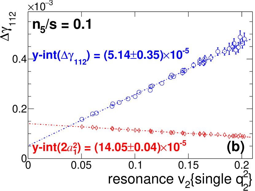
Figure 5: EBE-AVFD simulations of $\Delta\gamma_{112}$ as a function of resonance $v_{2}$ categorized by single $q_{2}^{2}$ in the scenarios of $n_{5}/s=0$ (a) and 0.1 (b) in 30–40% Au+Au collisions at 200 GeV. The particles of interest are charged pions. For comparison, $2a_{1}^{2}$ is also added in panel (b). The $y$-intercepts obtained with linear fits demonstrate the over-subtraction of the elliptic-flow-related background.

Similarly, pair $v_{2}$ also contains the CME signal:

$$v_{2,{\rm pair}} = \frac{N_{\rm{OS}}\langle\cos 2\Delta\varphi^{\rm{OS}}\rangle+N_{\rm{SS}}\langle\cos 2\Delta\varphi^{\rm{SS}}\rangle}{N_{\rm{OS}}+N_{\rm{SS}}}$$ (15)

$$\approx v_{2}^{\pi}+\frac{N_{\rm{OS}}-N_{\rm{SS}}}{2(N_{\rm{OS}}+N_{\rm{SS}})}(\Delta\gamma_{112}-v_{2}^{\pi}\Delta\delta)$$

$$+\frac{1}{2}(\gamma^{\rm OS}+\gamma^{\rm SS})-\frac{v_{2}^{\pi}}{2}(\delta^{\rm OS}+\delta^{\rm SS}).$$

Considering the small values of $(N_{\rm OS}-N_{\rm{SS}})/(N_{\rm{OS}}+N_{\rm{SS}})$ and later terms, pair $v_{2}$ is evidently dominated by $v_{2}^{\pi}$, leading to the observed constancy of pair $v_{2}$ in Fig. 4(a). However, when using pair $v_{2}$ as the elliptic flow variable for background control, the second term in Eq. (15) becomes nonnegligible, because the over-subtraction of background as demonstrated in Fig. 5 is still present, although to a lesser extent.

Previous works using EBE-AVFD ESS-1 have shown that constructing both $v_{2}$ and $q_{2}$ from the same group of particles can introduce inherent self-correlations. Consequently, the unmixed ESS variants (with single $q_{2}^{2}$ and single $v_{2}$ or with pair $q_{2}^{2}$ and pair $v_{2}$) tend to under-subtract the background. To mitigate such residual backgrounds, we have introduced in Sec. II mixed combinations (with pair $q_{2}^{2}$ and single $v_{2}$ or with single $q_{2}^{2}$ and pair $v_{2}$). However, as mentioned in the preceding paragraph, pair $v_{2}$ also encompasses the CME signal, which could cause an over-subtraction of background in $\Delta\gamma_{112}$. Therefore, the ESS recipe using single $v_{2}$ as the elliptic flow variable and pair $q_{2}^{2}$ as the event shape variable emerges as the optimal solution.

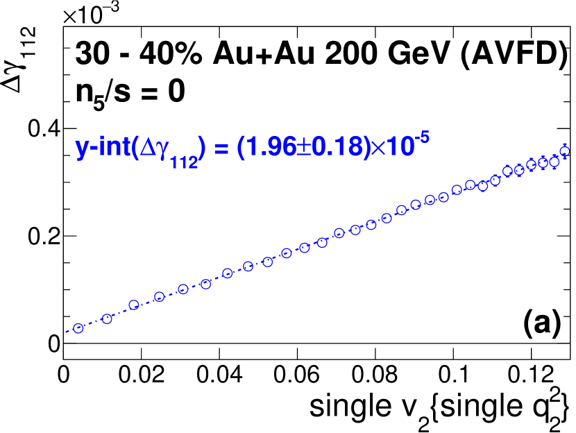
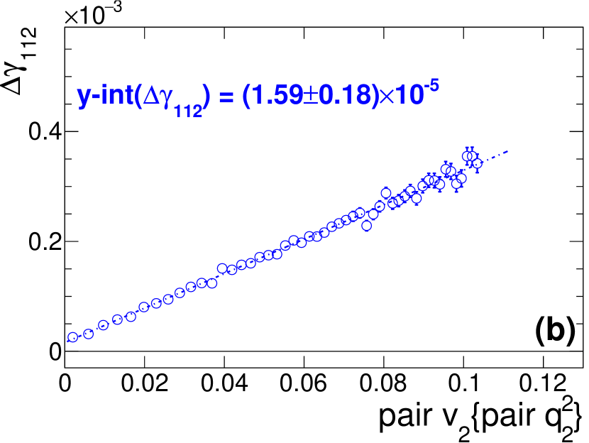
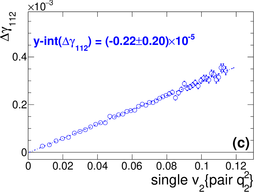
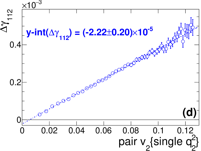
Figure 6: EBE-AVFD simulations of $\Delta\gamma_{112}$ as a function of single or pair $v_{2}$ categorized by single or pair $q_{2}^{2}$ in the pure background scenario ($n_{5}/s=0$) in 30–40% Au+Au collisions at 200 GeV. The particles of interest are charged pions. The $y$-intercepts obtained with linear fits reflect the efficacy of these ESS recipes in reducing the elliptic-flow-related background.

Figure 6 shows the EBE-AVFD simulations of the $\pi$-$\pi$ $\Delta\gamma_{112}$ correlation as a function of $v_{2}$ categorized by $q_{2}^{2}$ in the pure background scenario ($n_{5}/s=0$) in 30–40% Au+Au collisions at 200 GeV. Since both $v_{2}$ and $q_{2}^{2}$ can be computed from either single particles or particle pairs, we present each of the four cases in a separate panel. The $y$-intercepts obtained from single $v_{2}${single $q_{2}^{2}$} and pair $v_{2}${pair $q_{2}^{2}$} reflect an approximate eight-fold suppression of background, but they remain finite, indicative of residual backgrounds. The ESS result using single $v_{2}${pair $q_{2}^{2}$} is consistent with zero, whereas the one using pair $v_{2}${single $q_{2}^{2}$} appears to over-subtract the background, as expected.

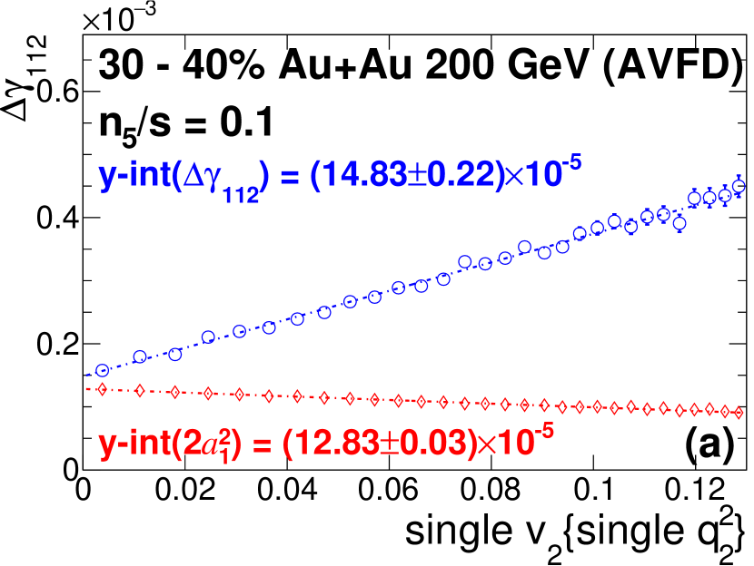
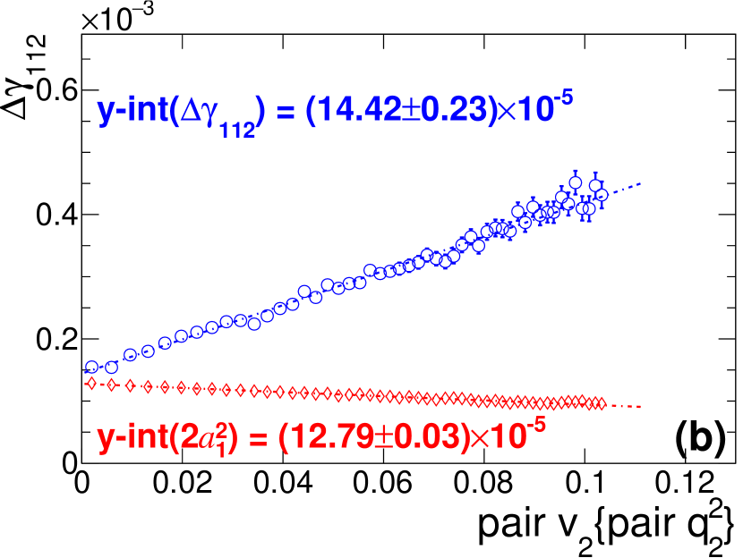
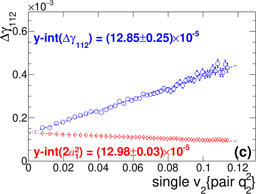
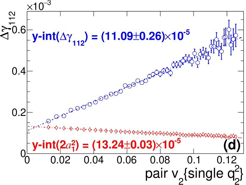
Figure 7: EBE-AVFD simulations of $\Delta\gamma_{112}$ (blue circle) and $2a_{1}^{2}$ (red diamond) as a function of single or pair $v_{2}$ categorized by single or pair $q_{2}^{2}$ in the moderate CME scenario ($n_{5}/s=0.1$) in 30–40% Au+Au collisions at 200 GeV. The particles of interest are charged pions. The $y$-intercepts obtained with linear fits reflect the efficacy of these ESS recipes in revealing the true CME signal.

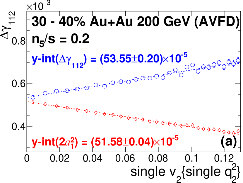
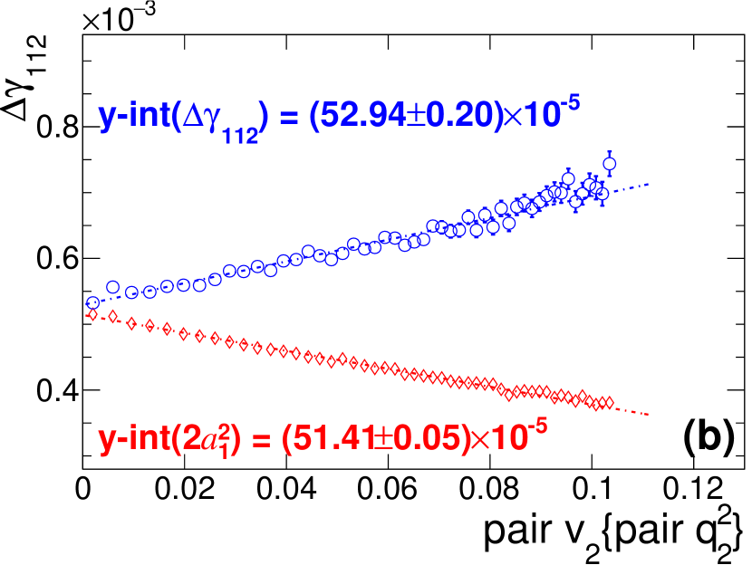
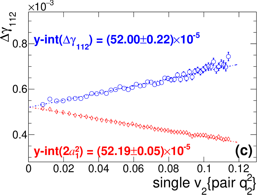
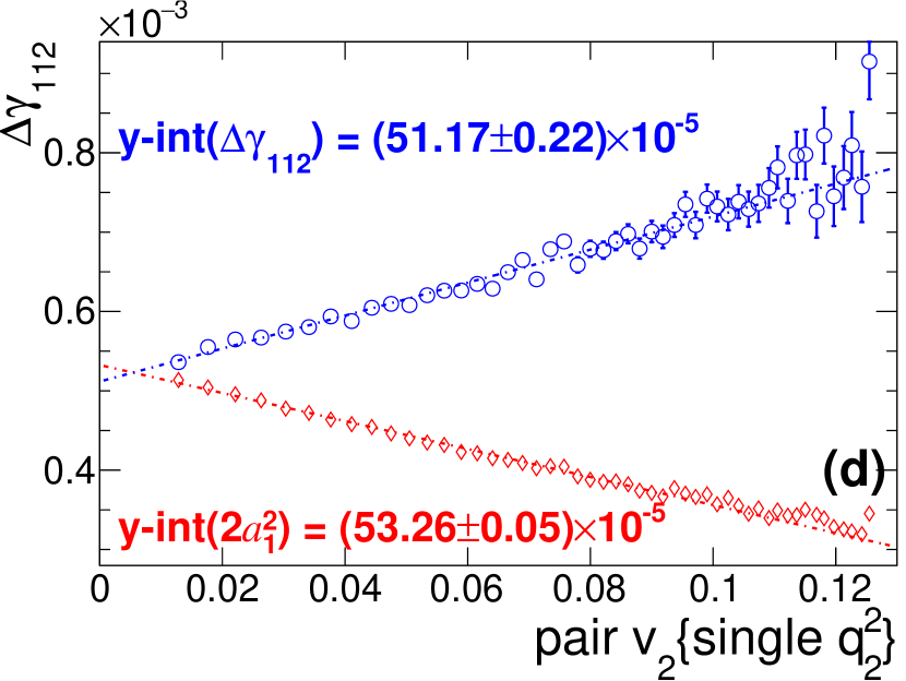
Figure 8: The same as in Fig. 7, but for the strong CME scenario ($n_{5}/s=0.2$).

Figures 7 and 8 depict scenarios that are analogous to Fig. 6, but for moderate and strong CME signals with $n_{5}/s=0.1$ and 0.2, respectively. For comparison, we also project the true CME signal, $2a_{1}^{2}$, to zero $v_{2}$. In both scenarios, the $y$-intercepts of $\Delta\gamma_{112}$ obtained from single $v_{2}${single $q_{2}^{2}$} and pair $v_{2}${pair $q_{2}^{2}$} are significantly above the actual signal, while that using pair $v_{2}${single $q_{2}^{2}$} overestimates the background. The analyses using single $v_{2}${pair $q_{2}^{2}$} seem to recover the true signal within the uncertainties. Therefore, the ESS outcomes are most reliable when we use pair $q_{2}^{2}$ for event shape selection and single-particle $v_{2}$ for background control.

As portrayed in Figs. 7 and 8, $a_{1}^{2}$ itself increases during the ESS extrapolation to the zero-flow limit. To restore the ensemble average of the CME signal, we need to scale the $y$-intercept of $\Delta\gamma_{112}$ with an appropriate factor. Recent research, based on the concept of noninterdependent processes asynchronous , suggests that the observed $a_{1}$ intrinsically decreases as $v_{2}$ increases, implying that $\langle a_{1}\rangle=a_{1}|_{v_{2}=0}\cdot(1-\langle v_{2}\rangle)$. Here, $v_{2}$ represents single-particle $v_{2}$, typically on the order of 5%. Moreover, higher-order effects could exist even without considering the noninterdependent effect 1st-ESS . Hence, to reestablish the CME signal for the inclusive data, we need to multiply the $y$-intercept of $\Delta\gamma_{112}$ by a factor of $(1-\langle v_{2}\rangle)^{2}$, to the first order.

In the past, various event generators have been employed to investigate the background contributions to the $\gamma_{112}$ correlator. Notably, models like PYTHIA pythia , HIJING hijing1 ; hijing2 , MEVSIM mevsim , and UrQMD urqmd substantially underestimate the background STAR-2 ; STAR-4 . While the AMPT model ampt_1 ; ampt_5 is able to reproduce some background contributions comparable to experimental measurements Subikash , even a straightforward ESS application using single $v_{2}$ and single $q_{2}^{2}$ can effectively eliminate all the AMPT-generated backgrounds ESS-1 . The outcomes of our four ESS recipes from the AMPT simulations (not shown here) exhibit the same ordering as observed in EBE-AVFD, with the tendency to over-subtract the background. EBE-AVFD is hitherto the most realistic model for the CME simulations and the only one that necessitates a mixed combination of $v_{2}$ and $q_{2}^{2}$ to completely remove the backgrounds in $\Delta\gamma_{112}$. We have also explored augmenting the strength of the LCC effect by half in the EBE-AVFD simulations and confirmed that the conclusions drawn from Figs. 6, 7, and 8 remain unchanged. The ultimate validation of the new method hinges on its application to real data, such as Au+Au collisions at 3 GeV, where the QGP (along with the CME) is expected to be absent 3GeV ; 3GeV_2 ; 3GeV_3 .

V Conclucsion

The experimental search for the CME in heavy-ion collisions remains a challenging task because of the flow related background in the observables. In this work, we propose an innovative ESS scheme based on a previous work ESS-1 so as to effectively suppress the non-CME background and accurately extract the CME signal under various experimental scenarios. Our comprehension of background suppression has been advanced in several aspects. First, we improve the definition of the flow vector by correcting the normalization with a higher-order term. This refinement ensures a more reliable ESS projection, especially for events with high multiplicities.

Second, we extensively investigate one of the primary background sources, flowing resonances. With the help of a toy model, we validate that in the absence of the CME, this background arises from the product of resonance $v_{2}$ and the correlation between the resonance and its decay daughters. Moreover, we analytically deduce that resonance $v_{2}$ incorporates the CME signal, which is further supported by EBE-AVFD simulations. Thus, the utilization of resonance $v_{2}$ as an elliptic flow variable in the ESS approach is not recommended, as it leads to a severe over-subtraction of background. Similarly, according to a recent study spin_alignment , the spin alignment ($\rho_{00}$) of resonances should not be considered solely as a background contribution but rather as another CME observable. Extra caution is necessary when developing methods for background control using variables such as resonance $v_{2}$, $\rho_{00}$, or even invariant mass.

Third, by incorporating particle pair information, we expand the ESS technique to include four distinct combinations of event shape and elliptic flow variables. The unmixed recipes exploit the azimuthal angles of either the same POI or the same pairs to construct both the event shape variable and the elliptic flow variable, generating intrinsic correlations that lead to an under-subtraction of background. Conversely, the mixed recipe using pair $v_{2}$ as the elliptic flow variable (and single $q_{2}^{2}$ as the event shape variable) over-subtracts the background, because pair $v_{2}$ contains the CME signal, albeit in a diluted form. Therefore, the optimal event shape selection strategy involves utilizing single $v_{2}$ in conjunction with pair $q_{2}^{2}$. These findings have been supported by EBE-AVFD calculations. Additionally, in Appendix A, we have demonstrated that using an event shape variable devoid of POI yields much larger uncertainties, both statistically and systematically.

In short, we have pinpointed a technically robust ESS approach, which effectively mitigates the flow-related background in the $\Delta\gamma_{112}$ correlator. We eagerly anticipate the application of the method outlined in this paper to real-data analyses in the pursuit of the CME in the heavy-ion collisions.

Appendix A Event shape variable exclusive of POI

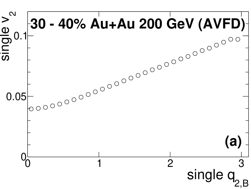
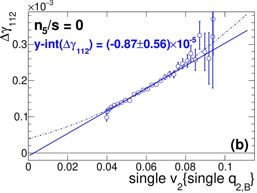
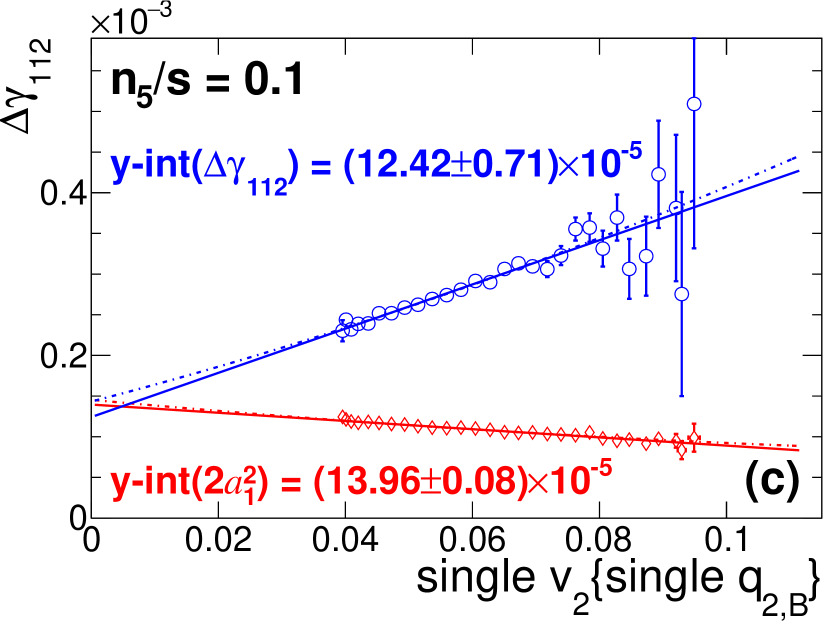
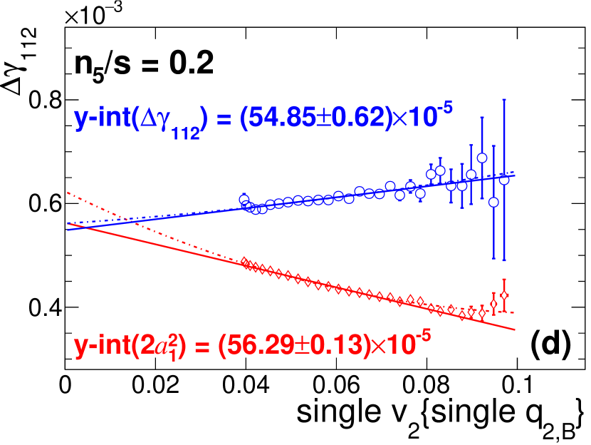
Figure 9: EBE-AVFD simulations of single $v_{2}$ as a function of single $q_{2,{\rm B}}$ (a) and $\Delta\gamma_{112}$ as a function of single $v_{2}$ categorized by single $q_{2,{\rm B}}$ in the scenarios of $n_{5}/s=0$ (b), 0.1 (c), and 0.2 (d) in 30–40% Au+Au collisions at 200 GeV. The particles of interest are charged pions. The $y$-intercepts obtained with linear fits (solid lines) reflect the efficacy of these ESS recipes in reducing the elliptic-flow-related background. The second-order polynomial fits (dashes lines) demonstrate the systematic uncertainties due to long extrapolations.

To examine the event shape variable exclusive of POI, we construct $q_{2,{\rm B}}$ as defined in Eq. (9) using single particles with $1<|y|<2$, while POI are within $|y|<1$. Figure 9(a) shows the EBE-AVFD simulations of single $v_{2}$ as a function of single $q_{2,{\rm B}}$ in 30–40% Au+Au collisions at 200 GeV. Compared with the $q_{2}^{2}$ involving POI, $q_{2,{\rm B}}$ exhibits a weaker correlation with single $v_{2}$, and the latter remains sizable at zero $q_{2,{\rm B}}$. Figures 9(b)–9(d) present $\Delta\gamma_{112}$ as a function of single $v_{2}$ categorized by single $q_{2,{\rm B}}$ in the scenarios of $n_{5}/s=0$, 0.1, and 0.2, respectively. The $y$-intercepts obtained with linear fits (solid lines) indicate a certain degree of over-subtraction of background. The extensive blank regions at low $v_{2}$ considerably amplifies the statistical uncertainties of the $y$-intercepts, leading to an approximate tripling of the uncertainties compared with using event shape variables involving POI. Moreover, if we alternatively apply second-order polynomial fits (dashes lines), the variations of the $y$-intercepts could exceed the statistical uncertainties, exacerbating the issue further. Conversely, employing POI for the event shape variable renders significantly more reliable results, in terms of both statistical accuracy and systematic consistency.

Appendix B Resonance $v_{2}$

For simplicity, we set $\Psi_{\rm RP}=0$, and assume that particles $\alpha$ and $\beta$ have the same $p_{T}$. We thus obtain $\tan\varphi^{\rm p}=(\sin\varphi_{\alpha}+\sin\varphi_{\beta})/(\cos\varphi_{\alpha}+\cos\varphi_{\beta})$, where $\varphi^{\rm p}$ is the azimuthal angle of this particle pair. Then, the following trigonometric identity becomes

$$\cos 2\varphi^{\rm p} = (1-\tan^{2}\varphi^{\rm p})/(1+\tan^{2}\varphi^{\rm p})$$ (16)

$$= \frac{\cos 2\varphi_{\alpha}+\cos 2\varphi_{\beta}+2\cos(\varphi_{\alpha}+\varphi_{\beta})}{2+2\cos(\varphi_{\alpha}-\varphi_{\beta})}.$$

Averaging Eq. (16) over OS or SS pairs and over events, we have

$$\langle\cos 2\varphi^{\rm OS(SS)}\rangle \approx (v_{2}^{\pi}+\gamma^{\rm OS(SS)})/(1+\delta^{\rm OS(SS)})$$ (17)

$$\approx v_{2}^{\pi}+\gamma^{\rm OS(SS)}-v_{2}^{\pi}\delta^{\rm OS(SS)},$$

where $\delta\equiv\langle\cos(\varphi_{\alpha}-\varphi_{\beta})\rangle$ is the two-particle correlation. We have assumed $|\delta|\ll 1$ and ignored higher-order terms. Resonance $v_{2}$ is the elliptic flow for the excess of OS over SS pairs,

$$v_{2}^{\rm res} = \frac{N_{\rm{OS}}\langle\cos 2\varphi^{\rm{OS}}\rangle-N_{\rm{SS}}\langle\cos 2\varphi^{\rm{SS}}\rangle}{N_{\rm{OS}}-N_{\rm{SS}}}$$ (19)

$$\approx v_{2}^{\pi}+\frac{N_{\rm{OS}}+N_{\rm{SS}}}{2(N_{\rm{OS}}-N_{\rm{SS}})}(\Delta\gamma_{112}-v_{2}^{\pi}\Delta\delta)$$

$$+\frac{1}{2}(\gamma^{\rm OS}+\gamma^{\rm SS})-\frac{v_{2}^{\pi}}{2}(\delta^{\rm OS}+\delta^{\rm SS}),$$

where $\Delta\delta=\delta^{\rm{OS}}-\delta^{\rm{SS}}$. Regarding the connection to the CME signal, resonance $v_{2}$ is notably similar to the signed balance functions AVFD5 .

References

- (1) D. Kharzeev, Phys. Lett. B 633, 260 (2006).
- (2) D. Kharzeev and A. Zhitnitsky, Nucl. Phys. A 797, 67 (2007).
- (3) D. E. Kharzeev, L. D. McLerran, and H. J. Warringa, Nucl. Phys. A 803, 227 (2008).
- (4) K. Fukushima, D. E. Kharzeev, and H. J. Warringa, Phys. Rev. D 78, 074033 (2008).
- (5) D. Kharzeev, R. D. Pisarski, and M. H. G. Tytgat, Phys. Rev. Lett. 81, 512 (1998).
- (6) D. Kharzeev and R. D. Pisarski, Phys. Rev. D 61, 111901(R) (2000).
- (7) D. E. Kharzeev, Annu. Rev. Nucl. Part. Sci. 65, 193 (2015).
- (8) V. Skokov, A. Illarionov, and V. Toneev, Int. J. Mod. Phys. A 24, 5925 (2009).
- (9) W.-T. Deng and X.-G. Huang, Phys. Rev. C 85, 044907 (2012).
- (10) A. M. Poskanzer, S. A. Voloshin Phys. Rev. C 58, 1671 (1998).
- (11) U. Heinz and R. Snellings, Ann. Rev. Nucl. Part. Sci. 63, 123 (2013).
- (12) S. Choudhury et al., Chin. Phys. C 46, 014101 (2022).
- (13) S. A. Voloshin, Phys. Rev. C 70, 057901 (2004).
- (14) N. Magdy, S. Shi, J. Liao, N. Ajitanand, R. A. Lacey, Phys. Rev. C 97, 061901 (2018).
- (15) A. H. Tang, Chin. Phys. C 44, 054101 (2020).
- (16) B. I. Abelev et al. [STAR Collaboration], Phys. Rev. Lett. 103, 251601 (2009).
- (17) B. I. Abelev et al. [STAR Collaboration], Phys. Rev. C 81, 054908 (2010).
- (18) L. Adamczyk et al. [STAR Collaboration], Phys. Rev. C 88, 064911 (2013).
- (19) L. Adamczyk et al. [STAR Collaboration], Phys. Rev. C 89, 044908 (2014).
- (20) L. Adamczyk et al. [STAR Collaboration], Phys. Rev. Lett. 113, 052302 (2014).
- (21) J. Adam et al. [STAR Collaboration], Phys. Lett. B 798, 134975 (2019).
- (22) M. S. Abdallah et al. [STAR Collaboration], Phys. Rev. C 106, 034908 (2022).
- (23) M. S. Abdallah et al. [STAR Collaboration], Phys. Rev. C 105, 014901 (2022).
- (24) M. S. Abdallah et al. [STAR Collaboration], Phys. Rev. Lett. 128, 092301 (2022).
- (25) B. E. Aboona et al. [STAR Collaboration], Phys. Lett. B 839, 137779 (2023).
- (26) B. Abelev et al. [ALICE Collaboration], Phys. Rev. Lett. 110, 012301 (2013).
- (27) S. Acharya et al. [ALICE Collaboration], Phys. Lett. B 777, 151 (2018).
- (28) S. Acharya et al. [ALICE Collaboration], J. High Energy Phys. 09, 160 (2020).
- (29) V. Khachatryan et al. [CMS Collaboration], Phys. Rev. Lett. 118, 122301 (2017).
- (30) A. M. Sirunyan et al. [CMS Collaboration], Phys. Rev. C 97, 044912 (2018).
- (31) J. Adams et al. [STAR Collaboration], Phys. Rev. C 73, 34903 (2006).
- (32) B. Abelev et al. [ALICE Collaboration], Phys. Rev. Lett. 111, 232302 (2013).
- (33) S. Pratt, S. Schlichting and S. Gavin, Phys. Rev. C 84, 024909 (2011).
- (34) A. Bzdak, V. Koch and J. Liao, Lect. Notes Phys. 871, 503 (2013).
- (35) S. Schlichting and S. Pratt, Phys. Rev. C 83, 014913 (2011).
- (36) W.-Y. Wu et al., Phys. Rev. C 107, L031902 (2023).
- (37) J. Schukraft, A. Timmins, S. A. Voloshin, Phys. Lett. B 719, 394 (2013).
- (38) F. Wen, J. Bryon, L. Wen, G. Wang, Chin. Phys. C 42, 014001 (2018).
- (39) P. Bozek, W. Broniowski, and J. Moreira, Phys. Rev. C 83, 034911 (2011).
- (40) L.-G. Pang, G.-Y. Qin, V. Roy, X.-N. Wang, and G.-L. Ma, Phys. Rev. C 91, 044904 (2015).
- (41) B. Schenke and S. Schlichting, Phys. Rev. C 94, 044907 (2016).
- (42) Shen, Chun and Schenke, Bjorn, Phys. Rev. C 97, 024907 (2018).
- (43) A. Behera, M. Nie, and J. Jia, (2020), Phys. Rev. Res. 2, 023362 (2020).
- (44) A. H. Tang, Chin. Phys. C 44, 054101 (2020).
- (45) S. Shi, Y. Jiang, E. Lilleskov, J. Liao, Ann. Phys. 394, 50 (2018).
- (46) Y. Jiang, S. Shi, Y. Yin and J. Liao, Chin. Phys. C 42, no. 1, 011001 (2018).
- (47) S. Shi, H. Zhang, D. Hou and J. Liao, Phys. Rev. Lett. 125, 242301 (2020).
- (48) R. Milton, G. Wang, M. Sergeeva, S. Shi, J. Liao, and H. Huang. Rev. C 104, 064906 (2021).
- (49) B. I. Abelev et al. [STAR Collaboration], Phys. Rev. C 79, 034909 (2009).
- (50) J. Adams et al. [STAR Collaboration], Phys. Rev. Lett. 92, 092301 (2004).
- (51) T. Sjostrand, S. Mrenna and P. Z. Skands, JHEP 0605, 026 (2006).
- (52) B.B. Back et al., Phys. Rev. C 65, 031901(R) (2002); K. Adcox et al., Phys. Rev. Lett. 86, 3500 (2001); I.G. Bearden et al., Phys. Lett. B 523, 227 (2001); J. Adams et al., arXiv:nucl-ex/0311017.
- (53) C. Shen, Z. Qiu, H. Song, J. Bernhard, S. Bass and U. Heinz, Comput. Phys. Commun. 199, 61 (2016).
- (54) M. Bleicher, E. Zabrodin, C. Spieles, S. A. Bass, C. Ernst, S. Soff, L. Bravina, M. Belkacem, H. Weber and H. Stöcker, J. Phys. G 25, 1859 (1999).
- (55) Z. Xu, G. Wang, A. H. Tang, H. Z. Huang, Phys. Rev. C 107, 061902 (2023)
- (56) T. Sjostr and, S. Mrenna and P. Skands, JHEP 0605, 026 (2006).
- (57) M. Gyulassy and X.-N. Wang, Comput. Phys. Commun. 83, 307 (1994).
- (58) X.-N. Wang and M. Gyulassy, Phys. Rev. C 44, 3501 (1991).
- (59) R. L. Ray and R. S. Longacre, arXiv:nucl-ex/0008009.
- (60) S. A. Bass et al., Prog. Part. Nucl. Phys. 41, 255 (1998).
- (61) Z.-W. Lin, C.M. Ko, B.-A. Li, B. Zhang, S. Pal, Phys. Rev. C 72, 064901 (2005).
- (62) Zi-Wei Lin, Phys. Rev. C 90, 014904 (2014).
- (63) S. Choudhury, G. Wang, W. B. He, Y. Hu and H. Z. Huang, Eur. Phys. J. C 80, 383 (2020).
- (64) M. S. Abdallah et al. [STAR Collaboration], Phys. Lett. B 827, 137003 (2022).
- (65) M. S. Abdallah et al. [STAR Collaboration], Phys. Lett. B 827, 136941 (2022).
- (66) M. S. Abdallah et al. [STAR Collaboration], Phys. Rev. C 107, 24908 (2023).
- (67) D. Shen, J. Chen, A. Tang, G. Wang, Phys. Lett. B 839, 137777 (2023).