A chemical reaction network implementation of a Maxwell demon
Abstract
We study an autonomous model of a Maxwell demon that works by rectifying thermal fluctuations of chemical reactions. It constitutes the chemical analog of a recently studied electronic demon. We characterize its scaling behavior in the macroscopic limit, its performances, and the impact of potential internal delays. We obtain analytical expressions for all quantities of interest, namely, the generated reverse chemical current, the output power, the transduction efficiency, and the correlations between the numbers of molecules. Due to a bound on the nonequilibrium response of its chemical reaction network, we find that, contrary to the electronic case, there is no way for the Maxwell demon to generate a finite output in the macroscopic limit. Finally, we analyze the information thermodynamics of the Maxwell demon from a bipartite perspective. In the limit of a fast demon, the information flow is obtained, its pattern in the state space is discussed, and the behavior of the partial efficiencies related to the measurement and the feedback processes is examined.
I Introduction
A Maxwell demon (MD) is a thought experiment conceived in 1867 by J. C. Maxwell Maxwell (1871); Leff and Rex (2002) to emphasize the statistical nature of the second law of thermodynamics and to challenge its validity at the microscopic scale.
In this thought experiment, a small intelligent being, the demon, seemingly violates the second law by bringing out of equilibrium a gas that was initially in equilibrium without any apparent energetic cost. It achieves this goal by controlling a microscopic gate and sorting gas particles according to their speeds. This alleged violation of the second law stimulated crucial conceptual advances in the last century due to
Szilard Szilard (1929), Brillouin Brillouin (1951), Landauer Landauer (1961, 1991) and Bennet Bennett (1982) that revolutionized our understanding of thermodynamics by incorporating information into it. What was realized was that there is a fundamental thermodynamic cost associated with the processing of information that allows the demon to function. This cost arises either in the measurement process, in the resetting of the demon’s memory or in both steps and it ensures that the second law, despite being statistical, continues to hold even at the microscopic scale. Nowadays, the general MD is understood as an “information engine” that functions in accordance with the second law Sagawa and Ueda (2009); Cao and Feito (2009); Sagawa and Ueda (2012); Esposito and Schaller (2012); Barato and Seifert (2014): the demon consumes energy to act on a system as an active feedback-control loop, its operation rectifies the system’s fluctuations making it possible to extract work from the latter.
In the last decades, there have been many experimental realizations corroborating this picture. Their physical implementations are diverse: molecular systems Serreli et al. (2007); Alvarez-Pérez et al. (2008); Carlone et al. (2012); Amano et al. (2022), colloidal particles Toyabe et al. (2010); Saha et al. (2021), laser cooling Bannerman et al. (2009); Kumar et al. (2018), single-electron circuits Koski et al. (2014, 2015), nuclear-spin system Camati et al. (2016), electro-photonic system Vidrighin et al. (2016), superconducting qubit Cottet et al. (2017); Masuyama et al. (2018); Naghiloo et al. (2018), DNA-hairpin Ribezzi Crivellari and Ritort (2019), and cavity QED setups Najera-Santos et al. (2020).
In the present paper, we thoroughly analyze a theoretical model of a MD based on chemical reaction networks (CRN): we realized that a recent electronic implementation of a MD Freitas and Esposito (2022, 2023) can be translated into chemistry conserving the same structure and working principle. In particular, the resulting MD is composed of two modules that can be thought of as “chemical inverters”. This system offers an interesting viewpoint for investigating the analogies and differences between CRN and electronics.
Moreover, despite not being the first MD implemented with CRN, it differs qualitatively from the previous ones Serreli et al. (2007); Alvarez-Pérez et al. (2008); Carlone et al. (2012); Amano et al. (2022); Flatt et al. (2021); Penocchio et al. (2022).
In those prior systems, the macroscopic limit is, in the end, equivalent to having many Maxwell demons working in parallel, whereas the same is not true in our case. Our MD’s mechanism shows itself as a rectification of
the thermal fluctuations in the numbers of molecules and, since the relative size of these fluctuations goes to zero as the size of the system increases, the MD effect disappears.
In the paper, we investigate the scaling behavior of our MD in the limit . We perform it with the tools of stochastic thermodynamics Seifert (2012); Schmiedl and Seifert (2007); Rao and Esposito (2016) and, in particular, we take advantage of the bipartite formalism Horowitz and Esposito (2014); Hartich et al. (2014) to analyze the Maxwell demon’s information thermodynamics.
The resulting analysis provides a lucid understanding of the MD’s functioning: each component of its chemical reaction network can be distinctly interpreted in relation to its functionality, and the analytical solvability of the model enables a comprehensive exploration of the MD’s performance in different regimes.
Most results obtained are in line with what was found for the electronic version of the MD Freitas and Esposito (2022, 2023), the main difference being that, in chemistry, increasing the input power does not allow one to mantain a finite MD’s output in the macroscopic limit.
This paper is organized as follows. Sec. II is an introduction to the concepts of chemical reaction networks necessary for understanding the chemical Maxwell demon. In Sec. III, we present the chemical inverter and its working principle. In III.1, we quantitatively analyze its simplified version employed in the rest of the paper, and, in III.2, we highlight the main differences with the electronic inverter. The beginning of Sec. IV is a preliminary overview of the chemical Maxwell demon: we dissect its structure, we sketch its working principle, and we briefly discuss its basic thermodynamics. In Sec. IV.1, we clarify the detailed setup and how the macroscopic limit is performed; we also outline the procedure followed to solve the Maxwell demon. In Sec. IV.2, we show the central role played by the correlations between the number of molecules. Namely, we connect all the other relevant quantities to the covariance between these numbers, which is computed in the subsequent Sec. IV.3. This is done paying close attention to the accuracy of rate function methods. The covariance’s expression is then used to assess the effect of internal delays in the demon and to derive the transduction efficiency analyzed in Sec. IV.4. Finally, Sec. IV.5 consists in further resolving the thermodynamics of the Maxwell demon from a bipartite perspective: we explain how the demon-system information flow is incorporated into its thermodynamics and we compute it in the limit of a fast demon. The expression of the information flow allows us to infer the behavior of the partial efficiencies related to the measurement and feedback processes. Lastly, we discuss the information flow’s pattern in the state space.
II Chemical reaction networks
In this Section, we briefly introduce the concepts of chemical reaction networks Schmiedl and Seifert (2007); Rao and Esposito (2016, 2018) constituting the basis of our chemical Maxwell demon.
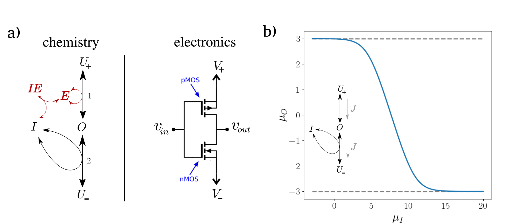
A chemical reaction network (CRN) is defined as a set of species and chemical reactions among these species. We consider as a demonstrative example the network in Fig. 1 a) (black part) that will be later analyzed in Sec. III.1:
| (1) |
There are four species connected by two chemical reactions; in the second, represents an enzyme. Physically, we imagine those species to be dissolved in a much more abundant inert solvent forming an ideal-dilute solution of volume . We assume that the time-scale in which the solute molecules diffuse is much shorter than that of chemical reactions. In this way, the solution can be considered homogenous at all times and the chemical concentrations represent the only out-of-equilibrium degrees of freedom. The states of the system are the ones corresponding to a given number of molecules for each chemical species,
| (2) |
The transition among those states occur through chemical reactions happening stochastically inside the solution. The resulting system’s dynamics is a Markovian jump-process. As we will see, stochasticity is a crucial ingredient for the Maxwell demon to function. The stochastic reaction rates obey the mass-action law: they are proportional to the product of the number of reactant molecules present in the solution,
| (3) |
where are the rate constants. The volume shows up to ensure .
For ideal-dilute solutions, where chemical concentrations are the only out-of-equilibrium degrees of freedom, the nonequilibrium chemical potential can be written as a function of the concentration in the form Rao and Esposito (2016); Alberty (2003)
| (4) |
The higher the concentration , the higher the chemical potential of . represents the standard chemical potential which depends on the solvent’s nature and on the temperature .
For an isolated CRN, the Gibbs free energy
| (5) |
decreases over time until the equilibrium value is reached Rao and Esposito (2016). This means that chemical reactions spontaneously proceed in the direction that reduces the chemical potential difference between reactants and products. When equilibrium is reached, for every reaction, the sum of the chemical potentials of the reactants must be equal to the sum of the chemical potentials of the products, which means, from Eq. (1),
| (6) |
If one combines this requirement with the fact that the equilibrium dynamics is detailed-balance and thus there are no net chemical currents,
| (7) |
one can derive the local detailed-balance conditions Rao and Esposito (2018)
| (8) |
This condition
guarantees the model’s thermodynamic consistency and it remains valid also for open CRNs.
Now, we move on to discuss open CRNs that can exchange chemical species with the environment. The CRN analyzed in this paper falls into this category and the reason for considering this kind of CRNs is that it simplifies the treatment: it allows one to remove some species from the dynamics by externally fixing their concentrations. We can imagine the system to be connected with chemical reservoirs, known as chemostats. Each chemostat can promptly exchange only one species with the system. Its size is assumed to be much bigger than the size of the system so that any perturbation induced by the evolution of the latter is effectively negligible.
By replenishing or taking away molecules, the net effect of each chemostat is to held the concentration (or equivalently the chemical potential) of the exchanged species constant in the system and equal to the chemostat’s value.
For example, in the CRN of Eq. (1), we can imagine to externally fix the concentration of the species by connecting the solution to two chemostats with chemical potentials . In the case , the system reaches a nonequilibrium steady state with a nonzero positive current flowing between the two chemostats. In the steady state, the free energy of the system is constant over time. However, free energy is being extracted at a rate in the chemostat and free energy is being released at a rate in the chemostat. The overall free energy consumed in stationary conditions is equal to the dissipation or entropy production rate Seifert (2012); Rao and Esposito (2018)
| (9) |
with .
In the following, all chemical potentials and free energies will be measured in units of .
III Chemical inverter
As mentioned in the introduction, the Maxwell demon is composed of two equivalent modules linked together. These modules can be thought of as chemical inverters. A good starting point for understanding the Maxwell demon is to follow a modular approach Avanzini et al. (2023): we first introduce and characterize the properties of a chemical inverter alone.
The CRN corresponding to the chemical inverter is shown in Fig. 1 a).
Its structure and working principle take inspiration from the CMOS electronic inverter Freitas and Esposito (2022) shown in the same figure. In the electronic case, the input potential controls the output potential . It does so through p-MOS and n-MOS transistors that act on the conductivity of the two channels connecting to the terminal potentials and , with . The name “inverter” stems from the fact that when is high, is low and vice versa. Indeed, if is high, what happens is that the p-MOS transistor blocks the upper channel, while the n-MOS transistor makes the lower channel very conductive, resulting in . If is low, the opposite happens, resulting in .
In the chemical case,
the input species is , the output species is , there are two internal species and two terminal species that can interconvert into through the upper and lower chemical reactions. In this context, the reaction rates and chemical potentials play, respectively, the roles of the conductivity and electric potentials. The terminal species and are considered to be chemostatted (Sec. II) to chemical potentials and , with . The input potential controls the output potential in an inverter-like manner by acting on the speed of the lower () and upper () chemical reactions. In the first case, this influence is made possible via the enzymatic reaction
| (10) |
The higher and therefore the concentration (Eq. (4)), the higher the rate at which this reaction takes place. This reproduces in chemistry the qualitative behavior of the n-MOS transistor: a higher results in a more conductive lower channel. In the second case, affects the upper reaction through the subnetwork
| (11) |
Whenever is high, the enzyme is converted into the inactive species , thus, slowing down the interconversion . This behavior represents the chemical analogue of the p-MOS transistor: a higher results in a less conductive upper channel.
Putting everything together, if is high, the lower reaction is much faster than the upper one. This translates into almost being in equilibrium with the lower species , which means . If, on the other hand, is low, the reverse happens and we have . We conclude that the CRN of Fig. 1 a) exhibits the qualitative inverter-like behavior.
We stress that both the electrical and chemical inverters must dissipate free energy in order to function. As a matter of fact, they need a nonzero potential difference applied to their terminals to be able to respond to an input signal. This potential difference translates, at steady state, into a nonzero electrical/chemical current flowing
from the higher to the lower electrical/chemical potential leading to a certain dissipation, which is given by Eq. (9) in the chemical case.
A final consideration is that the CRN of Fig. 1 a) still behaves as an inverter even without the “p-MOS subnetwork” (the red portion) 111 An electronic analog of this simplified version can be identified in the p-MOS inverter with load resistor Nair (2002).. This reduced CRN is simpler since there are no internal species and less symmetric because the input potential now only affects the speed of the lower reaction. Nevertheless, this simplified inverter is still sufficient for our goal of building a Maxwell demon and it greatly simplifies its analysis. Therefore, in the rest of the paper, we will consider this version.
III.1 Analysis of the simplified chemical inverter
The CRN corresponding to the simplified chemical inverter is the one already presented in Eq. (1):
| (12) |
In this Section, we quantitatively characterize its behavior. In particular, we find its steady state input-output relation. To this aim, we imagine that the input species and the terminal species are chemostatted respectively to chemical potentials , , (Sec. II). For convenience of notation, we filter out standard chemical potentials by setting . This is equivalent to measure relative to and , , relative to . In this way,
| (13) |
We assign the rate constants so that they are in compliance with the local detailed-balance conditions (8):
| (14) |
By substituting expressions (14) and (13) into Eq. (3) we get the stochastic rates:
| (15) |
The input-output relation is then obtained by the steady state condition, which requires the two average chemical currents to be equal
| (16) |
This leads to
| (17) |
Keeping in mind that is the concentration, we can recognize inside the parenthesis the Hill function Segel (1989) with Hill coefficient equal to 1. In Fig. 1 b), we plot this input-output relation. The behavior is the one expected for an inverter: for high , , while for low , . In the middle, there is a window of over which the inverter transitions between these two limiting cases. At steady state, to function, the inverter dissipates free energy from its chemostats at a rate given by Eq. (9)
| (18) |
The dissipation scales , the system size.
Finally, we mention in advance two more properties that will be used in the analysis of the Maxwell demon. They come from the fact that the stochastic process depicted in Eq. (15) is a 1D linear jump-process Gardiner (2009). Firstly, the relaxation rate for the mean is given by
| (19) |
Secondly, the steady state distribution is Poissonian Gardiner (2009) implying for the fluctuations
| (20) |
III.2 Chemical vs. electronic inverter
Before moving to the Maxwell demon, we go a little deeper in the comparison between the two kinds of inverter.
From a physical point of view, we already mentioned that
the analogues of electric potentials and conductivity are, in chemistry, chemical potentials and reaction rates.
Another physical distinction is that, contrary to the electronic case, in chemistry there is no spatial separation of components. With the assumption made in Sec. II, the chemical inverter is a homogeneous solution.
For what concerns the behavior of the two inverters, there is a crucial difference. In the electronic case, the steepness of the input-output curve can be increased by raising the powering voltage (Eq. (3) in Freitas and Esposito (2022)). This is not the case for the simplified and full chemical inverters where, after a certain point, an increase in is not reflected by an increase in the steepness. As a matter of fact,
the upper bounds on the nonequilibrium response found in Owen et al. (2020) apply to both type of chemical inverters setting a limit on their maximum steepness,
| (21) |
The derivation of those inequalities is explained in Appendix A. Their implications for the Maxwell demon will be explained in Sec. IV.
IV Chemical Maxwell demon
In this Section we introduce and study the chemical Maxwell demon.
We start with a preliminary overview where we discuss its structure, its qualitative thermodynamics, and working principle. A detailed quantitative analysis will follow.
Structure.
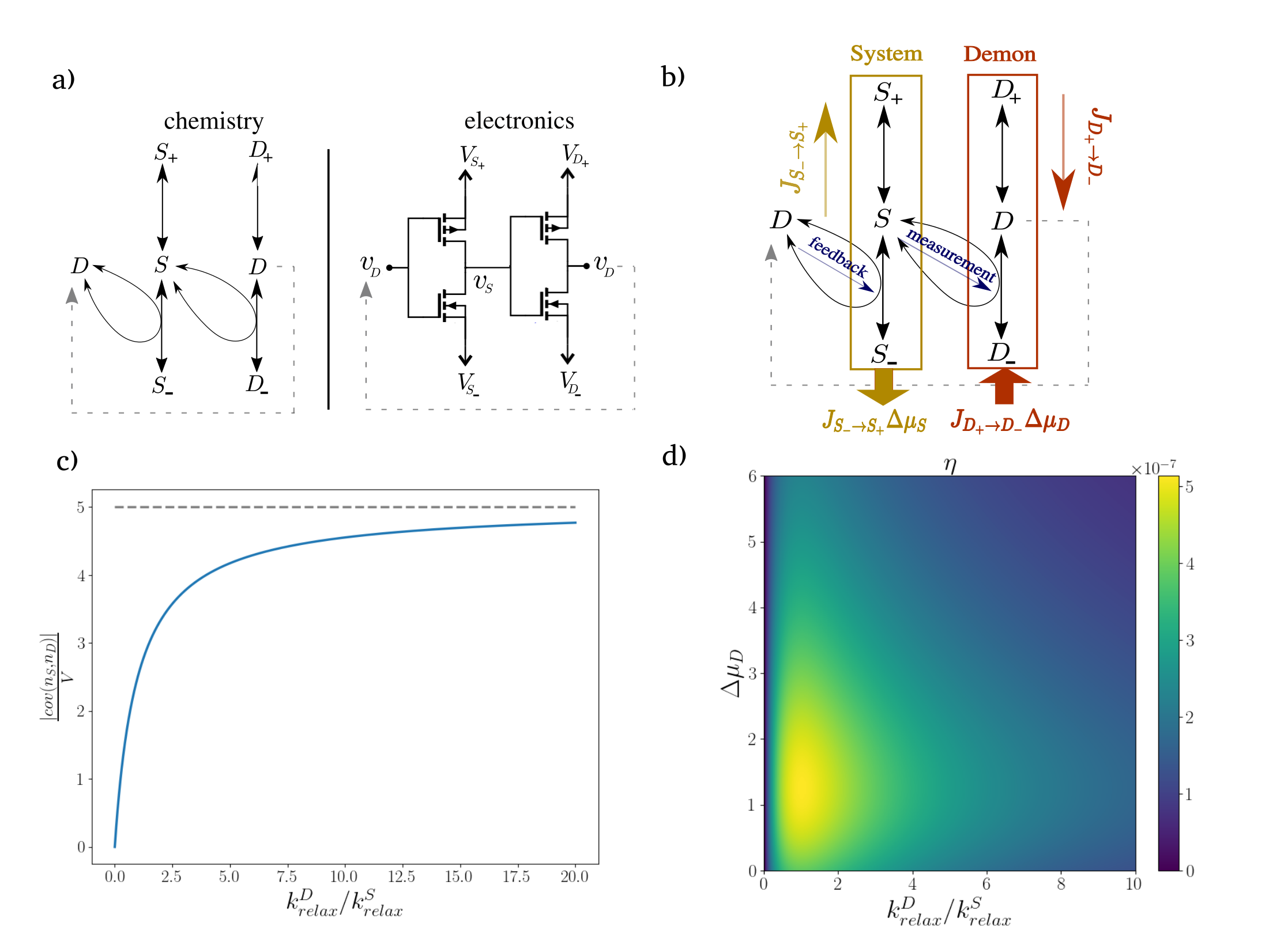
As in the electronic case Freitas and Esposito (2022), the Maxwell demon is obtained by combining two (simplified) chemical inverters.
In Fig. 2 a), the resulting MD CRN is contrasted with its electronic analogue.
In Fig. 2 b), the CRN’s structure is decomposed into its functions. One chemical inverter plays the role of the system and the other plays the role of the demon. While at the network level the demon and the system are distinct subnetworks, we notice again that they physically constitute the same homogeneous solution. This solution
contains six different chemical species: , which belong to the system, and , which pertain to the demon. The four terminal species are chemostatted: their concentrations are fixed so that the upper species (Fig. 2 b)) have higher chemical potentials, and . In this way, if we were to consider the system and the demon separately, we would expect the chemical reactions to proceed in the direction and .
Since these four species are chemostatted, we are left with only two dynamical species, which are and . Therefore, the global state is specified by the numbers of molecules : represents the state of the system, while the state of the demon. The global dynamics is a Markovian jump-process in this 2-D state space. The interaction between the system and the demon occurs through the two enzymatic reactions depicted in Fig. 2 b): is an enzyme for the demon’s inverter and is an enzyme for the system’s inverter. The peculiarity of enzymatic reactions is that they allow for a mutual influence between the two subnetworks without any exchange of energy. In fact, the only thing an enzyme does is to increase the rate of the catalyzed reaction by the same amount both in the forward and backward direction. Therefore, it does not push it in either direction leaving the reaction’s equilibrium unchanged.
The first enzymatic reaction, the one catalyzed by , can be interpreted as a way for the demon to collect information about the current state of the system and update its state accordingly. The second enzymatic reaction, the one catalyzed by , is the means by which the demon influences the system: based on its current state , which constitutes its internal representation (knowledge) of the system, the demon outputs a feedback on it.
Thermodynamics. As explained below, through the “measurement-feedback” mechanism just mentioned, the demon manages under certain conditions to create a reverse current in the system, Fig. 2 b). From Eq. (9), this current translates into free energy being generated in the system’s chemostats that can be equally seen as a local negative entropy production,
| (22) |
with . However, at the same time, the demon needs to consume free energy from its chemostats at a rate in order to do its job,
| (23) |
with . Since, from a global perspective, the following inequality holds true Horowitz and Esposito (2014),
| (24) |
the Maxwell demon as a whole is nothing but a free energy transducer that operates in compliance with the second law and the transduction efficiency is given by the ratio
| (25) |
The distinctiveness of this free energy transduction is that it is solely mediated by information exchange: enzymatic reactions, as mentioned above, do not lead to any energy exchange between the system and the demon.
This information flow and its precise link with the thermodynamics will be better discussed in Sec. IV.5.
Working principle.
How does the demon manage to generate a reverse current in the system? The working principle is analogous to the electronic case: it rectifies thermal fluctuations of chemical reactions.
To explain it, let’s assume for simplicity. In this condition, the system alone would reach an equilibrium with .
The demon can achieve by using a particular strategy:
at steady state, any particular fluctuation in the system’s number of molecules is expected on average to decay; based on the sign of , the demon can decide how it will relax.
If , the demon can “inhibit” the lower reaction by decreasing and making it easier for the excess of molecules to pour into , Fig. 2 b). If instead , the demon can boost the lower reaction by increasing and thus promoting the replenishment of missing molecules through the conversion . In both situations, an upward current is favored.
Therefore, we see that the essential ingredient to implement this strategy is to have anticorrelations between and .
But these anticorrelations are guaranteed by the fact that the demon behaves as an inverter, thus, “inverting” input fluctuations.
In the above reasoning, we are assuming that the demon is quick enough to readjust to system’s fluctuations before these ones actually decay. In Sec. IV.3, we will analyze the fallout from potential demon’s delays.
In conclusion, we see that the Maxwell demon’s mechanism manifest itself in
the correlations between the numbers of molecules.
However, in the limit , the covariance between these numbers goes to zero in relative terms.
As a consequence, the Maxwell demon effect becomes weaker and weaker until it disappears.
One way to prevent this is to increase the inverter’s steepness. A greater steepness allows for an amplification of small fluctuations as will be clarified in Sec. IV.1. By rescaling it properly, in principle, one could make the output of the MD survive in the large volume limit. This is exactly what was shown for the electronic demon Freitas and Esposito (2022). However, the same is not possible in the chemical case due to the bounds of Eq. (21).
To investigate how the performances of the chemical Maxwell demon scale with the system’s size, we perform its analysis at steady state focussing in the limit .
IV.1 Setup
In this paragraph, we assign the rates to the Maxwell demon; we describe how the macroscopic limit is performed; we mention the parameters that will allow us to rewrite the analytical results in a compact form; and, finally, we outline the strategy adopted to analytically solve the Maxwell demon.
The rate assignment is analogous to expression (15) both for the system and demon inverters:
| (26) |
| (27) |
In red and yellow, the influences of the enzymes and on the rates are highlighted.
As in Eq. (13), we measure with respect to and with respect to to filter out the standard chemical potentials of the and species. This rate assignment is in compliance with the local detailed balance condition (8), thus ensuring the thermodynamic consistency of the Maxwell demon’s model.
We denote with and respectively the system and demon’s concentrations,
| (28) |
The macroscopic limit is taken in the following manner:
| (29) |
The precise scaling of will be later derived, Eq. (41). The reason why is that the Maxwell demon effect becomes weaker and weaker, thus allowing to overcome decreasing chemical gradients . In the limit , the deterministic concentrations of the and species are, from Eq. (17):
| (30) |
We denote as the working point.
In the following, three quantities will turn out to be particularly useful for interpreting the analytical results: the two inverter relaxation rates and the fluctuation-amplifying factor .
The inverter relaxation rates are approximately given by Eq. (19) evaluated in the macroscopic limit
| (31) |
The fluctuation-amplifying factor can be introduced through the function that corresponds to the steady state input-output relation of the demon inverter rewritten in terms of number of molecules. In other words, is the average number of molecules assuming that the number of molecules is kept fixed at the value . From Eq. (17), it is
| (32) |
The fluctuation-amplifying factor is then defined as
| (33) |
Put into words, is the factor by which small fluctuations around the working point get amplified by the demon’s inverter assuming it reacted instantaneously. In principle, we would like to increase as much as possible: the bigger it is, the stronger the Maxwell demon effect. However, the inequality for the steepness of the input-output relation (21) sets an upper bound to its value:
| (34) |
We now present the strategy adopted to solve the Maxwell demon. At steady state, one must have for each inverter equal upper and lower average currents, and (see Fig.2 b)), and therefore:
| (35) |
and
| (36) |
From the left-hand side of the above expressions, we see that , and thus the efficiency , Eq. (25), can be obtained once we know and . In particular, since scales , it can be calculated approximating . Using Eq.(30) for and substituting inside Eq.(36) leads to
| (37) |
Notice that and thus the free energy consumed by the demon is also , the fluctuation-amplifying factor. To calculate , we need to be more careful as it has a much smaller value: differently from , it turns out to be intensive in the volume.
| (38) |
Therefore, the same approximation that would be right to
obtain the zeroth order of the current fails to give a correct result for .
To obtain this value, we would need to calculate with higher accuracy, up to order .
The procedure we will follow involves two steps: first, we show that we can link and thus all the quantities characterizing the Maxwell demon performances to the covariance ; secondly, we calculate the latter through a Gaussian approximation of the rate function.
Note that a more straightforward approach in which one uses the Gaussian approximation to directly calculate is wrong. In general, the Gaussian approximation is not accurate
enough for first order moments, while it is for second order moments, like . See Appendix B for a discussion.
IV.2 Maxwell demon’s quantities as a function of
The covariance emerges as a pivotal variable. In this paragraph, we link and all the other quantities describing the Maxwell demon performances to it. This allows us to address the scaling behavior of those quantities from the expected scaling
| (39) |
as the covariance is additive for independent systems. This scaling will be later confirmed in Eq. (48). Firstly, we establish the relationship between and . We do it through Eq. (35) working up to first order in and . Calculations are reported in Appendix C; the result is
| (40) |
The last factor on the right-hand side is adimensional and only depends on the system’s rates. Interestingly, the reverse current generated by the Maxwell demon is proportional to , which is partly due to the fact that the interaction between and occurs through two-body reactions (i.e. the enzymatic reactions). Because of Eq. (39), we see that is intensive, it does not vary with the system’s size. From expression (40), we also see that the effective reverse affinity created in the system is equal to
| (41) |
represents the range of vincible chemical gradients. It goes to zero in the deterministic limit.
Having connected the current to the covariance , we can do the same for the output power , Eq. (22), and the efficiency , Eq. (25). One obtains
| (42) |
and
| (43) |
The efficiency and the output power are quadratic functions of and they are both maximized by
| (44) |
This optimal value leads to
| (45) |
and
| (46) |
The optimal output power and efficiency turn out to be proportional to the square of the covariance and their scaling, from Eq. (39), is respectively and . This is due to the fact that the opposite chemical gradient is plus, for the efficiency, the fact that the current in the demon’s inverter is . In Table 1, we summarize these scalings characterizing the Maxwell demon; they are analogous to the ones found for the electronic version Freitas and Esposito (2022, 2023).
| Quantity | Scaling |
|---|---|
| , cov(,), | |
| , | intensive |
| , , , | |
IV.3
As explained in Appendix B, can be determined with a sufficient accuracy from the Gaussian approximation of the rate function. This approximation can be derived, as was done in Freitas and Esposito (2022), from the master equation of the 2D jump-process. The schematic procedure consists in, firstly, substituting
| (47) |
in the master equation and, secondly, solving the resulting equation for , the covariance matrix. The details are reported in Appendix D. The final result is
| (48) |
In Fig. 2 c), we plot it as a function of the time-scale separation between the demon and the system.
When , we are in the fast demon limit: the demon inverter responds instantaneously to changes in according to Eq. (32). Since fluctuations around the working point are small when , the demon’s response can be actually approximated with the linear part of Eq. (32):
| (49) |
and the covariance between and arising from such a response is 222We use the fact that, in the absence of the small perturbation introduced by the demon feedback, would be a Poissonian with average .
| (50) |
which is in agreement with the value given by Eq. (48).
On the other hand, when , the demon becomes very slow and its delay results in weaker correlations:
tries to update its state based on that of , but since it is slow, may change in the meantime. This is confirmed from Eq. (48)
| (51) |
From Eq. (40) and (41), the weaker the correlations, the lower the reverse current and the affinity produced in the system. In other words, this delay makes the demon feedback on the system anachronistic and thus less effective.
IV.4 Efficiency
With the covariance calculated in the previous paragraph, we can obtain an explicit expression for the efficiency of Eq. (46). The result is
| (52) |
A plot of as a function of and the time-scale separation between the demon and the system is shown in Fig. 2 d). When , because of the negative impact of the demon’s delay. Also, when , : the demon answers promptly to any system’s change but, in order to do so, it consumes an increasing amount of free energy . From Eq. (52), the efficiency is maximized when the time-scales of the two inverters are equal: . When , : after a certain point, an increase in the demon powering voltage does not translate into an increase of (Eq. (34)) and leads only to more free energy being dissipated. From the plot, we see that the efficiency is maximized for a nonzero . Its maximum value can be upper-bounded exploiting the inequality (34) and the fact that the right-most adimensional parentheses of Eq. (52) is .
| (53) |
The maximum value is very low as it is inversely proportional to the product of the numbers of and molecules present in the solution. For example, in biological conditions, imagining and to be proteins inside a cell with , we would have .
IV.5 Maxwell demon thermodynamics with information flow
In Section IV, we presented the basic Maxwell demon
thermodynamics and we highlighted the absence of any energy exchange between the two inverters.
In this Section, we dive deeper analyzing the Maxwell demon with the formalism of bipartite systems Horowitz and Esposito (2014); Hartich et al. (2014).
This framework allows one to further resolve
its thermodynamics. In particular, two separate second laws can be obtained for the two inverters. They include a new term, the information flow, that quantifies the rate at which information is exchanged between the system and the demon. Thanks to these refined second laws, it is possible to decompose the global efficiency, Eq. (25), as the
product of two efficiencies related respectively to the demon and the system, or equivalently, to the measurement and feedback processes. In this section, we first explain how the bipartite formalism applies to our chemical MD and then evaluate the information flow, which allows us to discuss the behavior of the two efficiencies above mentioned.
We begin by stating in which sense the Maxwell demon is bipartite: it is composed of two degrees of freedom, which are the state of the system and the state of the demon ; in addition, the possible chemical reactions change either or but not both at the same time. This last property enables a decomposition of the time derivative of the mutual information
| (54) |
into two pieces: one due to reactions changing the state of the system and the other due to reactions changing the state of demon:
| (55) |
with
| (56) |
In these expressions, represents the net average current along the transition and is defined analogously. In stationary conditions, one must have
| (57) |
We call the information flow from the demon to the system. As anticipated, for bipartite systems, it is possible to derive two refined second laws valid for each subpart that take into account this quantity Horowitz and Esposito (2014). They read
| (58) |
where is the steady state local dissipation rate of the system/demon inverter defined in Eq. (22)/(23). These two inequalities embody the thermodynamic understanding of a Maxwell demon: the demon produces mutual information (correlations), , by adjusting its state according to that of the system. However, to do this, it needs to dissipate a certain amount of free energy . This generated mutual information is subsequently burned by the system allowing for a negative local dissipation , which corresponds to free energy being extracted from the system. The sum of both inequalities of Eq. (58),
| (59) |
ensures that the Maxwell demon as a whole operates in compliance with the second law.
The refined second laws, Eq. (58), also allow us to decompose the overall transduction efficiency, Eq. (25), into two partial efficiencies:
| (60) |
The partial efficiency measures how efficiently the demon converts the consumed free energy into new mutual information, while is the efficiency with which the system burns mutual information to release free energy in its chemostats. and can be, respectively, thought of as the efficiencies of the measurement and feedback step, and are less or equal to one, by virtue of the inequalities in Eq. (58).
in the chemical Maxwell demon
We derive analytically for a fast demon and we find its qualitative behavior in the case of a slow demon. Finally, we display the information flow pattern in the state space.
In the limit , it is simpler to derive . For the sake of its derivation, we can also assume . As a matter of fact, can be considered with good approximation constant over the small range of vincible chemical potential gradients , Eq. (41).
We compute from , Eq. (56). For this, the knowledge of the steady state conditional probability distribution is required.
In the fast demon limit, this distribution can be approximated with a Poissonian (see the end of Sec. III.1) with average given by Eq. (32). The detailed calculations are reported in Appendix E.1. The result is
| (61) |
We notice that is an intensive quantity: it does not scale with the volume . We can combine its expressions with that of , Eq. (40), to obtain the partial efficiency in Eq. (60). This partial efficiency is maximum for the same that maximized , Eq. (44).
| (62) |
From the above expression, we see that the partial efficiency with which the system converts mutual information into output free energy scales . Knowing from Eq. (46) that , we conclude that (see Table 1 for a summary).
To make the discussion more exhaustive, we can qualitatively analyze the opposite case of a very slow demon
. In this limit, we know through Eq. (52) that and
we can ask ourselves whether this inefficiency is due to or . To answer this question, it is necessary to know how the information flow scales. In Appendix E.2, we show that its scaling is
| (63) |
Therefore, in the limit of a slow demon, keeping in mind that and , the partial efficiencies scale as
| (64) |
This means that the loss in efficiency is due to the measuring step: as the demon becomes slower, due to delays, it converts much less effectively consumed free energy into mutual information.
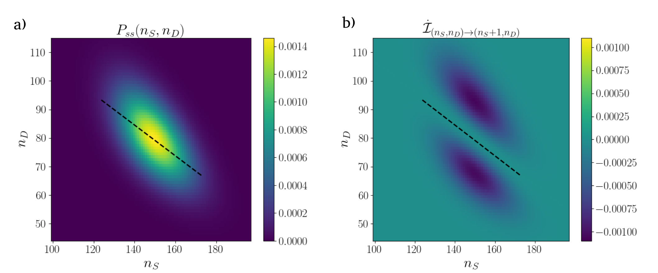
We conclude the section by discussing the information flow pattern in the state space. As a matter of fact, from Eq. (56), we see that we can break down into a sum of contributions coming from each individual transition
| (65) |
We can then visualize these contributions by plotting them in the state space: in point we show the value . The plot, together with that of , is shown in Fig. 3. The probability distribution is a rotated ellipsoid, denoting correlations between and . is everywhere negative, meaning that the system is consuming mutual information.
The main contributions to arise from the two regions close to the center that are adjacent to the line of Eq. (49). We can elucidate the pattern in the following way.
States starting from the line, where is concentrated (Fig. 3 a)), diffuse horizontally to the left/right of the dotted line due to random transitions in the system’s inverter. This horizontal dilution has the effect of destroying correlations between and
and, consequently, of reducing mutual information.
However, the demon counteracts this horizontal spreading by
vertically absorbing back into the line those escaping states. In this way, the demon is generating in those two regions above/below the line new mutual information that compensates the one burned by the system in the same two regions.
V Conclusions
In this article, we studied the chemical analog of an electronic Maxwell demon. We examined in detail its structure and working principle (Sec. IV).
We highlighted the correlations between the numbers of molecules as the central quantity that captures the essence of the MD (Sect. IV.2).
We conducted a thorough characterization of the system’s scaling in the macroscopic limit, summarized in Table 1, and examined the Maxwell demon’s efficiency in relation to the time-scale separation of the two inverters, the demon powering chemical potential, and the opposing chemical gradient (Sec.IV.4).
Finally, the bipartite formalism allowed us to enlighten the details of its thermodynamics through the information flow (Sec. IV.5).
The system presents some inconveniences:
its efficiency is found to be extremely low (Eq. 53) and it is not possible to make the MD’s output survive in the macroscopic limit even by increasing the input power.
Nevertheless, this system enriches
our understanding of information-mediated transduction in CRNs and represents a first step towards unveiling deeper connections between electronics and chemistry. Regarding the latter point, we believe it worthwhile to push further the two approaches followed in this paper: the electronics-inspired design of CRNs and their analysis from a modular perspective Avanzini et al. (2023) analogous to the one developed for electronic circuits.
VI Acknowledgements
We thank Francesco Avanzini and Emanuele Penocchio for useful discussions.
This is research was supported by AFR PhD grant 15749869 and by project ChemComplex
(C21/MS/16356329) funded by Luxembourg National
Research Fund (FNR) (Luxembourg), and by project
no. INTER/FNRS/20/15074473 funded by FRS-FNRS
(Belgium) and FNR (Luxembourg).
For open access, the author has applied a Creative Commons Attribution 4.0 International (CC BY 4.0) license to any Author Accepted Manuscript version arising from this submission.
Appendix A Bounds on the chemical inverter steepness
The first bound in (21) can be shown by computing from Eq. (17)
| (66) |
The last inequality can be verified directly through calculations. Alternatively, one can recognize that the inverter falls in the range of application of Owen et al. (2020) (Sec. VI). The second bound in (21) can be proved by applying the chain rule. Indeeed, the output chemical potential in the full inverter, Fig. 1 a), can be envisaged as the function
| (67) |
and we can use the chain rule to obtain the total derivative of with respect to
| (68) |
, in analogy with , is . Moreover, at steady state one must have
| (69) |
plus the relation coming from the conservation law
| (70) |
The two together leads to
| (71) |
Putting everything back into Eq. (68), we conclude
| (72) |
Appendix B Accuracy of the Gaussian approximation
In this Appendix, we show that the Gaussian approximation of the rate function is not sufficient to calculate first order moments up to order , like , while it is for second order moments, like , up to the same accuracy.
For simplicity, we limit the discussion to the 1D case. Analogous results can be found for the 2D case, which is our case.
Consider a system described by an intensive variable that in our case would be the concentration of the species and by a scale parameter V, the volume.
Assume, as in our situation, that the exact steady state distribution has the following scaling behavior
| (73) |
with
| (74) |
The first term on the right-hand side, , is called the rate function and can be derived from the master equation of the process by inserting and ignoring terms of lower order in . The value , where the rate function has its minimum , represents the deterministic value approached in the limit . The Gaussian approximation consists in retaining only the rate function from the right-hand-side of Eq. (74) and expanding it up to second order around
| (75) |
with .
We now show that this approximation is too drastic if one wants to calculate with accuracy . We do so by pointing out that the next order correction gives nonnegligible contributions.
To obtain a probability distribution correct up to order , the third order expansion of and the term are needed. If we keep them, the improved approximation reads
| (76) |
In the relevant region where is not zero, which is increasingly smaller as , we can approximate . Moreover, in the same region, we can bring down the argument of the exponential since it is . From the normalization condition, it is and we can write
| (77) |
If we use it to calculate , we get
| (78) |
where the mean values are computed with respect to . Thus, we realize that and the third order expansion of give relevant contributions of order . On the other hand, if we are interested in , is sufficient as the next order correction gives zero contribution:
| (79) |
Notice that if thanks to the symmetry of the problem, is known to be even with respect to , then and is accurate enough for calculating . This is what happens in the electronic Maxwell demon Freitas and Esposito (2022) if all the transistors involved are assumed to have the same parameters.
Appendix C obtaining in terms of
Appendix D Evaluation of
We here derive the guassian approximation of the stationary probability distribution. From that, we obtain the covariance. We adopt exactly the same methodology used in Freitas and Esposito (2022).
The master equation of the 2D jump-process is
| (82) |
, the index represents the possible transitions, and is the net change in the state of the Maxwell demon as a result of the transition . There are two possible transitions that change the number of molecules in the system, , and two possible transitions changing the number of molecules in the demon, .
As a preliminary step, we can substitute in the stationary master equation, with . One gets disregarding terms sublinear in the volume
| (83) |
where are the rescaled rates. Then, we can proceed substituting the gaussian approximation in Eq. (83), with . We obtain the following equation for the covariance matrix
| (84) |
with
| (85) |
and
| (86) |
Eq. (84) can be explicitly solved for yielding
| (87) |
Appendix E Information flow
E.1 in the limit of a fast demon
We obtain Eq. (61) starting from Eq. (56). We perform calculations setting as justified in the text.
| (88) | ||||
In this regime, is a Poissonian with mean given by Eq. (32). In the large volume limit, can be approximated by the linear relation Eq. (49). This leads to
| (89) |
The last term on the right-hand side is a constant and it gives zero contribution to Eq. (88) since
| (90) |
This equality comes from the fact that the barycenter of a steady state distribution does not move horizontally. The term enters in Eq. (88) together with
| (91) | ||||
To obtain the final result
| (92) |
one takes the average with respect to , firstly, and with respect to , secondly: is given by the linear relation (49) and can be approximated in this context with .
E.2 Scaling of in the limit of a slow demon
We call . With , one has
| (93) |
Put into words: the rates of the system are infinitely faster than those of the demon, thus, for any given , the system equilibrates with respect to to a distribution that, due to , is actually independent of . In particular, is a Poissonian with average . Therefore, in this limit, the steady state probability ditribution factorizes and we can write to next order in
| (94) |
The information flow can be evaluated from Eq. (56) as
| (95) |
Around the working point, from where the major contributions to come from, the current along scales
| (96) |
and from Eq. (94),
| (97) |
so that
| (98) |
Combining Eq. (96) and (98), we have
| (99) |
as claimed in the text.
References
- Maxwell (1871) James Clerk Maxwell, Theory of Heat (Longmans, Green, and Co., London, UK, 1871) Chap. 12.
- Leff and Rex (2002) Harvey Leff and Andrew F Rex, Maxwell’s Demon 2 Entropy, Classical and Quantum Information, Computing (CRC Press, 2002).
- Szilard (1929) Leo Szilard, “On the decrease of entropy in a thermodynamic system by the intervention of intelligent beings,” Zeitschrift für Physik 65, 840–866 (1929).
- Brillouin (1951) L. Brillouin, “Maxwell’s demon cannot operate: Information and entropy,” Journal of Applied Physics 22, 334–337 (1951).
- Landauer (1961) R. Landauer, “Irreversibility and heat generation in the computing process,” IBM Journal of Research and Development 5, 183–191 (1961).
- Landauer (1991) R. Landauer, “Information is physical,” Physics Today 44, 23–29 (1991).
- Bennett (1982) Charles H. Bennett, “The thermodynamics of computation—a review,” International Journal of Theoretical Physics 21, 905–940 (1982).
- Sagawa and Ueda (2009) Takahiro Sagawa and Masahito Ueda, “Minimal energy cost for thermodynamic information processing: Measurement and information erasure,” Phys. Rev. Lett. 102, 250602 (2009).
- Cao and Feito (2009) F. J. Cao and M. Feito, “Thermodynamics of feedback controlled systems,” Phys. Rev. E 79, 041118 (2009).
- Sagawa and Ueda (2012) Takahiro Sagawa and Masahito Ueda, “Nonequilibrium thermodynamics of feedback control,” Phys. Rev. E 85, 021104 (2012).
- Esposito and Schaller (2012) Massimiliano Esposito and Gernot Schaller, “Stochastic thermodynamics for “maxwell demon” feedbacks,” Europhysics Letters 99, 30003 (2012).
- Barato and Seifert (2014) A.C. Barato and U. Seifert, “Unifying three perspectives on information processing in stochastic thermodynamics,” Physical Review Letters 112, 090601 (2014).
- Serreli et al. (2007) Viviana Serreli, Chin-Fa Lee, Euan R Kay, and David A Leigh, “A molecular information ratchet,” Nature 445, 523–527 (2007).
- Alvarez-Pérez et al. (2008) Mónica Alvarez-Pérez, Stephen M. Goldup, David A. Leigh, and Alexandra M. Z. Slawin, “A chemically-driven molecular information ratchet,” Journal of the American Chemical Society 130, 1836–1838 (2008).
- Carlone et al. (2012) Armando Carlone, Stephen M Goldup, Nathalie Lebrasseur, David A Leigh, and Adam Wilson, “A three-compartment chemically-driven molecular information ratchet,” J Am Chem Soc 134, 8321–8323 (2012).
- Amano et al. (2022) Shuntaro Amano, Massimiliano Esposito, Elisabeth Kreidt, David A. Leigh, Emanuele Penocchio, and Benjamin M. W. Roberts, “Insights from an information thermodynamics analysis of a synthetic molecular motor,” Nature Chemistry 14, 530–537 (2022).
- Toyabe et al. (2010) Shoichi Toyabe, Takahiro Sagawa, Masahito Ueda, Eiro Muneyuki, and Masaki Sano, “Experimental demonstration of information-to-energy conversion and validation of the generalized jarzynski equality,” Nature Physics 6, 988–992 (2010).
- Saha et al. (2021) Tushar K. Saha, Joseph N. E. Lucero, Jannik Ehrich, and John Bechhoefer, “Maximizing power and velocity of an information engine,” Proceedings of the National Academy of Sciences 118, e2023356118 (2021).
- Bannerman et al. (2009) S Travis Bannerman, Gabriel N Price, Kirsten Viering, and Mark G Raizen, “Single-photon cooling at the limit of trap dynamics: Maxwell’s demon near maximum efficiency,” New Journal of Physics 11, 063044 (2009).
- Kumar et al. (2018) Aishwarya Kumar, Tsung-Yao Wu, Felipe Giraldo, and David S Weiss, “Sorting ultracold atoms in a three-dimensional optical lattice in a realization of maxwell’s demon,” Nature 561, 83–87 (2018).
- Koski et al. (2014) Jonne V. Koski, Ville F. Maisi, Jukka P. Pekola, and Dmitri V. Averin, “Experimental realization of a szilard engine with a single electron,” Proceedings of the National Academy of Sciences 111, 13786–13789 (2014).
- Koski et al. (2015) J. V. Koski, A. Kutvonen, I. M. Khaymovich, T. Ala-Nissila, and J. P. Pekola, “On-chip maxwell’s demon as an information-powered refrigerator,” Phys. Rev. Lett. 115, 260602 (2015).
- Camati et al. (2016) Patrice A. Camati, John P. S. Peterson, Tiago B. Batalhão, Kaonan Micadei, Alexandre M. Souza, Roberto S. Sarthour, Ivan S. Oliveira, and Roberto M. Serra, “Experimental rectification of entropy production by maxwell’s demon in a quantum system,” Phys. Rev. Lett. 117, 240502 (2016).
- Vidrighin et al. (2016) Mihai D. Vidrighin, Oscar Dahlsten, Marco Barbieri, M. S. Kim, Vlatko Vedral, and Ian A. Walmsley, “Photonic maxwell’s demon,” Phys. Rev. Lett. 116, 050401 (2016).
- Cottet et al. (2017) Nathanaël Cottet, Kuan Y. Tan, Riccardo Pisoni, Marc Ganzhorn, Eva Dupont-Ferrier, Andreas Wallraff, Christian Schönenberger, and Lieven M. K. Vandersypen, “Observing a quantum maxwell demon at work,” Proceedings of the National Academy of Sciences 114, 7561–7564 (2017).
- Masuyama et al. (2018) Y. Masuyama, K. Funo, Y. Murashita, A. Noguchi, S. Kono, Y. Tabuchi, R. Yamazaki, M. Ueda, and Y. Nakamura, “Information-to-work conversion by maxwell’s demon in a superconducting circuit quantum electrodynamical system,” Nature Communications 9, 1291 (2018).
- Naghiloo et al. (2018) M. Naghiloo, J. J. Alonso, A. Romito, E. Lutz, and K. W. Murch, “Information gain and loss for a quantum maxwell’s demon,” Phys. Rev. Lett. 121, 030604 (2018).
- Ribezzi Crivellari and Ritort (2019) Marco Ribezzi Crivellari and F. Ritort, “Large work extraction and the landauer limit in a continuous maxwell demon,” Nature Physics 15, 1 (2019).
- Najera-Santos et al. (2020) Baldo-Luis Najera-Santos, Patrice A. Camati, Valentin Métillon, Michel Brune, Jean-Michel Raimond, Alexia Auffèves, and Igor Dotsenko, “Autonomous maxwell’s demon in a cavity qed system,” Phys. Rev. Res. 2, 032025 (2020).
- Freitas and Esposito (2022) Nahuel Freitas and Massimiliano Esposito, “Maxwell demon that can work at macroscopic scales,” Phys. Rev. Lett. 129, 120602 (2022).
- Freitas and Esposito (2023) Nahuel Freitas and Massimiliano Esposito, “Information flows in macroscopic maxwell’s demons,” Phys. Rev. E 107, 014136 (2023).
- Flatt et al. (2021) Solange Flatt, Daniel M. Busiello, Stefano Zamuner, and Paolo De Los Rios, “Abc transporters are billion-year-old maxwell demons,” bioRxiv (2021), 10.1101/2021.12.03.471046.
- Penocchio et al. (2022) Emanuele Penocchio, Francesco Avanzini, and Massimiliano Esposito, “Information thermodynamics for deterministic chemical reaction networks,” The Journal of Chemical Physics 157, 034110 (2022).
- Seifert (2012) Udo Seifert, “Stochastic thermodynamics, fluctuation theorems, and molecular machines,” Reports on Progress in Physics 75, 126001 (2012).
- Schmiedl and Seifert (2007) Tim Schmiedl and Udo Seifert, “Stochastic thermodynamics of chemical reaction networks,” The Journal of Chemical Physics 126, 044101 (2007).
- Rao and Esposito (2016) Riccardo Rao and Massimiliano Esposito, “Nonequilibrium thermodynamics of chemical reaction networks: Wisdom from stochastic thermodynamics,” Phys. Rev. X 6, 041064 (2016).
- Horowitz and Esposito (2014) Jordan M. Horowitz and Massimiliano Esposito, “Thermodynamics with continuous information flow,” Phys. Rev. X 4, 031015 (2014).
- Hartich et al. (2014) David Hartich, Andre Barato, and Udo Seifert, “Stochastic thermodynamics of bipartite systems: Transfer entropy inequalities and a maxwell’s demon interpretation,” Journal of Statistical Mechanics: Theory and Experiment 2014 (2014), 10.1088/1742-5468/2014/02/P02016.
- Rao and Esposito (2018) Riccardo Rao and Massimiliano Esposito, “Conservation laws and work fluctuation relations in chemical reaction networks,” The Journal of Chemical Physics 149, 245101 (2018).
- Alberty (2003) R. A. Alberty, Thermodynamics of Biochemical Reactions (Wiley-Interscience, New York, 2003).
- Avanzini et al. (2023) Francesco Avanzini, Nahuel Freitas, and Massimiliano Esposito, “Circuit theory for chemical reaction networks,” Phys. Rev. X 13, 021041 (2023).
- Note (1) An electronic analog of this simplified version can be identified in the p-MOS inverter with load resistor Nair (2002).
- Segel (1989) Lee A. Segel, Enzyme Kinetics: Behavior and Analysis of Rapid Equilibrium and Steady-State Enzyme Systems (Wiley-Interscience, New York, 1989).
- Gardiner (2009) Crispin Gardiner, Stochastic Methods: A Handbook for the Natural and Social Sciences, Springer Series in Synergetics (Springer Berlin, Heidelberg, 2009).
- Owen et al. (2020) Jeremy A. Owen, Todd R. Gingrich, and Jordan M. Horowitz, “Universal thermodynamic bounds on nonequilibrium response with biochemical applications,” Phys. Rev. X 10, 011066 (2020).
- Note (2) We use the fact that, in the absence of the small perturbation introduced by the demon feedback, would be a Poissonian with average .
- Nair (2002) B. Somanathan Nair, Digital Electronics and Logic Design (PHI Learning Pvt. Ltd., 2002) p. 240.