Review on the decoding algorithms for surface codes

Abstract

Quantum technologies have the potential to solve computationally hard problems that are intractable via classical means. Unfortunately, the unstable nature of quantum information makes it prone to errors. For this reason, quantum error correction is an invaluable tool to make quantum information reliable and enable the ultimate goal of fault-tolerant quantum computing. Surface codes currently stand as the most promising candidates to build near term error corrected qubits given their two-dimensional architecture, a requirement of only local operations, and high tolerance to quantum noise. Decoding algorithms are an integral component of any error correction scheme, as they are tasked with producing accurate estimates of the errors that affect quantum information, so that it can subsequently be corrected. A critical aspect of decoding algorithms is their speed, since the quantum state will suffer additional errors with the passage of time. This poses a connundrum-like tradeoff, where decoding performance is improved at the expense of complexity and viceversa. In this review, a thorough discussion of state-of-the-art surface code decoding algorithms is provided. This work is oriented to readers which may be introducing themselves within the field or willing to further their understanding of the relevant decoders for the surface code, as well as of the state-of-the-art of the field. The core operation of these methods is described along with existing variants that show promise for improved results. In addition, both the decoding performance, in terms of error correction capability, and decoding complexity, are compared. A review of the existing software tools regarding surface code decoding is also provided.

Quantum error correction, surface codes, decoherence

1 Introduction

Significant progress has been made in the field of quantum computing since Feynman first introduced the idea of computers that use the laws of quantum mechanics in 1982 [1]. Quantum computers leverage the principles of quantum mechanics to accelerate computational processes that are deemed as intractable by means of classical machines, leading to unprecedented results [2]. This technology presents an unprecedented potential to solve problems that are computationally hard since algorithms that present an exponential speedup in terms of computational complexity have been theoretically proposed [3, 4]. In this sense, these novel processors are expected to revolutionize the modern society by improving applications related to cryptography [5, 6], optimization [7, 8, 9], macromolecule design [10, 11, 12] or basic science [13, 14], among others. Recently, quantum supremacy or advantage has been experimentally proven [15, 16, 17, 18, 19], thus, demonstrating that the potential promised by the theory can indeed be realized in physical machines.

There are many possible paths towards the construction of quantum processors such as qubit gate-based quantum computing [20], qudit-based quantum computing [21], measurement based quantum computing [22, 23], quantum annealers [24] or bosonic quantum computing [25], to name a few. Additionally, many physical implementations of these types of technologies like superconducting circuits [26], ion-traps [27] or photons [28] are currently being investigated. In the present article, we will restrict our discussion for qubit gate-based quantum computation, in which the physical elements are realized by discrete two-level systems.

Nevertheless, quantum noise stands as a big obstacle in the way of the groundbreaking promise that quantum technologies offer theoretically [29, 30]. The qubits which constitute quantum computers are prone to suffer from errors, implying that the computations being performed are inaccurate and, therefore, unuseful. The errors that arise whenever computations are being performed via qubits have many origins [30]. For example, quantum gates, which are the quantum analogue of logic gates of classical computation, may introduce unwanted errors to the quantum states being processed due to the fact an over- or under-rotation is being done due to the lack of precision of the elements used for doing such gates [31]. Many of the errors arise due to similar limits in the equipment being used for preparing , controlling or measuring such quantum mechanical systems, and it may seem that dealing with errors suffered by qubits is an engineering problem [32, 33]. However, these elements do also suffer from errors whose origin is their inescapable interaction with their surrounding environment [30, 34, 35]. These types of errors, which are grouped under the term decoherence, constitute a very problematic error source since they always exist. However, dealing with errors is no new feature in the field of computer science [36, 37, 38]. The study of methods for preventing the effects of noise in classical computers is a rich subject area which follows us to the time being, being present in commodities so important as WiFi and other communication devices. Unfortunately, phenomena particular to the quantum mechanics field such as the no-cloning theorem or the effects of measurement in a quantum state prevent several classical methods to be implemented seamlessly in the quantum realm. Luckily, quantum error correction (QEC) was demonstrated to be possible theoretically when the 9-qubit Shor code was proposed in 1995 [29] and generalized afterwards with the theory of Quantum Stabilizer Codes (QSC) by Gottesman in his PhD thesis [39]. The field of quantum error correction has advanced significantly since its earliest formulation and several families of quantum error correction codes (QECC) such as Topological codes [32, 40, 41, 42, 43, 44], Quantum Low-Density Parity Check (QLDPC) codes [45, 46, 47, 48, 49, 50] or Quantum Turbo Codes (QTC) [51, 52, 53], for example, have been proposed.

The basic idea behind quantum error correction can be understood as having the information of a set of qubits (logical qubits) encoded in a greater number of qubits (physical qubits) via a mapping named encoding [30, 39, 54]. In order to estimate the errors suffered from those qubits, a non-destructive measurement (with this we mean that the actual qubits constituting the code are not directly measured) named syndrome measurement is done so that useful information about such error is retrieved [30]. The obtained syndrome is then used so that an error candidate for returning the code to the previous undamaged state is estimated. This process, referred as syndrome decoding depends on the specific code construction [32, 41, 42, 43, 44, 45, 46, 47, 48, 49, 50, 51, 52, 53] and is a critical task for the QECCs to work correctly. Decoding quantum error correction codes is a subtle task due to a quantum unique effect named code degeneracy [46, 54], which refers to the existence of errors that share the same syndrome, but transform the quantum state in an indistinguishable manner. As a consequence of degeneracy, the optimal decoding of stabilizer codes has been proven to belong to the $\#$P-complete complexity class, which is computationally much harder than decoding classical linear codes [54, 55]. This high complexity imposes a trade-off between decoding performance and decoding time, as related to complexity of the decoding algorithm, due to the fact that decoders of quantum error correction codes should be fast enough in order to correct the noisy quantum state before it suffers from more errors or decoheres completely [56, 57]. Therefore, the field of constructing more efficient, in terms of speed and correction performance, decoders for stabilizer codes is a very active and relevant field of quantum error correction.

Surface codes are one of the most promising families of codes for constructing primitive fault-tolerant quantum computers in the near-term [32, 40, 58, 59, 60, 61, 62]. This family of topological codes presents the benefit of being implementable in two-dimensional grids of qubits with local syndrome measurements, or check operators in the surface code terminology, while presenting a high tolerance to quantum noise [59]. Considering that many of the physical platforms being considered for constructing quantum processors such as quantum dots, cold atoms or even the mainstream superconducting qubits have architectural restrictions limiting qubit connectivity; surface codes represent a perfect candidate for implementing QEC using those technologies. Recently, major breakthroughs in the field of quantum error correction have been achieved with the first successful experimental implementations of surface codes over superconducting qubit processors [63, 64]. The result by Google Quantum AI is specially relevant due to the fact that it experimentally proves that QEC improves its performance when the distance of the surface code increases [64].

In this sense, designing decoders for surface codes is a really important task for near-term quantum computers. At the time of writing, there are many potential methods in order to perform the inference of the error from the syndrome data, each of them with their own strong and weak points. Generally, the performance versus decoding complexity trade-off stands for those methods and, therefore, each of them is a potential candidate for being the one selected for experimental quantum error correction depending on the specific needs of the system to be error corrected. Due to the fact that surface code decoding is a relevant and timely topic, the main aim of this tutorial is twofold. The first is to provide a compilation and a comprehensive description of the main decoders for the surface code, while the second is to offer a comparison between those methods in terms of decoding complexity and performance. With such scope in mind, we first provide an introductory section describing the basic notions of stabilizer code theory in Section 2 so that surface codes can be introduced in Section 3. We follow by discussing the noise sources in quantum computers and the way they are modelled in Section 4. These sections serve as preliminary background in order to understand the decoding methods that are discussed in the core of the review, Section 5. We describe the most popular surface code decoding algorithms: the Minimum-Weight Perfect Matching (MWPM) decoder, the Union-Find (UF) decoder, the Belief Propagation (BP) decoder and the Tensor Network (TN) decoder. We present their functioning in a comprehensive manner and later discuss not only their performance under depolarizing and biased noise via simulations but also their computational complexity. In addition, we also discuss other decoding methods proposed through the literature for general surface (topological) codes. Also, we review existing and publicly available software implementations of the discussed decoding methods. We then provide a discussion section, Section 6, where we compare the decoders for rotated planar codes and provide an overview of the challenges in decoding surface codes.

2 Background

Quantum computers leverage the principles of quantum mechanics to achieve computational capabilities beyond those of conventional machines, enabling them to process complex computations that would be infeasible for traditional computers. The basic unit of classical computation is the so called bit, which represents a logical state with one of two possible values, i.e.

$$x\in\{0,1\}.$$ (1)

In stark contrast, the building block of quantum computers are the elements referred as qubits. Those quantum mechanical systems, named by Benjamin Schumacher in 1995 [65], are two-level quantum systems that allow coherent superpositions of them. In this sense, a qubit can be described as a vector in a two-dimensional complex Hilbert space, $\mathcal{H}_{2}$ [20]:

$$\ket{\psi}=\alpha\ket{0}+\beta\ket{1},$$ (2)

where $\alpha,\beta\in\mathbb{C}$ and $\{\ket{0},\ket{1}\}\in\mathcal{H}_{2}$, usually referred as the computational basis [20], form an orthonormal basis of such Hilbert space. In this sense, qubits allow to have linear combinations of the two orthonormal states.

This and other properties of quantum mechanics such as entanglement [66] allow for a series of advantages in computation (speedups in algorithm complexity [3, 4]), or in communications (supperadditivity of the quantum channel capacity [67, 68, 69, 70]), among others. Nevertheless, such promises are put in question by the inherent noise present in these quantum mechanical systems. As good as it is to make use of quantum unique properties such as superposition or entanglement, quantum noise does also follow different laws and, thus, it is somewhat different to the noise in classical computers/communications. Classical bit noise can be summarized to flips, a logical operation which would turn the $0$ into $1$ and vice versa. We refer to Section 4 for understanding quantum noise in general, but as it will be seen there, for the case of a single qubit the noise can be described by means of Pauli channels. The Pauli channel refers to a stochastic model where a qubit can suffer from bit-flips, phase-flips or bit-and-phase-flips each with some probability. With this consideration in mind, these noise effects are described by the elements of the Pauli group [30, 54], $\mathcal{G}_{1}$, whose generators are the Pauli matrices $\langle X,Y,Z\rangle$. Those operators transform the state of an arbitrary qubit as in eq.2 in the following way:

$$\begin{split}X\ket{\psi}=&\alpha\ket{1}+\beta\ket{0},\\ Z\ket{\psi}=&\alpha\ket{0}-\beta\ket{1},\\ Y\ket{\psi}=iXZ\ket{\psi}=&i(\alpha\ket{1}-\beta\ket{0}).\end{split}$$ (3)

Note that the the $Y$ operator not only does perform a bit-and-phase-flip operation on the arbitrary quantum state but also changes its overall phase. However, neglecting the global phase has no observable physical consequences and, thus, it is often completely ignored from the point of view of quantum error correction [30, 54, 71].

Dealing with these noise processes is a task of vital importance if complex quantum algorithms are meant to be executed reliably. In this context, there are two main approaches to deal with noisy quantum computations: quantum error mitigation (QEM) and quantum error correction (QEC). The two approaches have shown to be complementary with recent papers proposing schemes such as distance scaled zero-noise extrapolation (DSZNE) [72]. QEM attempts to evaluate accurate expectation values of physical observables of interest by using noisy qubits and quantum circuits [72, 73, 74, 75, 76], while the main objective of QEC is to obtain qubits and computations that are “noiseless”. There are many approaches to quantum error correction, but the general idea behind QECCs is to protect the information of a number of qubits $k$, named logical qubits, within a larger number of qubits $n$, named physical qubits in a way that makes the whole system tolerant to a number of errors. Within these QECCs, many lay within the framework named Quantum Stabilizer Coding [39]. Stabilizer codes allow for a direct mapping of many classical methods into the quantum spectrum, making them very useful [30, 39, 54]. Since the surface code belongs to the family of QSCs, it is pertinent to cover the basics of such QEC constructions.

2.1 Stabilizer Codes

Quantum error correction is based on protecting the state of $k$ logical qubits by means of $n$ physical qubits so that the protected qubits operate as if they were noiseless. Note that the set of $n$-fold Pauli operators, $\mathcal{P}_{n}=\{\mathrm{I,X,Y,Z}\}^{\otimes n}$, together with the the overall factors $\{\pm 1,\pm i\}$ forms a group under multiplication, usually named as the $n$-fold Pauli group, $\mathcal{G}_{n}$ [39, 30]. Generally, an unassisted $[[n,k,d]]$ stabilizer code is constructed using an abelian subgroup $\mathcal{S}\subset\mathcal{G}_{n}$ defined by $n-k$ independent generators so that $k$ logical qubits are encoded into $n$ physical qubits with distance-$d$ [39, 30, 54, 77]. The distance of a stabilizer code is defined as the minimum of the weights of the Pauli operators that belong to the normalizer of the stabilizer, which consists of the elements that commute with the generators but do not belong to the stabilizer [78]. Thus, it is related to the maximum weight of the errors that can be corrected by the code. The codespace $\mathcal{T}(\mathcal{S})$ associated to the stabiliser set is defined as:

$$\mathcal{T}(\mathcal{S})=\{\ket{\bar{\psi}}\in\mathcal{H}_{2}^{\otimes n}:M\ket{\bar{\psi}}=\ket{\bar{\psi}},\ \forall M\in\mathcal{S}\},$$ (4)

i.e. the simultaneous $+1$-eigenspace defined by the elements of $\mathcal{S}$. We use the notation $\ket{\bar{\psi}}$ to refer that this state is within the codespace. Within that code, the physical qubits will experience errors that belong to the Pauli group $\mathcal{G}_{n}$.

In stabilizer codes, the set of stabilizer generators of $\mathcal{S}$ are named checks and, thus, there will be $n-k$ checks. In order to perform quantum error correction, one must perform measurements of the checks in order to obtain information of the error that has occurred. The classical information obtained by measuring the checks of a stabilized code is named the syndrome of the error, $\bar{s}$. Due to the fact that quantum measurements destroy superposition, these measurements must be done in an indirect way so that the codestate is not lost. This can usually be done by means of a Hadamard test that requires ancilla qubits that are usually referred as measurement qubits [30]. Therefore, the error syndrome, $\bar{s}$, is defined as a binary vector of length $n-k$, $\bar{s}\in\mathbb{F}_{2}^{n-k}$. Given a set of checks, $\{M_{1},M_{2},...,M_{n-k}\}\in\mathcal{S}$, and a Pauli error, $E\in\mathcal{G}_{n}$, the $i^{th}$ element of the syndrome will capture the commutation relationships of the error and the $i^{th}$ check. This comes from the common knowledge that any two elements of $\mathcal{G}_{n}$ commute or anticommute. Thus, this commutation relationship is captured by the syndrome as

$$EM_{i}=(-1)^{s_{i}}M_{i}E,$$ (5)

where $s_{i}$ represents the $i^{th}$ element of the syndrome vector.

One interesting thing to note from this construction is that, since the codespace is not altered by the application of stabilizers (recall eq.4), a channel error that coincides with those operators will have a trivial action on the codestate, i.e.

$$E\ket{\bar{\psi}}=\ket{\bar{\psi}},$$ (6)

if $E\in\mathcal{S}\subset\mathcal{G}_{n}$. In this sense, there will be different error operators that share the same error syndrome that affects the encoded quantum state in a similar manner. This phenomenon is usually termed as degeneracy. The concept of error degeneracy has the consequence that the Pauli space that represents all possible error operators is not just partitioned into syndrome cosets, but also into degenerate error cosets [54]. Specifically, the Pauli group is partitioned in $2^{n-k}$ cosets that share error syndrome, and each of those cosets will be partitioned in to $2^{2k}$ cosets that contain $2^{n-k}$ errors that are degenerate among them [67, 54]. How degenerate a quantum code is depends on the difference between the weight of its stabilizer generators and its distance. If $w(M_{k})<<d$, $\forall k\in{0,\ldots,n-k}$, where $M_{k}\in\mathcal{S}$ denotes a stabilizer generator and $w$ denotes the weight, then each logical coset (equivalence class) will contain many operators of the same weight and the code will be highly degenerate. In cases where $w(M_{k})=d$, the code will be non-degenerate.

In summary, the checks give us a partial information of the error operator that corrupted the encoded information. Since the aim of quantum error correction is to recover the noiseless quantum state, an estimate of the channel error must be obtained so that the noisy state can be corrected. The process of estimating the quantum error from the measured syndrome is named decoding. Once a guess of the error, $\hat{E}\in\mathcal{G}_{n}$, is obtained by the decoder, its complex conjugate will be applied to the encoded quantum state. If the estimation turns out to be correct, the noisy quantum state will be successfully corrected since the elements of the Pauli group are unitary. Moreover, if the estimated error is not the exact element of the Pauli group but it belongs to the same degenerate coset, the correction will also be succesful [54]. Finally, whenever the estimated error does not fulfill any of those two cases, the correction operation will result in a non-trivial action on the logical qubits encoded in the state, implying that the error correction method has failed.

2.2 The decoding problem

The decoding problem in QEC is different from the decoding problem in classical error correction due to the existence of degeneracy. In this sense, the following classification can be done as a function of the decoding problem being solved [54, 55]:

• Quantum maximum likelihood decoding (QMLD): those are an extrapolation of the classical decoding methods where the estimation problem is described as finding the most likely error pattern associated to the syndrome that has been measured [54, 55]. Mathematically,

  $$\hat{E}=\operatorname*{\arg\max}_{E\in\mathcal{G}_{n}}P(E|\bar{s}),$$ (7)

  where $P$ refers to the probability distribution function of the errors. Due to the fact that degeneracy is ignored by this type of decoding, it is also referred as non-degenerate decoding.

• Degenerate quantum maximum likelihood decoding (DQMLD): due to the existence of degenerate errors that form cosets of errors that affect the coded state in a similar manner, it is possible that a the probability of occurrence of the coset containing the most probable error sequence (in the sense of QMLD) is smaller than other coset allowed by the measured syndrome. Thus, the QMLD decoder will be suboptimal as it ignores the degenerate structure of stabilizer codes. Therefore, DQMLD decoding can be described mathematically as [54, 55]:

  $$\hat{L}=\operatorname*{\arg\max}_{L\in\mathcal{L}}P(L|\bar{s}),$$ (8)

  where by $\mathcal{L}$ we refer to the coset partition of $\mathcal{G}_{n}$ and $L$ a coset belonging to such partition. Note that once the coset is estimated, the decoding operation will be the application of any of the elements of such coset since the operation to the logical state is the same for all the elements of such coset.

Therefore, the optimal decoding rule for stabilizers is the DQMLD. However, it was proven that QMLD falls into the NP-complete complexity class (similar to the classical decoding problem), while DQMLD belongs to the $\#$P-complete class [55, 80, 81, 82]. The latter is computationally much harder than the other, implying that the optimal decoding rule may pose serious issues for the fast decoding needed in quantum error correction [55]. Therefore, even if the optimal rule for decoding and, thus, code performance is obtained by using DQMLD, non-degenerate decoding is important and widely used as it is less expensive in terms of computational complexity.

3 The surface Code

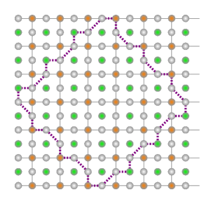
Figure 1: Distance-7 planar code. Data qubits are represented as grey circles, $X$ and $Z$-checks are represented as green and orange circles respectively.

Surface codes are a family of quantum error correcting codes in which the information of logical qubits is mapped to a set of physical qubits, commonly named as data qubits, which are displayed in a lattice array. Moreover, the measurement qubits that are used to measure the checks are also displayed within the lattice. Alexei Kitaev first proposed the concept of surface codes in his prominent work [40], where the qubits were displayed in a torus-shaped lattice. This toric code has periodic boundary conditions and it is able to protect two logical qubits. Nevertheless, such toric displacement of the qubits makes the hardware implementation and logical qubit connectivity complicated [83] since many experimental implementations such as superconducting hardware, for example, may require the system to be placed in a two-dimensional lattice. Thus, the so called planar code encoding a single logical qubit is obtained by stripping the periodic boundary conditions from the toric code [32, 84]. Specifically, it will be a $[[d^{2}+(d-1)^{2},1,d]]$ QECC. Furthermore, the number of data and measurement qubits used for protecting the single logical qubit can be lowered down, i.e. the rate of the code can be increased, by considering a specific set of data qubits and checks within the planar code. The obtained code is usually known as the rotated planar code, which will be a $[[d^{2},1,d]]$ [62]. FIG.1 shows a distance-7 planar code where the dashed lines indicate the subset of qubits that form the rotated planar code with the same distance. In this this tutorial we will consider the rotated planar code in a square lattice with Calderbank-Shor-Steane (CSS) structure due to its practicality and relevance at the time of writing. Note that this code is the one that has been recently implemented experimentally by Wallraff’s group at ETH Zurich [63] and by the Google Quantum AI team [64]. Nevertheless, the decoding methods discussed in this tutorial apply for all surface codes including the tailored versions proposed through the past years [41, 42, 87, 88] or the different lattices considered [62, 43, 89].

3.1 Stabilizer and check structure

Due to the structure of their stabilizers, CSS quantum surface codes have two types of checks: $X$-checks and $Z$-checks. The former detect $X$-errors, while the latter detect $Z$-errors. FIG. 2 portrays the structure of the check operators in a distance-5 CSS rotated planar code. As it can be seen in the figure, this structure fulfills the condition that the stabilizer generators form an abelian group [39]. The locality of the check operations ensures that checks that are far apart commute with each other, while adjacent checks commute either because they are of the same type and, thus, apply the same operators to their adjacent data qubits; or because they anti-commute for two data qubits at the same time, making the whole operators to commute. For example,

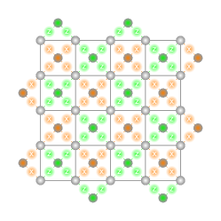
Figure 2: Distance-5 rotated planar code. The stabilizing operators that the checks yield over their adjacent data qubits are denoted through light green and orange circles.

$$\begin{split}M_{\mathrm{x}}M_{\mathrm{z}}\ket{\bar{\psi}}&=\mathrm{X}_{1}\mathrm{X}_{2}\mathrm{X}_{3}\mathrm{X}_{4}\mathrm{Z}_{3}\mathrm{Z}_{4}\mathrm{Z}_{5}\mathrm{Z}_{6}\ket{\bar{\psi}}\\ &=\mathrm{X}_{1}\mathrm{X}_{2}\mathrm{X}_{3}\mathrm{Z}_{3}\mathrm{X}_{4}\mathrm{Z}_{4}\mathrm{Z}_{5}\mathrm{Z}_{6}\ket{\bar{\psi}}\\ &=\mathrm{X}_{1}\mathrm{X}_{2}(-\mathrm{Z}_{3}\mathrm{X}_{3})(-\mathrm{Z}_{4}\mathrm{X}_{4})\mathrm{Z}_{5}\mathrm{Z}_{6}\ket{\bar{\psi}}\\ &=\mathrm{Z}_{3}\mathrm{Z}_{4}\mathrm{Z}_{5}\mathrm{Z}_{6}\mathrm{X}_{1}\mathrm{X}_{2}\mathrm{X}_{3}\mathrm{X}_{4}\ket{\bar{\psi}}\\ &=M_{\mathrm{z}}M_{\mathrm{x}}\ket{\bar{\psi}}=\ket{\bar{\psi}},\end{split}$$ (9)

where $M_{z}$ and $M_{x}$ are two arbitrary adjacent $X$ and $Z$-checks in the bulk of the code, respectively, and the data qubits labeled with $3$ and $4$ are located in between both checks.

The surface code is usually initialized by taking all the data qubits in the $\ket{0}$ state [63, 64]. Note that this corresponds to the logical $\ket{\bar{0}}$ state of the surface code and, thus, one can perform the desired computations over such logical state. As explained before, the data qubits of the surface code may undergo a Pauli error. The syndrome of the associated error is measuring the check operators, which correspond to the quantum circuits shown in FIG.3. The top circuit represents an $X$-check and the bottom circuit a $Z$-check. As seen in such figure, if an odd number of adjacent data qubits suffer from an $X$ or $Z$-error, the measurement of the respective $X$ or $Z$-checks will be triggered. However, as seen in the top image from FIG.3, in the event of an even number of errors, those will cancel, due to their unitary nature, and no error will be detected by the check operator measurement.

To sum up, whenever an error consisted of an odd number of $X$ or $Z$-errors affects the data qubits surrounding a check operator, the circuit from the picture will make said errors propagate to the measurement qubit associated to such check, changing the measurement and thus enunciating that an error has occurred in its vicinity [32].

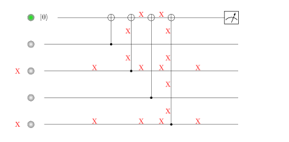
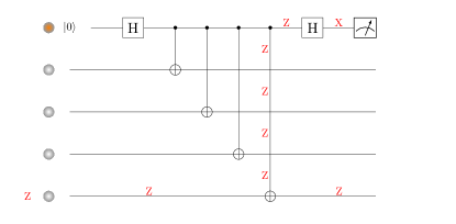
Figure 3: Stabilizing circuits of the $X$-checks (top) and the $Z$-checks (bottom). The green and yellow circles indicate the check qubits, and the grey qubits their 4 adjacent data qubits. In both cases an example of an error in the data qubits is introduced altogether with the path it follows within the circuit.

3.2 Types of errors and code threshold

In FIG.4 we show some examples of errors that may arise in the rotated planar code. In the upper right section of the code, there are three isolated Pauli errors, namely an $X$, a $Y$ and a $Z$-error, which cause the adjacent susceptible checks to exhibit non-trivial syndrome elements upon measurement. Note that the $Y$-error triggers both the $X$ and $Z$-checks that are adjacent to such data qubit. This happens because $Y$-errors are a combination of $X$ and $Z$-errors, neglecting the global phase, as seen in eq.(3). These isolated Pauli errors will be detected by the code, and using the syndrome information, the decoder will try to estimate which are those errors. Note that these errors have weight one, and since this specific rotated planar code has distance-$5$, those errors can be corrected.

In addition, two other errors forming a vertical and horizontal chain along the left and bottom boundaries are represented in FIG. 4. As seen in the figure, those error chains are not detected by the code since they do not trigger any of the surrounding measurement qubits. This is because each susceptible check is connected to two of the Pauli operators, i.e. it refers to the previously described case where there is an even number of operators acting on each of the checks. This error chains act non-trivially on the codestate without being part of the stabilizer group while presenting a trivial syndrome, i.e. they belong to the normalizer of the code. This type of errors receive the name of logical errors [32]. Specifically, the left error chain is a logical $Z$-error, $\mathrm{Z}_{L}$, the bottom error chain is a logical $X$-error, $\mathrm{X}_{L}$, and the combination of them two is a logical $Y$-error, $\mathrm{Y}_{L}$. Notice that the anti-commutation relation $\mathrm{X}_{L}\mathrm{Z}_{L}=-\mathrm{Z}_{L}\mathrm{X}_{L}$ is preserved through the bottom left data qubit. Note that these are just two examples of logical errors, there are other possible logical operators. Moreover, if a logical error is applied, the resulting state will still be within the codespace, so eq.(4) will still be preserved for the new sate and it will remain invariant upon the application of stabilizer operators. This can be reflected in the bottom right of FIG.4, where the application of the bottom left $Z$-check modifies the shape of the $\mathrm{X}_{L}$ operator while still commuting with all the checks.

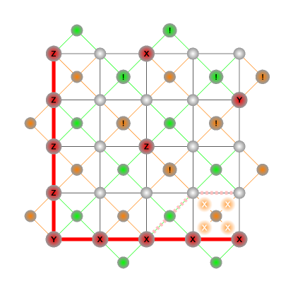
Figure 4: The figure shows a CSS rotated planar code, with physical Pauli operators represented by red circles. Check measurements resulting in non-trivial syndrome elements are marked with an exclamation mark. The thick red line represent the shape of two logical operators, while the pink dashed line shows the changed path of one of them after interacting with a stabilizer.

When protecting against quantum noise, experiencing a logical error is fatal since those alter the information stored in the code without any indication from the checks and, thus, cannot be detected nor corrected. One way of mitigating the impact of logical errors is to increase the size of the surface code. By doing so, the code distance increases and, therefore, the minimum number of Pauli operators needed to form a logical error will also be higher, making such event to be more improbable. This comes from the fact that logical errors belong to the normalizer of the code and the distance is defined as the minimum weight of those Pauli operators. Although it may seem intuitive that a larger surface code would perform better, this is not always the case. The momentous result in quantum computing named the threshold theorem states that the performance of a QECC improves as its distance increases, provided that the physical error rate of the data qubits is below a certain value [29, 40, 90, 91]. This value is known as the probability threshold ($p_{th}$). As long as the physical error rate is below $p_{th}$, increasing the size of the surface code will lead to a better code performance.

The probability threshold is a useful metric for benchmarking the performance of the surface code under a particular decoder. However, the value of the threshold does not only depend on the code and decoder in consideration but also on the structure of the underlying noise that affects the physical qubits of the code. In the following section, we will discuss the origin of quantum noise and the most relevant noise models considered in QEC.

4 Noise models

The main obstacle to construct quantum computers is the proneness of quantum information to suffer from errors. There are many error sources that corrupt quantum information while being processed such as state preparation and measurement (SPAM) errors or errors introduced by imperfect implementations of quantum gates, for example. Many of the errors occur due to the fact that the technology used for manipulating qubits is imperfect [32, 33]. However, qubits do also suffer from errors due to their undesired and unavoidable, in principle, interaction with their surrounding environment. This last source of errors is named as environmental decoherence, and corrupts quantum information even if the quantum system is left to evolve freely [20, 34, 30, 35]. Thus, decoherence poses a fundamental problem to the field of quantum information processing since its existence does not depend on imperfect implementations of qubit manipulations or measurements, which we may deem as engineering problems. Therefore, quantum error correction will be necessary if we want to run arbitrarily large quantum algorithms with enough precision so that the obtained results are reliable, even if perfect quantum gates, measurements and state preparations are available.

4.1 Decoherence

In general, decoherence comprises several physical processes that describe the qubit environment interaction, and the nature of those processes depends on the qubit technology, i.e. superconducting qubits, ion traps or NV centers, for example. However, most of those physical interactions can be grouped into three main decoherence mechanisms since their operational effect on the two-level coherent system that is the qubit is the same [30, 92]:

• Energy relaxation or dissipation: this mechanism includes the physical processes in which a quantum mechanical system suffers from spontaneous energy losses. For example, atoms in excited states tend to return to the ground state by spontaneous photon emission. The amalgamation of relaxation processes is described by the so called relaxation time, $T_{1}$, which is the characteristic timescale of the decay process [30, 35, 92].

• Pure dephasing: these physical processes involve the corruption of quantum information without energy loss. For example, this occurs a photon scatters in a random manner when going through a waveguide. Pure dephasing is also quantified by the characteristic timescale of the decay process [35, 92], which in this case is named as pure dephasing time, $T_{\phi}$.

• Thermal excitation: this refers to the undesired excitation of the qubit from the ground state to the excited state and the assisted relaxation from the excited state to the ground state caused by the finite temperature of the system [20, 92, 93]. Every qubit platform will be at a finite temperature in the real world, but the contribution of thermal excitation can be usually neglected when qubits are cooled down significantly. Generally, the temperature of the system, $T$, and the energy levels of the ground state and the excited state quantify this effect on the quantum system.

There are many ways in which this set of physical interactions can be mathematically described such as the Gorini-Kossakowski-Lindblad-Sudarshan (GKLS) master equation [94, 95, 96] or the quantum channel formulation [30, 97]. In the context of QECC, quantum channels are used to describe noisy evolution. In general, quantum channels are linear, completely-positive, trace-preserving (CPTP) maps between spaces of operators. As a consequence of those properties, quantum channels fulfill the Choi-Kraus theorem, implying that the application of such maps on a density operator $\rho$ can be written as the following decomposition [20, 30, 97]:

$$\mathcal{N}(\rho)=\sum_{k}E_{k}\rho E_{k}^{\dagger},$$ (10)

where the $E_{k}$ matrices are named Kraus or error operators, and should fulfill $\sum_{k}E_{k}^{\dagger}E_{k}=\mathrm{I}$ since the quantum channels must be trace-preserving. Thus, quantum channels are characterized by sets of Kraus operators that are associated to some physical interaction of the qubit with its surrounding environment.

The generalized amplitude and phase damping channel (GAPD), $\mathcal{N}_{\mathrm{GAPD}}$, describes the evolution of a quantum state when decoherence arises from the three qubit-to-environment interactions presented before [30, 35, 93, 98, 99]. Such channel consists of a generalized amplitude damping channel (GAD) describing the thermal and relaxation interaction [93, 98, 99] and of a pure dephasing channel (PD) [30, 35]. The action of the GAD is described by the damping parameter, $\gamma$, and the probability that the ground state is excited by finite temperature, $N$. The damping parameter relates to the relaxation time of the qubit as, $\gamma(t)=1-e^{-(2n_{\mathrm{th}}+1)t/T_{1}}$, with $t$ being the evolution time, while $n_{\mathrm{th}}$ and $N(n_{\mathrm{th}})$ depend on the temperature and the energy gap of the system [93, 98, 99]. Whenever the thermal excitation is considered negligible, $n_{\mathrm{th}}\approx 0$ and $N(n_{\mathrm{th}})=0$; and such channel reduces to an amplitude damping channel (AD). The pure dephasing channel (PD) is described by the so called scattering probability, $\lambda$, which relates to the pure dephasing time as, $\lambda(t)=1-e^{-2t/T_{\phi}}$, with $t$ the evolution time again [35, 78]. In this sense, the GAPD channel is defined by those parameters.

4.2 Twirled quantum channels

Therefore, the GAPD channel is a complete mathematical description of the evolution that a qubit undergoes when decoherence is considered. The problem with this quantum channel is the fact that it is not possible to simulate it efficiently by means of classical computer as the dimension of the Hilbert state increases exponentially with the number of qubits considered [30]. This makes it impossible to construct and simulate efficient error correction codes that will be used for protecting quantum information by using conventional methods. That is why a technique named twirling is usually employed in order to obtain channels that can be managed by classical computers and that capture the essence of the GAPD channel [30, 35, 100, 101]. The significance of the twirling method comes after the fact that a correctable code for the twirled channel will also be a correctable code for the original channel [30, 102] and, thus, we can consider the simplified channels for designing codes that will eventually be successful for the actual noise. Following this logic, the most common twirling operations are the so called Pauli [30, 100, 78] and Clifford twirl approximations [30, 35, 101, 78] (PTA and CTA), where the quantum channel in consideration is averaged uniformly with the elements of the Pauli group, $\mathcal{P}$, and the elements of the Clifford group, $\mathcal{C}$, respectively. Twirling the GAPD channel with these two groups results in Pauli channels, i.e. those with Kraus operators $\{\sqrt{(1-p_{x}-p_{y}-p_{z})}\mathrm{I},\sqrt{p_{x}}\mathrm{X},\sqrt{p_{y}}\mathrm{Y},\sqrt{p_{z}}\mathrm{Z}\}$ with probabilities:

• Pauli twirl: $p_{x}=p_{y}=\frac{\gamma}{4}$ and $p_{z}=\frac{2-\gamma-2\sqrt{1-\gamma-(1-\gamma)\lambda}}{4}$.

• Clifford twirl: depolarizing channel, $p_{x}=p_{y}=p_{z}=\frac{2+\gamma-2\sqrt{1-\gamma-(1-\gamma)\lambda}}{12}$.

The usefulness of Pauli channels resides in the fact that they can be efficiently simulated in classical computers since they fulfill the Gottesman-Knill theorem [20, 103]. Thus, we can use them in order to construct and simulate quantum error correction codes that will then be useful to protect qubits from the more general GAPD (or APD) noise [30]. Note that the CTA results in a depolarizing or symmetric Pauli channel where all the errors are equiprobable, while the PTA presents a probability bias respect to the $\mathrm{Z}$ types of errors. Therefore, the PTA is usually referred as the biased noise model, where the bias is defined as $\eta=p_{z}/(p_{x}+p_{y})\approx T_{1}/T_{2}-1/2$ [104]. The bias of the channel varies significantly as a function of the technology or even as a function of the qubit of a processor being considered [30].

4.3 Noise models for multiple qubits

There are several ways in order to construct the $n$-qubit quantum channel that is required to study the action of the quantum error correction code being designed [30, 104, 105]. The literature on QEC usually assumes that each of the qubits of the system experience noise independently. In this sense, the following $n$-qubit twirl approximation channels will be considered:

• Independent and identically distributed (i.i.d.): in this model each of the qubits will have the same experience of suffering a particular Pauli error [30]. Joining this with the fact that the noise is considered to be independent, the probability that a particular $n$-qubit Pauli error, $\mathrm{A}=\mathrm{A}_{1}\otimes\mathrm{A}_{2}\otimes\dots\otimes\mathrm{A}_{n}$ with $\mathrm{A}_{j}\in{\{\mathrm{I,X,Y,Z}\}}$, will be given by

  $$p_{\mathrm{A}}(\mu_{T_{1}},\mu_{T_{2}})=\prod_{j=1}^{n}p_{\mathrm{A}_{j}}(\mu_{T_{1}},\mu_{T_{2}}),$$ (11)

  where $p_{\mathrm{A}_{j}}$ is described by the PTA (biased) or CTA (depolarizing) approximations given before, and where $\mu_{T_{1}}$ and $\mu_{T_{2}}$ refer to the mean values of the relaxation and dephasing times. Taking the mean value is the usual approach.

• Independent and non-identically distributed (i.ni.d.): in this model every qubit experiences a different probability of suffering a Pauli error [104, 106]. The motivation of this error model is the fact that state-of-the-art quantum processors are consisted of qubits whose relaxation and dephasing times differ significantly. Considering that the environment-to-qubit interaction is still independent from qubit-to-qubit, the probability of occurrence for a $n$-qubit Pauli error is given by

  $$p_{\mathrm{A}}(\{T_{1}^{j}\}_{j=1}^{n},\{T_{2}^{j}\}_{j=1}^{n})=\prod_{j=1}^{n}p_{\mathrm{A}_{j}}(T_{1}^{j},T_{2}^{j}),$$ (12)

  where $p_{\mathrm{A}_{j}}(T_{1}^{j},T_{2}^{j})$ is again given by the PTA (biased) and CTA (depolarizing) approximations, but now each of the terms have particular values of relaxation and dephasing times.

4.4 SPAM and gate errors

As stated before, physical qubits experience errors from sources other than the unavoidable decoherence. Those errors refer to imperfect implementation of the operations that are done whenever the physical qubits are prepared, measured or manipulated by means of quantum gates, and are usually referred as circuit-level noise [20, 43, 107]. These errors are usually classified and modelled in the following way:

• SPAM errors: these refer to the errors that occur due to the imperfect preparation of the states that are needed to initialize the surface code and the fact that the measurement operations done to detect the syndrome are not always successful. Since it is usually considered that a surface code is initialized with all the physical qubits on the $\ket{0}$ state, state preparation errors are usually modelled so that a $\ket{1}$ state is prepared instead of the $\ket{0}$ with a probability of error $2p_{\mathrm{prep}}/3$ [32, 43, 107]. This is the same as considering a depolarizing channel after state preparation. Imperfect measurements are usually modelled by considering that the single-qubit measurement is flipped with a probability $2p_{\mathrm{meas}}/3$ error [32, 43, 107].

• Noisy single-qubit gates: due to their imperfect implementation, single qubit quantum gates, $\mathcal{U}$, do not perform the desired operation in a perfect way and, thus, introduce noise to the qubit. In this sense, the noisy quantum gate, $\mathcal{\tilde{U}}$, can be seen as the operation of the quantum gate followed by a quantum channel, $\Lambda$, that describes the noise introduced by the gate, i.e. $\mathcal{\tilde{U}}=\Lambda\circ\mathcal{U}$ [20, 74, 108]. In this sense, single-qubit gate errors are usually modelled by considering that they are followed by a depolarizing channel with probability of error $p_{\mathrm{1Q}}$ [32, 43, 107]. This implies that an $\mathrm{X}$, $\mathrm{Y}$ or $\mathrm{Z}$-error will be applied to the physical qubit with probability $p_{\mathrm{1Q}}/3$.

• Noisy two-qubit gates: similar to the single-qubit gate, two-qubit gates are also modelled by a noisy channel being applied after the perfect operation. However, the usually considered error map is the two-qubit depolarizing channel with probability of error $p_{\mathrm{2Q}}$ [32, 43, 107]. Therefore, a Pauli error of the set $\{\mathrm{I,X,Y,Z}\}^{\otimes 2}\setminus\mathrm{I}^{\otimes 2}$ will be randomly applied after the perfect two-qubit gate with probability $p_{\mathrm{2Q}}/15$.

It is important to state that a biased circuit-level noise model can also be considered if the depolarizing channels are changed by Pauli channels with a bias towards $\mathrm{Z}$-errors equal to $\eta$ [107].

4.5 Erasure errors

To finish with this section, we will discuss another error type that can corrupt the qubits of a quantum computer, named erasure error, and that will be considered for the Union Find decoder [109, 110]. Erasure errors come from two types of physical mechanisms that qubits may experience:

• Leakage: qubits are defined as two-level coherent systems. However, when physically implemented, there exist other levels that can be populated. This would imply that the qubit has left the computational subspace and, thus, it is not useful anymore [109, 111]. Leakage may arise due to decoherence processes that make the qubit to leave the computational space or due to leaky quantum gates.

• Loss: this refers to the scenario where the qubit is physically missing [109, 112]. For example, in a photonic system the qubit encoded in a photon may be lost.

In this context, an erasure channel describes the fact that a qubit at a known location has been lost with probability $p_{e}$ [110]. The fact that it is known which of the qubits is lost is important since it provides with useful information for treating those errors. The detection of leakage events in physical qubits can be done by means of the quantum jump technique or by means of ancillary qubits, for example [110, 111, 113, 114, 115]. Errors of this type with unknown locations are named deletion errors in the literature [116]. The significant difference between deletion and erasure errors lies in the fact that a deletion error leads to a decrease in the number of qubits of the system, i.e. the qubit is effectively lost, while an erasure error occurrence does not decrease the number of qubits. In this sense, the erasure channel on a qubit, $\rho$, may be described as

$$\mathcal{N}_{\mathrm{er}}(\rho)=(1-p_{e})\rho+p_{e}|e\rangle\langle e|,$$ (13)

where $|e\rangle$ refers to an erasure flag giving the information that such qubit has been erased. Since erasure errors are detected and their location is known, qubits subjected to such errors can be reinitialized, which results in those being subjected to a random Pauli error after the measurement of the stabilizers is performed [109].

5 Decoders for the surface code

As described in the previous sections, surface codes have the ability of detecting errors experienced by the data qubits, which can be accurately modelled by elements of the Pauli group $\mathcal{G}_{n}$. However, once the error syndrome is measured, an estimation of the channel error must be done using such information, $\hat{E}(\bar{s})$, so that active error correction can be performed on the noisy qubits. The methods used for performing this inference of the error are named decoders. Once the decoder makes a guess of the channel error, the recovery operation is performed by applying $\hat{E}^{\dagger}(\bar{s})$ since the elements of the Pauli group are unitary matrices.

Therefore, decoding methods for error correction codes are a critical element of the code itself since their efficiency on making correct guesses of channel error will be what will determine if the method is successful or not. In this sense, the threshold of a code is a function of the decoder in question, i.e. the code can perform better or worse as a function of the method used. Making the decoder to be more accurate usually comes with the drawback of increasing its computational complexity, which ultimately makes it to be slower in making guesses. Decoders must be fast enough since the action of decoherence will not stop while estimating the error after measurement, implying that the qubit may suffer from additional errors to which the decoder will be oblivious. Thus, a slow decoder will ultimately have a bad performance (See appendix LABEL:appBack) for more details on why real time decoding is required). To sum up, the trade-off between the accuracy and complexity of the methods is vital for the field of quantum error correction [56, 57].

Surface codes can be decoded by using many methods [32, 117, 118, 119, 120, 109, 121, 46, 122, 123, 124, 125]. In this section we will explain the operation and performance, in terms of correction ability and complexity, of the main decoders for surface codes: the minimum-weight perfect matching [32, 117, 118, 119, 120], the Union-Find decoder [109], the Belief Propagation decoder [54, 46, 122] and the Tensor Network or Matrix Product State decoder [121]. In addition, we will also discuss variants of those decoding methods that have proven to be more efficient in terms of error correction ability or complexity as the Belif-Propagation Ordered Statistics Decoder (BPOSD) [46, 122], for example. Furthermore, we discuss other decoding algorithms in the literature that can be used for decoding the surface code. Many of those were proposed for decoding other topological codes such as the toric or color codes, but could, in principle, be applied for the rotated planar code. Specifically, we discuss Cellular-automaton [124], renormalization group [123], neural network or machine learning based [125] and MaxSAT [126] decoders. The end of the section includes an overview of the available software implementations available to the general public of all those decoding methods.

5.1 The Minimum Weight Perfect Matching Decoder

Before the operation of the MWPM decoder is described, some definitions of graph theory must be provided [127]. Consider a weighted graph $G$ composed by ($V$,$E$,$W$), where $V=\{v_{i}\}$ are the vertices, $E=\{e_{ij}\}$ is the set of edges which satisfy $i\neq j$ and $e_{ij}=\{v_{i},v_{j}\}$, meaning that the edge $e_{ij}$ connects the nodes $v_{i}$ and $v_{j}$, and $W=\{w_{e}\}$, $e\in E$, which is the set of weights attributed to each edge. A matching of graph $G$ is a subset of edges, denoted as $M\subseteq E$, such that for any two edges $e$ and $f$ in $M$, $e$ and $f$ do not share any common vertices. In other words, $M$ is a set of edges without common endpoints. A perfect matching is a matching that additionally satisfies the condition that every vertex in $V$ is incident to exactly one edge in $M$. A minimum weight perfect matching is the perfect matching with the smallest possible weight among all possible perfect matchings [117, 127], where the weight of a matching is defined as the sum of the weights of its edges: $\sum_{e\in M}w_{e}$. Additionally, a complete graph is a graph with the property that $\forall v_{i},v_{j}\in V,i\neq j,\exists e_{ij}\in E$.

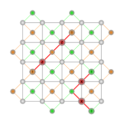
Figure 5: Graphical representation of the effect of a Pauli error in a 5x5 rotated surface code. The red lines connecting non-trivial checks represent chains.

As explained before, when the data qubits of the surface code experience a Pauli error, the checks adjacent to an odd number of errors turn into non-trivial syndrome elements. On the other hand, checks adjacent to an even number of errors will not be triggered by them, since the product of two errors of the same type will cancel. Therefore, combinations of those two types of events can be viewed as error chains over the lattice of data qubits that terminate in non-trivial checks. An example of these events is shown in FIG.5. In this sense, due to the CSS structure of the surface codes considered, two separate subgraphs where the nodes represent the non-trivial syndrome elements can be constructed: one for the $X$-checks and one for the $Z$-checks. The aforementioned nodes must be connected with all the other nodes resulting in complete subgraphs, each edge connecting two nodes must be of weight equivalent to the minimum distance between the respective checks in terms of data qubits. Once the two complete subgraphs are obtained, a perfect matching with minimum weight is seeked on those subgraphs so that the error chains corrupting the data qubits may be identified [32, 127]. One condition in order to construct a graph in which a minimum weight perfect matching can be found is that that all correctable error chains within the code have two non-trivial endpoint checks [127]. Nevertheless, the data qubits on the boundary of the code are not covered through four checks and so they can derive in chains with only one endpoint. Thus, it is necessary to consider virtual checks adjacent to the aforementioned boundary data qubits. Specifically, each non-trivial syndrome will have an associated virtual check outside the boundary of the code. Those virtual check nodes will also be connected among the other virtual checks, but the weight of those edges will be considered to be zero [127].

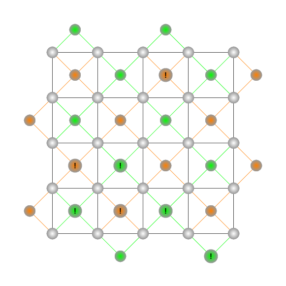
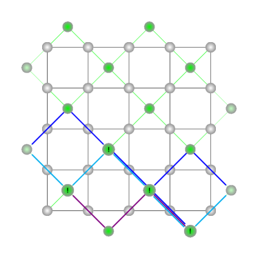
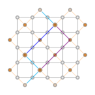
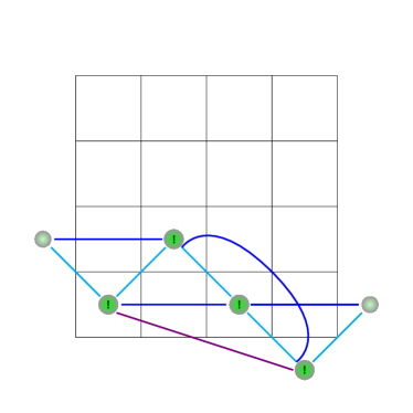
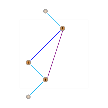
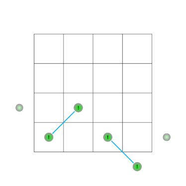
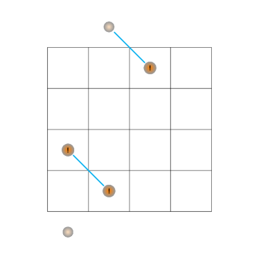
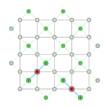
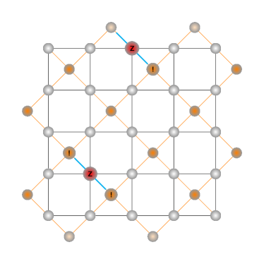
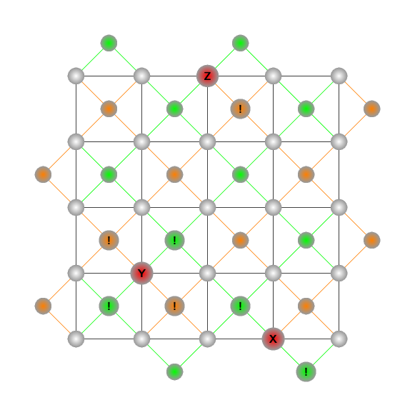
Figure 6: Graphical representation of a MWPM process for a specific syndrome in a 5x5 surface code.

In FIG. 6, we provide an example of the operation of the MWPM decoder for a specific detected error pattern syndrome. From top to bottom and then from the left column to the right column, the first row shows the considered syndrome, where the exclamation marks correspond to the checks that have measured a non-trivial syndrome element. The second row depicts two separate graphs, one consisting of all $X$-checks (green nodes) and the other of all $Z$-checks (orange nodes). Note that in both graphs, the previously discussed virtual checks are located in the boundaries: on the left and right boundaries for the $X$-checks and on the top and bottom for the $Z$-checks. The data qubits of the code are then considered to be the edges of such graphs connecting the checks nodes with their nearest ones. Over these graphs, all the shortest paths connecting all non-trivial checks with each other and with their nearest virtual qubit are considered for the matching problem. These paths are represented with cyan, blue and violet colors for paths of weights $1$, $2$ or $3$ respectively. By means of those paths, the subgraphs shown in the third row are constructed, where the weights of the edges are given by the number of data qubits that are crossed when following the path from non-trivial check to non-trivial check, i.e. each of the edges of the graphs of the second row of the figure has weight 1. Then, in the right column, the minimum weight perfect matching of those subgraphs is computed. The result of said process can be seen in the first row, notice how virtual qubits can be left unmatched. The matchings of each of the subgraphs refer to $X$ or $Z$-operators applied to the data qubits that the matching crosses. Thus, for the example in consideration, the second row of the right columns presents the operators that will be applied on the data qubits of the surface code. The $X$-checks recover $X$-errors and the $Z$-checks recover $Z$-errors. In the last row of the figure, we present the final recovery operator, where it can be seen that whenever an $X$ and $Z$-error are estimated from each of the graphs for the same data qubit, the resulting recovery operation is a $Y$-operator.

The MWPM decoder estimates the Pauli error with minimum $X$ and $Z$ weight (since it considers said errors independently) that corresponds to a given syndrome. In this sense, this decoder always outputs an error whose syndrome is the same as the one measured. In addition to always matching the syndrome, if it succeeds in matching the endpoints of an error chain to the observed syndrome it will always yield the correct outcome, even if the recovered error differs from the input one. The reason for this to happen is that the elements of the stabilizer in a 2D surface code correspond to Pauli sequences that form a closed loop in the surface code [32, 104, 129]. Thus, if the estimated error forms a closed chain with the true error occurred on the surface code, the resulting Pauli element will belong to the stabilizer set of the code and, thus, the correction will have been successful (recall eq.(6) and degeneracy of errors). In FIG. 7, we pictorically present this scenario where two error chains with same endpoints are separated by a stabilizer element. Note also that whenever an error that forms an error chain that is a loop on the data qubits of the code, all the checks will have trivial values but the codestate will not be affected by it as it will be a stabilizer element. Thus, those types of chains will be non-detectable but unharmful for the code.

5.1.1 Complexity

As described before, the most critical part of the MWPM decoder consists in finding the perfect matching with minimum weight once the subgraphs are constructed from the syndrome information. An algorithm to efficiently solve such computational problem was proposed by Jack Edmonds back in the 60s, the so called Blossom’s algorithm [117]. In general, the MWPM decoder is dominated by the Blossom step of the algorithm whose worst-case complexity in the number of nodes $N$ is $O(N^{3}\log{(N)})$ [57, 120]. However, the expected runtime of the decoder is roughly $O(N^{2})$ whenever the decoder is implemented such that all Dijktra searches are needed for computing the subgraphs where the matching of interest is needed [120, 57]. Therefore, and due to the importance speed for real-time decoding, several implementations of the MWPM decoder have been proposed such as Fowler’s implementation with $O(1)$ parallel expected runtime [127] or the more recent Sparse Blossom by Higgot and Gidney with an observed complexity of $O(N^{1.32})$ [57] and Fusion Blossom by Wu with $O(N)$, i.e. linear complexity [118, 119, 130]. Each of the implementations have their own advantages and disadvantages, as for example, Sparse Blossom has a faster single-thread performance than Fusion Blossom, but the latter supports multi-thread execution, implying that it can be faster than the former if enough cores are available [57]. Proposing faster MWPM implementations is an arduous but significant task, since large distances are precised in order to have a fault-tolerant quantum computer, and the decoding schemes also need to be scalable in the sense that they are fast enough when the distance of the code increases.

Following the previous discussions, it can be seen that the MWPM decoder follows the QMLD decoding rule as it aims to estimate the most probable error for the given syndrome. Note that, here, finding a perfect matching with minimum weight in the subgraphs formed with the measured syndrome implies that the Pauli element estimated will be the most probable to occur considering pure $X$ and $Z$ noise . Applying the suboptimal decoding rule has been observed to be an efficient for low physical error probabilities [120].

5.1.2 Performance and threshold

In FIG. 8 we plot the performance of the rotated planar code in terms of the logical error probability ($P_{L}$), that is, the probability of the decoding process failing in predicting an error given its syndrome, as a function of the physical error probability ($p=p_{x}+p_{y}+p_{z}$) whenever it is decoded using a MWPM decoder. Two noise models are considered: the top figure considers an i.i.d. depolarizing error model ($p_{x}=p_{y}=p_{z}$), while in the bottom figure considers an i.i.d. biased Pauli channel with bias $\eta=100$. The results show how the MWPM decoder performs better when considering noise channels closer to the depolarizing channel. Specifically, not only the logical error probabilities are significantly higher for the biased case when a physical error probability is fixed, but also the probability threshold $p_{th}$ is lower. This performance decrease when the channel is biased can be explained by the fact that both subgraphs are considered independently. Considering a bias towards $Z$-noise results in the $Z$-subgraph correspondent to the $Z$-checks being more dense, i.e. more non-trivial syndromes are triggered, as opposed to the $X$-checks one. This results in the $Z$-subgraph reaching the probability threshold before the total physical error probability reaches the threshold of the depolarizing channel. Further increasing the bias of the channel will produce a decrease of the $p_{th}$ until the extreme value of $\eta\rightarrow\infty$, that is, a pure dephasing error model. At such point, all triggered syndromes will correspond to the same subgraph, i.e., the right column in FIG. 6. Table 1, shows some $p_{th}$ for different biases when decoded using the standard MWPM decoder for the rotated planar code.

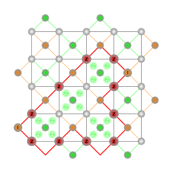
Figure 7: Two $Z$-error chains that share the same endpoints and the stabilizing operator checks which separate them.

5.1.3 Modifications and re-weighting for specific noise models

Biased channels are important since experimentally implemented qubits have shown lower dephasing times, $T_{2}$, than relaxation times, $T_{1}$, which implies that those qubits are more prone to suffer from dephasing errors than bit-flip errors (recall the GAPDPTA channel) [30, 35, 104]. Bias values in the range of $\eta\in[1,10^{6}]$ are typical depending on the technology used for constructing the qubits [30, 78]. Therefore, the way to deal with biased noise has been studied by modifying the surface code structure so that the $Z$-subgraph contains more information than the $X$-subgrahp, i.e. rectangular surface codes, [41, 87, 131] or by modifying the MWPM decoder by making it aware of the symmetries of the code [132]. In addition, the noise in experimentally constructed hardware is not identically distributed (recall the i.ni.d. error model) [88, 104, 133, 106]. The performance of surface codes is significantly affected by such non-uniformity of the noise in the data qubits of the lattice, as some of the data qubits will have a higher tendency to suffer from errors than other, and the standard MWPM decoder calculates the perfect matching considering that all the qubits are equiprobable. Thus, methods based on reweighting the syndrome subgraphs as a function of the probability of error of each of the qubits have been proposed so that the MWPM problem is solved over a weighted graph that takes such effects in consideration [88, 104]. Another limitation of the standard MWPM decoder is the fact that since the $Z$ and $X$-subgraphs are decoded independently, $Y$-errors are underestimated. In fact, since $Y$-errors are combinations of bit- and phase-flips, it can be considered that there exists a correlation among them. Therefore, information can be passed from the $Z$-subgraph to the $X$-subgraph, and vice versa, so that the correlation betwen those events is taken into account by reweighting the other subgraph as a function of what has been estimated in the other [88, 134, 135].

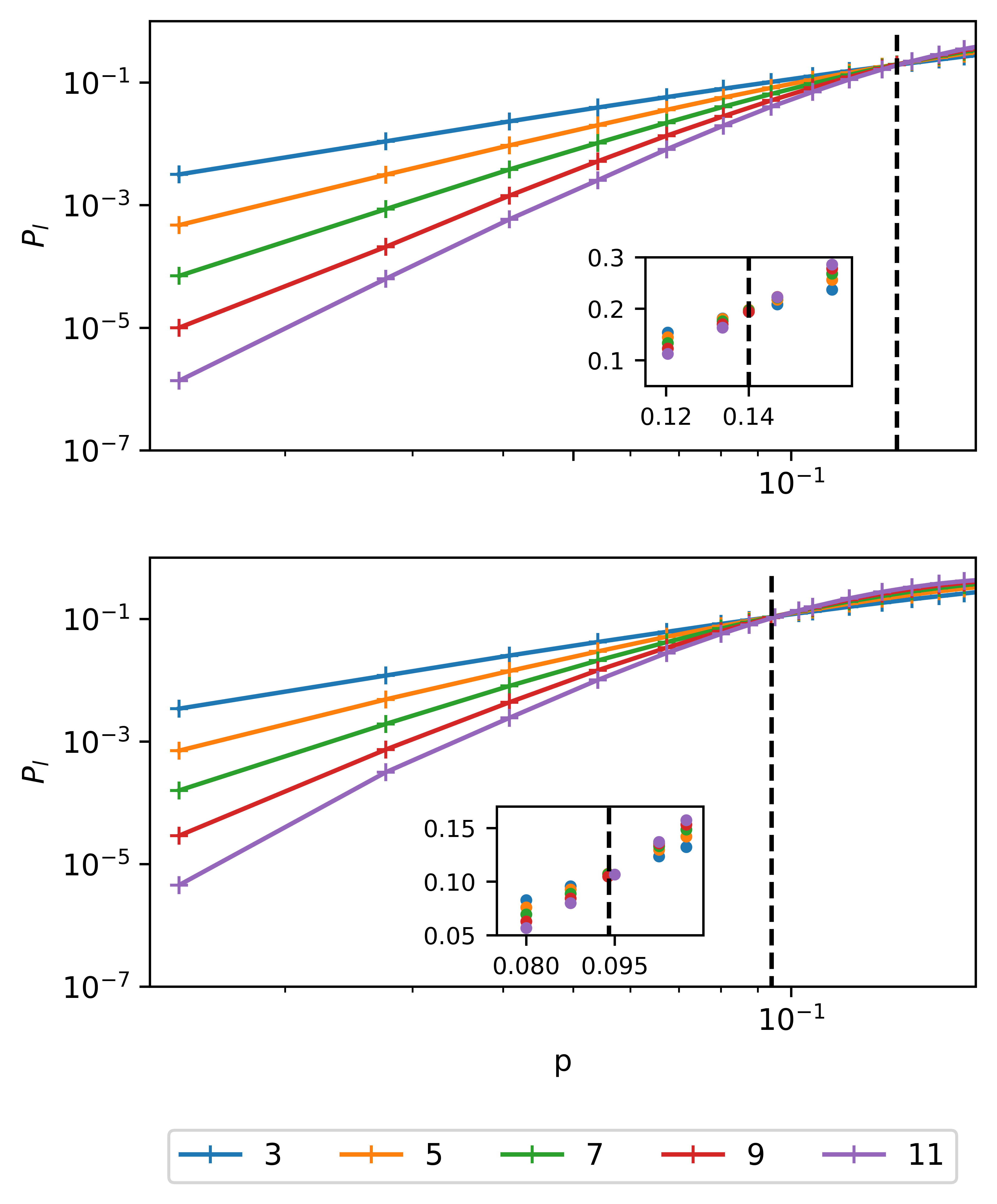
Figure 8: Logical error probability with dependence on the physical error probability under depolarizing (top) $\eta=100$ (bottom) noise. The dashed line represents the $p_{th}$ case and the subplots are close ups to the points near the $p_{th}$.

5.1.4 Measurement errors

Another important thing to consider when decoding surface codes is the fact that the measured syndromes might be erroneous [32, 87, 107]. This means that the measured syndrome does not correspond to the Pauli operator affecting the data qubits after measurement. This may come due to the fact that the measurement operations are not perfect (recall SPAM errors) or due to the so called error propagation. Error propagation refers to the fact that Pauli errors on one qubit can propagate to other qubit when performing a two-qubit gate. For example, if we have an $X$-operator in the control qubit of a $\mathrm{CNOT}$ gate, such operator propagates to the target qubit, i.e. $\mathrm{CNOT}(\mathrm{X}\otimes\mathrm{I})=\mathrm{X}\otimes\mathrm{X}$. As a consequence of this, the circuit-level noise coming from the measurement qubits can propagate to the data qubits, changing the Pauli error due to propagation and, thus, making the measured error to be imperfect even with perfect SPAM. Those erroneous measurements have a big impact in code performance, lowering the code threshold in significant manner when circuit-level noise is considered [32, 87, 107, 136]. In order to deal with this problem, several measurement rounds are done before decoding so that a space-time like graph is obtained in which the MWPM problem is performed to estimate the error. Usually, $d$ measurements are recorded for a distance-$d$ surface code [32, 136]. It is noteworthy to say that once the measurements are done, a non-trivial syndrome element for a measurement that follows another one will be a measurement that has flipped from such last round, refer to the Appendix B for a more detailed description. Then, the complete graph is constructed by connecting all those non-trivial elements both spatially and temporally. This consideration enlarges the size of the graph where the perfect matching with minimum weight must be computed and, therefore, the complexity of the algorithm increases considerably. By considering this space-time decoding, the performance of the code will improve when compared to single-round decoding, but the code threshold significantly decreases compared to the perfect measurement scenario [32, 87, 107].

$\eta$	$p_{th}$
1/2	0.140
1	0.138
10	0.098
100	0.095
1000	0.088

Table 1: Probability threshold values for different biases in the rotated planar code under the MWPM decoding scheme.

5.2 Union-Find decoder

The Union-Find decoder (UF) is a decoding scheme proposed by Nicolas Delfosse and Naomi Nickerson in 2017 which also consists in mapping the syndrome into a graph problem [109]. However, this decoder is based on clustering the non-trivial syndrome elements of the subgraphs by considering that Pauli errors at a known location can be treated as erasure errors. As mentioned in the error model section, an erasure error within a physical qubit can be treated as the qubit itself being in a mixed state (subjected to a random Pauli error). Therefore, having a uniform probability distribution for $I$-, $X$-, $Y$- or $Z$-operators [53] and, most importantly, a known location. Thus, for a pure erasure error model, all the qubits undergoing said erasure errors are localized. The surface code under the erasure channel can be efficiently decoded in linear time, through a method named peeling decoding scheme [137]. In light of this, the UF decoder is based on the idea of transforming the decoding problem of a surface code experiencing Pauli noise into an erasure error decoding problem. By doing this, the UF decoder achieves a decoding complexity of almost linear time $O(n\alpha(n))$ [109], where $\alpha$ is the inverse of the Ackerman function and for all practical purposes $\alpha(n)\leq 3$ [138]. In order to do so, the UF decoding process consists of two different steps: syndrome validation and erasure decoder. The syndrome validation step consists on mapping the set of Pauli errors or a mixture of Pauli and erasure errors into clusters of overall erasure errors [109]. Note that mixtures of Pauli and erasure errors can be considered by the UF decoder since the idea is to only have erasure errors. Once the step is completed, the erasure decoder is based on the peeling decoder [137].

5.2.1 Syndrome validation

Similar to the MWPM decoder, the UF decoder works on two separate graphs, one for the $X$-checks and one for the $Z$-checks, and they include the boundary virtual checks discussed before. In the syndrome validation step, the checks within each of the graphs are considered to be even parity nodes if they correspond to a trivial measured syndrome element and odd parity nodes otherwise [109]. All odd parity nodes are considered clusters (at the beginning every cluster will have just one element). Then, every cluster will grow, encompassing its nearest check neighbours. When a cluster grows, its parity is updated to the one of the combined constituent checks. Checks with zero parity will contribute trivially to the overall parity of the cluster. When two different clusters come into contact, they merge into a single cluster the parity of which is the resulting one of combining the two previous ones. A cluster is frozen, i.e. it stops to grow if:

• The updated parity of the cluster results in an even parity.

• The cluster reaches a virtual qubit.

• The growing cluster merges with another cluster that is frozen as a result of reaching a virtual qubit.

FIG. 9 presents an example of syndrome validation for the $X$-check graph (note that the execution of the Z-check graph will be performed in the same manner). The top figure represents the error considered and the triggered checks. Note that we omit the $Z$-checks which we represent with orange circles for simplicity. On the second picture from the top, the clusters increase reaching the adjacent checks from the adjacent data qubits from the initial non-trivial checks. The leftmost and rightmost non-trivial checks reach the boundary and, thus, freeze, as shown in the third row. We depict frozen clusters with the cyan color. Moreover, the two triggered checks on the bottom right of the surface code also freeze as a result of the even parity of the cluster. Therefore, by the third figure, only one cluster will continue to grow. For that reason, as it can be seen in the fourth figure, the cluster grows again making contact with one of the leftmost frozen clusters. Consequently, they merge into a single cluster which is frozen because the new cluster has reached a virtual qubit. This makes the syndrome validation step to conclude, as it can be seen in the last row of FIG. 9.

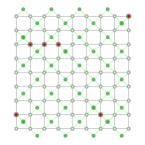
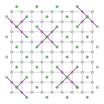
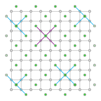
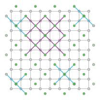
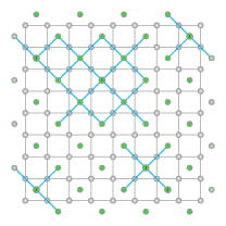
Figure 9: Graphical representation of the cluster growth in a distance-9 rotated planar code under a specific error. Violet lines indicate growing clusters and cyan lines indicate parity even and frozen clusters.

5.2.2 Erasure decoder

Once the syndrome validation has been computed, the Pauli error within a surface code can be treated as an erasure error (due to its known location) and, thus, can be decoded through the peeling decoder [137]. First of all, the structure of the clusters must be that of a spanning tree in order to execute such method. In graph theory, a tree is an undirected graph in which two vertices are connected by exactly one path, and so there are no cycles. A spanning tree is a tree which contains all vertices within a graph [117]. Consequently, since the clusters after syndrome validation may have cycles, one of the associated spanning trees must be chosen. If a cluster spans from one open boundary, i.e. a boundary with virtual checks, of the surface code to the other one, this is also considered a cycle, and so it must be split in two spanning trees, one adjacent to each side of the open boundary. The vertices of degree 1 within the spanning tree, that is, the ones that are adjacent to a single edge, are named leaves [117]. For the peeling decoder, one of the leaves of each spanning tree is selected as the root of the tree. If a spanning tree contains a number of virtual qubit leaves, one of them will be considered the root. The decoding process commences by selecting a non-root leaf for each cluster and applying the following rule [109]:

• If the leaf vertex is a non-trivial check: the edge adjacent to it is stored as a matching (decoded non-trivial Pauli error), the vertex adjacent to it is flipped (if it is trivial it becomes non-trivial and vice versa), and both the leaf vertex and the edge connecting it to the rest of the spanning tree are erased from the spanning tree.

• If the leaf is a trivial check: the leaf and the edge adjacent to the leaf are removed from the spanning tree.

The peeling is directed from the leaves all the way to the root of the spanning trees. When the spanning tree is composed by only a single vertex the decoding process has been completed. It is worth mentioning that removing leaves changes the structure of the tree and may produce more leaves which must be later decoded. Moreover, virtual qubits play a somewhat ambiguous role in this decoding scheme because when they are considered as leaves they act as trivial checks, but when they are roots they are the last vertex to appear implying that it does not really matter how they are considered [109].

In FIG. 10, a possible peeling process for the error after syndrome validation in FIG. 9 is presented. Given the even parity clusters from FIG. 9, a set of four spanning trees are chosen (top left figure). In the top right figure, these spanning trees are shown with identifying colors, green edges are edges incident to leaves and brown edges represent the trunks of the trees. Moreover, the arrows indicate the growth direction from the tree root to the leaves, the peeling should be done in the opposed direction. In the second-top left image, the result of peeling all the leaves from the previous image is shown. Since most of the leaves were trivial checks, no matchings arise except for one in the bottom right spanning tree, which is denoted with a blue line. The remaining figures show the progress of the peeling decoder until reaching the bottom figure which shows the recovered error. Edges which are part of the recovered error by the peeling decoder are represented with blue lines. Notice that the recovered Pauli error in FIG. 10 is the same one as the one in FIG. 9 up to a stabilizer from the top-right $X$-Pauli error implying a successful decoding round.

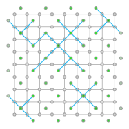
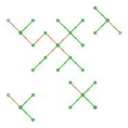
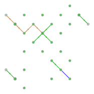
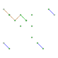
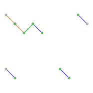
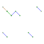
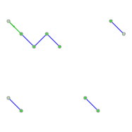
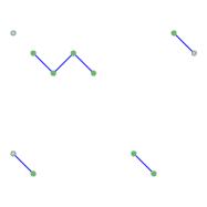
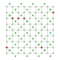
Figure 10: Graphical representation of the forest peeling from a spanning forest chosen from the set of erasure errors from FIG.9.

5.2.3 Performance and threshold

In FIG. 11, the performance of the rotated planar code over depolarizing noise when decoded with the UF decoder is presented. Inspecting the figure, and TABLE 2, it can be seen that the code thresholds achieved by this decoding method are smaller than the ones obtained using the MWPM decoder for all biases considered (recall TABLE 1). Interestingly, the UF decoder always returns an error suited for the syndrome facilitated, nevertheless, this error does not always result in the error of minimum weight. Thus, the decrease in performance when compared to the MWPM can be explained by the instances in which the peeling decoder misses to relate closest non-trivial syndrome elements. Several attempts have been done by the community in order to diminish the non-optimal choices made by the UF decoder while keeping its low complexity. At the time of writing, a popular approach towards this goal consists in reweighting the edges of the graph [139, 87]. The reweighting is usually done by previously running some method in order to estimate which data qubits are more prone to have suffered from errors for such syndrome measurement. With such information, the edges representing data qubits that are more prone to errors will have lower weights, which implies that the vertices they connect are closer. Thus, when growing clusters in the syndrome validation phase, the radial growth is fixed and clusters are more prone to grow towards likely to fail data qubits. For example, the so-called belief-find decoder uses a belief propagation method to estimate such information and then continues to decode the error by the UF method [87].

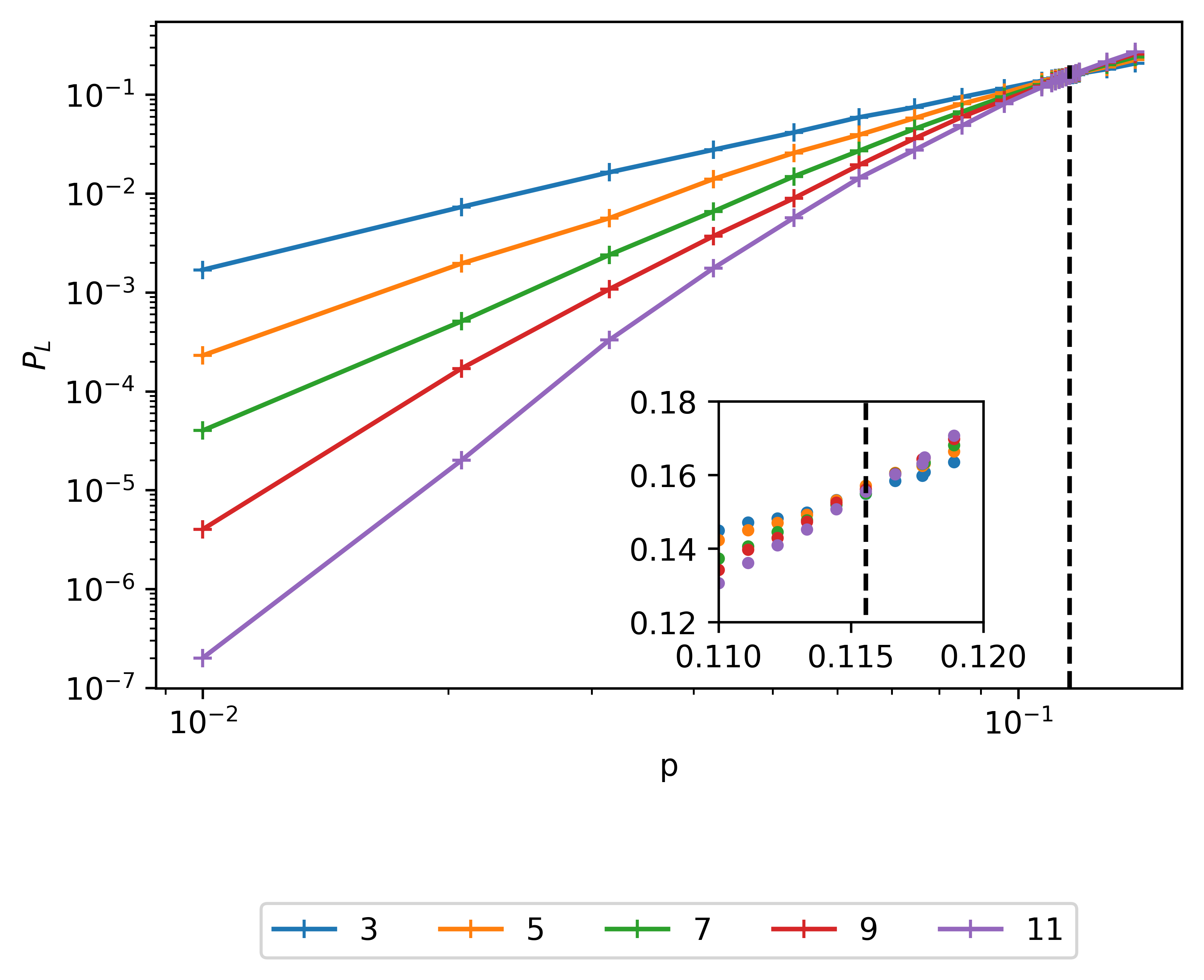
Figure 11: Logical error probability with dependence on the physical error probability from the UF decoding method under depolarizing noise.

$\eta$	$p_{th}$
1/2	0.116
1	0.114
10	0.080
100	0.078
1000	0.077

Table 2: Probability threshold values for different biases in the rotated planar code under the UF decoding scheme.

5.2.4 Measurement errors

As explained before, the so-called measurement errors due to imperfect measurement operations and propagation of errors in stabilizer measurement stage have been considered for the MWPM decoder. In the case of the UF decoder, this type of effects have also been taken into account by considering multiple syndrome measurements for a single decoding round, refer to Appendix B for an extended description. In this sense, syndrome validation and peeling are realized over the space-time graph that is obtained. Reweighting methods for a better performance of the UF decoder over those space-time graphs have been discussed too [87, 139]. In addition, and due to the fact that the complexity of the algorithm increases when the space-time graph is considered, truncated UF methods have also been proposed to maintain the fast decoding while not losing too much in terms of decoding success [139].

Ultimately, UF proves to be a very efficient method for decoding the surface code and stands as a fair counterpart to the conventional MWPM decoding process. So much so, that the cluster growth process in the syndrome validation has inspired new methods for optimizing the computational complexity of the minimum-weight perfect matching decoder [57, 118]. Moreover, the UF-decoding method also yields the great advantage of successfully taking into account erasure errors. Were a surface code to undergo a mixture of Pauli and erasure errors, the only difference with the process explained before would be that on the syndrome validation step, there would also be erasure errors, frozen from the beginning, in the form of edges that would join to whichever cluster gets in contact with them. Lastly, there have also been studies trying to strictly relate the conditions under which UF will return the same error as the MWPM method [130] and even more, it has been studied as a possible decoding method for QLDPCs [140], although the complexity problem in this specific case has yet to be addressed. Due to its low complexity and high threshold, as of the moment of writing, the UF method seems to be a promising candidate for early experimental real-time surface code decoding.

5.3 Belief Propagation

Belief Propagation (BP) is a message-passing algorithm that can be used to solve inference problems on probabilistic graphical models [141]. It is also sometimes referred to as the Sum-Product Algorithm (SPA) [142, 143], a more general-purpose algorithm that computes marginal functions associated with a global function. Although the terms BP and SPA are essentially interchangeable, throughout this paper we will use BP to refer to the algorithm employed to decode error correction codes.

Error correction codes, irrespective of being applied in a quantum or classical paradigm, can be represented by bipartite graphs known as factor graphs. A factor graph $G=(N,E)$ is defined by a set of nodes $N=V\cup C$, where $V,C$ represent two distinct types of nodes known as variable and check nodes, respectively, and a set of edges $E$. Against this backdrop, BP can be used to approximate the problem of Maximum Likelihood Decoding (MLD) by exchanging messages over the factor graph representation of an error correction code. If BP runs over a graph that is a tree, it will converge to the exact MLD solution in a time bounded by the tree’s depth. In scenarios where this does not hold, i.e., when the algorithm is run over a loopy factor graph and convergence cannot be achieved, BP has proven to be a good heuristic decoding method, especially when the typical size of the loops in the graph is large.

5.3.1 BP: Specifics

Earlier we introduced QMLD and DQMLD as the two possible domains of QECC decoding problems. We also mentioned how QMLD and DQMLD are both intractable problems (QMLD belongs to the NP-complete complexity class while DQMLD belongs to the #P-complete complexity class). This means that decoding algorithms generally work by finding solutions to good aproximations of the decoding problem. This is precisely the operating principle behind BP works. In the classical context, BP decoders work by solving an approximation of the classical MLD problem known as bit-wise MLD [54]. In the quantum context, an analogous principle is employed: instead of tackling QMLD, we use classical BP decoders and the symplectic representation to solve the problem of qubit-wise MLD. Note that, not only are we not solving QMLD exactly, but we are also ignoring the phenomenon of degeneracy (an optimal quantum decoder would address DQMLD, not QLMD).

Qubit-wise MLD is different from QMLD in that, instead of looking for the most likely error given the syndrome, i.e., looking for the global optimum, we will look for the qubit-wise most likely error, i.e., looking for the marginal optimum. This entails maximizing the probability of each individual qubit given a particular syndrome bit. Qubit-wise MLD can be written as:

$$\hat{E}_{i}^{\text{bw}}=\operatorname*{\arg\max}_{E_{i}\in\mathcal{G}_{1}}\sum_{E_{1},\ldots,E_{i-1},E_{i+1},\ldots,E_{n}}P(E_{1}\dots E_{n}|s),$$ (14)

where the qubit-wise most likely error is obatined by running through all vaues of $i$: $\hat{E}^{\text{bw}}=[\hat{E}^{\text{bw}}_{1}\ldots\hat{E}^{\text{bw}}_{n}]$. In general, $\hat{E}^{\text{bw}}$ need not coincide with the global optimum obtained by solving (7) [144].

Although computing solutions to (14) is also difficult, this task is amenable to BP. Given a factor graph representation of the parity check matrix of a code, BP can run over the aforementioned graph and obtain the qubit-wise most likely error in polynomial time. Assuming that we are working with CSS codes, note that the rotated planar code belongs to this class, (refer to [144, 54] for a more general description), the BP decoding problem can be understood as the execution of two classical BP decoders, one for $X$-errors and the other for $Z$-errors. Thus, we can describe the iterative schedule of BP decoding as if applied to a classical code. To begin, the BP algorithm requires an error syndrome $s$ and the channel error probability distribution. The error syndrome is computed as $s=H\cdot E$, where $H$ denotes the parity check matrix of the classical code and $E$ represents the error, and is a length $n-k$ binary vector. Each of the entries in the syndrome vector is assigned to a check node. Conversely, the channel error probability distribution is made available to the variable nodes. In this sense, the BP decoder operates by executing the following instruction schedule:

1. At a given decoding iteration $t$, each variable node, $v_{i}$, sending out a message, $\mu^{t}_{v_{i}\rightarrow c_{j}}$, to the check nodes, $c_{j}$, it is connected to. In the first decoding iteration, $t=1$, this message is equal to the a priori bit error probability, given by the noisy quantum channel in consideration. This message is generally expressed in the log-likelihood domain as

   $$\mu^{1}_{v_{i}\rightarrow c_{j}}=l_{\text{ch}}(E_{i})=\text{log}(\frac{p(E_{i}=0)}{p(E_{i}=1)}),$$

   where $i\in[1,\ldots,n]$, $j\in[1,\ldots,n-k]$, and the term $l_{\text{ch}}$ represents a priori channel log-likelihood ratio (llr). Note that here we used the slight abuse of notation $E_{i}$, which refers only to a $X$-error or $Z$-error due to the CSS structure of the code, i.e. $E_{i}=E_{i}^{x/z}$. At future iterations, the message sent from a variable node to neighboring check nodes is given by

   $$\mu^{t}_{v_{i}\rightarrow c_{j}}=l_{\text{ch}}(E_{i})+\sum_{k=1}^{\sigma-1}\mu^{t-1}_{c_{k}\rightarrow v_{i}},$$

   where $\mu^{t-1}_{c_{k}\rightarrow v_{i}}$ are messages received from check nodes in the previous iteration and $\sigma$ is the degree (number of connections) of the variable nodes. Note that the sum goes to $\sigma-1$ because the message received from check node $c_{j}$ in iteration $t-1$ is not considered.

2. Once all these initial messages have been received by the check nodes, every check node will reply to all neighbouring variable nodes with the following message:

   $$\mu^{t}_{c_{j}\rightarrow v_{i}}=(-1)^{{s}_{j}}2\text{atanh}[\prod_{k=1}^{\psi-1}\text{tanh}(\mu^{t}_{v_{k}\rightarrow c_{j}})],$$

   where $\psi$ represents the degree of the check nodes, $t$ represents the BP iteration, and $s_{j}$ denotes the syndrome bit associated to that particular check node. Notice how the product required to compute $\mu_{c_{j}\rightarrow v_{i}}$ only goes to $\psi-1$. Once again, this is because the prior variable node message received from the node the current message will be sent to should not be considered.

3. Once all check node messages have been received, variable nodes can compute their llrs (also referred to as beliefs or marginals), which we use to estimate (14). This is done as

   $$l^{t}_{\text{ap}}(E_{i})=l_{\text{ch}}(E_{i})+\sum_{k=1}^{\sigma}\mu^{t}_{c_{k}\rightarrow v_{i}}.$$

   Note how the a-posteriori llrs are a combination of the initial a-priori channel llrs and decoding information processing.

4. At this point we check whether more decoding iterations are needed. First we obtain the estimate $\hat{E}^{\text{bw}}=[\hat{E}^{\text{bw}}_{1}\ldots\hat{E}^{\text{bw}}_{n}]$ by making hard decisions on the beliefs $l^{t}_{\text{ap}}(E_{i})$. These hard decisions commonly follow that negative llr, $l^{t}_{\text{ap}}(E_{i})$, relates to the fact that the estimated probability of error is higher than no error for such qubit. Then, we compute the syndrome associated to the decoding estimate as

   $$\hat{s}=H\cdot\hat{E}^{\text{bw}}.$$

   If $\hat{s}=s$ then decoding has been successful and the BP algorithm is halted. If not, then additional iterations will be run until either $\hat{s}=s$ or a maximum number of iterations is reached.

5.3.2 Aftermath of neglecting DQMLD

The excellent performance of BP as a decoding algorithm for classical random-like codes, such as LDPC codes and turbo codes [38, 145], is well-documented. In fact, classical LDPC codes are essentially capacity-achieving when decoded via BP [145]. For this reason, along with their finite-rate guarantees, the design of so-called ‘good’ quantum LDPC codes has been a long-pursued topic in the field of QEC. Although the existence of sparse codes exhibiting such favorable parameter scaling remained unproven for the past two decades, groundbreaking results by Panteleev and Kalachev [48] as well as [146, 147, 148] have finally shown that quantum analogues of robust LDPC codes do actually exist. However, this only addresses half of the problem (the code design aspect), as there are further quantum-specific challenges in terms of decoding. Quantum codes manifest a phenomenon known as degeneracy [54, 128, 67, 149, 144, 80, 46], which has no classical equivalent. This poses a quandary that the classical version of BP cannot resolve, as it is designed for a classical environment in which degeneracy is not present.

Recall that degeneracy in the context of QEC refers to the fact that errors $E\in\mkern 1.5mu\overline{\mkern-1.5mu\mathcal{G}\mkern-1.5mu}\mkern 1.5mu_{n}$ that differ by a stabilizer element (errors that belong to the same logical coset) have the same effect on the code and, thus, are correctable by the same recovery operation. An optimal decoding strategy for degenerate codes should weigh the probability of each logical coset and pick an operator from the most probable one (the operator itself is irrelevant, what matters is picking the right equivalence class). This nuance is critical, as it highlights the differences between optimal decoding for degenerate quantum codes: DQMLD and non-degenerate quantum codes: QMLD. Applying the QMLD rule to a degenerate quantum code is suboptimal, as the operator with highest probability need not belong to the coset with highest probability. This performance difference is further aggravated if a BP decoder is employed to solve QMLD. This is due to the fact that degenerate quantum codes can simultaneously exhibit an error probability that is sharply peaked over a logical coset (which would lead to great performance under DQMLD) and that has a broad marginal distribution over individual qubits, which given the large number of low and similarly weighted operators of such codes, would severely hinder a BP decoder. The existence of the aforementioned operators and their equivalence under BP decoding lead to the peculiar symmetric degeneracy error phenomenon [144], which is also referred to as split-belief [122] or Quantum Trapping Set (QTS) [150, 151]. Quite frankly, if a code is degenerate enough (if the weight of its generators is substantially smaller than its distance), split beliefs can put the proverbial nail-in-the-coffin for a BP decoder in this context. This cannot be better exemplified than by the fact that that the surface/toric code exhibits no threshold under BP decoding [122]. Surface codes are degenerate by nature, becoming even more so as their size is increased (the weight of their stabilizer generators remains the same but the distance grows). This makes the split-belief phenomenon more prevalent for larger surface codes, explaining the absence of a threshold for this family of codes under BP decoding, as can be seen in FIG. 12.

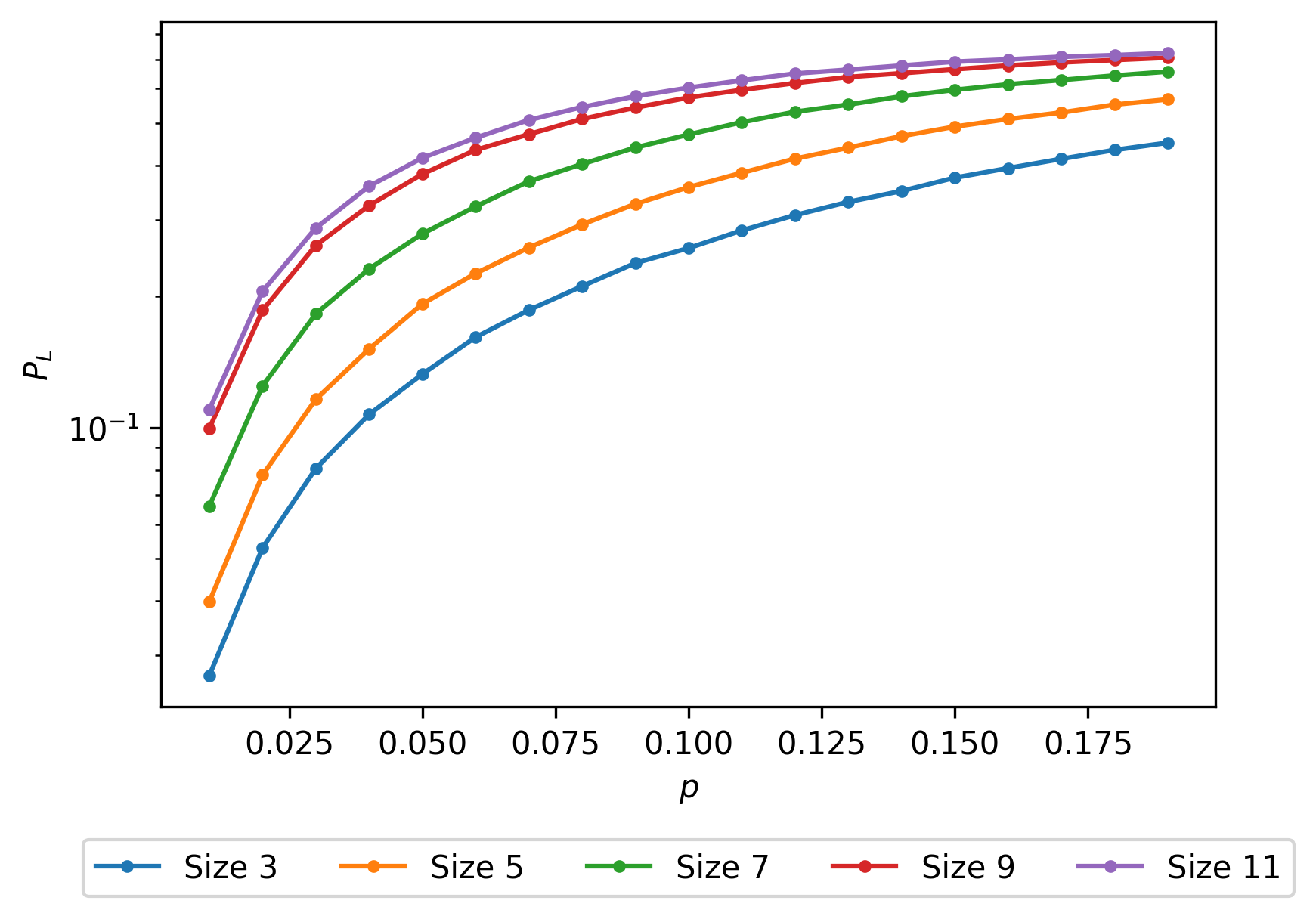
Figure 12: Logical error probability with dependence on the physical error probability under depolarizing noise with BP decoding.

Split-beliefs have been analyzed in the literature [144, 150, 151] and their impact has been successfully alleviated through myriads of post-processing routines added to general BP decoding. The most successful of these modified BP-based decoding techniques is known as BP-OSD [46]. The performance increments this strategy provides have made it the front-runner in the conversation of a general purpose decoder for QLDPC codes. In fact, the toric code actually exhibits a threshold when decoded via this more sophisticated algorithm. In consequence, this begs the question of whether BP-OSD can compete with the other decoding strategies for the planar code that we have seen thus far.

5.3.3 Enhanced Belief Propagation: Quantum Ordered Statistics Decoding

The post-processing algorithm known as Ordered Statistics Decoding (OSD) [152, 153] was originally designed to improve the performance of small classical codes, as well as to lower the error floors of certain LDPC codes. It was later adapted to the quantum paradigm by Panteleev and Kalachev in [46], where the authors successfully devised the so called qOSD routine via specific modifications to the classical OSD algorithm. In a similar fashion to other post-processing routines for sparse quantum codes, qOSD only works in conjunction with a BP decoder; i.e., it requires the soft outputs of a BP decoder in order to function. For this reason, the decoding routine that combines both BP and qOSD is generally referred to as BP-OSD. In later work, BP-OSD was shown to work well for Toric codes and a novel class of semi-topological codes [122], and recently, it has also been shown to be a valid decoding strategy for bias-tailored QLDPC codes [154]. The authors of [122] also made their implementation of BP-OSD public, which marked the first open-source demonstration of this decoding algorithm.

As is done in [122], for the sake of notational simplicity, we describe OSD post-processing as applied to the classical decoding problem

$$s=H\cdot e.$$ (15)

It is obvious that this framework is equally applicable (albeit with minor programming modifications) to decoding the $X$ and $Z$ components of a CSS code or directly decoding over the entire parity check matrix of a non-CSS code.

The OSD post-processing algorithm is called upon whenever BP fails to produce an estimate $\hat{e}$ that matches the measured syndrome. Hence, our starting point is the following: after attempting to decode the measured syndrome $s$ via BP we end up with the incorrect estimate of the error $\hat{e}$. The estimate is known to be erroneous since its syndrome does not match the true syndrome. However, the fact that $s\neq H\cdot\hat{e}$ does not imply that all components of $\hat{e}$ are wrong, a rationale that OSD will exploit to find a valid solution to (15).

We begin by introducing a necessary set of concepts. We will call the set of indices $[I]$ for which $H\cdot e_{I}=H\cdot\hat{e}_{I}$ the most reliable information set. The complement of this set $[\bar{I}]$, all those indices for which $H\cdot e_{\bar{I}}\neq H\cdot\hat{e}_{\bar{I}}$, will thus be referred to as the least reliable information set. As we explain in what follows, OSD post-processing exploits the concept of reliable information sets to solve the linear system described by (15). The parity check matrix $H$ of a quantum error correction code is a rectangular matrix that does not have full column-rank, making it impossible to solve $s=H\cdot\hat{e}$ via matrix inversion. However, the system described by an appropriate set of $n-k$ linearly independent columns $[S]$ of $H$ is actually solvable:

$$s=H_{[S]}e_{[S]},$$ (16)

can be solved as

$$H^{-1}_{[S]}s=e_{[S]},$$ (17)

(note that $H_{[S]}$ is a full-rank matrix). For every choice of $[S]$, the basis of linearly independent columns, we will obtain a unique solution $e_{[S]}$, that satisfies (16). Against this backdrop, we can understand what OSD post-processing is about: if a full-column rank subset of the parity check matrix can be found and used to solve (16) via matrix inversion, we will always find a solution $e_{[S]}$ that produces a matching syndrome $s$. Additionally, because this solution is unique, any symmetries that might hinder BP decoding (like those that cause split beliefs) are now broken.

Naturally, the next question becomes how do we pick the basis $[S]$ in a way that guarantees that this solution is actually ‘good’, i.e., that it is the lowest weight operator associated to the measured syndrome. It is at this point that the previously introduced concept of reliable sets is applied. More precisely, we can use the soft-values (a posteriori llrs) produced in the final BP decoding iteration to rank the bits from most likely to least likely of being flipped (lowest to highest llr values). We can then apply this order to re-arrange the parity check matrix of the code into a new matrix $\Lambda$. It is clear that the basis $[J]$ defined by the columns of the first full column rank submatrix $\Lambda_{[S]}$ of the rearranged matrix is the least reliable basis, as it is obtained from the indices of the linearly independent columns associated to the least reliable set of bits. By picking the OSD submatrix in this way, we are guaranteed to find a low weight solution to the syndrome equation. At this point, instances of the OSD algorithm with varying degrees of complexity, denoted as order-$w$ OSD or OSD-$w$, where $w\in[0,\ldots,K]$ and $K\in\mathbb{N}$, can be applied to search for the lowest weight solution to (15). In what follows we detail the functioning of OSD post-processing and the differences between the lowest order version of OSD, OSD-$0$, and higher order intances, OSD-$w$.

OSD-0: Assume the following, after measuring a given syndrome $s$ for a specific code with parity check matrix $H$, we have decoded via BP and obtained an estimate of the error $\hat{e}$, which unfortunately does not produce a matching syndrome: $s\neq H\cdot\hat{e}$. In this context, we would execute OSD, which would operate as follows:

1. Take the soft-outputs of the BP decoder given by $l_{i,\text{ap}}=\frac{P(e_{i}=0|\mathbf{s})}{P(e_{i}=1|\mathbf{s})},\ \forall i\in{0,\ldots,n}$, and order them from most-likely to least-likely to have been flipped (increasing order of magnitude). Store the list of bit-indices $[\text{OG}]$, as this defines the least reliable information set of bits.

2. Re-arrange the columns of the parity check matrix of the code according to the ranking defined by $[\text{OG}]$. We will denote this new matrix by $\Lambda$.

3. Select the first $n-k=\text{rank}(H)$ linearly independent columns of $\Lambda$ to obtain the submatrix $\Lambda_{[J]}$. The list of indices associated to these columns defines the least reliable information set of bits $[J]$. Note that these columns must be linearly independent, else $\Lambda_{[J]}$ will not have full-column rank.

4. Invert $\Lambda_{[J]}$ into $\Lambda^{-1}_{[J]}$. Calculate the solution $e_{[J]}$ to the OSD syndrome equation as $\Lambda^{-1}_{[J]}s=e_{[J]}$.

5. The complete solution to the decoding problem is $\mathbf{e}_{\Lambda_{0}}=[e_{[J]},e_{[\bar{J}]}]$, where $J$ and $\bar{J}$ denote the least and most reliable information set of bits, respectively. Knowing that $e_{[J]}$ satisfies $\Lambda_{[J]}e_{[J]}=s$ then it is easy to see that $\Lambda\mathbf{e}_{\Lambda_{0}}=\Lambda[e_{[J]},\mathbf{0}]=s$.

6. The last step is to take the solution $\mathbf{e}_{\Lambda_{0}}=[e_{[J]},\mathbf{0}]$, and map it to the original bit-index order: $\mathbf{e}_{\Lambda_{0}}\rightarrow\mathbf{e}_{\text{OSD-0}}$. We call the rearranged vector, $e_{\text{OSD-0}}$, the OSD-0 solution.

In FIG. 13, an example is provided where a specific error produces a syndrome which is later decoded finally obtaining a recovered error. In the top row, the error and the syndrome within the surface code are introduced, data qubits, $X$ and $Z$-checks are labelled in black, green and orange colors respectively. In the second row, one can see a graphical representation of the BP method, where messages are sent from data qubits to checks and vice versa. Notice, how there are two grey circles for each data qubit label, that is because the two BP graphs are independent, and so each data qubit will have two resulting marginal probabilities, one for the $X$-operators and another one for the $Z$ ones. In the following row, the resulting marginal probabilities are represented within the data qubits of the surface code with $X$-check qubits and $Z$-check ones. On the left surface code a data qubit being redder indicate its marginal probability of recovering an $X$-operator being larger, and thus its llr being lower, and whiter otherwise. The same rules go by the $Z$-check surface code on the right. On the following row, the matrix $\Lambda$ is represented. The chosen data qubits are the ones which represent the independent columns with the higher marginal probabilities, the four columns on the left are extracted from the $X$-check subgraph and the remaining four from the $Z$-check subgraph, as indicated by the labels on top of the matrix. This matrix is inverted following the earlier described process, reaching a recovered error which is depicted in the last row. Notice how the error is not the same set of Pauli operators as the inputted one, nevertheless, it is within the same stabilising group, and thus, successfully corrects the error.

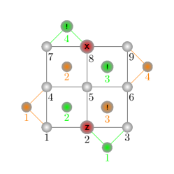
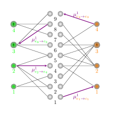
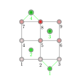
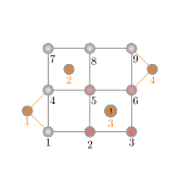
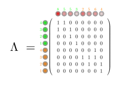
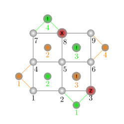
Figure 13: Graphical description of a BPOSD-0 process for a specific syndrome in a 3x3 surface code.

OSD-$\mathbf{w}$: Higher order OSD is similar to OSD-$0$, the difference being that we now consider solutions $\mathbf{e}_{\Lambda_{w}}=[e_{[J]},e_{[\bar{J}]}]$ where $e_{[\bar{J}]}\neq\mathbf{0}$. OSD-$w$ begins by running the first five steps of OSD-$0$ and computing $e_{[J]}$, which for the sake of notation we will now denote by $e^{w=0}_{[J]}$. Once this is done, different candidates $\mathbf{e}_{k}$ can be found by making choices for $e_{[\bar{J}]}$ and solving

$$\mathbf{e}_{\Lambda_{w}}=[e_{[J]},e_{[\bar{J}]}]=[e^{w=0}_{[J]}+\Lambda^{-1}_{[J]}\Lambda_{[\bar{J}]}e_{[\bar{J}]},\ e_{[\bar{J}]}],$$ (18)

where $\Lambda_{[\bar{J}]}$ is the submatrix obtained by taking the columns of $\Lambda$ indexed by $\bar{J}$. The solution $\mathbf{e}_{w}$ given in (18) satisfies the OSD syndrome equation

$$\Lambda\mathbf{e}_{\Lambda_{w}}=s$$ (19)

for any choice of $e_{[\bar{J}]}$. The premise behind OSD-$w$ (considering $e_{[\bar{J}]}\neq\mathbf{0}$) is to find solutions $\mathbf{e}_{\Lambda_{w}}$ of lower Hamming weight than $\mathbf{e}_{\Lambda_{0}}$. The $e_{[\bar{J}]}\neq\mathbf{0}$ component has dimension $n-\text{rank}(H)$, implying that testing all possible configurations for $e_{[\bar{J}]}$ is intractable beyond a small value of $n$. For this reason, it is important to design a strategy that makes good choices for the $e_{[\bar{J}]}$ candidates. This is best approached using the so called combination sweep strategy. This greedy search method works as follows:

1. At the start of the search, the OSD-$w$ solution is equal to the unordered OSD-$0$ solution: $\mathbf{e}_{\Lambda_{w}}=\mathbf{e}_{\Lambda_{0}}$.

2. Sort the bits in the $e_{[\bar{J}]}$ subvector of the solution according to the soft-outputs of the original BP decoding attempt. Note that this step is already built into OSD-0 when re-arranging the parity check matrix according to the BP outputs.

3. Test all possible weight-$1$ configurations of $e_{[\bar{J}]}$. There are a total of $n-\text{rank}(H)$ weight-$1$ candidates. If the weight of any of the candidates is lower than the weight of $\mathbf{e}_{\Lambda_{0}}$, update the choice of $\mathbf{e}_{\Lambda_{w}}$.

4. Try all possible weight-$2$ configurations in the first $w$ bits of $e_{[\bar{J}]}$. Obviously, the order $w$ will be upper bounded by $n-\text{rank}(H)$ the dimension of $e_{[\bar{J}]}$. The number of candidates is given by the binomial coefficient $\binom{w}{2}$. If the weight of any of the candidates is lower than the weight of the current choice for the solution, update the choice of $\mathbf{e}_{\Lambda_{w}}$.

5. The final step is analogous to that of the order $0$ version: map the solution to the original bit-index order accordingly: $\mathbf{e}_{\Lambda_{w}}\rightarrow\mathbf{e}_{\text{OSD-w}}$.

OSD-$w$ entails testing a total of $n-\text{rank}(H)+\binom{w}{2}$ candidates for $\mathbf{e}_{\Lambda_{w}}$, out of which the minimum Hamming weight solution, or at least a better choice than $\mathbf{e}_{\Lambda_{0}}$, will have been found. As the order $w$ of the combination sweep strategy is increased, the likelihood of finding the solution of minimum Hamming weight to (19) increases. At the same time, this also implies additional computational demand, negatively impacting the complexity of the algorithm and its runtime performance.

5.3.4 OSD Complexity

In [46], the authors show that most of the performance improvements provided by qOSD postprocessing are achieved with OSD-0. While increasing the order $w$ of the algorithm yields benefit over setting $w=0$, for various QLDPC code families the improvement provided by running the algorithm with $w>0$ is marginal. It is important to mention that in [46], the authors use a different algorithm to the combination sweep strategy [122]. Instead, they apply an exhaustive approach where they test all possible permutations in the first $w$ bits of $e_{[\bar{J}]}$. Given that OSD-$0$ requires the solving of a linear system, its complexity will be at most $O(n^{3})$ (although there are matrix inversion algorithms with better complexity [155], they are quite impractical). The exhaustive approach to OSD-$w$ has a complexity in the general case of $O(n^{3}+n2^{w})$. Although the combination sweep also has an edge in terms of complexity ($\approx O(w^{\alpha}n^{3})$), it is likely that OSD-$0$ is the only version of the algorithm that can be successfully implemented in a real time system [122, 156]. Recently, an OSD-inspired reduced complexity approach known as stabilizer inactivation has been proposed. In [157] the authors showed that this strategy, which has $O(n^{2}\text{log}n)$ in the worst case, achieved a higher threshold for the family of generalized bicycle codes.

5.3.5 Performance and threshold

As has been previously seen in FIG. 12, the BP decoding method has no probability threshold by itself and so is not a usable decoding method for the decoding of the surface code. Nevertheless, considering BPOSD-0 yields an enhancement which produces a probability threshold of $0.139$ under depolarizing data qubit noise. This result can be seen in FIG. 14. This threshold can be further expanded when considering higher BPOSD orders at the expense of a higher complexity. Moreover, the BPOSD method is also compromised when considering $Z$-noise bias, which can be explained by the $Z$-check subgraph becoming more dense than the $X$-check one and thus being more prone to failure. Table 3 reviews several thresholds for three different ordered statistics decoding processes under different biases.

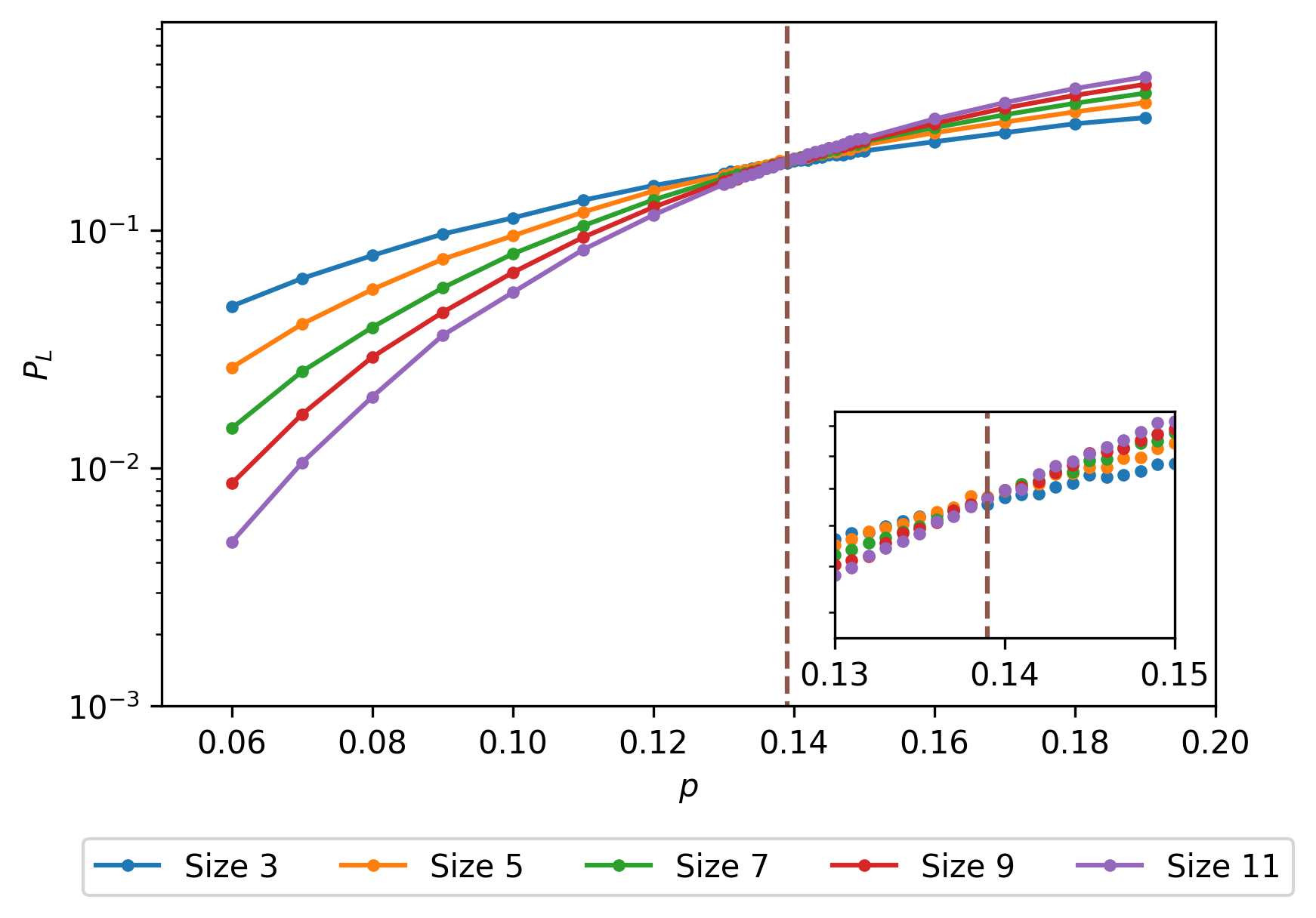
Figure 14: Logical error probability with dependence on the physical error probability under depolarizing noise with BPOSD-0 decoding.

$\eta$	$p_{th}$
1/2	0.139
1	0.138
10	0.098
100	0.094
1000	0.092

Table 3: Probability threshold values for different biases and orders in the rotated planar code under the BPOSD-0 decoding scheme.

5.3.6 Measurement errors

There have been many proposals for handling circuit-level noise by using belief propagation. An important proposal for handling this type of errors in the surface code is the decoder deemed as belief-matching [87]. This decoder is base on a combination between the BP and MWPM algorithms, idea that was previously explored in [158] with perfect syndrome measurements. The original belief-matching algorithm achieved a $17.76\%$ threshold for the rotated planar code when depolarizing noise was considered over the data qubits. The decoding complexity of the algorithm was maintained when compared to MWPM when parallel processing was allowed [158]. Due to the impressive performance of this BP+MWPM approach, such method was generalized to handle noisy gates and SPAM errors in [87], resulting in one of the most vainglorious algorithms for obtaining logical qubits in such planar architecture codes. The basic idea behind the belief-matching algorithm is similar to the BPOSD decoder in the sense that the soft ouptuts of the sum-product algorithm are used for the posterior decoding algorithm to make use of them. In this sense, the weights of the the graph in the MWPM decoder are produced by using such a posteriori information. Regarding the generalization of the belief-matching for circuit-level noise, the authors discussed how to construct the circuit-level Tanner graph that takes the measurement circuits of the surface code into account so that belief propagation can be run over such graph and then use the soft output for obtaining the MWPM solution [87]. Note that $\mathcal{O}(d)$ measurement rounds are required for this. The authors found a threshold of $0.94\%$ for the belief-matching algorithms with circuit level noise, which is comparable to the belief-find decoder also proposed in such article, which follows the same procedure but using UF instead of MWPM and achieves a threshold of $0.937\%$ [87]. The authors discuss that their performances are similar due to the fact that most of the information needed for decoding is provided by the BP part of the algorithm.

Another approach to deal with noisy syndromes is to consider soft syndrome information for the BP graph used for decoding as it was done for QLDPC codes in [159]. In such work, the authors discuss the fact that when a measure met is noisy, the input information of the Tanner graph regarding the information of the syndrome can be soft, i.e. a probability distribution conditional to the obtained noisy measurement. Therefore, the fact that the measurement outcome might not be precise is also fed to the BP algorithm. However, this study only considered the fact that the noisy measurements are a result of SPAM errors, neglecting circuit level noise. The authors discuss that this is considered to be future work in this direction. Interestingly, such paper was based on the previous work by Pattison et al. that discussed the use of soft measurement information in the context of MWPM and UF for surface codes [160]. The authors concluded that their modified decoders using soft information improved the threshold obtained by hard decision decoders for the circuit-level noise considered. In this sense, considering this approaches for BP decoders discussed for the surface code might be an interesting path to follow for dealing with circuit level noise.

Finally, single-shot decoding using BPOSD was investigated for the 4D toric code in [161]. Single-shot decoding refers to estimating the error when noisy measurements are present in a single measurement round, i.e. without needing to measure the usual $\mathcal{O}(d)$ rounds. In such article, the authors propose to decode data qubit errors and noisy syndrome measurements altogether in a single stage via the BPOSD decoder. The authors discuss that they obtain better thresholds than using multiple-measurements and other single-shot decoder such as the cellular automaton decoder. However, they use a phenomenological noise model for faulty syndrome measurements as discussed before, i.e. they do not consider full circuit-level noise, which they consider to be future work [161]. Single-shot decoding is being actively investigated at the time of writing, specially from the point of view of QLDPC codes [162, 163, 164, 165]. This approach was originally proposed for some families of topological codes, and due to its advantage in terms of measurement rounds and, presumably, performance, seems to be interesting to study more codes that may admit this kind of decoding to deal with circuit-level noise.

5.4 The Tensor Network decoder

Tensor Network (TN) decoders are decoding methods, proposed by Bravyi et al. for the surface code, that aim to resolve the DQMLD problem, i.e. to estimate which is the most probable logical coset based on the syndrome information [121]. Note that, up to this point, all decoders considered have followed a QMLD logic, that is, their aim has been to seek for the most probable Pauli error (QMLD) since, as has been seen earlier, the error recovery problem contemplating error logical classes (DQMLD) belongs to the $\#P$ complexity class [55]. For this reason, the TN decoder is also usually referred as the maximum likelihood decoder (MLD)[121]. Fortunately, surface codes admit a natural representation in terms of Tensor Networks (TN) [166], feature that can be used for approximating the DQMLD problem targeting the most probable error coset. Decoding quantum error correcting codes with TNs was first considered in [167], where the authors described for the first time the equivalence between decoding a quantum code and contracting a TN for quantum turbo, polar and branching multiscale entanglement renormalization ansatz (MERA) codes [168, 169]. Later, the TN decoding was particularized for the planar code in [121], and, afterwards, in [170], the method was expanded to the rotated planar code yielding significant results. Lastly, in [171], the method was generalized to any quantum 2D code.

Planar codes are not the only class of topological codes that admit the TN decoding methods as, in general, those admit a natural representation in terms of 2D Projected Entangled Pair States (PEPS) [172]. For instance, the ground states of the Toric Code Hamiltonian, codifying two logical qubits, can be written exactly as PEPS with low bond dimension, and the same is true for all other surface codes such as quantum double models, color codes, and even string-net models [173]. This analytical correspondence implies that decoding such codes can be done using standard TN techniques, in particular those related to the contraction of 2D TNs. Such algorithms have been used widely in the calculation of partition functions of 2D classical lattice models [174, 175], as well as in the calculation of expectation values of 2D quantum states on a lattice [172, 176]. Take for instance the straightforward example of the Toric Code. The expectation value of loop operators around the torus geometry decode the value of the logical qubits, in a completely analogue way to the expectation value of Wilson loop operators in lattice gauge theories. As such, these loop operators are built from tensor products of Pauli matrices along the sites on a loop, and the TN contraction involved to estimate them can be done via usual contraction methods for 2D TNs.

In broad terms, the idea behind TN decoding consists in recovering an error $E_{rec}$ that shares the observed error syndrome in a quick manner so that when combining it with the actual channel error the resulting element lays in the normalizer of the code. Once this is done, the probability of the logical error cosets of the normalizer are computed to select the most probable one. For the specific case of codes encoding a single logical qubit (such as the rotated planar code), there will be four logical cosets: $I_{L},X_{L},Y_{L}$ and $Z_{L}$. It is worth mentioning that $E_{rec}$ does not need to be the most probable error since its unique purpose is to transport the error to the zero syndrome coset [128]. After $p(E_{rec}I_{L}),p(E_{rec}X_{L}),p(E_{rec}Y_{L})$ and $p(E_{rec}Z_{L})$ are computed, the most probable error class, $\mathcal{L}$, determines the recovery operation $\hat{E}=E_{rec}\mathcal{L}$.

5.4.1 Introduction to TNs

In order to better understand the functioning of the TN decoder, we will first briefly introduce some generic terms about tensor networks. TNs are a class of variational wave functions used in the study of many-body quantum systems in which the quantum relation from tensor to tensor is known [166]. TNs are used in many research fields for studying complex and correlated systems with large configuration spaces. How they work is based on the fact that there are configurations much more significant than others, and so, given a certain threshold, one can omit the least reliable configurations in order to work with a reduced and manageable subspace.

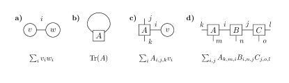
Figure 15: Some examples of tensor operations. a) indicates a scalar product of two vectors, b) indicates the trace of a matrix, c) indicates the product of a vector with a matrix and d) indicates a matrix product state.

TNs accept an intuitive notation. FIG. 15 depicts some examples of tensors represented through various plots, where vectors are represented as circles, and matrices and higher order tensors, as squares. In a TN, some, or all the indices can be contracted according to a specific pattern, as shown in FIG. 15. If all the indices are contracted, the TN results in a scalar, as in the case of the two first examples of FIG. 15. The lines connecting tensors from one to the other represent the indices such that there is a sum over all their possible values, whereas lines that are not connecting to anywhere represent free indices. Those indices that correspond to the original physical Hilbert spaces are called physical indices, and the rest (connecting the different tensors with each other) are called bond indices, and are responsible for the entanglement in the quantum many-body wavefunction. The range of values of a bond index is called bond dimension, following common TN terminology [166, 121].

Consider now the following case: we have a 2D tensor network such as the one showed in FIG. 16, which is the one encountered when computing expectation values of a projected entanglement pair state (PEPS). The constituent tensors on the bulk have bond dimension 4, while the ones on the boundary have lower bond dimensions. One can consider the left-most (or right-most) column as a matrix product state (MPS) and columns within the bulk of the PEPS as matrix product operators (MPO). When contracting the left MPS with its nearest MPO, the overall 2D TN will be reduced by one column as shown in FIG. 16, and for the new column which is obtained the vertical bond dimension will have increased in an exponential manner. Contracting the entire 2D TN will most likely be an unfeasible challenge as a result of the exponentially increasing bond dimension. Fortunately, we can still obtain meaningful results for continuous column contraction while avoiding an exponential growth [177, 178]. For the cases we consider, this is made by using the QR matrix decomposition altogether with the singular value decomposition (SVD), which is used to truncate the vertical bond-dimensions [121, 179]. Truncating the bond dimension of the column contractions will yield an approximate result to the overall contraction as opposed to an analytical result which, nevertheless, allows for a defined run time since, when the contraction results in a last column, its vertical contraction can be carried at polynomial time [171].

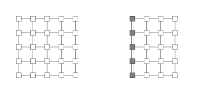
Figure 16: A tensor network which contracts the left most column with the second one.

5.4.2 TN decoding for the planar code

A surface code encodes a single logical qubit, therefore the normalizer cosists of the following logical cosets: $I_{L}$, $X_{L}$, $Y_{L}$ and $Z_{L}$. As a result of degeneracy, the most probable Pauli error corresponding to a syndrome does not need to correspond to the most probable error class for such syndrome [54]. As mentioned earlier, when facing a non-trivial syndrome in a code, a TN decoder will seek to find a Pauli error correspondent to the syndrome, $E_{rec}$, and the most probable logical coset given the chosen error $E_{rec}$. In this sense, the planar code can be associated to a PEPS tensor network [121] following:

$$p(E_{rec}\mathcal{L})=\sum_{\alpha,\beta}T(\alpha;\beta),$$ (20)

where $p(E_{rec}\mathcal{L})$ is the probability of the error being within the error class $\mathcal{L}$ and $\alpha_{i},\beta_{j}\in\{0,1\}$ indicate the application of the stabilizer generator operators. An arbitrary application of a stabilizer element operator would be denoted as $g(\alpha,\beta):=\prod_{i}(A_{i})^{\alpha_{i}}\prod_{j}(B_{j})^{\alpha_{j}}$, where $\alpha_{i}$ indicate $X$-stabilizer operators and $\beta_{j}$ indicate $Z$-stabilizer operators. The resulting tensor network is graphically represented in FIG. 17. Note how now all stabilizer generators are considered as identical while the data qubits are labelled as horizontal (H) or vertical (V). This consideration is equivalent, now, horizontal data qubits are considered to be operated with $Z$-stabilizer operators from top and bottom and $X$-stabilizer operators from left and right, while the opposite happens for vertical data qubits.

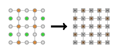
Figure 17: On the left, a distance-3 planar code, on the right the tensor network which represents it. Stabilizer checks are denoted through brown squares and labelled as $s$, and horizontal and vertical data qubits are denoted as $H$ and $V$ respectively.

Under these considerations we can define the tensor nodes which form the overall planar code PEPS tensor network in FIG. 18. The elements of the data qubit tensors are the probabilities of experiencing Pauli errors given by the indices. Moreover, the indices $n$, $e$, $s$ and $w$ indicate the tensors to their north, east, south and west; respectively. The indices are binary and indicate if either of the adjacent stabilizer generators operates non-trivially on them as can be seen in the right side of FIG. 18, where one can see that the state of a data qubit tensor is both dependent on the indices and the correspondent Pauli operator on the qubit from the error $E_{rec}$. On the other side, the stabilizer tensor nodes are defined by Kronecker deltas, i.e. they are either 1 when $n=e=s=w$ and $0$ otherwise. That is because the stabilizer generators either operate on all their nearest data qubits or do not operate on any of them, as was earlier shown in FIG. 2.

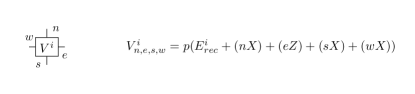
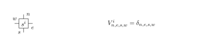
Figure 18: On the left, graphical representation of the tensor nodes which constitute the planar code tensor network. On the right, element values of the tensors, the superindex indicates the labelling of the tensor node.

Since the probability of error of data qubits is independent from one to another, considering an error $E_{rec}$ associated to a syndrome and contracting the tensor network from FIG. 17 results in the summation of products of tensor probabilities under all the combinations of the stabilizer generators, which itself is equivalent to finding the probability of the error class $p(\mathcal{G}E_{rec})$. Unfortunately, and as explained before, contracting columns increases the vertical bond dimension exponentially and, thus, the reasonable approach consists in truncating the vertical bond dimension after each contraction to a truncated value $\chi$. This is often done through the Schmidt decomposition [121, 179], which allows the resulting tensor after the column contraction to be represented as a sum of products of smaller tensors called "Schmidt tensors". The SVD is applied to said Schmidt tensors resulting in the Schmidt values, the truncation follows by only considering the "Schmidt tensors" correspondent to the highest $\chi$ Schmidt values [179]. This allows for obtaining approximate values of the probabilities of the error classes, which can then be used for decoding at a higher precision than any of the aforementioned algorithms, if the truncation of the bond dimension is high enough.

5.4.3 TN decoding for the rotated planar code

For the rotated planar code, the tensor network representation of the system is not as straight forward as in the case of the planar code, since the code can no longer be mapped directly to a PEPS tensor network. An elaborate and efficient way of adapting the TN decoder in [121] for rotated planar codes, while greatly improving their performance was elaborated in [170] as illustrated in FIG. 19. As depicted in the figure, the rotated planar code is first adapted to the tensor network model proposed in [121], which does not correspond to a PEPS state. In order to map such TN to the desired representation, the stabilizer nodes are split in 4 smaller tensor nodes which preserve the delta tensor structure themselves [180], i.e. the values are given by the Kronecker delta. Afterwards, the data qubit nodes altogether with their adjacent stabilizer nodes are contracted producing the desired PEPS. Note how the resulting PEPS is no longer isotropic, i.e. if the PEPS is rotated 45º counter clock-wise, most of the vertical bonds will be of dimension 2 while the horizontal ones will be of dimension 1.

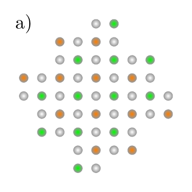
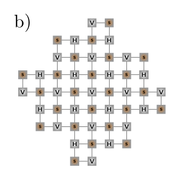
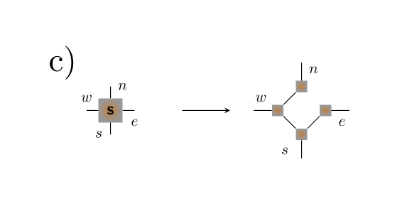
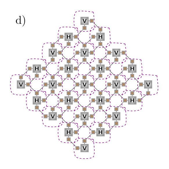
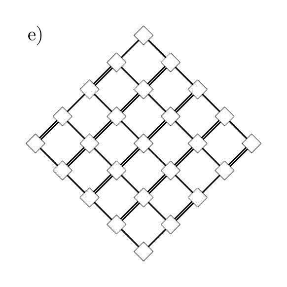
Figure 19: In a), a rotated planar code of distance-5. In b) the tensor network one could extract following [121]. In c), the tensor nodes correspondent to stabilizer generators are split in 4 tensor nodes connected with themselves. In d), a new tensor network arrangement is proposed for the rotated planar code. Notice the tensor network can be separated in sets of tensor nodes which are encircled in dashed violet lines. In e), the aforementioned encircled tensors are contracted and a new tensor network is obtained.

Given this new structure, the rotated planar code can be decoded through the TN decoder. In FIG. 20, we can see an example of the decoding process of an arbitrary syndrome through the TN decoder for a $5\times 5$ rotated planar code. In the top image, the error $E$ is presented altogether with the measured syndrome and in the second image an error $E_{rec}$ which returns the code to the codespace is presented. This error is found by generating chains from every non-trivial syndrome element to its nearest virtual check. Afterwards, the probability cosets of the four logical operators are computed by contracting the associated tensor network. The combination of each of the logical operators with $E_{rec}$ is also presented in the third and fourth row. Finally, the coset with the highest probability is $Y_{L}$ for this example and, thus, the recovered error by the TN decoder is $E_{rec}Y_{L}$. In the figure at the bottom, the resulting state of the code after recovery defined by $E_{rec}Y_{L}E$ can be seen, and, as shown by the highlighted stabilizer operators it belongs to the stabilizer set, implying that the correction has been successful.

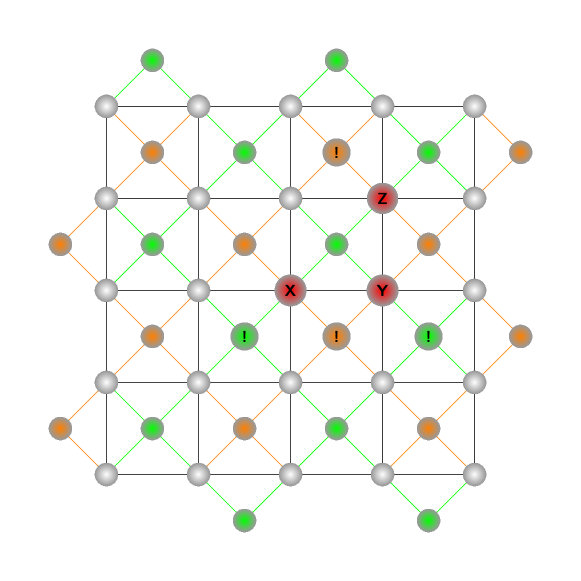
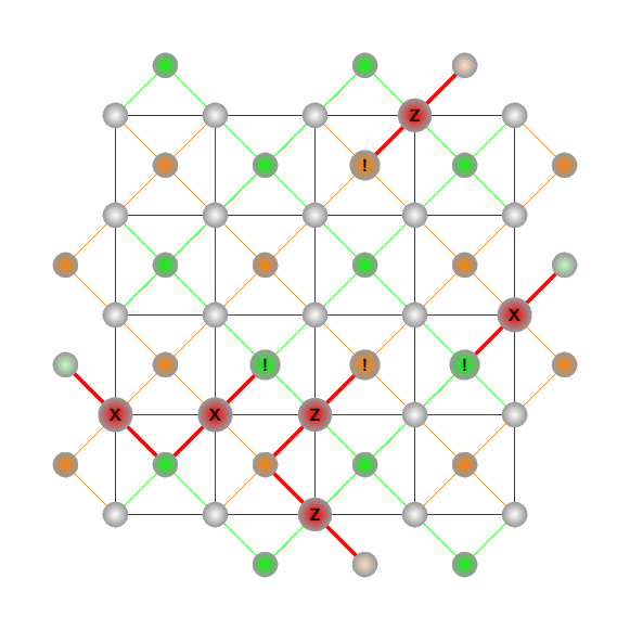
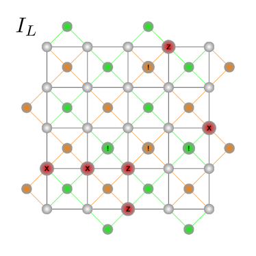
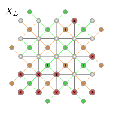
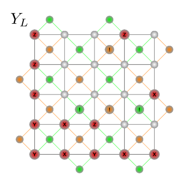
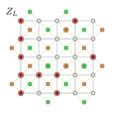
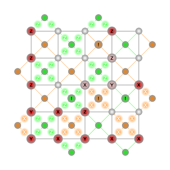
Figure 20: Graphical representation of a TN decoding process for a specific syndrome in a 5x5 surface code.

5.4.4 Performance and threshold

The tensor network decoder has the highest code threshold out of the ones considered in this work equal to $0.185$ under depolarizing noise with a bond dimension $\chi=16$, as can be seen in FIG. 21. It is worth mentioning that this exceptional performance is highly related to the value of $\chi$, the maximum value of which scales in an exponential manner as larger configurations are considered. Recent work has been done studying $\chi$ values for achieving convergence of the tensor network decoding method under several noise model and code tailoring conditions [42, 170].

Moreover, as can be seen in Table 4, tensor network decoding also suffers under biased noise in a significant manner. There have been recent studies which have investigated the effect of biased noise in surface codes and ways to enhance its performance reaching significant results which allowed for lower values of $\chi$ in order to obtain a convergence within the tensor network problem [170, 41]. At the current time, the exceptional performance of the tensor network decoding scheme motivates researchers to seek for methods to accelerate its poor run time.

$\eta$	$p_{th}$
1/2	0.185
1	0.175
10	0.111
100	0.097
1000	0.096

Table 4: Probability threshold values for different biases of the rotated planar code under Pauli noise decoded with the TN decoder with bond dimension $\chi=16$.

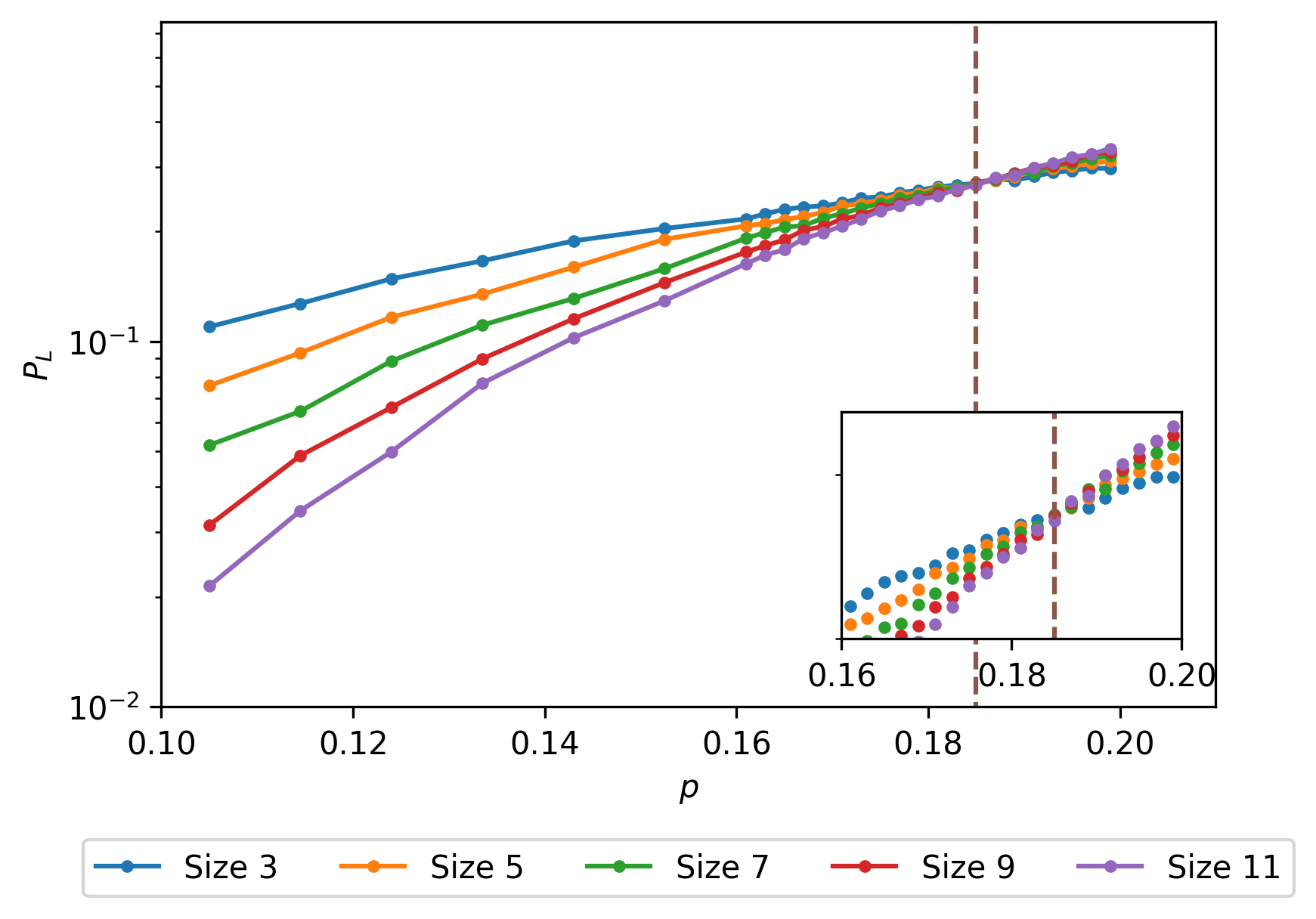
Figure 21: Logical error probability with dependence on the physical error probability of the rotated planar code under depolarizing noise decoded with the TN decoder with bond dimension $\chi=16$.

5.4.5 Complexity

The complexity of the tensor network decoding method is mainly given by two important tasks: the contraction of the MPS with its nearest MPO and the truncation of the resulting state. The contraction of the MPS with the MPO has a complexity of $\mathcal{O}(d\chi^{2})$ while the truncation technique has a complexity $\mathcal{O}(d\chi^{3})$ [121, 181]. Since for every matrix product operation there is a need for $d$ truncation techniques, one for each tensor node within the MPS, the resulting truncation complexity is $\mathcal{O}(d^{2}\chi^{3})=\mathcal{O}(n\chi^{3})$. Thus, the truncation complexity ends up defining the overall complexity of the decoding method.

The resulting complexity is a high price to pay for a DQMLD method, as larger code sizes are considered, the required $\chi$ should be also larger for taking into account the most probable configurations within the stabilizing cosets. The cubic growth with the bond dimension truncation harshly compromises the possible usability of the TN decoder in real-time decoding. Moreover, the Google Quantum AI team observed that this decoder is many orders of magnitude slower than the MWPM implementations used for their experiments [64].

5.4.6 Measurement errors

Considering measurement errors in tensor network decoding is a cumbersome task, since it requires a space-time syndrome extraction which yields additional tensor nodes to take into account. The Google team in [64] studied the tensor network decoding process in a distance-5 code for 25 syndrome extraction rounds by considering a Tanner graph between the syndrome elements and the circuit-level error mechanisms in a similar manner than the method used in [87]. Afterwards, this Tanner graph can be rewritten as a tensor network that evaluates the probability of a logical coset outcome and, it can be planarized and contracted considering a specific truncation [182].

As with the other decoding methods, considering measurement errors significantly increases the complexity of the already complex tensor network decoding method. Nevertheless, the high cost of performing TN decoding allowed for the best performance in the experimental surface code from Google [64].

5.5 Other decoders

Many other decoders have been proposed through the literature for decoding topological codes other than the mainstream MWPM, UF, BPOSD and TN decoders. Many of them have been proposed to decode specific families of topological codes other than the rotated planar code such as the toric or the the color code. In this section we briefly introduce those decoders and discuss their capabilities.

5.5.1 Cellular-automaton decoder

Cellular-automaton decoders were first proposed for decoding the toric code [124]. This class of decoders was constructed with the aim of reducing the decoding problem to simple local update rules in the sense that they only depend on the nearest neighbours. The authors justify that a cellular automaton does fit such requirements and, thus, propose the use of an auxiliary cellular automaton to the toric code such that it communicates long-range information between the non-trivial syndromes that have been with the aim that local decision can be made for correcting the associated error. More specifically, the auxiliary cellular automaton stores real numbers $\phi_{t}(x)$ at each time step, $t$, of the decoder for each of its cells. In this sense, the system depends on the error configuration, the activated syndrome elements at a time step and the value of $\phi$, which includes the values for every cell $x$. In order to update the system state from a time $t$ to the next time step $t+1$, $c$ elementary updates of $\phi$ are done based only on the information of the nearest neighbors and another step where the error and the syndrome on the system at such time step is updated too. For doing so, a nearest syndrome is triggered based on an update rule. By repeating this $\tau$ times, the closest potential partners are found when two syndromes cancel each other, implying that a matching has been found, recovery Pauli operation. The authors in [124] propose that $phi$ represents an attractive force between the measured syndrome, emulating an electrostatic or gravitational field which can be discretized into update rules since they can be discretized to local dynamics. Therefore, they propose to emulate the long field attraction of those fields to represent that the closest triggered syndromes are attracted, and they propose the local dynamics induced by those laws to updated the values locally.

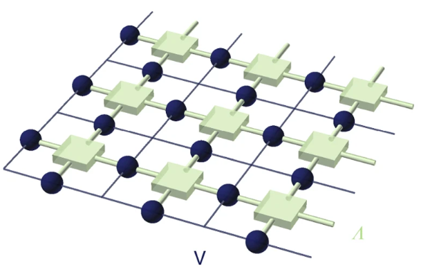
Figure 22: Visual representation of the 2D cellular automaton decoder for the toric code with periodic boundaries. The blue dots, represented by lattice $V$, are the data qubits while the green boxes, represented by lattice $\Lambda$, depict the cellular automaton decoder. Figure taken from [124].

The update rule proposed by the authors is based on selecting which of the neighbour syndromes is activated as a function of the field intensity provided by the values of $\phi$. In this sense, they look for the the adjacent cell with largest field value and then move there with a probability $1/2$. Regarding the function $\phi$, a local discretization of the Gauss’ law was selected for emulating the long field attraction [124]. There have been other proposals for the update rule of the cellular automaton decoder such as the so called Toom’s rule [183, 184] or the sweep rule [185, 186]. Most of the cellular automaton decoders have been studied for toric codes with boundaries in $d$ dimensions [124, 183, 184, 185, 186], but some lattices without boundaries have examined [186]. Additionally, it was shown that the decoders for the toric code can be applied to decode color codes [187] and, thus, cellular automaton decoders can also be applied for this family of QECCs. Unfortunately, its application for a rotated planar code has not been investigated.

Regarding the threshold achieved by this class of decoders it is noteworthy to say that the noise model considered has been primarily an i.i.d. phase flip model [124, 183, 184, 185, 186]. In this sense, a threshold of $8.2\%$ was claimed in [124] for a 2D toric code, while a MWPM decoder exhibits a $10.31\%$ threshold for such code [188]. However, a threshold of $15.5\%$ was claimed in [184] for the cubic toric code using the sweep rule. In terms of the complexity of this decoder, it can naturally be integrated in a parallel way by communicating the processing cores locally and, therefore, it is usually seemed as a fast decoder [124, 185, 186]. In this sense, the 2D cellular automaton of [124] requires a number of updates in the order of $\log^{5}(d)$ updates, while the 3D implementation requires a number of updates in the order of $\log^{3}(d)$. As the authors discuss, this comes from the fact that the cellular automata decoder accepts a parallel implementation from construction [124]. The sweep decoder implementation in [185] requires a runtime $\mathcal{O}(d)$, so linear in $d$.

An important feature of cellular automaton decoders is that they are robust for the case that measurement errors are considered [185, 186]. Specifically, this decoder is deemed to be a single-shot decoder, which implies that measurement errors can be dealt with a single decoding round (recall Appendix B). This is specially interesting for a decoder since as discussed before, the way in which decoders usually deal with noisy syndromes is by performing $d$ measurement rounds and then solving the space-time like obtained graph [186].

5.5.2 Renormalization group decoder

The renormalization group (RG) decoder was proposed as a fast and efficient decoder for the Kitaev toric code [123]. The main idea behind this decoder is that the toric code can be seen as a concatenated code so that the decoding problem can be resolved from the smaller codes that form it. The toric code is not exactly a concatenated code, but the authors propose that it can be actually considered to be one when allowing the blocks of the concatenation to share qubits, so they are actually overlapped [123]. Following this rationale, the RG decoder computes the logical error probabilities of the smallest codes in the concatenation, which then are used as the noise model for the second layer of codes on the concatenation. the process is repeated until reaching the top layer of the code, which actually reperesents the complete toric code and, thus, the estimation of the error is obtained for correction. The authors discuss that since the small codes for the concatenation are small open-boundary topological codes, those can be decoded by brute force [123].

As stated, the renormalization decoder was originally proposed for the Kitaev toric code, so with periodic boundaries, but modifications for decoding color codes [189], the 3D cubic code [190, 191, 192] qudit topological codes [191, 193, 194] and the four-dimensional toric code (both for periodic and open boundary conditions) [195] have also been proposed. Interestingly, the RG decoder was the first known algorithm to decode the color code. The RG decoder has not been investigated for the rotated planar code discussed thorugh this paper, but it could be valid, in principle, by using the ideas for decoding open boundary four-dimensional toric codes [195] since the rotated planar code is essentially a rotated toric code with boundaries.

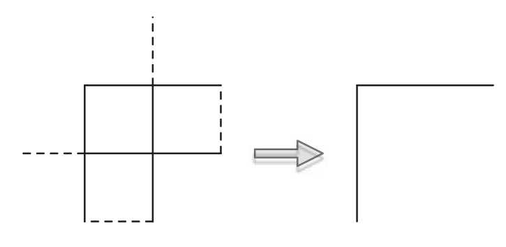
Figure 23: Example of a code block decomposition used for RG decoding. Each of the edges represnt a qubit (12 total). In this example, a subcode of two qubits is used for RG. The dashed lines represent qubits shared by two blocks due to the fact that the toric code is not exactly a concatenated code. Figure taken from [123].

Regarding the code threshold achieved by RG decoders, its standard version shown a threshold of $7.8\%$ for the depolarizing noise model, which falls short when compared to the $15.5\%$ threshold obtained by decoding it with the MWPM decoder. However, the application of belief-propagation decoder before the RG decoder was proposed in [123]. This was done so that the smallest codes of the concatenation can start the decoding with the probability distribution given by BP implying that the RG is more accurate globally. By doing so, the BP+RG decoder achieved a $16.5\%$ threshold, which exceeds that of the MWPM decoder by itself [123]. This, however, was comparing the performance with the MPWM alone, i.e. belief-matching would also increase the threshold [158, 87]. In addition, it does not exceed the threshold achieved by the tensor network decoder, which stands between $17\%$ and $18.5\%$ [121].

Similar to the cellular automata decoder, the RG decoder admits a parallelization of the decoding problem since each of the codes forming a layer of the concatenation can be decoded in at the same time [123]. This implies that the complexity of the algorithm is a function of the number of concatenation layers, which scales logarithmically with the distance and, thus, number of qubits of the code. Therefore, the decoding complexity of the standard RG decoder is in the order of $\mathcal{O}(d)$ if the complete parallelization is done, while in the order of $\mathcal{O}(d^{2}\log{d})$ if the decoding is done serially [123]. Therefore, this decoder is considered to be a fast decoder. The BP+RG approach for increasing the threshold will suffer a toll in the complexity coming from having to execute BP too. It is noteworthy to say that whenever faulty syndrome measurements coming from circuit level noise are considered, the RG decoder needs $d$ rounds of measurements for dealing with them, implying that the complexity of the decoder will also increase [186].

5.5.3 Neural-network decoders

Neural-network (NN) decoders are a result of applying machine learning (ML) techniques for decoding quantum error correction codes [125]. In order to do so, the authors of the NN decoder proposed reducing the decoding problem to the well-studied ML problem of classification, which generally consist on optimizing the assignment of known labels (generally low-dimensional) to known inputs (generally high-dimensional) with the scope of afterwards using the optimized assignment to label inputs that are unknown. A toy example of a classification problem in ML is to label photos of cats and dogs, i.e. to say which photos depict cats and which dogs [196]. The stage in which the classifier is optimized with known data is named training. Hence, NN decoders need a training stage before being able to decode. In the context of the analogy with machine learning, the authors propose to decompose an error into three multi-qubit Pauli operators as $E=STL$, where $S$ is an element of the stabilizer, $T$ is any fixed Pauli that produces the error syndrome (usually referred as pure error) and $L$ is a logical Pauli operator [125]. Note that this decomposition is standard in the field of quantum error correction [54]. Due to the degenerate nature of QECCs, any recovery operator $E^{\prime}=S^{\prime}TL$ will successfully correct the corrupted codeword implying that the stabilizer element of the recovery operator can be assigned arbitrarily with no impact in the logical error rate of the correcting method. In addition, the authors discuss that the pure error can be produced using a parallel table look-up since each element of the error syndrome depends on a unique pure error independently of the others [125]. The algorithms performing such two assignments is named as the simple decoder. Hence, the NN decoder is based on the fact that since the rotated planar code encodes one logical qubit, the logical operators associated are $\mathrm{\hat{I},\hat{X},\hat{Y},\hat{Z}}$ (the hat refers to the fact that those operators are defined over the logical qubit) and, therefore, decoding can be done with as a classification problem with those four labels.

The way in which the classification problem was dealt with in [125] was by using feed-forward neural networks. The neural network in question is defined by a graph consisted of many artificial neuron layers which are connected among them. The neurons are defined by a so called-activation function which depends on an array of weights, $\bar{w}$, of length $m$ and a bias $b$. Since the NN is of the feed forward type, the neurons calculate the nonlinear activation function ($\bar{x}$ is the input and $*$ refers to the inner product), $\bar{y}=(1+\mathrm{exp}(-(\bar{w}*\bar{x}+b)))^{-1}$, and pass it to the subsequent layer until the output layer is reached, where the result of the activation function is rounded to $\{0,1\}$ so that the output of the algorithm is obtained [125]. The layers between the input and output layers are named as hidden layers in the terminology of ML. As explained before, a neural network requires a training stage before it can operate over a set of unknown data. Therefore, for the NN decoder, a training stage where the weights and biases of the neurons are trained is needed. The authors of [125] select the average cross-entropy as the cost function to optimize the activation function and produce a training set directly sampling errors at an error probability where the MWPM decoder has a $25\%$ logical error rate. The cost-function was minimized by stochastic gradient descent, while the number of elements of the training set was limited to at most $10^{6}$ samples.

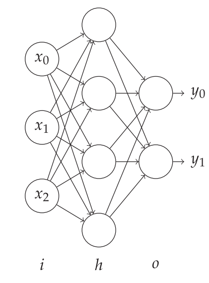
Figure 24: Graphical depiction of the feed-forward neural network used for the NN decoder. The example consists of an input layer (i), a hidden layer (h) and an output layer (o). The inputs represent the syndrome data, while the outputs refer to the estimated logical error. Each of the neurons in every layer compute the activation function as a function of their received information and pass the information to the next layer. Figure taken from [125].

The NN decoder in [125] proved to be an efficient method for decoding small distance, $d\in\{3,5,7\}$, rotated planar codes achieving similar performance as the MWPM decoder while maintaining a similar complexity. As a result of the interesting performance of this decoder, several studies discussing ML decoders for the rotated planar code have been proposed such as the deep neural network based decoder in [197, 198] or the reinforcement learning based decoder in [199]. The deep neural network decoder proved a better threshold than MWPM at the cost of a higher complexity, while the reinforcement learning decoder proved an almost linear complexity at the cost of a worse code threshold [198]. Combinations of NN decoders with RG decoders have also been proposed [200]. Recently, NN decoding methods for surface codes that do not rely on an specific error model, i.e. that are purely based on hardware obtained data, have been proposed [201, 202]. Machine learning based decoding methods have also been proposed for other topological codes such as the toric code [203, 204, 205, 206, 207, 208, 209, 210, 211], the color code [212] or the semionic code [213]. Each of the proposed ML decoders for each of the codes provide either a faster decoding or a better threshold than other methods, showing the natural trade-off between accuracy and speed.

Circuit level noise has also been considered for neural network decoders, i.e. faulty syndrome data arising from noisy gates and measurements [125, 197, 212, 214]. In a similar fashion as other decoders, dealing with noisy measurements requires approximately $d$ syndrome measurement rounds, implying that the runtime of the decoders increases. Importantly, NN decoder should be trained using this error model so that they can cope with it, i.e. training is specific to the noise model in consideration [125]. The performance of the NN decoder of [125] achieves the same performance as MWPM for this scenario.

To sum up, NN decoders are promising in the quest of obtaining accurate and fast decoders for decoding not only rotated planar codes but also other families of error correcting codes. Some of the problematic behind this family of decoders is the training cost, which may scale exponentially with the code distance [186]. This is one of the main reasons behind the fact that most of the NN-based decoders have only been tested for small distances $d<10$ [211]. Interestingly, promising results have been obtained for decoding the toric code with an NN+UF decoder that achieves high threshold with almost linear complexity, while having been tested up to $d=255$ [211]. However, the need of a training stage before operation implies that NN and ML decoders might not be the best choice when the noise fluctuates over time, as it occurs for superconducting qubit platforms [35, 133]. Additionally, it is important to state that mapping the decoding problem to a ML classification problem works well for the rotated planar code or other topological codes since they encode a low number of logical qubits, implying that the possible logical errors is not too high. However, since the number of logical errors scales as $2^{2k}$ with the number of logical qubits [128], $k$, these methods may not be implementable for other families of codes with higher coding rates such as QLDPC codes.

5.5.4 MaxSAT decoder

The MaxSAT decoder has been recently proposed as an efficient algorithm to decode color codes [126]. This decoder is based on the analogy between the decoding problem of the color code and the LightsOut puzzle when the error model in consideration is the bit-flip noise. The LightsOut puzzle refers to a problem where a lattice whose faces are associated with switches and lights can be either on or off. In such lattice, toggling a switch on the lattice implies that all its neighbouring lights change their previous state, i.e. if they were on they are turned of and vice versa. The LightsOut problem then tries to find out a sequence of switch actions so that all lights are turned off. The puzzle has two important properties: toggling a switch twice is the same as not doing anything and the state of a light only depends on how often its neighbour switch have been toggled (independence on the order). The authors argue that this problem is similar to the decoding process of a color code by doing the following analogy:

• Data qubits $\leftrightarrow$ switches.

• Checks $\leftrightarrow$ lights.

• Syndrome $\leftrightarrow$ initial light configuration.

• Decoding estimate $\leftrightarrow$ switch set that is a solution.

• Minimum-weight decoding estimate $\leftrightarrow$ solution with minimum switch operations.

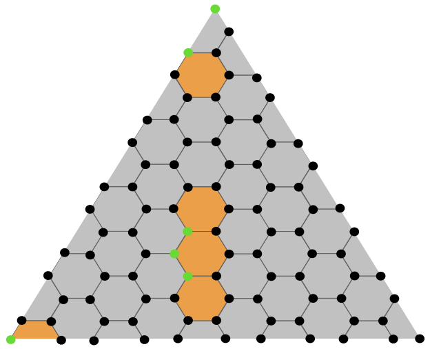
Figure 25: LightsOut and color code ($d=11$) decoding analogy. The marked faces represent the initial configuration (syndrome), while the green data qubits represent a possible solution of the problem which is not necessarily minimal. Figure taken from [126].

Therefore, the authors exploit such an analogy to propose a decoding methods based on solving the LightsOut puzzle. The main idea is to find the minimal solution set for the puzzle, which is equivalent to a decoding estimate of minimum weight matching the syndrome measurement. In order to obtain the minimal solution of the LightsOut puzzle, the authors formulate such problem as a maximum satisfiability (MaxSAT) problem, which generally refers to the problem of determining the maximum number of clauses of a Boolean function that can be made true by assigning true values to the variables [215]. Following this rationale, the authors formulate the decoding problem as the MaxSAT problem

$$\begin{split}\forall f\in F:&\bigoplus_{v\in\mathcal{F}_{\mathrm{switches}}(f)}\mathrm{switch}_{v}=\mathcal{F}_{\mathrm{init}}(f),\\ &\forall f\in F:\mathrm{not}(\mathrm{switch}_{f}),\end{split}$$ (21)

where $f\in F$ refer to the lights or faces, the $\mathrm{switch}_{v}$ are Boolean variables representing if a switch is toggled, $\mathcal{F}_{\mathrm{switches}}(f)$ is a discrete function that takes a face $f$ and returns the set of switches surrounding it; and $\mathcal{F}_{\mathrm{init}}$ is a Boolean function that describes the initial configuration of the system (associated with the measured syndrome). $\bigoplus$ denotes the exclusive-or (XOR) Boolean operation. In equation (21), the constraints in the first line represent the satisfiability problem, and the second are the soft constraints so that such problem is maximum. Hence, color code decoding can be done by solving such MaxSAT problem [126]. The authors discuss many MaxSAT solvers for decoding the color code.

The MaxSAT decoder for bit-flip error noise in color codes was proven to have a very high threshold of $10.1\%$ [126]. This is near the optimal $10.9\%$ threshold obtained by the MPS or TN decoder, and substantially exceed the $\approx 9\%$ of the MWPM, $8\%$ of the Uf and $7.8\%$ of the RG decoders. This excellent threshold does not come free of charge since it implies a higher decoding runtime. The authors do not discuss the complexity of the MaxSAT decoder, but they do explain that the runtime is slower than the ones of MWPM, UF and RG decoders, while it is faster than the TN decoder. This is consistent with the typical performances versus complexity trade-off discussed throughout this tutorial. The toll in runtime comes from the fact that the MaxSAT problem is an NP-hard problem [126]. Importantly, the authors argue that the MaxSAT decoder is faster whenever the physical error rate is lower, which is a desired feature as QECCs are expected to be working in sub-threshold noise levels.

In conclusion, the MaxSAT decoder is an efficient decoding method for the color code that exhibits a very high code threshold for bit-flip noise with a more reasonable complexity when compared with the tensor network decoder. However, at the time of writing, the MaxSAT decode is yet a limited approach, mainly due to the fact that only bit-flip noise is considered. This is very important since the LightsOut analogy proposed by the authors in [126] depends on such error model assumption. Additionally, no faulty measurements have been considered and it is rather unclear if the decoder will be able to operate whenever circuit noise level is considered. Nevertheless, this decoding method has been very recently proposed and generalizations of it for noises with other structures (importantly the depolarizing channel) and other families of topological codes can be expected as future work.

5.6 Software Packages

In this section an overview regarding the existing software packages for surface code decoding simulation will be covered. Fortunately, the scientific community has provided a large number of open source repositories for performing simulations of several decoders of the surface code and other topological codes and, thus, we will cover several of them (the most popular and used ones) as a reference for people on the community of quantum error correction. We provide a graphical overview in FIG. 26.

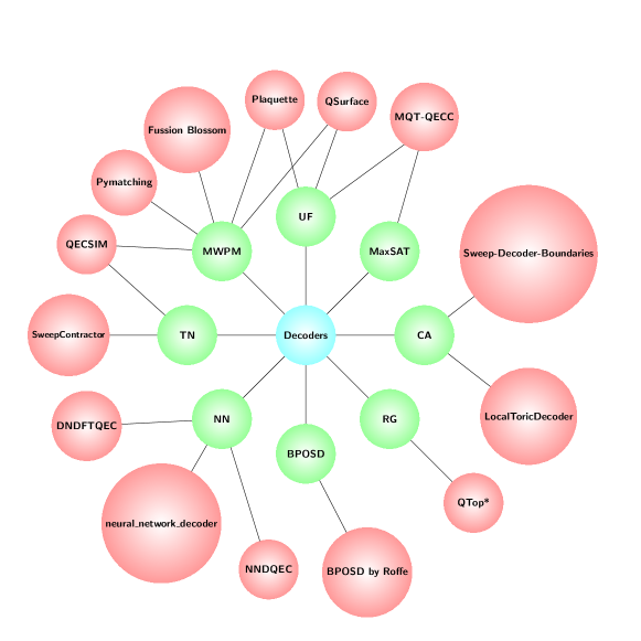
Figure 26: Sketch representing the available software packages for each mentioned decoder. Each edge connects each decoder (green circle), with the software packages which support it (pink circles). The decoders mentioned in the figure are the Cellular Automata decoder (CA), the MaxSAT decoder, the Union Find decoder (UF), the Minimum Weight Perfect Matching decoder (MWPM), the Tensor Network decoder (TN) the Neural Network decoder (NN), the Belief Propagation + Order Statistics Decoder (BPOSD) and the Renormalized Group decoder (RG).

Whenever considering numerical simulations of a surface code, it is important to be able to generate the samples of the noise following the distribution of interest for a certain scenario so that the decoder operates over such noise model. In this sense, generating samples for data qubit noise is pretty straightforward by considering the specific distribution of the Pauli channel for each of the qubits (See section 4). Nevertheless, whenever circuit-level noise for faulty check measuments is considered, sampling the noise is not a trivial task [136]. Therefore, the Stim repository by Craig Gidney was developed for sampling circuit-level noise for the sake of obtaining samples of noise that accurately resemble the errors that a surface code experiences over such scenario [136]. Stim samples circuit noise to all qubits within the code, including measurement qubits, at a fast speed and is the simulator of choice when considering stabilizing circuit noise. This repository can analyze a $d=100$ surface code circuits in approximately 15 seconds for sampling circuit shots at a rate of 1000 samples per second.

Regarding software implementations of the minimum weight perfect matching decoder there are several open source repositories which successfully simulate realizations of the decoder at a sufficient speed. The most popular and quickest one considering serial computation is Oscar Higgot’s the Pymatching repository [57, 120], the latest version of which, implements the Sparse Blossom implementation of the MWPM decoder. The Fusion Blossom algorithm [119] is also available at the GitHub repository by Yue Wu [118] which, as explained before, albeit having a worse serial performance than Pymatching, allows parallel decoding improving the complexity at each additional node and eventually surpassing the performance of Pymatching. Additionally, the QECSIM repository by David Tuckett [180] also stands as a fair simulator for the minimum weight perfect matching which also allows other decoding methods. Another recent software package that incorporates Pymatching and Fusion Blossom (by calling those repositories) was posted in the Plaquette repository by the QC Design team [216]. Interestingly, such repository incorporates Stim too, allowing the combination of all those repositories in a single one.

An implementation of the UF decoder can be found in the Qsurface [217]. The package allows the simulation of the standard union-find decoder [109] as well as a modification of it by the authors of Qsurface which they name as Union-find Node-Suspension decoder. The authors claim that an improved threshold can be obtained by using such modified decoder while maintaining complexity. Moreover, such package includes an implementation of the MWPM algorithm. The previously discussed Plaquette package [216] also includes an implementation of the UF decoder by Delfosse and Nickerson. The inclusion of this decoder is specially interesting for the Plaquette package since the circuit-level noise obtained from Stim can be directly used for testing the UF decoder.

The BPOSD algorithm was originally thought as a general decoder for QLDPC codes [46]. However, a surface code can be seen as a sparse code as the distance of the code increases (due to the fact that the weight of the stabilizer is constant independently of the size). In this sense, the BP+OSD: A decoder for quantum LDPC codes package by Joschka Roffe [218] implements the BPOSD decoder for general QLDPC codes. For simulating surface codes, the parity check matrix [30] of such code should be used whenever defining the QLDPC code to be decoded by the BPOSD implementation.

The aforementioned QECSIM repository [180] does also include an implementation of the tensor network decoder. The package include the possibility of tuning the truncation parameter that is used for the TN decoder. Another implementation of the tensor network decoder can be found in the SweepContractor repository by Cristopher Chubb [219] which is based in the sweep line algorithm of [171].

In the case of cellular automaton decoders, the repository Sweep-Decoder-Boundaries by Michael Vasmer [220] implements the version of the decoder using the sweep rule as presented in [185, 186]. As discussed in the papers, the implementation of the decoder admits simulations using circuit-level noise. Additionally, the repository LocalToricDecoder by Kasper Duivenvoorden implements the version of the cellular automaton using Toom’s rule as proposed in [183, 184]. We have been unable to find software packages implementing the other cellular automaton decoders discussed.

Concerning the RG decoder, the QTop repository by Jacob Marks [221] presents an implementation of it. However, it is noteworthy to say that the author stated in the repository that such software package is not being actively maintained and, thus, it may be unreliable. Anyway, the code is available there for anyone that may be interested in testing it or using it to code its own version of RG decoders.

With respect to neural network decoders, the repository Neural Network Decoders for Quantum Error Correcting Codes by Stefan Krastanov [222] implements the neural network decoder proposed in [204] for the toric code. Moreover, Pooya Ronagh developed a the repository Deep Neural Decoders for Fault-Tolerant Quantum Error Correction [223] for the deep neural network decoder proposed in [197] for decoding rotated planar codes. Interestingly, the authors of both repositories programmed the decoders so that other neural networks than the ones in [204, 197] can be incorporated. Hence, those repositories provide freedom to integrate other neural network decoders of the literature. Finally, the repository neural_network_decoder by Paul Baireuther [224]contains the implementation of the neural network decoder for the color code in [212].

To finish with this section, there is a repository with the implementation of the MaxSAT decoder presented in [126]. The repository, developed at the Technical University of Munich, is named QECC: An MQT tool for Quantum Error Correcting Codes written in C++ [225] and is intended to be a more general tool for QEC than just the MaxSAT decoder for color codes. At the time of writing, the authors of the repository state that the project is still in early development and, thus, will contain other QEC software tools. The main ideas used for the software package were presented in [226]. Either way, at the moment of writing, the MaxSAT decoder and a decoder for QLDPCs based on the UF decoder [140] are present in the software package. Note that since surface codes can be seen as QLDPC codes, the UF decoder implemented in [225] can in principle be used to decode such families of codes.

6 Discussion

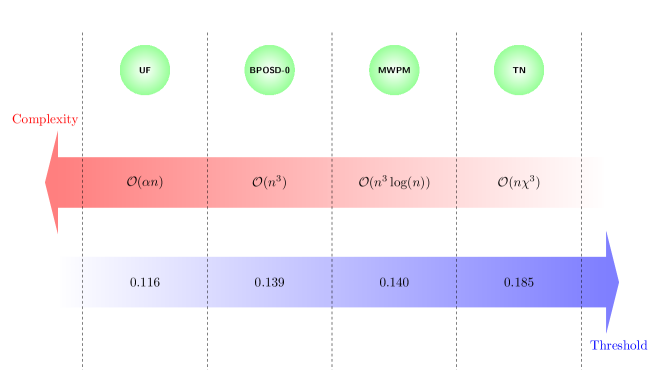
Figure 27: Graphical illustration showcasing the complexity and probability threshold of the decoders studied in this work. This comparative figure is inspired by a figure in [126].

The construction of a fault-tolerant quantum computer remains as the Holy Grail of quantum computing so that the groundbreaking theoretical potential of such technology can be achieved. The key element to solve this quandary is quantum error correction. Quantum information has proven to be so frail that the scientific community has accepted that quantum computing will be unrealizable without QEC. One of the principal elements of a QECC is the decoder, or the classical algorithm that is used to estimate which error has corrupted the quantum information. Due to the urgent necessity of obtaining fast and accurate enough decoders that can operate in real-time for experimentally implemented QECCs, the number of papers related to this is increasing in a very fast pace. In this sense, the QEC community is strongly pushing the state-of-the-art of the topic so that fault-tolerance can be a reality as fast as possible.

As presented in the main text, the main decoders for the rotated planar code family are the MWPM, UF, BPOSD and TN decoders. FIG. 27 is an illustrative representation of the accuracy versus runtime trade-off discussed through the text for those decoders. At the time of writing, it seems that the MWPM is an strong candidate due to its high threshold and the fact that it always returns the $X$ and $Z$-errors of minimum weight matching the observed syndrome. In addition, the MWPM decoder presents a considerable worst-case complexity when compared to other decoding methods, but recent implementations of the algorithm have proven to present an almost linear expected complexity [57, 119], making this method even more powerful yet. On the other hand, UF also stands as a fair contestant due to its decoding speed which comes from a linear worst-case complexity. Nevertheless, as discussed before, the MWPM implementations with an average complexity lower than $\mathcal{O}(n^{2})$ [57], even reaching linearity given that enough nodes for parallelization are available [119], make the candidacy of the UF decoder to significantly lose strength. Anyway, it is noteworthy to state that many of those fast MWPM implementations were constructed based on many ideas introduced by UF decoding. The BPOSD-0 decoder lays in a middle ground between the MWPM and UF decoders whenever the rotated planar code is considered. As discussed before, increasing the search depth of the OSD algoirthm has a considerable impact on the worst-case complexity of the decoder and, thus, the benefits of this decoder will probably be lost due to the fact that the threshold of the code would not increase as much. In this sense, it seems that the MWPM decoder is a better candidate for the specific instance of surface codes. Nonetheless, the BPOSD algorithm was proposed as a general decoder for QLDPC codes [46] and, therefore, it is the best candidate for decoding such family of codes which is being studied thoroughly at the time of writing. As seen in the earlier section, its implementation allows the circumnavigation of split beliefs in conventional belief propagation decoding, which have posed a great hurdle to conventional BP decoding for QLDPC codes [150, 46]. The TN decoder achieves the highest code threshold for the rotated planar code, albeit at the expense of the largest worst-case computational complexity. Both the benefit and drawback of this algorithm is a result of the fact that it is an effort to solve the maximum-likelihood (ML) problem explicitly, and this is why it is usually referred as the ML decoder. In this sense, the TN decoder is an almost brute force approach where such brute force search is limited by the bond dimension, $\chi$, which is the approximation parameter that is needed for this method to be actually implementable for codes of considerable size. Hence, the bond dimension is the parameter that will be in charge of the accuracy and speed of the algorithm. Due to the enormous growth in bond dimension in the surface code tensor network contraction, the tensor network is not really considered for real-time decoding but is studied cautiously as an effective degenerate quantum maximum likelihood decoder. Also this decoder presents the possibility of the experimental implementation of codes beyond break-even with poorer hardware capabilities due to its high threshold. The conclusion to this is that the choice of the decoder for a future real-time implementation of surface codes remains as an open question. This quandary is even more complex taking into account the existence of other decoding approaches such as the CA, RG, NN or MaxSAT decoders discussed in this tutotrial. Each of those may provide interesting features that may be beneficial for specific families of codes or even adaptations of them may be interesting for the context of rotated planar codes. For example, machine learning base decoders are gaining popularity on the recent times, probably due to the huge interest in machine learning in general.

In this line, recent breakthroughs have been achieved in the experimental implementations of surface codes over superconducting qubit platforms [63, 64]. Both of the experimental implementations were based on the rotated planar code discussed throughout this tutorial. In [63], Andreas Wallraff’s group at ETH Zurich led an experiment based on the rotated planar code of distance three by means of a processor consisted of 17 transmon qubits. Krinner et al. used the obtained data after multiple measurement rounds in order to run the MWPM decoder for estimating the errors corrupting the quantum information. In [64], the Google Quantum AI realized an experiment based on the rotated planar codes of distances 3 and 5 by means of their expanded Sycamore device consisted of 72 transmon qubits. The authors actually run experiments for the distance-5 rotated planar codes since the actual data for the distance-3 code can be obtained from such code. Acharya et al. used the obatined data to decode the errors by means of the TN and belief-matching decoders. In this way, the authors proved that the logical error rate obtained by the rotated planar code improved as the distance of the code increased for both decoders. This result is really important since the code was operating in a sub-threshold noise level and it represents an experimental proof that the performance of the codes can be increased by increasing the distance (recall the threshold theorem). Importantly, both of the experiments performed the execution of the decoding algorithm by dealing with the measured data in a post-processing stage, i.e. no real-time decoding was actually performed. However, both of these experiments represent the state-of-the-art of experimental implementations of surface codes and they are an effort to progress towards the ultimate goal of fault-tolerant quantum computes.

Following the present discussion, and as it has been seen throughout the text, the decoding stage stands as a pivotal operation within the successful functioning of, not only the surface code, but any correcting code in general. One should be aware of the fact that the named code threshold depends on three aspects: the code family in consideration, the decoding method for the code and the noise model in consideration [90, 91]. In this sense, it is straightforward to see that designing decoding algorithms is crucial in terms of the ability of a family of codes to correct errors. The intrinsic locality and degeneracy of the surface code allows for several decoding processes to present themselves as valid candidates for future real device implementation. Nevertheless, in addition to the code threshold for a decoding method, two other critical aspects stand as limiting factors for the implementation of surface codes decoding in a real-time fashion when implemented on experimental hardware: run time and circuit-level noise.

Decoding runtime refers to the actual time that a decoder requires to ouptut an estimate of the error that has corrupted the logical qubit encoded by a code. Hence, this inherently imposes a delay in the error correcting system that is hazardous for its actual operation. This comes from the fact that, once the syndrome measurement has been done, the data qubits will still continue to suffer from errors as they will not stop to decohere. Thus, if the delay between measuring the checks and applying the recovery operation is too high, then the algorithm will fail, with high probability, the actual error configuration when recovery is executed (See appendix A for a discussion of why real-time decoding is required). This is especially important by taking into account that the decoherence times of state-of-the-art qubits are short and the generation of syndrome data is done a fast rate [30]. As seen in through this tutorial, it is pretty fair to state that maintaining code threshold while reducing the actual complexity of a decoder is a hard problem. This is a result of the trade-off of being fast against considering more error configurations, which actually relates to code performance. This logic comes from the fact that the traditional comparison of accurate and fast is done in terms of code threshold and worst case complexity. However, it is a recent trend to benchmark runtime by expected complexity, i.e. an average of the number of operation required to decode different error patterns. The rationale behind this is that worst-case events are generally exponentially rare, implying that their impact will not be as high in code performance as other more frequent cases. This effect should be more important whenever hardware noise improves lower to sub-threshold physical error rates and, thus, expected runtime might be a better benchmark for decoding algorithms. In this sense, designing faster decoding algorithms that are able to maintain the capabilities of the code in terms of decoding accuracy is a critical issue for the QEC field. It is important to state that significant advances in this direction are being obtained with proposals such as Sparse Blossom [57] or Fussion Blossom [119]. Furthermore, recently, sliding-window decoding schemes have been proposed that allow parallel decoding of the syndrome data by means of matching like decoding algorithms (MWPM and UF), thus, dealing with the exponential backlog problem of real-time decoding while maintaining logical fidelity [227, 228].

On the other side, considering circuit-level noise is fundamental so that surface codes are successful when implemented in real hardware. As explained before, the consequence of such noise associated to imperfect gates, SPAM and error propagation results in measurement errors that make the decoder not to be able to correctly estimate the actual error that has corrupted the data qubits of code (refer to Section 4). In this sense, considering circuit-level noise is sometimes referred as fault-tolerant error models as it is considering all the errors of the elements of the system [125]. Circuit-level noise is usually alleviated by means of multiple measurement rounds, in the order of $\mathcal{O}(d)$, so that the additional errors that led to measurement errors can be taken into account for the decoding problem (refer to Appendix B for a more detailed description). Nevertheless, such multi-round measurement results in a toll for complexity and, hence, runtime. This directly hinders the previously discussed necessity of being fast in decoding so that error correction is successful. Additionally, even when the multiple measurement protocol is applied, the code threshold significantly decreases (usually an order of magnitude) in comparison to thresholds that only consider data qubit noise [87, 32]. The direct result of this is that hardware requirements for sub-threshold code implementation become even more stringent. Therefore, circuit-level noise adds another layer of complexity to the already difficult decoding implementation in real hardware. In this sense, improving gate fidelities and decoherence parameters, as well a other noise sources, of state-of-the-art quantum processors will be a very important for obtaining fault-tolerant quantum computers.

Moreover, tailoring both codes and decoders to the specific structure of the noise that the qubits experience is being investigated so that the actual correcting performance for such noise. A widespread example of this is the bias towards $Z$-errors that many state of the art qubit technologies such as silicon spin qubits or ion traps exhibit [30, 229]. As described in section 4, this comes from the fact that the dephasing time, $T_{2}$, of such qubits is much smaller than the energy relaxation time, $T_{1}$. As previously discussed, running the aforementioned decoders over biased noise models usually contributes to a worse threshold than for the depolarizing channel. This, however, occurs due to the fact that the code/decoder is not tailored to work over noise exhibiting such tendency. Specifically, since $X$ and $Z$-errors are decoded independently, then one of the decoding problems results to be more dense if the noise is biased, i.e. it will experience errors with higher weight more probably, and, thus, the actual threshold will be lower since such decoding sub-problem will fail more often. In this sense, the community has actually studied how to deal with some of those noise structures so that performance is maintained or even enhanced. Some examples include:

• The rectangular surface code: using a surface code with rectangular shape makes the minimal weight logical error $Z_{L}$ to require more physical $Z$ operators, increasing the $Z$-distance $d_{Z}$ and, consequently, increasing the number of $Z$-errors it can correct: $(d_{Z}-1)/2$ [131]. On the negative side, this is at the expense of increasing the number of necessary data qubits to $d_{X}d_{Z}$. In FIG. 28, a rectangular code of distances $d_{X}=5,d_{Z}=7$ is shown, notice how the logical operator $Z_{L}$ requires additional Pauli operators than for the $X_{L}$ operator. This code construction may use the reviewed decoders in order to estimate the channel errors.

  

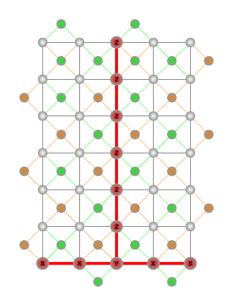
  Figure 28: Graphical representation of a $d_{X}=5,d_{Z}=7$ rectangular rotated planar code. $X_{L}$ and $Z_{L}$ operators are also represented.

• Clifford deformation: in Clifford deformed surface codes, the check qubits are conjugated respect to a unitary operator from the Clifford group [230] so that other valid stabilizers are obtained [106]. By means of this stabilizer modifications, the new stabilizer codes can be constructed so that they are more susceptible to $Z$-noise. For example, the XY-code is a surface code which, instead of having $X$- and $Z$-checks, has $Y$- and $X$-checks, both of which are susceptible to $Z$-noise. A graphical depiction of the XY-code is given in the top figure of FIG. 29. As a result of such susceptibility to $Z$-errors, the associated decoder can make use of the correlation between $X$ and $Y$-errors, i.e. $XY=Z$, in order to be more accurate in detecting $Z$-noise [170, 87, 88]. Another popular Clifford deformed surface code is the XZZX surface code [41, 231]. For this code, all check qubits act equally on their surrounding data qubits operating two $X$ and two $Z$ operators as shown in the bottom figure of FIG. 29. One can see that the commutation between the checks is maintained, since adjacent checks either anti-commute twice or directly commute. An interesting characteristic of the XZZX code is that there is only one set of $Z$ physical operators which produce a logical operator. As is shown in FIG. 29, all the products of this logical operator with the stabilizer set produce physical operators which are composed of $X$, $Y$ and $Z$-operators. This feature complicates the probability of a logical phase-flip, $Z_{L}$, error under a highly $Z$-biased noise model. Moreover, for the case in which the $Z$-bias is infinite, e.g. a pure dephasing channel, the XZZX surface code operates as a series of disjoint repetition codes that can be decoded independently. The data qubits of such repetition codes are the top-left to bottom-right diagonals of the overall XZZX code, as can be seen in the bottom of FIG. 29, where the diagonal consisting of two $Z$ physical errors produces syndromes in their top-left and bottom-right sides. Given this condition, the threshold of the XZZX code reaches an outstanding $50\%$ [41, 231], while reducing the amount of required qubits significantly. Therefore, it can be seen that a bias towards $Z$-errors is not only not problematic, but also beneficial if the code and decoder are tailored for such model.

  

  

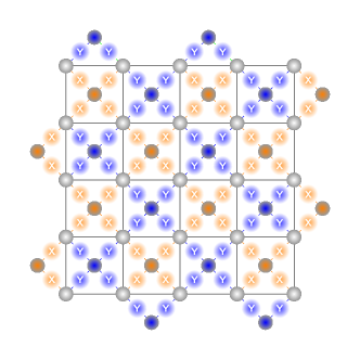
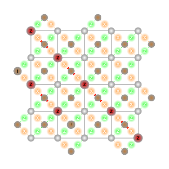
  Figure 29: On the top, a graphical representation of a rotated planar XY code with the operators of the stabilizer generators. On the bottom, the same representation but for the rotated planar XZZX code altogether with a $Z_{L}$ operator

• $X/Z$ correlation: another important approach to improve the performance of surface codes is to make decoders aware of the fact that $Y$-errors represent a correlation between the $X$ and $Z$ errors. One downside of the independent $X$ and $Z$ decoding of CSS codes such as the surface code is that it makes the decoding blind of the correlation among those errors, i.e. it is usually considered that $p_{Y}=p_{X}p_{Z}$. However, as seen in Section 4, the Pauli noise models have $p_{X}\approx p_{Y}$ (both in biased and depolarizing) and, thus, by not taking this into account the decoder underestimates the frequency in which $Y$-errors corrupt the data qubits of the code. A method in order to circumvent this problem (without explicitly changing the structure of the code) consists in first decoding for one of the errors and, afterwards, using the partial recovered error in order to decode the other error. E.g., given an error in a CSS surface code, first decode the $X$-error, and then consider that, for recovering for the $Z$-error, every qubit has an updated probability of undergoing a $Z$-error defined by:

  $$\begin{split}&P(Z|X=1)=\frac{p_{Y}}{p_{X}+p_{Y}}\\ &P(Z|X=0)=p_{Z},\end{split}$$ (22)

  where, $P(Z|X=1)$ is the probability that a specific data qubit undergoes a phase-flip $Z$ given that it has been considered to undergo a bit-flip $X$, and $P(Z|X=0)$ is the probability that a qubit which is considered to not have undergone a bit-flip has undergone a phase-flip $Z$. This can be done once [134, 135, 87] or in a recursive manner [88, 232]. Moreover, it can be combined with the XY-code in order to enhance the susceptibility of the code towards $Z$-noise [87, 88].

Thus, it is important from the decoding (and code construction point of view) to consider the actual noise that the qubits of the surface code experience. As seen for the XZZX code, this tailoring does actually even significantly improve the code performance without needing to lose resources. Even if we have discussed noise bias here, there are many other important subtleties in the nature of the noise for each qubits technology that should be considered for integration in real hardware. For example, multi-qubit error correlation and time-varying noise are examples of this. The fact that the actual distribution of the errors in a real quantum processor is independent seems to be generally false. In this sense, studying the correlated nature of noise is an incipient sub-field in the topic and, thus, tailoring decoding to such correlated nature should improve the performance of the codes over such models [105]. Note that this quandary is not new for classical error correction [233], implying that many ideas of dealing with such noise can be extrapolated to the quantum domain. Modifications of decoders to take into account correlated noise have been already proposed for quantum turbo codes over channels with memory, resulting in a considerably improved performance of the code when compared to the decoder that is blind to the correlation [234]. Additionally, the noise experienced by superconducting qubits has been proven to be time-varying [35, 133], which implies that the performance of the codes experiences a degradation. In this sense, studying adaptive decoders that can estimate the noise level [235] at a certain time in order to follow such fluctuating nature of the noise should considerably improve the performance [236].

To conclude, quantum error correction is still in a primitive stage before the potential of quantum computing can be unleashed by fault-tolerant machines. In this sense, surface codes represent the most promising family of codes to be implemented in the early post-NISQ era, principally due to their locality feature (and, in the case of planar instances, two-dimensional qubit placing) and their high tolerance to quantum noise. As extensively reviewed in this article, decoders represent a central part of QEC methods as they are key elements in posing a threshold for a code. Moreover, we have discussed the importance of the runtime of this algorithms due to the accumulation of other errors if the estimation of the channel error results to be too slow. As a result of this, there exists an important trade-off between accuracy and speed of decoders which implies that a selection of a decoder for real-time decoding depends on many factors that go from the hardware noise level to the pace at which more errors accumulate. Hence, the selection of the best decoder for an experimental implementation of a surface code is still an open question that many research teams, both in academia and industry, are trying to resolve. Due to the extense zoo of possible qubit technologies being investigated nowadays, it is possible that many of the exisitng candidates, or new ones, are the best fit as a function of the specifics of each of the quantum computing platforms. There is much work left to do, and each of us on the field should contribute our share in this Herculean quest. We live in exciting times.

Data availability

The data that supports the findings of this study is available from the corresponding authors upon reasonable request.

Competing Interests

The authors declare no competing interests.

Appendices

Appendix A The backlog problem and why QEC requires real-time decoding

As discussed in the main text, the decoding algorithms for the surface code need to be fast enough to operate in real time. This is necessary because running fault-tolerant algorithms outside the reach of classical simulation requires the use of quantum algorithms that apply $T=\text{diag}(1,e^{i\frac{\pi}{4}})$ gates over the logical space of the code. The use of $T$ gates guarantees that the code supports the universal gate set Clifford+T that can be used to compile any quantum computation, a result known from the Solovay-Kitaev theorem [237]. However, the Eastin-Knill theorem states that no quantum error correction code can implement a universal gate set in a transversal manner . In this regard, the surface code supports transversal implementation of logical Clifford gates but lacks a transversal version of the logical $T$-gate. Fortunately, there are ways to circumvent the Eastin-Knill theorem with the purpose of achieving universal fault-tolerant computation. The most popular method is known as magic state injection [227]. A magic state injection protocol can be seen in FIG. 30, where the protocol requires the distillation of a magic state [56] and the injection of such a state to the logical qubit by means of a teleportation circuit.

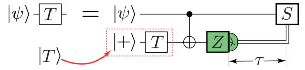
Figure 30: Application of a logical $T$-gate through the injection of a magic state by teleporting. The magic state should be distilled beforehand. Figure taken from [227].

Coming back to the topic of decoding algorithms, note that if one restricts the operation of the QEC to the set of Clifford gates, then due to the fact that the Clifford group is the normalizer of the Pauli group, it is not necessary to know the logical state for applying the circuit [56]. Since Clifford gates map Paulis into Paulis, the only thing that changes is the interpretation of the final measurements after the computation. Therefore, when running such circuits, one can record the syndrome history during the computation and post-process the errors using the recorded syndrome information. In this sense, one can construct a quantum memory without requiring real-time decoding [56]. However, the scenario drastically changes whenever useful computations are taken into account. That is because when injecting the magic state, one must be certain if the $S$-gate after the measurement should be applied or not. Such a decision can only be reliably performed if the syndrome data before the application of said gate is decoded [227]. If the correction of such a Clifford error is ignored, the resulting error might propagate into a much more complicated error that will corrupt the computation [56]. Therefore, in a fault-tolerant quantum computer, the classical processing of the syndrome data, that is, the decoding algorithm; should be fast enough so that syndrome data does not accumulate into an undecodable degree. This accumulation of syndrome data due to the latency of the decoding algorithm is usually referred as the backlog problem [56, 227]. $r_{\mathrm{proc}}$ is defined as the rate at which the decoder processes the syndrome data while $r_{\mathrm{gen}}$ is the rate at which the syndrome data is generated (both quantities in bauds). As discussed by Terhal in [56], if the ratio $r_{\mathrm{gen}}/r_{\mathrm{proc}}=f>1$, then a small initial backlog in the processing of the syndrome data will result in an exponential slow down as a function of the $T$-gate depth of the algorithm. More concretely, Terhal lower bounded the running time of $k$ $T$-depth quantum algorithms as $cf^{k}$ when $f>1$, for some constant $c$ [56, 227]. Thus, the straightforward conclusion is that decoding algorithms must be fast enough to ensure that the injections of the magic states are delayed by only a constant amount of time (instead of an exponentially increasing amount of time).

Appendix B Multiple-round decoding for measurement errors

Throughout this article, surface code decoders have been described as correcting errors arising from data qubit errors, i.e. considering that check measuremnts are noiseless. However, this simplified perspective is overly optimistic because circuit-level noise arising from gate and SPAM errors make syndrome measurement to be noisy too. As mentioned in the main article section on error models and decoding, circuit level noise will lead to incorrect syndromes. If we attempt to decode an erroneous syndrome, the recovered error will likely result in a logical error. Therefore, a new approach is needed to account this type of errors in the code. The common technique consists in performing multiple syndrome extracting rounds. When a check qubit undergoes a change in its measurement value, it implies a non-trivial syndrome element for such measurement round. Subsequently, decoding algorithms can be employed by connecting check qubits within a particular time instance to themselves in the following time, creating a graph containing space and time information of the errors. Recall that not every decoding algorithm requires this multiple-round measurements as, for example, the cellular automaton decoders [124, 186]. These type of decoders are usually known as single-shot decoders [161]. It is important to say that not every QEC family can admit a single-shot decoding algorithm [161].

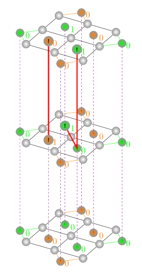
Figure 31: Graphical representation of an error in a space-time surface code.

FIG. 31 illustrates a graphical depiction of three decoding rounds. In this example, three rounds of syndrome extraction have been computed, where the temporal direction progresses upwards. During the initial syndrome extraction, all checks yield a measurement of 0, assuming an absence of errors. This set of measurements serves as the starting point. In the subsequent syndrome extraction, two checks undergo a measurement change: a green $X$-check transitions into 1, as does an orange $Z$-check. These altered check measurements are classified as non-trivial syndrome elements. In the third round, the measurement values of two checks change again, designating them as non-trivial syndrome elements. One of these checks is the orange check from the second decoding round, which reverts back to 0, while the other one is an $X$-check. It is worth noting that although the $X$-check from the second syndrome extraction retains a measurement value of 1, it is not considered a non-trivial syndrome element since its measurement value did not change.

The common approach for considering measurement error noise channels consists in introducing an error probability to the state initialization of the measurement qubit, noisy Haddamard and CNOT gates as described in the error model section and noisy measurement probabilities. Often, this is done by considering all gates within the syndrome measurement circuits from FIG. 3, with probability $p$ [32]. For example, a CNOT is a two gate which has probability $p/15$ a non-trivial two-fold Pauli operator ($I\otimes X,I\otimes Y,\dots,Z\otimes Z$). Often, the noise channel considered for gate errors is the depolarizing channel, but there have also been studies which have considered biased channels so as to reproduce results which may reflect the bias suffered by several experimental qubits.

To implement perfect matching methods like MWPM or UF, the dashed purple lines in FIG. 31 are taken into account. These lines represent edges that connect different time instances separated by one syndrome extraction. The resulting perfect matching will consist of space edges and time edges. Space edges correspond to Pauli errors within the data qubits, while time edges represent faulty measurements that do not require actual error recovery within the code. In FIG. 31, a potential perfect matching is indicated by red lines, which consist of two time edges and one space edge.

An interesting approach to the decoding of surface codes under circuit-level noise and several decoding rounds was given in [87], where they consider the errors that may arise from the stabilizing circuit. When a set of errors is indistinguishable (they trigger the same measurement qubits), they are considered equal events under the combination of their probabilities. With these considerations in mind, a Tanner graph can be developed considering all syndrome measurement rounds. A graphic illustration is provided in FIG. 32, in the top figure one can see a planar representation of the stabilizing circuit of a distance-3 surface code. Note that by following the CNOT order given by the violet numbers one can compute all the CNOT gates of the surface code stabilizing circuit with only 4 steps avoiding at all time that one qubit experiences two CNOT gates at the same time. The measurement qubits, which are also defined as detectors in the literature, are denoted with $D_{i}$ labels. After several stabilizing measurements we can describe the overall syndrome through the change in parities of the detectors as shown in FIG. 31, i.e. the syndrome element $D_{i}^{t}$ will be 1 if the detector $D_{i}$ has changed its measurement outcome between the measurement time instances $t-1$ and $t$. Within the top figure, one of the CNOT gates are written in red, in the bottom figure, a Tanner graph relates the possible Pauli errors which may occur in the noisy CNOT gate with the detector events they would trigger. Consider the case of a $ZX$ error, which is highlighted in orange lines. The $X$ operator on the data qubit which is applied on the circuit time step $3$ will propagate to $D_{3}$ in the following circuit time step following the logic of FIG. 3 and producing a non-trivial $D_{3}^{t}$ due to the parity change in its measurement. In the following round of measurements the $X$ error from the data qubit will propagate to $D_{2}$ changing its parity and producing a non-trivial $D_{2}^{t+1}$. On the other hand, the $Z$ error correspondent to the detector will produce a measurement error, changing its parity and resulting in a non-trivial $D_{6}^{t}$. After another stabilizing round, the parity of the detector changes again since there is no measurement error and so it returns to the previous state, making $D_{6}^{t+1}$ also be non-trivial. FIG. 32 only contains the Tanner graph correspondent to a CNOT error, in order to consider the entire surface code circuit level noise, one should consider all CNOT error Tanner graphs omitting operators which trigger the same set of operators, doing so allows to compute BP, which aids other decoding methods such as MWPM or UF in their task of decoding a syndrome [87]. This method has also been considered for the BPOSD method in [238], where the authors decode a low connection QLDPC code by considering the gate and idling Pauli errors.

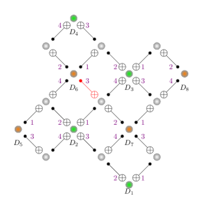
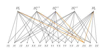
Figure 32: In the top, a distance-3 surface code with the CNOT gates from the stabilizing circuit shown. The violet numbers indicate the order at which the CNOT gates are applied within the circuit of every measurement qubit, which themselves are labelled as $D_{i}$. Graphical representation of the circuit-level Tanner graph from a single CNOT, which is denoted in red. The figure is inspired from [87].

Usually, it is considered that a distance-$d$ surface code requires $\mathcal{O}(d)$ syndrome extraction rounds per decoding round [87, 107, 83] in order to preserve the distance property. Considering several syndrome extractions further complicates the decoding process, since it significantly increases the number of nodes within decoding graphs and the connectivity of the graph. Specifically, a surface code of arbitrary distance-$d$, which has $d^{2}-1$ checks, results to have $d(d^{2}-1)$ checks. Moreover, even by considering multiple decoding rounds for dealing with faulty measurements, the threshold of the codes decrease dramatically due to such effect caused by circuit-level noise when compared to just data qubit noise [32, 87, 107].

In conclusion, measurement errors pose a significant challenge to the successful implementation of the surface code. The accurate extraction of syndromes is crucial for effective error correction. Faulty-measurements lead to lower code thresholds, implying that the hardware requirements for error correction are more stringent. Therefore, dealing with circuit-level noise and noisy measurements is critical to reach the fault-tolerant quantum computing paradigm.

Appendix C QECC numerical simulations

Monte Carlo computer simulations of the $d\times d$ rotated planar codes with $d\in\{3,5,7,9,11\}$ have been performed with the objective of obtaining the performance curves and thresholds of the code when decoded with MWPM, UF, BPOSD and TN decoders.

Each round of the numerical simulation is performed by generating an $N$-qubit Pauli operator, calculating its associated syndrome, and finally running the decoding algorithm using the associated syndrome as its input (note that for the simulations performed in this paper, no SPAM or gate errors are considered). Once the error is estimated by the decoder, it is used to determine if a logical error has occurred on the codestate by using the channel error [128]. The operational figure of merit we use to evaluate the performance of these quantum error correction schemes is the Logical Error Rate ($P_{L}$), i.e. the probability that a logical error has occurred after the recovery operation.

Regarding the software implementations of the decoders used to obtain the simulations in Section 5 have been: QECSIM for the MWPM and tensor network decoder [180], the BPOSD implementation of Joschka Roffe for the BPOSD decoder [218] and an implementation coded by ourselves for the UF decoder by Delfosse and Nickerson [109].

For the numerical Monte Carlo methods employed to estimate the $P_{L}$ of the rotated planar codes, we have applied the following rule of thumb to select the number of simulation runs, $N_{\mathrm{runs}}$ [239], as

$$N_{\mathrm{runs}}=\frac{100}{P_{L}}.$$ (23)

As explained in [239], under the assumption that the observed error events are independent, this results in a $95\%$ confidence interval of about $(0.8\hat{P_{L}},1.25\hat{P_{L}})$, where $\hat{P_{L}}$ refers to the empirically estimated value for the logical error rate.

References

- [1] Richard P Feynman. “Simulating physics with computers”. International journal of theoretical physics 21, 467–488 (1982).
- [2] John Preskill. “Quantum computing and the entanglement frontier” (2012). arXiv:1203.5813.
- [3] P.W. Shor. “Algorithms for quantum computation: discrete logarithms and factoring”. In Proceedings 35th Annual Symposium on Foundations of Computer Science. Pages 124–134. (1994).
- [4] Ashley Montanaro. “Quantum algorithms: an overview”. npj Quantum Information 2, 15023 (2016).
- [5] C. H. Bennett and G. Brassard. “Quantum cryptography: Public key distribution and coin tossing”. In Proceedings of IEEE International Conference on Computers, Systems, and Signal Processing. Page 175. India (1984).
- [6] Artur K. Ekert. “Quantum cryptography based on bell’s theorem”. Phys. Rev. Lett. 67, 661–663 (1991).
- [7] Kishor Bharti, Alba Cervera-Lierta, Thi Ha Kyaw, Tobias Haug, Sumner Alperin-Lea, Abhinav Anand, Matthias Degroote, Hermanni Heimonen, Jakob S. Kottmann, Tim Menke, Wai-Keong Mok, Sukin Sim, et al. “Noisy intermediate-scale quantum algorithms”. Rev. Mod. Phys. 94, 015004 (2022).
- [8] Nathan Wiebe, Daniel Braun, and Seth Lloyd. “Quantum algorithm for data fitting”. Phys. Rev. Lett. 109, 050505 (2012).
- [9] Jacob Biamonte, Peter Wittek, Nicola Pancotti, Patrick Rebentrost, Nathan Wiebe, and Seth Lloyd. “Quantum machine learning”. Nature 549, 195–202 (2017).
- [10] Carlos Outeiral, Martin Strahm, Jiye Shi, Garrett M. Morris, Simon C. Benjamin, and Charlotte M. Deane. “The prospects of quantum computing in computational molecular biology”. WIREs Computational Molecular Science 11, e1481 (2021).
- [11] Pauline J. Ollitrault, Alexander Miessen, and Ivano Tavernelli. “Molecular quantum dynamics: A quantum computing perspective”. Accounts of Chemical Research 54, 4229–4238 (2021).
- [12] Mohammad Hassan Khatami, Udson C Mendes, Nathan Wiebe, and Philip M Kim. “Gate-based quantum computing for protein design”. PLoS Comput. Biol. 19, e1011033 (2023).
- [13] Daniel Jafferis, Alexander Zlokapa, Joseph D. Lykken, David K. Kolchmeyer, Samantha I. Davis, Nikolai Lauk, Hartmut Neven, and Maria Spiropulu. “Traversable wormhole dynamics on a quantum processor”. Nature 612, 51–55 (2022).
- [14] Steven D. Bass and Erez Zohar. “Quantum technologies in particle physics”. Philosophical Transactions of the Royal Society A: Mathematical, Physical and Engineering Sciences 380, 20210072 (2022).
- [15] Frank Arute, Kunal Arya, Ryan Babbush, Dave Bacon, Joseph C. Bardin, Rami Barends, Rupak Biswas, Sergio Boixo, Fernando G. S. L. Brandao, David A. Buell, et al. “Quantum supremacy using a programmable superconducting processor”. Nature 574, 505–510 (2019).
- [16] Han-Sen Zhong, Hui Wang, Yu-Hao Deng, Ming-Cheng Chen, Li-Chao Peng, Yi-Han Luo, Jian Qin, Dian Wu, Xing Ding, Yi Hu, Peng Hu, et al. “Quantum computational advantage using photons”. Science 370, 1460–1463 (2020).
- [17] Yulin Wu, Wan-Su Bao, Sirui Cao, Fusheng Chen, Ming-Cheng Chen, Xiawei Chen, Tung-Hsun Chung, Hui Deng, Yajie Du, Daojin Fan, Ming Gong, et al. “Strong quantum computational advantage using a superconducting quantum processor”. Phys. Rev. Lett. 127, 180501 (2021).
- [18] Hsin-Yuan Huang, Michael Broughton, Jordan Cotler, Sitan Chen, Jerry Li, Masoud Mohseni, Hartmut Neven, Ryan Babbush, Richard Kueng, John Preskill, and Jarrod R. McClean. “Quantum advantage in learning from experiments”. Science 376, 1182–1186 (2022).
- [19] Lars S. Madsen, Fabian Laudenbach, Mohsen Falamarzi. Askarani, Fabien Rortais, Trevor Vincent, Jacob F. F. Bulmer, Filippo M. Miatto, Leonhard Neuhaus, Lukas G. Helt, Matthew J. Collins, Adriana E. Lita, et al. “Quantum computational advantage with a programmable photonic processor”. Nature 606, 75–81 (2022).
- [20] Michael A. Nielsen and Isaac L. Chuang. “Quantum computation and quantum information: 10th anniversary edition”. Cambridge University Press. USA (2011). 10th edition.
- [21] Yulin Chi, Jieshan Huang, Zhanchuan Zhang, Jun Mao, Zinan Zhou, Xiaojiong Chen, Chonghao Zhai, Jueming Bao, Tianxiang Dai, Huihong Yuan, Ming Zhang, et al. “A programmable qudit-based quantum processor”. Nature Communications 13, 1166 (2022).
- [22] Robert Raussendorf and Hans J. Briegel. “A one-way quantum computer”. Phys. Rev. Lett. 86, 5188–5191 (2001).
- [23] H. J. Briegel, D. E. Browne, W. Dür, R. Raussendorf, and M. Van den Nest. “Measurement-based quantum computation”. Nature Physics 5, 19–26 (2009).
- [24] Anjan K. Chandra, Arnab Das, and Bikas K. Chakrabarti. “Quantum quenching, annealing and computation”. Springer-Verlag Berlin. DE (2010). 1 edition.
- [25] Atharv Joshi, Kyungjoo Noh, and Yvonne Y Gao. “Quantum information processing with bosonic qubits in circuit qed”. Quantum Science and Technology 6, 033001 (2021).
- [26] He-Liang Huang, Dachao Wu, Daojin Fan, and Xiaobo Zhu. “Superconducting quantum computing: a review”. Science China Information Sciences 63, 180501 (2020).
- [27] H. Häffner, C.F. Roos, and R. Blatt. “Quantum computing with trapped ions”. Physics Reports 469, 155–203 (2008).
- [28] Sergei Slussarenko and Geoff J. Pryde. “Photonic quantum information processing: A concise review”. Applied Physics Reviews6 (2019).
- [29] Peter W. Shor. “Scheme for reducing decoherence in quantum computer memory”. Phys. Rev. A 52, R2493–R2496 (1995).
- [30] Josu Etxezarreta Martinez, Patricio Fuentes, Pedro M. Crespo, and J. Garcia-Frias. “Approximating decoherence processes for the design and simulation of quantum error correction codes on classical computers”. IEEE Access 8, 172623–172643 (2020).
- [31] J. M. Chow, J. M. Gambetta, L. Tornberg, Jens Koch, Lev S. Bishop, A. A. Houck, B. R. Johnson, L. Frunzio, S. M. Girvin, and R. J. Schoelkopf. “Randomized benchmarking and process tomography for gate errors in a solid-state qubit”. Phys. Rev. Lett. 102, 090502 (2009).
- [32] Austin G. Fowler, Matteo Mariantoni, John M. Martinis, and Andrew N. Cleland. “Surface codes: Towards practical large-scale quantum computation”. Phys. Rev. A 86, 032324 (2012).
- [33] John Preskill. “Quantum Computing in the NISQ era and beyond”. Quantum 2, 79 (2018).
- [34] Jonathan J. Burnett, Andreas Bengtsson, Marco Scigliuzzo, David Niepce, Marina Kudra, Per Delsing, and Jonas Bylander. “Decoherence benchmarking of superconducting qubits”. npj Quantum Information 5, 54 (2019).
- [35] Josu Etxezarreta Martinez, Patricio Fuentes, Pedro Crespo, and Javier Garcia-Frias. “Time-varying quantum channel models for superconducting qubits”. npj Quantum Information 7, 115 (2021).
- [36] I. S. Reed and G. Solomon. “Polynomial codes over certain finite fields”. Journal of the Society for Industrial and Applied Mathematics 8, 300–304 (1960).
- [37] R. Gallager. “Low-density parity-check codes”. IRE Transactions on Information Theory 8, 21–28 (1962).
- [38] C. Berrou, A. Glavieux, and P. Thitimajshima. “Near shannon limit error-correcting coding and decoding: Turbo-codes. 1”. In Proceedings of ICC ’93 - IEEE International Conference on Communications. Volume 2, pages 1064–1070 vol.2. (1993).
- [39] Daniel Gottesman. “Stabilizer codes and quantum error correction”. Phd thesis. California Institute of Technology. Pasadena, CA (1997).
- [40] A.Yu. Kitaev. “Fault-tolerant quantum computation by anyons”. Annals of Physics 303, 2–30 (2003).
- [41] J. Pablo Bonilla Ataides, David K. Tuckett, Stephen D. Bartlett, Steven T. Flammia, and Benjamin J. Brown. “The xzzx surface code”. Nature Communications 12, 2172 (2021).
- [42] David K. Tuckett, Stephen D. Bartlett, and Steven T. Flammia. “Ultrahigh error threshold for surface codes with biased noise”. Phys. Rev. Lett. 120, 050505 (2018).
- [43] Christopher Chamberland, Guanyu Zhu, Theodore J. Yoder, Jared B. Hertzberg, and Andrew W. Cross. “Topological and subsystem codes on low-degree graphs with flag qubits”. Phys. Rev. X 10, 011022 (2020).
- [44] H. Bombin and M. A. Martin-Delgado. “Topological quantum distillation”. Phys. Rev. Lett. 97, 180501 (2006).
- [45] D.J.C. MacKay, G. Mitchison, and P.L. McFadden. “Sparse-graph codes for quantum error correction”. IEEE Transactions on Information Theory 50, 2315–2330 (2004).
- [46] Pavel Panteleev and Gleb Kalachev. “Degenerate Quantum LDPC Codes With Good Finite Length Performance”. Quantum 5, 585 (2021).
- [47] Pavel Panteleev and Gleb Kalachev. “Quantum ldpc codes with almost linear minimum distance”. IEEE Transactions on Information Theory 68, 213–229 (2022).
- [48] Pavel Panteleev and Gleb Kalachev. “Asymptotically Good Quantum and Locally Testable Classical LDPC Codes” (2021). arXiv:2111.03654.
- [49] Nikolas P. Breuckmann and Jens Niklas Eberhardt. “Quantum low-density parity-check codes”. PRX Quantum 2, 040101 (2021).
- [50] Patricio Fuentes, Josu Etxezarreta Martinez, Pedro M. Crespo, and Javier Garcia-Frias. “Approach for the construction of non-calderbank-steane-shor low-density-generator-matrix–based quantum codes”. Phys. Rev. A 102, 012423 (2020).
- [51] David Poulin, Jean-Pierre Tillich, and Harold Ollivier. “Quantum serial turbo codes”. IEEE Transactions on Information Theory 55, 2776–2798 (2009).
- [52] Mark M. Wilde, Min-Hsiu Hsieh, and Zunaira Babar. “Entanglement-assisted quantum turbo codes”. IEEE Transactions on Information Theory 60, 1203–1222 (2014).
- [53] Josu Etxezarreta Martinez, Pedro M. Crespo, and Javier Garcia-Frías. “Depolarizing channel mismatch and estimation protocols for quantum turbo codes”. Entropy 21, 1133 (2019).
- [54] Patricio Fuentes, Josu Etxezarreta Martinez, Pedro M. Crespo, and Javier Garcia-Frías. “Degeneracy and its impact on the decoding of sparse quantum codes”. IEEE Access 9, 89093–89119 (2021).
- [55] Pavithran Iyer and David Poulin. “Hardness of decoding quantum stabilizer codes”. IEEE Transactions on Information Theory 61, 5209–5223 (2015).
- [56] Barbara M. Terhal. “Quantum error correction for quantum memories”. Rev. Mod. Phys. 87, 307–346 (2015).
- [57] Oscar Higgott and Craig Gidney. “Sparse Blossom: correcting a million errors per core second with minimum-weight matching” (2023). arXiv:2303.15933.
- [58] Sergey Bravyi, Matthias Englbrecht, Robert König, and Nolan Peard. “Correcting coherent errors with surface codes”. npj Quantum Information 4, 55 (2018).
- [59] Eric Dennis, Alexei Kitaev, Andrew Landahl, and John Preskill. “Topological quantum memory”. Journal of Mathematical Physics 43, 4452–4505 (2002).
- [60] Robert Raussendorf and Jim Harrington. “Fault-tolerant quantum computation with high threshold in two dimensions”. Phys. Rev. Lett. 98, 190504 (2007).
- [61] Austin G. Fowler, Ashley M. Stephens, and Peter Groszkowski. “High-threshold universal quantum computation on the surface code”. Phys. Rev. A 80, 052312 (2009).
- [62] H. Bombin and M. A. Martin-Delgado. “Optimal resources for topological two-dimensional stabilizer codes: Comparative study”. Phys. Rev. A 76, 012305 (2007).
- [63] Sebastian Krinner, Nathan Lacroix, Ants Remm, Agustin Di Paolo, Elie Genois, Catherine Leroux, Christoph Hellings, Stefania Lazar, Francois Swiadek, Johannes Herrmann, Graham J. Norris, et al. “Realizing repeated quantum error correction in a distance-three surface code”. Nature 605, 669–674 (2022).
- [64] Rajeev Acharya, Igor Aleiner, Richard Allen, Trond I. Andersen, Markus Ansmann, Frank Arute, Kunal Arya, Abraham Asfaw, Juan Atalaya, Ryan Babbush, Dave Bacon, et al. “Suppressing quantum errors by scaling a surface code logical qubit”. Nature 614, 676–681 (2023).
- [65] Benjamin Schumacher. “Quantum coding”. Phys. Rev. A 51, 2738–2747 (1995).
- [66] A. Einstein, B. Podolsky, and N. Rosen. “Can quantum-mechanical description of physical reality be considered complete?”. Phys. Rev. 47, 777–780 (1935).
- [67] David P. DiVincenzo, Peter W. Shor, and John A. Smolin. “Quantum-channel capacity of very noisy channels”. Phys. Rev. A 57, 830–839 (1998).
- [68] Graeme Smith and Jon Yard. “Quantum communication with zero-capacity channels”. Science 321, 1812–1815 (2008).
- [69] M. B. Hastings. “Superadditivity of communication capacity using entangled inputs”. Nature Physics 5, 255–257 (2009).
- [70] Josu Etxezarreta Martinez, Antonio deMarti iOlius, and Pedro M. Crespo. “Superadditivity effects of quantum capacity decrease with the dimension for qudit depolarizing channels”. Phys. Rev. A 108, 032602 (2023).
- [71] Todd A. Brun, Igor Devetak, and Min-Hsiu Hsieh. “Catalytic quantum error correction”. IEEE Transactions on Information Theory 60, 3073–3089 (2014).
- [72] Misty A. Wahl, Andrea Mari, Nathan Shammah, William J. Zeng, and Gokul Subramanian Ravi. “Zero noise extrapolation on logical qubits by scaling the error correction code distance” (2023). arXiv:2304.14985.
- [73] Abhinav Kandala, Kristan Temme, Antonio D. Córcoles, Antonio Mezzacapo, Jerry M. Chow, and Jay M. Gambetta. “Error mitigation extends the computational reach of a noisy quantum processor”. Nature 567, 491–495 (2019).
- [74] Ewout van den Berg, Zlatko K. Minev, Abhinav Kandala, and Kristan Temme. “Probabilistic error cancellation with sparse pauli–lindblad models on noisy quantum processors”. Nature Physics (2023).
- [75] Youngseok Kim, Andrew Eddins, Sajant Anand, Ken Xuan Wei, Ewout van den Berg, Sami Rosenblatt, Hasan Nayfeh, Yantao Wu, Michael Zaletel, Kristan Temme, and Abhinav Kandala. “Evidence for the utility of quantum computing before fault tolerance”. Nature 618, 500–505 (2023).
- [76] Zhenyu Cai, Ryan Babbush, Simon C. Benjamin, Suguru Endo, William J. Huggins, Ying Li, Jarrod R. McClean, and Thomas E. O’Brien. “Quantum Error Mitigation” (2022). arXiv:2210.00921.
- [77] Todd Brun, Igor Devetak, and Min-Hsiu Hsieh. “Correcting quantum errors with entanglement”. Science 314, 436–439 (2006).
- [78] Josu Etxezarreta Martinez. “Decoherence and quantum error correction for quantum computing and communications”. Phd thesis. Tecnun - Universidad de Navarra. Donostia, Spain (2022).
- [79] Emanuel Knill and Raymond Laflamme. “Theory of quantum error-correcting codes”. Phys. Rev. A 55, 900–911 (1997).
- [80] Min-Hsiu Hsieh and Fran çois Le Gall. “Np-hardness of decoding quantum error-correction codes”. Phys. Rev. A 83, 052331 (2011).
- [81] Kao-Yueh Kuo and Chung-Chin Lu. “On the hardness of decoding quantum stabilizer codes under the depolarizing channel”. In 2012 International Symposium on Information Theory and its Applications. Pages 208–211. (2012).
- [82] Kao-Yueh Kuo and Chung-Chin Lu. “On the hardnesses of several quantum decoding problems”. Quantum Information Processing 19, 123 (2020).
- [83] Dominic Horsman, Austin G Fowler, Simon Devitt, and Rodney Van Meter. “Surface code quantum computing by lattice surgery”. New Journal of Physics 14, 123011 (2012).
- [84] Sergey B. Bravyi and Alexei Yu. Kitaev. “Quantum codes on a lattice with boundary” (1998). arXiv:quant-ph/9811052.
- [85] A. R. Calderbank and Peter W. Shor. “Good quantum error-correcting codes exist”. Phys. Rev. A 54, 1098–1105 (1996).
- [86] Andrew Steane. “Multiple-particle interference and quantum error correction”. Proceedings: Mathematical, Physical and Engineering Sciences 452, 2551–2577 (1996).
- [87] Oscar Higgott, Thomas C. Bohdanowicz, Aleksander Kubica, Steven T. Flammia, and Earl T. Campbell. “Improved decoding of circuit noise and fragile boundaries of tailored surface codes”. Phys. Rev. X 13, 031007 (2023).
- [88] Antonio deMarti iOlius, Josu Etxezarreta Martinez, Patricio Fuentes, and Pedro M. Crespo. “Performance enhancement of surface codes via recursive minimum-weight perfect-match decoding”. Phys. Rev. A 108, 022401 (2023).
- [89] Yuuki Tokunaga and Keisuke Fujii. “Thresholds of surface codes on the general lattice structures suffering biased error and loss”. AIP Conference Proceedings 1633, 198–200 (2014).
- [90] Dorit Aharonov and Michael Ben-Or. “Fault-tolerant quantum computation with constant error rate”. SIAM Journal on Computing 38, 1207–1282 (2008).
- [91] Emanuel Knill, Raymond Laflamme, and Wojciech H. Zurek. “Resilient quantum computation”. Science 279, 342–345 (1998).
- [92] Steffen Schlör. “Intrinsic decoherence in superconducting quantum circuits”. Phd thesis. Karlsruher Institut für Technologie. Karlsruhe, Germany (2019).
- [93] Angel Rivas and Susana F. Huelga. “Open quantum systems - an introduction”. Springer Berlin, Heidelberg. DE (2011). 1 edition.
- [94] Q. A. Turchette, C. J. Myatt, B. E. King, C. A. Sackett, D. Kielpinski, W. M. Itano, C. Monroe, and D. J. Wineland. “Decoherence and decay of motional quantum states of a trapped atom coupled to engineered reservoirs”. Phys. Rev. A 62, 053807 (2000).
- [95] Vittorio Gorini, Andrzej Kossakowski, and E. C. G. Sudarshan. “Completely positive dynamical semigroups of N-level systems”. Journal of Mathematical Physics 17, 821–825 (1976).
- [96] G. Lindblad. “On the generators of quantum dynamical semigroups”. Communications in Mathematical Physics 48, 119–130 (1976).
- [97] Man-Duen Choi. “Completely positive linear maps on complex matrices”. Linear Algebra and its Applications 10, 285–290 (1975).
- [98] Sumeet Khatri, Kunal Sharma, and Mark M. Wilde. “Information-theoretic aspects of the generalized amplitude-damping channel”. Phys. Rev. A 102, 012401 (2020).
- [99] L. Lami and V. Giovannetti. “Entanglement–breaking indices”. Journal of Mathematical Physics56 (2015).
- [100] Pradeep Kiran Sarvepalli, Andreas Klappenecker, and Martin Rötteler. “Asymmetric quantum codes: constructions, bounds and performance”. Proceedings of the Royal Society A: Mathematical, Physical and Engineering Sciences 465, 1645–1672 (2009).
- [101] Joseph Emerson, Marcus Silva, Osama Moussa, Colm Ryan, Martin Laforest, Jonathan Baugh, David G. Cory, and Raymond Laflamme. “Symmetrized characterization of noisy quantum processes”. Science 317, 1893–1896 (2007).
- [102] M. Silva, E. Magesan, D. W. Kribs, and J. Emerson. “Scalable protocol for identification of correctable codes”. Phys. Rev. A 78, 012347 (2008).
- [103] D Gottesman. “The heisenberg representation of quantum computers”. Proceedings of the XXII International Colloquium on Group Theoretical Methods in Physics (1998).
- [104] Antonio deMarti iOlius, Josu Etxezarreta Martinez, Patricio Fuentes, Pedro M. Crespo, and Javier Garcia-Frias. “Performance of surface codes in realistic quantum hardware”. Phys. Rev. A 106, 062428 (2022).
- [105] Robin Harper and Steven T. Flammia. “Learning correlated noise in a 39-qubit quantum processor” (2023). arXiv:2303.00780.
- [106] Konstantin Tiurev, Peter-Jan H. S. Derks, Joschka Roffe, Jens Eisert, and Jan-Michael Reiner. “Correcting non-independent and non-identically distributed errors with surface codes” (2022). arXiv:2208.02191.
- [107] Christopher Chamberland and Earl T. Campbell. “Universal quantum computing with twist-free and temporally encoded lattice surgery”. PRX Quantum 3, 010331 (2022).
- [108] Stefano Mangini, Lorenzo Maccone, and Chiara Macchiavello. “Qubit noise deconvolution”. EPJ Quantum Technology 9, 29 (2022).
- [109] Nicolas Delfosse and Naomi H. Nickerson. “Almost-linear time decoding algorithm for topological codes”. Quantum 5, 595 (2021).
- [110] M. Grassl, Th. Beth, and T. Pellizzari. “Codes for the quantum erasure channel”. Phys. Rev. A 56, 33–38 (1997).
- [111] Francesco Battistel. “Mitigating leakage and noise in superconducting quantum computing”. Phd thesis. TU Delft. Delft, Netherlands (2022).
- [112] Roman Stricker, Davide Vodola, Alexander Erhard, Lukas Postler, Michael Meth, Martin Ringbauer, Philipp Schindler, Thomas Monz, Markus Müller, and Rainer Blatt. “Experimental deterministic correction of qubit loss”. Nature 585, 207–210 (2020).
- [113] Joydip Ghosh, Austin G. Fowler, John M. Martinis, and Michael R. Geller. “Understanding the effects of leakage in superconducting quantum-error-detection circuits”. Phys. Rev. A 88, 062329 (2013).
- [114] Niels Bohr. “On the constitution of atoms and molecules”. Pages 13–33. Springer International Publishing. Cham (1913).
- [115] Th. Sauter, W. Neuhauser, R. Blatt, and P. E. Toschek. “Observation of quantum jumps”. Phys. Rev. Lett. 57, 1696–1698 (1986).
- [116] Ayumu Nakayama and Manabu Hagiwara. “Single quantum deletion error-correcting codes”. In 2020 International Symposium on Information Theory and Its Applications (ISITA). Pages 329–333. (2020).
- [117] Jack Edmonds. “Paths, trees, and flowers”. Canadian Journal of Mathematics 17, 449–467 (1965).
- [118] Yue Wu. “Fusion blossom” (2022).
- [119] Yue Wu and Lin Zhong. “Fusion Blossom: Fast MWPM Decoders for QEC” (2023). arXiv:2305.08307.
- [120] Oscar Higgott. “Pymatching: A python package for decoding quantum codes with minimum-weight perfect matching”. ACM Transactions on Quantum Computing3 (2022).
- [121] Sergey Bravyi, Martin Suchara, and Alexander Vargo. “Efficient algorithms for maximum likelihood decoding in the surface code”. Phys. Rev. A 90, 032326 (2014).
- [122] Joschka Roffe, David R. White, Simon Burton, and Earl Campbell. “Decoding across the quantum low-density parity-check code landscape”. Phys. Rev. Res. 2, 043423 (2020).
- [123] Guillaume Duclos-Cianci and David Poulin. “Fast decoders for topological quantum codes”. Phys. Rev. Lett. 104, 050504 (2010).
- [124] Michael Herold, Earl T. Campbell, Jens Eisert, and Michael J. Kastoryano. “Cellular-automaton decoders for topological quantum memories”. npj Quantum Information 1, 15010 (2015).
- [125] Savvas Varsamopoulos, Ben Criger, and Koen Bertels. “Decoding small surface codes with feedforward neural networks”. Quantum Science and Technology 3, 015004 (2017).
- [126] Lucas Berent, Lukas Burgholzer, Peter-Jan H. S. Derks, Jens Eisert, and Robert Wille. “Decoding quantum color codes with MaxSAT” (2023). arXiv:2303.14237.
- [127] Austin G. Fowler. “Minimum weight perfect matching of fault-tolerant topological quantum error correction in average o(1) parallel time”. Quantum Info. Comput. 15, 145–158 (2015).
- [128] Patricio Fuentes, Josu Etxezarreta Martinez, Pedro M. Crespo, and Javier Garcia-Frías. “On the logical error rate of sparse quantum codes”. IEEE Transactions on Quantum Engineering 3, 1–12 (2022).
- [129] Sergey Bravyi and Matthew B. Hastings. “Homological product codes”. In Proceedings of the Forty-Sixth Annual ACM Symposium on Theory of Computing. Page 273–282. STOC ’14New York, NY, USA (2014). Association for Computing Machinery.
- [130] Yue Wu, Namitha Liyanage, and Lin Zhong. “An interpretation of Union-Find Decoder on Weighted Graphs” (2022). arXiv:2211.03288.
- [131] Jonghyun Lee, Jooyoun Park, and Jun Heo. “Rectangular surface code under biased noise”. Quantum Information Processing 20, 231 (2021).
- [132] David K. Tuckett, Stephen D. Bartlett, Steven T. Flammia, and Benjamin J. Brown. “Fault-tolerant thresholds for the surface code in excess of under biased noise”. Phys. Rev. Lett. 124, 130501 (2020).
- [133] Josu Etxezarreta Martinez, Patricio Fuentes, Antonio deMarti iOlius, Javier Garcia-Frias, Javier Rodríguez Fonollosa, and Pedro M. Crespo. “Multiqubit time-varying quantum channels for nisq-era superconducting quantum processors”. Phys. Rev. Res. 5, 033055 (2023).
- [134] Nicolas Delfosse and Jean-Pierre Tillich. “A decoding algorithm for css codes using the x/z correlations”. In 2014 IEEE International Symposium on Information Theory. Pages 1071–1075. (2014).
- [135] Austin G. Fowler. “Optimal complexity correction of correlated errors in the surface code” (2013). arXiv:1310.0863.
- [136] Craig Gidney. “Stim: a fast stabilizer circuit simulator”. Quantum 5, 497 (2021). arXiv:2103.02202.
- [137] Nicolas Delfosse and Gilles Zémor. “Linear-time maximum likelihood decoding of surface codes over the quantum erasure channel”. Phys. Rev. Res. 2, 033042 (2020).
- [138] Robert Endre Tarjan. “Efficiency of a good but not linear set union algorithm”. J. ACM 22, 215–225 (1975).
- [139] Shilin Huang, Michael Newman, and Kenneth R. Brown. “Fault-tolerant weighted union-find decoding on the toric code”. Phys. Rev. A 102, 012419 (2020).
- [140] Nicolas Delfosse, Vivien Londe, and Michael E. Beverland. “Toward a union-find decoder for quantum ldpc codes”. IEEE Transactions on Information Theory 68, 3187–3199 (2022).
- [141] Judea Pearl. “Probabilistic reasoning in intelligent systems”. Morgan Kaufmann. CA, USA (1998). 1 edition.
- [142] F.R. Kschischang, B.J. Frey, and H.-A. Loeliger. “Factor graphs and the sum-product algorithm”. IEEE Transactions on Information Theory 47, 498–519 (2001).
- [143] Niclas Wiberg. “Codes and decoding on general graphs”. Phd thesis. Linköping University,. Linköping , Sweden (1996).
- [144] David Poulin and Yeojin Chung. “On the iterative decoding of sparse quantum codes”. Quantum Info. Comput. 8, 987–1000 (2008).
- [145] Sae-Young Chung, G.D. Forney, T.J. Richardson, and R. Urbanke. “On the design of low-density parity-check codes within 0.0045 db of the shannon limit”. IEEE Communications Letters 5, 58–60 (2001).
- [146] Matthew B. Hastings, Jeongwan Haah, and Ryan O’Donnell. “Fiber Bundle Codes: Breaking the Barrier for Quantum LDPC Codes” (2020). arXiv:2009.03921.
- [147] Nikolas P. Breuckmann and Jens N. Eberhardt. “Balanced product quantum codes”. IEEE Transactions on Information Theory 67, 6653–6674 (2021).
- [148] A. Leverrier and G. Zemor. “Quantum tanner codes”. In 2022 IEEE 63rd Annual Symposium on Foundations of Computer Science (FOCS). Pages 872–883. Los Alamitos, CA, USA (2022). IEEE Computer Society.
- [149] Graeme Smith and John A. Smolin. “Degenerate quantum codes for pauli channels”. Phys. Rev. Lett. 98, 030501 (2007).
- [150] Nithin Raveendran and Bane Vasić. “Trapping Sets of Quantum LDPC Codes”. Quantum 5, 562 (2021).
- [151] Nithin Raveendran. “Trapping sets of iterative decoders for quantum and classical low-density parity check codes”. Phd thesis. The University of Arizona. Arizona, USA (2021).
- [152] M.P.C. Fossorier and Shu Lin. “Soft-decision decoding of linear block codes based on ordered statistics”. IEEE Transactions on Information Theory 41, 1379–1396 (1995).
- [153] M.P.C. Fossorier. “Iterative reliability-based decoding of low-density parity check codes”. IEEE Journal on Selected Areas in Communications 19, 908–917 (2001).
- [154] Joschka Roffe, Lawrence Z. Cohen, Armanda O. Quintavalle, Daryus Chandra, and Earl T. Campbell. “Bias-tailored quantum LDPC codes”. Quantum 7, 1005 (2023).
- [155] Gene H. Golub and Charles F. Van Loan. “Matrix computations”. John Hopkins University Press. EN (2013). 4 edition.
- [156] Javier Valls, Francisco Garcia-Herrero, Nithin Raveendran, and Bane Vasić. “Syndrome-based min-sum vs osd-0 decoders: Fpga implementation and analysis for quantum ldpc codes”. IEEE Access 9, 138734–138743 (2021).
- [157] Julien Du Crest, Mehdi Mhalla, and Valentin Savin. “Stabilizer inactivation for message-passing decoding of quantum ldpc codes”. In 2022 IEEE Information Theory Workshop (ITW). Pages 488–493. (2022).
- [158] Ben Criger and Imran Ashraf. “Multi-path Summation for Decoding 2D Topological Codes”. Quantum 2, 102 (2018).
- [159] Nithin Raveendran, Narayanan Rengaswamy, Asit Kumar Pradhan, and Bane Vasić. “Soft syndrome decoding of quantum ldpc codes for joint correction of data and syndrome errors”. In 2022 IEEE International Conference on Quantum Computing and Engineering (QCE). Pages 275–281. (2022).
- [160] Christopher A. Pattison, Michael E. Beverland, Marcus P. da Silva, and Nicolas Delfosse. “Improved quantum error correction using soft information” (2021). arXiv:2107.13589.
- [161] Oscar Higgott and Nikolas P. Breuckmann. “Improved single-shot decoding of higher-dimensional hypergraph-product codes”. PRX Quantum 4, 020332 (2023).
- [162] Héctor Bombín. “Single-shot fault-tolerant quantum error correction”. Phys. Rev. X 5, 031043 (2015).
- [163] Nikolas P. Breuckmann and Vivien Londe. “Single-shot decoding of linear rate ldpc quantum codes with high performance”. IEEE Transactions on Information Theory 68, 272–286 (2022).
- [164] Shouzhen Gu, Eugene Tang, Libor Caha, Shin Ho Choe, Zhiyang He, and Aleksander Kubica. “Single-shot decoding of good quantum LDPC codes” (2023). arXiv:2306.12470.
- [165] Omar Fawzi, Antoine Grospellier, and Anthony Leverrier. “Constant overhead quantum fault tolerance with quantum expander codes”. Commun. ACM 64, 106–114 (2020).
- [166] R. Orús. “A practical introduction to tensor networks: Matrix product states and projected entangled pair states”. Annals of Physics 349, 117–158 (2014).
- [167] Andrew J. Ferris and David Poulin. “Tensor networks and quantum error correction”. Phys. Rev. Lett. 113, 030501 (2014).
- [168] G. Evenbly and G. Vidal. “Class of highly entangled many-body states that can be efficiently simulated”. Phys. Rev. Lett. 112, 240502 (2014).
- [169] G. Vidal. “Entanglement renormalization”. Phys. Rev. Lett. 99, 220405 (2007).
- [170] David K. Tuckett, Andrew S. Darmawan, Christopher T. Chubb, Sergey Bravyi, Stephen D. Bartlett, and Steven T. Flammia. “Tailoring surface codes for highly biased noise”. Phys. Rev. X 9, 041031 (2019).
- [171] Christopher T. Chubb. “General tensor network decoding of 2d pauli codes” (2021). arXiv:2101.04125.
- [172] J. Ignacio Cirac, David Pérez-García, Norbert Schuch, and Frank Verstraete. “Matrix product states and projected entangled pair states: Concepts, symmetries, theorems”. Rev. Mod. Phys. 93, 045003 (2021).
- [173] Michael A. Levin and Xiao-Gang Wen. “String-net condensation: A physical mechanism for topological phases”. Phys. Rev. B 71, 045110 (2005).
- [174] R. Orús and G. Vidal. “Infinite time-evolving block decimation algorithm beyond unitary evolution”. Phys. Rev. B 78, 155117 (2008).
- [175] Román Orús and Guifré Vidal. “Simulation of two-dimensional quantum systems on an infinite lattice revisited: Corner transfer matrix for tensor contraction”. Phys. Rev. B 80, 094403 (2009).
- [176] J. Jordan, R. Orús, G. Vidal, F. Verstraete, and J. I. Cirac. “Classical simulation of infinite-size quantum lattice systems in two spatial dimensions”. Phys. Rev. Lett. 101, 250602 (2008).
- [177] F. Verstraete and J. I. Cirac. “Renormalization algorithms for quantum-many body systems in two and higher dimensions” (2004). arXiv:cond-mat/0407066.
- [178] V. Murg, F. Verstraete, and J. I. Cirac. “Variational study of hard-core bosons in a two-dimensional optical lattice using projected entangled pair states”. Physical Review A75 (2007).
- [179] Ulrich Schollwöck. “The density-matrix renormalization group in the age of matrix product states”. Annals of Physics 326, 96–192 (2011).
- [180] David K. Tuckett. “Tailoring surface codes: Improvements in quantum error correction with biased noise (qecsim)” (2020).
- [181] Norbert Schuch, Michael M. Wolf, Frank Verstraete, and J. Ignacio Cirac. “Computational complexity of projected entangled pair states”. Phys. Rev. Lett. 98, 140506 (2007).
- [182] Benjamin Villalonga. “Maximum likelihood decoders of stabilizer codes under device noise using tensor networks”. APS March Meeting (2022).
- [183] James W. Harrington. “Analysis of quantum error-correcting codes: Symplectic lattice codes and toric codes”. Phd thesis. California Institute of Technology. Pasadena, CA (2004).
- [184] Aleksander M. Kubica. “The abcs of the color code: A study of topological quantum codes as toy models for fault-tolerant quantum computation and quantum phases of matter”. Phd thesis. California Institute of Technology. Pasadena, CA (2018).
- [185] Aleksander Kubica and John Preskill. “Cellular-automaton decoders with provable thresholds for topological codes”. Phys. Rev. Lett. 123, 020501 (2019).
- [186] Michael Vasmer, Dan E. Browne, and Aleksander Kubica. “Cellular automaton decoders for topological quantum codes with noisy measurements and beyond”. Scientific Reports 11, 2027 (2021).
- [187] Aleksander Kubica and Nicolas Delfosse. “Efficient color code decoders in dimensions from toric code decoders”. Quantum 7, 929 (2023).
- [188] Chenyang Wang, Jim Harrington, and John Preskill. “Confinement-higgs transition in a disordered gauge theory and the accuracy threshold for quantum memory”. Annals of Physics 303, 31–58 (2003).
- [189] Pradeep Sarvepalli and Robert Raussendorf. “Efficient decoding of topological color codes”. Phys. Rev. A 85, 022317 (2012).
- [190] Sergey Bravyi and Jeongwan Haah. “Quantum self-correction in the 3d cubic code model”. Phys. Rev. Lett. 111, 200501 (2013).
- [191] Fern H. E. Watson, Hussain Anwar, and Dan E. Browne. “Fast fault-tolerant decoder for qubit and qudit surface codes”. Phys. Rev. A 92, 032309 (2015).
- [192] James Wootton. “A simple decoder for topological codes”. Entropy 17, 1946–1957 (2015).
- [193] Hussain Anwar, Benjamin J Brown, Earl T Campbell, and Dan E Browne. “Fast decoders for qudit topological codes”. New Journal of Physics 16, 063038 (2014).
- [194] Adrian Hutter, Daniel Loss, and James R Wootton. “Improved hdrg decoders for qudit and non-abelian quantum error correction”. New Journal of Physics 17, 035017 (2015).
- [195] K. Duivenvoorden, N. P. Breuckmann, and B. M. Terhal. “Renormalization group decoder for a four-dimensional toric code”. IEEE Transactions on Information Theory 65, 2545–2562 (2019).
- [196] Pierre Sermanet, David Eigen, Xiang Zhang, Michael Mathieu, Rob Fergus, and Yann LeCun. “Overfeat: Integrated recognition, localization and detection using convolutional networks”. In 2nd International Conference on Learning Representations, ICLR 2014. (2014).
- [197] Christopher Chamberland and Pooya Ronagh. “Deep neural decoders for near term fault-tolerant experiments”. Quantum Science and Technology 3, 044002 (2018).
- [198] Savvas Varsamopoulos, Koen Bertels, and Carmen Garcia Almudever. “Comparing neural network based decoders for the surface code”. IEEE Transactions on Computers 69, 300–311 (2020).
- [199] Ryan Sweke, Markus S Kesselring, Evert P L van Nieuwenburg, and Jens Eisert. “Reinforcement learning decoders for fault-tolerant quantum computation”. Machine Learning: Science and Technology 2, 025005 (2020).
- [200] Savvas Varsamopoulos, Koen Bertels, and Carmen G. Almudever. “Decoding surface code with a distributed neural network–based decoder”. Quantum Machine Intelligence 2, 3 (2020).
- [201] Boris M. Varbanov, Marc Serra-Peralta, David Byfield, and Barbara M. Terhal. “Neural network decoder for near-term surface-code experiments” (2023). arXiv:2307.03280.
- [202] Moritz Lange, Pontus Havström, Basudha Srivastava, Valdemar Bergentall, Karl Hammar, Olivia Heuts, Evert van Nieuwenburg, and Mats Granath. “Data-driven decoding of quantum error correcting codes using graph neural networks” (2023). arXiv:2307.01241.
- [203] Giacomo Torlai and Roger G. Melko. “Neural decoder for topological codes”. Phys. Rev. Lett. 119, 030501 (2017).
- [204] Stefan Krastanov and Liang Jiang. “Deep neural network probabilistic decoder for stabilizer codes”. Scientific Reports 7, 11003 (2017).
- [205] Ye-Hua Liu and David Poulin. “Neural belief-propagation decoders for quantum error-correcting codes”. Phys. Rev. Lett. 122, 200501 (2019).
- [206] Philip Andreasson, Joel Johansson, Simon Liljestrand, and Mats Granath. “Quantum error correction for the toric code using deep reinforcement learning”. Quantum 3, 183 (2019).
- [207] Thomas Wagner, Hermann Kampermann, and Dagmar Bruß. “Symmetries for a high-level neural decoder on the toric code”. Phys. Rev. A 102, 042411 (2020).
- [208] David Fitzek, Mattias Eliasson, Anton Frisk Kockum, and Mats Granath. “Deep q-learning decoder for depolarizing noise on the toric code”. Phys. Rev. Res. 2, 023230 (2020).
- [209] Laia Domingo Colomer, Michalis Skotiniotis, and Ramon Muñoz-Tapia. “Reinforcement learning for optimal error correction of toric codes”. Physics Letters A 384, 126353 (2020).
- [210] Xiaotong Ni. “Neural Network Decoders for Large-Distance 2D Toric Codes”. Quantum 4, 310 (2020).
- [211] Kai Meinerz, Chae-Yeun Park, and Simon Trebst. “Scalable neural decoder for topological surface codes”. Phys. Rev. Lett. 128, 080505 (2022).
- [212] P Baireuther, M D Caio, B Criger, C W J Beenakker, and T E O’Brien. “Neural network decoder for topological color codes with circuit level noise”. New Journal of Physics 21, 013003 (2019).
- [213] S. Varona and M. A. Martin-Delgado. “Determination of the semion code threshold using neural decoders”. Phys. Rev. A 102, 032411 (2020).
- [214] Christopher Chamberland, Luis Goncalves, Prasahnt Sivarajah, Eric Peterson, and Sebastian Grimberg. “Techniques for combining fast local decoders with global decoders under circuit-level noise”. Quantum Science and Technology 8, 045011 (2023).
- [215] Mark W. Krentel. “The complexity of optimization problems”. Journal of Computer and System Sciences 36, 490–509 (1988).
- [216] Shreya P. Kumar, Carlos Alberto D., Marcello Massaro, Matteo Santandrea, Varun Seshadri, Antal Száva, Trevor Vincent, and Raphael Weber. “Plaquette: an all-encompassing fault-tolerance software package” (2023).
- [217] Mark S. Hu. “Qsurface” (2020).
- [218] Joschka Roffe. “Bp+osd: A decoder for quantum ldpc codes” (2022).
- [219] Cristopher T. Chubb. “Sweepcontractor.jl” (2022).
- [220] Michael Vasmer. “Sweep-decoder-boundaries” (2021).
- [221] Jacob Marks. “Qtop” (2017).
- [222] Stefan Krastanov. “Neural network decoders for quantum error correcting codes” (2017).
- [223] Ronagh Pooya. “Deep neural decoders for fault-tolerant quantum error correction” (2018).
- [224] Paul Baireuther. “neural_network_decoder” (2018).
- [225] Lucas Berent, Lukas Burgholzer, Peter-Jan H. S. Derks, Thomas Grurl, and Christoph Pichler. “Qecc: An mqt tool for quantum error correcting codes written in c++” (2023).
- [226] Lucas Berent, Lukas Burgholzer, and Robert Wille. “Software tools for decoding quantum low-density parity-check codes”. In Proceedings of the 28th Asia and South Pacific Design Automation Conference. Page 709–714. ASPDAC ’23New York, NY, USA (2023). Association for Computing Machinery.
- [227] Luka Skoric, Dan E. Browne, Kenton M. Barnes, Neil I. Gillespie, and Earl T. Campbell. “Parallel window decoding enables scalable fault tolerant quantum computation”. Nature Communications 14, 7040 (2023).
- [228] Xinyu Tan, Fang Zhang, Rui Chao, Yaoyun Shi, and Jianxin Chen. “Scalable surface-code decoders with parallelization in time”. PRX Quantum 4, 040344 (2023).
- [229] P Aliferis, F Brito, D P DiVincenzo, J Preskill, M Steffen, and B M Terhal. “Fault-tolerant computing with biased-noise superconducting qubits: a case study”. New Journal of Physics 11, 013061 (2009).
- [230] J. Tolar. “On Clifford groups in quantum computing”. In Journal of Physics Conference Series. Volume 1071 of Journal of Physics Conference Series, page 012022. (2018). arXiv:1810.10259.
- [231] Qian Xu, Nam Mannucci, Alireza Seif, Aleksander Kubica, Steven T. Flammia, and Liang Jiang. “Tailored xzzx codes for biased noise”. Phys. Rev. Res. 5, 013035 (2023).
- [232] C.Ch. Yuan, Y. & Lu. “A Modified MWPM Decoding Algorithm for Quantum Surface Codes Over Depolarizing Channels” (2022). arXiv:2202.11239.
- [233] David Tse and Pramod Viswanath. “Fundamentals of wireless communication”. Cambridge University Press. USA (2005).
- [234] Mohd Azri Mohd Izhar, Zunaira Babar, Hung Viet Nguyen, Panagiotis Botsinis, Dimitrios Alanis, Daryus Chandra, Soon Xin Ng, and Lajos Hanzo. “Quantum turbo decoding for quantum channels exhibiting memory”. IEEE Access 6, 12369–12381 (2018).
- [235] Thomas Wagner, Hermann Kampermann, Dagmar Bruß, and Martin Kliesch. “Pauli channels can be estimated from syndrome measurements in quantum error correction”. Quantum 6, 809 (2022).
- [236] Stephen T. Spitz, Brian Tarasinski, Carlo W. J. Beenakker, and Thomas E. O’Brien. “Adaptive weight estimator for quantum error correction in a time-dependent environment (adv. quantum technol. 1/2018)”. Advanced Quantum Technologies 1, 1870015 (2018).
- [237] A. Yu Kitaev. “Quantum computations: algorithms and error correction”. Russian Mathematical Surveys 52, 1191–1249 (1997).
- [238] Sergey Bravyi, Andrew W. Cross, Jay M. Gambetta, Dmitri Maslov, Patrick Rall, and Theodore J. Yoder. “High-threshold and low-overhead fault-tolerant quantum memory” (2023). arXiv:2308.07915.
- [239] M. Jeruchim. “Techniques for estimating the bit error rate in the simulation of digital communication systems”. IEEE Journal on Selected Areas in Communications 2, 153–170 (1984).