Learning cross-layer dependence structure in multilayer networks

Abstract

Multilayer networks are a network data structure in which elements in a population of interest have multiple modes of interaction or relation, represented by multiple networks called layers. We propose a novel class of models for cross-layer dependence in multilayer networks, aiming to learn how interactions in one or more layers may influence interactions in other layers of the multilayer network, by developing a class of network separable models which separate the network formation process from the layer formation process. In our framework, we are able to extend existing single layer network models to a multilayer network model with cross-layer dependence. We establish non-asymptotic bounds on the error of estimators and demonstrate rates of convergence for both maximum likelihood estimators and maximum pseudolikelihood estimators in scenarios of increasing parameter dimension. We additionally establish non-asymptotic error bounds on the multivariate normal approximation and elaborate a method for model selection which controls the false discovery rate. We conduct simulation studies which demonstrate that our framework and method work well in realistic settings which might be encountered in applications. Lastly, we illustrate the utility of our method through an application to the Lazega lawyers network.

Keywords: multilayer networks, statistical network analysis, social network analysis, network data, Markov random fields, graphical models

Introduction

Multilayer networks have become a recent focal point of research in the field of statistical network analysis [e.g., Lei et al., 2020, Caimo and Gollini, 2020, Arroyo et al., 2021, Krivitsky et al., 2020, Chen et al., 2022, Sosa and Betancourt, 2022, Huang et al., 2022], arising in applications where a common set of elements of a population of interest have multiple modes of interaction with or relation to other elements in the population. A prototypical example in the literature might be the Lazega law firm network [Lazega, 2001], in which attorneys within a law firm have multiple modes of linkage, which include advice seeking, friendship, collaboration, etc., each of which would form individual layers of the multilayer network [Krivitsky et al., 2020]. A multilayer network is therefore a composite of multiple individual networks, each defined by a distinct mode of interaction or relation.

Often, edges in one layer may depend on edges in another layer, giving rise to what we call cross-layer dependence. Understanding drivers of edge formation in multilayer networks requires learning dependence structures of the layers of multilayer networks. A key challenge lies in the fact that the cross-layer dependence can be varied and complex. In this work, we present a novel modeling framework for multilayer networks which provides a flexible platform for extending single-layer network models to multilayer networks, with the primary goal of learning cross-layer dependence structures of multilayer networks. A key advantage of our framework is that we are able to account for and separate out the network formation process from the layer formation process, enabling us to create a wide-range of novel classes of multilayer network models by extending popular classes of network models (e.g., exponential-family random graph models, stochastic block models, latent space models), and employing Markov random field specifications to develop flexible and comprehensive models of cross-layer dependence in multilayer networks. As a result, we are able to jointly model both network structure and cross-layer dependence through what we refer to as a network separable framework for modeling multilayer networks.

Our main contributions in this work include:

1. Introducing a novel framework for modeling cross-layer dependence in multilayer networks that synchronizes with current network models in the literature.

2. Deriving non-asymptotic theoretical guarantees in scenarios where the number of parameters tends to infinity, which establishes bounds on the:

   1. Statistical error of both maximum likelihood and pseudolikelihood estimators.

   2. Error of the multivariate normal approximation of estimators.

3. Elaborate a model selection algorithm which controls the false discovery rate.

The rest of the paper is organized as follows. Section 2 introduces our modeling framework and includes illustrative examples. Our main consistency results are contained in Section 3, and our multivariate normal approximation theory is presented in Section 4. We provide simulation results in Section 5 together with different testing procedures for model selection which control the false discovery rate. An application of our developed framework and methodology is given in Section 6, with a discussion presented in Section 7.

Modeling cross-layer dependence in multilayer networks

A multilayer network can be represented as a sequence of $1\leq K<\infty$ random graphs $\bm{X}^{(1)},\ldots,\bm{X}^{(K)}$ each defined on a common set of $N\geq 3$ nodes, which we take without loss to be the set $\mathscr{N}=\{1,\ldots,N\}$. We call the graphs $\bm{X}^{(1)},\ldots,\bm{X}^{(K)}$ the layers of the network, and represent the multilayer network as the quantity $\bm{X}=(\bm{X}^{(1)},\ldots,\bm{X}^{(K)})$.

Connections between pairs of nodes $\{i,j\}\subset\mathscr{N}$ in each layer $k\in\{1,\ldots,K\}$ are modeled by random variables

$$\begin{array}[]{lllllllllllll}X_{i,j}^{(k)}&=&\begin{cases}1&\mbox{nodes }i\mbox{ and }j\mbox{ are connected in layer }k\\ 0&\mbox{otherwise}\end{cases}.\end{array}$$

We refer to all connections across the $K$ layers of a pair of nodes $\{i,j\}\subset\mathscr{N}$ as a dyad which we denote by $\bm{X}_{i,j}=(X_{i,j}^{(1)},\ldots,X_{i,j}^{(K)})\in\{0,1\}^{K}$. A multilayer network can alternatively be represented by a collection of dyads where $\bm{X}=(\bm{X}_{i,j})_{\{i,j\}\subset\mathscr{N}}$.

For notational ease, we will consider undirected multilayer networks, which imply that the network layers $\bm{X}^{(1)},\ldots,\bm{X}^{(K)}$ are undirected random graphs; extensions to directed multilayer networks or mixed multilayer networks with both directed and undirected layers will typically be straightforward, involving only notational adaptations in subscripts in most cases. We adopt the usual conventions for undirected networks, i.e., we assume that $X_{i,j}^{(k)}=X_{j,i}^{(k)}$ (all $\{i,j\}\subset\mathscr{N}$, $1\leq k\leq K$) and $X_{i,i}^{(k)}=0$ (all $i\in\mathscr{N}$, $1\leq k\leq K$). The sample space of each layer $\bm{X}^{(k)}$ is therefore the product space $\mathbb{X}^{(k)}\coloneqq\{0,1\}^{\binom{N}{2}}$ ($k=1,\ldots,K$), and the sample space $\mathbb{X}$ of $\bm{X}$ is the product space of the sample spaces of the individual layers, i.e., $\mathbb{X}\coloneqq\mathbb{X}^{(1)}\times\cdots\times\mathbb{X}^{(K)}$. The sample space of dyad $\{i,j\}\subset\mathscr{N}$ is the product space $\mathbb{X}_{i,j}\coloneqq\{0,1\}^{K}$.

A challenge in the statistical modeling of network data lies in the fact that networks have many distinguishing properties, including:

1. Sparsity. Many real-world networks are sparse, in the sense that the expected number of edges in the network grows at a rate slower than $\binom{N}{2}$. The phenomena of network sparsity manifests in a variety of different applications, usually due to constraints, such as time or financial constraints, which can limit the number of connections any node can maintain at a given point in time [Krivitsky et al., 2011, Krivitsky and Kolaczyk, 2015, Butts, 2020].

2. Node heterogeneity. Different actors in a social network will have different properties, called node covariates, which can lead to differing propensities to form edges. A key example is assortative and disassortative mixing patterns in networks [McPherson et al., 2001, Krivitsky et al., 2009], as well as differences in structural patterns in the network [Albert and Barabási, 2002, Li et al., 2012].

3. Edge dependence. In addition to node-based effects that give rise to heterogeneity in propensities for nodes to form edges, scientific and statistical evidence suggests edges are dependent in many applications [Holland and Leinhardt, 1972, Frank, 1980, Goodreau et al., 2009, Block, 2015], and modeling single system of multiple binary random variables without replication is a challenging statistical problem inherent to many statistical network analysis applications.

Each of the above gives rise to distinct challenges for modeling network data and performing statistical inference in statistical network analysis applications, and it is not straightforward to construct models that due justice to each of these and more. To address these challenges, a plethora of statistical models have been proposed to model network data, which for single-layer networks have included exponential-families of random graph models [e.g., Lusher et al., 2013, Holland and Leinhardt, 1981, Snijders et al., 2006, Schweinberger et al., 2020], stochastic block models [e.g., Holland et al., 1983, Airoldi et al., 2008, Rohe et al., 2011], latent metric space models [e.g., Hoff et al., 2002, Tang et al., 2013, Sewell and Chen, 2015], random dot product graphs [e.g., Athreya et al., 2018, Sussman et al., 2014], exchangeable random graph models [e.g., Caron and Fox, 2017, Crane and Dempsey, 2018, Cai et al., 2016], and more. In this work, we build on the many classes of network data models for single layer networks by establishing a new framework for modeling multilayer networks that is capable of extending existing single layer network models to a multilayer network models which are capable of modeling cross-layer dependence and interactions.

2.1 Network separable models of multilayer networks

Multilayer networks are subject to the same forces and phenomena as single layer networks, as multiple modes of relation or interaction do not remove constraints or properties of nodes which are fundamental to network data applications. In order to develop a novel class of models for cross-layer dependence in multilayer networks, we extend the broad literature of single-layer network models by proposing a class of network separable multilayer networks which separates the network formation process from the layer formation process. We explain this distinction through the introduction of our modeling framework.

We introduce a network separable model for multilayer networks by specifying probability distributions on a double of networks $(\bm{X},\bm{Y})$, where $\bm{Y}$ will represent the network formation process, which we will call the basis network, and $\bm{X}$ will represent the realized multilayer network. We assume that $\bm{Y}\in\mathbb{Y}\coloneqq\{0,1\}^{\binom{N}{2}}$ is an undirected, single-layer network defined on the set of nodes $\mathscr{N}$ where

$$\begin{array}[]{lllllllllllll}Y_{i,j}&=&\begin{cases}1&\mbox{nodes }i\mbox{ and }j\mbox{ are connected in the basis network}\vspace{0.25cm}\\ 0&\mbox{otherwise}\end{cases},\end{array}$$

for each $\{i,j\}\subset\mathscr{N}$, making the usual conventions for undirected networks mentioned previously. We consider semi-parametric families of probability distributions $\{\mathbb{P}_{\bm{\theta}}:\bm{\theta}\in\mathbb{R}^{p}\}$ for $(\bm{X},\bm{Y})$ which are absolutely continuous with respect to a $\sigma$-finite measure $\nu$ defined on $\mathcal{P}(\mathbb{X}\times\mathbb{Y})$, where $\mathcal{P}(\mathbb{X}\times\mathbb{Y})$ is the power set of $\mathbb{X}\times\mathbb{Y}$. Typically, $\nu$ will be the counting measure, however sparsity inducing reference measures are also admissible and have found application in network data applications in order to model sparse networks [Butts, 2020, Stewart and Schweinberger, 2021]. We say the family $\mathcal{F}\coloneqq\{\mathbb{P}_{\bm{\theta}}:\bm{\theta}\in\mathbb{R}^{p}\}$ is network separable if each $\mathbb{P}_{\bm{\theta}}\in\mathcal{F}$ admits the form:

$$\begin{array}[]{lllllllllllllllll}\mathbb{P}_{\bm{\theta}}(\{(\bm{x},\bm{y})\})&=&f(\bm{x},\bm{\theta})\;g(\bm{y})\;h(\bm{x},\bm{y})\;\psi(\bm{\theta},\bm{y}),&&(\bm{x},\bm{y})\in\mathbb{X}\times\mathbb{Y},\end{array}$$ (1)

where

• $h:\mathbb{X}\times\mathbb{Y}\mapsto\{0,1\}$ is given by

  $$\begin{array}[]{lllllllllllll}h(\bm{x},\bm{y})&=&\displaystyle\prod\limits_{\{i,j\}\subset\mathscr{N}}\,\mathbbm{1}(|\!|\bm{x}_{i,j}|\!|_{1}>0)^{y_{i,j}}\;\mathbbm{1}(|\!|\bm{x}_{i,j}|\!|_{1}=0)^{1-y_{i,j}},\end{array}$$

  where $\bm{x}_{i,j}=(x_{i,j}^{(1)},\ldots,x_{i,j}^{(K)})\in\mathbb{X}_{i,j}$ ($\{i,j\}\subset\mathscr{N}$).

• $f:\mathbb{X}\times\mathbb{R}^{p}\mapsto(0,1)$ is given by

  $$\begin{array}[]{lllllllllllll}f(\bm{x},\bm{\theta})&=\,\displaystyle\prod\limits_{\{i,j\}\subset\mathscr{N}}\,\exp&\left(\displaystyle\sum\limits_{k=1}^{K}\,\theta_{k}\,x_{i,j}^{(k)}+\displaystyle\sum\limits_{\begin{subarray}{c}k<l\end{subarray}}^{K}\,\theta_{k,l}\,x_{i,j}^{(k)}\,x_{i,j}^{(l)}+\ldots\right.\\[20.0pt] &&\left.+\displaystyle\sum\limits_{k_{1}<\,\ldots\,<k_{H}}^{K}\,\theta_{k_{1},k_{2},\ldots,k_{H}}\,x_{i,j}^{(k_{1})}\cdots\,x_{i,j}^{(k_{H})}\right),\end{array}$$

  where $H\leq K$ is the highest order of cross-layer interactions included in the model. We write $\theta_{k_{1},k_{2},\ldots,k_{h}}$ to reference the $h$-order interaction parameter for the interaction term among layers $\{k_{1},\ldots,k_{h}\}\subseteq\{1,\ldots,K\}$.

• $\psi:\bm{\Theta}\times\mathbb{Y}\mapsto(0,\infty)$ is defined by

  $$\begin{array}[]{lllllllllllll}\psi(\bm{\theta},\bm{y})&=&\left[\,\displaystyle\sum\limits_{\bm{x}\in\mathbb{X}}\,f(\bm{x},\bm{\theta})\,h(\bm{x},\bm{y})\right]^{-1},\end{array}$$

  and functions to ensure summation to one so that the specification in (1) will be a valid probability mass function for $(\bm{X},\bm{Y})$.

• $g:\mathbb{Y}\mapsto(0,1)$ is the marginal probability mass function of $\bm{Y}$ and is assumed to be strictly positive on $\mathbb{Y}$.

The notation $\mathbb{P}_{\bm{\theta}}(\{(\bm{x},\bm{y})\})$ is well-defined for each $(\bm{x},\bm{y})\in\mathbb{X}\times\mathbb{Y}$, as $\mathbb{P}_{\bm{\theta}}$ is a probability measure defined on $\mathcal{P}(\mathbb{X}\times\mathbb{Y})$. In an abuse of notation, we will frequently write probability expressions $\mathbb{P}_{\bm{\theta}}(\bm{X}=\bm{x},\bm{Y}=\bm{y})$ for the joint probability of $\{(\bm{x},\bm{y})\}$, and $\mathbb{P}_{\bm{\theta}}(\bm{X}=\bm{x}\,|\,\bm{Y}=\bm{y})$ for the conditional probability of the event $\bm{X}=\bm{x}$ conditional on the event $\bm{Y}=\bm{y}$. We denote the data-generating parameter vector by $\bm{\theta}^{\star}\in\mathbb{R}^{p}$, and the corresponding probability measure and expectation operator by $\mathbb{P}\equiv\mathbb{P}_{\bm{\theta}^{\star}}$ and $\mathbb{E}\equiv\mathbb{E}_{\bm{\theta}^{\star}}$, respectively.

The terminology network separable is motivated by the fact that the specification in (1) separates the network formation process $\bm{Y}$, specified by $g(\bm{y})$, from the layer formation process, specified by $f(\bm{x},\bm{\theta})$. The two are joined by the function $h(\bm{x},\bm{y})$, which ensures $|\!|\bm{x}_{i,j}|\!|_{1}=0$ whenever $Y_{i,j}=0$ and $|\!|\bm{x}_{i,j}|\!|_{1}>0$ whenever $Y_{i,j}=1$, and by $\psi(\bm{\theta},\bm{y})$ which ensures the resulting product of functions will be a valid probability mass function. The latter has less of a direct role in modeling the cross-layer dependence and interaction between $\bm{X}$ and $\bm{Y}$, essentially fulfilling the role of a normalizing constant for the conditional probability distribution of $\bm{X}$ given $\bm{Y}$, as derived in Proposition 2.1. We call dyads $\{i,j\}\subset\mathscr{N}$ with $Y_{i,j}=1$ activated dyads, as we allow edges between nodes $i\in\mathscr{N}$ and $j\in\mathscr{N}$ in $\bm{X}$ if and only if $\{i,j\}$ is an activated dyad. Such specifications have the advantage of being able to specify the network formation process separately from the process that populates the layers of activated dyads, thus modeling the cross-layer dependence conditional on the network $\bm{Y}$. A pair $(\bm{x},\bm{y})\in\mathbb{X}\times\mathbb{Y}$ that satisfies $h(\bm{x},\bm{y})=1$ is said to be network concordant.

To illustrate the flexibility and generality of (1), observe that $g(\bm{y})$ is allowed to be any probability mass function for a single layer network $\bm{Y}$ (e.g., exponential-family random graph model, stochastic block model, latent space model), provided $g(\bm{y})>0$ for all $\bm{y}\in\mathbb{Y}$. We therefore view our framework as semi-parametric as $g(\bm{y})$ need not assume a specific parametric form. Moreover, our framework can be viewed as non-parametric within the family of network separable multilayer networks when the maximal possible order interaction terms are included in (1), a point on which we further elaborate later. An important feature of our framework lies in the fact that the choice of the probability distribution for the network formation process does not directly influence inference for the cross-layer dependence structure, i.e., the choice of $g(\bm{y})$ does not directly influence inference for $\bm{\theta}^{\star}$. Proposition 2.1 demonstrates this point in the case of likelihood-based inference.

Proposition 1 Let $\{\mathbb{P}_{\bm{\theta}}:\bm{\theta}\in\mathbb{R}^{p}\}$ satisfy (1). Then the following hold:

1. For each $\bm{x}\in\mathbb{X}$, $\bm{Y}=\bm{y}$ ($\mathbb{P}_{\bm{\theta}}$-a.s.) for one and only one $\bm{y}\in\mathbb{Y}$.

2. $\bm{Y}$ is predictable via $\bm{X}$, i.e., for each $\bm{x}\in\mathbb{X}$, $\mathbb{P}_{\bm{\theta}}(\bm{Y}=\bm{y}\,|\,\bm{X}=\bm{x})=1$ where

   $$\begin{array}[]{lllllllllllll}y_{i,j}&=&\mathbbm{1}(|\!|\bm{x}_{i,j}|\!|_{1}\,>\,0),&&\{i,j\}\subset\mathscr{N}.\end{array}$$

3. For all $(\bm{x},\bm{y})\in\mathbb{X}\times\mathbb{Y}$ with $h(\bm{x},\bm{y})=1$,

   $$\begin{array}[]{lllllllllllll}\log\,\mathbb{P}_{\bm{\theta}}(\bm{X}=\bm{x},\bm{Y}=\bm{y})\;=\;\log\,\mathbb{P}_{\bm{\theta}}(\bm{X}=\bm{x}\mid\bm{Y}=\bm{y})+\log\,g(\bm{y}),\end{array}$$

   where $\mathbb{P}_{\bm{\theta}}(\bm{X}=\bm{x}\,|\,\bm{Y}=\bm{y})$ belongs to a minimal exponential family with natural parameter vector $\bm{\theta}\in\mathbb{R}^{p}$ and is given by

   $$\begin{array}[]{lllllllllllll}\mathbb{P}_{\bm{\theta}}(\bm{X}=\bm{x}\mid\bm{Y}=\bm{y})\;=\;\exp(\log f(\bm{x},\bm{\theta})+\log\psi(\bm{\theta},\bm{y})).\end{array}$$

Proposition 2.1 establishes a few key facts for inference of cross-layer dependence structures in network separable multilayer networks. First, we are able to observe $\bm{Y}$ through $\bm{X}$, as given any observation $\bm{x}\in\mathbb{X}$ of the multilayer network $\bm{X}$, $\mathbb{P}_{\bm{\theta}}(\bm{Y}=\bm{y}\,|\,\bm{X}=\bm{x})=1$ for one, and only one, $\bm{y}\in\mathbb{Y}$. In other words, through the observation of $\bm{x}$, we can infer with probability $1$ the corresponding $\bm{y}$ due to the form of (1). The significance of this result is that we do not need to treat the basis network $\bm{Y}$ as a latent network, which would require additional statistical and computational methodology to handle the latent missing data network. Second, we see that inference for $\bm{\theta}^{\star}$ is unaffected by the choice of $g(\bm{y})$; although, the statistical guarantees for estimators of $\bm{\theta}^{\star}$ will be indirectly influenced by the choice of $g(\bm{y})$, a point which we discuss in later sections. Moreover, the above choice for $f(\bm{x},\bm{\theta})$ and the functional form of $\mathbb{P}_{\bm{\theta}}(\bm{X}=\bm{x}\,|\,\bm{Y}=\bm{y})$ derived in Proposition 2.1 establishes that $\log\,\mathbb{P}_{\bm{\theta}}(\bm{X}=\bm{x}\,|\,\bm{Y}=\bm{y})$ corresponds to the log-likelihood of a minimal exponential family, accessing a broad literature of statistical methodology and theory [e.g., Sundberg, 2019]. We note that other specifications for $f(\bm{x},\bm{\theta})$ are possible, but that Markov random field specifications provide a powerful class of models for dependent data [e.g., Wainwright and Jordan, 2008], and in the case of the saturated model with maximal interaction term $H=K$, it completely specifies all possible probabilities of outcomes $\bm{x}_{i,j}\in\{0,1\}^{K}$, presenting a non-parametric model class for network separable multilayer networks.

2.2 Example of a multilayer network with pairwise interactions

We illustrate cross-layer dependence among layers in our modeling framework by considering a network separable multilayer network model using the Markov random field specification for $f(\bm{x},\bm{\theta})$ given in the previous section and maximal interaction term $H=2$, i.e., we consider a Markov random field specification which includes all single-layer effects and all pairwise interaction effects between layers. We can write this model down as

$$\begin{array}[]{lllllllllllllllll}f(\bm{x},\bm{\theta})&=&\displaystyle\prod\limits_{\{i,j\}\subset\mathscr{N}}\,\exp\left(\,\displaystyle\sum\limits_{k=1}^{K}\,\theta_{k}\,x_{i,j}^{(k)}+\displaystyle\sum\limits_{k<l}^{K}\,\theta_{k,l}\,x_{i,j}^{(k)}\,x_{i,j}^{(l)}\right).\end{array}$$ (2)

The dimension of the parameter vector $\bm{\theta}$ is $\dim(\bm{\theta})=K+\binom{K}{2}$, with $K$ parameters governing the single-layer effects for the $K$ layers and $\binom{K}{2}$ combinations of layers to form the pairwise interactions for the cross-layer dependence effects.

Define the ($K$-$1$)-dimensional vector $X_{i,j}^{(-k)}\coloneqq(X_{i,j}^{(l)}:l\in\{1,\ldots,K\}\setminus\{k\})$ to be the vector of edge variables in $\bm{X}_{i,j}$ which excludes the edge variable $X_{i,j}^{(k)}$, i.e., the edge variable between nodes $i$ and $j$ in layer $k$. The conditional log-odds of edge $X_{i,j}^{(k)}$ takes the form:

$$\begin{array}[]{lllllllllllll}\log\,\dfrac{\mathbb{P}(X_{i,j}^{(k)}=1\,|\,\bm{X}_{i,j}^{(-k)}=\bm{x}_{i,j}^{(-k)},Y_{i,j}=1)}{\mathbb{P}(X_{i,j}^{(k)}=0\,|\,\bm{X}_{i,j}^{(-k)}=\bm{x}_{i,j}^{(-k)},Y_{i,j}=1)}=\begin{cases}\theta_{k}+\displaystyle\sum\limits_{l\neq k}^{K}\,\theta_{k,l}\,x_{i,j}^{(l)},&|\!|\bm{x}_{i,j}^{(-k)}|\!|_{1}>0\\ +\infty,&|\!|\bm{x}_{i,j}^{(-k)}|\!|_{1}=0\end{cases}.\end{array}$$

A primary advantage and motivation of using a parametric Markov random field specification for $f(\bm{x},\bm{\theta})$ lies in the interpretability of the model. An effective approach to analyzing and understanding marginal network effects in such specifications is to study conditional log-odds of edges under different conditioning statements [e.g., Stewart et al., 2019]. By the form of $h(\bm{x},\bm{y})$, when $Y_{i,j}=1$, we require $|\!|\bm{x}_{i,j}|\!|_{1}>0$, meaning nodes $i$ and $j$ must have at least one connection in $\bm{X}$. This is seen through the log-odds formula above, where the log-odds of edge $X_{i,j}^{(k)}$ is equal to $+\infty$ when $|\!|\bm{x}_{i,j}^{(-k)}|\!|_{1}=0$. In contrast, when $|\!|\bm{x}_{i,j}^{(-k)}|\!|_{1}>0$, the constraint $|\!|\bm{x}_{i,j}|\!|_{1}>0$ is already satisfied, and the log-odds of edge $X_{i,j}^{(k)}$ depends on the layer specific parameter $\theta_{k}$, as well as the pairwise interaction effects where edges present in other layers $l\in\{1,\ldots,K\}\setminus\{k\}$ can influence the likelihood of the edge $X_{i,j}^{(k)}$ depending on the signs and magnitudes of the pairwise interaction parameters $\theta_{k,l}$ ($\{k,l\}\subseteq\{1,\ldots K\})$.

Estimation of cross-layer dependence structure

Maximum likelihood estimation for network data with dependent edges faces significant computational challenges, as the normalizing constants for such models are often computationally intractable, which makes direct maximization of likelihood functions infeasible in general cases. For network separable multilayer networks satisfying (1), Proposition 2.1 establishes that the log-likelihood function takes the form

$$\begin{array}[]{lllllllllllllllll}\ell(\bm{\theta};\bm{x},\bm{y})&\coloneqq&\log\,\mathbb{P}_{\bm{\theta}}(\bm{X}=\bm{x},\bm{Y}=\bm{y})&=&\log\,\mathbb{P}_{\bm{\theta}}(\bm{X}=\bm{x}\,|\,\bm{Y}=\bm{y})+\log\,g(\bm{y}).\end{array}$$ (3)

Given an observation $\bm{x}\in\mathbb{X}$ of the multilayer network $\bm{X}$, and therefore an observation $\bm{y}\in\mathbb{Y}$ of $\bm{Y}$ by Proposition 2.1, we denote the set of maximum likelihood estimators by

$$\begin{array}[]{lllllllllllll}\widehat{\bm{\Theta}}&\coloneqq&\left\{\bm{\theta}\in\mathbb{R}^{p}\,:\,\ell(\bm{\theta};\bm{x},\bm{y})=\sup\limits_{\bm{\theta}^{\prime}\in\mathbb{R}^{p}}\,\ell(\bm{\theta}^{\prime};\bm{x},\bm{y})\right\},\end{array}$$

and reference individual elements of the set by $\widehat{\bm{\theta}}\in\widehat{\bm{\Theta}}$. As Proposition 2.1 establishes $\log\,\mathbb{P}_{\bm{\theta}}(\bm{X}=\bm{x}\,|\,\bm{Y}=\bm{y})$ to be a minimal, and by construction regular, exponential family, $|\widehat{\bm{\Theta}}|\in\{0,1\}$, i.e., when the maximum likelihood estimator exists, the set $\widehat{\bm{\Theta}}$ will contain a unique element when non-empty [Proposition 3.11, pp. 32–33, Sundberg, 2019].

Two predominant methods of approximating $\bm{\theta}^{\star}$ when the likelihood function is computationally intractable have emerged in the literature. Monte Carlo maximum likelihood estimation (MCMLE) [Geyer and Thompson, 1992], which constructs a simulation-based approximation to the likelihood function in order to approximate the maximum likelihood estimator, is an established method for approximating maximum likelihood estimators in the statistical network analysis literature [Hunter and Handcock, 2006]. While able to provide accurate estimates of maximum likelihood estimators for complex models [e.g., Stewart et al., 2019, Schweinberger et al., 2020], a drawback of MCMLE, and other simulation-based estimation methodology, is the computational burden which can scale with both the complexity of the model and the size of the network [Bhamidi et al., 2011]. In settings where the computation of the MCMLE is impractical, a computationally efficient alternative is provided via the maximum pseudolikelihood estimator (MPLE) [Besag, 1974], whose application to social network analysis and to statistical network analysis dates back to Strauss and Ikeda [1990]. As Proposition 2.1 establishes that $\bm{Y}$ is observable through $\bm{X}$,

$$\begin{array}[]{lllllllllllll}\mathbb{P}(Y_{i,j}=y_{i,j}\,|\,\bm{X}=\bm{x},\bm{Y}_{-\{i,j\}}=\bm{y}_{-\{i,j\}})&=&1,\end{array}$$

when $y_{i,j}=\mathbbm{1}(|\!|\bm{x}_{i,j}|\!|_{1}\,>\,0)$ and $\bm{Y}_{-\{i,j\}}$ is defined to be the ($\binom{N}{2}$-$1$)-dimensional vector of edge variables in $\bm{Y}$ which excludes $Y_{i,j}$. As a result, if $(\bm{x},\bm{y})$ is network concordant, then

$$\begin{array}[]{lllllllllllll}\log\,\mathbb{P}(Y_{i,j}=y_{i,j}\,|\,\bm{X}=\bm{x},\bm{Y}_{-\{i,j\}}=\bm{y}_{-\{i,j\}})&=&0,&&\mbox{for all }\{i,j\}\subset\mathscr{N}.\end{array}$$

The log-pseudolikelihood of (1) can then be written down as

$$\begin{array}[]{lllllllllllllllll}\widetilde{\ell}(\bm{\theta};\bm{x},\bm{y})\,\coloneqq\displaystyle\sum\limits_{\{i,j\}\subset\mathscr{N}}\displaystyle\sum\limits_{k=1}^{K}\,\log\mathbb{P}_{\bm{\theta}}(X_{i,j}^{(k)}=x_{i,j}^{(k)}\,|\,\bm{X}_{i,j}^{(-k)}=\bm{x}_{i,j}^{(-k)},\bm{Y}=\bm{y}),\end{array}$$ (4)

provided $(\bm{x},\bm{y})$ is network concordant and by exploiting the conditional independence properties implied by (1). We denote the set of maximum pseudolikelihood estimators of the data-generating parameter vector $\bm{\theta}^{\star}$ by

$$\begin{array}[]{lllllllllllll}\widetilde{\bm{\Theta}}&\coloneqq&\left\{\bm{\theta}\in\mathbb{R}^{p}\,:\,\widetilde{\ell}(\bm{\theta};\bm{x},\bm{y})=\sup\limits_{\bm{\theta}^{\prime}\in\mathbb{R}^{p}}\,\widetilde{\ell}(\bm{\theta}^{\prime};\bm{x},\bm{y})\right\}.\end{array}$$

Individual elements are referenced by $\widetilde{\bm{\theta}}\in\widetilde{\bm{\Theta}}$. Uniqueness of maximum pseudolikelihood estimators for exponential families is more complicated than for maximum likelihood estimators. However, our theoretical results establish that all elements $\widetilde{\bm{\theta}}\in\widetilde{\bm{\Theta}}$ will all be within the same Euclidean distance to $\bm{\theta}^{\star}$. The assumption that $(\bm{x},\bm{y})$ is network concordant comes at no cost since $\bm{Y}$ is predictable through $\bm{X}$, as discussed above, meaning that given an observation $\bm{x}$ of $\bm{X}$, we can find the unique network concordant pair $(\bm{x},\bm{y})$ with probability one. The advantage of (4) is that the conditional probabilities $\mathbb{P}_{\bm{\theta}}(X_{i,j}^{(k)}=x_{i,j}^{(k)}\,|\,\bm{X}_{i,j}^{(-k)}=\bm{x}_{i,j}^{(-k)},\bm{Y}=\bm{y})$ of edges in the multilayer network are often computationally tractable since the conditional distribution is a Bernoulli distribution when $Y_{i,j}=1$, and is a degenerate point mass at $0$ when $Y_{i,j}=0$.

In this work, we consider both maximum likelihood estimators and maximum pseudolikelihood estimators. As seen from the forms of $\ell(\bm{\theta};\bm{x},\bm{y})$ and $\widetilde{\ell}(\bm{\theta};\bm{x},\bm{y})$ given above, the gradients and Hessians of the log-likelihood and log-pseudolikelihood equations do not directly depend on $g(\bm{y})$, echoed by the results in Proposition 2.1. However, as mentioned in the previous section, theoretical guarantees for estimators of $\bm{\theta}^{\star}$ will be indirectly influenced by the choice of $g(\bm{y})$, a point supported by the following lemma.

Lemma 1

Consider a network separable family $\{\mathbb{P}_{\bm{\theta}}:\bm{\theta}\in\mathbb{R}^{p}\}$ satisfying (1) and an observation $\bm{x}\in\mathbb{X}$ of $\bm{X}$ and let $(\bm{x},\bm{y})$ be the network concordant pair where $\bm{y}$ is given by Proposition 2.1. Define, for each pair of nodes $\{i,j\}\subset\mathscr{N}$,

$$\begin{array}[]{lllllllllllll}L_{i,j}(\bm{\theta},\bm{x}_{i,j},\bm{y})&\coloneqq&\log\,\mathbb{P}_{\bm{\theta}}(\bm{X}_{i,j}=\bm{x}_{i,j}\,|\,\bm{Y}=\bm{y})\vspace{0.25cm}\\ \widetilde{L}_{i,j}(\bm{\theta},\bm{x}_{i,j},\bm{y})&\coloneqq&\displaystyle\sum\limits_{k=1}^{K}\log\,\mathbb{P}_{\bm{\theta}}(X_{i,j}^{(k)}=x_{i,j}^{(k)}\,|\,\bm{X}_{i,j}^{(-k)}=\bm{x}_{i,j}^{(-k)},\bm{Y}=\bm{y}).\end{array}$$

Then there exist $p\times p$ matrices $I(\bm{\theta})$ and $\widetilde{I}(\bm{\theta})$ such that

$$\begin{array}[]{lllllllllllll}\mathbb{E}\left[-\nabla_{\bm{\theta}}^{2}L_{i,j}(\bm{\theta},\bm{X}_{i,j},\bm{Y})\,|\,\bm{Y}=\bm{y}\right]&=&\begin{cases}I(\bm{\theta})&Y_{i,j}=1\\ \bm{0}_{p,p}&Y_{i,j}=0\end{cases}\vspace{0.25cm}\\ \mathbb{E}\left[-\nabla_{\bm{\theta}}^{2}\widetilde{L}_{i,j}(\bm{\theta},\bm{X}_{i,j},\bm{Y})\,|\,\bm{Y}=\bm{y}\right]&=&\begin{cases}\widetilde{I}(\bm{\theta})&Y_{i,j}=1\\ \bm{0}_{p,p}&Y_{i,j}=0,\end{cases}\end{array}$$

for all $\{i,j\}\subset\mathscr{N}$, where $\bm{0}_{p,p}$ is the $p\times p$ matrix with all $0$ entries, and

$$\begin{array}[]{lllllllllllll}&&\lambda_{\min}(-\mathbb{E}\,\nabla_{\bm{\theta}}^{2}\,\ell(\bm{\theta};\bm{X},\bm{Y}))&=&\lambda_{\min}(I(\bm{\theta}))\,\mathbb{E}\,|\!|\bm{Y}|\!|_{1}\vspace{0.25cm}\\ &&\lambda_{\min}(-\mathbb{E}\,\nabla_{\bm{\theta}}^{2}\,\widetilde{\ell}(\bm{\theta};\bm{X},\bm{Y}))&=&\lambda_{\min}(\widetilde{I}(\bm{\theta}))\,\mathbb{E}|\!|\bm{Y}|\!|_{1},\end{array}$$

where $\lambda_{\min}(\bm{A})$ is the smallest eigenvalue of matrix $\bm{A}\in\mathbb{R}^{p\times p}$.

In classical scenarios with independent and identically distributed observations, the expected negative Hessian of the log-likelihood function is the Fisher information matrix and is expected to scale with the number of observations. In such cases, standard matrix theory shows the smallest eigenvalue of the expected negative Hessian of the log-likelihood function will scale with the number of observations, provided the smallest eigenvalue of the Fisher information matrix of the population from which observations are drawn is bounded below. With regards to network separable multilayer networks, Lemma 1 demonstrates such a scaling with respect to the expected number of activated dyads $\mathbb{E}\,|\!|\bm{Y}|\!|_{1}$, proxying the effective sample size. In similar fashion, $I(\bm{\theta})$ is analogous to the Fisher information of the population distribution from which observations would be sampled in classical scenarios with independent and identically distributed observations, and may be regarded as the Fisher information of the population distribution for activated dyads in $\bm{Y}$. With regards to pseudolikelihood-based estimation, we have a similar interpretation.

We next present our theoretical guarantees for maximum likelihood and maximum pseudolikelihood estimators in Theorem 1. As we will show in Theorem 1, the choice of $g(\bm{y})$ influences the estimation error though the expected number of edges in $\bm{Y}$ and through the covariances of edge variables in $\bm{Y}$. Define $[D_{g}]^{+}\coloneqq\max\{0,\,D_{g}\}$, where

$$\begin{array}[]{lllllllllllll}D_{g}&\coloneqq&\displaystyle\sum\limits_{\{i,j\}\prec\{v,w\}\subset\mathscr{N}}\,\mathbb{C}(Y_{i,j},\,Y_{v,w}),\end{array}$$

and where $\{i,j\}\prec\{v,w\}$ implies the sum is taken with respect to the lexicographical ordering of pairs of nodes. Let $\epsilon^{\star}>0$ be fixed independent of $N$ and $p$ and define

$$\begin{array}[]{lllllllllllll}\xi_{\epsilon^{\star}}\;\coloneqq\;\inf\limits_{\bm{\theta}\in\mathscr{B}_{2}(\bm{\theta}^{\star},\epsilon^{\star})}\,\lambda_{\min}(I(\bm{\theta}))&&\mbox{and}&&\widetilde{\xi}_{\epsilon^{\star}}\;\coloneqq\;\inf\limits_{\bm{\theta}\in\mathscr{B}_{2}(\bm{\theta}^{\star},\epsilon^{\star})}\,\lambda_{\min}(\widetilde{I}(\bm{\theta})),\end{array}$$

where $\mathscr{B}_{2}(\bm{\theta}^{\star},\epsilon^{\star})=\{\bm{\theta}\in\mathbb{R}^{p}:|\!|\bm{\theta}^{\star}-\bm{\theta}|\!|_{2}\leq\epsilon^{\star}\}$.

Theorem 1

Consider a multilayer network model satisfying (1) defined on a set of $N\geq 3$ nodes and $K\geq 1$ layers and assume that $\mathbb{E}\,|\!|\bm{Y}|\!|_{1}\geq 1$ and $p\leq N$. Then there exists $N_{0}\geq 3$ such that, for all $N\geq N_{0}$, the following hold with probability at least $1-3\,(\mathbb{E}\,|\!|\bm{Y}|\!|_{1})^{-1}$:

1. (MLE) The set $\widehat{\bm{\Theta}}$ is non-empty and the unique element $\widehat{\bm{\theta}}\in\widehat{\bm{\Theta}}$ satisfies

   $$\begin{array}[]{lllllllllllll}|\!|\widehat{\bm{\theta}}-\bm{\theta}^{\star}|\!|_{2}&\leq&\sqrt{\dfrac{3\,p\,\log N}{\mathbb{E}|\!|\bm{Y}|\!|_{1}}}\;\dfrac{\sqrt{1+[D_{g}]^{+}}}{\xi_{\epsilon^{\star}}},\end{array}$$

   provided the right-hand side tends to $0$ as $N\to\infty$.

2. (MPLE) The set $\widetilde{\bm{\Theta}}$ is non-empty and each $\widetilde{\bm{\theta}}\in\widetilde{\bm{\Theta}}$ satisfies

   $$\begin{array}[]{lllllllllllll}|\!|\widetilde{\bm{\theta}}-\bm{\theta}^{\star}|\!|_{2}&\leq&\sqrt{\dfrac{3\,p\,K^{2}\,\log N}{\mathbb{E}|\!|\bm{Y}|\!|_{1}}}\;\dfrac{\sqrt{1+[D_{g}]^{+}}}{\widetilde{\xi}_{\epsilon^{\star}}},\end{array}$$

   provided the right-hand side tends to $0$ as $N\to\infty$.

The results of Theorem 1 establish a few key facts concerning statistical estimation of the parameter vector $\bm{\theta}^{\star}$. First, we can view the quantity $\xi_{\epsilon^{\star}}\,\sqrt{\mathbb{E}\,|\!|\bm{Y}|\!|_{1}}\,/\,\sqrt{1+[D_{g}]^{+}}$ as the effective sample size in order to compare our results to classical settings with independent and identically distributed data. The effective sample size, together with the dimension of the model $p$, helps to determine the rate of convergence (with respect to the Euclidean distance) of maximum likelihood and pseudolikelihood estimators. As previously mentioned, the quantities $\mathbb{E}|\!|\bm{Y}|\!|_{1}$ and $[D_{g}]^{+}$ are determined by properties of $g(\bm{y})$, the marginal probability mass function of $\bm{Y}$. While specification of $g(\bm{y})$ does not directly influence estimation algorithms, the statistical guarantees of estimators will depend on $g(\bm{y})$ producing enough activated dyads and not possessing overly strong dependence among edges in the single network $\bm{Y}$. The requirement that the right-hand side of the bounds in Theorem 1 tend to $0$ as $N\to\infty$ ensures that all regularity assumptions remain valid. Namely, key to our approach lies in the ability to control minimum eigenvalues of matrices $I(\bm{\theta})$ and $\widetilde{I}(\bm{\theta})$ in a neighborhood of the data-generating parameter vector $\bm{\theta}^{\star}$. The condition that the bounds tend to $0$ ensures that it is sufficient to control the smallest eigenvalue in a bounded set, i.e., we may let $\epsilon^{\star}$ be fixed independent of $N$, and moreover, to ensure consistency in the sense that $|\!|\widehat{\bm{\theta}}-\bm{\theta}^{\star}|\!|_{2}\to 0$ and $|\!|\widetilde{\bm{\theta}}-\bm{\theta}^{\star}|\!|_{2}\to 0$ (as $N\to\infty$) with probability approaching $1$.

Error of the normal approximation and model selection

In this section, we show that a standardization of the maximum likelihood estimator (MLE) of the data-generating parameter vector $\bm{\theta}^{\star}$ of increasing dimension is asymptotically multivariate normal, i.e., we demonstrate a non-asymptotic bound on the error of the multivariate normal approximation and exhibit conditions on the scaling of relevant model quantities—namely the dimension of the model $p$ together with the scaling of the expected number of activated dyads $\mathbb{E}\,|\!|\bm{Y}|\!|_{1}$—under which the error bound on the multivariate normal approximation vanishes in the limit. Leveraging the consistency result in Theorem 1, we may additionally exhibit the asymptotic normality of maximum pseudolikelihood estimators (MPLE). Based on this result, we present a model selection method using multiple hypothesis testing procedures that control the false discovery rate. The main result is presented in Theorem 2, the proof of which is based on a Taylor expansion of the log-likelihood function and through the application of a Lyapunov type bound presented in Raič [2019].

In the following, $\bm{Z}$ will denote a standard multivariate normal random vector, i.e., with mean vector equal to the zero vector and covariance matrix equal to the identity matrix (each of appropriate dimension), and $\Phi$ will denote the corresponding probability measure.

Theorem 2

Under the assumptions of Theorem 1, there exists $N_{0}\geq 3$ such that, for all $N\geq N_{0}$ and any measurable convex set $\mathscr{A}\subseteq\mathbb{R}^{p}$, the error of the multivariate normal approximation

$$\begin{array}[]{lllllllllllll}\left|\mathbb{P}((I(\bm{\theta}^{\star})\,|\!|\bm{Y}|\!|_{1})^{1/2}\,(\widehat{\bm{\theta}}-\bm{\theta}^{\star})-\tilde{\bm{R}}\in\mathscr{A})-\Phi(\bm{Z}\in\mathscr{A})\right|\end{array}$$

is bounded above by

$$\begin{array}[]{lllllllllllll}\dfrac{83}{\xi_{\epsilon^{\star}}^{3/2}}\,\sqrt{\dfrac{p^{7/2}}{\mathbb{E}\,|\!|\bm{Y}|\!|_{1}}}+\dfrac{4}{\mathbb{E}\,|\!|\bm{Y}|\!|_{1}}+\dfrac{8\,\left[D_{g}\right]^{+}}{\left(\mathbb{E}\,|\!|\bm{Y}|\!|_{1}\right)^{2}}\end{array}$$

where $\tilde{\bm{R}}$ satisfies

$$\begin{array}[]{lllllllllllll}\mathbb{P}\left(|\!|\tilde{\bm{R}}|\!|_{2}\leq\dfrac{3\,\sqrt{2}\,(1+[D_{g}]^{+})}{\xi_{\epsilon^{\star}}^{2}}\;\dfrac{p^{5/2}\,\log N}{\sqrt{\mathbb{E}\,|\!|\bm{Y}|\!|_{1}}}\right)&\geq&1-\dfrac{7}{\mathbb{E}\,|\!|\bm{Y}|\!|_{1}}-\dfrac{8\,[D_{g}]^{+}}{(\mathbb{E}\,|\!|\bm{Y}|\!|_{1})^{2}}.\end{array}$$

Theorem 2 serves as a foundation for establishing the asymptotic normality of maximum likelihood estimators $\widehat{\bm{\theta}}$ and maximum pseudolikelihood estimators $\widetilde{\bm{\theta}}$, noting Theorem 1 established conditions under which both $\widehat{\bm{\theta}}$ and $\widetilde{\bm{\theta}}$ are consistent estimators of $\bm{\theta}^{\star}$ (with respect to the Euclidean distance metric), assumptions which are met by Theorem 2. If

$$\begin{array}[]{lllllllllllll}\lim\limits_{N\to\infty}\;\left[\dfrac{83}{\xi_{\epsilon^{\star}}^{3/2}}\,\sqrt{\dfrac{p^{7/2}}{\mathbb{E}\,|\!|\bm{Y}|\!|_{1}}}+\dfrac{4}{\mathbb{E}\,|\!|\bm{Y}|\!|_{1}}+\dfrac{8\,\left[D_{g}\right]^{+}}{\left(\mathbb{E}\,|\!|\bm{Y}|\!|_{1}\right)^{2}}\right]&=&0,\end{array}$$

Theorem 2 implies $(I(\bm{\theta}^{\star})\,|\!|\bm{Y}|\!|_{1})^{1/2}\,(\widehat{\bm{\theta}}-\bm{\theta}^{\star})-\tilde{\bm{R}}$ will converge in distribution to a standard multivariate normal random vector, as error bound on the multivariate normal approximation will vanish in this case. The term $\tilde{\bm{R}}$ can be viewed as an error term, resulting from the fact that the normal approximation in Theorem 2 is obtained via a multivariate Taylor approximation in order to bridge the distributional gap between key statistics which admit forms amenable to existing theorems for the normal approximation and the parameter vectors of interest, thus introducing an additional source of error in the normal approximation. The same theory may be exported to the case of maximum pseudolikelihood estimators by exploiting the consistency of both $\widehat{\bm{\theta}}$ and $\widetilde{\bm{\theta}}$ (with respect to the Euclidean distance metric) implied via Theorem 1 as the triangle inequality implies $|\!|\widehat{\bm{\theta}}-\widetilde{\bm{\theta}}|\!|_{2}\leq|\!|\widehat{\bm{\theta}}-\bm{\theta}^{\star}|\!|_{2}+|\!|\widetilde{\bm{\theta}}-\bm{\theta}^{\star}|\!|_{2}$.

While involved, the above condition for asymptotic multivariate normality essentially places restrictions on the dependence induced through the single-layer network $\bm{Y}$ measured by $[D_{g}]^{+}$, as well as the smallest eigenvalue of the dyad-based information matrix $I(\bm{\theta})$ in a neighborhood of the data-generating parameter vector $\bm{\theta}^{\star}$ as measured by $\xi_{\epsilon^{\star}}$, and the dimension of the model $p$. As a result, if the information matrix $I(\bm{\theta})$ is nearly singular at $\bm{\theta}^{\star}$, in which case $\xi_{\epsilon^{\star}}$ will be small, the error of the normal approximation will be uniformly larger (all else equal). Likewise, if the edge dependence in $\bm{Y}$ is large as measured by $[D_{g}]^{+}$, we may not have sufficient activated dyads to ensure the error bound is small, as $|\!|\bm{Y}|\!|_{1}$ may not be tightly concentrated around $\mathbb{E}\,|\!|\bm{Y}|\!|_{1}$. The dependence of the error approximation on the dimension of the random vector is a known challenge in establishing multivariate normality [see, e.g., Raič, 2019]. All quantities which are not explicit constants can increase or decrease with $N$, with the rates of these increases or decreases having implications for the rate of convergence in distribution. Theorem 2 demonstrates that the allowable scaling for most of quantities is with respect to the expected number of activated dyads $\mathbb{E}\,|\!|\bm{Y}|\!|_{1}$.

We further examine Theorem 2 through an example where $\bm{Y}$ is a Bernoulli random graph model, which assumes edge variables are independent Bernoulli random variables with probability $\pi\in(0,1)$. Under this model, $[D_{g}]^{+}=0$ owing to the independence of edge variables and $\mathbb{E}|\!|\bm{Y}|\!|_{1}=\pi\,\binom{N}{2}$. Under this scenario, we can show that

$$\begin{array}[]{lllllllllllll}\left|\mathbb{P}((I(\bm{\theta}^{\star})\,|\!|\bm{Y}|\!|_{1})^{1/2}(\widehat{\bm{\theta}}-\bm{\theta}^{\star})-\tilde{\bm{R}}\in\mathscr{A})-\Phi(\bm{Z}\in\mathscr{A})\right|&\leq&\dfrac{166}{\sqrt{\pi\,\xi_{\epsilon^{\star}}^{3}}}\;\dfrac{p^{1.75}}{N}+\dfrac{16}{\pi N^{2}},\end{array}$$

with the additional bound

$$\begin{array}[]{lllllllllllll}\mathbb{P}\left(|\!|\tilde{\bm{R}}|\!|_{2}\,\leq\,\dfrac{6\sqrt{2}}{\xi_{\epsilon^{\star}}^{2}}\,\dfrac{p^{2.5}\,\log N}{\pi\,N}\right)&\geq&1-\dfrac{28}{\pi\,N^{2}}.\end{array}$$

If $\xi_{\epsilon^{\star}}$ and $\pi$ are both bounded away from $0$, then the error of the normal approximation will convergence to $0$ provided $(p^{2.5}\log N)\,/\,N\to 0$ as $N\to\infty$, which is sufficient to ensure $|\!|\tilde{\bm{R}}|\!|_{2}$ converges in probability to $0$. Under the fully saturated model specification for (1) ($H=K$), the Binomial theorem shows that $p=2^{K}-1\leq 2^{K}$. Hence, the dimension restriction on $p$ in turn implies a restriction on the allowable rate of growth of the number of layers $K$ with $N$, where a sufficient condition for $(p^{2.5}\log N)\,/\,N\to 0$ is for $K\leq.5\,\log N$. In other words, the number of layers $K$ can grow at most logarithmically with $N$ in the fully saturated model. In cases when the number of interaction terms included in the cross-layer dependence probability model is fixed, $K$ may admit a sublinear scaling with $N$.

4.1 Model selection via univariate testing with FDR control

Provided with the consistency results and the multivariate normal approximation of $\widehat{\bm{\theta}}$ through Theorems 1 and 2, we outline a procedure for model selection that controls the false discovery rate. Hotelling’s $T$-squared statistic can be used to conduct a global test for $H_{0}:\bm{\theta}^{\star}=\mbox{\boldmath$\mu$}$ versus $H_{1}:\bm{\theta}^{\star}\neq\mbox{\boldmath$\mu$}$, where $\mbox{\boldmath$\mu$}\in\mathbb{R}^{p}$ is the value of $\bm{\theta}$ we want to test [Chapter 5, Johnson and Wichern, 2002]. We will mostly be interested in the case when $\mbox{\boldmath$\mu$}=\bm{0}_{p}$, i.e., the zero vector of dimension $p$.

If the global test is rejected, or if the global test is not of interest, we can perform model selection by leveraging the multivariate normal approximation to obtain univariate normal approximation results for the components of $\widehat{\bm{\theta}}$ and proceed to test each component: $H_{i,0}:\theta^{\star}_{i}=\mu_{i}$ versus $H_{i,1}:\theta^{\star}_{i}\neq\mu_{i}$, for $i=1,\ldots p$ and $\mu_{i}\in\mathbb{R}$. In general, $\mu_{i}=0$ will allow us to test whether the estimated effect $\widehat{\theta}_{i}$ is present in the model (i.e., whether $\theta^{\star}_{i}\neq 0$). One challenge in this approach lies in the fact that the model selection procedure is sensitive to multiple testing error. We propose to control the multiple testing error by appropriate multiple testing adjustments by elaborating a model selection algorithm which will control the false discovery rate in order to accurately learn the cross-layer dependence effects present in the multilayer network, and in effect learning the cross-layer dependence structure of the multilayer network. We provide simulation examples of four different univariate testing procedures including Bonferroni, Benjamini-Hochberg, Hochberg, and Holm procedures in Section 5.2. In simulation studies, all four univariate testing procedures exhibit strong statistical power for detecting non-zero parameters while controlling the false discovery rate at a preset family-wise significance level. As Theorem 1 establishes the consistency of both $\widehat{\bm{\theta}}$ and $\widetilde{\bm{\theta}}$, the above procedure remains justifiable for performing model selection with maximum pseudolikelihood estimators as well, as it is straightforward to prove a corollary to Theorem 1 which establishes that $|\!|\widehat{\bm{\theta}}-\widetilde{\bm{\theta}}|\!|_{2}$ converges in probability to $0$ under the assumptions of Theorem 1, further obtaining convergence in distribution.

Simulation studies

We conduct simulation studies to investigate the performance of the maximum pseudolikelihood estimation (MPLE) in realistic settings that could be encountered in application in order to study the realized outcomes of the theoretical results established in Sections 3 and 4. In section 5.1, we demonstrate the consistency results of Theorem 1 for pseudolikelihood estimators $\widetilde{\bm{\theta}}$ in settings of different model-generating parameters and different basis network structures of $\bm{Y}$. We study the multivariate normal approximation of $\widetilde{\bm{\theta}}$ established by Theorem 2 (and by additionally leveraging the consistency result of Theorem 1) in the simulation study conducted in Section 5.2. Lastly, we discuss several testing procedures for selecting non-zero effects while controlling the false discovery rate (FDR) at a given family-wise significance level $\alpha$.

In all simulation studies, we sample network concordant multilayer networks $(\bm{X},\bm{Y})$ from (1) with the number of nodes varying from $N=200$ to $1000$ and $K=3$ layers. The basis network $\bm{Y}$ is generated from three different models: the Bernoulli random graph model, the stochastic block model, and the latent space model. The layer mechanism of the multilayer network is given by

$$\begin{array}[]{lllllllllllllllll}f(\bm{x},\bm{\theta})=\displaystyle\prod\limits_{\{i,j\}\subset\mathscr{N}}\,\exp\left(\displaystyle\sum\limits_{k=1}^{3}\theta_{k}\,x_{i,j}^{(k)}+\displaystyle\sum\limits_{\begin{subarray}{c}k<l\end{subarray}}^{3}\,\theta_{k,l}\,x_{i,j}^{(k)}\,x_{i,j}^{(l)}\right).\end{array}$$ (5)

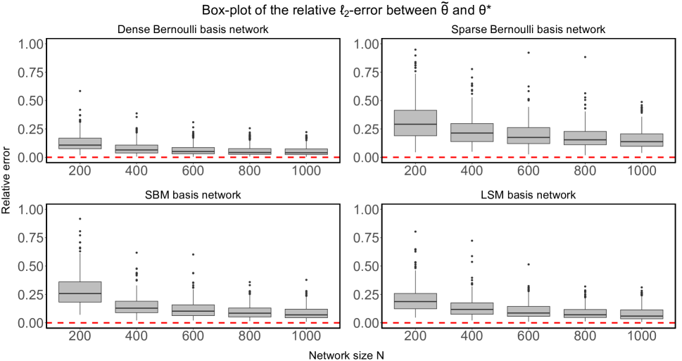
Figure 1: The relative $\ell_{2}$-errors between $\widetilde{\bm{\theta}}$ and $\bm{\theta}^{\star}$ decrease as the network size increases in four basis network structures.

Figure 2: Q-Q plots and $p$-values of six components of $\widetilde{\bm{\theta}}$ estimated from 250 multilayer network samples at size 1000 on the dense Bernoulli basis network. The univariate normal test failed to reject the null hypothesis that each component of $\widetilde{\bm{\theta}}$ is marginally normal at a significance level of $.05$.

5.1 Consistency of MPLE

The consistency of the maximum pseudolikelihood estimator $\widetilde{\bm{\theta}}$ is demonstrated through the decay of the relative $\ell_{2}$-errors between $\widetilde{\bm{\theta}}$ and the data-generating parameter $\bm{\theta}^{\star}$. We generate $M=250$ multilayer networks by $M$ different model-generating parameters at five network sizes from $N=200$ to $1000$. For each network size $N$, type of basis network $\bm{Y}$, and replicate, we sample a network separable multilayer network $\bm{X}$ from (1) using the specification in (5) with the data-generating parameter vector $\bm{\theta}^{\star}$ populated by randomly selecting each component from the uniform distribution on $(-1,1)$. We make the exception that the third and the sixth components $\theta_{3}^{\star}$ and $\theta_{1,3}^{\star}$ are set to $0$. In each replicate, we compute the maximum pseudolikelihood estimator. The results of this simulation study are given in Figure 1, which shows the decay of the relative $\ell_{2}$-errors between $\widetilde{\bm{\theta}}$ and $\bm{\theta}^{\star}$ as the network size increases in four different basis network structures. The broad selection of model-generating parameter values on different basis network structures verifies that Theorem 1 holds in many practical settings.

The top-left subplot of Figure 1 shows a baseline result for a dense Bernoulli basis network with $\mathbb{P}(Y_{i,j}=1)=0.8$ for all $\{i,j\}\subset\mathscr{N}$. As the network size increases from $200$ to $1000$, the relative $\ell_{2}$-errors decrease to $0$. The performance of MPLE on different structures of the basis network $\bm{Y}$ is also studied with results being shown in the rest of the subplots of Figure 1. Basis networks $\bm{Y}$ are generated by a sparse Bernoulli random graph (top-right), by a stochastic block model (SBM, bottom-left), and by a latent space model (LSM, bottom-right). In contrast to the baseline result of the dense Bernoulli random graph, where the basis network is populated with more dyadic connections owing to the fact that the expected number of activated dyads $\mathbb{E}|\!|\bm{Y}|\!|_{1}$ is equal to $.8\,\binom{N}{2}$, the three different basis structures possess fewer connections. A key example is the sparse Bernoulli basis network which has a varying density of $\mathbb{P}(Y_{i,j}=1)=20/N$ for all $\{i,j\}\subset\mathscr{N}$, admitting a reciprocal scaling with the network size $N$ which results in a sparse network with bounded average node degree. The SBM generated networks have 5 blocks where the within-block density is $.5$ and the between-block density is $.05$ for all network sizes simulated. The LSM generated networks follow the specifications of Hoff et al. [2002] with a fixed density parameter of $.6$. We simulate node positions on the plane in $\mathbb{R}^{2}$, where coordinates of the position of each node are randomly generated from the standard normal distribution. In order for SBM and LSM generated basis networks to have a comparable number of effective sample size, the parameters of the SBM and the LSM are chosen so that the expected number of activated dyads $\mathbb{E}|\!|\bm{Y}|\!|_{1}$ in both basis networks is approximately $.24\,\binom{N}{2}$.

5.2 Multivariate normality of MPLE and model selection

Table 1: False discovery rates of four procedures for detecting non-zero effects of 6 model-generating parameters ($\bm{\theta}^{\star}_{1}$, $\bm{\theta}^{\star}_{2}$, $\bm{\theta}^{\star}_{3}$, $\bm{\theta}^{\star}_{4}$, $\bm{\theta}^{\star}_{5}$, $\bm{\theta}^{\star}_{6}$) estimated from 250 multilayer network samples at size 1000 on the dense Bernoulli basis network. All FDRs are smaller than $.05$.

Procedure	$\bm{\theta}^{\star}_{1}$	$\bm{\theta}^{\star}_{2}$	$\bm{\theta}^{\star}_{3}$	$\bm{\theta}^{\star}_{4}$	$\bm{\theta}^{\star}_{5}$	$\bm{\theta}^{\star}_{6}$
Bonferroni	.004	.002	.001	.002	.001	.005
Benjamini-Hochberg	.014	.014	.014	.011	.017	.020
Hochberg	.012	.008	.009	.008	.011	.016
Holm	.010	.008	.006	.008	.007	.013

As stated in Section 4 and Theorem 2, the distribution of the maximum likelihood estimator $\widehat{\bm{\theta}}$ and the maximum pseudolikelihood estimator $\widetilde{\bm{\theta}}$ converge in distribution to a multivariate normal distribution asymptotically. In order to study the quality of the normal approximation—especially for univariate testing which would be used for false discovery control and model selection—we randomly select $6$ of the $250$ data-generating parameter vectors $\bm{\theta}^{\star}$ used to study the consistency results of Theorem 1 in the simulation study conducted in Section 5.1. We then generate $250$ replicates of multilayer network samples by each of these $6$ parameter vectors, using specification (5) on different basis network structures. The multivariate normality of $\widetilde{\bm{\theta}}$ passed Zhou-Shao’s multivariate normal test [Zhou and Shao, 2014], with $p$-values provided in the Appendix G.1 in the supplement to this paper. We visualize the marginal normality of individual component in $\widetilde{\bm{\theta}}$ with a dense Bernoulli basis network in Figure 2, through Q-Q plots of the simulated maximum pseudolikelihood estimators. Univariate tests for normality failed to reject the null hypothesis that each component of $\widetilde{\bm{\theta}}$ is marginally normal at a significance level of $.05$. Additional results studying the multivariate normality of $\widetilde{\bm{\theta}}$ on different basis network structures are provided in Appendix G.1 in the supplement to this paper.

We then implement the multiple testing correction procedures of Bonferroni, Benjamini-Hochberg, Hochberg, and Holm, for the 6 selected model-generating parameter vectors $\bm{\theta}^{\star}$ with 250 replicates to detect components that are significantly different from $0$ while controlling the false discovery rate (FDR) at a family-wise significance level of $\alpha=.05$—recall the third and the sixth component $\theta_{1,3}^{\star}$ and $\theta_{3}^{\star}$ of $\bm{\theta}^{\star}$ are set to $0$ in each simulation replicate. We estimate the FDR of the four procedures by averaging the false discovery proportions from 250 replicates of each of the 6 randomly selected model-generating parameters $\bm{\theta}^{\star}$. We provide the estimated FDRs for $\bm{\theta}^{\star}$ on a dense Bernoulli basis network in Table 1. In addition, we show the receiver operating characteristic (ROC) curves for $\widetilde{\bm{\theta}}$ estimating the 6 selected model-generating parameters in each of the subplot of Figure 3, on four basis network structures. Simulation results suggest that the false discovery rate is controlled below the preset threshold $\alpha$. Different model-generating parameter values affect the trade-off between the sensitivity and the specificity of the model selection. In general, multilayer networks with a larger effective sample size lead to a larger area under the ROC curve which offers a tool to choose appropriate correction procedures and thresholds for model selection in different scenarios. Additional results on the false discovery rate with different basis network structures are provided in Appendix G.2 in the supplement to the paper.

Figure 3: ROC curves for $\widetilde{\bm{\theta}}$ estimated from 250 multilayer network samples at size $1000$ of six model-generating parameters on four different basis networks.

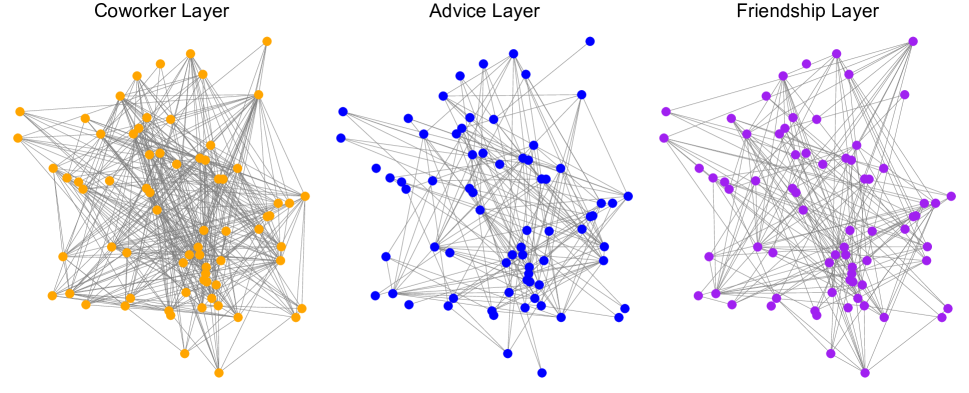
Figure 4: Coworker layer, advice layer and the friendship layer of Lazega’s corporate law partnership network.

Application

Table 2: Summary of Lazega’s corporate law partnership data with 71 lawyers (nodes).

	Average Node Degree	Number of Edges
Co-Worker Layer	11	378
Advice Layer	5	175
Friendship Layer	5	176

We present a case study using a dataset on corporate law partnership among a Northeastern US corporate law firm in New England collected by Lazega [2001]. The dataset collected information about three types of cooperation among 71 lawyers in the corporate law firm, resulting in three networks including the strong-coworker network, the advice network, and the friendship network. Since the cooperation relationship collected are not symmetric, we only consider a connection to be present when both sides acknowledged their cooperation. We treat these three types of networks as a three-layer multilayer network embedded among the 71 lawyers. A summary of this multilayer network is provided in Table 2. We apply model (1) with up to 2-layer interaction terms to the Lazega dataset, i.e., $\bm{\theta}=(\theta_{1},\,\theta_{2},\,\theta_{3},\,\theta_{1,2},\,\theta_{1,3},\,\theta_{2,3})$. The maximum pseudolikelihood estimator $\widetilde{\bm{\theta}}$ is obtained for $\bm{\theta}$ and the results are provided in Table 3.

Table 3: MPLEs for parameters of the Lazega network.

$\widetilde{\theta}_{1}$	$\widetilde{\theta}_{2}$	$\widetilde{\theta}_{3}$	$\widetilde{\theta}_{1,2}$	$\widetilde{\theta}_{1,3}$	$\widetilde{\theta}_{2,3}$	$\mathbb{P}(Y_{i,j}=1)$
$-1.450$	$-3.334$	$-2.695$	$1.801$	$0.218$	$2.458$	0.208
Coworker (C)	Advice (A)	Friendship (F)	C $\times$ A	C $\times$ F	A $\times$ F	Basis network $\bm{Y}$

As shown in Table 3 of the MPLE of the Lazega network data, $\theta_{1},\,\theta_{2}$, and $\theta_{3}$ correspond to single-layer effects of the strong-coworker network, the advice network, and the friendship network, respectively, whereas $\theta_{1,2},\,\theta_{1,3}$, and $\theta_{2,3}$ correspond to the layer interaction effects. We can calculate the conditional log-odds of each edge being present in the multilayer network given the rest of the network. For example, if lawyer $i$ and lawyer $j$ are observed to have an advice relationship and are friends at the same time, the odds of these two lawyers to have a strong-coworker relationship is given by

$$\begin{array}[]{lllllllllllll}\dfrac{\mathbb{P}(X_{i,j}^{(C)}=1\,|\,\bm{X}_{i,j}^{(A)}=1,\,\bm{X}_{i,j}^{(F)}=1)}{\mathbb{P}(X_{i,j}^{(C)}=0\,|\,\bm{X}_{i,j}^{(A)}=1,\,\bm{X}_{i,j}^{(F)}=1)}&=&\exp\left(\theta_{1}+\theta_{1,2}\,x_{i,j}^{(A)}+\theta_{1,3}\,x_{i,j}^{(F)}\right)=1.767,\end{array}$$

providing interpretation of the interaction and influence among the different layers.

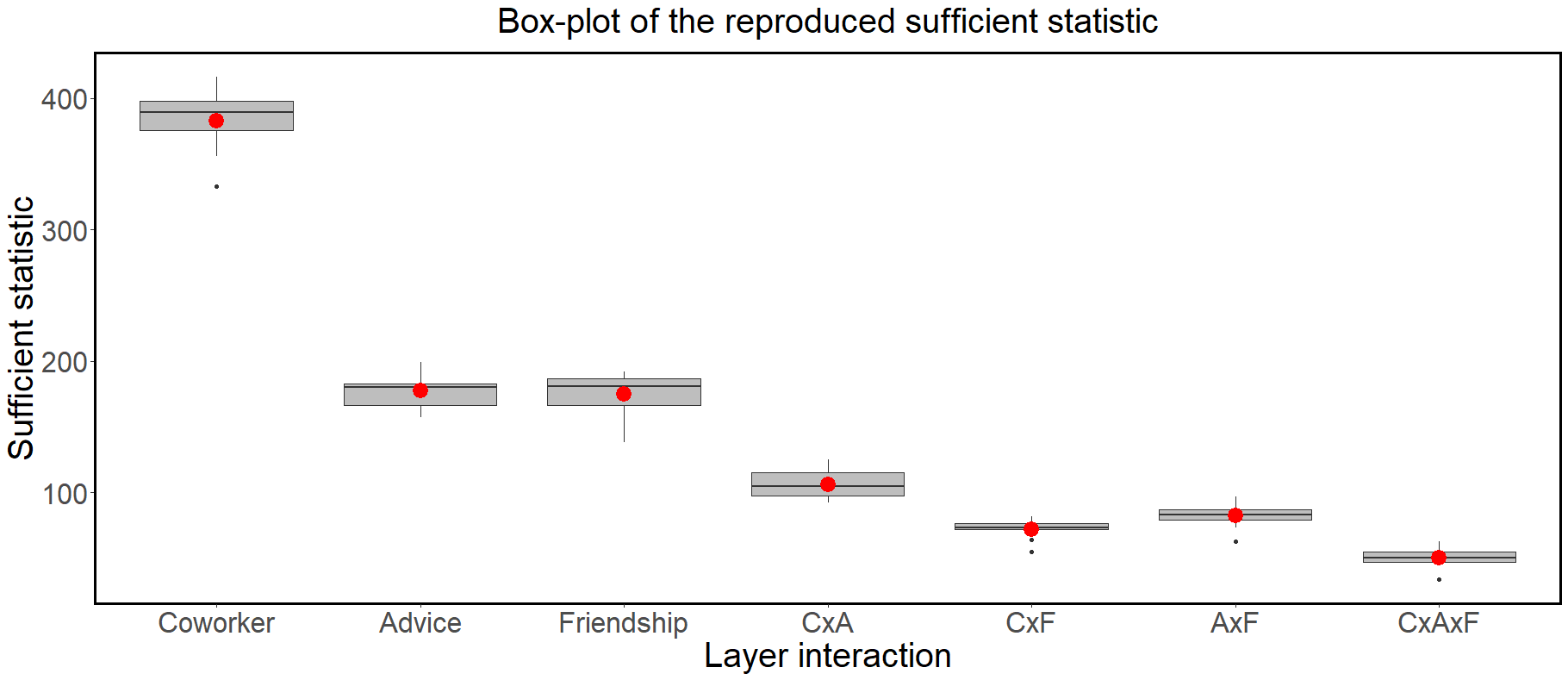
Figure 5: Box-plot of reproduced statistics from 10 replications for each dimension. Red dots are values of the observed sufficient statistics of the Lazega network.

Next, we use the estimated MPLE $\widetilde{\bm{\theta}}$ to simulate networks of the same size and calculate the sufficient statistics of the simulated networks. Comparisons of the sufficient statistics between the observed Lazega network and the simulated networks are provided in Figure 5. Such comparisons serve two key purposes. First, such comparisons are an established method of diagnosing model fit in the statistical network analysis literature [Hunter et al., 2008], and second, provide a check on the approximate solution to the score equation. Note that MPLEs are not guaranteed to reproduce (on average) observed values of sufficient statistics in exponential families—in contrast to MLEs. The relative $\ell_{2}$-error of the sufficient statistics between the observed and the average of 10 simulated networks is $0.013$, suggesting a successful re-construction of the observed network.

Discussion

In this work, we introduced a flexible class of statistical models for multilayer networks. Key to our approach lies in the integrative nature by which we establish our framework, extending arbitrary strictly positive probability distributions for single-layer networks to multilayer-network models through a network separable framework with Markov random field specifications. We established the foundations for statistical inference through consistency and multivariate normality results, the results of which have been demonstrated in simulation studies and in an application. The key assumption to our approach lies in the network separability assumption, which necessitates network dyads be conditionally independent given the basis network. This assumption may or may not be valid in practice, which would necessitate the development of generalizations of the framework we established in this work through the relaxation of the conditional independence assumption. Such relaxations would result in more complex dependence structures, requiring new and careful theoretical treatment in order to establish similar statistical foundations of models to the ones we have developed here, representing potential avenues for future research.

Appendix A: Proof of Proposition 2.1A
Appendix B: Proof of Lemma 1B
Appendix C: Concentration inequalities for multilayer networksC
Appendix D: Proof of Theorem 1D
Appendix E: Proposition E and proofE
Appendix F: Proof of Theorem 2F
Appendix G: Additional simulation resultsG

Appendix A Proof of Proposition 2.1

We prove Proposition 2.1 from Section 2.

Proof of Proposition 2.1. For the first and second results, define the set

$$\begin{array}[]{lllllllllllll}\mathscr{A}_{+}&\coloneqq&\left\{(\bm{x},\bm{y})\in\mathbb{X}\times\mathbb{Y}\;:\;h(\bm{x},\bm{y})=1\right\},\end{array}$$

and the vector-valued map $\bm{\varphi}:\mathbb{X}\mapsto\mathbb{Y}$ by defining its components to be

$$\begin{array}[]{lllllllllllll}\varphi_{i,j}(\bm{x})&=&\mathbbm{1}(|\!|\bm{x}_{i,j}|\!|_{1}>0),&&\{i,j\}\subset\mathscr{N},\end{array}$$

populating the vector $\bm{\varphi}(\bm{x})$ in the lexicographical ordering of the dyad indices $\{i,j\}\subset\mathscr{N}$. By the definition of $h:\mathbb{X}\times\mathbb{Y}\mapsto\{0,1\}$ and $\bm{\varphi}:\mathbb{X}\mapsto\mathbb{Y}$, $\bm{\varphi}(\bm{x})=\bm{y}$ for each pair $(\bm{x},\bm{y})\in\mathscr{A}_{+}$. Furthermore, the element $\bm{y}$ is unique for a given $\bm{x}\in\mathbb{X}$, because if there would exists some $\bm{y}^{\prime}\in\mathbb{Y}$ such that $\bm{y}\neq\bm{y}^{\prime}$ with the property that $\{(\bm{x},\bm{y}),(\bm{x},\bm{y}^{\prime})\}\subseteq\mathscr{A}_{+}$, then there would exist a pair $\{i,j\}\subset\mathscr{N}$ such that $y_{i,j}=1-y^{\prime}_{i,j}$, implying $\mathbbm{1}(|\!|\bm{x}_{i,j}|\!|_{1}>0)\neq y^{\prime}_{i,j}$, in which case $h(\bm{x},\bm{y}^{\prime})=0$, contradicting the assumption that $\{(\bm{x},\bm{y})\}\in\mathscr{A}_{+}$. By (1), the functions $f$ and $g$ are assumed to be strictly positive in their respective domains. Hence, $(\mathbb{X}\times\mathbb{Y})\setminus\mathscr{A}_{+}$ is the largest null set of $\mathbb{X}\times\mathbb{Y}$, i.e., $\mathbb{P}_{\bm{\theta}}(\mathscr{A})=0$ if and only if $\mathscr{A}\subseteq(\mathbb{X}\times\mathbb{Y})\setminus\mathscr{A}_{+}$. Thus, the first and second results are established.

For the third result, note that $g$ is assumed to be strictly positive on its domain $\mathbb{Y}$. Hence, $g(\bm{y})=\mathbb{P}_{\bm{\theta}}(\bm{Y}=\bm{y})>0$ for all $\bm{y}\in\mathbb{Y}$ and $\mathbb{P}_{\bm{\theta}}(\bm{X}=\bm{x}\,|\,\bm{Y}=\bm{y})$ is therefore well-defined. By definition,

$$\begin{array}[]{lllllllllllll}\mathbb{P}_{\bm{\theta}}(\bm{X}=\bm{x}\,|\,\bm{Y}=\bm{y})&=&\dfrac{\mathbb{P}_{\bm{\theta}}(\bm{X}=\bm{x},\,\bm{Y}=\bm{y})}{\mathbb{P}_{\bm{\theta}}(\bm{Y}=\bm{y})},\end{array}$$

where $\mathbb{P}_{\bm{\theta}}(\bm{Y}=\bm{y})$ is the marginal probability of event $\bm{Y}=\bm{y}$ and is assumed to be equal to $g(\bm{y})$. The model form for $\mathbb{P}_{\bm{\theta}}$ given in (1) implies

$$\begin{array}[]{lllllllllllll}\dfrac{\mathbb{P}_{\bm{\theta}}(\bm{X}=\bm{x},\,\bm{Y}=\bm{y})}{\mathbb{P}_{\bm{\theta}}(\bm{Y}=\bm{y})}&=&\dfrac{f(\bm{x},\bm{\theta})\,g(\bm{y})\,\psi(\bm{\theta},\bm{y})}{g(\bm{y})}&=&\exp(\log f(\bm{x},\bm{\theta})+\log\psi(\bm{\theta},\bm{y})),\end{array}$$

under the assumption that $h(\bm{x},\bm{y})=1$. Hence,

$$\begin{array}[]{lllllllllllll}\mathbb{P}_{\bm{\theta}}(\bm{X}=\bm{x},\bm{Y}=\bm{y})&=&\mathbb{P}_{\bm{\theta}}(\bm{X}=\bm{X}\;|\;\bm{Y}=\bm{y})\;\mathbb{P}_{\bm{\theta}}(\bm{Y}=\bm{y})\end{array}$$

so that

$$\begin{array}[]{lllllllllllll}\log\,\mathbb{P}_{\bm{\theta}}(\bm{X}=\bm{x},\bm{Y}=\bm{y})&=&\log\,\mathbb{P}_{\bm{\theta}}(\bm{X}=\bm{X}\;|\;\bm{Y}=\bm{y})+\log\,g(\bm{y}),\end{array}$$

as $g(\bm{y})$ is the marginal probability mass function of $\bm{Y}$, i.e., $\mathbb{P}_{\bm{\theta}}(\bm{Y}=\bm{y})=g(\bm{y})$. Lemma 4 establishes that $\mathbb{P}_{\bm{\theta}}(\bm{X}=\bm{X}\;|\;\bm{Y}=\bm{y})$ belongs to a minimal exponential family, completing the proof of the third and last result of the proposition.

$\hfill\blacksquare$

Appendix B Proof of Lemma 1

We prove Lemma 1 from Section 2.

Proof of Lemma 1. We prove the result in the case of the log-likelihood function. The proof in the case of the log-pseudolikelihood function follows similarly, substituting the appropriate quantities relevant to the log-pseudolikelihood. Using (1),

$$\begin{array}[]{lllllllllllll}-\mathbb{E}\,\nabla_{\bm{\theta}}^{2}\,\ell(\bm{\theta};\bm{X},\bm{Y})&=&\displaystyle\sum\limits_{\bm{y}\in\mathbb{Y}}\,\displaystyle\sum\limits_{\bm{x}\in\mathbb{X}}\,-\nabla_{\bm{\theta}}^{2}\,\ell(\bm{\theta};\bm{x},\bm{y})\,\mathbb{P}_{\bm{\theta}}(\bm{X}=\bm{x}\,|\,\bm{Y}=\bm{y})\,g(\bm{y})\vspace{0.25cm}\\ &=&\displaystyle\sum\limits_{\bm{y}\in\mathbb{Y}}\,g(\bm{y})\displaystyle\sum\limits_{\bm{x}\in\mathbb{X}}\,-\nabla_{\bm{\theta}}^{2}\,\ell(\bm{\theta};\bm{x},\bm{y})\,\mathbb{P}_{\bm{\theta}}(\bm{X}=\bm{x}\,|\,\bm{Y}=\bm{y})\vspace{0.25cm}\\ &=&\displaystyle\sum\limits_{\bm{y}\in\mathbb{Y}}\,g(\bm{y})\,\displaystyle\sum\limits_{\{i,j\}\subset\mathscr{N}\,:\,y_{i,j}=1}\,I(\bm{\theta})\vspace{0.25cm}\\ &=&I(\bm{\theta})\,\displaystyle\sum\limits_{\bm{y}\in\mathbb{Y}}\,g(\bm{y})\,|\!|\bm{y}|\!|_{1}\vspace{0.25cm}\\ &=&I(\bm{\theta})\,\mathbb{E}|\!|\bm{Y}|\!|_{1}.\end{array}$$

The above follows by exploiting the conditional independence of vectors $\bm{x}_{i,j}$ ($\{i,j\}\subset\mathscr{N}$) given $\bm{Y}=\bm{y}$ under (1), which implies

$$\begin{array}[]{lllllllllllll}\ell(\bm{\theta};\bm{x},\bm{y})&=&\displaystyle\sum\limits_{\{i,j\}\subset\mathscr{N}}\log\mathbb{P}_{\bm{\theta}}(\bm{X}_{i,j}=\bm{x}_{i,j}\,|\,\bm{Y}=\bm{y}),\end{array}$$

and from the fact that the conditional probability distribution of $\bm{X}_{i,j}$ given $\bm{Y}$ is a degenerate point mass at $\bm{0}$ when $Y_{i,j}=0$ so that $-\nabla_{\bm{\theta}}^{2}\,\ell(\bm{\theta};\bm{x},\bm{y})$ is a sum of $|\!|\bm{y}|\!|_{1}$ matrices each equal to $I(\bm{\theta})$, i.e., given $\bm{y}\in\mathbb{Y}$, we have

$$\begin{array}[]{lllllllllllll}&&\displaystyle\sum\limits_{\bm{x}\in\mathbb{X}}-\nabla_{\bm{\theta}}^{2}\,\ell(\bm{\theta};\bm{x},\bm{y})\,\mathbb{P}_{\bm{\theta}}(\bm{X}=\bm{x}\,|\,\bm{Y}=\bm{y})\vspace{0.25cm}\\ &=&\displaystyle\sum\limits_{\{i,j\}\subset\mathscr{N}}\,\mathbb{E}\left[-\nabla_{\bm{\theta}}^{2}\,L_{i,j}(\bm{\theta},\bm{X}_{i,j},\bm{Y})\,|\,\bm{Y}=\bm{y}\right]\;\;=\displaystyle\sum\limits_{\{i,j\}\subset\mathscr{N}\,:\,y_{i,j}=1}\,I(\bm{\theta}).\end{array}$$

The fact that $I(\bm{\theta})$ is constant for all pairs $\{i,j\}\subset\mathscr{N}$ satisfying $Y_{i,j}=1$ follows from the form of (1), which assumes each vector $\bm{X}_{i,j}$ ($\{i,j\}\subset\mathscr{N}$) is conditionally independent and identically distributed, conditional on $\bm{Y}$. Hence,

$$\begin{array}[]{lllllllllllll}\mathbb{E}\left[-\nabla_{\bm{\theta}}^{2}\,\ell(\bm{\theta};\bm{X},\bm{Y})\right]&=&I(\bm{\theta})\,\mathbb{E}\,|\!|\bm{Y}|\!|_{1},\end{array}$$

which in turn implies $\lambda_{\min}(-\mathbb{E}\nabla_{\bm{\theta}}^{2}\,\ell(\bm{\theta};\bm{X},\bm{Y}))=\lambda_{\min}(I(\bm{\theta}))\,\mathbb{E}\,|\!|\bm{Y}|\!|_{1}$.

$\hfill\blacksquare$

Appendix C Concentration inequalities for multilayer networks

We establish concentration inequalities of gradients of log-likelihoods and log-pseudolikelihoods functions of network separable multilayer networks in Lemma 2 and Lemma 3, respectively. Recall the definition $[D_{g}]^{+}\coloneqq\max\{0,\,D_{g}\}$, where

$$\begin{array}[]{lllllllllllll}D_{g}&\coloneqq&\displaystyle\sum\limits_{\{i,j\}\prec\{v,w\}\subset\mathscr{N}}\,\mathbb{C}(Y_{i,j},\,Y_{v,w}),\end{array}$$

with $\{i,j\}\prec\{v,w\}$ implying the sum is taken with respect to the lexicographical ordering of pairs of nodes, and where $g:\mathbb{Y}\mapsto(0,1)$ is the marginal probability mass function of $\bm{Y}$.

Lemma 2

Consider multilayer networks satisfying (1) which are defined on a set of $N\geq 3$ nodes and $K\geq 1$ layers. Define $\gamma_{\bm{\theta}}(\bm{x},\bm{y})\coloneqq-\nabla_{\bm{\theta}}\,\ell(\bm{\theta};\bm{x},\bm{y})$, where $\ell(\bm{\theta};\bm{x},\bm{y})$ is the log-likelihood function. Then, for all $t>0$ and $\bm{\theta}\in\mathbb{R}^{p}$,

$$\begin{array}[]{lllllllllllll}\mathbb{P}\left(|\!|\gamma_{\bm{\theta}}(\bm{X},\bm{Y})-\mathbb{E}\,\gamma_{\bm{\theta}}(\bm{X},\bm{Y})|\!|_{\infty}\geq t\right)\;\leq\;2\,\exp\left(-\dfrac{t^{2}}{\mathbb{E}\,|\!|\bm{Y}|\!|_{1}+[D_{g}]^{+}}+\log\,p\right)+\dfrac{1}{\mathbb{E}|\!|\bm{Y}|\!|_{1}}.\end{array}$$

Proof of Lemma 2. By Proposition 2.1,

$$\begin{array}[]{lllllllllllll}\ell(\bm{\theta};\bm{x},\bm{y})&=&\log\,\mathbb{P}_{\bm{\theta}}(\bm{X}=\bm{x}\,|\,\bm{Y}=\bm{y})+\log\,g(\bm{y}).\end{array}$$

Thus,

$$\begin{array}[]{lllllllllllllllll}\nabla_{\bm{\theta}}\,\ell(\bm{\theta};\bm{x},\bm{y})&=&\nabla_{\bm{\theta}}\,\log\,\mathbb{P}_{\bm{\theta}}(\bm{X}=\bm{x}\,|\,\bm{Y}=\bm{y})+\nabla_{\bm{\theta}}\,\log\,g(\bm{y})&=&s(\bm{x})-\mathbb{E}_{\bm{\theta}}\,s(\bm{X}),\end{array}$$ (6)

as $g(\bm{y})=\mathbb{P}_{\bm{\theta}}(\bm{Y}=\bm{y})$ is assumed to not be a function of $\bm{\theta}$. The last equality in (6) follows from Lemma 4, which showed that $\mathbb{P}_{\bm{\theta}}(\bm{X}=\bm{x}\,|\,\bm{Y}=\bm{y})$ is a minimal exponential family with sufficient statistic vector $\bm{s}(\bm{x})$ defined in Lemma 4 and natural parameter vector $\bm{\theta}\in\mathbb{R}^{p}$, inserting the familiar form of the score equation of an exponential family with respect to the natural parameter vector [e.g., Proposition 3.10, p. 32, Sundberg, 2019]. Thus,

$$\begin{array}[]{lllllllllllll}-(\gamma_{\bm{\theta}}(\bm{X},\bm{Y})-\mathbb{E}\,\gamma_{\bm{\theta}}(\bm{X},\bm{Y}))&=&s(\bm{X})-\mathbb{E}_{\bm{\theta}}\,s(\bm{X})-\mathbb{E}\left[s(\bm{X})-\mathbb{E}_{\bm{\theta}}\,s(\bm{X})\right]&=&s(\bm{X})-\mathbb{E}\,s(\bm{X}).\end{array}$$

Let $t>0$ and $\bm{\theta}\in\mathbb{R}^{p}$ be arbitrary and fixed and define $\mathscr{D}_{\infty}(\bm{\theta},t)$ to be the event that $|\!|\gamma_{\bm{\theta}}(\bm{X},\bm{Y})-\mathbb{E}\,\gamma_{\bm{\theta}}(\bm{X},\bm{Y})|\!|_{\infty}=|\!|\bm{s}(\bm{X})-\mathbb{E}\,\bm{s}(\bm{X})|\!|_{\infty}\geq t$. By a union bound,

$$\begin{array}[]{lllllllllllll}\mathbb{P}(|\!|\bm{s}(\bm{X})-\mathbb{E}\,\bm{s}(\bm{X})|\!|_{\infty}\geq t)&=&\mathbb{P}\left(\,\bigcup\limits_{l=1}^{p}\,\Big{[}|s_{l}(\bm{X})-\mathbb{E}\,s_{l}(\bm{X})|\geq t\Big{]}\right)\vspace{0.25cm}\\ &\leq&\displaystyle\sum\limits_{l=1}^{p}\,\mathbb{P}\left(|s_{l}(\bm{X})-\mathbb{E}\,s_{l}(\bm{X})|\geq t\right).\end{array}$$

For each $l\in\{1,\ldots,p\}$, define $\mathscr{D}_{l}(\bm{\theta},t)$ to be the event $|s_{l}(\bm{X})-\mathbb{E}\,s_{l}(\bm{X})|\geq t$. Let $\epsilon>0$ and define $\mathscr{E}(\epsilon)$ to be the event that $||\!|\bm{Y}|\!|_{1}-\mathbb{E}|\!|\bm{Y}|\!|_{1}|\leq\epsilon$, i.e.,

$$\begin{array}[]{lllllllllllll}\mathscr{E}(\epsilon)&=&\left\{\bm{y}\in\mathbb{Y}\,:\,\left||\!|\bm{y}|\!|_{1}-\mathbb{E}|\!|\bm{Y}|\!|_{1}\right|\leq\epsilon\right\}.\end{array}$$

We assume that $\epsilon>0$ is chosen so that $\mathscr{E}(\epsilon)$ is not empty, which implies $\mathbb{P}(\mathscr{E}(\epsilon))>0$ as $g(\bm{y})$ is assumed to be strictly positive on $\mathbb{Y}$. By the law of total probability,

$$\begin{array}[]{lllllllllllllllll}\mathbb{P}\left(\mathscr{D}_{\infty}(\bm{\theta},t)\right)&=&\mathbb{P}\left(\mathscr{D}_{\infty}(\bm{\theta},t)\,|\,\mathscr{E}(\epsilon)\right)\,\mathbb{P}\left(\mathscr{E}(\epsilon)\right)+\mathbb{P}\left(\mathscr{D}_{\infty}(\bm{\theta},t)\,|\,\mathscr{E}(\epsilon)^{c}\right)\,\mathbb{P}\left(\mathscr{E}(\epsilon)^{c}\right)\vspace{0.25cm}\\ &\leq&\mathbb{P}\left(\mathscr{D}_{\infty}(\bm{\theta},t)\,|\,\mathscr{E}(\epsilon)\right)+\mathbb{P}\left(\mathscr{E}(\epsilon)^{c}\right)\vspace{0.25cm}\\ &\leq&\displaystyle\sum\limits_{l=1}^{p}\,\mathbb{P}\left(\mathscr{D}_{l}(\bm{\theta},t)\,|\,\mathscr{E}(\epsilon)\right)+\mathbb{P}\left(\mathscr{E}(\epsilon)^{c}\right).\end{array}$$ (7)

Note that we have not necessarily guaranteed that $\mathbb{P}\left(\mathscr{E}(\epsilon)^{c}\right)>0$. However, if $\mathbb{P}\left(\mathscr{E}(\epsilon)^{c}\right)=0$ the non-conditional form of the law of total probability would yield the bound

$$\begin{array}[]{lllllllllllll}\mathbb{P}\left(\mathscr{D}_{\infty}(\bm{\theta},t)\right)&\leq&\displaystyle\sum\limits_{l=1}^{p}\,\mathbb{P}\left(\mathscr{D}_{l}(\bm{\theta},t)\,|\,\mathscr{E}(\epsilon)\right),\end{array}$$

which is strictly sharper than the bound we give in (7). We will use a divide and conquer strategy to bound each probability in (7) in turn. The form of (1) implies, through factorization principles, that the dyad-based vectors $\bm{X}_{i,j}$ ($\{i,j\}\subset\mathscr{N}$) are conditionally independent given $\bm{Y}$ [e.g., Maathuis et al., 2018, p. 11–13]. Hence, using Lemma 4, the components of the sufficient statistic vector decompose into the sum

$$\begin{array}[]{lllllllllllll}s_{l}(\bm{X})&=&\displaystyle\sum\limits_{\{i,j\}\subset\mathscr{N}}\,s_{l,i,j}(\bm{X}_{i,j}),&&l\in\{1,\ldots,p\},\end{array}$$

so that the components of $\bm{s}(\bm{X})$ are sums of bounded conditionally independent random variables given $\bm{Y}$. Using the forms for $s_{l}(\bm{X})$ and $s_{l,i,j}(\bm{X}_{i,j})$ outlined in Lemma 4, we have $0\leq s_{l,i,j}(\bm{X}_{i,j})\leq Y_{i,j}$ $\mathbb{P}$-almost surely, because $s_{l,i,j}(\bm{X}_{i,j})\in\{0,1\}$ and $s_{l,i,j}(\bm{X}_{i,j})=0$ if $Y_{i,j}=0$ $\mathbb{P}$-almost surely. We may then apply Hoeffding’s inequality to obtain

$$\begin{array}[]{lllllllllllllllll}\mathbb{P}\left(\mathscr{D}_{l}(\bm{\theta},t)\,|\,\bm{Y}=\bm{y}\right)&\leq&2\exp\left(-\dfrac{2\,t^{2}}{|\!|\bm{y}|\!|_{1}}\right),\end{array}$$ (8)

where the denominator follows because $\sum_{\{i,j\}\subset\mathscr{N}}\,y_{i,j}^{2}=|\!|\bm{y}|\!|_{1}$. Using the law of total probability, we bound $\mathbb{P}\left(\mathscr{D}_{l}(\bm{\theta},t)\,|\,\mathscr{E}(\epsilon)\right)$ as follows:

$$\begin{array}[]{lllllllllllllllll}\mathbb{P}\left(\mathscr{D}_{l}(\bm{\theta},t)\,|\,\mathscr{E}(\epsilon)\right)&=&\displaystyle\sum\limits_{\bm{y}\in\mathbb{Y}}\,\mathbb{P}\left(\mathscr{D}_{l}(\bm{\theta},t)\cap[\bm{Y}=\bm{y}]\,|\,\mathscr{E}(\epsilon)\right)\vspace{0.25cm}\\ &=&\displaystyle\sum\limits_{\bm{y}\in\mathscr{E}(\epsilon)}\,\mathbb{P}\left(\mathscr{D}_{l}(\bm{\theta},t)\cap[\bm{Y}=\bm{y}]\,|\,\mathscr{E}(\epsilon)\right)\vspace{0.25cm}\\ &=&\displaystyle\sum\limits_{\bm{y}\in\mathscr{E}(\epsilon)}\,\mathbb{P}\left(\mathscr{D}_{l}(\bm{\theta},t)\,|\,[\bm{Y}=\bm{y}]\cap\mathscr{E}(\epsilon)\right)\,\mathbb{P}(\bm{Y}=\bm{y}\,|\,\mathscr{E}(\epsilon))\vspace{0.25cm}\\ &=&\displaystyle\sum\limits_{\bm{y}\in\mathscr{E}(\epsilon)}\,\mathbb{P}(\mathscr{D}_{l}(\bm{\theta},t)\,|\,\bm{Y}=\bm{y})\,\dfrac{\mathbb{P}(\bm{Y}=\bm{y})}{\mathbb{P}(\mathscr{E}(\epsilon))},\end{array}$$ (9)

noting that $[\bm{Y}=\bm{y}]\cap\mathscr{E}(\epsilon)=[\bm{Y}=\bm{y}]$ whenever $\bm{y}\in\mathscr{E}(\epsilon)$ and in the case when $\bm{y}\not\in\mathscr{E}(\epsilon)$, the intersection is empty, implying

$$\begin{array}[]{lllllllllllll}\mathbb{P}(\bm{Y}=\bm{y}\,|\,\mathscr{E}(\epsilon))&=&\dfrac{\mathbb{P}([\bm{Y}=\bm{y}]\cap\mathscr{E}(\epsilon))}{\mathbb{P}(\mathscr{E}(\epsilon))}&=&\begin{cases}\dfrac{\mathbb{P}(\bm{Y}=\bm{y})}{\mathbb{P}(\mathscr{E}(\epsilon))}&\bm{y}\in\mathscr{E}(\epsilon)\\ 0&\bm{y}\not\in\mathscr{E}(\epsilon)\end{cases}.\end{array}$$

We now bound (9) using the bound in (8):

$$\begin{array}[]{lllllllllllll}\displaystyle\sum\limits_{\bm{y}\in\mathscr{E}(\epsilon)}\,\mathbb{P}(\mathscr{D}_{l}(\bm{\theta},t)\,|\,\bm{Y}=\bm{y})\,\dfrac{\mathbb{P}(\bm{Y}=\bm{y})}{\mathbb{P}(\mathscr{E}(\epsilon))}&\leq&\displaystyle\sum\limits_{\bm{y}\in\mathscr{E}(\epsilon)}\,2\,\exp\left(-\dfrac{2\,t^{2}}{|\!|\bm{y}|\!|_{1}}\right)\,\dfrac{\mathbb{P}(\bm{Y}=\bm{y})}{\mathbb{P}(\mathscr{E}(\epsilon))}\vspace{0.25cm}\\ &\leq&2\,\exp\left(-\dfrac{2\,t^{2}}{\mathbb{E}\,|\!|\bm{Y}|\!|_{1}+\epsilon}\right)\,\displaystyle\sum\limits_{\bm{y}\in\mathscr{E}(\epsilon)}\,\dfrac{\mathbb{P}(\bm{Y}=\bm{y})}{\mathbb{P}(\mathscr{E}(\epsilon))}\vspace{0.25cm}\\ &=&2\,\exp\left(-\dfrac{2\,t^{2}}{\mathbb{E}\,|\!|\bm{Y}|\!|_{1}+\epsilon}\right),\end{array}$$

showing

$$\begin{array}[]{lllllllllllll}\mathbb{P}\left(\mathscr{D}_{l}(\bm{\theta},t)\,|\,\mathscr{E}(\epsilon)\right)&\leq&2\,\exp\left(-\dfrac{2\,t^{2}}{\mathbb{E}\,|\!|\bm{Y}|\!|_{1}+\epsilon}\right).\end{array}$$

The replacement of $|\!|\bm{y}|\!|_{1}$ by $\mathbb{E}|\!|\bm{Y}|\!|_{1}+\epsilon$ follows because $|\!|\bm{y}|\!|_{1}\leq\mathbb{E}|\!|\bm{Y}|\!|_{1}+\epsilon$ for $\bm{y}\in\mathscr{E}(\epsilon)$, resulting in the upper bound above. We bound the second term in the inequality (7) using Chebyshev’s inequality:

$$\begin{array}[]{lllllllllllll}\mathbb{P}(\mathscr{E}(\epsilon)^{c})&=&\mathbb{P}(\left||\!|\bm{Y}|\!|_{1}-\mathbb{E}\,|\!|\bm{Y}|\!|_{1}\right|>\epsilon)&\leq&\mathbb{P}(\left||\!|\bm{Y}|\!|_{1}-\mathbb{E}\,|\!|\bm{Y}|\!|_{1}\right|\geq\epsilon)&\leq&\dfrac{\mathbb{V}(|\!|\bm{Y}|\!|_{1})}{\epsilon^{2}}.\end{array}$$

We bound the variance $\mathbb{V}(|\!|\bm{Y}|\!|_{1})$ as follows:

$$\begin{array}[]{lllllllllllll}\mathbb{V}(|\!|\bm{Y}|\!|_{1})&=&\displaystyle\sum\limits_{\{i,j\}\subset\mathscr{N}}\,\mathbb{V}\,Y_{i,j}+2\,\displaystyle\sum\limits_{\{i,j\}\prec\{v,w\}\subset\mathscr{N}}\,\mathbb{C}(Y_{i,j},\,Y_{v,w})\vspace{0.25cm}\\ &\leq&\mathbb{E}\,|\!|\bm{Y}|\!|_{1}+2\,\displaystyle\sum\limits_{\{i,j\}\prec\{v,w\}\subset\mathscr{N}}\,\mathbb{C}(Y_{i,j},\,Y_{v,w}),\end{array}$$

noting $Y_{i,j}\in\{0,1\}$ so that $\mathbb{V}\,Y_{i,j}=\mathbb{P}(Y_{i,j}=1)\,\mathbb{P}(Y_{i,j}=0)\leq\mathbb{E}\,Y_{i,j}$. Hence,

$$\begin{array}[]{lllllllllllllllll}\mathbb{P}(\mathscr{E}(\epsilon)^{c})&\leq&\dfrac{\mathbb{E}\,|\!|\bm{Y}|\!|_{1}+2\,\sum_{\{i,j\}\prec\{v,w\}\subset\mathscr{N}}\,\mathbb{C}(Y_{i,j},\,Y_{v,w})}{\epsilon^{2}}&=&\dfrac{\mathbb{E}\,|\!|\bm{Y}|\!|_{1}+2\,\left[D_{g}\right]^{+}}{\epsilon^{2}}.\end{array}$$ (10)

Taking $\epsilon=\mathbb{E}\,|\!|\bm{Y}|\!|_{1}+2\,\left[D_{g}\right]^{+}>0$ shows that $\mathbb{P}(\mathscr{E}(\epsilon)^{c})\leq(\mathbb{E}\,|\!|\bm{Y}|\!|_{1})^{-1}$ and

$$\begin{array}[]{lllllllllllll}\mathbb{P}\left(\mathscr{D}_{l}(\bm{\theta},t)\,|\,\mathscr{E}(\epsilon)\right)&\leq&2\,\exp\left(-\dfrac{2\,t^{2}}{2(\mathbb{E}\,|\!|\bm{Y}|\!|_{1}+[D_{g}]^{+})}\right)&=&2\,\exp\left(-\dfrac{t^{2}}{\mathbb{E}\,|\!|\bm{Y}|\!|_{1}+[D_{g}]^{+}}\right).\end{array}$$

Combining all results shows that

$$\begin{array}[]{lllllllllllll}\mathbb{P}\left(|\!|\gamma_{\bm{\theta}}(\bm{X},\bm{Y})-\mathbb{E}\,\gamma_{\bm{\theta}}(\bm{X},\bm{Y})|\!|_{\infty}\geq t\right)\;\leq\;2\,\exp\left(-\dfrac{t^{2}}{\mathbb{E}\,|\!|\bm{Y}|\!|_{1}+[D_{g}]^{+}}+\log\,p\right)+\dfrac{1}{\mathbb{E}|\!|\bm{Y}|\!|_{1}}.\end{array}$$

As a final matter, note that this choice of $\epsilon>0$ ensures $\mathscr{E}(\epsilon)$ contains all $\bm{y}\in\mathbb{Y}$ with $|\!|\bm{y}|\!|_{1}\in[0,\,2(\mathbb{E}\,|\!|\bm{Y}|\!|+[D_{g}]^{+})]$ as the empty graph is an element of $\mathbb{Y}$ with $0$ edges.

$\hfill\blacksquare$

We next prove a related result for gradients of log-pseudolikelihood functions of network separable multilayer networks in Lemma 3. The proof of Lemma 3 essentially follows the same proof of Lemma 2, and as a result we do not repeat key arguments, instead opting to only outline the changes in the proof.

Lemma 3

Consider multilayer networks satisfying (1) which are defined on a set of $N\geq 3$ nodes and $K\geq 1$ layers. Define $\widetilde{\gamma}_{\bm{\theta}}(\bm{x},\bm{y})\coloneqq-\nabla_{\bm{\theta}}\,\widetilde{\ell}(\bm{\theta};\bm{x},\bm{y})$, where $\widetilde{\ell}(\bm{\theta};\bm{x},\bm{y})$ is the log-pseudolikelihood function. Then, for all $t>0$ and $\bm{\theta}\in\mathbb{R}^{p}$,

$$\begin{array}[]{lllllllllllll}\mathbb{P}\left(|\!|\widetilde{\gamma}_{\bm{\theta}}(\bm{X},\bm{Y})-\mathbb{E}\,\widetilde{\gamma}_{\bm{\theta}}(\bm{X},\bm{Y})|\!|_{\infty}\geq t\right)&\leq&2\,\exp\left(-\dfrac{t^{2}}{K^{2}\,(\mathbb{E}\,|\!|\bm{Y}|\!|_{1}+[D_{g}]^{+})}+\log p\right)+\dfrac{1}{\mathbb{E}|\!|\bm{Y}|\!|_{1}}.\end{array}$$

Proof of Lemma 3. From (4), the log-pseudolikelihood function is given by

$$\begin{array}[]{lllllllllllll}\widetilde{\ell}(\bm{\theta};\bm{x},\bm{y})=\displaystyle\sum\limits_{\{i,j\}\subseteq\mathscr{N}}\,\displaystyle\sum\limits_{k=1}^{K}\,\log\,\mathbb{P}_{\bm{\theta}}(X_{i,j}^{(k)}=x_{i,j}^{(k)}\,|\,\bm{X}_{i,j}^{(-k)}=\bm{x}_{i,j}^{(-k)},\bm{Y}=\bm{y}).\end{array}$$

By Lemma 5, $\mathbb{P}_{\bm{\theta}}(X_{i,j}^{(k)}=x_{i,j}^{(k)}\,|\,\bm{X}_{i,j}^{(-k)}=\bm{x}_{i,j}^{(-k)},\bm{Y}=\bm{y})$ is an exponential family with sufficient statistic vector $s:\mathbb{X}\mapsto\mathbb{R}^{p}$ defined in Lemma 4 and natural parameter vector $\bm{\theta}\in\mathbb{R}^{p}$. Hence,

$$\begin{array}[]{lllllllllllll}\nabla_{\bm{\theta}}\,\widetilde{\ell}(\bm{\theta};\bm{x},\bm{y})&=&\displaystyle\sum\limits_{\{i,j\}\subseteq\mathscr{N}}\,\displaystyle\sum\limits_{k=1}^{K}\nabla_{\bm{\theta}}\log\,\mathbb{P}_{\bm{\theta}}(X_{i,j}^{(k)}=x_{i,j}^{(k)}\,|\,\bm{X}_{i,j}^{(-k)}=\bm{x}_{i,j}^{(-k)},\bm{Y}=\bm{y})\vspace{0.25cm}\\ &=&\displaystyle\sum\limits_{\{i,j\}\subseteq\mathscr{N}}\,\displaystyle\sum\limits_{k=1}^{K}\,\left[\,\bm{s}(\bm{x})-\mathbb{E}_{\bm{\theta}}\left[\bm{s}(\bm{X})\,|\,\bm{X}_{i,j}^{-(k)}=\bm{x}_{i,j}^{(-k)},\bm{Y}=\bm{y}\right]\,\right],\end{array}$$

where $\bm{X}_{i,j}^{-(k)}$ denotes the ($K$-$1$)-dimensional vector of edge variables of dyad $\{i,j\}$ in $\bm{X}_{i,j}$ which excludes the single edge variable $X_{i,j}^{(k)}$, and by inserting the familiar form of the score equation of an exponential family with respect to the natural parameter vector [e.g., Proposition 3.10, p. 32, Sundberg, 2019]. Note that $\mathbb{P}_{\bm{\theta}}(X_{i,j}^{(k)}=x_{i,j}^{(k)}\,|\,\bm{X}_{i,j}^{(-k)}=\bm{x}_{i,j}^{(-k)},\bm{Y}=\bm{y})$ may not belong to a minimal exponential family. This presents no issues as we do not require the conditional probability distributions of individual edge variables belong to a minimal exponential family. Under the assumption that $(\bm{X},\bm{Y})$ follow (1), the vectors $\bm{X}_{i,j}$ ($\{i,j\}\subset\mathscr{N}$) are conditionally independent given $\bm{Y}$ (as discussed in the proof of Lemma 2). Therefore, the $l^{th}$ component $s_{l}(\bm{X})$ decomposes into the sum of conditionally independent Bernoulli random variables:

$$\begin{array}[]{lllllllllllll}s_{l}(\bm{X})&=&\displaystyle\sum\limits_{\{i,j\}\subset\mathscr{N}}\,s_{l,i,j}(\bm{X}_{i,j}),&&l\in\{1,\ldots,p\},\end{array}$$

so that the components of $\bm{s}(\bm{X})$ are sums of bounded conditionally independent random variables given $\bm{Y}$. Thus,

$$\begin{array}[]{lllllllllllll}\nabla_{\bm{\theta}}\,\widetilde{\ell}(\bm{\theta};\bm{x},\bm{y})&=&\displaystyle\sum\limits_{\{i,j\}\subseteq\mathscr{N}}\,\displaystyle\sum\limits_{k=1}^{K}\,\left(s_{l,i,j}(\bm{X}_{i,j})-E_{l,i,j}(\bm{\theta},\bm{x}_{i,j},\bm{y})\right),\end{array}$$

where

$$\begin{array}[]{lllllllllllll}E_{l,i,j}(\bm{\theta},\bm{x}_{i,j},\bm{y})&\coloneqq&\mathbb{E}_{\bm{\theta}}\left[s_{l,i,j}(\bm{X}_{i,j})\,|\,\bm{X}_{i,j}^{(-k)}=\bm{x}_{i,j}^{(-k)},\bm{Y}=\bm{y}\right].\end{array}$$

Using the form of $s_{l}(\bm{X})$ and $s_{l,i,j}(\bm{X}_{i,j})$ outlined in Lemma 4, we have $0\leq s_{l,i,j}(\bm{X}_{i,j})\leq Y_{i,j}$ $\mathbb{P}$-almost surely, because $s_{l,i,j}(\bm{X}_{i,j})\in\{0,1\}$ and $s_{l,i,j}(\bm{X}_{i,j})=0$ if $Y_{i,j}=0$ $\mathbb{P}$-almost surely. This also implies $0\leq E_{l,i,j}(\bm{\theta},\bm{x}_{i,j},\bm{y})\leq Y_{i,j}$ $\mathbb{P}$-almost surely. Taken together,

$$\begin{array}[]{lllllllllllll}0\,\leq\,\left|\displaystyle\sum\limits_{k=1}^{K}\,\left(s_{l,i,j}(\bm{X}_{i,j})-E_{l,i,j}(\bm{\theta},\bm{x}_{i,j},\bm{y})\right)\right|\,\leq\,\displaystyle\sum\limits_{k=1}^{K}\left|s_{l,i,j}(\bm{X}_{i,j})-E_{l,i,j}(\bm{\theta},\bm{x}_{i,j},\bm{y})\right|\,\leq\,K\,Y_{i,j},\end{array}$$

$\mathbb{P}$-almost surely. From here, the remainder of the proof follows the proof of Lemma 2, with the sole exception using the bound $K\,Y_{i,j}$ in the application of Hoeffding’s inequality. Reiterating the proof of Lemma 2 with this change will yield

$$\begin{array}[]{lllllllllllll}\mathbb{P}\left(|\!|\widetilde{\gamma}_{\bm{\theta}}(\bm{X},\bm{Y})-\mathbb{E}\,\widetilde{\gamma}_{\bm{\theta}}(\bm{X},\bm{Y})|\!|_{\infty}\geq t\right)&\leq&2\,\exp\left(-\dfrac{t^{2}}{K^{2}\,(\mathbb{E}\,|\!|\bm{Y}|\!|_{1}+[D_{g}]^{+})}+\log p\right)+\dfrac{1}{\mathbb{E}|\!|\bm{Y}|\!|_{1}}.\end{array}$$

$\hfill\blacksquare$

C.1 Auxiliary results

Lemma 4

Consider multilayer networks satisfying (1) with maximum interaction term $H\leq K$ and defined on a set of $N\geq 3$ nodes and $K\geq 1$ layers. Then the following hold:

1. The conditional probability mass function of $\bm{X}$ given $\bm{Y}$ is an exponential family:

   $$\begin{array}[]{lllllllllllll}\mathbb{P}_{\bm{\theta}}(\bm{X}=\bm{x}\mid\bm{Y}=\bm{y})&\propto&h(\bm{x},\,\bm{y})\;\exp\left(\langle\bm{\theta},\,\bm{s}(\bm{x})\rangle\right),\end{array}$$

   where

   $$\begin{array}[]{lllllllllllll}h(\bm{x},\,\bm{y})&=&\displaystyle\prod\limits_{\{i,j\}\subset\mathscr{N}}\,\mathbbm{1}(|\!|\bm{x}_{i,j}|\!|_{1}>0)^{y_{i,j}}\;\mathbbm{1}(|\!|\bm{x}_{i,j}|\!|_{1}=0)^{1-y_{i,j}},\end{array}$$

   sufficient statistic vector $s:\mathbb{X}\mapsto\mathbb{R}^{p}$ and natural parameter vector $\bm{\theta}\in\mathbb{R}^{p}$.

2. For each $l\in\{1,\ldots,p\}$, there exists $h\in\{1,\ldots,H\}$ and $\{k_{1},\ldots,k_{h}\}\subseteq\{1,\ldots,K\}$ such that the $l^{\text{th}}$ component of the sufficient statistic vector $s(\bm{x})$ can be written as

   $$\begin{array}[]{lllllllllllllllll}s_{l}(\bm{x})&=&\displaystyle\sum\limits_{\{i,j\}\subset\mathscr{N}}\,s_{l,i,j}(\bm{x})&=&\displaystyle\prod\limits_{r=1}^{h}\,x_{i,j}^{(k_{r})}.\end{array}$$ (11)

3. The exponential family outlined above is both minimal, full, and regular.

Proof of Lemma 4. First, the form of the conditional probability distribution of $\bm{X}$ given $\bm{Y}$ derived in Proposition 2.1 is given by

$$\begin{array}[]{lllllllllllllllll}\mathbb{P}_{\bm{\theta}}(\bm{X}=\bm{x}\,|\,\bm{Y}=\bm{y})&=&\exp\left(\log\,f(\bm{x},\bm{\theta})+\log\,\psi(\bm{\theta},\bm{y})\right),\end{array}$$ (12)

provided $h(\bm{x},\bm{y})=1$. The form of (1) suggests that (12) will be a minimal exponential family in canonical form due to the form of the Markov random field specification for $f(\bm{\theta},\bm{x})$ and the definition of $\psi(\bm{\theta},\bm{y})$. From the form of $f(\bm{x},\bm{\theta})$ in (1),

$$\begin{array}[]{lllllllllllll}\log f(\bm{x},\bm{\theta})\,=\,\displaystyle\sum\limits_{\{i,j\}\subset\mathscr{N}}\,\left(\displaystyle\sum\limits_{k=1}^{K}\theta_{k}x_{i,j}^{(k)}+\displaystyle\sum\limits_{\begin{subarray}{c}k<l\end{subarray}}^{K}\theta_{k,l}x_{i,j}^{(k)}x_{i,j}^{(l)}+\ldots+\displaystyle\sum\limits_{k_{1}<\ldots<k_{H}}^{K}\theta_{k_{1},k_{2},\ldots,k_{H}}x_{i,j}^{(k_{1})}\cdots x_{i,j}^{(k_{H})}\right),\end{array}$$

where $H\leq K$ is the highest order of cross-layer interactions included in the model. We write $\theta_{k_{1},k_{2},\ldots,k_{h}}$ to reference the $h$-order interaction parameter for the interaction term among layers $\{k_{1},\ldots,k_{h}\}\subseteq\{1,\ldots,K\}$. As specified, $\psi(\bm{\theta},\bm{y})$ is the normalizing constant for the exponential family. As such, the natural parameter space of the exponential family is $\mathbb{R}^{p}$ as the support of $\mathbb{X}$ is finite, which implies $\psi(\bm{\theta},\bm{y})<\infty$ for all $\bm{\theta}\in\mathbb{R}^{p}$ and $\bm{y}\in\mathbb{Y}$. We establish minimality by noting that the components of the parameter vector $\bm{\theta}$ satisfy no linear or affine constraints. Attached to each parameter $\theta_{k_{1},\ldots,k_{h}}$ ($\{k_{1},\ldots,k_{h}\}\subset\{1,\ldots K\}$, $h\in\{1,\ldots,H\}$) is the sufficient statistic

$$\begin{array}[]{lllllllllllll}s_{k_{1},\ldots,k_{h}}(\bm{x})&=&\displaystyle\sum\limits_{\{i,j\}\subset\mathscr{N}}\,x_{i,j}^{(k_{1})}\,\cdots\,x_{i,j}^{(k_{h})}.\end{array}$$

Each statistic $s_{k_{1},\ldots,k_{h}}$ is a function of distinct, non-degenerate random variables, provided $|\!|\bm{y}|\!|_{1}>0$, and so none of the statistics $s_{k_{1},\ldots,k_{h}}$ satisfy any linear or affine constraints. Hence, (1) specifies a minimal and full exponential family with natural parameter space $\mathbb{R}^{p}$ of dimension $p=\sum_{h=1}^{H}\,\binom{K}{h}$ and sufficient statistic vector $s(\bm{x})$ with components $s_{k_{1},\ldots,k_{h}}(\bm{x})$ ($\{k_{1},\ldots,k_{h}\}\subseteq\{1,\ldots,K\},h=1,\ldots,H$). Regularity follows trivially [e.g., Proposition 3.7, pp. 28, Sundberg, 2019]. The form of (11) outlines this for a linear indexing of the components of the sufficient statistic vector.

$\hfill\blacksquare$

Lemma 5

Consider multilayer networks satisfying (1) with maximum interaction term $H\leq K$ and defined on a set of $N\geq 3$ nodes and $K\geq 1$ layers. Then the conditional probability mass function of $X_{i,j}^{(k)}$ given $\bm{Y}=\bm{y}$ and $\bm{X}_{i,j}^{(-k)}=\bm{x}_{i,j}^{(-k)}$ is an exponential family

$$\begin{array}[]{lllllllllllll}\mathbb{P}_{\bm{\theta}}(X_{i,j}^{(k)}=x_{i,j}^{(k)}\,|\,\bm{X}_{i,j}^{(-k)}=\bm{x}_{i,j}^{(-k)},\bm{Y}=\bm{y})&\propto&h(\bm{x},\,\bm{y})\;\exp\left(\langle\bm{\theta},\,\bm{s}(\bm{x})\rangle\right),\end{array}$$

with sufficient statistic vector $\bm{s}:\mathbb{X}\mapsto\mathbb{R}^{p}$ defined in Lemma 4, natural parameter vector $\bm{\theta}\in\mathbb{R}^{p}$, and

$$\begin{array}[]{lllllllllllll}h(\bm{x},\,\bm{y})&=&\displaystyle\prod\limits_{\{i,j\}\subset\mathscr{N}}\,\mathbbm{1}(|\!|\bm{x}_{i,j}|\!|_{1}>0)^{y_{i,j}}\;\mathbbm{1}(|\!|\bm{x}_{i,j}|\!|_{1}=0)^{1-y_{i,j}}.\end{array}$$

Proof of Lemma 5. First, note that the form of (1) and Proposition 2.1 suggests that

$$\begin{array}[]{lllllllllllllllll}\mathbb{P}_{\bm{\theta}}(X_{i,j}^{(k)}=x_{i,j}^{(k)}\,|\,\bm{X}_{i,j}^{(-k)}=\bm{x}_{i,j}^{(-k)},\bm{Y}=\bm{y})\vspace{0.25cm}\\ \quad\quad\quad=\dfrac{h(x_{i,j}^{(k)},\,\bm{x}_{i,j}^{(-k)},\,\bm{y})\;\exp\left(\langle\bm{\theta},\,\bm{s}(x_{i,j}^{(k)},\,\bm{x}_{i,j}^{(-k)})\rangle\right)}{\displaystyle\sum\limits_{x_{i,j}^{(k)}\in\{0,1\}}\,h(x_{i,j}^{(k)},\,\bm{x}_{i,j}^{(-k)},\,\bm{y})\;\exp\left(\langle\bm{\theta},\,\bm{s}(x_{i,j}^{(k)},\,\bm{x}_{i,j}^{(-k)})\rangle\right)}\end{array}$$ (13)

is an exponential family in canonical form using the Markov random field specification for $f(\bm{\theta},\bm{x})$ and the form of the conditional probability distribution of $X_{i,j}^{(k)}$ given $\bm{Y}$ and $\bm{X}_{i,j}^{(-k)}$. However, this exponential family may not be full rank due to possible 0 values of components of the given ($K$-$1$)-dimensional vector $\bm{x}_{i,j}^{(-k)}$ and thus may not be minimal.

$\hfill\blacksquare$

Appendix D Proof of Theorem 1

Proof of Theorem 1. We first prove the theorem for maximum likelihood estimators, and then discuss extensions and changes necessary to prove the result for maximum pseudolikelihood estimators. By Proposition 2.1, observing $\bm{X}=\bm{x}$ implies we observe $\bm{Y}=\bm{y}$, as for each given $\bm{x}\in\mathbb{X}$, $\bm{Y}=\bm{y}$ ($\mathbb{P}$-a.s.) for one and only one $\bm{y}\in\mathbb{Y}$ given by

$$\begin{array}[]{lllllllllllll}y_{i,j}&=&\mathbbm{1}\left(|\!|\bm{x}_{i,j}|\!|_{1}\,>\,0\right),&&\{i,j\}\subset\mathscr{N}.\end{array}$$

Denote the gradient of $-\ell(\bm{\theta};\bm{x},\bm{y})$ by

$$\begin{array}[]{lllllllllllll}\gamma_{\bm{\theta}}(\bm{x},\bm{y})&\coloneqq&-\nabla_{\bm{\theta}}\,\ell(\bm{\theta};\bm{x},\bm{y})\end{array}$$

and the expected Hessian matrix of the negative log-likelihood by

$$\begin{array}[]{lllllllllllll}\bm{H}(\bm{\theta})&\coloneqq&-\mathbb{E}\,\nabla_{\bm{\theta}}^{2}\,\ell(\bm{\theta};\bm{X},\bm{Y}).\end{array}$$

Theorem 6.3.4 of Ortega and Rheinboldt [2000] states that if

$$\begin{array}[]{lllllllllllll}(\bm{\theta}-\bm{\theta}^{\star})^{\top}\,\gamma_{\bm{\theta}}(\bm{x},\bm{y})&\geq&0\end{array}$$

for all $\bm{\theta}\in\partial\,\mathscr{B}_{2}(\bm{\theta}^{\star},\epsilon)$, where $\partial\,\mathscr{B}_{2}(\bm{\theta}^{\star},\epsilon)$ is the boundary of the set

$$\begin{array}[]{lllllllllllll}\mathscr{B}_{2}(\bm{\theta}^{\star},\epsilon)&=&\{\bm{\theta}\in\mathbb{R}^{p}\,:\,|\!|\bm{\theta}-\bm{\theta}^{\star}|\!|_{2}<\epsilon\},\end{array}$$

then $\gamma_{\bm{\theta}}(\bm{x},\bm{y})$ has a root in $\mathscr{B}_{2}(\bm{\theta}^{\star},\epsilon)\cup\partial\mathscr{B}_{2}(\bm{\theta}^{\star},\epsilon)$, i.e., $\widehat{\bm{\theta}}$ exists and satisfies $|\!|\widehat{\bm{\theta}}-\bm{\theta}^{\star}|\!|_{2}\leq\epsilon$. Note that a root of $\gamma_{\bm{\theta}}(\bm{x},\bm{y})$ is also a root of $-\gamma_{\bm{\theta}}(\bm{x},\bm{y})$; in what follows, we consider finding a maximizer of $\ell(\bm{\theta};\bm{x},\bm{y})$ by finding a minimizer of $-\ell(\bm{\theta};\bm{x},\bm{y})$. The classification of roots as maximizers/minimizers is justified from the fact that that $\ell(\bm{\theta};\bm{x},\bm{y})$ is concave in $\bm{\theta}$, a fact which follows from Proposition 2.1, as $g(\bm{y})$ is constant in $\bm{\theta}$ and $\log\,\mathbb{P}_{\bm{\theta}}(\bm{X}=\bm{x}\,|\,\bm{Y}=\bm{y})$ is the log-likelihood of a minimal, full, and regular exponential family with natural parameter vector $\bm{\theta}$ and thus is strictly concave in $\bm{\theta}$ [Proposition 3.10, p. 32, Sundberg, 2019]. By the multivariate mean-value theorem [Furi and Martelli, 1991, Theorem 5],

$$\begin{array}[]{lllllllllllll}(\bm{\theta}-\bm{\theta}^{\star})^{\top}\mathbb{E}\,\gamma_{\bm{\theta}}(\bm{X},\bm{Y})&=&(\bm{\theta}-\bm{\theta}^{\star})^{\top}\mathbb{E}\,\gamma_{\bm{\theta}^{\star}}(\bm{X},\bm{Y})+(\bm{\theta}-\bm{\theta}^{\star})^{\top}\bm{H}(\dot{\bm{\theta}})(\bm{\theta}-\bm{\theta}^{\star})\vspace{0.25cm}\\ &=&(\bm{\theta}-\bm{\theta}^{\star})^{\top}\bm{H}(\dot{\bm{\theta}})(\bm{\theta}-\bm{\theta}^{\star}),\end{array}$$

where $\dot{\bm{\theta}}=t\,\bm{\theta}+(1-t)\,\bm{\theta}^{\star}$ (some $t\in[0,1]$) and by invoking Lemma 2 of Stewart and Schweinberger [2021], which shows that both the expected log-likelihood and log-pseudolikelihood of a minimal exponential family is uniquely maximized at the data-generating parameter vector $\bm{\theta}^{\star}$, implying $\mathbb{E}\,\gamma_{\bm{\theta}^{\star}}(\bm{X},\bm{Y})=0$. Let $\epsilon\in(0,\epsilon^{\star})$ and arbitrarily take $\bm{\theta}\in\partial\mathscr{B}_{2}(\bm{\theta}^{\star},\epsilon)$. Then

$$\begin{array}[]{lllllllllllll}(\bm{\theta}-\bm{\theta}^{\star})^{\top}\bm{H}(\dot{\bm{\theta}})(\bm{\theta}-\bm{\theta}^{\star})=\dfrac{(\bm{\theta}-\bm{\theta}^{\star})^{\top}\bm{H}(\dot{\bm{\theta}})(\bm{\theta}-\bm{\theta}^{\star})}{(\bm{\theta}-\bm{\theta}^{\star})^{\top}(\bm{\theta}-\bm{\theta}^{\star})}|\!|\bm{\theta}-\bm{\theta}^{\star}|\!|_{2}^{2}\,\geq\,\epsilon^{2}\,\lambda_{\min}(\bm{H}(\dot{\bm{\theta}})),\end{array}$$

since $|\!|\bm{\theta}-\bm{\theta}^{\star}|\!|_{2}=\epsilon$ as $\bm{\theta}\in\partial\mathscr{B}_{2}(\bm{\theta}^{\star},\epsilon)$ and because the Rayleigh quotient of a matrix is bounded below by the smallest eigenvalue of that matrix so that

$$\begin{array}[]{lllllllllllll}\dfrac{(\bm{\theta}-\bm{\theta}^{\star})^{\top}\bm{H}(\dot{\bm{\theta}})(\bm{\theta}-\bm{\theta}^{\star})}{(\bm{\theta}-\bm{\theta}^{\star})^{\top}(\bm{\theta}-\bm{\theta}^{\star})}\;\geq\;\lambda_{\min}(\bm{H}(\dot{\bm{\theta}}))\;\geq\;\inf\limits_{\bm{\theta}\in\mathscr{B}_{2}(\bm{\theta}^{\star},\epsilon^{\star})}\,\lambda_{\min}(\bm{H}(\bm{\theta})),\end{array}$$

where $\lambda_{\min}(\bm{H}(\dot{\bm{\theta}}))$ is the smallest eigenvalue of $\bm{H}(\dot{\bm{\theta}})$, noting that

$$\begin{array}[]{lllllllllllll}|\!|\dot{\bm{\theta}}-\bm{\theta}^{\star}|\!|_{2}&=&|\!|t\,\bm{\theta}+(1-t)\,\bm{\theta}^{\star}-\bm{\theta}^{\star}|\!|_{2}&=&t\,|\!|\bm{\theta}-\bm{\theta}^{\star}|\!|_{2}&\leq&|\!|\bm{\theta}-\bm{\theta}^{\star}|\!|_{2}&\leq&\epsilon^{\star},\end{array}$$

since $t\in[0,1]$. Lemma 1 showed that

$$\begin{array}[]{lllllllllllll}\lambda_{\min}(\bm{H}(\bm{\theta}))&=&\lambda_{\min}(I(\bm{\theta}))\;\mathbb{E}\,|\!|\bm{Y}|\!|_{1},\end{array}$$

which in turn implies

$$\begin{array}[]{lllllllllllll}\inf\limits_{\bm{\theta}\in\mathscr{B}_{2}(\bm{\theta}^{\star},\epsilon^{\star})}\,\lambda_{\min}(\bm{H}(\bm{\theta}))&=&\xi_{\epsilon^{\star}}\;\mathbb{E}\,|\!|\bm{Y}|\!|_{1},\end{array}$$

where

$$\begin{array}[]{lllllllllllll}\xi_{\epsilon^{\star}}&\coloneqq&\inf\limits_{\bm{\theta}\in\mathscr{B}_{2}(\bm{\theta}^{\star},\epsilon^{\star})}\,\lambda_{\min}(I(\bm{\theta})),\end{array}$$

with $I(\bm{\theta})$ defined in Lemma 1. Hence, for $\bm{\theta}\in\partial\mathscr{B}_{2}(\bm{\theta}^{\star},\epsilon)$ ($\epsilon\in(0,\epsilon^{\star})$),

$$\begin{array}[]{lllllllllllll}(\bm{\theta}-\bm{\theta}^{\star})^{\top}\mathbb{E}\,\gamma_{\bm{\theta}}(\bm{X},\bm{Y})&\geq&\epsilon^{2}\;\xi_{\epsilon^{\star}}\;\mathbb{E}\,|\!|\bm{Y}|\!|_{1}.\end{array}$$

We next turn to showing

$$\begin{array}[]{lllllllllllll}\mathbb{P}\left(\inf\limits_{\bm{\theta}\in\mathscr{B}_{2}(\bm{\theta}^{\star},\epsilon)}\,(\bm{\theta}-\bm{\theta}^{\star})^{\top}\,\gamma_{\bm{\theta}}(\bm{X},\bm{Y})\,\geq\,0\right)&\geq&1-2\,(\mathbb{E}|\!|\bm{Y}|\!|_{1})^{-1},\end{array}$$

by showing that the event

$$\begin{array}[]{lllllllllllll}\sup\limits_{\bm{\theta}\in\mathscr{B}_{2}(\bm{\theta}^{\star},\epsilon)}\,|(\bm{\theta}-\bm{\theta}^{\star})^{\top}\,(\mathbb{E}\,\gamma_{\bm{\theta}}(\bm{X},\bm{Y})-\gamma_{\bm{\theta}}(\bm{X},\bm{Y}))|\;<\;\epsilon^{2}\;\xi_{\epsilon^{\star}}\;\mathbb{E}\,|\!|\bm{Y}|\!|_{1}\end{array}$$

occurs with probability at least $1-2\,(\mathbb{E}|\!|\bm{Y}|\!|_{1})^{-1}$, in turn implying that the event $|\!|\widehat{\bm{\theta}}-\bm{\theta}^{\star}|\!|_{2}\leq\epsilon$ happens with probability at least $1-2\,(\mathbb{E}|\!|\bm{Y}|\!|_{1})^{-1}$. Applying the Cauchy-Schwarz inequality and utilizing standard vector norm inequalities,

$$\begin{array}[]{lllllllllllll}|(\bm{\theta}-\bm{\theta}^{\star})^{\top}\,(\mathbb{E}\,\gamma_{\bm{\theta}}(\bm{X},\bm{Y})-\gamma_{\bm{\theta}}(\bm{X},\bm{Y}))|&\leq&|\!|\bm{\theta}-\bm{\theta}^{\star}|\!|_{2}\,|\!|\gamma_{\bm{\theta}}(\bm{X},\bm{Y})-\mathbb{E}\,\gamma_{\bm{\theta}}(\bm{X},\bm{Y})|\!|_{2}\vspace{0.25cm}\\ &\leq&\epsilon\;\sqrt{p}\;|\!|\gamma_{\bm{\theta}}(\bm{X},\bm{Y})-\mathbb{E}\,\gamma_{\bm{\theta}}(\bm{X},\bm{Y})|\!|_{\infty},\end{array}$$

noting $\bm{\theta}\in\partial\mathscr{B}_{2}(\bm{\theta}^{\star},\epsilon)$. It suffices to demonstrate, for all $\bm{\theta}\in\partial\mathscr{B}_{2}(\bm{\theta}^{\star},\epsilon)$, that

$$\begin{array}[]{lllllllllllll}\mathbb{P}\left(|\!|\gamma_{\bm{\theta}}(\bm{X},\bm{Y})-\mathbb{E}\,\gamma_{\bm{\theta}}(\bm{X},\bm{Y})|\!|_{\infty}\,<\,\epsilon\,p^{-\frac{1}{2}}\,\xi_{\epsilon^{\star}}\;\mathbb{E}\,|\!|\bm{Y}|\!|_{1}\right)&\geq&1-2\,(\mathbb{E}|\!|\bm{Y}|\!|_{1})^{-1}.\end{array}$$

For ease of presentation, we define $\mathscr{D}_{N,\epsilon,p}$ to be the event

$$\begin{array}[]{lllllllllllll}|\!|\gamma_{\bm{\theta}}(\bm{X},\bm{Y})-\mathbb{E}\,\gamma_{\bm{\theta}}(\bm{X},\bm{Y})|\!|_{\infty}&\geq&\epsilon\,p^{-\frac{1}{2}}\,\xi_{\epsilon^{\star}}\;\mathbb{E}\,|\!|\bm{Y}|\!|_{1}.\end{array}$$

Applying Lemma 2,

$$\begin{array}[]{lllllllllllll}\mathbb{P}\left(\mathscr{D}_{N,\epsilon,p}\right)\;\leq\;2\,\exp\left(-\dfrac{(\epsilon\,\xi_{\epsilon^{\star}}\;\mathbb{E}\,|\!|\bm{Y}|\!|_{1})^{2}}{p\,(\mathbb{E}\,|\!|\bm{Y}|\!|_{1}+[D_{g}]^{+})}+\log\,p\right)+\dfrac{1}{\mathbb{E}|\!|\bm{Y}|\!|_{1}},\end{array}$$

where $[D_{g}]^{+}\coloneqq\max\{0,\,D_{g}\}$, recalling

$$\begin{array}[]{lllllllllllll}D_{g}&\coloneqq&\displaystyle\sum\limits_{\{i,j\}\prec\{v,w\}\subset\mathscr{N}}\,\mathbb{C}(Y_{i,j},\,Y_{v,w}),\end{array}$$

where $\{i,j\}\prec\{v,w\}$ implies the sum is taken with respect to the lexicographical ordering of pairs of nodes. Under the assumption that $\mathbb{E}|\!|\bm{Y}|\!|_{1}\geq 1$,

$$\begin{array}[]{lllllllllllll}2\,\exp\left(-\dfrac{\epsilon^{2}\,\xi_{\epsilon^{\star}}^{2}\,(\mathbb{E}|\!|\bm{Y}|\!|_{1})^{2}}{p\,(\mathbb{E}\,|\!|\bm{Y}|\!|_{1}+[D_{g}]^{+})}+\log\,p\right)&\leq&2\,\exp\left(-\dfrac{\epsilon^{2}\,\xi_{\epsilon^{\star}}^{2}\,\mathbb{E}|\!|\bm{Y}|\!|_{1}}{p\,(1+[D_{g}]^{+})}+\log\,p\right).\end{array}$$

Take

$$\begin{array}[]{lllllllllllll}\epsilon&=&\sqrt{\dfrac{3\,p\,\log N}{\mathbb{E}|\!|\bm{Y}|\!|_{1}}}\;\dfrac{\sqrt{1+[D_{g}]^{+}}}{\xi_{\epsilon^{\star}}}.\end{array}$$

If

$$\begin{array}[]{lllllllllllll}\lim\limits_{N\to\infty}\,\sqrt{\dfrac{3\,p\,\log N}{\mathbb{E}|\!|\bm{Y}|\!|_{1}}}\;\dfrac{\sqrt{1+[D_{g}]^{+}}}{\xi_{\epsilon^{\star}}}&=&0,\end{array}$$

then for $N$ sufficiently large, we will have $\epsilon<\epsilon^{\star}$, which ensures $\epsilon^{\star}$ may be chosen independent of $N$ and $p$. While $\epsilon^{\star}$ can be chosen independent of $N$ and $p$, note that $p$ is expected to be a function of $N$ and thus $\xi_{\epsilon^{\star}}$ will not (in general) be independent of $N$, possibly holding implications for how fast $p$ may grow with $N$ for certain $\bm{\theta}^{\star}$ and $\epsilon^{\star}$. This choice of $\epsilon$ in turn implies

$$\begin{array}[]{lllllllllllll}2\,\exp\left(-\dfrac{\epsilon^{2}\,\xi_{\epsilon^{\star}}^{2}\,\mathbb{E}|\!|\bm{Y}|\!|_{1}}{p\,(1+[D_{g}]^{+})}+\log\,p\right)&=&2\,\exp\left(-3\log N+\log p\right)&\leq&2\,N^{-2},\end{array}$$

under the assumption that $p\leq N$, which ensures $-3\log N+\log p\leq-2\,\log N$. Note that $\mathbb{E}|\!|\bm{Y}|\!|_{1}\leq\binom{N}{2}\leq N^{2}$. We have thus shown, for all $\bm{\theta}\in\partial\mathscr{B}_{2}(\bm{\theta}^{\star},\epsilon)$, that

$$\begin{array}[]{lllllllllllll}\mathbb{P}\left(|\!|\gamma_{\bm{\theta}}(\bm{X},\bm{Y})-\mathbb{E}\,\gamma_{\bm{\theta}}(\bm{X},\bm{Y})|\!|_{\infty}\,\leq\,\epsilon\,p^{-\frac{1}{2}}\,\xi_{\epsilon^{\star}}\;\mathbb{E}\,|\!|\bm{Y}|\!|_{1}\right)&\geq&1-3\,(\mathbb{E}\,|\!|\bm{Y}|\!|_{1})^{-1},\end{array}$$

under the above conditions. As a result, there exists $N_{0}\geq 3$ such that, for all $N\geq N_{0}$ and with probability at least $1-3\,(\mathbb{E}\,|\!|\bm{Y}|\!|_{1})^{-1}$, the set $\widehat{\bm{\Theta}}$ is non-empty and the unique element of the set $\widehat{\bm{\theta}}\in\widehat{\bm{\Theta}}$ satisfies (uniqueness following from minimality, as discussed in Section 3)

$$\begin{array}[]{lllllllllllll}|\!|\widehat{\bm{\theta}}-\bm{\theta}^{\star}|\!|_{2}&\leq&\sqrt{\dfrac{3\,p\,\log N}{\mathbb{E}|\!|\bm{Y}|\!|_{1}}}\;\dfrac{\sqrt{1+[D_{g}]^{+}}}{\xi_{\epsilon^{\star}}}.\end{array}$$

The above proof can be extended to maximum pseudolikelihood estimators by substituting the relevant quantities (e.g., $\widetilde{\xi}_{\epsilon^{\star}}$ for $\xi_{\epsilon^{\star}}$, etc.). The one change of note is that instead of applying the concentration inequality in Lemma 2, we apply the concentration inequality in Lemma 3, which includes an additional factor of $K^{2}$. Following these steps and repeating the above proof will show that there exists $N_{0}\geq 3$ such that, for all $N\geq N_{0}$ and with probability at least $1-3\,(\mathbb{E}\,|\!|\bm{Y}|\!|_{1})^{-1}$, the set $\widetilde{\bm{\Theta}}$ is non-empty and each $\widetilde{\bm{\theta}}\in\widetilde{\bm{\Theta}}$ satisfies

$$\begin{array}[]{lllllllllllll}|\!|\widetilde{\bm{\theta}}-\bm{\theta}^{\star}|\!|_{2}&\leq&\sqrt{\dfrac{3\,p\,K^{2}\,\log N}{\mathbb{E}|\!|\bm{Y}|\!|_{1}}}\;\dfrac{\sqrt{1+[D_{g}]^{+}}}{\widetilde{\xi}_{\epsilon^{\star}}},\end{array}$$

where

$$\begin{array}[]{lllllllllllll}\widetilde{\xi}_{\epsilon^{\star}}&\coloneqq&\inf\limits_{\bm{\theta}\in\mathscr{B}_{2}(\bm{\theta}^{\star},\epsilon^{\star})}\,\lambda_{\min}(\widetilde{I}(\bm{\theta})).\end{array}$$

$\hfill\blacksquare$

Appendix E Proposition E and proof

In order to establish a bound on the error of the multivariate normal approximation for estimators of data-generating parameters, we first establish an error bound on the multivariate normal approximation of a standardization of the sufficient statistic vector $\bm{s}(\bm{X})$ of the exponential family distribution of $\bm{X}$ given $\bm{Y}$, derived in Lemma 4, in Proposition E using a Lyapunov type bound presented in Raič [2019]. Proposition E provides the basis for our normality proof for estimators which we presented in Theorem 2.

Proposition 2 Consider multilayer networks satisfying (1) defined on a set of $N\geq 3$ nodes and $K\geq 1$ layers. Denote by $\bm{s}(\bm{X})\in\mathbb{R}^{p}$ the sufficient statistic vector of the exponential family $\mathbb{P}(\bm{X}=\bm{x}\,|\,\bm{Y}=\bm{y})$ as defined in Lemma 4. Let $\mathbb{E}^{\bm{Y}}$ be the random conditional expectation operator for the distribution of $\bm{X}$ conditional on $\bm{Y}$, and define

$$\begin{array}[]{lllllllllllll}\bm{S}_{\mathscr{N}}&\coloneqq&(I(\bm{\theta}^{\star})\,|\!|\bm{Y}|\!|_{1})^{-1/2}\,(\bm{s}(\bm{X})-\mathbb{E}^{\bm{Y}}\bm{s}(\bm{X}))\vspace{0.25cm}\\ &=&\displaystyle\sum\limits_{\{i,j\}\subset\mathscr{N}}\,(I(\bm{\theta}^{\star})\,|\!|\bm{Y}|\!|_{1})^{-1/2}\,(\bm{s}_{i,j}(\bm{X})-\mathbb{E}^{\bm{Y}}\bm{s}_{i,j}(\bm{X})).\end{array}$$

For any measurable convex set $\mathscr{A}\subset\mathbb{R}^{p}$,

$$\begin{array}[]{lllllllllllll}\left|\,\mathbb{P}(\bm{S}_{\mathscr{N}}\in\mathscr{A})-\Phi(\bm{Z}\in\mathscr{A})\,\right|&\leq&\dfrac{83}{\xi_{\epsilon^{\star}}^{3/2}}\,\sqrt{\dfrac{p^{7/2}}{\mathbb{E}\,|\!|\bm{Y}|\!|_{1}}}+\dfrac{4}{\mathbb{E}\,|\!|\bm{Y}|\!|_{1}}+\dfrac{8\,\left[D_{g}\right]^{+}}{\left(\mathbb{E}\,|\!|\bm{Y}|\!|_{1}\right)^{2}},\end{array}$$

where $\Phi$ is the standard multivariate normal measure and $\bm{Z}\sim\text{MvtNorm}(\bm{0}_{p},\bm{I}_{p})$, where $\bm{0}_{p}$ is the $p$-dimensional vector of zeros and $\bm{I}_{p}$ is the $p\times p$ identity matrix.

Before we prove Proposition E, we introduce a Lyapunov type bound in Lemma 6 provided by Theorem 1 of Raic [Raič, 2019].

Lemma 6

Consider a sequence of $n\geq 1$ independent random vectors $\bm{W}_{i}\in\mathbb{R}^{p}$. Assume that $\mathbb{E}\,\bm{W}_{i}=\bm{0}_{p}$ and $\sum_{i=1}^{n}\,\mathbb{V}\,\bm{W}_{i}=\bm{I}_{p}$ where $\bm{0}_{p}$ is the $p$-dimensional vector of zeros and $\bm{I}_{p}$ is the $p\times p$ identity matrix. Define

$$\begin{array}[]{lllllllllllll}\bm{S}_{n}&=&\displaystyle\sum\limits_{i=1}^{n}\,\bm{W}_{i}\end{array}$$

and let $\bm{Z}$ be the standard multivariate normal variable, i.e., $\bm{Z}\sim\text{MvtNorm}(\bm{0}_{p},\bm{I}_{p})$. Then, for all measurable convex sets $\mathscr{A}\subset\mathbb{R}^{p}$,

$$\begin{array}[]{lllllllllllll}\left|\mathbb{P}(\bm{S}_{n}\in\mathscr{A})-\Phi(\bm{Z}\in\mathscr{A})\right|&\leq&(42\,p^{1/4}+16)\,\displaystyle\sum\limits_{i=1}^{n}\,\mathbb{E}\,|\!|\bm{W}_{i}|\!|_{2}^{3},\end{array}$$

where $\Phi$ is the standard multivariate normal measure.

We now turn to proving Proposition E.

Proof of Proposition E. By Proposition 2.1 and Lemma 4, the conditional distribution of the multilayer network $\bm{X}$ given $\bm{Y}$ follows an exponential family with sufficient statistic vector that can be decomposed into the sum of conditionally independent dyad-based statistics:

$$\begin{array}[]{lllllllllllll}\bm{s}(\bm{X})&=&\displaystyle\sum\limits_{\{i,j\}\subset\mathscr{N}}\,\bm{s}_{i,j}(\bm{X}),\end{array}$$

with the precise formula for $\bm{s}_{i,j}(\bm{X})$ given in Lemma 4. Define

$$\begin{array}[]{lllllllllllll}\bm{S}_{\mathscr{N}}&\coloneqq&(I(\bm{\theta}^{\star})\,|\!|\bm{Y}|\!|_{1})^{-1/2}\,(\bm{s}(\bm{X})-\mathbb{E}^{\bm{Y}}\bm{s}(\bm{X}))\vspace{0.25cm}\\ &=&\displaystyle\sum\limits_{\{i,j\}\subset\mathscr{N}}\,(I(\bm{\theta}^{\star})\,|\!|\bm{Y}|\!|_{1})^{-1/2}\,(\bm{s}_{i,j}(\bm{X})-\mathbb{E}^{\bm{Y}}\bm{s}_{i,j}(\bm{X})),\end{array}$$

where $I(\bm{\theta}^{\star})$ is the Fisher information matrix of a single dyad $X_{i,j}$ for $\{i,j\}\subset\mathscr{N}$ satisfying $Y_{i,j}=1$ (i.e., the subset of activated dyads) evaluated at $\bm{\theta}^{\star}$ per Lemma 1 and where $\mathbb{E}^{\bm{Y}}$ is the random conditional expectation operator with respect to the distribution of $\bm{X}$ conditional on $\bm{Y}$. For $\epsilon>0$ satisfying $\epsilon<\mathbb{E}\,|\!|\bm{Y}|\!|_{1}$, define the event $\mathscr{E}(\epsilon)$ by

$$\begin{array}[]{lllllllllllll}\mathscr{E}(\epsilon)&\coloneqq&\left\{\,\bm{y}\in\mathbb{Y}\,:\,|\!|\bm{y}|\!|_{1}\geq\mathbb{E}|\!|\bm{Y}|\!|_{1}-\epsilon\right\}.\end{array}$$

In words, $\mathscr{E}(\epsilon)$ is the subset of configurations of the single-layer network $\bm{Y}$ which have number of edges equal to at least the expected number of activated dyads $\mathbb{E}\,|\!|\bm{Y}|\!|_{1}$ minus $\epsilon>0$. The restrictions placed on $\epsilon$ ensure that $\mathbb{E}\,|\!|\bm{Y}|\!|_{1}-\epsilon>0$ which implies that $\mathscr{E}(\epsilon)$ will not contain the empty graph which has no edges and that $\mathscr{E}(\epsilon)$ will contain the complete graph with $\binom{N}{2}$ edges as $\mathbb{E}\,|\!|\bm{Y}|\!|_{1}<\binom{N}{2}$ (strict inequality following from the fact that $g(\bm{y})$, the marginal probability mass function of $\bm{Y}$, is assumed to be strictly positive on $\mathbb{Y}$). Hence, $\mathbb{P}(\mathscr{E}(\epsilon))>0$ and $\mathbb{P}(\mathscr{E}(\epsilon)^{c})>0$. Let $\mathscr{A}\subset\mathbb{R}^{p}$ be a measurable convex set. By the law of total probability and the triangle inequality, we have

$$\begin{array}[]{lllllllllllllllll}\left|\,\mathbb{P}(\bm{S}_{\mathscr{N}}\in\mathscr{A})-\Phi(\bm{Z}\in\mathscr{A})\,\right|&\leq&\left|\mathbb{P}(\bm{S}_{n}\in\mathscr{A}\,|\,\mathscr{E}(\epsilon))-\Phi(\bm{Z}\in\mathscr{A})\right|\,\mathbb{P}(\mathscr{E}(\epsilon))\vspace{0.25cm}\\ &&+\;\left|\mathbb{P}(\bm{S}_{n}\in\mathscr{A}\,|\,\mathscr{E}^{c}(\epsilon))-\Phi(\bm{Z}\in\mathscr{A})\right|\,\mathbb{P}(\mathscr{E}^{c}(\epsilon))\vspace{0.25cm}\\ &\leq&\sup\limits_{\bm{y}\in\mathscr{E}(\epsilon)}\,\left|\,\mathbb{P}(\bm{S}_{\mathscr{N}}\in\mathscr{A}\,|\,\bm{Y}=\bm{y})-\Phi(\bm{Z}\in\mathscr{A})\,\right|\;+\;\mathbb{P}(\mathscr{E}^{c}(\epsilon)),\end{array}$$ (14)

noting $\left|\mathbb{P}(\bm{S}_{n}\in\mathscr{A}\,|\,\mathscr{E}^{c}(\epsilon))-\Phi(\bm{Z}\in\mathscr{A})\right|\leq 1$ and $\mathbb{P}(\mathscr{E}(\epsilon))\leq 1$. Taking

$$\begin{array}[]{lllllllllllll}\bm{W}_{i,j}&=&(I(\bm{\theta}^{\star})\,|\!|\bm{Y}|\!|_{1})^{-1/2}\,(\bm{s}_{i,j}(\bm{X})-\mathbb{E}^{\bm{Y}}\,\bm{s}_{i,j}(\bm{X})),\end{array}$$

we have

$$\begin{array}[]{lllllllllllll}\mathbb{E}\,[\bm{W}_{i,j}\,|\,\bm{Y}=\bm{y}]&=&0,\end{array}$$

a result of the tower property of conditional expectation, and

$$\begin{array}[]{lllllllllllll}\mathbb{V}\,\left[\sum_{\{i,j\}\subset\mathscr{N}}\,\bm{W}_{i,j}\,|\,\bm{Y}=\bm{y}\right]&=&\bm{I}_{p},\end{array}$$

which follows from Lemma 1 which establishes that $\mathbb{V}[s_{i,j}(\bm{X})\,|\,\bm{Y}=\bm{y}]=I(\bm{\theta}^{\star})$ when $Y_{i,j}=1$, recalling the form of the Fisher information matrix of exponential families to be the covariance matrix of the sufficient statistic vector [e.g., Proposition 3.10, pp. 32, Sundberg, 2019], and due to the fact that $\mathbb{V}[s_{i,j}(\bm{X})\,|\,\bm{Y}=\bm{y}]=\bm{0}_{p,p}$ when $Y_{i,j}=0$. Applying Lemma 6 to the first term of the summation of (14), for any measurable convex set $\mathscr{A}\subset\mathbb{R}^{p}$,

$$\begin{array}[]{lllllllllllll}\left|\mathbb{P}(\bm{S}_{\mathscr{N}}\in\mathscr{A}\,|\,\bm{Y}=\bm{y})-\Phi(\bm{Z}\in\mathscr{A})\right|&\leq&(42\,p^{1/4}+16)\,\displaystyle\sum\limits_{\{i,j\}\subset\mathscr{N}}\,\mathbb{E}\,\left[|\!|\bm{W}_{i,j}|\!|_{2}^{3}\,|\,\bm{Y}=\bm{y}\right].\end{array}$$

Given $\bm{Y}=\bm{y}$, using standard matrix and vector norm inequalities,

$$\begin{array}[]{lllllllllllll}|\!|\bm{W}_{i,j}|\!|_{2}&=&|\!|(I(\bm{\theta}^{\star})\,|\!|\bm{y}|\!|_{1})^{-1/2}\,(\bm{s}_{i,j}(\bm{X})-\mathbb{E}\,\bm{s}_{i,j}(\bm{X}))|\!|_{2}\vspace{0.25cm}\\ &\leq&|\!|\bm{y}|\!|_{1}^{-1/2}\,|\!|\!|I(\bm{\theta}^{\star})^{-1/2}|\!|\!|_{2}\,|\!|\bm{s}_{i,j}(\bm{X})-\mathbb{E}\,\bm{s}_{i,j}(\bm{X})|\!|_{2}\vspace{0.25cm}\\ &\leq&(|\!|\bm{y}|\!|_{1}\,\xi_{\epsilon^{\star}})^{-1/2}\,p^{1/2}\,y_{i,j},\end{array}$$

where $|\!|\!|\cdot|\!|\!|_{2}$ denotes the spectral norm of a $p\times p$ matrix and

$$\begin{array}[]{lllllllllllll}\xi_{\epsilon^{\star}}&\coloneqq&\inf\limits_{\bm{\theta}\in\mathscr{B}_{2}(\bm{\theta}^{\star},\epsilon^{\star})}\,\lambda_{\min}(I(\bm{\theta})),\end{array}$$

for a given and fixed $\epsilon^{\star}>0$, as defined in Section 3. From proofs of Lemma 2 and 3,

$$\begin{array}[]{lllllllllllll}0&\leq&s_{l,i,j}(\bm{x})&\leq&1,&&\mbox{all }l=1,\ldots,p,\,\{i,j\}\subset\mathscr{N},\end{array}$$

$\mathbb{P}$-almost surely. Hence,

$$\begin{array}[]{lllllllllllll}\mathbb{P}(|\!|\bm{s}_{i,j}(\bm{X})-\mathbb{E}^{\bm{Y}}\bm{s}_{i,j}(\bm{X})|\!|_{\infty}\leq y_{i,j}\,|\,\bm{Y}=\bm{y})&=&1,\end{array}$$

implying (conditional on $\bm{Y}=\bm{y}$)

$$\begin{array}[]{lllllllllllll}|\!|\bm{s}_{i,j}(\bm{X})-\mathbb{E}^{\bm{Y}}\,\bm{s}_{i,j}(\bm{X})|\!|_{2}&\leq&(p\,y_{i,j})^{1/2}&=&p^{1/2}\,y_{i,j},\end{array}$$

$\mathbb{P}$-almost surely. As a result,

$$\begin{array}[]{lllllllllllll}\mathbb{E}\,\left[|\!|\bm{W}_{i,j}|\!|_{2}^{3}\,|\,\bm{Y}=\bm{y}\right]&\leq&(|\!|\bm{y}|\!|_{1}\,\xi_{\epsilon^{\star}})^{-3/2}\,p^{3/2}\,y_{i,j},\end{array}$$

noting that $y_{i,j}^{3}=y_{i,j}\in\{0,1\}$. Using the fact that $42\,p^{1/4}+16\leq 58\,p^{1/4}$ ($p\geq 1$), we have

$$\begin{array}[]{lllllllllllll}(42\,p^{1/4}+16)\,\displaystyle\sum\limits_{\{i,j\}\subset\mathscr{N}}\,\mathbb{E}\,\left[|\!|\bm{W}_{i,j}|\!|_{2}^{3}\,|\,\bm{Y}=\bm{y}\right]&\leq&58\,p^{7/4}\,\displaystyle\sum\limits_{\{i,j\}\subset\mathscr{N}}\,y_{i,j}\,(|\!|\bm{y}|\!|_{1}\,\xi_{\epsilon^{\star}})^{-3/2}\vspace{0.25cm}\\ &=&58\,p^{7/4}\,|\!|\bm{y}|\!|_{1}^{-1/2}\,\xi_{\epsilon_{\star}}^{-3/2}\vspace{0.25cm}\\ &\leq&58\,p^{7/4}\,(\mathbb{E}\,|\!|\bm{Y}|\!|_{1}-\epsilon)^{-1/2}\,\xi_{\epsilon_{\star}}^{-3/2},\end{array}$$

as the conditioning event $\mathscr{E}(\epsilon)$ and choice of $\epsilon$ ensure that $|\!|\bm{y}|\!|_{1}\geq\mathbb{E}|\!|\bm{Y}|\!|_{1}-\epsilon>0$. We bound the second term in (14) by Chebyshev’s inequality using equation (10) in the proof of Lemma 2:

$$\begin{array}[]{lllllllllllll}\mathbb{P}(\mathscr{E}^{c}(\epsilon))&\leq&\dfrac{\mathbb{E}\,|\!|\bm{Y}|\!|_{1}+2\,\left[D_{g}\right]^{+}}{\epsilon^{2}}.\end{array}$$

Taking $\epsilon=2^{-1}\,\mathbb{E}\,|\!|\bm{Y}|\!|_{1}>0$, we have

$$\begin{array}[]{lllllllllllll}\mathbb{P}(\mathscr{E}^{c}(\epsilon))&\leq&\dfrac{4}{\mathbb{E}\,|\!|\bm{Y}|\!|_{1}}+\dfrac{8\,\left[D_{g}\right]^{+}}{\left(\mathbb{E}\,|\!|\bm{Y}|\!|_{1}\right)^{2}}.\end{array}$$

Combining terms, we obtain the bound

$$\begin{array}[]{lllllllllllll}\left|\mathbb{P}(\bm{S}_{\mathscr{N}}\in\mathscr{A})-\Phi(\bm{Z}\in\mathscr{A})\right|&\leq&\dfrac{83}{\xi_{\epsilon^{\star}}^{3/2}}\,\sqrt{\dfrac{p^{7/2}}{\mathbb{E}\,|\!|\bm{Y}|\!|_{1}}}+\dfrac{4}{\mathbb{E}\,|\!|\bm{Y}|\!|_{1}}+\dfrac{8\,\left[D_{g}\right]^{+}}{\left(\mathbb{E}\,|\!|\bm{Y}|\!|_{1}\right)^{2}}.\end{array}$$

$\hfill\blacksquare$

Note that the asymptotic multivariate normality can be established provided

$$\begin{array}[]{lllllllllllll}\lim\limits_{N\to\infty}\,\left[\dfrac{83}{\xi_{\epsilon^{\star}}^{3/2}}\,\sqrt{\dfrac{p^{7/2}}{\mathbb{E}\,|\!|\bm{Y}|\!|_{1}}}+\dfrac{4}{\mathbb{E}\,|\!|\bm{Y}|\!|_{1}}+\dfrac{8\,\left[D_{g}\right]^{+}}{\left(\mathbb{E}\,|\!|\bm{Y}|\!|_{1}\right)^{2}}\right]&=&0,\end{array}$$

resulting in following the asymptotic convergence in distribution:

$$\begin{array}[]{lllllllllllll}\bm{S}_{\mathscr{N}}&\overset{D}{\longrightarrow}&\bm{Z}&\sim&\text{MvtNorm}\left(\textbf{0},\,\bm{I}_{p}\right).\end{array}$$

Appendix F Proof of Theorem 2

Proof of Theorem 2. In order to demonstrate the feasibility of the normal approximation for maximum likelihood estimators $\widehat{\bm{\theta}}$ of $\bm{\theta}^{\star}$, we first start with a standard Taylor expansion of the negative score equation:

$$\begin{array}[]{lllllllllllllllll}-\nabla_{\bm{\theta}}\,\ell(\widehat{\bm{\theta}};\bm{x},\bm{y})&=&-\nabla_{\bm{\theta}}\,\ell(\bm{\theta}^{\star};\bm{x},\bm{y})-\nabla_{\bm{\theta}}^{2}\,\ell(\bm{\theta}^{\star};\bm{x},\bm{y})\,(\widehat{\bm{\theta}}-\bm{\theta}^{\star})-\bm{R},\end{array}$$ (15)

where $\bm{R}\in\mathbb{R}^{p}$ is the vector of remainders given in the Lagrange form. Denoting by $R_{i}$, $(\widehat{\bm{\theta}}-\bm{\theta}^{\star})_{i}$, and $(\nabla_{\bm{\theta}}\,\ell(\bm{\theta};\bm{x},\bm{y}))_{i}$ the $i^{\text{th}}$ component of $\bm{R}$, $(\widehat{\bm{\theta}}-\bm{\theta}^{\star})$, and the score function $\nabla_{\bm{\theta}}\,\ell(\bm{\theta};\bm{x},\bm{y})$, respectively. The remainder term $R_{i}$ ($i=1,\ldots,p$) is given by

$$\begin{array}[]{lllllllllllll}R_{i}&=&\displaystyle\sum\limits_{j=1}^{p}\,\dfrac{1}{2}\,\dfrac{\partial^{2}\,(\nabla_{\bm{\theta}}\,\ell(\dot{\bm{\theta}}_{i};\bm{x},\bm{y}))_{i}}{\partial\,\theta_{j}^{2}}(\widehat{\bm{\theta}}-\bm{\theta}^{\star})_{j}^{2}+\;\displaystyle\sum\limits_{1\leq j<k\leq p}\,\dfrac{\partial^{2}\,(\nabla_{\bm{\theta}}\ell(\dot{\bm{\theta}}_{i};\bm{x},\bm{y}))_{i}}{\partial\,\theta_{j}\,\partial\,\theta_{k}}\,(\widehat{\bm{\theta}}-\bm{\theta}^{\star})_{j}\,(\widehat{\bm{\theta}}-\bm{\theta}^{\star})_{k},\end{array}$$

where $\dot{\bm{\theta}}_{i}=t_{i}\,\widehat{\bm{\theta}}+(1-t_{i})\,\bm{\theta}^{\star}$ (for some $t_{i}\in[0,1]$). By Proposition 2.1,

$$\begin{array}[]{lllllllllllll}\ell(\bm{\theta};\bm{x},\bm{y})&=&\log\,\mathbb{P}_{\bm{\theta}}(\bm{X}=\bm{x}\,|\,\bm{Y}=\bm{y})+\log\,g(\bm{y}).\end{array}$$

By Lemma 4, the probability mass function $\mathbb{P}_{\bm{\theta}}(\bm{X}=\bm{x}\,|\,\bm{Y}=\bm{y})$ belongs to a minimal exponential family with sufficient statistic vector $s(\bm{x})=(s_{1}(\bm{x}),\ldots,s_{p}(\bm{x}))$ given by equation (11) in Lemma 4. We then have,

$$\begin{array}[]{lllllllllllll}&-\nabla_{\bm{\theta}}\,\ell(\bm{\theta};\bm{x},\bm{y})&=&-(s(\bm{x})-\mathbb{E}_{\bm{\theta}}^{\bm{y}}\,s(\bm{X}))\vspace{0.25cm}\\ &-\nabla_{\bm{\theta}}^{2}\,\ell(\bm{\theta};\bm{x},\bm{y})&=&\mathbb{V}_{\bm{\theta}}^{\bm{y}}\,s(\bm{X})\;=\;I(\bm{\theta}^{\star})\,|\!|\bm{y}|\!|_{1},\end{array}$$

where $\mathbb{E}_{\bm{\theta}}^{\bm{y}}$ and $\mathbb{V}_{\bm{\theta}}^{\bm{y}}$ are the conditional expectation and variance operators, respectively, of the conditional distribution of $\bm{X}$ given $\bm{Y}=\bm{y}$, and by using standard formulas for exponential families [e.g., Proposition 3.8, pp. 29, Sundberg, 2019] and the results of Lemma 1. Note $\nabla_{\bm{\theta}}\,\ell(\widehat{\bm{\theta}};\bm{x},\bm{y})=0$, as the maximum likelihood estimator $\widehat{\bm{\theta}}$ solves the score equation by definition. We re-arrange (15) and multiply both sides by $(I(\bm{\theta}^{\star})\,|\!|\bm{Y}|\!|_{1})^{-1/2}$ to obtain

$$\begin{array}[]{lllllllllllllllll}&&(I(\bm{\theta}^{\star})\,|\!|\bm{Y}|\!|_{1})^{1/2}\,(\widehat{\bm{\theta}}-\bm{\theta}^{\star})-\;(I(\bm{\theta}^{\star})\,|\!|\bm{Y}|\!|_{1})^{-1/2}\,\bm{R}\vspace{0.25cm}\\ &=&(I(\bm{\theta}^{\star})\,|\!|\bm{Y}|\!|_{1})^{-1/2}\,(s(\bm{X})-\mathbb{E}^{\bm{Y}}\,s(\bm{X})).\end{array}$$ (16)

Define $\tilde{\bm{R}}\coloneqq(I(\bm{\theta}^{\star})\,|\!|\bm{Y}|\!|_{1})^{-1/2}\,\bm{R}$. Let $\mathscr{A}\subset\mathbb{R}^{p}$ be any measurable convex subset of $\mathbb{R}^{p}$ and $\bm{Z}\sim\text{MvtNorm}(\bm{0}_{p},\,\bm{I}_{p})$. We are interested in bounding the quantity

$$\begin{array}[]{lllllllllllll}\left|\mathbb{P}((I(\bm{\theta}^{\star})\,|\!|\bm{Y}|\!|_{1})^{1/2}\,(\widehat{\bm{\theta}}-\bm{\theta}^{\star})-\tilde{\bm{R}}\in\mathscr{A})-\Phi(\bm{Z}\in\mathscr{A})\right|.\end{array}$$

Then from (LABEL:eq:bridge),

$$\begin{array}[]{lllllllllllll}\mathbb{P}\left((I(\bm{\theta}^{\star})\,|\!|\bm{Y}|\!|_{1})^{1/2}\,(\widehat{\bm{\theta}}-\bm{\theta}^{\star})-\tilde{\bm{R}}\in\mathscr{A}\right)\,=\,\mathbb{P}\big{(}(I(\bm{\theta}^{\star})\,|\!|\bm{Y}|\!|_{1})^{-1/2}\,(s(\bm{X})-\mathbb{E}^{\bm{Y}}\,s(\bm{X}))\in\mathscr{A}\big{)}.\end{array}$$

Applying Proposition E, for all measurable convex sets $\mathscr{A}\subseteq\mathbb{R}^{p}$,

$$\begin{array}[]{lllllllllllll}&&\left|\mathbb{P}\left((I(\bm{\theta}^{\star})\,|\!|\bm{Y}|\!|_{1})^{-1/2}\,(s(\bm{X})-\mathbb{E}^{\bm{Y}}\,s(\bm{X}))\in\mathscr{A}\right)-\Phi(\bm{Z}\in\mathscr{A})\right|\vspace{0.25cm}\\ &\leq&\dfrac{83}{\xi_{\epsilon^{\star}}^{3/2}}\,\sqrt{\dfrac{p^{7/2}}{\mathbb{E}\,|\!|\bm{Y}|\!|_{1}}}+\dfrac{4}{\mathbb{E}\,|\!|\bm{Y}|\!|_{1}}+\dfrac{8\,\left[D_{g}\right]^{+}}{\left(\mathbb{E}\,|\!|\bm{Y}|\!|_{1}\right)^{2}}.\end{array}$$

Hence,

$$\begin{array}[]{lllllllllllll}&&\left|\mathbb{P}((I(\bm{\theta}^{\star})\,|\!|\bm{Y}|\!|_{1})^{1/2}\,(\widehat{\bm{\theta}}-\bm{\theta}^{\star})-\tilde{\bm{R}}\in\mathscr{A})-\Phi(\bm{Z}\in\mathscr{A})\right|\vspace{0.25cm}\\ &\leq&\dfrac{83}{\xi_{\epsilon^{\star}}^{3/2}}\,\sqrt{\dfrac{p^{7/2}}{\mathbb{E}\,|\!|\bm{Y}|\!|_{1}}}+\dfrac{4}{\mathbb{E}\,|\!|\bm{Y}|\!|_{1}}+\dfrac{8\,\left[D_{g}\right]^{+}}{\left(\mathbb{E}\,|\!|\bm{Y}|\!|_{1}\right)^{2}}.\vspace{0.25cm}\end{array}$$

We lastly handle the term $\tilde{\bm{R}}$ by showing that $|\!|\tilde{\bm{R}}|\!|_{2}$ is small with high probability. We first use standard vector/matrix norm inequalities to bound

$$\begin{array}[]{lllllllllllll}|\!|\widetilde{\bm{R}}|\!|_{2}&=&|\!|(I(\bm{\theta}^{\star})\,|\!|\bm{Y}|\!|_{1})^{-1/2}\,\bm{R}|\!|_{2}&\leq&\dfrac{|\!|\!|I(\bm{\theta}^{\star})^{-1/2}|\!|\!|_{2}}{\sqrt{|\!|\bm{Y}|\!|_{1}}}\;|\!|\bm{R}|\!|_{2}&\leq&\dfrac{|\!|\bm{R}|\!|_{2}}{\sqrt{\xi_{\epsilon^{\star}}|\!|\bm{Y}|\!|_{1}}},\end{array}$$

noting that the spectral norm $|\!|\!|I(\bm{\theta}^{\star})^{-1/2}|\!|\!|_{2}$ is equal to the largest eigenvalue of $I(\bm{\theta}^{\star})^{-1/2}$ which will be the reciprocal of the smallest eigenvalue of $I(\bm{\theta}^{\star})^{1/2}$, which is bounded below by $\sqrt{\xi_{\epsilon^{\star}}}$. Using a standard result from the Taylor theorem for functions with multiple variables, if for each $i=1,\ldots,p$, there exists constants $M_{i}>0$ such that

$$\begin{array}[]{lllllllllllll}\sup\limits_{\bm{\theta}\in\mathbb{R}^{p}\,:\,|\!|\bm{\theta}-\bm{\theta}^{\star}|\!|_{1}\leq|\!|\widehat{\bm{\theta}}-\bm{\theta}^{\star}|\!|_{1}}\,\left|\,\dfrac{\partial^{2}(\nabla_{\bm{\theta}}\,\ell(\bm{\theta};\bm{x},\bm{y}))_{i}}{\partial\,\theta_{j}\,\partial\,\theta_{k}}\,\right|&\leq&M_{i},&&1\leq j\leq k\leq p,\end{array}$$

then the Lagrange remainder is bounded above by

$$\begin{array}[]{lllllllllllll}R_{i}&\leq&\dfrac{M_{i}}{2}\,|\!|\widehat{\bm{\theta}}-\bm{\theta}^{\star}|\!|_{1}^{2}\end{array}$$

on the set $\{\bm{\theta}\in\mathbb{R}^{p}:|\!|\bm{\theta}-\bm{\theta}^{\star}|\!|_{1}\leq|\!|\widehat{\bm{\theta}}-\bm{\theta}^{\star}|\!|_{2}\}$. By Lemma 7, conditional on $\bm{Y}=\bm{y}$, we have, for all $i=1,\ldots,p$, the bound $M_{i}\leq 2\,|\!|\bm{y}|\!|_{1}$. Hence,

$$\begin{array}[]{lllllllllllllllll}|\!|\tilde{\bm{R}}|\!|_{2}&\leq&\dfrac{1}{\sqrt{\xi_{\epsilon^{\star}}\,|\!|\bm{y}|\!|_{1}}}\;\sqrt{\displaystyle\sum\limits_{i=1}^{p}\,R_{i}^{2}}&\leq&\dfrac{1}{\sqrt{\xi_{\epsilon^{\star}}\,|\!|\bm{y}|\!|_{1}}}\,\sqrt{\displaystyle\sum\limits_{i=1}^{p}\,|\!|\bm{y}|\!|_{1}^{2}\,|\!|\widehat{\bm{\theta}}-\bm{\theta}^{\star}|\!|_{1}^{4}}\vspace{0.25cm}\vspace{0.25cm}\\ &\leq&\dfrac{1}{\sqrt{\xi_{\epsilon^{\star}}\,|\!|\bm{y}|\!|_{1}}}\,\sqrt{p\,|\!|\bm{y}|\!|_{1}^{2}\,|\!|\widehat{\bm{\theta}}-\bm{\theta}^{\star}|\!|_{1}^{4}}&\leq&\dfrac{\sqrt{p}\,|\!|\bm{y}|\!|_{1}\,|\!|\widehat{\bm{\theta}}-\bm{\theta}^{\star}|\!|_{1}^{2}}{\sqrt{\xi_{\epsilon^{\star}}\,|\!|\bm{y}|\!|_{1}}}\vspace{0.25cm}\vspace{0.25cm}\\ &\leq&\dfrac{\sqrt{p}\,\sqrt{|\!|\bm{y}|\!|_{1}}\,p\,|\!|\widehat{\bm{\theta}}-\bm{\theta}^{\star}|\!|_{2}^{2}}{\sqrt{\xi_{\epsilon^{\star}}}}&\leq&\dfrac{p^{3/2}\,\sqrt{|\!|\bm{y}|\!|_{1}}\,|\!|\widehat{\bm{\theta}}-\bm{\theta}^{\star}|\!|_{2}^{2}}{\sqrt{\xi_{\epsilon^{\star}}}}.\end{array}$$ (17)

By Chebyshev’s inequality—as in the proof of Lemma 2—we can establish that

$$\begin{array}[]{lllllllllllllllll}\mathbb{P}\left(\left||\!|\bm{Y}|\!|_{1}-\mathbb{E}\,|\!|\bm{Y}|\!|_{1}\right|>\dfrac{1}{2}\,\mathbb{E}\,|\!|\bm{Y}|\!|_{1}\right)&\leq&\dfrac{4}{\mathbb{E}\,|\!|\bm{Y}|\!|_{1}}+\dfrac{8\,[D_{g}]^{+}}{(\mathbb{E}\,|\!|\bm{Y}|\!|_{1})^{2}},\end{array}$$ (18)

whereas Theorem 1 established there exists $N_{0}\geq 3$ such that, for all $N\geq N_{0}$, the event

$$\begin{array}[]{lllllllllllllllll}|\!|\widehat{\bm{\theta}}-\bm{\theta}^{\star}|\!|_{2}&\leq&\sqrt{\dfrac{3\,p\,\log N}{\mathbb{E}|\!|\bm{Y}|\!|_{1}}}\;\dfrac{\sqrt{1+[D_{g}]^{+}}}{\xi_{\epsilon^{\star}}},\end{array}$$ (19)

occurs with probability at least $1-3\,(\mathbb{E}\,|\!|\bm{Y}|\!|_{1})^{-1}$. Define $\mathscr{E}_{1}$ to be the event

$$\begin{array}[]{lllllllllllll}||\!|\bm{Y}|\!|_{1}-\mathbb{E}\,|\!|\bm{Y}|\!|_{1}|&\leq&\dfrac{1}{2}\,\mathbb{E}\,|\!|\bm{Y}|\!|_{1}\end{array}$$

and $\mathscr{E}_{2}$ to be the event in (19), and define $\mathcal{R}$ to be the corresponding values of $\tilde{\bm{R}}$ in the event $(\bm{X},\bm{Y})\in\mathscr{E}_{1}\cap\mathscr{E}_{2}$, under which we have the bound

$$\begin{array}[]{lllllllllllllllll}|\!|\tilde{\bm{R}}|\!|_{2}&\leq&\dfrac{p^{3/2}\,\sqrt{|\!|\bm{y}|\!|_{1}}}{\sqrt{\xi_{\epsilon^{\star}}}}\,\dfrac{3\,p\,\log N}{\mathbb{E}|\!|\bm{Y}|\!|_{1}}\;\dfrac{1+[D_{g}]^{+}}{\xi_{\epsilon^{\star}}^{2}}\vspace{0.25cm}\vspace{0.25cm}\\ &=&\dfrac{3\,p^{5/2}\,\sqrt{2\,\mathbb{E}\,|\!|\bm{Y}|\!|_{1}}\,\log\,N}{\mathbb{E}|\!|\bm{Y}|\!|_{1}}\,\dfrac{1+[D_{g}]^{+}}{\xi_{\epsilon^{\star}}^{2}}\vspace{0.25cm}\vspace{0.25cm}\\ &=&\dfrac{3\,\sqrt{2}\,(1+[D_{g}]^{+})}{\xi_{\epsilon^{\star}}^{2}}\;\dfrac{p^{5/2}\,\log N}{\sqrt{\mathbb{E}\,|\!|\bm{Y}|\!|_{1}}}.\end{array}$$ (20)

combining the bounds in (17), (18), and (19) and using the fact that

$$\begin{array}[]{lllllllllllll}|\!|\bm{y}|\!|_{1}&\leq&\mathbb{E}\,|\!|\bm{Y}|\!|_{1}+\dfrac{1}{2}\,\mathbb{E}\,|\!|\bm{Y}|\!|_{1}&\leq&2\,\mathbb{E}\,|\!|\bm{Y}|\!|_{1}\end{array}$$

in the event $\bm{y}\in\mathscr{E}_{1}$. Moreover, a union bound shows that

$$\begin{array}[]{lllllllllllll}\mathbb{P}(\tilde{\bm{R}}\not\in\mathcal{R})&\leq&\dfrac{7}{\mathbb{E}\,|\!|\bm{Y}|\!|_{1}}+\dfrac{8\,[D_{g}]^{+}}{(\mathbb{E}\,|\!|\bm{Y}|\!|_{1})^{2}}.\end{array}$$

Hence,

$$\begin{array}[]{lllllllllllllllll}\mathbb{P}\left(|\!|\tilde{\bm{R}}|\!|_{2}\leq\dfrac{3\,\sqrt{2}\,(1+[D_{g}]^{+})}{\xi_{\epsilon^{\star}}^{2}}\;\dfrac{p^{5/2}\,\log N}{\sqrt{\mathbb{E}\,|\!|\bm{Y}|\!|_{1}}}\right)&\geq&1-\dfrac{7}{\mathbb{E}\,|\!|\bm{Y}|\!|_{1}}-\dfrac{8\,[D_{g}]^{+}}{(\mathbb{E}\,|\!|\bm{Y}|\!|_{1})^{2}}.\end{array}$$ (21)

Taken together, we have shown under the assumptions of Theorem 1 that there exists $N_{0}\geq 3$ such that, for all $N\geq N_{0}$, the error of the multivariate normal approximation

$$\begin{array}[]{lllllllllllll}\left|\mathbb{P}((I(\bm{\theta}^{\star})\,|\!|\bm{Y}|\!|_{1})^{1/2}\,(\widehat{\bm{\theta}}-\bm{\theta}^{\star})-\tilde{\bm{R}}\in\mathscr{A})-\Phi(\bm{Z}\in\mathscr{A})\right|\end{array}$$

is bounded above by

$$\begin{array}[]{lllllllllllll}\dfrac{83}{\xi_{\epsilon^{\star}}^{3/2}}\,\sqrt{\dfrac{p^{7/2}}{\mathbb{E}\,|\!|\bm{Y}|\!|_{1}}}+\dfrac{4}{\mathbb{E}\,|\!|\bm{Y}|\!|_{1}}+\dfrac{8\,\left[D_{g}\right]^{+}}{\left(\mathbb{E}\,|\!|\bm{Y}|\!|_{1}\right)^{2}}\end{array}$$

where $\tilde{\bm{R}}$ satisfies

$$\begin{array}[]{lllllllllllll}\mathbb{P}\left(|\!|\tilde{\bm{R}}|\!|_{2}\leq\dfrac{3\,\sqrt{2}\,(1+[D_{g}]^{+})}{\xi_{\epsilon^{\star}}^{2}}\;\dfrac{p^{5/2}\,\log N}{\sqrt{\mathbb{E}\,|\!|\bm{Y}|\!|_{1}}}\right)&\geq&1-\dfrac{7}{\mathbb{E}\,|\!|\bm{Y}|\!|_{1}}-\dfrac{8\,[D_{g}]^{+}}{(\mathbb{E}\,|\!|\bm{Y}|\!|_{1})^{2}}.\end{array}$$

$\hfill\blacksquare$

F.1 Auxiliary results for proof of Theorem 2

Lemma 7

Consider multilayer networks satisfying (1) defined on a set of $N\geq 3$ nodes and $K\geq 1$ layers and denote by the log-likelihood function by $\ell(\bm{\theta};\bm{x},\bm{y})$. Then, for each $i=1,\ldots,p$ and $\epsilon>0$,

$$\begin{array}[]{lllllllllllll}\sup\limits_{\bm{\theta}\in\mathbb{R}^{p}\,:\,|\!|\bm{\theta}-\bm{\theta}^{\star}|\!|_{2}\leq\epsilon}\quad\left|\dfrac{\partial^{2}\,(\nabla_{\bm{\theta}}\,\ell(\bm{\theta};\bm{x},\bm{y}))_{i}}{\partial\,\theta_{j}\,\partial\,\theta_{k}}\right|&\leq&2\,|\!|\bm{y}|\!|_{1},\end{array}$$

where $(\nabla_{\bm{\theta}}\,\ell(\bm{\theta};\bm{x},\bm{y}))_{i}$ is the $i^{th}$ component of the score function $\nabla_{\bm{\theta}}\,\ell(\bm{\theta};\bm{x},\bm{y})$.

Proof of Lemma 7. By Proposition 2.1, given the observation $\bm{x}$ of $\bm{X}$ (i.e., observation of the event $\bm{X}=\bm{x}$), $\bm{Y}$ is predictable with unique value $\bm{y}\in\mathbb{Y}$ given by the formula in Proposition 2.1, and $(\bm{x},\bm{y})$ is network concordant. Further, by Proposition 2.1

$$\begin{array}[]{lllllllllllll}\ell(\bm{\theta};\bm{x},\bm{y})&=&\log\,\mathbb{P}_{\bm{\theta}}(\bm{X}=\bm{x}\mid\bm{Y}=\bm{y})+\log\,g(\bm{y}),\end{array}$$

where $\log\,\mathbb{P}_{\bm{\theta}}(\bm{X}=\bm{x}|\bm{Y}=\bm{y})$ is the log-likelihood of a minimal, full, and regular exponential family. Thus, the second order derivative of $\ell(\bm{\theta};\bm{x},\bm{y})$ with respect to the $i^{\text{th}}$ and $j^{\text{th}}$ components of $\bm{\theta}$ correspond to the variance (in the case $i=j$) or covariance (in the case of $i\neq j$) of corresponding sufficient statistic(s) of the exponential family [e.g., Proposition 3.8, p. 29, Sundberg, 2019], with sufficient statistics given in Lemma 4. For $\{i,j\}\subseteq\{1,\ldots,p\}$,

$$\begin{array}[]{lllllllllllll}\dfrac{\partial\,(\nabla_{\bm{\theta}}\,\ell(\bm{\theta};\bm{x},\bm{y}))_{i}}{\partial\,\theta_{j}}&=&\dfrac{\partial^{2}\,\ell(\bm{\theta};\bm{x},\bm{y})}{\partial\,\theta_{i}\;\partial\,\theta_{j}}&=&\mathbb{C}_{\bm{\theta}}(s_{i}(\bm{X}),s_{j}(\bm{X})\,|\,\bm{Y}=\bm{y}),\end{array}$$

and when $i=j\in\{1,\ldots,p\}$,

$$\begin{array}[]{lllllllllllll}\dfrac{\partial\,(\nabla_{\bm{\theta}}\,\ell(\bm{\theta};\bm{x},\bm{y}))_{i}}{\partial\,\theta_{i}}&=&\dfrac{\partial^{2}\,\ell(\bm{\theta};\bm{x},\bm{y})}{\partial\,\theta_{i}^{2}}&=&\mathbb{V}_{\bm{\theta}}(s_{i}(\bm{X})\,|\,\bm{Y}=\bm{y}).\end{array}$$

As a result, for $\{i,j\}\subseteq\{1,\ldots,p\}$ and $k\in\{1,\ldots,p\}$,

$$\begin{array}[]{lllllllllllll}\left|\,\dfrac{\partial^{2}\,(\nabla_{\bm{\theta}}\,\ell(\bm{\theta};\bm{x},\bm{y}))_{i}}{\partial\,\theta_{j}\,\partial\,\theta_{k}}\,\right|&=&\left|\,\dfrac{\partial\,\mathbb{C}_{\bm{\theta}}(s_{i}(\bm{X}),s_{j}(\bm{X})\,|\,\bm{Y}=\bm{y})}{\partial\,\theta_{k}}\,\right|,\end{array}$$

and when $i=j\in\{1,\ldots,p\}$ and $k\in\{1,\ldots,p\}$,

$$\begin{array}[]{lllllllllllll}\left|\,\dfrac{\partial^{2}\,(\nabla_{\bm{\theta}}\,\ell(\bm{\theta};\bm{x},\bm{y}))_{i}}{\partial\,\theta_{i}\,\partial\,\theta_{k}}\,\right|&=&\left|\,\dfrac{\partial\,\mathbb{V}_{\bm{\theta}}(s_{i}(\bm{X})\,|\,\bm{Y}=\bm{y})}{\partial\,\theta_{k}}\,\right|.\end{array}$$

By Lemma 4 equation (11), conditional on $\bm{Y}=\bm{y}$, each sufficient statistic $s_{i}(\bm{X})$ ($i\in\{1,\ldots,p\}$) can be decomposed into the sum of conditionally independent statistics of each dyad $\bm{X}_{v,w}$, for $\{v,w\}\subseteq\mathscr{N}$. We can then write

$$\begin{array}[]{lllllllllllll}\mathbb{C}_{\bm{\theta}}(s_{i}(\bm{X}),s_{j}(\bm{X})\,|\,\bm{Y}=\bm{y})&=&\displaystyle\sum\limits_{\{v,w\}\subset\mathscr{N}}\,\mathbb{C}_{\bm{\theta}}(s_{i,v,w}(\bm{X}_{v,w}),\,s_{j,v,w}(\bm{X}_{v,w})\,|\,\bm{Y}=\bm{y}),\end{array}$$

noting that by conditional independence $\mathbb{C}_{\bm{\theta}}(s_{i,v,w}(\bm{X}_{v,w}),s_{j,r,t}(\bm{X}_{r,t})\,|\,\bm{Y}=\bm{y})=0$ whenever $\{r,t\}\neq\{v,w\}$, and when $i=j$, we can write

$$\begin{array}[]{lllllllllllll}\mathbb{V}_{\bm{\theta}}(s_{i}(\bm{X})\,|\,\bm{Y}=\bm{y})&=&\displaystyle\sum\limits_{\{v,w\}\subset\mathscr{N}}\,\mathbb{V}_{\bm{\theta}}(s_{i,v,w}(\bm{X}_{v,w})\,|\,\bm{Y}=\bm{y}),\end{array}$$

again appealing to the conditional independence given $\bm{Y}$ of the random variables $s_{i,v,w}(\bm{X}_{v,w})$ ($\{v,w\}\subset\mathscr{N}$). As a result, for $k\in\{1,\ldots,p\}$, it suffices to show that,

$$\begin{array}[]{lllllllllllll}\left|\,\dfrac{\partial\,\mathbb{C}_{\bm{\theta}}(s_{i,v,w}(\bm{X}_{v,w}),\,s_{j,v,w}(\bm{X}_{v,w})\,|\,\bm{Y}=\bm{y})}{\partial\,\theta_{k}}\,\right|&\leq&2,\end{array}$$

and

$$\begin{array}[]{lllllllllllll}\left|\,\dfrac{\partial\,\mathbb{V}_{\bm{\theta}}(s_{i,v,w}(\bm{X}_{v,w})\,|\,\bm{Y}=\bm{y})}{\partial\,\theta_{k}}\,\right|&\leq&1.\end{array}$$

Recall that the sufficient statistic $s_{i,v,w}(\bm{X})$ ($i=1,\ldots,p$) is defined in Lemma 4 by

$$\begin{array}[]{lllllllllllll}s_{i,v,w}(\bm{X}_{v,w})&=&\displaystyle\prod\limits_{t=1}^{h}\,X_{v,w}^{(k_{t})},&&\{v,w\}\subset\mathscr{N},\end{array}$$

for some $h\in\{1,\ldots,H\}$ and $\{k_{1},\ldots,k_{h}\}\subseteq\{1,\ldots,K\}$. Define the set $S_{i,v,w}$ of components of the sufficient statistic vector $\bm{s}_{v,w}(\bm{X})$ for $\{v,w\}\subset\mathscr{N}$ and $i=1,\ldots,p$ by

$$\begin{array}[]{lllllllllllll}S_{i,v,w}\;\coloneqq\;\left\{\displaystyle\prod\limits_{t=1}^{h^{\prime}}\,X_{v,w}^{(l_{t})}\;:\;\{l_{1},\ldots,l_{h^{\prime}}\}\subset\{k_{1},\ldots,k_{h}\},\;h^{\prime}<h\right\},\end{array}$$

where $h\in\{1,\ldots,H\}$ and $\{k_{1},\ldots,k_{h}\}\subseteq\{1,\ldots,K\}$. The set $S_{i,v,w}$ is the set of components of the sufficient statistic vector $\bm{s}_{v,w}(\bm{X})$ of dyad $\{v,w\}\subset\mathscr{N}$ that have a value of 1 when $s_{i,v,w}(\bm{X})=1$. For the ease of notation, let $I_{S_{i,v,w}}$ be the set of dimension indices whose corresponding components of the sufficient statistic vector $\bm{s}_{v,w}(\bm{X})$ belong to the set $S_{i,v,w}$:

$$\begin{array}[]{lllllllllllll}I_{S_{i,v,w}}\;\coloneqq\;\{j\in\{1,\ldots,p\}\;:\;s_{j,v,w}(\bm{X})\in S_{i,v,w}\}.\end{array}$$

Define the conditional expectation of $s_{i,v,w}(\bm{X})$ given $\bm{Y}=\bm{y}$ for any $i\in\{1,\ldots,p\}$ and $\{v,w\}\subset\mathscr{N}$ by

$$\begin{array}[]{lllllllllllll}P_{i,v,w}(\bm{\theta};\bm{X},\bm{y})\;\coloneqq\;\mathbb{P}_{\bm{\theta}}\,(s_{i,v,w}(\bm{X})=1\,|\,\bm{Y}=\bm{y}).\end{array}$$

For further notation simplicity, denote by $L_{i}$ the set of layer indices $\{k_{1},\ldots,k_{h}\}\subseteq\{1,\ldots,K\}$ that define the $i^{th}$ component $s_{i,v,w}(\bm{X}_{v,w})$ of the sufficient statistic vector $\bm{s}_{v,w}(\bm{X})$ for any $\{v,w\}\subset\mathscr{N}$, $j\in\{1,\ldots,p\}$, and some $h\in\{1,\ldots,H\}$. We then define

$$\begin{array}[]{lllllllllllll}\bm{X}_{v,w}^{(L_{i})}&\coloneqq&\left\{X_{v,w}^{(k_{1})},\ldots,X_{v,w}^{(k_{h})}\right\},&&\bm{X}_{v,w}^{(-L_{i})}\;\coloneqq\;\bm{X}_{v,w}\setminus\bm{X}_{v,w}^{(L_{i})},\end{array}$$

and the corresponding sample space

$$\begin{array}[]{lllllllllllll}\mathbb{X}_{v,w}^{(L_{i})}&\coloneqq&\{0,1\}^{h},&&\mathbb{X}_{v,w}^{(-L_{i})}\;\coloneqq\;\{0,1\}^{H-h},\end{array}$$

for some $h\in\{1,\ldots,H\}$. Then we can write

$$\begin{array}[]{lllllllllllll}P_{i,v,w}(\bm{\theta};\bm{X},\bm{y})&=&\mathbb{P}_{\bm{\theta}}\left(\displaystyle\prod\limits_{l\in L_{i}}\,X_{v,w}^{(l)}=1\,|\,\bm{Y}=\bm{y}\right)\vspace{0.25cm}\\ &=&\dfrac{\displaystyle\sum\limits_{\mathbb{X}_{v,w}^{(-L_{i})}}\,\exp\,\left(\sum_{j\in I_{S_{i,v,w}}}\,\theta_{j}+\sum_{j\in I_{S_{i,v,w}}^{c}}\,\theta_{j}\,s_{j,v,w}(\bm{x})\right)}{\displaystyle\sum\limits_{\mathbb{X}_{v,w}}\,\exp\left(\sum_{j=1}^{p}\,\theta_{j}\,s_{j,v,w}(\bm{x})\right)}.\end{array}$$

Let

$$\begin{array}[]{lllllllllllll}Z(\bm{\theta})&\coloneqq&\displaystyle\sum\limits_{\mathbb{X}_{v,w}}\,\exp\left(\sum_{j=1}^{p}\,\theta_{j}\,s_{j,v,w}(\bm{x})\right),\end{array}$$

and take the derivative of $P_{i,v,w}(\bm{\theta};\bm{x},\bm{y})$ with respect to $\theta_{k}$ for $k=1,\ldots,p$. We have

$$\begin{array}[]{lllllllllllllllll}&\dfrac{\partial\,P_{i,v,w}(\bm{\theta};\bm{X},\bm{y})}{\partial\,\theta_{k}}\vspace{0.25cm}\\ \leq&\dfrac{\displaystyle\sum\limits_{\mathbb{X}_{v,w}^{(-L_{i})}}\,\exp\,\left(\sum_{j\in I_{S_{i,v,w}}}\,\theta_{j}+\sum_{j\in I_{S_{i,v,w}}^{c}}\,\theta_{j}\,s_{j,v,w}(\bm{x})\right)\,\left(Z(\bm{\theta})-\dfrac{\partial\,Z(\bm{\theta})}{\partial\,\theta_{k}}\right)}{Z(\bm{\theta})^{2}}\vspace{0.25cm}\\ =&\dfrac{\displaystyle\sum\limits_{\mathbb{X}_{v,w}^{(-L_{i})}}\,\exp\,\left(\sum_{j\in I_{S_{i,v,w}}}\,\theta_{j}+\sum_{j\in I_{S_{i,v,w}}^{c}}\,\theta_{j}\,s_{j,v,w}(\bm{x})\right)\,\left(\displaystyle\sum\limits_{\mathbb{X}_{v,w}}\,\exp\left(\sum_{j=1}^{p}\,\theta_{j}\,s_{j,v,w}(\bm{x})\right)\,(1-s_{k,v,w}(\bm{x}))\right)}{Z(\bm{\theta})^{2}}\vspace{0.25cm}\\ \leq&\dfrac{\displaystyle\sum\limits_{\mathbb{X}_{v,w}^{(-L_{i})}}\,\exp\,\left(\sum_{j\in I_{S_{i,v,w}}}\,\theta_{j}+\sum_{j\in I_{S_{i,v,w}}^{c}}\,\theta_{j}\,s_{j,v,w}(\bm{x})\right)\,Z(\bm{\theta})}{Z(\bm{\theta})^{2}}\vspace{0.25cm}\\ \leq&1.\end{array}$$ (22)

The first inequality is obtained because $s_{k,v,w}(\bm{x})\leq 1$, and the last inequality is due to the fact that

$$\begin{array}[]{lllllllllllll}\displaystyle\sum\limits_{\mathbb{X}_{v,w}^{(-L_{i})}}\,\exp\,\left(\sum_{j\in I_{S_{i,v,w}}}\,\theta_{j}+\sum_{j\in I_{S_{i,v,w}}^{c}}\,\theta_{j}\,s_{j,v,w}(\bm{x})\right)&\leq&\displaystyle\sum\limits_{\mathbb{X}_{v,w}}\,\exp\left(\sum_{j=1}^{p}\,\theta_{j}\,s_{j,v,w}(\bm{x})\right).\end{array}$$

Now we turn to show the derivative of the conditional variance and covariance of the sufficient statistics of each dyad are bounded. Given $\bm{Y}=\bm{y}$, for all $\{i\}\subset\{1,\ldots,p\}$, $s_{i,v,w}(\bm{X})$ are conditionally independent across $\{v,w\}\subseteq\mathscr{N}$. Then we have

$$\begin{array}[]{lllllllllllll}&\mathbb{C}_{\bm{\theta}}(s_{i,v,w}(\bm{X}_{v,w}),\,s_{j,v,w}(\bm{X}_{v,w})\,|\,\bm{Y}=\bm{y})\vspace{0.25cm}\\ =&\mathbb{E}\,[s_{i,v,w}(\bm{X})\,s_{j,v,w}(\bm{X})\,|\,\bm{Y}=\bm{y}]-\mathbb{E}\,[s_{i,v,w}(\bm{X})\,|\,\bm{Y}=\bm{y}]\,\mathbb{E}\,[s_{j,v,w}(\bm{X})\,|\,\bm{Y}=\bm{y}]\vspace{0.25cm}\\ =&\mathbb{P}_{\bm{\theta}}\,(s_{i,v,w}(\bm{X})=1,s_{j,v,w}(\bm{X})=1\,|\,\bm{Y}=\bm{y})-P_{i,v,w}(\bm{\theta};\bm{X},\bm{y})\,P_{j,v,w}(\bm{\theta};\bm{X},\bm{y})\vspace{0.25cm}\\ =&\mathbb{P}_{\bm{\theta}}\left(\displaystyle\prod\limits_{l\in L_{i}\cup L_{j}}\bm{X}_{v,w}^{(l)}=1\,|\,\bm{Y}=\bm{y}\right)-P_{i,v,w}(\bm{\theta};\bm{X},\bm{y})\,P_{j,v,w}(\bm{\theta};\bm{X},\bm{y}).\end{array}$$

Using the inequality derived in (LABEL:cov_ineq) and suppressing the notation of $\{v,w\}$ and $(\bm{X},\bm{y})$ in $P_{i,v,w}(\bm{\theta};\bm{X},\bm{y})$, the derivative of the covariance with respect to $\theta_{k}$, $k=1,\ldots,p$ is given by

$$\begin{array}[]{lllllllllllll}&\left|\,\dfrac{\partial\,\mathbb{C}_{\bm{\theta}}(s_{i,v,w}(\bm{X}_{v,w}),\,s_{j,v,w}(\bm{X}_{v,w})\,|\,\bm{Y}=\bm{y})}{\partial\,\theta_{k}}\,\right|\vspace{0.25cm}\\ =&\dfrac{\partial\,\mathbb{P}_{\bm{\theta}}\left(\displaystyle\prod\limits_{l\in L_{i}\cup L_{j}}\bm{X}_{v,w}^{(l)}=1\,|\,\bm{Y}=\bm{y}\right)}{\partial\,\theta_{k}}-\dfrac{\partial\,P_{i}(\bm{\theta})}{\partial\,\theta_{k}}\,P_{j}(\bm{\theta})-P_{i}(\bm{\theta})\,\dfrac{\partial\,P_{j}(\bm{\theta})}{\partial\,\theta_{k}}\vspace{0.25cm}\\ \leq&2.\end{array}$$

Using the same inequality and notation in (LABEL:cov_ineq), the derivative of the variance of a Bernoulli random variable $s_{i,v,w}(\bm{X})$ is given by

$$\begin{array}[]{lllllllllllll}\left|\,\dfrac{\partial\,\mathbb{V}_{\bm{\theta}}(s_{i,v,w}(\bm{X}_{v,w})\,|\,\bm{Y}=\bm{y})}{\partial\,\theta_{k}}\,\right|&=&\left|\,\left(1-2\,P_{i}(\bm{\theta})\right)\,\dfrac{\partial\,P_{i}(\bm{\theta})}{\partial\,\theta_{k}}\,\right|&\leq&1.\end{array}$$

Finally, for $\{i,j\}\subseteq\{1,\ldots,p\}$ and $k\in\{1,\ldots,p\}$, we obtain

$$\begin{array}[]{lllllllllllll}\left|\,\dfrac{\partial^{2}\,(\nabla_{\bm{\theta}}\,\ell(\bm{\theta};\bm{x},\bm{y}))_{i}}{\partial\,\theta_{j}\,\partial\,\theta_{k}}\,\right|&=&\left|\,\dfrac{\partial\,\mathbb{C}_{\bm{\theta}}(s_{i}(\bm{X}),s_{j}(\bm{X})\,|\,\bm{Y}=\bm{y})}{\partial\,\theta_{k}}\,\right|\vspace{0.25cm}\\ &\leq&\displaystyle\sum\limits_{\{v,w\}\subset\mathscr{N}}\,\left|\dfrac{\partial\,\mathbb{C}_{\bm{\theta}}(s_{i,v,w}(\bm{X}_{v,w}),\,s_{j,v,w}(\bm{X}_{v,w})\,|\,\bm{Y}=\bm{y})}{\partial\,\theta_{k}}\,\right|\vspace{0.25cm}\\ &\leq&2\,|\!|\bm{y}|\!|_{1}\end{array}$$

due to the fact that $\mathbb{C}_{\bm{\theta}}(s_{i,v,w}(\bm{X}_{v,w}),\,s_{j,v,w}(\bm{X}_{v,w})\,|\,\bm{Y}=\bm{y})=0$ when $Y_{v,w}=0$ for $\{v,w\}\subset\mathscr{N}$. Similarly, $\mathbb{V}_{\bm{\theta}}(s_{i,v,w}(\bm{X}_{i,v,w})\,|\,\bm{Y}=\bm{y})=0$ when $Y_{v,w}=0$ for $\{v,w\}\subset\mathscr{N}$, and when $i=j\in\{1,\ldots,p\}$ and $k\in\{1,\ldots,p\}$, we have

$$\begin{array}[]{lllllllllllll}\left|\,\dfrac{\partial^{2}\,(\nabla_{\bm{\theta}}\,\ell(\bm{\theta};\bm{x},\bm{y}))_{i}}{\partial\,\theta_{i}\,\partial\,\theta_{k}}\,\right|&=&\left|\,\dfrac{\partial\,\mathbb{V}_{\bm{\theta}}(s_{i}(\bm{X})\,|\,\bm{Y}=\bm{y})}{\partial\,\theta_{k}}\,\right|\vspace{0.25cm}\\ &\leq&|\!|\bm{y}|\!|_{1}.\end{array}$$

$\hfill\blacksquare$

Appendix G Additional simulation results

We present additional simulation results that enhance those contained in Section 5.

G.1 Normal approximation with different basis networks

The multivariate normality of $\widetilde{\bm{\theta}}$ is tested by Zhou-Shao’s multivariate normal test [Zhou and Shao, 2014], and the p-values are provided in tabel 4. Q-Q plots of $\widetilde{\bm{\theta}}$ estimated from 6 different model-generating parameters with a dense Bernoulli basis network, a sparse Bernoulli basis network, a stochastic block model (SBM) generated basis network, and a latent space model (LSM) generated basis network are shown in Figure 6, 7, 8 and 9, respectively.

Table 4: P-values of the Zhou-Shao’s test for multivariate normality of $\widetilde{\bm{\theta}}$ for 6 model-generating parameters ($\bm{\theta}^{\star}_{1}$, $\bm{\theta}^{\star}_{2}$, $\bm{\theta}^{\star}_{3}$, $\bm{\theta}^{\star}_{4}$, $\bm{\theta}^{\star}_{5}$, $\bm{\theta}^{\star}_{6}$) estimated from 250 network samples at size 1000 on four basis network structures. All p-values are larger than .1.

Basis network model	$\bm{\theta}^{\star}_{1}$	$\bm{\theta}^{\star}_{2}$	$\bm{\theta}^{\star}_{3}$	$\bm{\theta}^{\star}_{4}$	$\bm{\theta}^{\star}_{5}$	$\bm{\theta}^{\star}_{6}$
Dense Bernoulli	.138	.473	.053	.699	.587	.983
Sparse Bernoulli	.554	.132	.232	.634	.904	.373
SBM	.65	.891	.982	.975	.871	.674
LSM	.859	.831	.5	.227	.613	.409

Figure 6: Q-Q plots and p-values of six components of $\widetilde{\bm{\theta}}$ estimated from 250 multilayer network samples at size 1000 on the dense Bernoulli basis network for 6 model-generating parameters on each row.

Figure 7: Q-Q plots and p-values of six components of $\widetilde{\bm{\theta}}$ estimated from 250 multilayer network samples at size 1000 on the sparse Bernoulli basis network for 6 model-generating parameters on each row.

Figure 8: Q-Q plots and p-values of six components of $\widetilde{\bm{\theta}}$ estimated from 250 multilayer network samples at size 1000 on the SBM generated basis network for 6 model-generating parameters on each row.

Figure 9: Q-Q plots and p-values of six components of $\widetilde{\bm{\theta}}$ estimated from 250 multilayer network samples at size 1000 on the LSM generated basis network for 6 model-generating parameters on each row.

G.2 Additional results on the false discovery rate

The false discovery rate (FDR) of the multiple testing correction procedures of Bonferroni, Benjamini-Hochberg, Hochberg, and Holm to detect non-zero components of $\bm{\theta}^{\star}$ at a family-wise significance level of $\alpha=0.05$ with a sparse Bernoulli basis network, an SBM generated basis network and an LSM generated basis network are provided in Table 5, 6 and 7, respectively (recall that the third and the sixth component $\theta_{1,3}^{\star}$ and $\theta_{3}^{\star}$ of $\bm{\theta}^{\star}$ are set to 0).

Table 5: False discovery rates of four procedures for detecting non-zero effects of six model-generating parameters ($\bm{\theta}^{\star}_{1}$, $\bm{\theta}^{\star}_{2}$, $\bm{\theta}^{\star}_{3}$, $\bm{\theta}^{\star}_{4}$, $\bm{\theta}^{\star}_{5}$, $\bm{\theta}^{\star}_{6}$) estimated from 250 multilayer network samples at size 1000 on the sparse Bernoulli basis network. All FDRs are smaller than 0.05.

Procedure	$\bm{\theta}^{\star}_{1}$	$\bm{\theta}^{\star}_{2}$	$\bm{\theta}^{\star}_{3}$	$\bm{\theta}^{\star}_{4}$	$\bm{\theta}^{\star}_{5}$	$\bm{\theta}^{\star}_{6}$
Bonferroni	.002	.003	.003	.003	.003	.011
Benjamini-Hochberg	.020	.011	.022	.022	.014	.017
Hochberg’s	.009	.008	.012	.010	.010	.014
Holm’s	.007	.008	.011	.009	.006	.014

Table 6: False discovery rates of four procedures for detecting non-zero effects of six model-generating parameters ($\bm{\theta}^{\star}_{1}$, $\bm{\theta}^{\star}_{2}$, $\bm{\theta}^{\star}_{3}$, $\bm{\theta}^{\star}_{4}$, $\bm{\theta}^{\star}_{5}$, $\bm{\theta}^{\star}_{6}$) estimated from 250 multilayer network samples at size 1000 on the SBM generated basis network. All FDRs are smaller than 0.05.

Procedure	$\bm{\theta}^{\star}_{1}$	$\bm{\theta}^{\star}_{2}$	$\bm{\theta}^{\star}_{3}$	$\bm{\theta}^{\star}_{4}$	$\bm{\theta}^{\star}_{5}$	$\bm{\theta}^{\star}_{6}$
Bonferroni	.002	.002	.003	.001	.001	.004
Benjamini-Hochberg	.022	.013	.014	.015	.015	.018
Hochberg’s	.009	.014	.01	.008	.011	.014
Holm’s	.009	.013	.005	.009	.009	.011

Table 7: False discovery rates of four procedures for detecting non-zero effects of six model-generating parameters ($\bm{\theta}^{\star}_{1}$, $\bm{\theta}^{\star}_{2}$, $\bm{\theta}^{\star}_{3}$, $\bm{\theta}^{\star}_{4}$, $\bm{\theta}^{\star}_{5}$, $\bm{\theta}^{\star}_{6}$) estimated from 250 multilayer network samples at size 1000 on the LSM generated basis network. All FDRs are smaller than 0.05.

Procedure	$\bm{\theta}^{\star}_{1}$	$\bm{\theta}^{\star}_{2}$	$\bm{\theta}^{\star}_{3}$	$\bm{\theta}^{\star}_{4}$	$\bm{\theta}^{\star}_{5}$	$\bm{\theta}^{\star}_{6}$
Bonferroni	.004	.006	.000	.005	.003	.004
Benjamini-Hochberg	.016	.013	.011	.015	.016	.017
Hochberg’s	.009	.014	.009	.011	.010	.011
Holm’s	.008	.014	.009	.011	.007	.010

References

- Airoldi et al. [2008] E. Airoldi, D. Blei, S. Fienberg, and E. Xing. Mixed membership stochastic blockmodels. Journal of Machine Learning Research, 9:1981–2014, 2008.
- Albert and Barabási [2002] R. Albert and A. L. Barabási. Statistical mechanics of complex networks. Reviews of Modern Physics, 74(1):47, 2002.
- Arroyo et al. [2021] J. A. Arroyo, A. Athreya, J. Cape, G. Chen, C. E. Priebe, and J. T. Vogelstein. Inference for multiple heterogeneous networks with a common invariant subspace. The Journal of Machine Learning Research, 22(1):6303–6351, 2021.
- Athreya et al. [2018] A. Athreya, D. E. Fishkind, M. Tang, C. E. Priebe, J. T. Vogelstein, K. Levin, V. Lyzinski, Y. Qin, D. L. Sussman, E. Fishkind, and Y. Park. Statistical inference on random dot product graphs: a survey. Journal of Machine Learning Research, 18:1–92, 2018.
- Besag [1974] J. Besag. Spatial interaction and the statistical analysis of lattice systems. Journal of the Royal Statistical Society, Series B, 36:192–225, 1974.
- Bhamidi et al. [2011] S. Bhamidi, G. Bresler, and A. Sly. Mixing time of exponential random graphs. The Annals of Applied Probability, 21:2146–2170, 2011.
- Block [2015] P. Block. Reciprocity, transitivity, and the mysterious three-cycle. Social Networks, 40:163–173, 2015.
- Butts [2020] C. T. Butts. A dynamic process interpretation of the sparse ERGM reference model. Journal of Mathematical Sociology, 2020.
- Cai et al. [2016] D. Cai, T. Campbell, and T. Broderick. Edge-exchangeable graphs and sparsity. Advances in Neural Information Processing Systems, 29, 2016.
- Caimo and Gollini [2020] A. Caimo and I. Gollini. A multilayer exponential random graph modelling approach for weighted networks. Computational Statistics & Data Analysis, 142:106825, 2020.
- Caron and Fox [2017] F. Caron and E. B. Fox. Sparse graphs using exchangeable random measures. Journal of the Royal Statistical Society, Series B (with discussion), 79:1–44, 2017.
- Chen et al. [2022] S. Chen, S. Liu, and Z. Ma. Global and individualized community detection in inhomogeneous multilayer networks. The Annals of Statistics, 50(5):2664–2693, 2022.
- Crane and Dempsey [2018] H. Crane and W. Dempsey. Edge exchangeable models for interaction networks. Journal of the American Statistical Association, 113(523):1311–1326, 2018.
- Frank [1980] O. Frank. Transitivity in stochastic graphs and digraphs. Journal of Mathematical Sociology, 7:199–213, 1980.
- Furi and Martelli [1991] M. Furi and M. Martelli. On the mean value theorem, inequality, and inclusion. The American Mathematical Monthly, 98(9):840–846, 1991.
- Geyer and Thompson [1992] C. J. Geyer and E. A. Thompson. Constrained Monte Carlo maximum likelihood for dependent data. Journal of the Royal Statistical Society, Series B, 54:657–699, 1992.
- Goodreau et al. [2009] S. M. Goodreau, J. A. Kitts, and M. Morris. Birds of a feather, or friend of a friend? using exponential random graph models to investigate adolescent social networks. Demography, 46(1):103–125, 2009.
- Hoff et al. [2002] P. D. Hoff, A. E. Raftery, and M. S. Handcock. Latent space approaches to social network analysis. Journal of the American Statistical Association, 97:1090–1098, 2002.
- Holland and Leinhardt [1972] P. W. Holland and S. Leinhardt. Some evidence on the transitivity of positive interpersonal sentiment. American Journal of Sociology, 77:1205–1209, 1972.
- Holland and Leinhardt [1981] P. W. Holland and S. Leinhardt. An exponential family of probability distributions for directed graphs. Journal of the American Statistical Association, 76:33–65, 1981.
- Holland et al. [1983] P. W. Holland, K. B. Laskey, and S. Leinhardt. Stochastic block models: some first steps. Social Networks, 5:109–137, 1983.
- Huang et al. [2022] S. Huang, H. Weng, and Y. Feng. Spectral clustering via adaptive layer aggregation for multi-layer networks. Journal of Computational and Graphical Statistics, pages 1–15, 2022.
- Hunter and Handcock [2006] D. R. Hunter and M. S. Handcock. Inference in curved exponential family models for networks. Journal of Computational and Graphical Statistics, 15:565–583, 2006.
- Hunter et al. [2008] D. R. Hunter, S. M. Goodreau, and M. S. Handcock. Goodness of fit of social network models. Journal of the American Statistical Association, 103:248–258, 2008.
- Johnson and Wichern [2002] R.A. Johnson and D.W. Wichern. Applied multivariate statistical analysis. Prentice hall, 2002.
- Krivitsky and Kolaczyk [2015] P. N. Krivitsky and E. D. Kolaczyk. On the question of effective sample size in network modeling: An asymptotic inquiry. Statistical Science, 30:184–198, 2015.
- Krivitsky et al. [2009] P. N. Krivitsky, M. S. Handcock, A. E. Raftery, and P. D. Hoff. Representing degree distributions, clustering, and homophily in social networks with latent cluster random effects models. Social Networks, 31:204–213, 2009.
- Krivitsky et al. [2011] P. N. Krivitsky, M. S. Handcock, and M. Morris. Adjusting for network size and composition effects in exponential-family random graph models. Statistical Methodology, 8:319–339, 2011.
- Krivitsky et al. [2020] P. N. Krivitsky, L. M. Koehly, and C. S. Marcum. Exponential-family random graph models for multi-layer networks. Psychometrika, 85(3):630–659, 2020.
- Lazega [2001] E. Lazega. The collegial phenomenon: The social mechanisms of cooperation among peers in a corporate law partnership. Oxford University Press, 2001.
- Lei et al. [2020] J. Lei, K. Chen, and B. Lynch. Consistent community detection in multi-layer network data. Biometrika, 107(1):61–73, 2020.
- Li et al. [2012] W. Li, Y. Xu, J Yang, and Z. Tang. Finding structural patterns in complex networks. In 2012 IEEE Fifth International Conference on Advanced Computational Intelligence, pages 23–27, 2012.
- Lusher et al. [2013] D. Lusher, J. Koskinen, and G. Robins. Exponential Random Graph Models for Social Networks. Cambridge University Press, Cambridge, UK, 2013.
- Maathuis et al. [2018] M. Maathuis, M. Drton, S. Lauritzen, and M. Wainwright. Handbook of graphical models. CRC Press, 2018.
- McPherson et al. [2001] M. McPherson, L. Smith-Lovin, and J. M. Cook. Birds of a feather: Homophily in social networks. Annual Review of Sociology, 27:415–444, 2001.
- Ortega and Rheinboldt [2000] J. M. Ortega and W. C. Rheinboldt. Iterative solution of nonlinear equations in several variables. SIAM, 2000.
- Raič [2019] M. Raič. A multivariate Berry–Esseen theorem with explicit constants. Bernoulli, 25(4A):2824–2853, 2019.
- Rohe et al. [2011] K. Rohe, S. Chatterjee, and B. Yu. Spectral clustering and the high-dimensional stochastic block model. The Annals of Statistics, 39:1878–1915, 2011.
- Schweinberger et al. [2020] M. Schweinberger, P. N. Krivitsky, C. T. Butts, and Jonathan Stewart. Exponential-family models of random graphs: Inference in finite, super, and infinite population scenarios. Statistical Science, 35:627–662, 2020.
- Sewell and Chen [2015] D. K. Sewell and Y. Chen. Latent space models for dynamic networks. Journal of the American Statistical Association, 110:1646–1657, 2015.
- Snijders et al. [2006] T. A. B. Snijders, P. E. Pattison, G. L. Robins, and M. S. Handcock. New specifications for exponential random graph models. Sociological Methodology, 36:99–153, 2006.
- Sosa and Betancourt [2022] J. Sosa and B. Betancourt. A latent space model for multilayer network data. Computational Statistics & Data Analysis, 169:107432, 2022.
- Stewart et al. [2019] J. Stewart, M. Schweinberger, M. Bojanowski, and M. Morris. Multilevel network data facilitate statistical inference for curved ERGMs with geometrically weighted terms. Social Networks, 59:98–119, 2019.
- Stewart and Schweinberger [2021] J. R. Stewart and M. Schweinberger. Pseudo-likelihood-based -estimation of random graphs with dependent edges and parameter vectors of increasing dimension. arXiv preprint arXiv:2012.07167, 2021.
- Strauss and Ikeda [1990] D. Strauss and M. Ikeda. Pseudolikelihood estimation for social networks. Journal of the American Statistical Association, 85:204–212, 1990.
- Sundberg [2019] R. Sundberg. Statistical modelling by exponential families, volume 12. Cambridge University Press, 2019.
- Sussman et al. [2014] D. Sussman, M. Tang, and C. Priebe. Consistent latent position estimation and vertex classification for random dot product graphs. IEEE Transactions on Pattern Analysis and Machine Intelligence, 36:48–57, 2014.
- Tang et al. [2013] M. Tang, D. L. Sussman, and C. E. Priebe. Universally consistent vertex classification for latent positions graphs. The Annals of Statistics, 41:1406–1430, 2013.
- Wainwright and Jordan [2008] M. J. Wainwright and M. I. Jordan. Graphical models, exponential families, and variational inference. Foundations and Trends in Machine Learning, 1:1–305, 2008.
- Zhou and Shao [2014] M. Zhou and Y. Shao. A powerful test for multivariate normality. Journal of Applied Statistics, 41(2):351–363, 2014.
Supplement:

References

- Airoldi et al. [2008] E. Airoldi, D. Blei, S. Fienberg, and E. Xing. Mixed membership stochastic blockmodels. Journal of Machine Learning Research, 9:1981–2014, 2008.
- Albert and Barabási [2002] R. Albert and A. L. Barabási. Statistical mechanics of complex networks. Reviews of Modern Physics, 74(1):47, 2002.
- Arroyo et al. [2021] J. A. Arroyo, A. Athreya, J. Cape, G. Chen, C. E. Priebe, and J. T. Vogelstein. Inference for multiple heterogeneous networks with a common invariant subspace. The Journal of Machine Learning Research, 22(1):6303–6351, 2021.
- Athreya et al. [2018] A. Athreya, D. E. Fishkind, M. Tang, C. E. Priebe, J. T. Vogelstein, K. Levin, V. Lyzinski, Y. Qin, D. L. Sussman, E. Fishkind, and Y. Park. Statistical inference on random dot product graphs: a survey. Journal of Machine Learning Research, 18:1–92, 2018.
- Besag [1974] J. Besag. Spatial interaction and the statistical analysis of lattice systems. Journal of the Royal Statistical Society, Series B, 36:192–225, 1974.
- Bhamidi et al. [2011] S. Bhamidi, G. Bresler, and A. Sly. Mixing time of exponential random graphs. The Annals of Applied Probability, 21:2146–2170, 2011.
- Block [2015] P. Block. Reciprocity, transitivity, and the mysterious three-cycle. Social Networks, 40:163–173, 2015.
- Butts [2020] C. T. Butts. A dynamic process interpretation of the sparse ERGM reference model. Journal of Mathematical Sociology, 2020.
- Cai et al. [2016] D. Cai, T. Campbell, and T. Broderick. Edge-exchangeable graphs and sparsity. Advances in Neural Information Processing Systems, 29, 2016.
- Caimo and Gollini [2020] A. Caimo and I. Gollini. A multilayer exponential random graph modelling approach for weighted networks. Computational Statistics & Data Analysis, 142:106825, 2020.
- Caron and Fox [2017] F. Caron and E. B. Fox. Sparse graphs using exchangeable random measures. Journal of the Royal Statistical Society, Series B (with discussion), 79:1–44, 2017.
- Chen et al. [2022] S. Chen, S. Liu, and Z. Ma. Global and individualized community detection in inhomogeneous multilayer networks. The Annals of Statistics, 50(5):2664–2693, 2022.
- Crane and Dempsey [2018] H. Crane and W. Dempsey. Edge exchangeable models for interaction networks. Journal of the American Statistical Association, 113(523):1311–1326, 2018.
- Frank [1980] O. Frank. Transitivity in stochastic graphs and digraphs. Journal of Mathematical Sociology, 7:199–213, 1980.
- Furi and Martelli [1991] M. Furi and M. Martelli. On the mean value theorem, inequality, and inclusion. The American Mathematical Monthly, 98(9):840–846, 1991.
- Geyer and Thompson [1992] C. J. Geyer and E. A. Thompson. Constrained Monte Carlo maximum likelihood for dependent data. Journal of the Royal Statistical Society, Series B, 54:657–699, 1992.
- Goodreau et al. [2009] S. M. Goodreau, J. A. Kitts, and M. Morris. Birds of a feather, or friend of a friend? using exponential random graph models to investigate adolescent social networks. Demography, 46(1):103–125, 2009.
- Hoff et al. [2002] P. D. Hoff, A. E. Raftery, and M. S. Handcock. Latent space approaches to social network analysis. Journal of the American Statistical Association, 97:1090–1098, 2002.
- Holland and Leinhardt [1972] P. W. Holland and S. Leinhardt. Some evidence on the transitivity of positive interpersonal sentiment. American Journal of Sociology, 77:1205–1209, 1972.
- Holland and Leinhardt [1981] P. W. Holland and S. Leinhardt. An exponential family of probability distributions for directed graphs. Journal of the American Statistical Association, 76:33–65, 1981.
- Holland et al. [1983] P. W. Holland, K. B. Laskey, and S. Leinhardt. Stochastic block models: some first steps. Social Networks, 5:109–137, 1983.
- Huang et al. [2022] S. Huang, H. Weng, and Y. Feng. Spectral clustering via adaptive layer aggregation for multi-layer networks. Journal of Computational and Graphical Statistics, pages 1–15, 2022.
- Hunter and Handcock [2006] D. R. Hunter and M. S. Handcock. Inference in curved exponential family models for networks. Journal of Computational and Graphical Statistics, 15:565–583, 2006.
- Hunter et al. [2008] D. R. Hunter, S. M. Goodreau, and M. S. Handcock. Goodness of fit of social network models. Journal of the American Statistical Association, 103:248–258, 2008.
- Johnson and Wichern [2002] R.A. Johnson and D.W. Wichern. Applied multivariate statistical analysis. Prentice hall, 2002.
- Krivitsky and Kolaczyk [2015] P. N. Krivitsky and E. D. Kolaczyk. On the question of effective sample size in network modeling: An asymptotic inquiry. Statistical Science, 30:184–198, 2015.
- Krivitsky et al. [2009] P. N. Krivitsky, M. S. Handcock, A. E. Raftery, and P. D. Hoff. Representing degree distributions, clustering, and homophily in social networks with latent cluster random effects models. Social Networks, 31:204–213, 2009.
- Krivitsky et al. [2011] P. N. Krivitsky, M. S. Handcock, and M. Morris. Adjusting for network size and composition effects in exponential-family random graph models. Statistical Methodology, 8:319–339, 2011.
- Krivitsky et al. [2020] P. N. Krivitsky, L. M. Koehly, and C. S. Marcum. Exponential-family random graph models for multi-layer networks. Psychometrika, 85(3):630–659, 2020.
- Lazega [2001] E. Lazega. The collegial phenomenon: The social mechanisms of cooperation among peers in a corporate law partnership. Oxford University Press, 2001.
- Lei et al. [2020] J. Lei, K. Chen, and B. Lynch. Consistent community detection in multi-layer network data. Biometrika, 107(1):61–73, 2020.
- Li et al. [2012] W. Li, Y. Xu, J Yang, and Z. Tang. Finding structural patterns in complex networks. In 2012 IEEE Fifth International Conference on Advanced Computational Intelligence, pages 23–27, 2012.
- Lusher et al. [2013] D. Lusher, J. Koskinen, and G. Robins. Exponential Random Graph Models for Social Networks. Cambridge University Press, Cambridge, UK, 2013.
- Maathuis et al. [2018] M. Maathuis, M. Drton, S. Lauritzen, and M. Wainwright. Handbook of graphical models. CRC Press, 2018.
- McPherson et al. [2001] M. McPherson, L. Smith-Lovin, and J. M. Cook. Birds of a feather: Homophily in social networks. Annual Review of Sociology, 27:415–444, 2001.
- Ortega and Rheinboldt [2000] J. M. Ortega and W. C. Rheinboldt. Iterative solution of nonlinear equations in several variables. SIAM, 2000.
- Raič [2019] M. Raič. A multivariate Berry–Esseen theorem with explicit constants. Bernoulli, 25(4A):2824–2853, 2019.
- Rohe et al. [2011] K. Rohe, S. Chatterjee, and B. Yu. Spectral clustering and the high-dimensional stochastic block model. The Annals of Statistics, 39:1878–1915, 2011.
- Schweinberger et al. [2020] M. Schweinberger, P. N. Krivitsky, C. T. Butts, and Jonathan Stewart. Exponential-family models of random graphs: Inference in finite, super, and infinite population scenarios. Statistical Science, 35:627–662, 2020.
- Sewell and Chen [2015] D. K. Sewell and Y. Chen. Latent space models for dynamic networks. Journal of the American Statistical Association, 110:1646–1657, 2015.
- Snijders et al. [2006] T. A. B. Snijders, P. E. Pattison, G. L. Robins, and M. S. Handcock. New specifications for exponential random graph models. Sociological Methodology, 36:99–153, 2006.
- Sosa and Betancourt [2022] J. Sosa and B. Betancourt. A latent space model for multilayer network data. Computational Statistics & Data Analysis, 169:107432, 2022.
- Stewart et al. [2019] J. Stewart, M. Schweinberger, M. Bojanowski, and M. Morris. Multilevel network data facilitate statistical inference for curved ERGMs with geometrically weighted terms. Social Networks, 59:98–119, 2019.
- Stewart and Schweinberger [2021] J. R. Stewart and M. Schweinberger. Pseudo-likelihood-based -estimation of random graphs with dependent edges and parameter vectors of increasing dimension. arXiv preprint arXiv:2012.07167, 2021.
- Strauss and Ikeda [1990] D. Strauss and M. Ikeda. Pseudolikelihood estimation for social networks. Journal of the American Statistical Association, 85:204–212, 1990.
- Sundberg [2019] R. Sundberg. Statistical modelling by exponential families, volume 12. Cambridge University Press, 2019.
- Sussman et al. [2014] D. Sussman, M. Tang, and C. Priebe. Consistent latent position estimation and vertex classification for random dot product graphs. IEEE Transactions on Pattern Analysis and Machine Intelligence, 36:48–57, 2014.
- Tang et al. [2013] M. Tang, D. L. Sussman, and C. E. Priebe. Universally consistent vertex classification for latent positions graphs. The Annals of Statistics, 41:1406–1430, 2013.
- Wainwright and Jordan [2008] M. J. Wainwright and M. I. Jordan. Graphical models, exponential families, and variational inference. Foundations and Trends in Machine Learning, 1:1–305, 2008.
- Zhou and Shao [2014] M. Zhou and Y. Shao. A powerful test for multivariate normality. Journal of Applied Statistics, 41(2):351–363, 2014.