Leading two-loop corrections to the Higgs di-photon decay in the Inert Doublet Model

Abstract

Leading two-loop contributions to the di-photon decay of the Higgs boson are evaluated for the first time in the Inert Doublet Model (IDM). We employ for this calculation the Higgs low-energy theorem, meaning that we obtain corrections to the Higgs decay process by taking Higgs-field derivatives of the leading two-loop contributions to the photon self-energy. Specifically, we have included purely scalar corrections involving inert BSM Higgs bosons, as well as external-leg contributions involving both the inert scalars and fermions. Our calculation has been performed with a full on-shell renormalization, and in the gauge-less limit. We investigate our results numerically in two scenarios of the IDM: one with a light dark matter (DM) candidate (Higgs resonance scenario), and another with all additional scalars heavy (heavy Higgs scenario). In both cases, we find that the inclusion of two-loop corrections qualitatively modifies the behavior of the decay width, compared with the one-loop ($i.e.$ leading) order, and that they increase the deviation from the Standard Model. These large deviations can be tested at the High-Luminosity LHC.

I Introduction

In spite of its successes, the Standard Model (SM) of Particle Physics cannot explain the existence of dark matter (DM), the observed tiny neutrino masses, or the baryon asymmetry of the universe. Therefore, the SM must be extended to address these problems. At the same time, while the Higgs sector has now been confirmed as the origin of the electroweak symmetry breaking, there is no unequivocal guiding principle for its building, and its structure remains uncharted. Moreover, because many issues left unanswered by the SM can be related to the Higgs boson, Beyond-the-Standard-Model (BSM) theories commonly feature extended scalar sectors.

Although the contribution of DM to the energy budget of the Universe ($i.e.$ the DM relic density) has been measured to a high level of precision by the PLANCK collaboration [1], its nature is, to this day, still a mystery. Among the many possible explanations of DM, the scenario of it being a weakly interacting massive particle (WIMP), with a mass around the electroweak scale, remains promising and motivated due to its testability. An interesting possibility in this context is to explain the nature of DM via an extension of the Higgs sector.

The inert doublet model (IDM) [2, 3] is a simple extension of the SM including a DM candidate. In this model, an additional $SU(2)_{L}$ doublet field and an unbroken $Z_{2}$ symmetry are introduced. Under the $Z_{2}$ symmetry, all of the SM fields are even, while the additional doublet field is odd. Therefore, the lightest neutral component of the additional doublet is stable and it can be a DM candidate. Since the $Z_{2}$-odd particles (also called inert particles) interact with the SM particles through gauge interactions and scalar self-interactions, they are thermalized in the early universe. Thus, the dark matter abundance in the present universe can be generated as a thermal relic.

Direct detection experiments of DM, such as LUX-ZEPLIN (LZ) [4] and XENONnT [5] constrain the allowed mass range of the DM within the IDM. In addition, the IDM has been tested by collider experiments through searches for the direct production of the $Z_{2}$-odd scalars [6, 7] and electroweak precision tests [8]. On the other hand, the decays of the discovered Higgs boson also constrain the parameter space of the IDM. The Higgs boson decays into an invisible DM pair constrains the size of Higgs-DM coupling if the decay channel is kinematically allowed. In addition, radiative effects from the $Z_{2}$-odd particles modify the partial decay widths of the Higgs boson with respect to those in the SM [9, 10, 11]. These signals can be tested by precision measurements of the Higgs boson decays at the High-Luminosity LHC (HL-LHC) [12] and at future lepton colliders, such as the International Linear Collider (ILC) [13], the Future Circular Collider [14], or the Circular Electron Positron Collider [15].

Several options can be explored to accommodate DM in the IDM [10], either with a light DM candidate — with a mass below or around half of the Higgs mass — or with a relatively heavy one, at a few hundred GeV or more. These scenarios often involve significant mass splittings between the DM candidate and the other $\mathbb{Z}_{2}$-odd scalars — this is especially the case when DM is light. In turn, such mass splittings typically give rise to large BSM deviations in couplings or decay widths of the 125-GeV Higgs boson, due to non-decoupling effects in radiative corrections involving the heavy BSM scalars. This was first pointed out for the trilinear Higgs coupling [16, 17], for which it is known that deviations of $\mathcal{O}(100\%)$ from the SM are possible in various models with extended scalar sectors [18, 19, 20, 9, 21, 22, 10, 23, 23, 24, 25, 26, 27, 28]. For other Higgs couplings, $e.g.$ to gauge bosons or fermions, effects from mass splittings are usually less dramatic [19, 11], but at the same time these couplings are much better constrained than the trilinear Higgs coupling (see for instance Refs. [29, 30]). In this context, a property of the Higgs boson that is especially useful to investigate the parameter space of the IDM is its di-photon decay width, because of the existence of a charged scalar boson in this model. The one-loop BSM contributions to this decay have been studied in Refs. [31, 32, 10] and, in particular, it has been found that the deviation in the effective Higgs coupling with photons can reach about $-5\%$ in scenarios with light DM [10]. The magnitude of this deviation is thus comparable with the expected precision — of about 7% at the 95% confidence level (CL) — at the HL-LHC [33], and this strongly motivates studying the impact of the two-loop — or in other words the next-to-leading order (NLO) — corrections to the di-photon decay width.

In this paper, we therefore evaluate the leading two-loop contributions to the di-photon decay width of the Higgs boson in the IDM. We employ the Higgs low-energy theorem (LET) [34, 35] for the calculation of the leading two-loop corrections. Following this theorem, an effective Higgs-photon coupling is obtained from the photon self-energy by taking a Higgs-field derivative. For simplicity, we work in the gauge-less limit (see $e.g.$ Ref. [36]), where the gauge couplings are taken to be zero while keeping their ratio, related to the weak mixing angle, fixed. We have included in our calculation purely scalar genuine two-loop corrections involving inert scalars, as well as external-leg contributions involving both the inert scalars and fermions are included, and we have employed an on-shell renormalization scheme — see in particular Refs. [10, 25, 26]. We investigate our results numerically in two scenarios of the IDM: one with a light DM candidate, and another with all additional scalars heavy. In both cases, we find that the inclusion of two-loop corrections qualitatively modifies the behavior of the decay width, compared with the one-loop order, and that they increase the deviation from the SM.

This letter is organized as follows: we define in Section II our notations for the IDM and the considered theoretical and experimental constraints. In Section III, we present our setup for the calculation of the leading two-loop corrections to the Higgs di-photon decay and our analytical results. Numerical investigations of our results are shown in Section IV, followed by a discussion of their implications and our conclusions in Section V.

II The Inert Doublet Model

The Higgs sector of the IDM is composed of two isospin doublet scalar fields $\Phi_{1}$ and $\Phi_{2}$ with an unbroken $Z_{2}$ symmetry. The inert doublet field $\Phi_{2}$ is $Z_{2}$-odd, while all the other fields are $Z_{2}$-even. The tree-level Higgs potential is given by

$$V =\mu_{1}^{2}\absolutevalue{\Phi_{1}}^{2}+\mu_{2}^{2}\absolutevalue{\Phi_{2}}^{2}+\frac{\lambda_{1}}{2}\absolutevalue{\Phi_{1}}^{4}+\frac{\lambda_{2}}{2}\absolutevalue{\Phi_{2}}^{4}$$ (1)

$$\quad+\lambda_{3}\absolutevalue{\Phi_{1}}^{2}\absolutevalue{\Phi_{2}}^{2}+\lambda_{4}\absolutevalue{\Phi_{1}^{\dagger}\Phi_{2}}^{2}+\frac{\lambda_{5}}{2}\quantity[(\Phi_{1}^{\dagger}\Phi_{2})^{2}+h.c.]\,.$$

The phase of $\lambda_{5}$ can be removed via a global phase rotation, $\Phi_{2}\to e^{i\theta}\Phi_{2}$, without affecting any other part of the Lagrangian. Therefore, we take $\lambda_{5}$ to be real and negative.

In the inert vacuum phase, where only $\Phi_{1}$ acquires a vacuum expectation value (VEV), the scalar doublet fields are parameterized as

$$\Phi_{1}=\matrixquantity(G^{+}\\ \frac{1}{\sqrt{2}}(v+h+iG^{0})),\quad\Phi_{2}=\matrixquantity(H^{+}\\ \frac{1}{\sqrt{2}}(H+iA)),$$ (2)

where $h$ is the discovered Higgs boson with a mass of 125-GeV and $G^{\pm}$ and $G^{0}$ are (would-be) Nambu-Goldstone (NG) bosons. We call the additional $Z_{2}$-odd scalar bosons $H,\,A$, and $H^{\pm}$ the inert scalar bosons.

The Higgs-field dependent masses of the scalar bosons are given by

$$m_{h}^{2}(h) =\mu_{1}^{2}+\frac{3}{2}\lambda_{1}(v+h)^{2}\,,$$

$$m_{G}^{2}(h) =m_{G^{\pm}}^{2}(h)=\mu_{1}^{2}+\frac{1}{2}\lambda_{1}(v+h)^{2}\,,$$

$$m_{H^{\pm}}^{2}(h) =\mu_{2}^{2}+\frac{1}{2}\lambda_{3}(v+h)^{2}\,,$$

$$m_{H}^{2}(h) =m_{H^{\pm}}^{2}(h)+\frac{1}{2}(\lambda_{4}+\lambda_{5})(v+h)^{2}\,,$$

$$m_{A}^{2}(h) =m_{H^{\pm}}^{2}(h)+\frac{1}{2}(\lambda_{4}-\lambda_{5})(v+h)^{2}\,,$$ (3)

and can be simplified at the minimum of the potential, $h=0$, using the stationary (or minimization) condition $\mu_{1}^{2}=-\frac{1}{2}\lambda_{1}v^{2}$. Since we take $\lambda_{5}\leq 0$, $H$ is lighter than $A$ and becomes a DM candidate.

There are theoretical constraints on the Higgs potential parameters such as vacuum stability, perturbative unitarity, and the inert vacuum condition. Vacuum stability bounds require that the Higgs potential is bounded from below in any direction of field space with large field values. The necessary conditions for vacuum stability are given by [2, 37]

$$\lambda_{1}>0,\quad\lambda_{2}>0\,,$$

$$\sqrt{\lambda_{1}\lambda_{2}}+\lambda_{3}+\mathrm{MIN}(0,\lambda_{4}+\lambda_{5},\lambda_{4}-\lambda_{5})>0\,.$$ (4)

Perturbative unitarity bounds impose $\absolutevalue{a_{0}^{i}}\leq 1/2$, where $a_{0}^{i}$ are the eigenvalues of the $s$-wave amplitude matrix. In the high-energy limit, only two-to-two elastic scatterings of scalar bosons are relevant, and explicit formulae for $a_{0}^{i}$ are given in Refs. [38, 39]. The inert vacuum condition requires the following inequality [40],

$$\frac{\mu_{1}^{2}}{\sqrt{\lambda_{1}}}<\frac{\mu_{2}^{2}}{\sqrt{\lambda_{2}}}.$$ (5)

From the vacuum stability conditions, $\lambda_{1}$ and $\lambda_{2}$ are positive, while $\mu_{1}^{2}$ is negative due to the stationary condition. Therefore, $\mu_{2}^{2}>0$ is a sufficient condition to realize a stable inert vacuum.

Direct collider searches at LEP as well as measurements of the electroweak precision observables (EWPOs) give bounds on the masses of the inert scalar bosons. The measurements of the $Z$ and $W^{\pm}$ bosons’ widths lead to the lower limits on the inert scalar masses

$$m_{H}+m_{A}\geq m_{Z},\quad 2m_{H^{\pm}}\geq m_{Z},$$

$$m_{H,A}+m_{H^{\pm}}\geq m_{W},$$ (6)

in order to kinematically prohibit the decay processes $Z\to HA,\,H^{+}H^{-}$ and $W^{\pm}\to HH^{\pm},\,AH^{\pm}$. From searches of the $e^{+}e^{-}\to H^{+}H^{-}$ production process, we have [6]

$$m_{H^{\pm}}\gtrsim 90\,\mathrm{GeV}.$$ (7)

On the other hand, from the $e^{+}e^{-}\to HA$ production process, we have [7]

$$m_{H}>80\,\mathrm{GeV}\mbox{\quad or\quad}m_{A}>100\,\mathrm{GeV}.$$ (8)

If the mass difference between $A$ and $H$ is smaller than 8 GeV, there remain allowed regions in the mass range below $80-100$ GeV. Current bounds from searches of inert scalars at the LHC have been discussed for instance in Refs. [41, 42, 43, 44], but do not produce significantly more stringent limits than LEP searches at the moment.

The inert scalar contributions to the EWPOs can be parameterized by the electroweak parameters $\Delta S,\,\Delta T$, and $\Delta U$ [45]. One-loop analytic expressions for these are given in Refs. [3, 46]. From a global fit analysis, the constraints on the $\Delta S$ and $\Delta T$ parameters are given by [8]

$$\Delta S=-0.01\pm 0.07,\quad\Delta T=0.04\pm 0.06,$$ (9)

when fixing $\Delta U=0$. The correlation coefficient in the $\chi^{2}$ analysis is $+0.92$. We require $\Delta S$ and $\Delta T$ to be within the $95\%$ CL intervals of the values given in Eq. 9. We note that as an additional check, we have also verified for our numerical benchmark scenarios (discussed in the following), that the electroweak precision observables at the $Z$ pole — $i.e.$ the $W$-boson mass, the sine of the effective weak mixing angle, and the $Z$-boson decay width — evaluated in the IDM at one and two loops with THDM_EWPOS [36, 47] are all within 95% CL from their experimentally measured values.

The last experimental constraints that we take into account relate to DM phenomenology. The DM relic density has been determined as $\Omega_{\rm DM}h^{2}=0.1200\pm 0.0012$ from PLANCK data [1]. Using the code micrOMEGAs [48], we compute $\Omega_{\rm DM}h^{2}$ and exclude the parameter points with an overabundance of DM. We also evaluate the spin-independent cross section of DM scattering by using micrOMEGAs and impose the constraint from DM direct detection by the LZ experiment [4].

III Higgs Low-Energy Theorem and di-photon decay of the Higgs boson

We present in this section our calculation of the leading two-loop corrections to $\Gamma(h\to\gamma\gamma)$ with the Higgs LET [34, 35]. Similarly to effective-potential computations (see examples at two loops for the Higgs mass in Ref. [49] and references therein, or Refs. [24, 25, 26, 27] for the trilinear Higgs coupling), the use of the Higgs LET implies that we neglect the incoming momentum on the Higgs-boson leg (the validity of this approximation will be discussed below). In this case, we can write the amputated amplitude for the di-photon decay as

$$\Gamma^{\mu\nu}(h\to\gamma\gamma)=g^{\mu\nu}\Gamma_{h\to\gamma\gamma}^{(g)}-p_{1}^{\nu}p_{2}^{\mu}\Gamma_{h\to\gamma\gamma}^{(p)}\,,$$ (10)

where $g^{\mu\nu}$ is the metric tensor and $p_{1,2}$ are the photon momenta. The above equation also serves as the definition of the form factors $\Gamma_{h\to\gamma\gamma}^{(g)}$ and $\Gamma_{h\to\gamma\gamma}^{(p)}$. Due to the Ward-Takahashi identity of QED, we obtain $\Gamma_{h\to\gamma\gamma}^{(p)}=\Gamma_{h\to\gamma\gamma}^{(g)}/(p_{1}\cdot p_{2})$, and the decay width is given by

$$\Gamma(h\to\gamma\gamma)=\frac{1}{16\pi m_{h}}|\Gamma_{h\to\gamma\gamma}^{(g)}|^{2}\,.$$ (11)

This form factor can be expressed as $\Gamma^{(g)}_{h\to\gamma\gamma}=\ m_{h}^{2}C_{h\gamma\gamma}/2$ where $C_{h\gamma\gamma}$ is an effective Higgs-photon coupling defined as

$$\mathcal{L}_{\text{eff}}\supset-\frac{1}{4}C_{h\gamma\gamma}hF_{\mu\nu}F^{\mu\nu}\,,$$ (12)

and which the LET of Ref. [35] allows us to compute simply by taking a Higgs-field derivative of the photon self-energy, $i.e.$

$$C_{h\gamma\gamma}=\frac{\partial}{\partial h}\Pi_{\gamma\gamma}(p^{2}=0)\bigg{|}_{h=0}\,.$$ (13)

For this equation, we have expanded the photon self-energy using the Ward-Takahashi identity of QED as

$$\Sigma_{\gamma\gamma}^{\mu\nu}(p^{2})=\big{(}-p^{2}g^{\mu\nu}+p^{\mu}p^{\nu}\big{)}\Pi_{\gamma\gamma}(p^{2})\,.$$ (14)

We remark that for models such as the IDM, where the 125-GeV Higgs field is aligned in field space with the EW VEV, the derivative with respect to the Higgs field $h$ can be replaced by a derivative with respect to the VEV $v$ — because field-dependent masses and couplings are always functions of the quantity $v+h$. This is, however, not the case for general cases (e.g. a Two-Higgs-Doublet Model away from the alignment limit).

From this effective coupling, we obtain the Higgs decay width to two photons as

$$\Gamma(h\to\gamma\gamma)= \ \frac{m_{h}^{3}}{64\pi}|C_{h\gamma\gamma}|^{2}\,.$$ (15)

Before turning to the specific steps of our calculation and to our analytical results, some assumptions made in this work should be discussed. We are interested here in the dominant two-loop order (NLO) contributions to the di-photon decay. For this reason, we neglect all contributions from gauge bosons and set the EW gauge couplings to zero, except in the couplings to the external photons — $i.e.$ we keep a prefactor $e^{2}$ ($e$ being the electric charge) in all photon self-energy contributions and their derivatives. We retain, however, the dependence on the weak mixing angle (in other words, we take the EW gauge couplings $g_{1},\ g_{2}$ to zero while keeping their ratio $g_{2}/g_{1}$ fixed). We only consider purely-scalar corrections involving the BSM scalars $H$, $A$, and $H^{\pm}$, and we neglect throughout this work the masses of the light scalars (the 125-GeV Higgs boson and the would-be NG bosons) before the masses of the BSM scalars — $i.e.$ $m_{h},\,m_{G},\,m_{G^{\pm}}\ll m_{H},\,m_{A},\,m_{H^{\pm}}$ (although in one of the numerical scenarios we also consider below, we additionally assume $m_{H}$ to be small). This assumption motivates the use of the Higgs LET, which as mentioned earlier implies that we are neglecting the external momentum $p^{2}=m_{h}^{2}$ on the Higgs leg. At two loops, the genuine scalar corrections can be distinguished between four categories, involving the couplings $\lambda_{3}^{2}$, $(\lambda_{4}+\lambda_{5})^{2}$, $(\lambda_{4}-\lambda_{5})^{2}$, and $\lambda_{2}$ respectively. Some example photon self-energy diagrams of orders $\lambda_{3}^{2}$, $(\lambda_{4}+\lambda_{5})^{2}$ and $\lambda_{2}$ are shown in figures 1(a), 1(b) and 1(c) — and we note that terms of order $(\lambda_{4}-\lambda_{5})^{2}$ can straightforwardly be obtained from those of order $(\lambda_{4}+\lambda_{5})^{2}$ by the replacement $H\leftrightarrow A$.

(a) Diagrams of $\order{\lambda_{3}^{2}}$.

(b) Diagrams of $\order{(\lambda_{4}+\lambda_{5})^{2}}$.

(c) Diagrams of $\order{\lambda_{2}}$.

Figure 1: Two-loop diagrams contributing to the photon self-energy

Our calculation itself is divided into three main steps, described below. We have begun by generating genuine two-loop diagrammatic contributions to the photon self-energy using FeynArts [50, 51], using a model file generated with SARAH [52, 53, 54, 55]. The corresponding amplitudes were then computed and simplified with FeynCalc [56, 57, 58], and the reduction to master integrals was performed with Tarcer [59]. At intermediate stages of the computation, we retained the leading dependence on the light scalar masses, as these serve to regulate infrared (IR) divergences in individual diagrams — we will return to the cancellation of these IR divergences below. Once the contributions were expressed in terms of master integrals, we employed known expressions for the two-loop integrals (see $e.g.$ Refs. [60, 61]). We also used expansions of the loop integrals, both with results available from the literature [61, 62, 63], and from our own derivations using differential-equation based techniques (see for instance Refs. [61, 63]). All new expansions were verified numerically with the public tool TSIL [64].

After obtaining closed-form expressions for the leading two-loop, unrenormalized, corrections to the photon self-energy — expanded in terms of both ultraviolet (UV) and IR regulators — we inserted the full field dependence of masses and couplings, and took a derivative of these expressions with respect to the Higgs field $h$ in order to obtain the corresponding contributions to the Higgs di-photon decay amplitude. These results were then complemented by subloop renormalization contributions as well as external Higgs-leg corrections that also contribute at the leading two-loop level. All scalar masses as well as the EW VEV have been renormalized in an on-shell (OS) scheme (we note that for the renormalization of the VEV, we follow the prescription of Ref. [19]).

We have, in turn, performed a number of checks of our results, at different stages of the computation. First, we have verified that our results for the two-loop corrections to the photon self-energy obey the Ward-Takahashi identity of QED, which we did by confirming that $p^{2}\Pi_{\gamma\gamma}(p^{2})\xrightarrow{p^{2}=0}0$, separately for each contribution. Next, at the level of the decay amplitudes, we have verified that all UV divergences cancel between genuine two-loop terms and the one-loop subloop renormalization contributions. Moreover, we have confirmed that the renormalization scale dependence of individual diagrams cancels in the total results. For terms of order $\lambda_{2}$, we have employed for the renormalization of the BSM mass scale $\mu_{2}$ the scheme proposed in Refs. [25, 26], which ensures the cancellation of the renormalization scale dependence and the proper decoupling of the BSM effects. Lastly, a powerful check of the consistency of our results comes from confirming that all IR divergences cancel out. Indeed, individual contributions to the two-loop photon self-energy (and thus also to the effective Higgs-photon coupling) exhibit IR divergences caused by the light Higgs and NG bosons, which are massless in our approximation. For the NG bosons, this situation is exactly the Goldstone Boson Catastrophe, discussed in Refs. [65, 66, 67, 62, 68, 69] and for which it was shown [62] that employing an OS scheme for the NG boson mass cures all divergences that are not regulated by external momentum. For the Higgs boson, the solution to the divergences is the same, as discussed already in Refs. [65, 62].

To present our final analytical results, we decompose the di-photon decay width following

$$\Gamma(h\to\gamma\gamma)=\$$

$$\frac{\sqrt{2}\alpha_{\text{em}}^{2}}{16\pi^{3}}G_{F}m_{h}^{3}\bigg{|} \mathcal{I}^{(1)}_{t}+\mathcal{I}^{(1)}_{W}+\mathcal{I}^{(1)}_{H^{\pm}}+\mathcal{I}^{(2)}_{\text{SM, NLO QCD}}$$

$$+\mathcal{I}^{(3)}_{\text{SM, NNLO QCD}}+\mathcal{I}^{(2)}_{\text{SM, NLO EW}}$$

$$+\mathcal{I}^{(2)}_{{\mathcal{O}(\lambda_{3}^{2})}}+\mathcal{I}^{(2)}_{{\mathcal{O}((\lambda_{4}+\lambda_{5})^{2})}}+\mathcal{I}^{(2)}_{{\mathcal{O}((\lambda_{4}-\lambda_{5})^{2})}}$$

$$+\mathcal{I}^{(2)}_{{\mathcal{O}(\lambda_{2})}}+\mathcal{I}^{(2)}_{\text{ext.-legs}}+\mathcal{I}^{(2)}_{\text{VEV}}\bigg{|}^{2}\,,$$ (16)

where $\alpha_{\text{em}}=e^{2}/(4\pi)$ is the fine-structure constant and $G_{F}$ the Fermi constant. The first three terms correspond to the known one-loop corrections (see Ref. [10]), while the next three terms, with subscripts “SM”, are the higher-order QCD and SM-like EW corrections computed in Refs. [70, 71, 72, 73, 74, 75, 76, 77] and Refs. [78, 79, 80, 81, 82, 83] respectively — we note that for the latter we use the numerical value $\mathcal{I}^{(2)}_{\text{SM, NLO EW}}=\alpha_{\text{em}}/(16\pi s_{W}^{2})(-24.1)$ from Ref. [81]. The third and fourth lines contain the newly computed two-loop BSM contributions: $\mathcal{I}^{(2)}_{\text{ext.-legs}}$ denoting the external-leg contributions, $\mathcal{I}^{(2)}_{\text{VEV}}$ terms arising from the renormalization of the EW VEV, and $\mathcal{I}^{(2)}_{{\mathcal{O}(\lambda_{3}^{2})}},\ \mathcal{I}^{(2)}_{{\mathcal{O}((\lambda_{4}\pm\lambda_{5})^{2})}},\ \mathcal{I}^{(2)}_{{\mathcal{O}(\lambda_{2})}}$ being genuine two-loop vertex corrections respectively proportional to $\lambda_{3}^{2}$, $(\lambda_{4}\pm\lambda_{5})^{2}$ or $\lambda_{2}$. The expressions of the different new BSM contributions (together with the terms $\mathcal{I}^{(1)}_{H^{\pm}}$ and $\mathcal{I}^{(1)}_{t}$, given here in the LET limit, to clarify the relative sign of one- and two-loop pieces) read

$$\mathcal{I}^{(1)}_{H^{\pm}}= -\frac{1}{12}\left(1-\frac{\mu_{2}^{2}}{m_{H^{\pm}}^{2}}\right)\,,\qquad\qquad\mathcal{I}^{(1)}_{t}=-\frac{4}{9}\,,$$

$$\mathcal{I}^{(2)}_{{\mathcal{O}(\lambda_{3}^{2})}}= -\frac{1}{96\pi^{2}v^{2}}\left(1-\frac{\mu_{2}^{2}}{m_{H^{\pm}}^{2}}\right)^{2}(2m_{H^{\pm}}^{2}+\mu_{2}^{2})\,,$$

$$\mathcal{I}^{(2)}_{{\mathcal{O}((\lambda_{4}+\lambda_{5})^{2})}}= -\frac{1}{192\pi^{2}v^{2}}\bigg{\{}m_{H^{\pm}}^{2}\left(1-\frac{m_{H}^{2}}{m_{H^{\pm}}^{2}}\right)^{2}+\mu_{2}^{2}\left(\frac{m_{H}^{4}}{m_{H^{\pm}}^{4}}-\frac{3m_{H}^{2}}{m_{H^{\pm}}^{2}}-2\right)$$

$$\hskip 49.79231pt+\mu_{2}^{2}\bigg{[}\frac{3m_{H}^{2}+m_{H^{\pm}}^{2}}{m_{H}^{2}-m_{H^{\pm}}^{2}}\log\frac{m_{H}^{2}}{m_{H^{\pm}}^{2}}+\left(\frac{m_{H}^{2}}{m_{H^{\pm}}^{2}}-1\right)^{3}\mathrm{Re}\left[\log\left(1-\frac{m_{H^{\pm}}^{2}}{m_{H}^{2}}\right)\right]\bigg{]}\bigg{\}}\,,$$

$$\mathcal{I}^{(2)}_{{\mathcal{O}((\lambda_{4}-\lambda_{5})^{2})}}= -\frac{1}{192\pi^{2}v^{2}}\bigg{\{}m_{H^{\pm}}^{2}\left(1-\frac{m_{A}^{2}}{m_{H^{\pm}}^{2}}\right)^{2}+\mu_{2}^{2}\left(\frac{m_{A}^{4}}{m_{H^{\pm}}^{4}}-\frac{3m_{A}^{2}}{m_{H^{\pm}}^{2}}-2\right)$$

$$\hskip 49.79231pt+\mu_{2}^{2}\bigg{[}\frac{3m_{A}^{2}+m_{H^{\pm}}^{2}}{m_{A}^{2}-m_{H^{\pm}}^{2}}\log\frac{m_{A}^{2}}{m_{H^{\pm}}^{2}}+\left(\frac{m_{A}^{2}}{m_{H^{\pm}}^{2}}-1\right)^{3}\mathrm{Re}\left[\log\left(1-\frac{m_{H^{\pm}}^{2}}{m_{A}^{2}}\right)\right]\bigg{]}\bigg{\}}\,,$$

$$\mathcal{I}^{(2)}_{{\mathcal{O}(\lambda_{2})}}= -\frac{\lambda_{2}}{384\pi^{2}m_{H^{\pm}}^{2}}\big{(}m_{H}^{2}+m_{A}^{2}+4m_{H^{\pm}}^{2}-6\mu_{2}^{2}\big{)}\,,$$

$$\mathcal{I}^{(2)}_{\text{ext.-legs}}+\mathcal{I}^{(2)}_{\text{VEV}}= \ \frac{7m_{t}^{2}}{32\pi^{2}v^{2}}\mathcal{I}^{(1)}_{H^{\pm}}+\left[\mathcal{I}_{t}^{(1)}+\mathcal{I}^{(1)}_{H^{\pm}}+\frac{1}{24}\right]\bigg{(}\frac{1}{2}\Sigma_{hh}^{(1)\ \prime}(0)|^{\text{BSM}}-\frac{\delta v}{v}\bigg{|}^{\text{BSM}}-\frac{1}{2}\Delta r|^{\text{BSM}}\bigg{)}\,.$$ (17)

In the last line, $\Sigma_{hh}^{(1)}(0)|^{\text{BSM}}$ and $\delta v/v|^{\text{BSM}}$ denote the BSM contributions respectively to the one-loop Higgs boson self-energy and to the VEV counter-term. The former can be found to read

$$\Sigma_{hh}^{(1)\ \prime} (0)|^{\text{BSM}}=-\frac{1}{48\pi^{2}v^{2}}\Bigg{[}m_{H}^{2}\left(1-\frac{\mu_{2}^{2}}{m_{H}^{2}}\right)^{2}$$ (18)

$$+m_{A}^{2}\left(1-\frac{\mu_{2}^{2}}{m_{A}^{2}}\right)^{2}+2m_{H^{\pm}}^{2}\left(1-\frac{\mu_{2}^{2}}{m_{H^{\pm}}^{2}}\right)^{2}\Bigg{]}\,,$$

while the latter is

$$\frac{\delta^{(1)}v^{\text{OS}}}{v^{\text{OS}}}\bigg{|}^{\text{BSM}}=\frac{1}{64\pi^{2}s_{W}^{2}v^{2}}\bigg{\{}-c_{W}^{2}\mathcal{F}(m_{H}^{2},m_{A}^{2})$$

$$\quad+(1-2c_{W}^{2})\big{[}\mathcal{F}(m_{H^{\pm}}^{2},m_{H}^{2})+\mathcal{F}(m_{H^{\pm}}^{2},m_{A}^{2})\big{]}\bigg{\}}\,,$$ (19)

with

$$\mathcal{F}(x,y)\equiv\frac{x^{2}-y^{2}+2xy\log\frac{y}{x}}{x-y}\,,$$ (20)

and with $c_{W}$ and $s_{W}$ the cosine and sine of the weak mixing angle. Finally, we use the $G_{F}$ scheme for the EW input parameters, and therefore we include an additional piece in the results arising from $\Delta r|^{\text{BSM}}$, $i.e.$ the leading one-loop BSM contributions to the quantity $\Delta r$ that appears in the relation between the OS-renormalized VEV and $G_{F}$ — see e.g. Ref. [84, 11]. The expression of $\Delta r|^{\text{BSM}}$ reads

$$\Delta r|^{\text{BSM}}=\frac{c_{W}^{2}}{32\pi^{2}s_{W}^{2}v^{2}} \bigg{\{}\mathcal{F}(m_{H}^{2},m_{A}^{2})-\mathcal{F}(m_{H}^{2},m_{H^{\pm}}^{2})$$

$$-\mathcal{F}(m_{A}^{2},m_{H^{\pm}}^{2})\bigg{\}}\,.$$ (21)

We note, however, that the scenarios investigated in the following section, for which we set $m_{H^{\pm}}=m_{A}$, the leading BSM contributions $\Delta r|^{\text{BSM}}$ vanish.

IV Numerical results

We present in this section numerical investigations of our new results and their phenomenological impact. We begin by defining two benchmark scenarios, fulfilling all the theoretical and experimental constraints discussed in Section II and inspired by DM phenomenology — following also Ref. [10]. We set for both scenarios $m_{H^{\pm}}=m_{A}$, so that the custodial symmetry is restored in the scalar sector at one-loop as well as two-loop orders — thereby ensuring that EWPOs are in good agreement with their experimentally measured results. As can be seen from Section II, this choice also implies that $\lambda_{4}-\lambda_{5}=0$, so that corrections of ${\mathcal{O}((\lambda_{4}-\lambda_{5})^{2})}$ will not appear — however, we emphasize once again that the form and behavior of these effects are analogous to that of the ${\mathcal{O}((\lambda_{4}+\lambda_{5})^{2})}$ pieces, which will be present in our investigations. We furthermore fix the BSM mass parameter $\mu_{2}$ for each scenario from the requirement that the DM relic density (computed with micrOMEGAs) should not exceed the value measured by PLANCK [1], while simultaneously evading direct detection limits.

A first scenario, which we will refer to as the Higgs resonance scenario, is defined by

$$\mu_{2}^{2}=3583\text{ GeV}^{2}\,,\quad m_{H}=60\text{ GeV}\,,$$

$$100\text{ GeV}<m_{H^{\pm}}=m_{A}<700\text{ GeV}\,.$$ (22)

The lower bound on $m_{H^{\pm}}=m_{A}$ comes from direct searches at LEP [7], while the upper bound is due to perturbative unitarity being violated even for $\lambda_{2}\simeq 0$. The scalar DM candidate $H$ has a mass of approximately $m_{h}/2$, which leads to an enhancement of the DM relic density via Higgs resonance (see $e.g.$ Ref. [46]) — hence the name of this scenario. Due to the proximity of $\mu_{2}$ and $m_{H}$, the branching ratio for the invisible decay $h\to HH$ is about $0.01\%$ in this scenario — well below the current bounds (see $e.g.$ Refs. [29, 30, 85]).

We also consider a second scenario where all BSM scalars are heavy (we refer to this as the heavy Higgs scenario). This case is less directly related to DM phenomenology, as DM (for which the candidate state is still taken to be $H$) is typically underproduced. We set

$$\mu_{2}=499.9\text{ GeV}\,,\quad m_{H}=500\text{ GeV}\,,$$

$$500\text{ GeV}<m_{H^{\pm}}=m_{A}<850\text{ GeV}\,.$$ (23)

The lower bound on $m_{H^{\pm}}=m_{A}$ is this time motivated by vacuum stability — see Eq. 4 — which implies that all BSM scalar masses should be larger than $\mu_{2}$. The upper bound is once again obtained from perturbative unitarity (in the most favorable case of $\lambda_{2}\simeq 0$). For both scenarios, $\lambda_{2}$ is kept as a free parameter, and we choose several example values $\lambda_{2}=0.1,\ 1,\ 5$ and adapt the upper limit of the range of $m_{H^{\pm}}=m_{A}$ allowed under perturbative unitarity accordingly (the bound on the masses is lower for higher $\lambda_{2}$). We also note that, in this scenario, decays of the Higgs boson into pairs of inert scalars are kinematically forbidden, so that there is no constraint from invisible Higgs decays.

In the following, we present our results for the Higgs decay to two photons in terms of the ratio

$$R[\text{BR}(h\to\gamma\gamma)]\equiv\frac{\text{BR}(h\to\gamma\gamma)_{\text{IDM}}}{\text{BR}(h\to\gamma\gamma)_{\text{SM}}}\,,$$ (24)

$i.e.$ the ratio of the branching ratio of the di-photon decay of the Higgs boson computed in the IDM over that in the SM. The branching ratios are computed at LO and NLO using the program H-COUP [86, 87], supplemented by the NLO (two-loop) corrections to the di-photon decay width given in the previous section. In this ratio, the SM pieces approximately cancel out between the numerator and denominator, so that we can directly assess the magnitude of BSM effects. This quantity can also be compared directly to current experimental measurements [88, 89, 29, 30] or future prospects [33] — $e.g.$ it corresponds to the quantity $B^{\gamma\gamma}$ in Ref. [33].

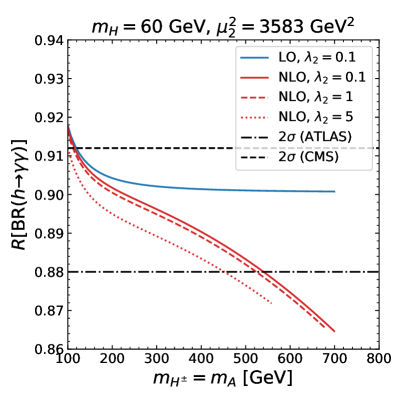
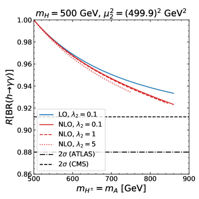
Figure 2: Prediction for $R[\text{BR}(h\to\gamma\gamma)]$ as a function of $m_{H^{\pm}}=m_{A}$. Left: Higgs resonance scenario, defined in Section IV Right: Heavy Higgs scenario, defined in Section IV.

In Fig. 2, we show results for $R[\text{BR}(h\to\gamma\gamma)]$ as a function of $m_{H^{\pm}}=m_{A}$ for the Higgs resonance (left) and the heavy Higgs (right) scenarios. The leading order ($i.e.$ one-loop) result is given by the blue curve, while the red curves correspond to the NLO ($i.e.$ two-loop) results for different values of the inert quartic coupling $\lambda_{2}$. The black lines indicate the expected 95% CL bounds on the ratio $R[\text{BR}(h\to\gamma\gamma)]$ at HL-LHC [33]: the dot-dashed line corresponds to the more conservative limit from ATLAS, while the dashed line is the stronger limit from CMS (which has a better detector for photons). We note that the corresponding current LHC bounds [88, 29, 30] correspond to $R[\text{BR}(h\to\gamma\gamma)]=0.8$ and are outside the plots. Turning first to the LO results, we can observe that the BSM deviation approaches a plateau as $m_{H^{\pm}}$ increases (for the heavy Higgs scenario, this plateau is however not reached due to the limit from perturbative unitarity). This behavior can be explained by the compensation between the charged-Higgs mass dependence in the coupling $\lambda_{3}\propto(m_{H^{\pm}}^{2}-\mu_{2}^{2})$ and in the loop function for the charged Higgs loop at LO — see for instance equations (A.34)-(A.35) in Ref. [10]. At two loops, this situation is drastically modified, and in both scenarios the two-loop corrections to $\Gamma(h\to\gamma\gamma)$ continue growing with $m_{H^{\pm}}$. On the one hand, the parametric dependence of the two-loop corrections — $c.f.$ Section III — is different, so that these still grow for fixed $\mu_{2}$ and increasing $m_{H^{\pm}}$. On the other hand, several new types of contributions arise at two loops that are not corrections of the LO BSM effects — specifically the ${\mathcal{O}(\lambda_{3}^{2})}$ terms can be understood as a correction of the LO ${\mathcal{O}(\lambda_{3})}$ charged-Higgs loop, while the ${\mathcal{O}((\lambda_{4}+\lambda_{5})^{2})}$ and ${\mathcal{O}(\lambda_{2})}$ terms as well as the external-leg corrections correspond to new classes of effects only entering $\Gamma(h\to\gamma\gamma)$ from two loops. Importantly, we find that the inclusion of two-loop corrections in the di-photon decay width increases the size of the BSM deviation. To be concrete, we can consider the situation in the Higgs resonance scenario for $m_{H^{\pm}}=500$ GeV: we find that the deviation of about $-10\%$ at one loop increases to about $-11.5\%$ for low values of $\lambda_{2}$ ($=0.1$ or $1$) or almost $-12.5\%$ for large $\lambda_{2}=5$. In the heavy Higgs scenario and for $m_{H^{\pm}}=700$ GeV, the BSM deviation in $R[\text{BR}(h\to\gamma\gamma)]$ is $-5\%$ at one loop and grows to between $-5.5\%$ and $-6\%$ at two loops (for the values of $\lambda_{2}$ considered here). For the Higgs resonance scenario, the two-loop corrections can even allow the deviation to become larger than the expected precision at the HL-LHC, no matter which bound (stronger from CMS or more conservative from ATLAS) is considered — specifically the bound from ATLAS is exceeded for $m_{H^{\pm}}\gtrsim 550$ GeV (for small values of $\lambda_{2}=0.1$ or $1$) or $m_{H^{\pm}}\gtrsim 450$ GeV (for larger $\lambda_{2}=5$). In other words, the inclusion of two-loop corrections is necessary to properly interpret the observation or non-observation of deviations in $R[\text{BR}(h\to\gamma\gamma)]$ in terms of the parameter space of the IDM. Even in the case in which the expected CMS limits can be achieved, the inclusion of the NLO corrections is paramount to correctly interpret a possible deviation in $R[\text{BR}(h\to\gamma\gamma)]$.

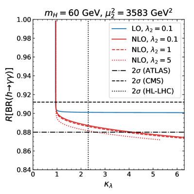
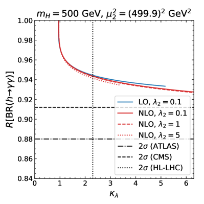
Figure 3: Correlation between $\kappa_{\lambda}$ and $R[\text{BR}(h\to\gamma\gamma)]$ at one loop (blue) and two loops (red). Left: DM-inspired Higgs resonance scenario. Right: Heavy Higgs scenario.

Correlations between BSM deviations in various couplings of the 125-GeV Higgs boson can play a crucial role in identifying, or “fingerprinting,” the nature of the underlying BSM physics at the origin of the deviations — this was for instance pointed out in Ref. [19]. However, in this context, it is also important to assess how higher-order corrections to the different couplings can modify the correlations found at LO. Therefore, we illustrate in Fig. 3 the interplay between $R[\text{BR}(h\to\gamma\gamma)]$ and $\kappa_{\lambda}$ and how it is modified when going from LO to NLO in the calculation of these two quantities. $\kappa_{\lambda}$ denotes here the coupling modifier for the trilinear Higgs coupling, defined as $\kappa_{\lambda}\equiv\lambda_{hhh}^{\text{IDM}}/(\lambda_{hhh}^{\text{SM}})^{(0)}$, with $\lambda_{hhh}^{\text{IDM}}$ the trilinear Higgs coupling calculated at one and two loops in the IDM and with $(\lambda_{hhh}^{\text{SM}})^{(0)}$ the tree-level prediction for this coupling in the SM. As in the previous figure, we consider both benchmark scenarios (Higgs resonance on the left and heavy Higgs on the right), and the blue and red curves correspond to one- and two-loop results respectively. Each of these lines is obtained by varying $m_{H^{\pm}}=m_{A}$ in the ranges given in Sections IV and IV. For the values of $\kappa_{\lambda}$ shown in Fig. 3, we perform a full one-loop calculation of $\kappa_{\lambda}$ with the public tool anyH3 [91], which we complement at the two-loop level by employing results from Refs. [25, 26]. These results were derived for the Higgs resonance scenario ($i.e.$ they include only the dependence on $m_{A}$, $m_{H^{\pm}}$ and $\lambda_{2}$), and we have moreover extended them for use in the heavy Higgs scenario by including also the full dependence on $m_{H}$ and $\mu_{2}$ in $\lambda_{hhh}$ — we provide the new expressions in the appendix. Black lines indicate the expected limits at the HL-LHC [33] for $R[\text{BR}(h\to\gamma\gamma)]$ (the dot-dashed line corresponds to the ATLAS limit, and the dashed line to the CMS one) and $\kappa_{\lambda}$ (dotted line, obtained from a combination of ATLAS and CMS expected bounds). The range of values for $\kappa_{\lambda}$ shown on the horizontal axis is stopped at 6.3, which is the current upper bound on this effective coupling [89, 29, 30, 90].

For the lower end of the mass ranges in both scenarios ($i.e.$ in the upper left corner of the plots), the BSM effects in $R[\text{BR}(h\to\gamma\gamma)]$ grow faster, in relative values, than those in $\kappa_{\lambda}$. However, the size of the deviations in the latter are of course much larger, with effects of several hundred percent being possible — as observed also in $e.g.$ Refs. [17, 25, 26, 28]. In the heavy Higgs scenario (right plot), the two-loop corrections to $R[\text{BR}(h\to\gamma\gamma)]$ are not significant enough to modify the correlation with $\kappa_{\lambda}$ drastically. Moreover, as seen already in Fig. 2, even at the HL-LHC, it seems difficult to access BSM deviations in $R[\text{BR}(h\to\gamma\gamma)]$ for this scenario, and $\kappa_{\lambda}$ appears to offer better prospects of probing the IDM with heavy inert scalars — $\kappa_{\lambda}$ already excludes masses above about 820 GeV (similarly to what was found in Ref. [28]), and at the HL-LHC the mass range above 700 GeV could be probed. On the other hand, the situation is once again more interesting for the Higgs resonance scenario (left plot). The two-loop corrections to $R[\text{BR}(h\to\gamma\gamma)]$ are here sizeable, and the shape of the $R[\text{BR}(h\to\gamma\gamma)]$ vs $\kappa_{\lambda}$ curves are noticeably modified by the inclusion of two-loop corrections and it is clearly necessary to include all known higher-order BSM corrections to both quantities to reliably investigate their interplay. Furthermore, while at present one does not expect to see any deviation in $R[\text{BR}(h\to\gamma\gamma)]$ and in $\kappa_{\lambda}$ only the upper end of the mass range is accessible, almost the entire mass range in this scenario — $i.e.$ $m_{H^{\pm}}\gtrsim 120$ GeV — can be probed at the HL-LHC (considering the expected bound from CMS), and $R[\text{BR}(h\to\gamma\gamma)]$ appears to be more sensitive $\kappa_{\lambda}$ for lower masses. Even in the conservative case in which only the looser limit from ATLAS is achieved, masses above $m_{H^{\pm}}\gtrsim 400-500\text{ GeV}$ would still be accessible at the HL-LHC via $\kappa_{\lambda}$ and $R[\text{BR}(h\to\gamma\gamma)]$. Finally, we note that combined measurements of $R[\text{BR}(h\to\gamma\gamma)]$ and $\kappa_{\lambda}$ offer the interesting possibility of obtaining information about the inert quartic coupling $\lambda_{2}$ that is otherwise very difficult to probe.

V Discussion and conclusion

We have performed in this paper the first calculation of leading two-loop (NLO) BSM corrections to the decay of a Higgs boson into two photons in the IDM. In line with our goal of assessing the size of the dominant two-loop effects, we have considered only contributions involving inert scalars, and we have neglected the dependence on light scalar masses. These assumptions allowed us to use a Higgs LET to obtain compact analytic expressions for the leading two-loop corrections to $\Gamma(h\to\gamma\gamma)$. Additionally, we employed a full on-shell renormalization scheme, including for the BSM mass parameter $\mu_{2}$, for which we found that the “OS” prescription devised for computations of the trilinear Higgs coupling in Refs. [25, 26] also applies in the present case, and ensures the desired renormalization-scale independence as well as apparent and proper decoupling of the BSM contributions.

We have investigated the numerical impact of our new results for two benchmark scenarios inspired by DM phenomenology — the Higgs resonance scenario with $H$ as a light DM candidate and the heavy Higgs scenario where all inert scalars, including the DM candidate $H$, are heavy. We furthermore imposed for these scenarios state-of-the-art theoretical constraints (in particular perturbative unitarity and vacuum stability) as well as experimental limits from collider and DM searches.

We have shown that the two-loop corrections to $\Gamma(h\to\gamma\gamma)$ can become significant in the presence of large mass splittings (in our case between $m_{H}\sim\mu_{2}$ and $m_{H^{\pm}}=m_{A}$). While one would not expect to see deviations in $R[\text{BR}(h\to\gamma\gamma)]$ arising from the inert scalars with the present LHC limits, deviations could appear with data from the HL-LHC. In this regard, the Higgs resonance scenario is especially promising and, in this type of scenario, the heavy mass range for $A$ and $H^{\pm}$ could be ruled out in the near future (even if one only considers the conservative expected limit from ATLAS). It is particularly important to emphasize here that this result requires the inclusion of two-loop BSM corrections to the di-photon decay width, and a leading-order calculation does not suffice to interpret HL-LHC limits on $R[\text{BR}(h\to\gamma\gamma)]$ in terms of the IDM parameter space reliably. On the other hand, the heavy Higgs scenario would remain out of reach of measurements of the $h\to\gamma\gamma$ decay at the HL-LHC. Prospects are of course better at possible lepton colliders, with (sub)percent level constraints achievable at an electron-positron machine like the ILC — see for instance Ref. [92]. Investigations of the IDM via its effects on Higgs properties should also be considered in complementarity with direct searches for inert scalars at current and future colliders (see $e.g.$ Ref. [44]). Direct collider searches will probe the lower ranges of masses, but it is interesting to note that they will not rule out large deviations in Higgs couplings (as these occur for larger masses of the BSM scalars). Meanwhile, probes via invisible decays of the 125-GeV Higgs boson or via DM direct detection, typically do not significantly constrain scenarios leading to large deviations in $R[\text{BR}(h\to\gamma\gamma)]$ (or in $\kappa_{\lambda}$), as illustrated by the specific cases considered in this work. Our work strengthens the motivation to compute Higgs properties such as its decay width to two photons beyond leading order, in order to reduce theoretical uncertainties and allow reliable comparisons between theoretical predictions and experimental results.

Further details about our calculations and their phenomenological applications will be provided in future work.

Note added —

Towards the completion of this work, we became aware of a very recent similar calculation of $\Gamma(h\to\gamma\gamma)$ in a different model (the aligned Two-Higgs-Doublet Model) in Ref. [93]. Our results are compatible with those found in this paper.

Appendix A Leading two-loop corrections to $\lambda_{hhh}$ in the IDM

We provide in this appendix expressions for the leading two-loop corrections to the trilinear Higgs coupling $\lambda_{hhh}$ in the IDM — extending the results of Refs. [25, 26]. As in these references, we obtain the new expressions using the effective-potential approximation, and with a full on-shell renormalization scheme.

For convenience, we decompose the two-loop corrections to $\lambda_{hhh}$ — which we denote $\delta^{(2)}\lambda_{hhh}$ — in three pieces, as

$$\delta^{(2)}\lambda_{hhh}= \ \delta^{(2)}\lambda_{hhh}\big{|}_{SS}+\delta^{(2)}\lambda_{hhh}\big{|}_{SSS}$$

$$+\delta^{(2)}\lambda_{hhh}\big{|}_{\text{ext-leg+VEV}}\,.$$ (25)

In this equation, the three pieces correspond respectively to eight-shaped and sunrise diagrams in the effective potential (see $e.g.$ Ref. [60] for a description of two-loop contributions to the effective potential) and to one-loop-squared contributions from external-leg corrections and VEV renormalization. We find

$$\delta^{(2)}\lambda_{hhh}\big{|}_{SS}=\frac{6\lambda_{2}}{(16\pi^{2})^{2}v^{3}} \Bigg{[}3\left(m_{H}^{4}-6m_{H}^{2}\mu_{2}^{2}-\frac{2\mu_{2}^{6}}{m_{H}^{2}}\right)+3\left(m_{A}^{4}-6m_{A}^{2}\mu_{2}^{2}-\frac{2\mu_{2}^{6}}{m_{A}^{2}}\right)+4\left(2m_{H^{\pm}}^{4}-9m_{H^{\pm}}^{2}\mu_{2}^{2}-\frac{3\mu_{2}^{6}}{m_{H^{\pm}}^{2}}\right)$$

$$+2m_{H}^{2}m_{A}^{2}+4m_{H}^{2}m_{H^{\pm}}^{2}+4m_{A}^{2}m_{H^{\pm}}^{2}+\mu_{2}^{4}\left(\frac{m_{H}^{4}+m_{A}^{4}}{m_{H}^{2}m_{A}^{2}}+\frac{2(m_{H}^{4}+m_{H^{\pm}}^{4})}{m_{H}^{2}m_{H^{\pm}}^{2}}+\frac{2(m_{A}^{4}+m_{H^{\pm}}^{4})}{m_{A}^{2}m_{H^{\pm}}^{2}}\right)$$

$$+62\mu_{2}^{4}-\frac{2\mu_{2}^{2}}{m_{H}^{2}}\left((m_{H}^{2}-\mu_{2}^{2})^{2}\log\frac{m_{H}^{2}}{m_{H^{\pm}}^{2}}-2m_{H}^{2}\mu_{2}^{2}\log\frac{m_{A}^{2}}{m_{H^{\pm}}^{2}}\right)$$

$$-\frac{2\mu_{2}^{2}}{m_{A}^{2}}\left((m_{A}^{2}-\mu_{2}^{2})^{2}\log\frac{m_{A}^{2}}{m_{H^{\pm}}^{2}}-2m_{A}^{2}\mu_{2}^{2}\log\frac{m_{H}^{2}}{m_{H^{\pm}}^{2}}\right)\Bigg{]}\,.$$ (26)

$$\delta^{(2)}\lambda_{hhh}\big{|}_{SSS}=\frac{4}{(16\pi^{2})^{2}v^{5}} \Bigg{\{}12m_{H}^{6}\left(1-\frac{\mu_{2}^{2}}{m_{H}^{2}}\right)^{4}+12m_{A}^{6}\left(1-\frac{\mu_{2}^{2}}{m_{A}^{2}}\right)^{4}+24m_{H^{\pm}}^{6}\left(1-\frac{\mu_{2}^{2}}{m_{H^{\pm}}^{2}}\right)^{4}$$ (27)

$$+(m_{H}^{2}-m_{A}^{2})^{2}\bigg{[}\mu_{2}^{6}\left(\frac{1}{m_{H}^{4}}+\frac{1}{m_{A}^{4}}\right)+3(m_{H}^{2}+m_{A}^{2})$$

$$\hskip 85.35826pt+\frac{\mu_{2}^{2}}{m_{H}^{2}m_{A}^{2}}\bigg{(}3\mu_{2}^{2}(m_{H}^{2}+m_{A}^{2})-12m_{H}^{2}m_{A}^{2}-2\mu_{2}^{4}\bigg{)}\bigg{]}$$

$$+(m_{H}^{2}-m_{A}^{2})^{3}\mu_{2}^{2}\bigg{[}\left(\frac{3}{m_{H}^{2}}-\frac{\mu_{2}^{4}}{m_{H}^{6}}\right)\log\left(1-\frac{m_{H}^{2}}{m_{A}^{2}}\right)-\left(\frac{3}{m_{A}^{2}}-\frac{\mu_{2}^{4}}{m_{A}^{6}}\right)\log\left(\frac{m_{A}^{2}}{m_{H}^{2}}-1\right)\bigg{]}$$

$$+2(m_{H}^{2}-m_{H^{\pm}}^{2})^{2}\bigg{[}\mu_{2}^{6}\left(\frac{1}{m_{H}^{4}}+\frac{1}{m_{H^{\pm}}^{4}}\right)+3(m_{H}^{2}+m_{H^{\pm}}^{2})$$

$$\hskip 85.35826pt+\frac{\mu_{2}^{2}}{m_{H}^{2}m_{H^{\pm}}^{2}}\bigg{(}3\mu_{2}^{2}(m_{H}^{2}+m_{H^{\pm}}^{2})-12m_{H}^{2}m_{H^{\pm}}^{2}-2\mu_{2}^{4}\bigg{)}\bigg{]}$$

$$+2(m_{H}^{2}-m_{H^{\pm}}^{2})^{3}\bigg{[}\left(\frac{3\mu_{2}^{2}}{m_{H}^{2}}-\frac{\mu_{2}^{6}}{m_{H}^{6}}\right)\log\left(1-\frac{m_{H}^{2}}{m_{H^{\pm}}^{2}}\right)-\left(\frac{3\mu_{2}^{2}}{m_{H^{\pm}}^{2}}-\frac{\mu_{2}^{6}}{m_{H^{\pm}}^{6}}\right)\log\left(\frac{m_{H^{\pm}}^{2}}{m_{H}^{2}}-1\right)\bigg{]}$$

$$+2(m_{A}^{2}-m_{H^{\pm}}^{2})^{2}\bigg{[}\mu_{2}^{6}\left(\frac{1}{m_{A}^{4}}+\frac{1}{m_{H^{\pm}}^{4}}\right)+3(m_{A}^{2}+m_{H^{\pm}}^{2})$$

$$\hskip 85.35826pt+\frac{\mu_{2}^{2}}{m_{A}^{2}m_{H^{\pm}}^{2}}\bigg{(}3\mu_{2}^{2}(m_{A}^{2}+m_{H^{\pm}}^{2})-12m_{A}^{2}m_{H^{\pm}}^{2}-2\mu_{2}^{4}\bigg{)}\bigg{]}$$

$$+2(m_{A}^{2}-m_{H^{\pm}}^{2})^{3}\bigg{[}\left(\frac{3\mu_{2}^{2}}{m_{A}^{2}}-\frac{\mu_{2}^{6}}{m_{A}^{6}}\right)\log\left(1-\frac{m_{A}^{2}}{m_{H^{\pm}}^{2}}\right)-\left(\frac{3\mu_{2}^{2}}{m_{H^{\pm}}^{2}}-\frac{\mu_{2}^{6}}{m_{H^{\pm}}^{6}}\right)\log\left(\frac{m_{H^{\pm}}^{2}}{m_{A}^{2}}-1\right)\bigg{]}\Bigg{\}}\,.$$

$$\delta^{(2)}\lambda_{hhh}\big{|}_{\text{ext-leg+VEV}}=\frac{1}{(16\pi^{2})^{2}v^{5}} \Bigg{\{}42m_{t}^{2}\left[m_{H}^{4}\left(1-\frac{\mu_{2}^{2}}{m_{H}^{2}}\right)^{3}+m_{A}^{4}\left(1-\frac{\mu_{2}^{2}}{m_{A}^{2}}\right)^{3}+2m_{H^{\pm}}^{4}\left(1-\frac{\mu_{2}^{2}}{m_{H^{\pm}}^{2}}\right)^{3}\right]$$

$$+24m_{t}^{4}\left[m_{H}^{2}\left(1-\frac{\mu_{2}^{2}}{m_{H}^{2}}\right)^{2}+m_{A}^{2}\left(1-\frac{\mu_{2}^{2}}{m_{A}^{2}}\right)^{2}+2m_{H^{\pm}}^{2}\left(1-\frac{\mu_{2}^{2}}{m_{H^{\pm}}^{2}}\right)^{2}\right]$$

$$-2\left[m_{H}^{4}\left(1-\frac{\mu_{2}^{2}}{m_{H}^{2}}\right)^{3}+m_{A}^{4}\left(1-\frac{\mu_{2}^{2}}{m_{A}^{2}}\right)^{3}+2m_{H^{\pm}}^{4}\left(1-\frac{\mu_{2}^{2}}{m_{H^{\pm}}^{2}}\right)^{3}\right]$$

$$\hskip 28.45274pt\times\left[m_{H}^{2}\left(1-\frac{\mu_{2}^{2}}{m_{H}^{2}}\right)^{2}+m_{A}^{2}\left(1-\frac{\mu_{2}^{2}}{m_{A}^{2}}\right)^{2}+2m_{H^{\pm}}^{2}\left(1-\frac{\mu_{2}^{2}}{m_{H^{\pm}}^{2}}\right)^{2}\right]\Bigg{\}}\,.$$ (28)

These expressions are manifestly independent of the renormalization scale, as expected from our choice of renormalization prescription. Moreover, we have verified: (i) that these BSM effects decouple properly in the limit $\mu_{2}\to\infty$, and (ii) that in the limit $\mu_{2},m_{H}\to 0$ we recover equation (V.22) of Ref. [26]. Finally, we note that the expression for $\delta^{(2)}\lambda_{hhh}\big{|}_{SSS}$ is provided here for the mass hierarchy $m_{H}<m_{A}<m_{H^{\pm}}$, but it can be adapted for any desired hierarchy by selecting the appropriate branch of the logarithms.

References

- Ade et al. [2016] P. A. R. Ade et al. (Planck), Planck 2015 results. XIII. Cosmological parameters, Astron. Astrophys. 594, A13 (2016), arXiv:1502.01589 [astro-ph.CO] .
- Deshpande and Ma [1978] N. G. Deshpande and E. Ma, Pattern of Symmetry Breaking with Two Higgs Doublets, Phys. Rev. D 18, 2574 (1978).
- Barbieri et al. [2006] R. Barbieri, L. J. Hall, and V. S. Rychkov, Improved naturalness with a heavy Higgs: An Alternative road to LHC physics, Phys. Rev. D 74, 015007 (2006), arXiv:hep-ph/0603188 .
- Aalbers et al. [2022] J. Aalbers et al. (LZ), First Dark Matter Search Results from the LUX-ZEPLIN (LZ) Experiment, (2022), arXiv:2207.03764 [hep-ex] .
- Aprile et al. [2023] E. Aprile et al. (XENON), First Dark Matter Search with Nuclear Recoils from the XENONnT Experiment, (2023), arXiv:2303.14729 [hep-ex] .
- Pierce and Thaler [2007] A. Pierce and J. Thaler, Natural Dark Matter from an Unnatural Higgs Boson and New Colored Particles at the TeV Scale, JHEP 08, 026, arXiv:hep-ph/0703056 .
- Lundstrom et al. [2009] E. Lundstrom, M. Gustafsson, and J. Edsjo, The Inert Doublet Model and LEP II Limits, Phys. Rev. D 79, 035013 (2009), arXiv:0810.3924 [hep-ph] .
- Workman et al. [2022] R. L. Workman et al. (Particle Data Group), Review of Particle Physics, PTEP 2022, 083C01 (2022).
- Arhrib et al. [2015] A. Arhrib, R. Benbrik, J. El Falaki, and A. Jueid, Radiative corrections to the Triple Higgs Coupling in the Inert Higgs Doublet Model, JHEP 12, 007, arXiv:1507.03630 [hep-ph] .
- Kanemura et al. [2016a] S. Kanemura, M. Kikuchi, and K. Sakurai, Testing the dark matter scenario in the inert doublet model by future precision measurements of the Higgs boson couplings, Phys. Rev. D94, 115011 (2016a), arXiv:1605.08520 [hep-ph] .
- Kanemura et al. [2019] S. Kanemura, M. Kikuchi, K. Mawatari, K. Sakurai, and K. Yagyu, Full next-to-leading-order calculations of Higgs boson decay rates in models with non-minimal scalar sectors, Nucl. Phys. B 949, 114791 (2019), arXiv:1906.10070 [hep-ph] .
- Apo [2017] High-Luminosity Large Hadron Collider (HL-LHC): Technical Design Report V. 0.1 4/2017, 10.23731/CYRM-2017-004 (2017).
- ILC [2013] The International Linear Collider Technical Design Report - Volume 2: Physics, (2013), arXiv:1306.6352 [hep-ph] .
- Abada et al. [2019] A. Abada et al. (FCC), FCC-ee: The Lepton Collider: Future Circular Collider Conceptual Design Report Volume 2, Eur. Phys. J. ST 228, 261 (2019).
- Dong et al. [2018] M. Dong et al. (CEPC Study Group), CEPC Conceptual Design Report: Volume 2 - Physics & Detector, (2018), arXiv:1811.10545 [hep-ex] .
- Kanemura et al. [2003] S. Kanemura, S. Kiyoura, Y. Okada, E. Senaha, and C. P. Yuan, New physics effect on the Higgs selfcoupling, Phys. Lett. B558, 157 (2003), arXiv:hep-ph/0211308 [hep-ph] .
- Kanemura et al. [2004] S. Kanemura, Y. Okada, E. Senaha, and C. P. Yuan, Higgs coupling constants as a probe of new physics, Phys. Rev. D70, 115002 (2004), arXiv:hep-ph/0408364 [hep-ph] .
- Aoki et al. [2013] M. Aoki, S. Kanemura, M. Kikuchi, and K. Yagyu, Radiative corrections to the Higgs boson couplings in the triplet model, Phys. Rev. D87, 015012 (2013), arXiv:1211.6029 [hep-ph] .
- Kanemura et al. [2015] S. Kanemura, M. Kikuchi, and K. Yagyu, Fingerprinting the extended Higgs sector using one-loop corrected Higgs boson couplings and future precision measurements, Nucl. Phys. B896, 80 (2015), arXiv:1502.07716 [hep-ph] .
- Kanemura et al. [2016b] S. Kanemura, M. Kikuchi, and K. Yagyu, Radiative corrections to the Higgs boson couplings in the model with an additional real singlet scalar field, Nucl. Phys. B907, 286 (2016b), arXiv:1511.06211 [hep-ph] .
- He and Zhu [2017] S.-P. He and S.-h. Zhu, One-Loop Radiative Correction to the Triple Higgs Coupling in the Higgs Singlet Model, Phys. Lett. B764, 31 (2017), arXiv:1607.04497 [hep-ph] .
- Kanemura et al. [2017a] S. Kanemura, M. Kikuchi, and K. Yagyu, One-loop corrections to the Higgs self-couplings in the singlet extension, Nucl. Phys. B917, 154 (2017a), arXiv:1608.01582 [hep-ph] .
- Kanemura et al. [2017b] S. Kanemura, M. Kikuchi, K. Sakurai, and K. Yagyu, Gauge invariant one-loop corrections to Higgs boson couplings in non-minimal Higgs models, Phys. Rev. D96, 035014 (2017b), arXiv:1705.05399 [hep-ph] .
- Senaha [2019] E. Senaha, Radiative Corrections to Triple Higgs Coupling and Electroweak Phase Transition: Beyond One-loop Analysis, Phys. Rev. D100, 055034 (2019), arXiv:1811.00336 [hep-ph] .
- Braathen and Kanemura [2019] J. Braathen and S. Kanemura, On two-loop corrections to the Higgs trilinear coupling in models with extended scalar sectors, Phys. Lett. B 796, 38 (2019), arXiv:1903.05417 [hep-ph] .
- Braathen and Kanemura [2020] J. Braathen and S. Kanemura, Leading two-loop corrections to the Higgs boson self-couplings in models with extended scalar sectors, Eur. Phys. J. C 80, 227 (2020), arXiv:1911.11507 [hep-ph] .
- Braathen et al. [2021] J. Braathen, S. Kanemura, and M. Shimoda, Two-loop analysis of classically scale-invariant models with extended Higgs sectors, JHEP 03, 297, arXiv:2011.07580 [hep-ph] .
- Bahl et al. [2022a] H. Bahl, J. Braathen, and G. Weiglein, New Constraints on Extended Higgs Sectors from the Trilinear Higgs Coupling, Phys. Rev. Lett. 129, 231802 (2022a), arXiv:2202.03453 [hep-ph] .
- ATL [2022a] A detailed map of Higgs boson interactions by the ATLAS experiment ten years after the discovery, Nature 607, 52 (2022a), [Erratum: Nature 612, E24 (2022)], arXiv:2207.00092 [hep-ex] .
- Tumasyan et al. [2022] A. Tumasyan et al. (CMS), A portrait of the Higgs boson by the CMS experiment ten years after the discovery, Nature 607, 60 (2022), arXiv:2207.00043 [hep-ex] .
- Arhrib et al. [2012] A. Arhrib, R. Benbrik, and N. Gaur, in Inert Higgs Doublet Model, Phys. Rev. D 85, 095021 (2012), arXiv:1201.2644 [hep-ph] .
- Swiezewska and Krawczyk [2013] B. Swiezewska and M. Krawczyk, Diphoton rate in the inert doublet model with a 125 GeV Higgs boson, Phys. Rev. D 88, 035019 (2013), arXiv:1212.4100 [hep-ph] .
- Cepeda et al. [2019] M. Cepeda et al. (Physics of the HL-LHC Working Group), Higgs Physics at the HL-LHC and HE-LHC, arXiv:1902.00134 [hep-ph] (2019).
- Shifman et al. [1979] M. A. Shifman, A. I. Vainshtein, M. B. Voloshin, and V. I. Zakharov, Low-Energy Theorems for Higgs Boson Couplings to Photons, Sov. J. Nucl. Phys. 30, 711 (1979).
- Kniehl and Spira [1995] B. A. Kniehl and M. Spira, Low-energy theorems in Higgs physics, Z. Phys. C 69, 77 (1995), arXiv:hep-ph/9505225 .
- Hessenberger and Hollik [2017] S. Hessenberger and W. Hollik, Two-loop corrections to the parameter in Two-Higgs-Doublet Models, Eur. Phys. J. C 77, 178 (2017), arXiv:1607.04610 [hep-ph] .
- Kanemura et al. [1999] S. Kanemura, T. Kasai, and Y. Okada, Mass bounds of the lightest CP even Higgs boson in the two Higgs doublet model, Phys. Lett. B 471, 182 (1999), arXiv:hep-ph/9903289 .
- Kanemura et al. [1993] S. Kanemura, T. Kubota, and E. Takasugi, Lee-Quigg-Thacker bounds for Higgs boson masses in a two doublet model, Phys. Lett. B 313, 155 (1993), arXiv:hep-ph/9303263 .
- Akeroyd et al. [2000] A. G. Akeroyd, A. Arhrib, and E.-M. Naimi, Note on tree level unitarity in the general two Higgs doublet model, Phys. Lett. B 490, 119 (2000), arXiv:hep-ph/0006035 .
- Ginzburg et al. [2010] I. F. Ginzburg, K. A. Kanishev, M. Krawczyk, and D. Sokolowska, Evolution of Universe to the present inert phase, Phys. Rev. D 82, 123533 (2010), arXiv:1009.4593 [hep-ph] .
- Belanger et al. [2015] G. Belanger, B. Dumont, A. Goudelis, B. Herrmann, S. Kraml, and D. Sengupta, Dilepton constraints in the Inert Doublet Model from Run 1 of the LHC, Phys. Rev. D 91, 115011 (2015), arXiv:1503.07367 [hep-ph] .
- Ilnicka et al. [2016] A. Ilnicka, M. Krawczyk, and T. Robens, Inert Doublet Model in light of LHC Run I and astrophysical data, Phys. Rev. D 93, 055026 (2016), arXiv:1508.01671 [hep-ph] .
- Belyaev et al. [2019] A. Belyaev, T. R. Fernandez Perez Tomei, P. G. Mercadante, C. S. Moon, S. Moretti, S. F. Novaes, L. Panizzi, F. Rojas, and M. Thomas, Advancing LHC probes of dark matter from the inert two-Higgs-doublet model with the monojet signal, Phys. Rev. D 99, 015011 (2019), arXiv:1809.00933 [hep-ph] .
- Kalinowski et al. [2021] J. Kalinowski, T. Robens, D. Sokolowska, and A. F. Zarnecki, IDM Benchmarks for the LHC and Future Colliders, Symmetry 13, 991 (2021), arXiv:2012.14818 [hep-ph] .
- Peskin and Takeuchi [1992] M. E. Peskin and T. Takeuchi, Estimation of oblique electroweak corrections, Phys. Rev. D 46, 381 (1992).
- Belyaev et al. [2018] A. Belyaev, G. Cacciapaglia, I. P. Ivanov, F. Rojas-Abatte, and M. Thomas, Anatomy of the Inert Two Higgs Doublet Model in the light of the LHC and non-LHC Dark Matter Searches, Phys. Rev. D 97, 035011 (2018), arXiv:1612.00511 [hep-ph] .
- Hessenberger and Hollik [2022] S. Hessenberger and W. Hollik, Two-loop improved predictions for and in Two-Higgs-Doublet models, Eur. Phys. J. C 82, 970 (2022), arXiv:2207.03845 [hep-ph] .
- Bélanger et al. [2018] G. Bélanger, F. Boudjema, A. Goudelis, A. Pukhov, and B. Zaldivar, micrOMEGAs5.0 : Freeze-in, Comput. Phys. Commun. 231, 173 (2018), arXiv:1801.03509 [hep-ph] .
- Slavich et al. [2021] P. Slavich et al., Higgs-mass predictions in the MSSM and beyond, Eur. Phys. J. C 81, 450 (2021), arXiv:2012.15629 [hep-ph] .
- Kublbeck et al. [1990] J. Kublbeck, M. Bohm, and A. Denner, Feyn Arts: Computer Algebraic Generation of Feynman Graphs and Amplitudes, Comput. Phys. Commun. 60, 165 (1990).
- Hahn [2001] T. Hahn, Generating Feynman diagrams and amplitudes with FeynArts 3, Comput. Phys. Commun. 140, 418 (2001), arXiv:hep-ph/0012260 .
- Staub [2010] F. Staub, From Superpotential to Model Files for FeynArts and CalcHep/CompHep, Comput. Phys. Commun. 181, 1077 (2010), arXiv:0909.2863 [hep-ph] .
- Staub [2011] F. Staub, Automatic Calculation of supersymmetric Renormalization Group Equations and Self Energies, Comput. Phys. Commun. 182, 808 (2011), arXiv:1002.0840 [hep-ph] .
- Staub [2013] F. Staub, SARAH 3.2: Dirac Gauginos, UFO output, and more, Comput. Phys. Commun. 184, 1792 (2013), arXiv:1207.0906 [hep-ph] .
- Staub [2014] F. Staub, SARAH 4 : A tool for (not only SUSY) model builders, Comput. Phys. Commun. 185, 1773 (2014), arXiv:1309.7223 [hep-ph] .
- Mertig et al. [1991] R. Mertig, M. Bohm, and A. Denner, FEYN CALC: Computer algebraic calculation of Feynman amplitudes, Comput. Phys. Commun. 64, 345 (1991).
- Shtabovenko et al. [2016] V. Shtabovenko, R. Mertig, and F. Orellana, New Developments in FeynCalc 9.0, Comput. Phys. Commun. 207, 432 (2016), arXiv:1601.01167 [hep-ph] .
- Shtabovenko et al. [2020] V. Shtabovenko, R. Mertig, and F. Orellana, FeynCalc 9.3: New features and improvements, Comput. Phys. Commun. 256, 107478 (2020), arXiv:2001.04407 [hep-ph] .
- Mertig and Scharf [1998] R. Mertig and R. Scharf, TARCER: A Mathematica program for the reduction of two loop propagator integrals, Comput. Phys. Commun. 111, 265 (1998), arXiv:hep-ph/9801383 .
- Martin [2002] S. P. Martin, Two Loop Effective Potential for a General Renormalizable Theory and Softly Broken Supersymmetry, Phys. Rev. D 65, 116003 (2002), arXiv:hep-ph/0111209 .
- Martin [2003] S. P. Martin, Evaluation of two loop selfenergy basis integrals using differential equations, Phys. Rev. D 68, 075002 (2003), arXiv:hep-ph/0307101 .
- Braathen and Goodsell [2016] J. Braathen and M. D. Goodsell, Avoiding the Goldstone Boson Catastrophe in general renormalisable field theories at two loops, JHEP 12, 056, arXiv:1609.06977 [hep-ph] .
- Bahl et al. [2022b] H. Bahl, J. Braathen, and G. Weiglein, External leg corrections as an origin of large logarithms, JHEP 02, 159, arXiv:2112.11419 [hep-ph] .
- Martin and Robertson [2006] S. P. Martin and D. G. Robertson, TSIL: A Program for the calculation of two-loop self-energy integrals, Comput. Phys. Commun. 174, 133 (2006), arXiv:hep-ph/0501132 .
- Elias-Miro et al. [2014] J. Elias-Miro, J. R. Espinosa, and T. Konstandin, Taming Infrared Divergences in the Effective Potential, JHEP 08, 034, arXiv:1406.2652 [hep-ph] .
- Martin [2014] S. P. Martin, Taming the Goldstone contributions to the effective potential, Phys. Rev. D 90, 016013 (2014), arXiv:1406.2355 [hep-ph] .
- Kumar and Martin [2016] N. Kumar and S. P. Martin, Resummation of Goldstone boson contributions to the MSSM effective potential, Phys. Rev. D 94, 014013 (2016), arXiv:1605.02059 [hep-ph] .
- Braathen et al. [2017] J. Braathen, M. D. Goodsell, and F. Staub, Supersymmetric and non-supersymmetric models without catastrophic Goldstone bosons, Eur. Phys. J. C 77, 757 (2017), arXiv:1706.05372 [hep-ph] .
- Goodsell and Paßehr [2020] M. D. Goodsell and S. Paßehr, All two-loop scalar self-energies and tadpoles in general renormalisable field theories, Eur. Phys. J. C 80, 417 (2020), arXiv:1910.02094 [hep-ph] .
- Djouadi et al. [1991] A. Djouadi, M. Spira, J. J. van der Bij, and P. M. Zerwas, QCD corrections to gamma gamma decays of Higgs particles in the intermediate mass range, Phys. Lett. B 257, 187 (1991).
- Dawson and Kauffman [1993] S. Dawson and R. P. Kauffman, QCD corrections to H — gamma gamma, Phys. Rev. D 47, 1264 (1993).
- Melnikov and Yakovlev [1993] K. Melnikov and O. I. Yakovlev, Higgs — two photon decay: QCD radiative correction, Phys. Lett. B 312, 179 (1993), arXiv:hep-ph/9302281 .
- Djouadi et al. [1993] A. Djouadi, M. Spira, and P. M. Zerwas, Two photon decay widths of Higgs particles, Phys. Lett. B 311, 255 (1993), arXiv:hep-ph/9305335 .
- Inoue et al. [1994] M. Inoue, R. Najima, T. Oka, and J. Saito, QCD corrections to two photon decay of the Higgs boson and its reverse process, Mod. Phys. Lett. A 9, 1189 (1994).
- Steinhauser [1996] M. Steinhauser, Corrections of O to the decay of an intermediate mass Higgs boson into two photons, in Ringberg Workshop: The Higgs Puzzle - What can We Learn from LEP2, LHC, NLC, and FMC? (1996) pp. 177–185, arXiv:hep-ph/9612395 .
- Fleischer et al. [2004] J. Fleischer, O. V. Tarasov, and V. O. Tarasov, Analytical result for the two loop QCD correction to the decay H — 2 gamma, Phys. Lett. B 584, 294 (2004), arXiv:hep-ph/0401090 .
- Djouadi [2008] A. Djouadi, The Anatomy of electro-weak symmetry breaking. I: The Higgs boson in the standard model, Phys. Rept. 457, 1 (2008), arXiv:hep-ph/0503172 .
- Djouadi et al. [1998] A. Djouadi, P. Gambino, and B. A. Kniehl, Two loop electroweak heavy fermion corrections to Higgs boson production and decay, Nucl. Phys. B 523, 17 (1998), arXiv:hep-ph/9712330 .
- Fugel et al. [2004] F. Fugel, B. A. Kniehl, and M. Steinhauser, Two loop electroweak correction of O(G(F)M(t)**2) to the Higgs-boson decay into photons, Nucl. Phys. B 702, 333 (2004), arXiv:hep-ph/0405232 .
- Aglietti et al. [2004] U. Aglietti, R. Bonciani, G. Degrassi, and A. Vicini, Two loop light fermion contribution to Higgs production and decays, Phys. Lett. B 595, 432 (2004), arXiv:hep-ph/0404071 .
- Degrassi and Maltoni [2005] G. Degrassi and F. Maltoni, Two-loop electroweak corrections to the Higgs-boson decay H — gamma gamma, Nucl. Phys. B 724, 183 (2005), arXiv:hep-ph/0504137 .
- Passarino et al. [2007] G. Passarino, C. Sturm, and S. Uccirati, Complete Two-Loop Corrections to H — gamma gamma, Phys. Lett. B 655, 298 (2007), arXiv:0707.1401 [hep-ph] .
- Actis et al. [2009] S. Actis, G. Passarino, C. Sturm, and S. Uccirati, NNLO Computational Techniques: The Cases H — gamma gamma and H — g g, Nucl. Phys. B 811, 182 (2009), arXiv:0809.3667 [hep-ph] .
- Sirlin [1980] A. Sirlin, Radiative Corrections in the SU(2)-L x U(1) Theory: A Simple Renormalization Framework, Phys. Rev. D 22, 971 (1980).
- Biekötter and Pierre [2022] T. Biekötter and M. Pierre, Higgs-boson visible and invisible constraints on hidden sectors, Eur. Phys. J. C 82, 1026 (2022), arXiv:2208.05505 [hep-ph] .
- Kanemura et al. [2018] S. Kanemura, M. Kikuchi, K. Sakurai, and K. Yagyu, H-COUP: a program for one-loop corrected Higgs boson couplings in non-minimal Higgs sectors, Comput. Phys. Commun. 233, 134 (2018), arXiv:1710.04603 [hep-ph] .
- Kanemura et al. [2020] S. Kanemura, M. Kikuchi, K. Mawatari, K. Sakurai, and K. Yagyu, H-COUP Version 2: a program for one-loop corrected Higgs boson decays in non-minimal Higgs sectors, Comput. Phys. Commun. 257, 107512 (2020), arXiv:1910.12769 [hep-ph] .
- Sirunyan et al. [2021] A. M. Sirunyan et al. (CMS), Measurements of Higgs boson production cross sections and couplings in the diphoton decay channel at = 13 TeV, JHEP 07, 027, arXiv:2103.06956 [hep-ex] .
- Aad et al. [2023] G. Aad et al. (ATLAS), Measurement of the properties of Higgs boson production at = 13 TeV in the channel using 139 fb-1 of collision data with the ATLAS experiment , JHEP 07, 088, arXiv:2207.00348 [hep-ex] .
- ATL [2022b] Constraining the Higgs boson self-coupling from single- and double-Higgs production with the ATLAS detector using collisions at TeV, (2022b).
- Bahl et al. [2023] H. Bahl, J. Braathen, M. Gabelmann, and G. Weiglein, anyH3: precise predictions for the trilinear Higgs coupling in the Standard Model and beyond, (2023), arXiv:2305.03015 [hep-ph] .
- Fujii et al. [2017] K. Fujii et al., Physics Case for the 250 GeV Stage of the International Linear Collider, arXiv:1710.07621 [hep-ex] (2017).
- Degrassi and Slavich [2023] G. Degrassi and P. Slavich, On the two-loop BSM corrections to in the aligned THDM, (2023), arXiv:2307.02476 [hep-ph] .