Insufficient Gibbs Sampling

Abstract

In some applied scenarios, the availability of complete data is restricted, often due to privacy concerns, and only aggregated, robust and inefficient statistics derived from the data are accessible. These robust statistics are not sufficient, but they demonstrate reduced sensitivity to outliers and offer enhanced data protection due to their higher breakdown point. In this article, operating within a parametric framework, we propose a method to sample from the posterior distribution of parameters conditioned on different robust and inefficient statistics: specifically, the pairs (median, MAD) or (median, IQR), or one or more quantiles. Leveraging a Gibbs sampler and the simulation of latent augmented data, our approach facilitates simulation according to the posterior distribution of parameters belonging to specific families of distributions. We demonstrate its applicability on the Gaussian, Cauchy, and translated Weibull families.

1 Introduction

Tukey [18] highlighted the sensitivity of traditional statistical methods to deviations from Gaussian assumptions. This led to theoretical advancements by Huber [11] and Hampel [8], laying the foundation for robust statistical techniques.

Due to data protection laws, the sharing of sensitive personal data is restricted among businesses and scientific institutions. To address this, organizations such as Eurostat and the World Bank often do not release individual-level data $X$, but only robust and insufficient aggregated summary statistics $T(X)$ instead. In other cases, observations may be summarized with robust statistics to reduce the impact of outliers or of model misspecification. This limitation creates a need for statistical methods that can effectively infer parameters from observed robust statistics. In the Bayesian setting, we might impose a parametric distribution $(\mathcal{F}_{\theta})_{\theta\in\Theta}$ on the original observations, and wish to sample from the posterior distribution of $\theta$ given robust statistics. The posterior distribution is typically intractable, making its simulation challenging and an interesting area of research. Previous studies have employed Approximate Bayesian Computation (ABC) with robust summary statistics, such as the median, Median Absolute Deviation (MAD), or Interquartile Range (IQR) [19, 7, 13]. Huang et al [10] argue that for ABC or other simulation-based inference methods, robust summary statistics make the pseudo-posterior robust to model misspecification [5]. While ABC provides an approach to infer posterior distributions when likelihood evaluations are difficult, these methods only enable simulation from an approximation of the posterior distribution and are less satisfactory than a scheme to sample from the exact posterior. Matching quantiles have also been explored in various contexts [15, 14].

We propose here a method to sample from the posterior distribution of $\theta$ given robust statistics $T(X)$ using augmented data simulation on $X$ as in Tanner and Wong [17], from a parametric family $(\mathcal{F}_{\theta})_{\theta\in\Theta}$. This is achieved through a two-step Gibbs sampler based on a decomposition:

$$\pi\left(\theta\mid T(X)\right)\propto\int_{\mathbb{R}^{N}}\pi(\theta,X\mid T(X))dX\propto\int_{\mathbb{R}^{N}}\pi(\theta\mid X)\pi(X\mid T(X),\theta)dX$$

Thus, in each iteration, we first simulate from $X\mid T(X),\theta$ and then simulate from $\theta\mid X$ assuming $X\sim\mathcal{F}_{\theta}$. We discuss in detail the first step, which is the main contribution of this work. The second step can be straightforward when the distribution family admits a conjugate prior (e.g., Gaussian case) or by using a Metropolis-within-Gibbs step in other cases. We consider specific cases where $T$ is a pair of robust location and scale statistics, such as (median, Median Absolute Deviation) and (median, Interquartile Range), as well as cases where $T$ is a collection of empirical quantiles of $X$. Our only assumption on the family of distributions $\mathcal{F}_{\theta}$ is that we can evaluate pointwise the probability density function $f_{\theta}$ and the cumulative density function $F_{\theta}$. In this setting, it is in particular possible to sample from a truncated distribution, either directly or by rejection sampling. The examples we consider are the Gaussian and Cauchy distributions from the location-scale family, and the translated Weibull distribution. However, our strategy can be applied to other continuous distribution families.

The paper is structured as follows: In Section 2, we introduce our method for observing a sequence of quantiles. Then, in Section 3, we address the scenario where only the median and the interquartile range are observed. The most intriguing case of observing the median and the Median Absolute Deviation (MAD) of the sample is discussed in Section 4. Finally, we discuss some compelling numerical results in Section 5.

2 Quantile case

We first present the case where the observed robust statistics are a set of quantiles. This setting has already been considered in the literature, but our approach uses a different method, which we will extend in later sections to more complex sets of robust statistics.

In this section, we consider the case where we observe a vector of $M\in\mathbb{N}^{*}$ quantiles of the data $X$. A collection of probabilities $(p_{j})_{j=1\ldots M}$ is pre-specified, and we observe $T(X)=(q_{j})_{j=1\ldots M}$ where $q_{j}$ is the empirical $p_{j}$ quantile of $X$.

Akinshin [1] also proposed an MCMC method, implemented in STAN (NUTS or HMC versions), to sample from the posterior distribution when only quantiles are observed. However, they treat the observed quantiles as theoretical ones, and thus assume that they observe the collection $\left(F_{\theta}^{(-1)}(p_{j})\right)$. This assumption is reasonable when the sample size $N$ is large. However, observed quantiles are actually calculated differently in most standard software, and this assumption can lead to a bias in the posterior inference of the parameters, especially with small sample sizes $N$. Therefore, in this paper, we adopt a different approach by considering the observed quantiles as empirical quantiles obtained from the widely used quantile estimator $Q(\cdot,p)$, as defined in Hyndman and Fan [12, Definition 7]. This estimator is commonly implemented in major statistical software: it is for example the default of the quantile() function in R, the default of the Python function numpy.quantile, the default of the Julia function Statistics.quantile!, and the behavior of the PERCENTILE function in Excel. It is given by the following formula:

$$Q(X,p)=(1-g)X_{(i)}+gX_{(i+1)}$$ (1)

where $h=(N-1)p+1$, $i=\lfloor h\rfloor$ (the integer part of $h$), and $g=h-i$ (the fractional part of $h$). We will later note those variables $h_{j},i_{j}$ and $g_{j}$ for the observed $p_{j}$ quantile. Note that other definitions of the empirical quantile function, corresponding to slightly different linear interpolations, were also proposed by Hyndman and Fan [12] and are available in certain software; our approach can easily be adapted to any of these alternative definitions.

We now develop a computational method to simulate a vector $X$ that follows a distribution $\mathcal{F}_{\theta}$ and satisfies the conditions $Q(X,p_{j})=q_{j}$ for $j=1,\dots,J$, where $Q$ is the quantile estimator.

In this scenario, we have complete knowledge of the apportionment of the vector $X$ across $M+1$ intervals. The theoretical apportionment is presented in Figure 1. However, as we consider the empirical quantiles here, these intervals and proportions may slightly vary.

Figure 1: Apportionment of the vector $X$ with observed $p_{j}$ quantiles $q_{j}$. The values above the axis represent the theoretical proportions of observations contained in these intervals.

This knowledge allows us to resample the vector $X$ while preserving the verified conditions $(Q(X,p_{1}),\dots,Q(X,p_{M}))=(q_{1},\dots,q_{M})$. First, we simulate the coordinates of $X$ that determine the observed quantiles $Q(X,p_{1}),\dots,Q(X,p_{M})$. Second, we simulate the remaining coordinates of $X$ using truncated distributions, ensuring that the correct number of coordinates falls within each zone defined by the previously simulated coordinates. We detail the first step of this process; the second is straightforward.

To simulate these coordinates according to the correct distribution, we must first identify the indexes of the order statistics. From the above definition, we have for $j=1,\dots,M$:

• If $g_{j}=0$, we have $Q(X,p_{j})=X_{(i_{j})}$, which we refer to as “deterministic”, and we denote $i_{j}$ as its index.

• If $g_{j}\neq 0$, we have $Q(X,p_{j})=(1-g_{j})X_{(i_{j})}+g_{j}X_{(i_{j}+1)}$, which we say is a linear combination of the order statistics with indexes $i_{j}$ and $i_{j}+1$. In this case, we sample $X_{(i_{j})}$, and then obtain $X_{(i_{j}+1)}$ as a deterministic transformation of $X_{(i_{j})}$ and $q_{j}$.

We denote $J_{D}=\{j\in\{1,\dots,M\}\mid g_{j}=0\}$ and $J_{S}=\{j\in\{1,\dots,M\}\mid g_{j}>0\}$. We have $\{1,\dots,M\}=J_{D}\cup J_{S}$. Thus, the quantiles of interest $Q(X,p_{1}),\dots,Q(X,p_{M})$ are totally determined by the order statistics of indexes in $I=\{i_{j}\mid j=1,\dots,M\}\cup\{i_{j}+1\mid j\in J_{S}\}$.

Remark 1.

For simplicity, we make the assumption (in our presentation and in our code) that $\forall j,p_{j+1}-p_{j}\geq\frac{2}{N+1}$. Under this assumption, each order statistic appears at most once in the set of empirical constraints of the form of Equation 1; in other words, we assume that $\forall j\in J_{S},i_{j}+1<i_{j+1}$. Our method could easily be generalized to lift this assumption.

In the remainder of this section, we describe our MCMC algorithm for this setting. We begin by proposing a method for initializing a vector $X^{0}$ which satisfies the observed quantiles. This initialization step ensures that our resampled data adheres to the desired quantile values. Subsequently, we introduce a method for global resampling of our augmented data using order statistics results and Markov chain simulations. We used the Metropolis-Hastings algorithm with a kernel to facilitate the generation of new samples based on the order statistics.

2.1 Initialization with observed quantiles

Our algorithm requires an initial value of the vector $X^{0}$ which verifies that $\forall j,Q(X^{0},p_{j})=q_{j}$.

First, we initialize the parameter vector $\theta^{0}$ arbitrarily to enable the simulation of our vector. In order to meet the observed quantiles, we set the order statistics that determine the values in the quantiles. For deterministic quantiles ($g_{j}=0$), we directly assign an observation equal to $q_{j}$. For quantiles requiring simulation, we introduce a positive distance parameter $\epsilon_{j}$. Specifically, for all $j$ in $J_{S}$, we set $X_{(i_{j})}=q_{j}-\epsilon_{j}g_{j}$ and $X_{(i_{j}+1)}=q_{j}+\epsilon_{j}(1-g_{j})$, ensuring that $g_{j}X_{(i_{j}+1)}+(1-g_{j})X_{(i_{j})}=q_{j}$. To enhance the efficiency of our initialization, we can normalize $\epsilon_{j}$ to be equal to the variance of $X_{(i_{j})}$ under the assumption that $X$ follows a distribution denoted as $\mathcal{F}_{\theta^{0}}$. Once these observations have been initialized, we can complete the initial vector $X^{0}$ by simulating the remaining observations in the appropriate intervals using a truncated distribution $\mathcal{F}_{\theta^{0}}$.

2.2 Full resampling with observed quantiles

We present a method for conducting complete resampling of our vector $X$ according to the distribution $\mathcal{F}_{\theta}$, while simultaneously preserving the observed quantile values. As mentioned previously, these quantiles are determined by the order statistics of $I$ (where $I$ represents the previously introduced set of coordinates corresponding to the order statistics that determine the quantile values, i.e., $I=\{i_{j}\mid j=1,\dots,M\}\cup\{i_{j}+1\mid j\in J_{S}\}$). Therefore, we need to simulate the order statistics $(X_{(i_{j})})_{j\in J_{S}}$; recall that the $(X_{(i_{j})})_{j\in I\setminus J_{S}}$ are deterministic conditional on the $(X_{(i_{j})})_{j\in J_{S}}$. Our objective is to simulate from the conditional distribution $(X_{(i_{j})})_{j\in J_{S}}\mid Q(X,p_{j})=q_{j}$ for $j=1,\dots,M$. To achieve this, we compute the density of this distribution up to a constant, enabling us to launch a Markov chain that targets this distribution using a Metropolis-Hastings kernel.

We begin by considering the joint density of the order statistics vector $I$. The joint probability density function of $M$ statistics of order $(i_{1},\dots,i_{M})$ from a vector $X$ of size $N$ following a distribution $\mathcal{F}_{\theta}$ with density $f_{\theta}$ and cumulative distribution function (cdf) $F_{\theta}$, is known and can be expressed as shown in Equation 2, which is derived from David and Nagaraja [4]:

$$f(x_{1},\dots,x_{M})=N!\prod_{j=1}^{M}f_{\theta}(x_{j})\prod_{j=0}^{M}\frac{(F_{\theta}(x_{j+1})-F_{\theta}(x_{j}))^{i_{j+1}-i_{j}-1}}{(i_{j+1}-i_{j}-1)!}$$ (2)

where $x_{0}=-\infty$, $x_{M+1}=+\infty$, $i_{0}=0$, and $i_{M+1}=N+1$.

To simulate from the joint distribution of $(X_{(i_{j})})_{j\in J_{S}}$ and $(Q(X,p_{j}))_{j=1,\dots,M}$, we perform a change of variables denoted as $\phi$. This transformation is injective and continuously differentiable, ensuring that the determinant of its Jacobian is nonzero. The transformation is described below by the system on the right:

$$\left\{\begin{aligned} q_{j}&=X_{(i_{j})}&\forall j\in J_{D}\\ q_{j}&=(1-g_{j})X_{(i_{j})}+g_{j}X_{(i_{j}+1)}&\forall j\in J_{S}\end{aligned}\right.\iff\left\{\begin{aligned} X_{(i_{j})}&=q_{j}&\forall j\in J_{D}\\ X_{(i_{j}+1)}&=\frac{q_{j}-X_{(i_{j})}(1-g_{j})}{g_{j}}&\forall j\in J_{S}\end{aligned}\right.$$

Finally, as the observed values $q_{j}$ are fixed, we know that the densities of the joint and conditional distributions are proportional. Hence, we have:

$$\begin{split}&f_{(X_{(i_{j})})_{j\in J_{S}}\mid(Q(X,p_{1}),\dots,Q(X,p_{J}))=(q_{1},\dots,q_{j})}(x_{1},\dots,x_{\lvert J_{S}\rvert})\\ &\propto f_{(X_{(i_{j})})_{k\in J_{S}},(Q(X,p_{1}),\dots,Q(X,p_{j}))=(q_{1},\dots,q_{j})}(x_{1},\dots,x_{\lvert J_{S}\rvert},q_{1},\dots,q_{j})\\ &\propto f_{(i)_{i\in I}}(\phi^{-1}(x_{1},\dots,x_{\lvert J_{S}\rvert},q_{1},\dots,q_{j}))\end{split}$$ (3)

We have now obtained the conditional density, up to a constant, of the order statistics of interest given the observed quantiles. This enables us to simulate data based on our specified conditions. Therefore, we can construct a Markov chain that targets the desired distribution by employing a Metropolis-Hastings acceptance kernel. In our case, we utilize a random walk kernel with a variance that can be empirically adjusted. While it is possible to resample all the order statistics simultaneously using a kernel of size $\mathbb{R}^{\lvert J_{S}\rvert}$, for the purpose of achieving higher acceptance rates, we resample them one by one or in parallel.

To maximize acceptance, we recommend normalizing the variance of the kernel of $X_{(i_{j})}$ by a constant $\tilde{c_{j}}=\text{Var}(X_{(i_{j})})/(1-g_{j})$, assuming that $X\sim\mathcal{F}_{\theta}$. Here, we approximate the variance of the order statistics using the formula presented in Baglivo [2, p. 120]: Var$(X_{(i)})\approx\frac{p_{i}(1-p_{i})}{(N+2)f_{\theta}(Q_{\theta}(p_{i}))^{2}}$, where $N$ is the sample size, $p_{i}=\frac{i}{N-1}$, and $f_{\theta}$ and $Q_{\theta}$ are the density and quantile functions of our distribution. This approximation allows us to handle some cases of order statistics with infinite variance as for the Cauchy distribution.

Implementation results for this case are shown in Section 5.3.

3 Median and IQR case

We now present a computational method to simulate a vector $X$ which follows a distribution $\mathcal{F}_{\theta}$ and verifies the conditions $\text{med}(X)=m$ and $\text{IQR}(X)=i$ where $m\in\mathbb{R}$ and $i>0$. Here, $\text{med}(X)$ is the median of $X$, and $\text{IQR}(X)$ is the interquartile range of $X$. The interquartile range is the difference between the 0.75 quantile, which is the third quartile denoted $Q_{3}$, and the 0.25 quantile, which is the first quartile denoted $Q_{1}$, i.e., $\text{IQR}(X)=Q(X,0.75)-Q(X,0.25)=Q_{3}-Q_{1}$. This scale estimator has a long history in robust statistics, dating back to the early development of robust estimation techniques. Its resistance to outliers, as quantified by its breakdown point of 25%, has made it a fundamental tool in robust statistical analysis. Today, the IQR continues to hold a prominent position in robust statistics due to its properties and its ability to summarize the variability of a dataset in a resistant manner. The IQR, being equal to twice the MAD in the case of a symmetric distribution, not only measures the dispersion of the data but also offers a way to capture the asymmetry of the distribution. This section is thus linked to the previous section with the case $p_{1},p_{2},p_{3}=0.25,0.5,0.75$, except we observe only $q_{2}=m$ (the median) and the difference $q_{3}-q_{1}=i$ with $i>0$. In this scenario, we can isolate four different cases and we focus here on a specific scenario where $N=4n+1$ (see Appendix C for other cases), which simplifies the problem as there is not linear interpolation required to computed the empirical quartiles. In this case, we have the first quartile $Q_{1}=X_{(n+1)}$, the median $Q_{2}=m=X_{(2n+1)}$, and the third quartile $Q_{3}=X_{(3n+1)}$.The vector $X$ respects the apportionment described in Figure 3.

Figure 2: Apportionment of the vector $X$ of size $N=4n+1$ with $n\in\mathbb{N}^{*}$ where median$(X)=m$, IQR$(X)=Q_{3}-Q_{1}=i$

As in the previous sections, we first present a method to initialize the vector $X^{0}$ and then a method to resample it keeping its median and its IQR unchanged.

3.1 Initialization of $X^{0}$ with observed median and IQR

We must initialize our MCMC with values $(X^{0},\theta^{0})$ that verify the constraints $\text{median}(X^{0})=m,\text{IQR}(X^{0})=i$, and $\prod_{j}f_{\theta^{0}}(X^{0}_{j})>0$.

If the family $(\mathcal{F}_{\theta})_{\theta\in\Theta}$ has support the whole real line, we simulate a vector $Z$ of size $N$ from an arbitrary distribution (such as $\mathcal{N}(0,1)$ or $\mathcal{F}_{\theta^{0}}$) and then apply a linear transformation to it so that it verifies the constraints: $\text{median(}X^{0}\text{)}=m\text{ and IQR(}X^{0}\text{)}=i$. So we have

$$X^{0}=(Z-\text{median}(Z))\frac{i}{\text{IQR}(Z)}+m$$

In the case where the distribution is defined on a strict subset of $\mathbb{R}$, this technique is inappropriate, as it may lead to initial values which lie outside the support of the distribution. In this situation, we use a deterministic initialization instead.

The initialization vector is then given by:

$$X_{1}=X_{2}=\ldots=X_{n} = m-\frac{3i}{4}$$

$$X_{n+1} = q_{1}$$

$$X_{n+2}=\ldots=X_{2n} = m-\frac{i}{4}$$

$$X_{2n+1} = m$$

$$X_{2n+2}=\ldots=X_{3n} = m+\frac{i}{4}$$

$$X_{3n+1} = q_{3}$$

$$X_{3n+2}=\ldots=X_{4n+1} = m+\frac{3i}{4}$$

assuming that all these values have positive density under $f_{\theta^{0}}$. This initial vector verifies the constraints. In practice, with this initialization, we find that a burn-in time of about $5N$ iterations is sufficient to reach the stationary distribution.

3.2 Full resampling with median and IQR observed

To perform full resampling while maintaining the observed median and IQR, we simulate the coordinates of $X$ that determine the quartiles $q_{1},q_{2},q_{3}$. In the case $N=4n+1$, the value $X_{(2n+1)}=q_{2}$ is deterministic. We simulate $X_{(n+1)}$, and then deterministically update $X_{(3n+1)}=X_{(n+1)}+i$ Thus, we aim to simulate $X_{(n+1)}$ according to the conditional distribution $X_{(n+1)}\mid\text{med}(X)=m,\text{IQR}(X)=i$.

Using the general framework for quantiles described in section 2, we start with the joint distribution of the order statistics $X_{(n+1)},X_{(2n+1)},X_{(3n+1)}$ given by Equation (2), and apply a change of variables to obtain the joint distribution of the first quartile, the median and the IQR. As in the previous section, we then use this density in a Metropolis-within-Gibbs step.

The cases where $N\neq 4n+1$ involve more order statistics since the empirical quartiles comprise a linear interpolation, but the same strategy applies. We give details in Appendix C

4 Median and MAD case

We now focus on the most intriguing scenario explored in this paper, where we are provided with the median (a robust statistic for location) and the MAD (a robust statistic for scale).

Recall that the median is the 0.5 quantile of our sample $X$ and is defined as follows:

$\text{median(}X\text{)}=\left\{\begin{array}[]{ll}X_{(n)}\mbox{, if }N=2n+1\\ \frac{X_{(n)}+X_{(n+1)}}{2}\mbox{, if }N=2n\end{array}\right.$ where $X_{(i)}$ denotes the $i$th order statistic of $X$.

The Median Absolute Deviation (MAD) is a measure of statistical dispersion that is commonly used as a robust alternative to the standard deviation. This statistic was first promoted by Hampel [9], who attributed it to Gauss [6]. For a sample $X=(X_{1},\dots,X_{N})$ of i.i.d. random variables, the MAD is defined as:

$$\text{MAD(}X\text{)}=\text{median(}\lvert X-\text{median(}X\text{)}\rvert\text{).}$$

Let $\sigma$ be the true standard deviation of the data generating distribution. For certain families of distribution, a family-specific constant $c$ is known such that MAD$(X_{1},\ldots,X_{N})\xrightarrow[n\to\infty]{P}c\sigma$. Some papers thus refer instead to the normalized MAD $\mathrm{MAD}(X)/c$, which provides a consistent estimator of the standard deviation.

Despite their poor statistical efficiencies (respectively 63.6% and 36.7%), a key similarity between the median and the MAD that makes them popular is their breakdown point. Both the median and the MAD have a breakdown point of 50%, meaning that half of the observations in the dataset can be contaminated without significantly impacting their estimates. This high breakdown point ensures the robustness of these estimators in the presence of outliers and underscores their usefulness in robust statistical analysis.

Since the median and MAD are based on order statistics, the cases where $X$ has an even or odd size exhibit distinct characteristics. Here, we focus on the simpler case where $N$ is odd i.e $N=2n+1$ with $n\in\mathbb{N}^{*}$; we relegate the even case to Appendix A. We denote $\text{median}(X)=m$ and $\text{MAD}(X)=s$ respectively, where $m\in\mathbb{R}$ and $s>0$. In this scenario, since $\mathcal{F}_{\theta}$ is continuous, the median is necessarily one of the coordinates of the vector $X$, denoted as $X_{i}=m$ for some $i\in\{1,\dots,N\}$. Additionally, there exists another coordinate, denoted as $X_{\text{MAD}}$, that determines the MAD, such that $\lvert X_{j}-m\rvert=s$ for some $j\in\{1,\dots,N\}$ (if $N>1$). Note that $X_{\text{MAD}}$ can only take two values: $X_{\text{MAD}}\in\{m-s,m+s\}$. We introduce the indicator variable $\delta=\mathbb{1}_{X_{\text{MAD}}=m+s}$ to capture the location of this second coordinate. We can partition the data into four intervals:

• $Z_{1}=(-\infty,m-s)$

• $Z_{2}=(m-s,m)$

• $Z_{3}=(m,m+s)$

• $Z_{4}=(m+s,+\infty)$

These intervals are represented in Figure 3. The constraint on the median implies that $\lvert Z_{1}\cup Z_{2}\cup\{X_{\text{MAD}}\}\rvert=\lvert Z_{3}\cup Z_{4}\rvert\cup\{X_{\text{MAD}}\}\rvert=n$. Moreover, the MAD requires that half of the data falling within the interval $(m-s,m+s)$ and the remaining half outside of this interval, we have $\lvert Z_{2}\cup Z_{3}\rvert=\lvert Z_{1}\cup Z_{4}\rvert=n-1$ (the $n$th points are respectively at $m$ and $X_{\text{MAD}}$). Let $k=\sum_{i}\mathbb{1}_{X_{i}\geq m+s}\in\{1,\dots,n\}$. Given the values of $\delta$ and $k$, the apportionment of the observations between the four zones is fixed, as shown in in Figure 3: $|Z_{1}|=n-k+\delta$, $|Z_{2}|=k-1$, $|Z_{3}|=n-k$ and $|Z_{4}|=k-\delta$.

Figure 3: Apportionment of the vector $X$ when $N=2n+1$ with $n\in\mathbb{N}^{*}$, median$(X)=m$ and MAD$(X)=s$.

In the remainder of this section, we describe our Gibbs sampler when median and MAD are observed. We first give an initialization which follows the constraints in Subsection 4.1, and then describe in Subsection 4.2 how to update the vector $X^{t}$ at step $t$ conditionally on the value of $\theta^{t}$. Let $X_{-i}$, respectively $X_{-ij}$, be the vector of all coordinates of $X$ except coordinate $i$, respectively except coordinates $i$ and $j$. A standard Gibbs strategy would be to cycle through the indexes, updating in turn each $X_{i}$ conditionally on $\theta$, $X_{-i}$ and the constraints $m$ and $s$. This strategy does not adequately explore the full posterior. Indeed, the distribution of $X_{i}|\theta,X_{-i},m,s$ takes values only in the zone that $X_{i}$ belongs to. With such a strategy, the values of $k$ and $\delta$ would never change. Instead, we must update two coordinates at a time: we will draw randomly two indexes $i$ and $j$ and sample from the joint conditional of $X_{i},X_{j}|\theta,X_{-ij},m,s$. These joint conditionals are tractable, and we show in Appendix B that this produces an ergodic Markov Chain so that the MCMC will explore the full posterior.

4.1 Initialization with observed median and MAD

As with the case where we observe the median and the IQR presented in Section 3.1, we introduce two techniques for initializing the vector $X^{0}$. The first, and default, technique consists in simulating a vector $Z$ of size $N$ from an arbitrary distribution (such as $\mathcal{N}(0,1)$ or $\mathcal{F}_{\theta^{0}}$) and then applying a linear transformation to it so that it verifies the constraints: $\text{median(}X^{0}\text{)}=m\text{ and MAD(}X^{0}\text{)}=s$. So we have

$$X^{0}=(Z-\text{median}(Z))\frac{s}{\text{MAD}(Z)}+m$$

In our numerical experiments following this method, we observe that the burn-in period is extremely short.

As in the IQR scenario, if the support of the distribution is a strict subset of $\mathbb{R}$, we resort to the deterministic initialization, which corresponds to an apportionment with $k=\lceil\frac{n}{2}\rceil=\lceil\frac{N-1}{4}\rceil$ and $\delta=1$. Therefore, we define:

$$X_{1}=X_{2}=\ldots=X_{n-k+1} = m-\frac{3s}{2}$$

$$X_{n-k+2}=\ldots=X_{n} = m-\frac{s}{2}$$

$$X_{n+1} = m$$

$$X_{n+2}=\ldots=X_{2n-k+1} = m+\frac{s}{2}$$

$$X_{2n-k+2} = m+s$$

$$X_{2n-k+3}=\ldots=X_{2n+1} = m+\frac{3s}{2}$$

assuming that these values all lie within the support of the distribution. This initial vector verifies the constraints. In practice, with this initialization, we find that a burn-in time of about $5N$ iterations is sufficient to reach stationarity.

4.2 Partial resampling with observed median and MAD

We now propose a Gibbs sampling step that allows us to sample from the conditional distribution $X_{i},X_{j}|\theta,X_{-ij},m,s$

Here again, we focus on the case where $X$ has an odd size $N$, which is relatively simpler (see Section A for the even case). Note that the apportionment of observations among the four zones, which we defined previously, is not fixed and can vary between iterations. Specifically, the value of $k$ (which controls the apportionment of the observations between $Z_{1}\cup Z_{3}$ and $Z_{2}\cup Z_{4}$) can range from $1$ to $n$ (where $n\in\mathbb{N}^{*}$ such that $N=2n+1$) and the value of $\delta$ can take on values $\{0,1\}$.

The Gibbs sampling step in this algorithm involves selecting two indexes $i$ and $j$ from the vector $X$ and resampling their values while maintaining the conditions $\text{median}(X)=m$ and $\text{MAD}(X)=s$. The algorithm to generate the new values $\tilde{X}_{i},\tilde{X}_{j}$ is as follows:

1. If $(X_{i},X_{j})=(m,X_{\text{MAD}})$, we must keep their values unchanged: $(\tilde{X_{i}},\tilde{X_{j}})=(X_{i},X_{j})$.

2. If $X_{i}=m$, we perform the following steps:

   • $\tilde{X_{j}}$ is sampled from the distribution $\mathcal{F}_{\theta}$ truncated to the zone to which $X_{j}$ belongs.

   • $\tilde{X_{i}}$ remains unchanged: $\tilde{X_{i}}=X_{i}=m$.

3. If $X_{j}=X_{\text{MAD}}$, we further consider two cases:

   1. If $(X_{i}-m)(X_{j}-m)>0$, indicating that both $X_{i}$ and $X_{j}$ are on the same side of the median, we perform the following steps:

      • $\tilde{X_{i}}$ is resampled from the distribution $\mathcal{F}_{\theta}$ truncated to the zone to which $X_{i}$ belongs.

      • $\tilde{X_{j}}$ remains unchanged: $\tilde{X_{j}}=X_{j}$.

   2. If $(X_{i}-m)(X_{j}-m)\leq 0$, indicating that $X_{i}$ and $X_{j}$ are on different sides of the median, we perform the following steps:

      • $\tilde{X_{i}}$ is sampled from the distribution $\mathcal{F}_{\theta}$ in the union of the zones which $X_{i}$ belongs and its “symmetric”:$\left\{\begin{array}[]{ll}Z_{1}\cup Z_{4}&\mbox{if }X_{i}\in Z_{1}\cup Z_{4}\\ Z_{2}\cup Z_{3}&\mbox{if }X_{i}\in Z_{2}\cup Z_{3}\\ \end{array}\right.$

      • $\tilde{X_{j}}$ is determined based on the value of $\tilde{X_{i}}$ to maintain the same number of observations on either side of the median $m$:

        • If $\tilde{X_{i}}>m$, then $\tilde{X_{j}}=m-s$.

        • Otherwise, $\tilde{X_{j}}=m+s$.

        Note that the value of $\delta$ may change.

4. If none of the above conditions are met, indicating that $X_{i}$ and $X_{j}$ neither of $X_{i}$ and $X_{j}$ is $m$ or $X_{\text{MAD}}$, we further consider two sub-cases. Assume without loss of generality that $X_{i}<X_{j}$.

   1. If either ($X_{i}\in Z_{1}$ and $X_{j}\in Z_{3}$) or ($X_{i}\in Z_{2}$ and $X_{j}\in Z_{4}$), then they can switch together in the other couple of zones (and then the apportionment indicator $k$ changes). We perform the following steps:

      • $\tilde{X_{i}}$ is sampled from the distribution $\mathcal{F}_{\theta}$ on all the support of it.

      • $\tilde{X_{j}}$ is sampled from the distribution $\mathcal{F}_{\theta}$ truncated to the “complementary” zone: $\left\{\begin{array}[]{ll}Z_{3}&\mbox{if }\tilde{X}_{i}\in Z_{1}\\ Z_{4}&\mbox{if }\tilde{X}_{i}\in Z_{2}\\ Z_{1}&\mbox{if }\tilde{X}_{i}\in Z_{3}\\ Z_{2}&\mbox{if }\tilde{X}_{i}\in Z_{4}\\ \end{array}\right.$

   2. Otherwise, when the zones of $X_{i}$ and $X_{j}$ are not “complementary”, they are each sampled from the distribution $\mathcal{F}_{\theta}$ truncated to their respective zones

      • $\tilde{X_{i}}$ is sampled from the distribution $\mathcal{F}_{\theta}$ truncated to the zone to which $X_{i}$ belongs.

      • $\tilde{X_{j}}$ is sampled from the distribution $\mathcal{F}_{\theta}$ truncated to the zone to which $X_{j}$ belongs.

Finally, we set $(X_{i},X_{j})=(\tilde{X_{i}},\tilde{X_{j}})$ to update the values of the selected coordinates.

It can be checked that in each case, the median and MAD conditions are preserved throughout the resampling process. This method allows us to have an ergodic Markov chain on the space of latent variables $X$ that satisfy these conditions (proof in Appendix section B). The case where $N$ is even follows the same ideas but requires slightly different updates, which are described in Appendix A.

5 Numerical results and discussion

In this section, we discuss the numerical results obtained from the different methods we presented above. Here, we refer to the Gibbs sampler introduced in this paper as Robust Gibbs.

5.1 Gaussian case

We initially focus on the Gaussian distribution with conjugate priors distributions for the mean and variance parameters: the Normal-Inverse Gamma distribution (abbreviated into NIG below). This provides a convenient and analytically tractable framework for straightforwardly sampling from the posterior of the parameters in the second step of the Gibbs Sampler.

In the Gaussian case, the asymptotic efficiencies of the empirical median, empirical MAD, and empirical IQR estimators have been well-studied in the frequentist framework [16]. The empirical median has an asymptotic efficiency of approximately $\text{eff}_{\text{med}}=\frac{2}{\pi}\approx 0.637$; the empirical MAD has an asymptotic efficiency $\text{eff}_{\text{MAD}}\approx 0.3675$ [1]. These efficiency values measure the relative accuracy of these estimators compared to the conventional estimators (empirical mean and standard deviation in this instance) as the sample size tends to infinity.

Under the prior $\mu,\sigma^{2}\sim\text{NIG}(\mu_{0},\tau,\alpha,\beta)$ where $\mu\in\mathbb{R},\tau,\alpha,\beta>0$ are the hyperparameters, the posterior distribution given $X$ is known in closed-form: $\mu,\sigma^{2}\mid X\sim\text{NIG}(M,C,A,B)$ where

$$\begin{gathered}M=\frac{\nu\mu_{0}+N\bar{X}}{\nu+N}\quad\text{and}\quad C=\nu+N\\ A=\alpha+\frac{N}{2}\quad\text{and}\quad B=\beta+\frac{1}{2}(NS^{2}+\frac{N\nu}{\nu+N}(\bar{X}-\mu_{0})^{2}).\end{gathered}$$ (4)

with $\bar{X}$ the empirical mean and $S^{2}$ the empirical variance.

Our Robust Gibbs algorithm allows us to obtain a sample from the posterior distribution $\pi(\mu,\sigma^{2}\mid\text{median}(X),\text{MAD}(X))$, which is displayed in Figure 4.

Our numerical results allow us to observe a high-quality approximation to this posterior when $N$ is large. Returning to Equation 4, we can replace $\bar{X}$ and $S^{2}$ by their estimators based on the median and MAD: $\bar{X}\approx m$, $S\approx c\cdot s$ with $c=1/\Phi^{-1}(.75)\approx 1.4826$. We also replace the values of $N$ by multiplying by the asymptotic efficiencies of these estimators $N_{\text{med}}=\text{eff}_{\text{med}}\cdot N$ and $N_{\text{MAD}}=\text{eff}_{\text{MAD}}\cdot N$. Figure 4 shows that our posterior of interest $\pi(\mu,\sigma^{2}\mid\text{median}(X),\text{MAD}(X))$ is well approximated by the distribution $\text{NIG}(\tilde{M},\tilde{C},\tilde{A},\tilde{B})$ where:

$$\begin{gathered}\tilde{M}=\frac{\nu\mu_{0}+N_{\text{med}}\cdot m}{\nu+N_{\text{med}}},\quad\tilde{C}=\nu+N_{\text{med}},\\ \tilde{A}=\alpha+\frac{N_{\text{MAD}}}{2},\quad\tilde{B}=\beta+\frac{1}{2}\left(N_{\text{MAD}}\cdot(c\cdot s)^{2}+\frac{N_{\text{MAD}}\nu}{\nu+N_{\text{MAD}}}(m-\mu_{0})^{2}\right).\end{gathered}$$ (5)

To our knowledge, this high-quality approximation, which can be easily sampled from, was not previously known. Our numerical results apply only to the Gaussian case with observed median and MAD; we leave to future work the question of whether similar results hold for other distribution and robust statistics with known asymptotic efficiency.

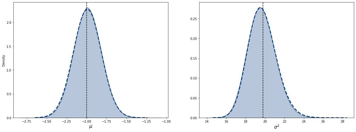
Figure 4: Posterior distribution of $\mu$ and $\sigma^{2}$ for a sample of size $N=1000$, with $m=-2$, $s=3$ such that $\text{med}(X)=m,\text{MAD}(X)=s$ with Robust Gibbs (filled curve) and the approximation $\tilde{\pi}$ (in )dashed blue line). The estimands $m$ and $(c\cdot s)^{2}$ are in black dashed line.

5.2 Cauchy distribution

The sample median and MAD are routinely used as estimators for the location-mean Cauchy distribution, both because the Cauchy’s mean and variance are undefined, and because the location parameter $x_{0}\in\mathbb{R}$ is equal to the theoretical median and the scale parameter $\gamma>0$ is equal to the theoretical MAD (and to the half of the theoretical IQR). The Cauchy distribution serves as a valuable tool for exploring robust statistical methods and understanding their performance under challenging conditions, especially in the presence of heavy-tailed data or outliers. By leveraging the robust estimators of location and scale, we can overcome the limitations posed by traditional measures such as the mean and variance, and obtain more reliable estimates of the parameters of interest.

We conducted a Metropolis-Hastings within Gibbs random walk with Cauchy and Gamma priors on the two parameters. We performed $T$ simulations based on the posterior distribution of the Cauchy parameters $(x_{0},\gamma)$ while observing only the median and the MAD.

Previous studies have resorted to Approximate Bayesian Computation (ABC) to approximate the posterior given the median and MAD [19, 7, 13]. To compare our results, we also carried out simulations using standard ABC methods, using the same observed median and MAD as summary statistics, along with the same non-informative priors. We ran both algorithms for an equal amount of computing time. In ABC, we obtained more than 10 times more simulations by parallelizing the computations. We fixed the threshold by retaining the $T$ best simulations. We thus obtain a fair comparison, with two algorithms run for the same time leading to identical sample sizes. The results of these simulations are presented in Figure 5. Our Robust Gibbs method yields a posterior that is much more peaked around the theoretical parameter values compared to the ABC approach. This is to be expected, since Robust Gibbs samples from the exact posterior, whereas ABC samples from an approximation, which typically inflates the variance.

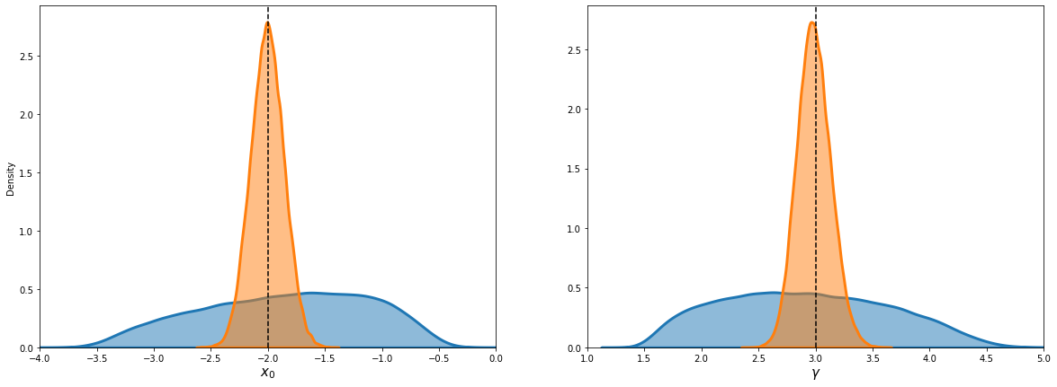
Figure 5: Posterior distributions with true Cauchy parameters $x_{0}=-2$ and $\gamma=3$, and sample size $N=1000$, obtained using the Robust Gibbs method (in orange) and the ABC method (in blue), along with the theoretical values (in black dashed line).

5.3 Weibull Distribution

In this section, we focus on the three-parameter Weibull distribution, also referred to as the translated Weibull distribution. In addition to the classical parameters of scale $\gamma$ and shape $\beta$, this one proposes a parameter of location $x_{0}$. The density of this family of distributions is given by:

$$f(x)=\frac{\beta}{\gamma}\left(\frac{x-x_{0}}{\gamma}\right)^{\beta-1}e^{-(\frac{x-x_{0}}{\gamma})^{\beta}}\mathbb{1}_{x\geq x_{0}}.$$

Bandourian et al [3] recommend this distribution to model the life expectancy or income of individuals..

When we observe a two-dimensional summary statistic $T(X)$, such as the median and exther the MAD or the IQR, the information contained in $T(X)$ does not allow us to identify all three parameters. The median provides information about the location parameter, while the MAD or IQR gives information about the scale parameter. However, there is no direct information about the shape parameter. Therefore, we have an insufficient number of statistics to estimate all three parameters accurately. As a result, our three chains can evolve within a submanifold of $\mathbb{R}^{3}$. However, in cases where the location parameter is fixed (e.g., $x_{0}=0$ for the classical Weibull distribution), we can uniquely identify the scale and shape parameters.

When we consider quantiles as observations, we investigate the impact of the number of quantiles, denoted as $M$, on the posterior distribution. Specifically, we choose the quantile values $(p_{j})_{j=1,\dots,M}$ such that $p_{j}=\frac{j}{M+1}$ for $j=1,\dots,M$. For example, when $M=3$, we have $(p_{1},p_{2},p_{3})=(.25,.5,.75)$, and for $M=9$, we obtain the nine deciles.

As observed in Figure 6, it becomes apparent that using only two quantiles is insufficient to capture all three parameters accurately. However, with a minimum of three quantiles, we can successfully identify all the parameters of the Weibull distribution. Additionally, increasing the number of quantiles leads to a posterior distribution that closely aligns with the theoretical parameters, indicating improved estimation precision.

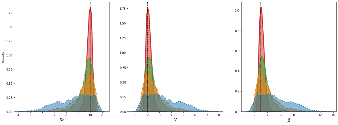
Figure 6: Posterior of the three parameters of the Weibull distribution for a sample of size $N=1000$ given $T(X)=((q_{j})_{j=1,\dots,M},(p_{j})_{j=1,\dots,M})$ where the $(q_{j})$s are the theoretical quantiles of the 3-parameter Weibull distribution with $x_{0}=10$, $\gamma=2$ and $\beta=3$ (black dashed lines) for $M=2$ (blue dotted line), $M=3$ (orange dashed line), $M=4$ (green dashed-dotted line) and $M=9$ (red full line).

6 Conclusion

This paper has presented a novel method for simulating from the posterior distribution when only robust statistics are observed. Our approach, based on Gibbs sampling and the simulation of augmented data as latent variables, offers a versatile tool for a wide range of applied problems. The Python code implementing this method is available as a Python package (https://github.com/AntoineLuciano/Insufficient-Gibbs-Sampling), enabling its application in various domains.

Among the three examples of robust statistics addressed in this paper, two exhibited similarities, where the observed quantiles or the median and interquartile range yielded comparable results to existing methods. The unique case of median absolute deviation (MAD) introduced a novel challenge, for which we proposed a partial data augmentation technique ensuring ergodicity of the Markov chain.

While our focus in this study was on continuous univariate distributions, future research avenues could explore the extension of our method to discrete distributions or multivariate data. These directions promise to further enhance the applicability and generality of our approach.

Appendix A Even case of the median, MAD case

As explained before, the case where $X$ is of even size i.e. $\exists n\geq 4\mbox{ such that }N=2n$ is more complex. Indeed, the statistics that we study are not determined by a single coordinate but by the average of two coordinates of the vector.

It is therefore useful to introduce some extra notations:

• $m_{1}=X_{(n)}$ and $m_{2}=X_{(n+1)}$ where $X_{(k)}$ denotes the k-th order statistic of the vector X, so we have $m=\frac{m_{1}+m_{2}}{2}$.

• $Y=(\lvert X_{i}-m\rvert)_{i=1,\dots,n}$ the vector of distance to the median

• $s_{1}=Y_{(n)}$ and $s_{2}=Y_{(n+1)}$ so we have $s=\frac{s_{1}+s_{2}}{2}$

• $X_{\text{MAD}_{1}}\in X$ such that $\lvert X_{\text{MAD}_{1}}-m\rvert=s_{1}$ and $X_{\text{MAD}_{2}}\in X$ such that $\lvert X_{\text{MAD}_{2}}-m\rvert=s_{2}$

• $\epsilon_{m}=m_{2}-m_{1}$ and $\epsilon_{MAD}=s_{2}-s_{1}$

As for the odd case, we introduce a new partition of $\mathbb{R}$ but this time involving seven intervals presented in 7.

Figure 7: Apportionment of the vector $X$ when $N=2n$ with $n\in\mathbb{N}^{*}$, median$(X)=m$ and MAD$(X)=s$.

The intervals are denoted as follows:

• $Z_{1}=(-\infty,m-s_{2})$

• $Z_{m-s}=(m-s_{2},m-s_{1})$

• $Z_{2}=(m-s_{1},m_{1})$

• $Z_{m}=(m_{1},m_{2})$

• $Z_{3}=(m_{2},m+s_{1})$

• $Z_{m+s}=(m+s_{2},m+s_{1})$

• $Z_{4}=(m+s_{2},+\infty)$

We use the notations from the previous section applied to our new zones. In addition, we introduce:

• An application $S_{y}$ which associates to a point $x$ its symmetric with respect to the point $y$ i.e $S_{y}:x\longrightarrow 2y-x$.

• An application $Zone$ which has a coordinate associates its zone.

• An application $\text{Zone}_{E}$ which has a coordinate associates its “extended” zone to it such that $\text{Zone}_{E}(X)=\left\{\begin{array}[]{ll}(-\infty,m-s)&\mbox{if }X\in Z_{1}\\ (m-s,m_{1})&\mbox{if }X\in Z_{2}\\ (m_{2},m+s)&\mbox{if }X\in Z_{3}\\ (m+s,\infty)&\mbox{if }X\in Z_{4}\\ \end{array}\right.$

• An application $\text{Zone}_{S}$ which has a coordinate associates its “symmetric” zone with respect to $m$ such that $\text{Zone}_{S}(X)=\left\{\begin{array}[]{ll}Z_{4}&\mbox{if }X\in Z_{1}\\ Z_{3}&\mbox{if }X\in Z_{2}\\ Z_{2}&\mbox{if }X\in Z_{3}\\ Z_{1}&\mbox{if }X\in Z_{4}\\ \end{array}\right.$

• An application $\text{Zone}_{C}$ which has a zone associates its “complementary” zone to it such that $\text{Zone}_{C}(X)=\left\{\begin{array}[]{ll}Z_{3}&\mbox{if }X\in Z_{1}\\ Z_{4}&\mbox{if }X\in Z_{2}\\ Z_{1}&\mbox{if }X\in Z_{3}\\ Z_{2}&\mbox{if }X\in Z_{4}\\ \end{array}\right.$

A.1 Methodology

Randomly pick 2 indexes i and j of the vector X

1. If $(X_{i},X_{j})=(m_{1},m_{2})$:

   • $\tilde{X_{i}}\sim\mathcal{F}_{\theta}\mathbb{1}_{[m-Y_{(3)},m+Y_{(3)}]}$

   • $\tilde{X_{j}}=S_{m}(\tilde{X_{i}})$

2. If $(X_{i},X_{j})=(X_{\text{MAD}_{1}},X_{\text{MAD}_{2}})$:

   1. If $X_{i}>m\text{ and }X_{j}>m$:

      • $\tilde{X_{i}}\sim\mathcal{F}_{\theta}\mathbb{1}_{Z_{m+s}^{\prime}}\text{ where }Z_{m+s}^{\prime}=[m+s_{1}-\epsilon,m+s_{2}+\epsilon]\newline \text{and }\epsilon=\min(Y_{(n)}-Y_{(n-1)},Y_{(n+2)}-Y_{(n+1)})$

      • $\tilde{X_{j}}=S_{m+s}(\tilde{X_{i}})$

   2. Elif $X_{i}<m\text{ and }X_{j}<m$:

      • $\tilde{X_{i}}\sim\mathcal{F}_{\theta}\mathbb{1}_{Z_{m-s}^{\prime}}\text{ where }Z_{m-s}^{\prime}=[m-s_{2}-\epsilon,m-s_{1}+\epsilon]\newline \text{and }\epsilon=\min(Y_{(n)}-Y_{(n-1)},Y_{(n+2)}-Y_{(n+1)})$

      • $\tilde{X_{j}}=S_{m-s}(\tilde{X_{i}})$

   3. Else

      • $\tilde{X_{i}}\sim\mathcal{F}_{\theta}\mathbb{1}_{Z_{m-s}^{\prime}\cup Z_{m+s}^{\prime}}$

      • $\tilde{X_{j}}=\left\{\begin{array}[]{ll}S_{m+s}(S_{m}(\tilde{X_{i}}))&\mbox{if }\tilde{X_{i}}>m\\ S_{m-s}(S_{m}(\tilde{X_{i}}))&\mbox{else}\end{array}\right.$

3. If $X_{i}=m_{1}\text{ or }m_{2}\text{ and }X_{j}=X_{\text{MAD}_{1}}\text{ or }X_{\text{MAD}_{2}}$:$\tilde{X_{i}}=X_{i}\text{ and }\tilde{X_{j}}=X_{j}$

4. If $X_{i}=m_{1}\text{ or }m_{2}$:

   1. If $X_{i}=m_{1}$ and $X_{j}\in[m_{2},m-s_{1}]$:

      • $\tilde{X_{i}}\sim\mathcal{F}_{\theta}\mathbb{1}_{[m,m-s_{1}]}$

      • $\tilde{X_{j}}=\left\{\begin{array}[]{ll}S_{m}(\tilde{X_{i}})&\mbox{if }\tilde{X_{i}}\in[m_{1},m_{2}]\\ X_{j}&\mbox{else}\end{array}\right.$

   2. Elif $X_{i}=m_{2}$ and $X_{j}\in[m-s_{1},m_{1}]$:

      • $\tilde{X_{i}}\sim\mathcal{F}_{\theta}\mathbb{1}_{[m-s_{1},m]}$

      • $\tilde{X_{j}}=\left\{\begin{array}[]{ll}S_{m}(\tilde{X_{i}})&\mbox{if }\tilde{X_{i}}\in[m_{1},m_{2}]\\ X_{j}&\mbox{else}\end{array}\right.$

   3. Else: $\tilde{X_{i}}\sim\mathcal{F}_{\theta}\mathbb{1}_{Zone(X_{i})}\text{ and }\tilde{X_{j}}=X_{j}$:

5. If $X_{j}=X_{\text{MAD}_{1}}\text{ or }X_{\text{MAD}_{2}}$:

   1. If $(X_{i}-m)(X_{j}-m)>0$ and $(\lvert X_{i}-m\rvert-s)(\lvert X_{j}-m\rvert-s)<0$:

      • $X_{i}\sim\mathcal{F}_{\theta}\mathbb{1}_{\text{Zone}_{E}(X_{i})}$

      • $\tilde{X_{j}}=\left\{\begin{array}[]{ll}S_{m+s}(\tilde{X_{i}})&\mbox{if }\tilde{X_{i}}\in Z_{m+s}\\ S_{m-s}(\tilde{X_{i}})&\mbox{if }\tilde{X_{i}}\in Z_{m-s}\\ X_{j}&\mbox{else}\end{array}\right.$

   2. Elif $(X_{i}-m)(X_{j}-m)>0$ and $(\lvert X_{i}-m\rvert-s)(\lvert X_{j}-m\rvert-s)>0$:

      • $\tilde{X_{i}}\sim\mathcal{F}_{\theta}\mathbb{1}_{Zone(X_{i})}$

      • $\tilde{X_{j}}=X_{j}$

   3. Elif $(X_{i}-m)(X_{j}-m)<0$ and $(\lvert X_{i}-m\rvert-s)(\lvert X_{j}-m\rvert-s)>0$:

      • $\tilde{X_{i}}\sim\mathcal{F}_{\theta}\mathbb{1}_{Zone(X_{i})\cup\text{Zone}_{S}(X_{i})}$

      • $\tilde{X_{j}}=\left\{\begin{array}[]{ll}X_{j}&\mbox{if }\tilde{X_{i}}\in Zone(X_{i})\\ S_{m}(X_{j})&\mbox{if }\tilde{X_{i}}\in\text{Zone}_{S}(X_{i})\end{array}\right.$

   4. Else:

      • $\tilde{X_{i}}\sim\mathcal{F}_{\theta}\mathbb{1}_{\text{Zone}_{E}(X_{i})}$

      • $\tilde{X_{j}}=\left\{\begin{array}[]{ll}S_{m+s}(S_{m}(\tilde{X_{i}}))&\mbox{if }\tilde{X_{i}}\in Z_{m-s}\\ S_{m-s}(S_{m}(\tilde{X_{i}}))&\mbox{if }\tilde{X_{i}}\in Z_{m+s}\\ X_{j}&\mbox{else}\end{array}\right.$

6. Else:

   1. If $(Zone(X_{i}),Zone(X_{j}))=(Z_{1},Z_{2})$ or $(Z_{3},Z_{4})$:

      • $\tilde{X_{i}}\sim\mathcal{F}_{\theta}\mathbb{1}_{\text{Zone}_{E}(X_{i})\cup\text{Zone}_{E}(X_{j})}$

      • $\left\{\begin{array}[]{ll}\tilde{X_{j}}=S_{m+s}(\tilde{X_{i}})&\mbox{if }\tilde{X_{i}}\in Z_{m+s}\\ \tilde{X_{j}}=S_{m-s}(\tilde{X_{i}})&\mbox{if }\tilde{X_{i}}\in Z_{m-s}\\ \tilde{X_{j}}\sim\mathcal{F}_{\theta}\mathbb{1}_{Zone(X_{j})}&\mbox{if }\tilde{X_{i}}\in Zone(X_{i})\\ \tilde{X_{j}}\sim\mathcal{F}_{\theta}\mathbb{1}_{Zone(X_{i})}&\mbox{else }\end{array}\right.$

   2. Elif $(Zone(X_{i}),Zone(X_{j}))=(Z_{2},Z_{3})$:

      • $\tilde{X_{i}}\sim\mathcal{F}_{\theta}\mathbb{1}_{Z_{2}\cup Z_{m}\cup Z_{3}}$

      • $\left\{\begin{array}[]{ll}\tilde{X_{j}}=S_{m}(\tilde{X_{i}})&\mbox{if }\tilde{X_{i}}\in Z_{m}\\ \tilde{X_{j}}\sim\mathcal{F}_{\theta}\mathbb{1}_{Zone(X_{j})}&\mbox{if }\tilde{X_{i}}\in Zone(X_{i})\\ \tilde{X_{j}}\sim\mathcal{F}_{\theta}\mathbb{1}_{Zone(X_{i})}&\mbox{else }\end{array}\right.$

   3. Elif $(Zone(X_{i}),Zone(X_{j}))=(Z_{1},Z_{3})$ or $(Z_{2},Z_{4})$:

      • $\tilde{X_{i}}\sim\mathcal{F}_{\theta}\mathbb{1}_{\mathbb{R}\ Z_{m}}$

      • $\left\{\begin{array}[]{ll}\tilde{X_{j}}=S_{m+s}(S_{m}(\tilde{X_{i}}))&\mbox{if }\tilde{X_{i}}\in Z_{m-s}\\ \tilde{X_{j}}=S_{m-s}(S_{m}(\tilde{X_{i}}))&\mbox{if }\tilde{X_{i}}\in Z_{m+s}\\ \tilde{X_{j}}\sim\mathcal{F}_{\theta}\mathbb{1}_{\text{Zone}_{C}(\tilde{X_{i}})}&\mbox{else }\end{array}\right.$

   4. Else: $\tilde{X_{i}}\sim\mathcal{F}_{\theta}\mathbb{1}_{Zone(X_{i})}$ and $\tilde{X_{j}}=X_{j}$.

$(X_{i},X_{j})=(\tilde{X_{i}},\tilde{X_{j}})$

Appendix B Proof of Ergodicity for the Chain of Latent Vector $X$

In this section, we prove that our Markov chain on the latent vector $X$ is ergodic. To achieve this, we need to demonstrate its irreducibility and aperiodicity.

Aperiodicity is ensured by the random selection of the coordinates to be resampled and the inherent randomness in the simulation process.

To establish irreducibility, we need to show that all states are reachable within a finite number of iterations. In this regard, we have defined two variables, $k$ and $\delta$, which describe the distribution of observations in the $X$ vector. Therefore, it suffices to demonstrate that we can transition from one state to any other state from this latent space $\mathcal{X}_{m,s}=\{X\in\mathbb{R}^{N}\mid\text{med}(X)=m,\text{MAD}(X)=s\}$.

Let us consider two states of our Markov chain on the latent vector from $\mathcal{X}_{m,s}$, $X$ such that $k(X)=k_{1}\in\{1,\dots,n\}$ and $\delta(X)=\delta_{1}\in\{0,1\}$ to any other state $\tilde{X}$ such that $k(\tilde{X})=k_{2}\in\{1,\dots,n\}$ and $\delta(\tilde{X})=\delta_{2}\in\{0,1\}$.

If $k_{1}\neq k_{2}$, we can assume with no loss of generality that $k_{2}>k_{1}$. In that case, we need to take $k_{2}-k_{1}$ observations in $(-\infty,m-s)$ and $k_{2}-k1$ in $(m,m+s)$ and resample them respectively in $(m-s,m)$ and $(m+s,+\infty)$. This case has a non-zero probability to occur and is described as case 4a in our algorithm.

If $k_{1}=k_{2}$ and $\delta_{1}\neq\delta_{2}$, we need to switch $X_{\text{MAD}}$ from one side of the median to its symmetric side, i.e., $m-s\leftrightarrow m+s$. This case has a non-zero probability to occur and is described as case 3b in our method.

Finally, if $k_{1}=k_{2}$ and $\delta_{1}=\delta_{2}$, $X$ and $\tilde{X}$ present the same distribution between the four intervals introduced previously. We have to resample the observations while maintaining this distribution. This case has a non-zero probability to occur and is described as cases 4b, 3a, and 2 in our method.

By considering these possibilities, we can establish the existence of a non-zero probability for transitioning between any two states in the specified latent space.

Therefore, we have demonstrated the irreducibility of our Markov chain, indicating that it can reach all states within a finite number of iterations.

Appendix C Other median, IQR cases

C.0.1 $N=3\mod 4$

This second case is still an odd case, so the median is still deterministic, and we have $\text{median}(X)=X_{(i_{2})}$. But this time, the two other quartiles are not deterministic. We have $Q_{1}=(1-g_{1})X_{(i_{1})}+g_{1}X_{(i_{1}+1)}$ and $Q_{3}=(1-g_{3})X_{(i_{3})}+g_{3}X_{(i_{3}+1)}$, with $i_{1}=k+1$, $i_{2}=2k+2$, $i_{3}=3k+2$, and $g_{1}=g_{3}=0.5$. We have to consider the joint distribution of five order statistics $X_{(i_{1})},X_{(i_{1}+1)},X_{(i_{2})},X_{(i_{3})},X_{(i_{3}+1)}$ and apply the following transformation $\phi$:

$$\left\{\begin{aligned} Q_{1}&=(1-g_{1})X_{(i_{1})}+g_{1}X_{(i_{1}+1)}\\ m&=X_{(i_{2})}\\ Q_{3}&=(1-g_{3})X_{(i_{3})}+g_{3}X_{(i_{3}+1)}\\ i&=Q_{3}-Q_{1}\end{aligned}\right.\iff\left\{\begin{aligned} X_{(i_{1})}&=X_{(i_{1})}\\ X_{(i_{1}+1)}&=\frac{1}{g_{1}}\left((1-g_{3})X_{(i_{3})}+g_{3}X_{(i_{3}+1)}-(1-g_{1})X_{(i_{1})}-i\right)\\ X_{(i_{2})}&=m\\ X_{(i_{3})}&=X_{(i_{3})}\\ X_{(i_{3}+1)}&=X_{(i_{3}+1)}\end{aligned}\right.$$

In the same way as before, we can sample from the distribution of $X_{(i_{1})},X_{(i_{3})},X_{((i_{3}+1))}\mid\text{med}(X)=m,\text{IQR}(X)=i$ with a step of Metropolis-Hastings.

C.0.2 $N$ is even

In this case, which actually covers two different cases (when $N=4k$ or $N=4k+2$), none of the three quartiles is deterministic. The values of the median and the IQR then depend on six order statistics $X_{(i_{1})},X_{(i_{1}+1)},X_{(i_{2})},X_{(i_{2}+1)},X_{(i_{3})},X_{(i_{3}+1)}$. We have:

$$\left\{\begin{aligned} Q_{1}&=(1-g_{1})X_{(i_{1})}+g_{1}X_{(i_{1}+1)}\\ m&=\frac{X_{(i_{2})}+X_{(i_{2}+1)}}{2}\\ Q_{3}&=(1-g_{3})X_{(i_{3})}+g_{3}X_{(i_{3}+1)}\\ i&=Q_{3}-Q_{1}\end{aligned}\right.\iff\left\{\begin{aligned} X_{(i_{1})}&=X_{(i_{1})}\\ X_{(i_{1}+1)}&=\frac{1}{g_{1}}\left((1-g_{3})X_{(i_{3})}+g_{3}X_{(i_{3}+1)}-(1-g_{1})X_{(i_{1})}-i\right)\\ X_{(i_{2})}&=X_{(i_{2})}\\ X_{(i_{2}+1)}&=2m-X_{(i_{2})}\\ X_{(i_{3})}&=X_{(i_{3})}\\ X_{(i_{3}+1)}&=X_{(i_{3}+1)}\end{aligned}\right.$$

When $N=4k$, we have $i_{1}=k$, $i_{2}=2k$, $i_{3}=3k$, $g_{1}=0.75$, and $g_{3}=0.25$. When $N=4k+2$, we have $i_{1}=k+1$, $i_{2}=2k+1$, $i_{3}=3k+1$, $g_{1}=0.25$, and $g_{3}=0.75$.

Thanks to this transformation, we can sample from $X_{(i_{1})},X_{(i_{2})},X_{(i_{3})},X_{((i_{3}+1))}\mid\text{med}(X)=m,\text{IQR}(X)=i$ with a step of Metropolis-Hastings within Gibbs.

References

- \bibcommenthead
- Akinshin [2022] Akinshin A (2022) Quantile absolute deviation. 10.48550/arXiv.2208.13459, 2208.13459[stat]
- Baglivo [2005] Baglivo JA (2005) Mathematica Laboratories for Mathematical Statistics. Society for Industrial and Applied Mathematics, Philadelphia, PA, USA, 10.1137/1.9780898718416
- Bandourian et al [2002] Bandourian R, McDonald J, Turley RS (2002) A comparison of parametric models of income distribution across countries and over time. Working Paper No. 305, Luxembourg income study working paper, 10.2139/ssrn.324900
- David and Nagaraja [2004] David HA, Nagaraja HN (2004) Order Statistics. John Wiley & Sons, New Jersey, NJ, USA
- Frazier et al [2020] Frazier DT, Robert CP, Rousseau J (2020) Model misspecification in approximate bayesian computation: consequences and diagnostics. Journal of the Royal Statistical Society Series B: Statistical Methodology 82(2):421–444. 1708.01974
- Gauss [1816] Gauss CF (1816) Bestimmung der Genauigkeit der Beobachtungen. Zeitschrift für Astronomie und verwandte Wissenschaften URL https://cir.nii.ac.jp/crid/1571417124784507520
- Green et al [2015] Green PJ, Łatuszyński K, Pereyra M, et al (2015) Bayesian computation: a summary of the current state, and samples backwards and forwards. Statistics and Computing 25(4):835–862. 10.1007/s11222-015-9574-5
- Hampel [1968] Hampel FR (1968) Contributions to the Theory of Robust Estimation. University of California, California, CA, USA
- Hampel [1974] Hampel FR (1974) The Influence Curve and Its Role in Robust Estimation. Journal of the American Statistical Association 69(346):383–393. 10.1080/01621459.1974.10482962
- Huang et al [2023] Huang D, Bharti A, Souza A, et al (2023) Learning Robust Statistics for Simulation-based Inference under Model Misspecification. 10.48550/arXiv.2305.15871, arXiv:2305.15871 [cs, stat]
- Huber [1964] Huber PJ (1964) Robust estimation of a location parameter. Annals of Mathematical Statistics 35:73–101. 10.1214/aoms/1177703732
- Hyndman and Fan [1996] Hyndman RJ, Fan Y (1996) Sample Quantiles in Statistical Packages. The American Statistician 50(4):361–365. 10.2307/2684934
- Marin et al [2014] Marin JM, Pillai NS, Robert CP, et al (2014) Relevant statistics for Bayesian model choice. Journal of the Royal Statistical Society Series B (Statistical Methodology) 76(5):833–859. 10.1111/rssb.12056
- McVinish [2012] McVinish R (2012) Improving ABC for quantile distributions. Statistics and Computing 22(6):1199–1207. 10.1007/s11222-010-9209-9
- Nirwan and Bertschinger [2022] Nirwan RS, Bertschinger N (2022) Bayesian Quantile Matching Estimation. URL http://arxiv.org/abs/2008.06423, arXiv:2008.06423 [stat]
- Rousseeuw and Croux [1993] Rousseeuw PJ, Croux C (1993) Alternatives to the Median Absolute Deviation. Journal of the American Statistical Association 88(424):1273–1283. 10.1080/01621459.1993.10476408
- Tanner and Wong [1987] Tanner MA, Wong WH (1987) The Calculation of Posterior Distributions by Data Augmentation. Journal of the American Statistical Association 82(398):528–540. 10.2307/2289457
- Tukey [1960] Tukey JW (1960) A survey of sampling from contaminated distributions. Contributions to Probability and Statistics pp 448–485
- Turner and Van Zandt [2012] Turner BM, Van Zandt T (2012) A tutorial on approximate Bayesian computation. Journal of Mathematical Psychology 56:69–85. 10.1016/j.jmp.2012.02.005