Interlayer Coupling Driven High-Temperature Superconductivity in La₃Ni₂O₇ Under Pressure

Abstract

The newly discovered high-temperature superconductivity in La₃Ni₂O₇ under pressure has attracted a great deal of interests. The essential ingredient characterizing the electronic properties is the bilayer NiO₂ planes, in which the two layers couple with each other from the bonding of Ni-$3d_{z^{2}}$ orbital through the intermediate oxygen-atoms. In the strong coupling limit, an intralayer antiferromagnetic spin-exchange interaction $J_{\parallel}$ between $3d_{x^{2}-y^{2}}$ orbitals and an interlayer one $J_{\perp}$ between $3d_{z^{2}}$ orbitals are generated. Taking into account the Hund’s rule at each site and integrating out the $3d_{z^{2}}$ spin degree of freedom, the system reduces to a single-orbital bilayer $t$-$J$ model of the $3d_{x^{2}-y^{2}}$. Based on the slave-boson approach, the self-consistent equation for the hopping and pairing order parameters is solved. Near the relevant $\frac{1}{4}$-filling regime (doping $\delta=0.3\sim 0.5$), the inter-layer coupling $J_{\perp}$ tunes the conventional single-layer $d$-wave superconducting state to the $s$-wave one. A strong $J_{\perp}$ could enhance the inter-layer superconducting order, leading to a dramatically increased $T_{c}$. Interestingly, there could exist a finite regime in which an $s+id$ state emerges.

Introduction: Since the discovery of the high-temperature superconductivity (SC) in cuprates Bednorz and Müller (1986); Anderson (1987), understanding the pairing mechanism of unconventional SC Anderson (1987); Kotliar and Liu (1988); Lee et al. (2006); Keimer et al. (2015); Proust and Taillefer (2019) and searching for new superconductors with high critical temperature $T_{c}$ remain long-term challenges. It has been widely believed that strong electron correlations drive the $d$-wave pairing symmetry in the high-$T_{c}$ SC Anderson (1987); Kotliar and Liu (1988); Lee et al. (2006). Under such a understanding, many attempts have been made to search for high-$T_{c}$ SCs in materials with strong electron correlations, especially, the 3d-transition metal oxidesAnisimov et al. (1999); Li et al. (2019); Hu and Wu (2019); Zhang et al. (2020); Botana et al. (2021); Zeng et al. (2022); Lu et al. (2022). However, no new superconductors family with $T_{c}$ above the boiling point of liquid nitrogen was synthesized until the recent discovery of SC with $T_{c}=80$K in the La₃Ni₂O₇ (LNO) under a pressure of over $14$GPa Sun et al. (2023), which has attracted many experimental Liu et al. (2023a); Hou et al. (2023) and theoretical attentions Luo et al. (2023); Zhang et al. (2023); Yang et al. (2023); Sakakibara et al. (2023); Gu et al. (2023); Shen et al. (2023); Wú et al. (2023); Christiansson et al. (2023); Liu et al. (2023b).

Similarly to cuprates, the LNO hosts a layered structure Sun et al. (2023); Hou et al. (2023); Liu et al. (2023a) with each unit cell containing two conducting NiO₂ layers, which is isostructure with the CuO₂ layer in cuprates. Calculations based on density-functional-theory (DFT) Pardo and Pickett (2011); Sun et al. (2023) suggest that the low-energy degrees of freedom near the Fermi level are of the Ni-3$d$ orbitals, including two $E_{g}$ orbitals, i.e., $3d_{z^{2}}$ and $3d_{x^{2}-y^{2}}$, with the site energy of the former lower than that of the latter. Four $E_{g}$ orbitals in two Ni^2.5+ cations within a unit cell share three electrons in total. The $3d_{z^{2}}$ orbitals in two layers within a unit cell couple via the hybridization with the O-$2p$ orbitals in the intercalated LaO layer. Under pressure, such a Ni-O-Ni bonding angle along the $c$-axis changes from 168^∘ to 180^∘. This largely enhances the effective interlayer coupling, under which the high-$T_{c}$ SC emerges Sun et al. (2023). It implies that the interlayer coupling is crucial for the high-$T_{c}$ SC in the LNOLiu et al. (2023b).

The $3d$-orbital character of the low-energy degrees of freedom in the LNO suggests that electron correlation in this material is strong. Such a viewpoint is supported by a recent experimentLiu et al. (2023a) which revealed that the LNO system is near the boundary of the Mott transition. Therefore, the strong-coupling picture should be legitimate towards the pairing mechanism therein. It has been proposed in Ref. Shen et al. (2023); Wú et al. (2023) that the interlayer coupling between the two Ni-$3d_{z^{2}}$ orbitals along the rung within a unit cell would induce antiferromagnetic (AFM) super exchange interactions. The same viewpoint is adopted here. However, an important ingredient has been missed in these studies, i.e. the Hund’s rule coupling between the $3d_{z^{2}}$ and the $3d_{x^{2}-y^{2}}$ orbitals within the same Ni^2.5+ cations, whose effect will be considered in the present study.

In this Letter, strongly-correlated models are built to study the pairing mechanism and pairing nature of LNO under pressure. We start from the fact that, the three electrons within each unit cell would first fill in the two $3d_{z^{2}}$ orbitals, which would finally be half filled due to the strong Hubbard repulsion. Hence we are left with two half-filled $3d_{z^{2}}$ orbitals and two quarter-filled $3d_{x^{2}-y^{2}}$ orbitals in each unit cell. The two half-filled $3d_{z^{2}}$ orbitals in a unit cell can be viewed as two insulating spins which couple via the interlayer AFM superexchange interaction $J_{\perp}$Shen et al. (2023); Wú et al. (2023), while the two quarter-filled $3d_{x^{2}-y^{2}}$ orbitals take the role of charge carrier. Under Hund’s rule coupling, the AFM interlayer super-exchange interaction between two $3d_{z^{2}}$ orbitals is transmitted to that between two $3d_{x^{2}-y^{2}}$ orbitals in a unit cell. In combination with the intralayer super-exchange interaction, we arrive at a bilayer $t$-$J$ model for the single $3d_{x^{2}-y^{2}}$ orbital, which is responsible for the SC in LNO. Within the slave-boson mean-field (SBMF) theory Kotliar and Liu (1988); Lee et al. (2006), this model is solved to obtain the ground-state phase diagram and the superconducting $T_{c}$. Our result suggests that in the doping regime relevant to experiments, the original intra-layer $d$-wave pairing for $J_{\perp}=0$ is changed into the inter-layer $s$-wave pairing by realistic $J_{\perp}$. In a finite regime between the two pairing symmetries in the phase diagram, a time-reversal-symmetry breaking (TRSB) $s+id$-wave pairing emerges. Adopting realistic parameters obtained from DFT calculationsSun et al. (2023); Luo et al. (2023), our results reveal that $T_{c}$ is dramatically enhanced by the interlayer AFM coupling relative to that for the single-layered case, which may well explain the origin of the high $T_{c}$ SC observed in LNO under pressureSun et al. (2023). Our results further suggest that electron doping into the material will largely enhance $T_{c}$.

Model: On average the electron numbers in each $3d_{z^{2}}$ orbital and $3d_{x^{2}-y^{2}}$ orbital are 1 and 0.5, corresponding to half-filling and $1/4$ filling respectively. Due to Hund’s rule, the electrons in $3d_{z^{2}}$ and $3d_{x^{2}-y^{2}}$ orbitals on ths same Ni site tend to form a spin-triplet state. The $3d_{x^{2}-y^{2}}$ orbital lies within the NiO₂ and its interlayer hopping $t_{\perp}$ nearly vanishes. The two layers couple with each other through the electron hopping of $3d_{z^{2}}$ orbital, inter-mediated by the $2p$ orbital of inter O-atom. The hopping strength could be enhanced under pressure Liu et al. (2023b). In the strong coupling limit, superexchange mechanism induces an effective interlayer AFM spin-exchange $J_{\perp}$ between the two $3d_{z^{2}}$ electrons Shen et al. (2023); Wú et al. (2023). Electronic properties are characterized by a two $E_{g}$-orbitals bilayer $t-J-J_{H}$ model, as depicted in Fig. 1(a).

The Hamiltonian of the model is $H=H_{\parallel}+H_{\perp}$, with

$$H_{\parallel}= -t\sum_{\langle\bm{i},\bm{j}\rangle,\alpha,\sigma}\big{(}{c}^{\dagger}_{\bm{i}\alpha\sigma}{c}_{\bm{j}\alpha\sigma}+\text{h.c.}\big{)}+J_{\parallel}\sum_{\langle\bm{i},\bm{j}\rangle,\alpha}\bm{S}_{\bm{i}\alpha}\cdot\bm{S}_{\bm{j}\alpha}$$

$$H_{\perp}= -J_{H}\sum_{\bm{i},\alpha}\bm{S}_{\bm{i}\alpha}\cdot\bm{S}_{z^{2}\bm{i}\alpha}+J_{\perp}\sum_{\bm{i}}\bm{S}_{z^{2}\bm{i}1}\cdot\bm{S}_{z^{2}\bm{i}2}.$$ (1)

Here $c_{\bm{i}\alpha\sigma}^{\dagger}$ creats a 3$d_{x^{2}-y^{2}}$ electron with spin $\sigma$ at lattice sites $\bm{i}$ in the layer $\alpha=1,2$. $\bm{S}_{\bm{i}\alpha}=\frac{1}{2}c_{\bm{i}\alpha\sigma}^{\dagger}[\bm{\sigma}]_{\sigma\sigma^{\prime}}c_{\bm{i}\alpha\sigma^{\prime}}$ is the spin operator for the $d_{x^{2}-y^{2}}$ orbital, with Pauli matrix $\bm{\sigma}=(\sigma_{x},\sigma_{y},\sigma_{z})$. The summation $\langle\bm{i}\bm{j}\rangle$ takes over all the nearest-neighboring (NN) bonds. Hence, the $H_{\parallel}$ describes two separate layers of conventional $t$-$J$ model of $3d_{x^{2}-y^{2}}$ electrons with a hopping $t$ term and an AFM spin-exchange $J_{\parallel}$ term. The $\bm{S}_{z^{2}\bm{i}\alpha}$ is the spin operator of the localized single-occupied $3d_{z^{2}}$ orbital. Therefore, the $H_{\perp}$ describes the coupling of the two $t$-$J$ layers through the Hund’s rule coupling $J_{H}$ between the two $E_{g}$-orbitals and the interlayer AFM super-exchange $J_{\perp}$ between the $3d_{z^{2}}$-orbital spins within the two layers.

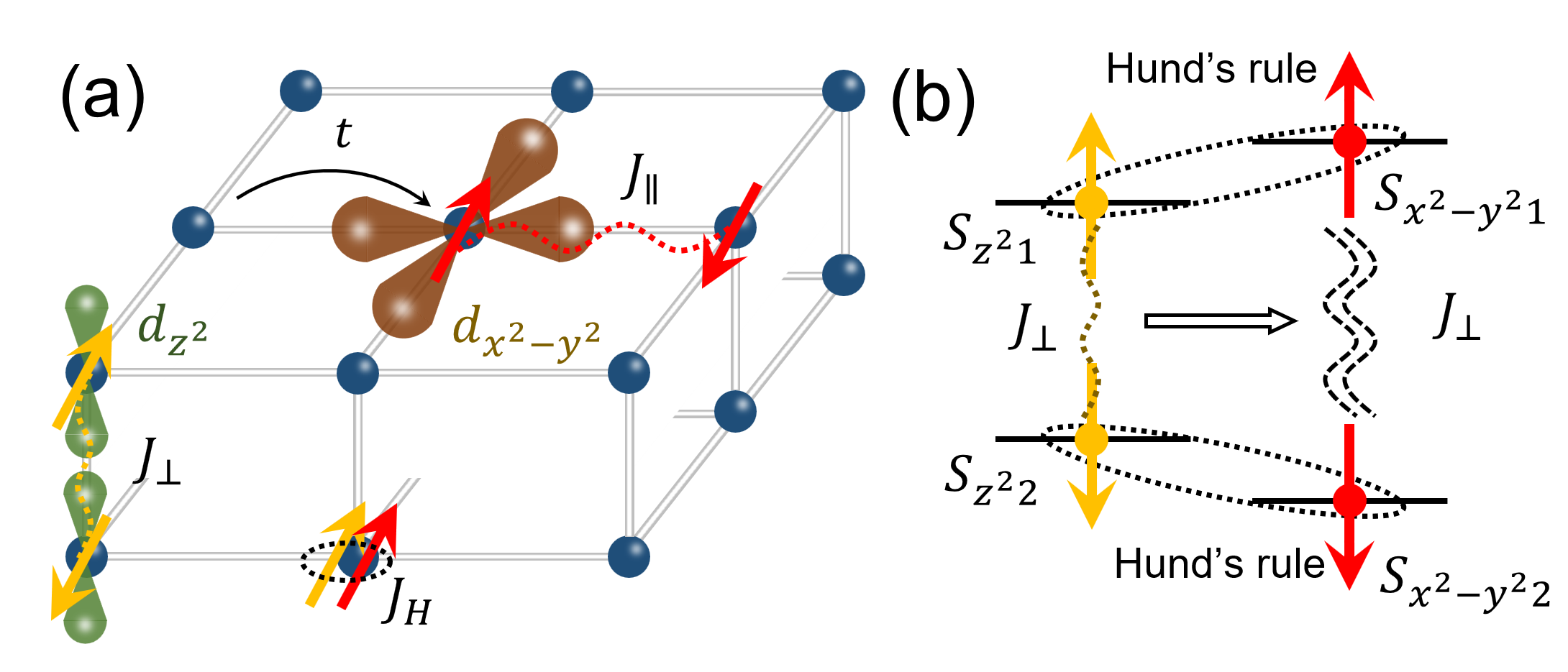
Figure 1: (a). Schematic diagram for the two-orbital bilayer $t-J-J_{H}$ model. The charge carriers reside on the $3d_{x^{2}-y^{2}}$ orbitals, with intra-layer hopping $t$ and spin exchange $J_{\parallel}$. The $3d_{z^{2}}$ orbital is a singly-occupied spin, with inter-layer spin exchange $J_{\perp}$. At each site, the two $E_{g}$ orbitals tend to form a spin-triplet due to Hund’s rule ($J_{H}$). (b). Schematic diagram showing the effective $3d_{x^{2}-y^{2}}$ orbital interlayer spin-exchange $J_{\perp}\bm{S}_{x^{2}-y^{2}1}\cdot\bm{S}_{x^{2}-y^{2}2}$, induced from the combined effect of Hund’s rule coupling and spin exchange $J_{\perp}\bm{S}_{z^{2}1}\cdot\bm{S}_{z^{2}2}$ for a pair of sites $1,2$ in the two layers within a unit cell.

This two orbital problem can be further simplified into a single $3d_{x^{2}-y^{2}}$-orbital one due to Hund’s rule, which constitutes a minimal model for the mechanism of SC. In the semi-classical picture, strong Hund’s coupling $J_{H}$ forces the $3d_{x^{2}-y^{2}}$ spins $\bm{S}_{\bm{i}\alpha}$ aligning in the directions of $\bm{S}_{z^{2}\bm{i}\alpha}$. Integrating out the spin degree of freedom of the $3d_{z^{2}}$ orbital $\bm{S}_{z^{2}\bm{i}\alpha}$ based on the spin-coherent-state path integral Auerbach (1998), an effective interlayer spin-exchange between $3d_{x^{2}-y^{2}}$ electrons emerges (as depicted in Fig. 1(b), see Appendix A). This insight can also be understood in the operator formulism: In the large $J_{H}$ limit, the $3d_{x^{2}-y^{2}}$ and $3d_{z^{2}}$ orbitals on the same Ni^2.5+ cation form a spin-1. When acting on this restricted Hilbert space, the spin exchange interaction $\bm{S}_{z^{2}1}\cdot\bm{S}_{z^{2}2}$ is equivalent to $\bm{S}_{1}\cdot\bm{S}_{2}$, as proved in Appendix B. The remaining theory is a bilayer single $3d_{x^{2}-y^{2}}$-orbital $t$-$J$ model with the nearest-neighbor spin exchange,

$$H=-t\sum_{\langle\bm{i},\bm{j}\rangle,\alpha,\sigma}\big{(}{c}^{\dagger}_{\bm{i}\alpha\sigma}{c}_{\bm{j}\alpha\sigma}+\text{h.c.}\big{)}+J_{\parallel}\sum_{\langle\bm{i},\bm{j}\rangle,\alpha}\bm{S}_{\bm{i}\alpha}\cdot\bm{S}_{\bm{j}\alpha}$$

$$-t_{\perp}\sum_{\bm{i}\sigma}\big{(}{c}^{\dagger}_{\bm{i}1\sigma}{c}_{\bm{i}2\sigma}+\text{h.c.}\big{)}+J_{\perp}\sum_{\bm{i}}\bm{S}_{\bm{i}1}\cdot\bm{S}_{\bm{i}2},$$ (2)

where the interlayer interaction is larger than the intralayer one, $J_{\perp}>J_{\parallel}$. A small inter-layer hopping $t_{\perp}(\simeq 0.01t-0.05t)$ is added to pin down the relative pairing phase between the two layers.

The ground-state phase diagram: We adopt the SBMF theoryKotliar and Liu (1988); Lee et al. (2006) to treat with the above bilayer $t$-$J$ model (Interlayer Coupling Driven High-Temperature Superconductivity in La₃Ni₂O₇ Under Pressure) (see Appendix.C for details). The electron operator is decomposed into $c_{i\alpha\sigma}^{\dagger}=f_{i\alpha\sigma}^{\dagger}b_{i\alpha}$, where $f_{i\alpha\sigma}^{\dagger}/b_{i\alpha}$ is the creation/annilation operator of spinon/holon. At the MF level, the spinon and holon degrees of freedom are decoupled. In the ground state, the holons are Bose-Einstein condensed (BEC), and thus its operator can be simplified as $b_{i\alpha}=\sqrt{\delta}$, where the hole-doping level $\delta$ is defined as twice of the deviation from half filling and is related to the filling fraction $x$ as $\delta=1-2x$. In the ideal case, the filling fraction should be $x=0.25$. However, in realistic materials, considering the overlap between the $3d_{x^{2}-y^{2}}$ band and the $3d_{z^{2}}$ band, as well as the fact that some holes can reside on the O-anionsWú et al. (2023), the filling fraction can be above $0.25$. In our calculation, we set $x\in(0.25,0.35)$, corresponding to $\delta\in(0.3,0.5)$. Note that for the single-layer $t$-$J$ model, the pairing strength in such a heavily overdoped region is very weak.

The super-exchange terms in Eq. (Interlayer Coupling Driven High-Temperature Superconductivity in La₃Ni₂O₇ Under Pressure) can be decomposed by the following intra- and inter- layer bonding and pairing order parameters,

$$\chi_{\bm{i}\bm{j}}^{(\alpha)}= \langle f_{\bm{j}\alpha\uparrow}^{\dagger}f_{\bm{i}\alpha\uparrow}+f_{\bm{j}\alpha\downarrow}^{\dagger}f_{\bm{i}\alpha\downarrow}\rangle\equiv\chi_{\bm{j}-\bm{i}}^{(\alpha)},$$ (3)

$$\Delta_{\bm{i}\bm{j}}^{(\alpha)}= \langle f_{\bm{j}\alpha\downarrow}f_{\bm{i}\alpha\uparrow}-f_{\bm{j}\alpha\uparrow}f_{\bm{i}\alpha\downarrow}\rangle\equiv\Delta_{\bm{j}-\bm{i}}^{(\alpha)},$$

$$\chi_{\bm{i},\perp}= \langle f_{\bm{i}2\uparrow}^{\dagger}f_{\bm{i}1\uparrow}+f_{\bm{i}2\downarrow}^{\dagger}f_{\bm{i}1\downarrow}\rangle\equiv\chi_{z},$$

$$\Delta_{\bm{i},\perp}= \langle f_{\bm{i}2\downarrow}f_{\bm{i}1\uparrow}-f_{\bm{i}2\uparrow}f_{\bm{i}1\downarrow}\rangle\equiv\Delta_{z},$$

which are assumed to be site-independent. The three pairing order parameters are marked in the inset of Fig. 2.

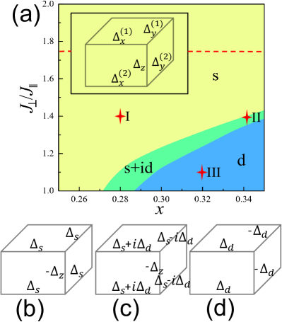
Figure 2: (a) Ground state phase diagram with respect to the filling $x$ and $J_{\perp}/J_{\parallel}$ with $J_{\parallel}=0.4t$. The inset shows the pairing order parameters. At point I (0.28,1.4): $\Delta_{z}=3.1\times 10^{-3}$, $\Delta^{(1,2)}_{x}=\Delta^{(1,2)}_{y}=-1.6\times 10^{-4}$. At point II (0.342,1.39): $\Delta_{z}=3.9\times 10^{-2}$, $\Delta^{(1,2)}_{x}=\Delta^{(1,2)*}_{y}=(-1.2+2.7i)\times 10^{-3}$. At point III (0.32,1.1): $\Delta_{z}$=0, $\Delta^{(1,2)}_{x}=-\Delta^{(1,2)}_{y}=4.1\times 10^{-3}$. The red dashed line marks the realistic $J_{\perp}/J_{\parallel}\approx 1.75$ for LNO. (b-d) show the pairing configurations of the $s$-wave (I), $s+id$-wave (II) and $d$-wave (III), respectively.

The ground-state phase diagram with respect to the filling $x$ and $J_{\perp}/J_{\parallel}$ is shown in Fig. 2(a). Here we have set $J_{\parallel}=0.4t$, and other $J_{\parallel}$ will yield qualitatively similar result. As $J_{\perp}$ should be larger than $J_{\parallel}$, we have set $J_{\perp}/J_{\parallel}\in(1,2)$ in the phase diagram. Three different phases exist in Fig. 2(a). The lower right region (defined as region III) wherein the filling is relatively high and $J_{\perp}/J_{\parallel}$ is relatively small is occupied by the $d$-wave pairing. This region can be continuously connected to the low hole-doped case for the single-layered $t$-$J$ modelKotliar and Liu (1988) representing the cuprates. The upper left region wherein the filling is relatively low and $J_{\perp}/J_{\parallel}$ is relatively large (defined as region I) is occupied by the $s$-wave pairing. This region is relevant to LNO, wherein $J_{\perp}/J_{\parallel}\approx 1.75$ (red dashed line), see the estimation below. A variant of the bilayer Hubbard model augmented by a strong inter-layer super-exchange reaching the order of Hubbard $U$ has been simulated by quantum Monte-Carlo simulation free of the sign problem, which also shows the extended $s$-wave pairing Ma et al. (2022). It is interesting to note that the narrow region (defined as region II) sitting in between region I and III is occupied by the TRSB $s+id$-wave pairing.

To gain more information of the pairing nature, one typical point is taken within each region in Fig. 2(a) to provide the pairing configurations. At the typical point in region I showing the $s$-wave pairing, $\Delta_{z}=3.1\times 10^{-3}$, $\Delta^{(1,2)}_{x}=\Delta^{(1,2)}_{y}=-1.6\times 10^{-4}$, schematically shown in Fig. 2(b). Consequently, the order parameters in the two layers are in phase, and the interlayer pairing dominates the intralayer one. It is interesting to note that $\Delta_{z}$ and $\Delta^{(1,2)}_{x,y}$ hold different signs, which can be thought as the residue of the $d$-wave pairing from the side view. At the typical point in region III exhibiting the $d$-wave pairing, $\Delta_{z}$=0, $\Delta^{(1,2)}_{x}=-\Delta^{(1,2)}_{y}=4.1\times 10^{-3}$, schematically shown in Fig. 2(d). It turns out that the $d$-wave pairing order parameters on the two layers are in phase, and the interlayer pairing vanishes as it is inconsistent with this symmetry. At the typical point in region II exhibiting the $s+id$-wave pairing, $\Delta_{z}=3.9\times 10^{-2}$, $\Delta^{(1,2)}_{x}=\Delta^{(1,2)*}_{y}=(-1.2+2.7i)\times 10^{-3}$. This pairing configuration is schematically shown in Fig. 2(c), which can be decomposed as $\Delta_{s}+i\Delta_{d}$, wherein the schematic pairing configurations for $\Delta_{s}$ and $\Delta_{d}$ are the same as Fig. 2(b) and (d). The $s+id$ pairing state in the intermediate regime spontaneously breaks the time-reversal symmetry. Similar $s+id$ state has been suggested in the much larger filling (or much lower doping) and much smaller $J_{\perp}$ regimeSuzumura et al. (1988); Kuboki and A. Lee (1995); Zhao and Engelbrecht (2005). Such a state could induce non-trivial supercurrent due to spatial inhomogeneity, which can be experimentally detected Lee et al. (2009).

High-T_c SC driven by interlayer coupling: In the SBMF, the onset of SC requires that the holons condense and the spinons pair. Therefore, the superconducting $T_{c}$ is determined by the minimum of $T_{\text{BEC}}$ and $T_{\text{RVB}}$, where $T_{\text{BEC}}$ represents the BEC temperature of the holons and $T_{\text{RVB}}$ indicates the pairing temperature of the spinons. As the hole-doping level $\delta$ is very large, $T_{\text{BEC}}\gg T_{\text{RVB}}$Kotliar and Liu (1988), and hence $T_{c}=T_{\text{RVB}}$, which can be obtained by solving the finite-temperature MF self-consistent gap equation.

The obtained $T_{c}$ as function of the filling $x$ is shown in Fig. 3 (a) for various different interlayer super-exchange strengths $J_{\perp}$, with $J_{\perp}/J_{\parallel}=1,1.5,2,2.5,3$ in comparison with the case of $J_{\perp}=0$. Obviously, the $T_{c}$ rises promptly with the enhancement of $x$ near $x=0.25$ for whatever $J_{\perp}/J_{\parallel}$. This feature is similar with the case of $J_{\perp}=0$ representing the single-layer $t$-$J$ model, wherein $T_{c}$ drops promptly when the hole-doping $\delta$ approaches $\delta=0.5$. The $T_{c}$ as function of $J_{\perp}/J_{\parallel}$ is shown in Fig. 3 (b) for the fillings $x=0.25,0.28,0.3,0.32$. Remarkably, the $T_{c}$ for all these experimentally relevant fillings increase monotonically and drastically with the enhancement of $J_{\perp}/J_{\parallel}$ for $J_{\perp}>J_{\parallel}$. The results shown in Fig. 3 (a-b) are consistent with two important experiment facts. Firstly, the LNO is not superconducting in ambient pressure while high-$T_{c}$ SC emerges under pressure, as pressure enhances the interlayer coupling, and hence $J_{\perp}$. Secondly, the apical-oxygen vacancies suppress SC promptly. In our theory, this is because these vacancies break the Ni-O-Ni bonding along the z-axis, and hence $J_{\perp}$ vanishes locally, which is harmful for SC. Fig. 3 (a-b) further indicate that electron doping into LNO will effectively enhance $T_{c}$, while hole doping will suppress $T_{c}$.

In LNO, the interlayer hopping integral of the $d_{z^{2}}$ orbital is about 0.635 eV and the intralayer NN hopping integral of the $d_{x^{2}-y^{2}}$ is about 0.48 eVLuo et al. (2023), then $J_{\perp}/J_{\parallel}\approx(0.635/0.48)^{2}\approx 1.75$, as the Hubbard $U$ of the two orbitals are near. Fig. 3(c) shows the comparison of the filling dependence of $T_{c}$ between $J_{\perp}=0$ and the realistic $J_{\perp}$, which suggests that near $x=0.25$, the $T_{c}$ at $J_{\perp}/J_{\parallel}=1.75$ is more than an order of magnitude higher than that at $J_{\perp}=0$. The pairing symmetry for $J_{\perp}/J_{\parallel}=1.75$ in experiment relevant filling regime is $s$-wave, consistent with Fig. 2 (a). The corresponding pairing configuration is shown in Fig. 3 (d), wherein we have $\Delta_{x}\approx 0$. Therefore, for these realistic parameters in LNO, the pairing state is the interlayer $s$-wave pairing. Here the interlayer pairing is favored over the intralayer one as the former suffers from less “pairing frustration” than the latter: Taking an electron at the top layer, if it chooses intralayer pairing, it has to choose one among the four surrounding NN sites to pair, which compete and frustrate one another. If instead it chooses interlayer pairing, it can focus on the only one site at the bottom layer to pair. This not only makes $\Delta_{z}\gg\Delta_{x}$, but also largely enhances $\Delta_{z}$ due to reduced “pairing frustration”. Therefore, the interlayer pairing mechanism leads to interlayer s-wave pairing with largely enhanced $T_{c}$.

Besides the interlayer pairing mechanism, the two-orbital character is also crucial for the high-Tc SC of LNO. Suppose we try to realize the bilayer t-J model studied here by a single-orbital bilayer material, wherein the intra- (inter-) layer hopping integral $t_{\parallel}$ ($t_{\perp}$) induces the intra- (inter-) layer super-exchange $J_{\parallel}$ ($J_{\perp}$), satisfying $J_{\perp}/J_{\parallel}\approx(t_{\perp}/t_{\parallel})^{2}$Nazarenko and Dagotto (1996). To mimics such a material, we tune $t_{\perp}$ accordingly, and re-investigate the problem. Consequently, due to change of the band structure caused by the enhanced $t_{\perp}$, the effect of the enhanced $J_{\perp}$ on $T_{c}$ becomes elusive, which cannot drastically enhance $T_{c}$. Here in LNO, it is ingenious that although the conducting $d_{x^{2}-y^{2}}$ orbitals provide very weak $t_{\perp}$, it can acquire strong effective $J_{\perp}$ transmitted from the $d_{z^{2}}$ orbital via the Hund’s rule coupling. Then it is possible to unilaterally enhance $J_{\perp}$ without enhancing $t_{\perp}$ accordingly in this effective single-orbital model through imposing pressure, under which the $T_{c}$ can be drastically enhanced. Therefore, the Hund’s-rule-coupled two-orbital character is crucial to realize the high-Tc SC in LNO.

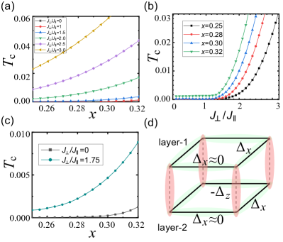
Figure 3: (a) Superconducting $T_{c}$ versus filling $x$ at $J_{\parallel}=0.4t$ for different coupling ratios $J_{\perp}/J_{\parallel}=0,1,1.5,2,2.5,3$. (b) $T_{c}$ versus $J_{\perp}/J_{\parallel}$ for different filling $x=0.25,0.28,0.3,0.32$.(c) Comparison of $T_{c}$ versus filling $x$ between $J_{\perp}/J_{\parallel}=0$ and $J_{\perp}/J_{\parallel}=1.75$. (d) Pairing configuration of the obtained interlayer-s-wave pairing for $J_{\perp}/J_{\parallel}=1.75$.

Discussion and Conclusion: Different from the cuprates, there is no pseudo gap phase for the realistic parameters of LNO, as the doping level $\delta\approx 0.5$ locates well within the heavily overdoped region, in which $T_{\text{BEC}}\gg T_{\text{RVB}}$. However, if we further enhance $J_{\perp}$ so that the interlayer pairing gap energy overwhelms the intralayer hopping energy, an electron from the top layer would tightly pair with another electron from the bottom layer at the same site to form a local Boson at a very high $T_{\text{RVB}}$ (i.e. $T^{*}$), which will then experience a BEC at a lower temperature $T_{\text{BEC}}$ (i.e. $T_{c}$) to form the SC. In such a case, the phase between $T^{*}$ and $T_{c}$ is the pseudo gap phase. Such interesting physics might be realized through further enhancing the pressure.

An interesting possibility of LNO is the charge-4e SC. This originates from the $U(1)\times U(1)$ gauge symmetry for vanishing $t_{\perp}$. If we tune the doping so that the system locates within the d-wave pairing phase, the phase difference between the top and bottom layer is determined by the sign of the vanishing $t_{\perp}$, which will strongly fluctuate at finite temperature. It’s possible that above the pairing $T_{c}$, while the relative phase difference between the two layers is not locked, their total phase is locked, leading to the charge-4e SC. Such exotic SC can be detected by half magnetic flux quantization.

In conclusion, we have derived an effective bilayer $t-J$ model to describe the charge carriers on the Ni-$3d_{x^{2}-y^{2}}$ orbitals with filling fraction near $\frac{1}{4}$, which are responsible for the SC in LNO under pressure. Although the motion of the $3d_{x^{2}-y^{2}}$- charge carries is mainly limited within the monolayer, they gain interlayer superexchange interaction transmitted from the $3d_{z^{2}}$-orbitals via the Hund’s rule coupling. Based on the SBFM theory, we obtained the ground-state pairing phase diagram, which includes the interlayer s-wave, the intralayer d-wave and the TRSB s+id-wave pairings in different parameter regions. For the realistic parameters of LNO, the interlayer s-wave pairing is more likely. In comparison with the single-layered t-J model in this doping region, the interlayer superexchange not only changes the pairing symmetry, but also drastically enhances the $T_{c}$, which explains the observed high-$T_{c}$ SC in the LNO under pressure. Our results further suggest that electron doping into the material will obviously enhance the superconducting $T_{c}$.

Acknowledgments We are grateful to the stimulating discussions with Wei Li, Yi-Zhuang You, Yang Qi, Yi-Fan Jiang and Wei-Qiang Chen. F.Y. is supported by the National Natural Science Foundation of China under the Grants No. 12074031, No. 12234016, and No. 11674025. C.W. is supported by the National Natural Science Foundation of China under the Grants No. 12234016 and No. 12174317 . This work has been supported by the New Cornerstone Science Foundation.

Supplemental Material

Appendix A. Effective inter-layer $3d_{x^{2}-y^{2}}$-orbital spin-exchange interaction

In the bilayer system, the two layers interact with each other through the hopping of $3d_{z^{2}}$ orbitals inter-mediated by the O-$2p$ orbitals in the intercalated LaO layer. In the strong coupling limit, an effective antiferromagnetic (AFM) spin-exchange $J_{\perp}$ between the two $3d_{z^{2}}$ electrons is generated Shen et al. (2023); Wú et al. (2023). For simplicity, we can focus on a pair of nearest-neighbor sites, $1$ and $2$, lying at the two layers. The spin Hamiltonian of the four spins in the two orbitals, $3d_{x^{2}-y^{2}}$ and $3d_{z^{2}}$, at the two sites $i=1,2$ is given by,

$$\hat{H}_{12}=-J_{H}\bm{S}_{z^{2},1}\cdot\bm{S}_{x^{2},1}-J_{H}\bm{S}_{z^{2},2}\cdot\bm{S}_{x^{2},2}+J_{\perp}\bm{S}_{z^{2},1}\cdot\bm{S}_{z^{2},2},$$ (S1)

with the Hund’s coupling $J_{H}$ and interlayer spin exchange $J_{\perp}$. In the following, we will obtain an effective interlayer spin-exchange between two nearest-neighbor $3d_{z^{2}-y^{2}}$ orbitals at the two layers from $\hat{H}_{12}$.

In the spin-coherent state path integral, we treat $\bm{S}_{z^{2},1}$ and $\bm{S}_{z^{2},2}$ as the basic field variables and integrate out them to obtain an effective spin interaction between the two spins of $3d_{x^{2}-y^{2}}$ orbitals. The partition function of the spin system Eq. (S1) is given by Auerbach (1998),

$$Z= \mathrm{Tr}T_{\tau}\Big{(}\exp\big{[}-\int_{0}^{\beta}d\tau\hat{H}(\tau)\big{]}\Big{)}=\int\mathcal{D}\hat{\Omega}\exp\big{(}-\tilde{S}[\hat{\Omega}]\big{)},$$ (S2)

where $\bm{S}_{x^{2},i}\rightarrow S\hat{\Omega}_{i}$ ($i=1,2$, $S=1/2$) and the spin action in the imaginary time is

$$\tilde{S}[\hat{\Omega}]= \tilde{S}_{0}[\hat{\Omega}]+\tilde{S}_{\perp}[\hat{\Omega}]+\tilde{S}_{H}[\hat{\Omega}],\qquad\tilde{S}_{\perp}[\hat{\Omega}]=S^{2}J_{\perp}\int_{0}^{\beta}d\tau\hat{\Omega}_{1}\cdot\hat{\Omega}_{2},$$

$$\tilde{S}_{\omega}[\hat{\Omega}]= -iS\omega[\hat{\Omega}_{1}]-iS\omega[\hat{\Omega}_{2}]=iS\sum_{i=1,2}\int_{0}^{\beta}d\tau(\partial_{\tau}\phi_{i})\cos\theta_{i},$$

$$\tilde{S}_{H}[\hat{\Omega}]= \int_{0}^{\beta}d\tau\Big{(}-SJ_{H}\bm{S}_{x^{2},1}\cdot\hat{\Omega}_{1}-SJ_{H}\bm{S}_{x^{2},2}\cdot\hat{\Omega}_{2}\Big{)}.$$

Here $\tilde{S}_{\omega}$ is the Berry phase contribution, $\tilde{S}_{\perp}$ is the interlayer spin exchange coupling of the $3d_{z^{2}}$ orbitals and $\tilde{S}_{H}$ is the Hund’s coupling. The paramaterization of the unit vector is given by $\hat{\Omega}_{i}=\big{(}\sin\theta_{i}\cos\phi_{i},\sin\theta_{i}\sin\phi_{i},\cos\theta_{i}\big{)}$, with boundary condition $\hat{\Omega}_{i}(\beta)=\hat{\Omega}_{i}(0)$.

In the strong Hund’s coupling $J_{H}$ limit, $J_{H}\gg J_{\perp}$, $\tilde{S}_{\perp}$ term can be considered as a perturbation and the partition function $Z$ (S2) can be expanded in order of $J_{\perp}$,

$$Z= \int\mathcal{D}\hat{\Omega}\sum_{n=0}^{\infty}\frac{1}{n!}\big{(}-\tilde{S}_{\perp}[\hat{\Omega}]\big{)}^{n}\exp\big{(}-\tilde{S}_{\omega}[\hat{\Omega}]-\tilde{S}_{H}[\hat{\Omega}]\big{)}=\Big{\langle}1-\tilde{S}_{\perp}[\hat{\Omega}]+\big{(}\tilde{S}_{\perp}[\hat{\Omega}]\big{)}^{2}+\cdots\Big{\rangle}_{H}$$ (S3)

where the integral of the field variable $\hat{\Omega}$ is defined as,

$$\big{\langle}\big{(}\cdots\big{)}\big{\rangle}_{H}=\int\mathcal{D}\hat{\Omega}\big{(}\cdots\big{)}\exp\big{(}-\tilde{S}_{\omega}[\hat{\Omega}]-\tilde{S}_{H}[\hat{\Omega}]\big{)}.$$

Here, the two functional integrals for $\hat{\Omega}_{1}$ and $\hat{\Omega}_{2}$ are independent in the perturbative expansion, since they are decoupled in the action $\tilde{S}_{\omega}+\tilde{S}_{H}$. In the $J_{H}\gg 0$ limit, the spin configurations $(\hat{\Omega}_{1},\hat{\Omega}_{2})$ are nearly in the directions of $(\bm{S}_{x^{2},1},\bm{S}_{x^{2},2})$. The average of the spin field is given by its expectation value,

$$\langle\hat{\Omega}_{1}(\tau)\rangle=\hat{\bm{S}}_{x^{2},1},\qquad\langle\hat{\Omega}_{2}(\tau)\rangle=\hat{\bm{S}}_{x^{2},2},$$ (S4)

where $\hat{\bm{S}}_{x^{2},i}$ is the unit spin vector for $3d_{x^{2}}$ orbital at site $i$, $\hat{\bm{S}}_{x^{2},i}=\bm{S}_{x^{2},i}/S$. In the strong $J_{H}$ limit (semi-classical limit), we can replace the averaged spin $\hat{\Omega}_{i}$ by $\hat{\bm{S}}_{x^{2},i}$.

$$\Big{\langle}\Big{(}S^{2}J_{\perp}\int_{0}^{\beta}d\tau\hat{\Omega}_{1}\cdot\hat{\Omega}_{2}\Big{)}^{n}\Big{\rangle}_{H}=\Big{\langle}\Big{(}S^{2}J_{\perp}\int_{0}^{\beta}d\tau\hat{\bm{S}}_{x^{2},1}\cdot\hat{\bm{S}}_{x^{2},2}\Big{)}^{n}\Big{\rangle}_{H}=\Big{\langle}\Big{(}J_{\perp}\int_{0}^{\beta}d\tau{\bm{S}}_{x^{2},1}\cdot{\bm{S}}_{x^{2},2}\Big{)}^{n}\Big{\rangle}_{H}$$

The partition function becomes,

$$Z=\Big{\langle}1-\tilde{S}_{\perp}[\hat{\Omega}]+\big{(}\tilde{S}_{\perp}[\hat{\Omega}]\big{)}^{2}+\cdots\Big{\rangle}_{H}=\Big{\langle}1-\tilde{S}_{\perp}[\hat{\bm{S}}_{x^{2}}]+\big{(}\tilde{S}_{\perp}[\hat{\bm{S}}_{x^{2}}]\big{)}^{2}+\cdots\Big{\rangle}_{H}=\exp\Big{(}-\tilde{S}_{\perp}[\hat{\bm{S}}_{x^{2}}]\Big{)},$$

with an effective AFM spin-exchange interaction between $3d_{x^{2}-y^{2}}$ orbitals,

$$\tilde{S}_{\perp}[\hat{\bm{S}}_{x^{2}}]=J_{\perp}S^{2}\int_{0}^{\beta}d\tau\hat{\bm{S}}_{x^{2},1}\cdot\hat{\bm{S}}_{x^{2},2}=J_{\perp}\int_{0}^{\beta}d\tau{\bm{S}}_{x^{2},1}\cdot{\bm{S}}_{x^{2},2}.$$

Based on these argument, the two orbital model reduces to a single $3d_{x^{2}-y^{2}}$ orbital model.

Appendix B. Operator method under Hund’s rule

In this section, we consider direct Hamiltonian operator formulation to obtain the equivalence between the exchange operators $\bm{S}_{x^{2},1}\cdot\bm{S}_{x^{2},2}$ and $\bm{S}_{z^{2},1}\cdot\bm{S}_{z^{2},2}$. As before, consider a pair of nearest-neighbor sites, $1$ and $2$, lying at the two layers. There are totally four spins and the Hilbert space has $2^{4}=16$ states. Impose the Hund’s rule for $3d_{z^{2}}$ and $3d_{x^{2}-y^{2}}$ orbitals described by the Hund’s couplings,

$$\hat{H}_{\text{Hund}}=-J_{H}\bm{S}_{z^{2},1}\cdot\bm{S}_{x^{2},1}-J_{H}\bm{S}_{z^{2},2}\cdot\bm{S}_{x^{2},2}=-\frac{J_{H}}{2}\Big{[}\big{(}\bm{S}_{z^{2},1}+\bm{S}_{x^{2},1}\big{)}^{2}-\frac{3}{2}\Big{]}-\frac{J_{H}}{2}\Big{[}\big{(}\bm{S}_{z^{2},2}+\bm{S}_{x^{2},2}\big{)}^{2}-\frac{3}{2}\Big{]},$$ (S5)

the two spins at a single site should form spin-triplet states (spin-$1$). The Hilbert space reduces to the following $9=3\times 3$ physical states under the Hund’s rule,

$$\begin{cases}|+1\rangle_{1}=\displaystyle\big{|}\underset{d_{z^{2}}}{\uparrow},\ \underset{d_{x^{2}}}{\uparrow}\big{\rangle}_{1}\\ \\ |0\rangle_{1}=\displaystyle\frac{1}{\sqrt{2}}\Big{(}\big{|}\underset{d_{z^{2}}}{\uparrow},\ \underset{d_{x^{2}}}{\downarrow}\big{\rangle}_{1}+\big{|}\underset{d_{z^{2}}}{\downarrow},\ \underset{d_{x^{2}}}{\uparrow}\big{\rangle}_{1}\Big{)}\\ \\ |-1\rangle_{1}=\displaystyle\big{|}\underset{d_{z^{2}}}{\downarrow},\ \underset{d_{x^{2}}}{\downarrow}\big{\rangle}_{1}\end{cases}\otimes\begin{cases}|+1\rangle_{2}=\displaystyle\big{|}\underset{d_{z^{2}}}{\uparrow},\ \underset{d_{x^{2}}}{\uparrow}\big{\rangle}_{2}\\ \\ |0\rangle_{2}=\displaystyle\frac{1}{\sqrt{2}}\Big{(}\big{|}\underset{d_{z^{2}}}{\uparrow},\ \underset{d_{x^{2}}}{\downarrow}\big{\rangle}_{2}+\big{|}\underset{d_{z^{2}}}{\downarrow},\ \underset{d_{x^{2}}}{\uparrow}\big{\rangle}_{2}\Big{)}\\ \\ |-1\rangle_{2}=\displaystyle\big{|}\underset{d_{z^{2}}}{\downarrow},\ \underset{d_{x^{2}}}{\downarrow}\big{\rangle}_{2}\end{cases}$$

where $|\sigma_{z^{2}},\sigma_{x^{2}}\rangle_{i}$ represents the spin configuration of the two $E_{g}$-orbitals in the site $i$. These $9$ states are eigenstates of spin-$1$ operator at each site, $\bm{S}_{1}=\bm{S}_{x^{2},1}+\bm{S}_{z^{2},1},\bm{S}_{2}=\bm{S}_{x^{2},2}+\bm{S}_{z^{2},2}$ with $S_{1}=S_{2}=1$. Their energies under Hund’s coupling (S5) are degenerate, $E_{\text{Hund}}=-\frac{J_{H}}{2}$. The $9$ combinations of two spin-triplet (spin-$1$) states can form total spin $J=0,1,2$ states, with total spin operator $\bm{J}=\bm{S}_{1}+\bm{S}_{2}=\bm{S}_{x^{2},1}+\bm{S}_{z^{2},1}+\bm{S}_{x^{2},2}+\bm{S}_{z^{2},2}$. For total spin-$2$, there are five states, corresponding to $M=\pm 2,\pm 1,0$,

$$|\underset{J}{2},\underset{M}{+2}\rangle= |+1\rangle_{1}|+1\rangle_{2}=|\uparrow\uparrow\rangle_{1}|\uparrow\uparrow\rangle_{2}$$

$$|\underset{J}{2},\underset{M}{+1}\rangle= \frac{1}{\sqrt{2}}\Big{(}|+1\rangle_{1}|0\rangle_{2}+|0\rangle_{1}|+1\rangle_{2}\Big{)}=\frac{1}{\sqrt{2}}\Big{(}|\uparrow\uparrow\rangle_{1}|0\rangle_{2}+|0\rangle_{1}|\uparrow\uparrow\rangle_{2}\Big{)}$$

$$|\underset{J}{2},\underset{M}{0}\rangle= \frac{1}{\sqrt{6}}\Big{(}|+1\rangle_{1}|-1\rangle_{2}+2|0\rangle_{1}|0\rangle+|-1\rangle_{1}|+1\rangle_{2}\Big{)}$$

$$= \frac{1}{\sqrt{6}}\Big{(}|\uparrow\uparrow\rangle_{1}|\downarrow\downarrow\rangle_{2}+2|0\rangle_{1}|0\rangle_{2}+|\downarrow\downarrow\rangle_{1}|\uparrow\uparrow\rangle_{2}\Big{)}$$

$$|\underset{J}{2},\underset{M}{-1}\rangle= \frac{1}{\sqrt{2}}\Big{(}|-1\rangle_{1}|0\rangle_{2}+|0\rangle_{1}|-1\rangle_{2}\Big{)}=\frac{1}{\sqrt{2}}\Big{(}|\downarrow\downarrow\rangle_{1}|0\rangle_{2}+|0\rangle_{1}|\downarrow\downarrow\rangle_{2}\Big{)}$$

$$|\underset{J}{2},\underset{M}{-2}\rangle= |-1\rangle_{1}|-1\rangle_{2}=|\downarrow\downarrow\rangle_{1}|\downarrow\downarrow\rangle_{2}$$

For total spin-$1$, there are three states, corresponding to $M=\pm 1,0$,

$$|\underset{J}{1},\underset{M}{+1}\rangle= \frac{1}{\sqrt{2}}\Big{(}|+1\rangle_{1}|0\rangle-|0\rangle_{1}|+1\rangle_{2}\Big{)}=\frac{1}{\sqrt{2}}\Big{(}|\uparrow\uparrow\rangle_{1}|0\rangle-|0\rangle_{1}|\uparrow\uparrow\rangle_{2}\Big{)}$$

$$|\underset{J}{1},\underset{M}{0}\rangle= \frac{1}{\sqrt{2}}\Big{(}|+1\rangle_{1}|-1\rangle-|-1\rangle_{1}|+1\rangle_{2}\Big{)}=\frac{1}{\sqrt{2}}\Big{(}|\uparrow\uparrow\rangle_{1}|\downarrow\downarrow\rangle-|\downarrow\downarrow\rangle_{1}|\uparrow\uparrow\rangle_{2}\Big{)}$$

$$|\underset{J}{1},\underset{M}{-1}\rangle= \frac{1}{\sqrt{2}}\Big{(}|-1\rangle_{1}|0\rangle-|0\rangle_{1}|-1\rangle_{2}\Big{)}=\frac{1}{\sqrt{2}}\Big{(}|\downarrow\downarrow\rangle_{1}|0\rangle-|0\rangle_{1}|\downarrow\downarrow\rangle_{2}\Big{)}$$

For total spin-$0$, there is only one state,

$$|\underset{J}{0},\underset{M}{0}\rangle= \frac{1}{\sqrt{3}}\Big{(}|+1\rangle_{1}|-1\rangle_{2}-|0\rangle_{1}|0\rangle+|-1\rangle_{1}|+1\rangle_{2}\Big{)}$$

$$= \frac{1}{\sqrt{3}}\big{(}|\uparrow\uparrow\rangle_{1}|\downarrow\downarrow\rangle_{2}-|0\rangle_{1}|0\rangle_{2}+|\downarrow\downarrow\rangle_{1}|\uparrow\uparrow\rangle_{2}\big{)}.$$

These $9$ states are symmetric under exchanging the spins of two orbitals at each site.

Next, we consider the action of the following spin-exchange operators on these $9$ states,

$$\hat{H}_{z^{2}}= \bm{S}_{z^{2},1}\cdot\bm{S}_{z^{2},2}={S}_{z^{2},1}^{z}{S}_{z^{2},2}^{z}+\frac{1}{2}\Big{(}{S}_{z^{2},1}^{+}{S}_{z^{2},2}^{-}+{S}_{z^{2},1}^{-}{S}_{z^{2},2}^{+}\Big{)},$$

$$\hat{H}_{x^{2}}= \bm{S}_{x^{2},1}\cdot\bm{S}_{x^{2},2},\qquad\hat{H}_{x^{2},z^{2}}=\bm{S}_{x^{2},1}\cdot\bm{S}_{z^{2},2},\qquad\hat{H}_{z^{2},x^{2}}=\bm{S}_{z^{2},1}\cdot\bm{S}_{x^{2},2}$$

We will focus on $\hat{H}_{z^{2}}$ and the others are similar. The action of $\hat{H}_{z^{2}}$ on the five total spin-$2$ states is,

$$\hat{H}_{z^{2}}|J={2},M\rangle=\frac{1}{4}|J={2},M\rangle.$$

These five states $|2,M\rangle$ ($M=\pm 2,\pm 1,0$) are eigenstates of $\hat{H}_{z^{2}}$. Next, consider the three total spin-$1$ states. A straightforward calculation gives the following results,

$$\Big{(}\hat{H}_{z^{2}}+\frac{1}{4}\Big{)}|\underset{J}{1},\underset{M}{+1}\rangle= \frac{1}{4}\frac{1}{2}\Big{(}2\sqrt{2}|\uparrow\uparrow\rangle_{1}|s\rangle_{2}-2\sqrt{2}|s\rangle_{1}|\uparrow\uparrow\rangle_{2}\Big{)},$$

$$\Big{(}\hat{H}_{z^{2}}+\frac{1}{4}\Big{)}|\underset{J}{1},\underset{M}{0}\rangle= \frac{1}{2}\frac{1}{\sqrt{2}}\Big{(}-|s\rangle_{1}|0\rangle_{2}+|0\rangle_{1}|s\rangle_{2}\Big{)}$$

where $|s\rangle_{i}$ ($i=1,2$) is spin-singlet configuration at the site $i$. The total spin-$1$ states are not the exact eigenstates of $\hat{H}_{z^{2}}$. However, when restricted to the physical Hilbert space under the Hund’s rule with only spin-triplet states at each site $i$, the total spin-$1$ states are approximately eigenstates,

$$\hat{H}_{z^{2}}|J=1,{M}\rangle+\frac{1}{4}|J=1,{M}\rangle\sim 0,\qquad\hat{H}_{z^{2}}|J=1,{M}\rangle\simeq-\frac{1}{4}|J=1,{M}\rangle$$

Finally, consider the total spin-$0$ case, direct calculation gives the relation

$$\Big{(}\hat{H}_{z^{2}}+\frac{1}{2}\Big{)}|0,0\rangle=\frac{1}{4}\frac{3}{2}\frac{1}{\sqrt{3}}\big{(}|\uparrow\downarrow\rangle_{1}-|\downarrow\uparrow\rangle_{1}\big{)}\big{(}|\uparrow\downarrow\rangle_{2}-|\downarrow\uparrow\rangle_{2}\big{)}=\frac{\sqrt{3}}{4}|s\rangle_{1}|s\rangle_{2},$$

which leaves out the physical Hilbert spcae under the Hund’s rule. For the total spin-$0$, we can have

$$\hat{H}_{z^{2}}|0,0\rangle\simeq-\frac{1}{2}|0,0\rangle.$$

In summary, the $9$ physical states under the Hund’s rule are eigenstates of $\hat{H}_{z^{2}}$ in the restricted physical Hilbert space. Since these $9$ states are symmetric in the $3d_{z^{2}}$ and $3d_{x^{2}}$ orbital, this argument holds for $\hat{H}_{x^{2}}$. For the four spin-exchange combinations,

$$\hat{H}_{z^{2}}= \bm{S}_{z^{2},1}\cdot\bm{S}_{z^{2},2},\qquad\hat{H}_{x^{2}}=\bm{S}_{x^{2},1}\cdot\bm{S}_{x^{2},2},\qquad\hat{H}_{x^{2},z^{2}}=\bm{S}_{x^{2},1}\cdot\bm{S}_{z^{2},2},\qquad\hat{H}_{z^{2},x^{2}}=\bm{S}_{z^{2},1}\cdot\bm{S}_{x^{2},2}$$

the $9$ states are eigenstates in the physical Hilbert space under Hunds’s rule. These four spin exchanges are equivalent, as shown in Tab. (S1). Here, AFM superexchange between the two spin-$1$ (spin-triplet) states is a summation of these four equivalent spin-$\frac{1}{2}$ exchanges.

	total spin-$0$	total spin-$1$	total spin-$2$
$\bm{S}_{z^{2},1}\cdot\bm{S}_{z^{2},2}$	$-\displaystyle\frac{1}{2}$	$-\displaystyle\frac{1}{4}$	$\displaystyle\frac{1}{4}$
$\bm{S}_{x^{2},1}\cdot\bm{S}_{x^{2},2}$	$-\displaystyle\frac{1}{2}$	$-\displaystyle\frac{1}{4}$	$\displaystyle\frac{1}{4}$
$\bm{S}_{x^{2},1}\cdot\bm{S}_{z^{2},2}$	$-\displaystyle\frac{1}{2}$	$-\displaystyle\frac{1}{4}$	$\displaystyle\frac{1}{4}$
$\bm{S}_{z^{2},1}\cdot\bm{S}_{x^{2},2}$	$-\displaystyle\frac{1}{2}$	$-\displaystyle\frac{1}{4}$	$\displaystyle\frac{1}{4}$
$\bm{S}_{1}\cdot\bm{S}_{2}$	$-\displaystyle 2$	$-\displaystyle 1$	$\displaystyle 1$

Table S1: Eigenvalues of several spin-exchange interactions for the $9$ states under Hund’s rule. The spin-$1$ operators are $\bm{S}_{1}=\bm{S}_{x^{2},1}+\bm{S}_{z^{2},1}$ and $\bm{S}_{2}=\bm{S}_{x^{2},2}+\bm{S}_{z^{2},2}$

Appendix C. Slave-boson mean-field approach

In this appendix, we provide the explicit details of the slave-particle approach Kotliar and Liu (1988); Lee et al. (2006). The Hamiltonian of the single-orbital bilayer $t-J$ model is given by (Interlayer Coupling Driven High-Temperature Superconductivity in La₃Ni₂O₇ Under Pressure),

$$H=-t\sum_{\langle\bm{i},\bm{j}\rangle,\alpha,\sigma}\big{(}{c}^{\dagger}_{\bm{i}\alpha\sigma}{c}_{\bm{j}\alpha\sigma}+\text{h.c.}\big{)}+J_{\parallel}\sum_{\langle\bm{i},\bm{j}\rangle,\alpha}\bm{S}_{\bm{i}\alpha}\cdot\bm{S}_{\bm{j}\alpha}-t_{\perp}\sum_{\bm{i}\sigma}\big{(}{c}^{\dagger}_{\bm{i}1\sigma}{c}_{\bm{i}2\sigma}+\text{h.c.}\big{)}+J_{\perp}\sum_{\bm{i}}\bm{S}_{\bm{i}1}\cdot\bm{S}_{\bm{i}2},$$ (S6)

In the slave-boson mean field theory, the electron operator is expressed as $c_{\bm{i}\alpha\sigma}^{\dagger}=f_{\bm{i}\alpha\sigma}^{\dagger}b_{\bm{i}\alpha}$, where $f_{\bm{i}\alpha\sigma}$ is the spinon operator and $b_{\bm{i}\alpha}$ is the holon operator, with the local constraint $\sum_{\sigma}f_{\bm{i}\alpha\sigma}^{\dagger}f_{\bm{i}\alpha\sigma}+b_{\bm{i}\alpha}^{\dagger}b_{\bm{i}\alpha}=1$. Introduce the intralayer hoppings and pairings and the interlayer ones Kotliar and Liu (1988); Lee et al. (2006),

$$\chi_{\bm{i}\bm{j}}^{(\alpha)}= f_{\bm{j}\alpha\uparrow}^{\dagger}f_{\bm{i}\alpha\uparrow}+f_{\bm{j}\alpha\downarrow}^{\dagger}f_{\bm{i}\alpha\downarrow},\qquad\Delta_{\bm{i}\bm{j}}^{(\alpha)}=f_{\bm{j}\alpha\downarrow}f_{\bm{i}\alpha\uparrow}-f_{\bm{j}\alpha\uparrow}f_{\bm{i}\alpha\downarrow},$$ (S7)

$$\chi_{\bm{i},\perp}= f_{\bm{i}2\uparrow}^{\dagger}f_{\bm{i}1\uparrow}+f_{\bm{i}2\downarrow}^{\dagger}f_{\bm{i}1\downarrow},\qquad\Delta_{\bm{i},\perp}=f_{\bm{i}2\downarrow}f_{\bm{i}1\uparrow}-f_{\bm{i}2\uparrow}f_{\bm{i}1\downarrow},$$

the Hamiltonian can be decoupled in the form,

$$H= -t\sum_{\langle\bm{i},\bm{j}\rangle,\alpha}\Big{(}{b}_{\bm{i}\alpha}b^{\dagger}_{\bm{j}\alpha}\sum_{\sigma}{f}^{\dagger}_{\bm{i}\alpha\sigma}{f}_{\bm{j}\alpha\sigma}+\text{h.c.}\Big{)}-t_{\perp}\sum_{\bm{i}\sigma}\Big{(}{b}_{\bm{i}1}b^{\dagger}_{\bm{i}2}\sum_{\sigma}{f}^{\dagger}_{\bm{i}1\sigma}{f}_{\bm{i}2\sigma}+\text{h.c.}\Big{)}$$

$$+\sum_{\bm{i}\alpha}\lambda_{\bm{i}\alpha}\big{(}\sum_{\sigma}f_{\bm{i}\alpha\sigma}^{\dagger}f_{\bm{i}\alpha\sigma}+b_{\bm{i}\alpha}^{\dagger}b_{\bm{i}\alpha}-1\big{)}$$

$$-\frac{3J_{\parallel}}{8}\sum_{\langle\bm{i},\bm{j}\rangle,\alpha}\Big{[}\chi_{\bm{i}\bm{j}}^{(\alpha)}\big{(}f_{\bm{i}\alpha\uparrow}^{\dagger}f_{\bm{j}\alpha\uparrow}+f_{\bm{i}\alpha\downarrow}^{\dagger}f_{\bm{j}\alpha\downarrow}\big{)}+\text{h.c.}-|\chi_{\bm{i}\bm{j}}^{(\alpha)}|^{2}\Big{]}$$

$$-\frac{3J_{\parallel}}{8}\sum_{\langle\bm{i},\bm{j}\rangle,\alpha}\Big{[}\Delta_{\bm{i}\bm{j}}^{(\alpha)}\big{(}f_{\bm{i}\alpha\uparrow}^{\dagger}f_{\bm{j}\alpha\downarrow}^{\dagger}-f_{\bm{i}\alpha\downarrow}^{\dagger}f_{\bm{j}\alpha\uparrow}^{\dagger}\big{)}+\text{h.c.}-|\Delta_{\bm{i}\bm{j}}^{(\alpha)}|^{2}\Big{]}$$

$$-\frac{3J_{\perp}}{8}\sum_{\bm{i}}\Big{[}\chi_{\bm{i},\perp}\big{(}f_{\bm{i}1\uparrow}^{\dagger}f_{\bm{i}2\uparrow}+f_{\bm{i}1\downarrow}^{\dagger}f_{\bm{i}2\downarrow}\big{)}+\text{h.c.}-|\chi_{\bm{i},\perp}|^{2}\Big{]}$$

$$-\frac{3J_{\perp}}{8}\sum_{\bm{i}}\Big{[}\Delta_{\bm{i},\perp}\big{(}f_{\bm{i}1\uparrow}^{\dagger}f_{\bm{i}2\downarrow}^{\dagger}-f_{\bm{i}1\downarrow}^{\dagger}f_{\bm{i}2\uparrow}^{\dagger}\big{)}+\text{h.c.}-|\Delta_{\bm{i},\perp}|^{2}\Big{]}.$$

In the mean-field analysis, hopping $\chi$s, pairing $\Delta$s and Lagrange multipliers $\lambda_{\bm{i}\alpha}$ are replaced by their site-independent mean-field value,

$$\chi_{\bm{i}\bm{j}}^{(\alpha)}=\chi_{\bm{j}-\bm{i}}^{(\alpha)},\qquad\chi_{\bm{i},\perp}=\chi_{z},\qquad\Delta_{\bm{i}\bm{j}}^{(\alpha)}=\Delta_{\bm{j}-\bm{i}}^{(\alpha)},\qquad\Delta_{\bm{i},\perp}=\Delta_{z},\qquad\lambda_{\bm{i}\alpha}=\lambda$$

The holon is condensed $\langle b^{\dagger}_{\bm{j}\alpha}{b}_{\bm{i}\alpha}\rangle=\delta$. The mean-field Hamiltonian for the spionon part is given by,

$$H_{f,\textbf{MF}}=\sum_{\bm{k}\alpha\sigma}\varepsilon_{\bm{k},\alpha}f_{\bm{k}\alpha\sigma}^{\dagger}f_{\bm{k}\alpha\sigma}-\Big{(}\frac{3}{8}J_{\perp}+t_{\perp}\delta\Big{)}\sum_{\bm{k}}\Big{[}\chi_{z}\big{(}f_{\bm{k}1\uparrow}^{\dagger}f_{\bm{k}2\uparrow}+f_{-\bm{k}1\downarrow}^{\dagger}f_{-\bm{k}2\downarrow}\big{)}+\text{h.c.}\Big{]}$$

$$+\sum_{\bm{k}\alpha}\big{(}F_{\bm{k},\alpha}f_{\bm{k}\alpha\uparrow}^{\dagger}f_{-\bm{k}\alpha\downarrow}^{\dagger}+\text{h.c.}\big{)}-\frac{3}{8}J_{\parallel}\sum_{\bm{k}}\Delta_{z}\Big{[}\big{(}f_{\bm{k}1\uparrow}^{\dagger}f_{-\bm{k}2\downarrow}^{\dagger}-f_{-\bm{k}1\downarrow}^{\dagger}f_{\bm{k}2\uparrow}^{\dagger}\big{)}+\text{h.c.}\Big{]}$$

$$-\frac{3}{8}J_{\parallel}N\sum_{\alpha}\big{(}|\chi_{x}^{(\alpha)}|^{2}+|\chi_{y}^{(\alpha)}|^{2}+|\Delta_{x}^{(\alpha)}|^{2}+|\Delta_{y}^{(\alpha)}|^{2}\big{)}+\frac{3}{8}J_{\perp}N\big{(}|\chi_{\perp}|^{2}+|\Delta_{\perp}|^{2}\big{)}$$

where the intralayer kinectic energy and pairing are,

$$\varepsilon_{\bm{k},\alpha}= -\frac{3}{8}J_{\parallel}\big{[}\chi_{x}^{(\alpha)}e^{-ik_{x}}+\chi_{y}^{(\alpha)}e^{-ik_{y}}+\text{h.c.}\big{]}-2t\delta\big{[}\cos k_{x}+\cos k_{y}\big{]}-\mu_{f},$$

$$F_{\bm{k},\alpha}= -\frac{3}{4}J_{\parallel}\big{[}\Delta_{x}^{(\alpha)}\cos(k_{x})+\Delta_{y}^{(\alpha)}\cos(k_{y})\big{]}$$

and $\mu_{f}$ is the chemical potential of the spinon field. Introduce the Nambu spinor,

$$\psi_{\bm{k}}^{\dagger}=\begin{pmatrix}f_{\bm{k}1\uparrow}^{\dagger}&f_{\bm{k}2\uparrow}^{\dagger}&f_{-\bm{k}1\downarrow}&f_{-\bm{k}2\downarrow}\end{pmatrix}$$

the mean-field Hamiltonian can be further written in the matrix form,

$$H_{f,\text{MF}}=\sum_{\bm{k}}\psi_{\bm{k}}^{\dagger}\begin{pmatrix}\varepsilon_{\bm{k},1}&-\displaystyle\Big{(}\frac{3}{8}J_{\perp}+t_{\perp}\delta\Big{)}\chi_{z}&F_{\bm{k},1}&\displaystyle-\frac{3}{8}J_{\perp}\Delta_{z}\\ -\displaystyle\Big{(}\frac{3}{8}J_{\perp}+t_{\perp}\delta\Big{)}\chi_{z}^{*}&\varepsilon_{\bm{k},2}&\displaystyle-\frac{3}{8}J_{\perp}\Delta_{z}&F_{\bm{k},2}\\ F_{\bm{k},1}^{*}&\displaystyle-\frac{3}{8}J_{\perp}\Delta_{z}^{*}&-\varepsilon_{-\bm{k},1}&\displaystyle\Big{(}\frac{3}{8}J_{\perp}+t_{\perp}\delta\Big{)}\chi_{z}^{*}\\ \displaystyle-\frac{3}{8}J_{\perp}\Delta_{z}^{*}&F_{\bm{k},2}^{*}&\displaystyle\Big{(}\frac{3}{8}J_{\perp}+t_{\perp}\delta\Big{)}\chi_{z}&-\varepsilon_{-\bm{k},2}\end{pmatrix}\psi_{\bm{k}}$$

$$+\sum_{\bm{k}\alpha}\varepsilon_{-\bm{k},\alpha}+\frac{3}{8}J_{\parallel}N\sum_{\alpha}\big{(}|\chi_{x}^{(\alpha)}|^{2}+|\chi_{y}^{(\alpha)}|^{2}+|\Delta_{x}^{(\alpha)}|^{2}+|\Delta_{y}^{(\alpha)}|^{2}\big{)}+\frac{3}{8}J_{\perp}N\big{(}|\chi_{z}|^{2}+|\Delta_{z}|^{2}\big{)}$$

The quadratic term in the mean-field Hamiltonian can be diagonalized through a unitary transformation,

$$H_{f,\text{MF}}=\sum_{\bm{k}}\psi_{\bm{k}}^{\dagger}H_{\bm{k}}\psi_{\bm{k}}+\cdots=\sum_{\bm{k}}\gamma_{\bm{k}}^{\dagger}E_{\bm{k}}\gamma_{\bm{k}}+\cdots$$

where $E_{\bm{k}}=\mathrm{diag}(E_{1\bm{k}},E_{2\bm{k}},E_{3\bm{k}},E_{4\bm{k}})$ is the eigenvalue matrix for $H_{\bm{k}}$ and $\gamma_{\bm{k}}^{\dagger}=(\gamma_{1\bm{k}}^{\dagger},\gamma_{2\bm{k}}^{\dagger},\gamma_{3\bm{k}}^{\dagger},\gamma_{4\bm{k}}^{\dagger})$ is the quasiparticle creation operator, with a unitary transformation $U_{\bm{k}}$ diagonalizing the mean-field Hamiltonian$H_{\bm{k}}$,

$$H_{\bm{k}}=U_{\bm{k}}E_{\bm{k}}U_{\bm{k}}^{\dagger},\qquad E_{\bm{k}}=U_{\bm{k}}^{\dagger}H_{\bm{k}}U_{\bm{k}},\qquad\psi_{\bm{k}}=U_{\bm{k}}\gamma_{\bm{k}},\qquad\gamma_{\bm{k}}=U_{\bm{k}}^{\dagger}\psi_{\bm{k}}.$$

Due to the particle-hole symmetry, the quasiparticle spectrum can be arranged in the way

$$E_{1\bm{k}}=E_{1,\bm{k}}^{(+)}>0,\qquad E_{2\bm{k}}=E_{2,\bm{k}}^{(+)}>0,\qquad E_{3\bm{k}}=-E_{1,-\bm{k}}^{(+)}<0,\qquad E_{4\bm{k}}=-E_{2,-\bm{k}}^{(+)}<0.$$

and the free energy can be written in a compatible form,

$$F= -\frac{2}{\beta}\sum_{\bm{k},a=1,2}\ln\Big{(}1+e^{-\beta E_{a\bm{k}}^{(+)}}\Big{)}-\sum_{\bm{k},a=1,2}E_{a\bm{k}}^{(+)}-2\mu_{f}N$$

$$+\frac{3}{8}J_{\parallel}N\sum_{\alpha}\big{(}|\chi_{x}^{(\alpha)}|^{2}+|\chi_{y}^{(\alpha)}|^{2}+|\Delta_{x}^{(\alpha)}|^{2}+|\Delta_{y}^{(\alpha)}|^{2}\big{)}+\frac{3}{8}J_{\perp}N\big{(}|\chi_{z}|^{2}+|\Delta_{z}|^{2}\big{)}$$

In the zero temperature limit, the first term vanishes.

References

• Bednorz and Müller (1986) J. G. Bednorz and K. A. Müller, Zeitschrift für Physik B Condensed Matter 64, 189 (1986).
• Anderson (1987) P. W. Anderson, science 235, 1196 (1987).
• Kotliar and Liu (1988) G. Kotliar and J. Liu, Physical Review B 38, 5142 (1988).
• Lee et al. (2006) P. A. Lee, N. Nagaosa,  and X.-G. Wen, Reviews of modern physics 78, 17 (2006).
• Keimer et al. (2015) B. Keimer, S. A. Kivelson, M. R. Norman, S. Uchida,  and J. Zaanen, Nature 518, 179 (2015).
• Proust and Taillefer (2019) C. Proust and L. Taillefer, Annual Review of Condensed Matter Physics 10, 409 (2019).
• Anisimov et al. (1999) V. Anisimov, D. Bukhvalov,  and T. Rice, Physical Review B 59, 7901 (1999).
• Li et al. (2019) D. Li, K. Lee, B. Y. Wang, M. Osada, S. Crossley, H. R. Lee, Y. Cui, Y. Hikita,  and H. Y. Hwang, Nature 572, 624 (2019).
• Hu and Wu (2019) L.-H. Hu and C. Wu, Phys. Rev. Res. 1, 032046 (2019).
• Zhang et al. (2020) G.-M. Zhang, Y.-f. Yang,  and F.-C. Zhang, Physical Review B 101, 020501 (2020).
• Botana et al. (2021) A. S. Botana, F. Bernardini,  and A. Cano, Journal of Experimental and Theoretical Physics 132, 618 (2021).
• Zeng et al. (2022) S. Zeng, C. Li, L. E. Chow, Y. Cao, Z. Zhang, C. S. Tang, X. Yin, Z. S. Lim, J. Hu, P. Yang, et al., Science advances 8, eabl9927 (2022).
• Lu et al. (2022) C. Lu, L.-H. Hu, Y. Wang, F. Yang,  and C. Wu, Phys. Rev. B 105, 054516 (2022).
• Sun et al. (2023) H. Sun, M. Huo, X. Hu, J. Li, Z. Liu, Y. Han, L. Tang, Z. Mao, P. Yang, B. Wang, J. Cheng, D.-X. Yao, G.-M. Zhang,  and M. Wang, Nature  (2023), 10.1038/s41586-023-06408-7.
• Liu et al. (2023a) Z. Liu, M. Huo, J. Li, Q. Li, Y. Liu, Y. Dai, X. Zhou, J. Hao, Y. Lu, M. Wang, et al., arXiv preprint arXiv:2307.02950  (2023a).
• Hou et al. (2023) J. Hou, P. T. Yang, Z. Y. Liu, J. Y. Li, P. F. Shan, L. Ma, G. Wang, N. N. Wang, H. Z. Guo, J. P. Sun, Y. Uwatoko, M. Wang, G. M. Zhang, B. S. Wang,  and J. G. Cheng, arXiv preprint arXiv:2307.09865  (2023).
• Luo et al. (2023) Z. Luo, X. Hu, M. Wang, W. Wu,  and D.-X. Yao, arXiv preprint arXiv:2305.15564  (2023).
• Zhang et al. (2023) Y. Zhang, L.-F. Lin, A. Moreo,  and E. Dagotto, arXiv preprint arXiv:2306.03231  (2023).
• Yang et al. (2023) Q.-G. Yang, H.-Y. Liu, D. Wang,  and Q.-H. Wang, arXiv preprint arXiv:2306.03706  (2023).
• Sakakibara et al. (2023) H. Sakakibara, N. Kitamine, M. Ochi,  and K. Kuroki, arXiv preprint arXiv:2306.06039  (2023).
• Gu et al. (2023) Y. Gu, C. Le, Z. Yang, X. Wu,  and J. Hu, arXiv preprint arXiv:2306.07275  (2023).
• Shen et al. (2023) Y. Shen, M. Qin,  and G.-M. Zhang, arXiv preprint arXiv:2306.07837  (2023).
• Wú et al. (2023) W. Wú, Z. Luo, D.-X. Yao,  and M. Wang, arXiv preprint arXiv:2307.05662  (2023).
• Christiansson et al. (2023) V. Christiansson, F. Petocchi,  and P. Werner, arXiv preprint arXiv:2306.07931  (2023).
• Liu et al. (2023b) Y.-B. Liu, J.-W. Mei, F. Ye, W.-Q. Chen,  and F. Yang, arXiv preprint arXiv:2307.10144  (2023b).
• Pardo and Pickett (2011) V. Pardo and W. E. Pickett, Physical Review B 83, 245128 (2011).
• Auerbach (1998) A. Auerbach, Interacting electrons and quantum magnetism, corr., 2. print ed., Graduate texts in contemporary physics (Springer, New York Berlin Heidelberg, 1998).
• Ma et al. (2022) T. Ma, D. Wang,  and C. Wu, Phys. Rev. B 106, 054510 (2022).
• Suzumura et al. (1988) Y. Suzumura, Y. Hasegawa,  and H. Fukuyama, Journal of the Physical Society of Japan 57, 2768 (1988).
• Kuboki and A. Lee (1995) K. Kuboki and P. A. Lee, Journal of the Physical Society of Japan 64, 3179 (1995).
• Zhao and Engelbrecht (2005) H. Zhao and J. R. Engelbrecht, Phys. Rev. B 71, 054508 (2005).
• Lee et al. (2009) W.-C. Lee, S.-C. Zhang,  and C. Wu, Phys. Rev. Lett. 102, 217002 (2009).
• Nazarenko and Dagotto (1996) A. Nazarenko and E. Dagotto, Physical Review B 54, 13158 (1996).