Spectroscopy and topological properties of a Haldane light system

Abstract

We present a method to probe the topological properties of a circuit quantum electrodynamics (cQED) array described through a Haldane model on the honeycomb lattice. We develop the theory of microwave light propagating in a local probe or a microscope (a one-dimensional transmission line) capacitively coupled to the topological cQED lattice model. Interestingly, we show that even if the microwave light has no transverse polarization, the measured reflection coefficient, resolved in frequency through the resonance, allows us to reveal the geometrical properties and topological phase transition associated to the model. This spectroscopy tool developed for cQED lattice models reveals the same topological information as circularly polarized light, locally within the Brillouin zone of the honeycomb lattice. Furthermore, our findings hold significance for topological magnon systems and are a priori applicable to all Chern insulators, presenting an intriguing opportunity for their adaptation to other systems with different particle statistics.

Introduction.—

Topological systems find various interesting applications in physics, in particular related to the protected mesoscopic transport at the edges. In two dimensions, the quantum Hall effect, induced by a perpendicular uniform magnetic field, has been generalized to situations with no net flux in a unit cell, referring to the Haldane honeycomb lattice model [1], and then generally to the quantum anomalous Hall effect and Chern insulators. The Haldane’s seminal model is realized in solid-state systems, in cold atom gases and in photonic systems (coupled waveguides) [2, 3, 4]. One elegant way to realize this model for artificial systems is through Floquet engineering [5, 3, 4, 6, 7, 8].

The most common way to probe the topological properties in condensed matter systems is to determine the Hall conductance [9, 10]. The topological responses of artificial systems are accessible in several ways [11, 12, 13, 14]. In cold atom gases, topological properties are revealed through transport or Hall drift [4, 15], interferometry [16, 17, 18], the physics of chiral edge states [19, 20] or via a measurement of the Berry curvature [21]. For condensed matter systems and cold atom gases, a circular drive on the system also enables to probe the topological information [22, 23, 24, 25, 26], even with a local resolution within the Brillouin zone [27, 28]. Topological properties of light systems have also attracted attention such as gyromagnetic photonic crystals [29, 30, 31, 32], arrays of coupled waveguides [3, 33, 34], optomechanical systems [35, 36], cavity and circuit quantum electrodynamics (cQED) [37, 38, 39, 40, 41, 42].

In Ref. [43], a protocol to probe the topological properties of a one-dimensional LC circuit system is proposed. This system is closely connected to the SSH model which has been implemented recently [44, 45, 46, 47]. In Ref. [43], the authors considered a transmission line (capacitively) coupled to a single cell within the chain. From the reflection of an input triggered in the probe, they reconstructed the Zak phase, which is the topological invariant characterizing the studied one-dimensional system. The extension of such a local capacitive probe to two-dimensional systems is not readily apparent. Previous proposals for light-matter topological probes in two-dimensional systems have used the transverse polarization of light to detect the chirality associated with the system’s topological nature [22, 24]. In striking contrast to these approaches, our study focuses on a local probe, specifically a long transmission line capacitively coupled to a Haldane bosonic model in circuit quantum electrodynamics (cQED). Remarkably, we demonstrate how the Chern number can be measured by analyzing the reflection coefficient, which relates the input and output voltage signals.

Bosonic Haldane model.—

We introduce a cQED system made of an array of resonators coupled together in such a way [8] that the system is described by a usual Haldane Hamiltonian $H=\sum_{{\bf k}}\Psi_{{\bf k}}^{\dagger}h_{{\bf k}}\Psi_{{\bf k}}$ [1, 2, 3, 4, 5, 6, 7], with

$$h_{{\bf k}}=h_{0}({\bf k})+\textrm{Re}\left[h_{1}({\bf k})\right]\sigma_{x}-\textrm{Im}\left[h_{1}({\bf k})\right]\sigma_{y}+h_{2}({\bf k})\sigma_{z},$$ (1)

and with $h_{0}({\bf k})=\hbar\Omega_{0}+2t_{2}\cos\phi\sum_{i=1}^{3}\cos({\bf k}\cdot{\bf b}_{i})$, $h_{1}({\bf k})=t_{1}\sum_{i=1}^{3}\exp(-i{\bf k}\cdot{\bf a}_{i})$, and $h_{2}({\bf k})=M-2t_{2}\sin\phi\sum_{i=1}^{3}\sin({\bf k}\cdot{\bf b}_{i})$. We define $\Psi_{{\bf k}}^{\dagger}=\left(a_{1,{\bf k}}^{\dagger},a_{2,{\bf k}}^{\dagger}\right)$, with $a^{\dagger}_{j,{\bf k}}$ the creation operator for a color-$j$ (say $j=1(2)$ correspond to the lattice site A(B) appearing in Fig. 1(a)) boson with momentum ${\bf k}$, ${\bf a}_{i},\,i\in\{1,2,3\}$ and ${\bf b}_{i},\,i\in\{1,2,3\}$ are defined in Fig. 1(a), hopping amplitudes $t_{1}\in\mathbb{R}$ and $t_{2}\in\mathbb{R}$, Semenoff mass $M\in\mathbb{R}$ [48] and $\sigma^{x},\sigma^{y},\sigma^{z}$ the Pauli matrices in sub-lattice space. Hereafter, we study the case where $t_{2}$ is small compared to $t_{1}$, as it is often the situation in physical systems. In Ref. [8], a Haldane effective Hamiltonian is derived from Floquet engineering with a high-frequency approximation. Such a photonic system is permanently driven to compensate for the photon decay processes that necessarily happen [14]. In typical photonic systems the on-site energy $\hbar\Omega_{0}$ is large (usually $\sim$ GHz order of magnitude) compared to the effective hopping amplitudes on the lattice (e.g. can be $\sim 10$ MHz to $\sim 100$ MHz) [37, 49, 50, 42].

The Haldane model is characterized by two energy bands in momentum space $E_{i,{\bf k}}=h_{0}({\bf k})\pm\epsilon({\bf k})$ where the minus (plus) sign is associated to the band $i=1$ ($i=2$) and with $\epsilon({\bf k})=\sqrt{|h_{1}({\bf k})|^{2}+h_{2}({\bf k})^{2}}$. Band crossing appears at $h_{1}({\bf k})=h_{2}({\bf k})=0$. $h_{1}({\bf k})=0$ is reached at both nonequivalent Dirac points ${\bf K}=\left({\bf g}_{3}-{\bf g}_{2}\right)/3$ and ${\bf K}^{\prime}=\left({\bf g}_{2}-{\bf g}_{3}\right)/3$ (see Fig. 1(c)). Moreover, we have $h_{2}({\bf K})=0$ if $M=+3\sqrt{3}t_{2}\sin\phi$ and $h_{2}({\bf K}^{\prime})=0$ if $M=-3\sqrt{3}t_{2}\sin\phi$. When the bands cross, the dispersion relation around ${\bf K}$ and ${\bf K}^{\prime}$ is linear. The energies for a chosen point in parameter space are represented in Fig. 1(b).

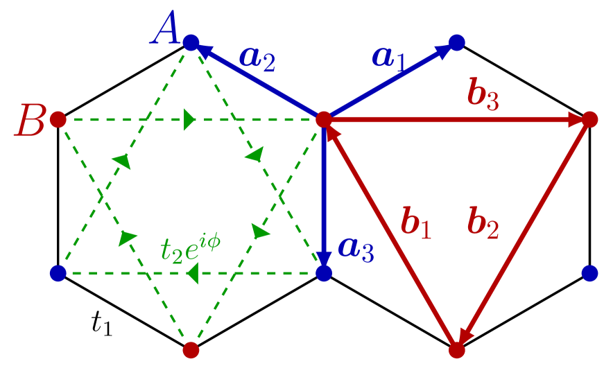
(a)

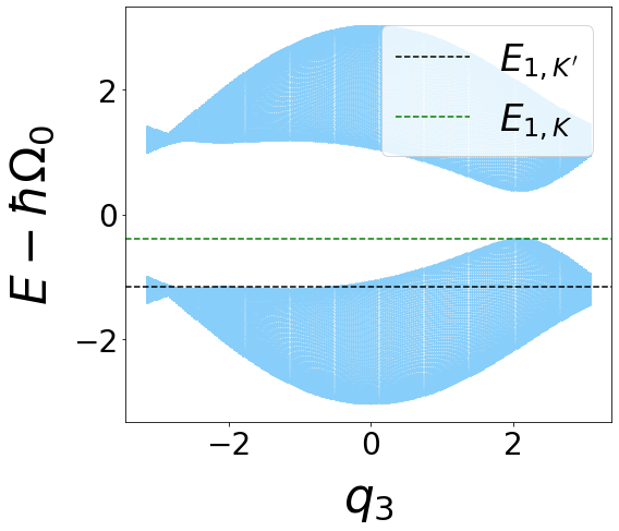
(b)

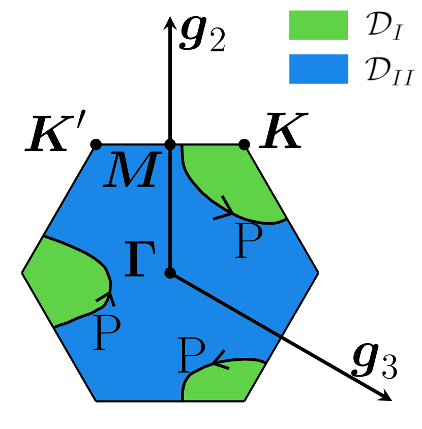
(c)

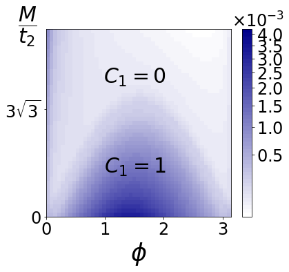
(d)

Figure 1: (a) Definition of the sublattices, real space vectors and hopping amplitudes for the Haldane model on the honeycomb lattice. (b) Haldane model energies, in units of $t_{1}$, as a function of the momentum $q_{3}=a{\bf k}\cdot{\bf g}_{3}$ ($a$ is the lattice spacing), with parameters $\phi=\pi/2$, $t_{2}=0.15t_{1}$ and $M=3\sqrt{3}t_{2}/2$. Both lowest band energies at the Dirac points, $E_{1,{\bf K}}$ and $E_{1,{\bf K}^{\prime}}$, are shown. (c) Brillouin zone for the honeycomb lattice and the $\mathcal{D}_{I}$ and $\mathcal{D}_{II}$ domains. (d) The quantity $1-\int d\omega S^{\textrm{out}}(\omega)$, computed from Eq. (9); the color scale of the figure is logarithmic. We considered $\textrm{sgn}\,M=\textrm{sgn}\left(\sin\phi\right)=1$, $j_{0}=1$, and the energies $\Omega_{0}=10$ GHz, $t_{1}/\hbar=100$ MHz, $t_{2}=0.15t_{1}$, $\Delta_{\textrm{CI}}=\Delta_{\textrm{P}}=10$MHz and $g_{q_{0}}/\hbar=1$MHz, as described in the main text. We considered a $30\times 30$ unit cells Haldane model with periodic boundary conditions.

Topological properties.—

Following the approach of Kohmoto [51], we will write the Chern number $C_{i}$ (energy band $i=1$ or $i=2$) in terms of a phase entering in the wavefunction, which is associated to the definition of the $h_{1}({\bf k})$ kinetic term only. This will elegantly allow us to show that the light probe can detect the topological response of the system locally within the Brillouin zone through the conservation of energy.

Table 1: Sign of $h_{2}$ at the Dirac points, as a function of $M$ and $\textrm{sgn}(\sin\phi)$.

	$|M|<3\sqrt{3}t_{2}|\sin\phi|$	$|M|>3\sqrt{3}t_{2}|\sin\phi|$
$\textrm{sgn}\,h_{2}({\bf K})$	$-\textrm{sgn}(\sin\phi)$	$\textrm{sgn}\,M$
$\textrm{sgn}\,h_{2}({\bf K}^{\prime})$	$\textrm{sgn}(\sin\phi)$	$\textrm{sgn}\,M$

We write $\ket{u_{i,{\bf k}}}$ the Bloch eigenvectors of the Haldane Hamiltonian, i.e. $\textrm{e}^{-i{\bf k}\cdot\hat{{\bf r}}}H\textrm{e}^{i{\bf k}\cdot\hat{{\bf r}}}\ket{u_{i,{\bf k}}}=E_{i,{\bf k}}\ket{u_{i,{\bf k}}}$ and we define the coefficients $\alpha_{i}^{1}({\bf k})$ and $\alpha_{i}^{2}({\bf k})$ such that $\ket{u_{i,{\bf k}}}=\left[\alpha_{i}^{1}({\bf k})a_{1,{\bf k}}^{\dagger}+\alpha_{i}^{2}({\bf k})a_{2,{\bf k}}^{\dagger}\right]\ket{0}$. These coefficients may vanish only at the Dirac points.

(i) If the sign of $h_{2}$ is opposite at the Dirac points ($|M|<3\sqrt{3}t_{2}|\sin\phi|$, see Table 1), then $\alpha_{i}^{1}({\bf k})$ and $\alpha_{i}^{2}({\bf k})$ vanish at the opposite Dirac points. It follows that it is impossible to find a unique and smooth phase over all the BZ for the Bloch state $\ket{u_{i,{\bf k}}}$. Rather, we choose to define two non-overlapping domains $\mathcal{D}_{I}$ and $\mathcal{D}_{II}$ in the BZ, each containing a different Dirac point (see Fig. 1(c)), and we use a different gauge choice for the Bloch states in each domain [51]. We define a closed path P along the boundary between $\mathcal{D}_{I}$ and $\mathcal{D}_{II}$, surrounding once the Dirac points, and a smooth phase along P, $\varphi({\bf k})$, such that $\textrm{e}^{-i\varphi({\bf k})}=\left.\textrm{e}^{i{\bf k}\cdot{\bf a}_{3}}h_{1}({\bf k})^{*}\right/|h_{1}({\bf k})|$. Then $C_{i}$ reads

$$2\pi C_{i}=(-1)^{i}\,\textrm{sgn}(\sin\phi)\oint_{\textrm{P}}d{\bf k}\cdot{\bf\nabla}_{{\bf k}}\varphi({\bf k}).$$ (2)

From the expressions of $\varphi({\bf k})$ and $h_{1}({\bf k})$, we find that $\varphi({\bf k})$ changes by $-2\pi$ when moving along the entire closed path P. This gives $C_{i}=(-1)^{i+1}\,\textrm{sgn}(\sin\phi)$. Let us remark that the vanishing of Bloch eigenvectors’ components at different points in the BZ, which prevents the smooth definition of Bloch states, is a characteristic feature of Chern insulators. As we will see, this fundamental property forms the basis of the probe proposed in this letter, rendering it a priori relevant for all Chern insulators.

(ii) If the sign of $h_{2}$ is the same at both Dirac points ($|M|>3\sqrt{3}t_{2}|\sin\phi|$, see Table 1), then $\alpha_{i}^{1}({\bf k})$ or $\alpha_{i}^{2}({\bf k})$ can be chosen non-zero over all the BZ, and it is possible to find a unique and smooth phase for $\ket{u_{i,{\bf k}}}$, leading to a unique and smooth Berry gauge field. Because the BZ is a torus, we find that the Chern numbers $C_{i}$ are vanishing.

From this analysis, for $|M|\neq 3\sqrt{3}t_{2}|\sin\phi|$, we find $C_{i}=(-1)^{i+1}\,\textrm{sgn}(\sin\phi)\left[1-\textrm{sgn}(h_{2}({\bf K})h_{2}({\bf K}^{\prime})\right]/2$, i.e.

$$C_{i}=\dfrac{(-1)^{i}}{2}\left[\textrm{sgn}\,h_{2}({\bf K})-\textrm{sgn}\,h_{2}({\bf K}^{\prime})\right].$$ (3)

This formula has in fact a simple physical understanding for a Hamiltonian $h_{\bf k}$ written as a $2\times 2$ matrix. From the Ehrenfest theorem and a Bloch sphere correspondence the topological number is equivalent to $C_{i}=(-1)^{i}\left[\langle\sigma_{z}(0)\rangle-\langle\sigma_{z}(\pi)\rangle\right]/2$ with $\langle\sigma_{z}\rangle=(-1)^{i}\cos\theta=(-1)^{i}\hbox{sgn}\,h_{2}(\theta)$ [53]. In the following, we namely rely on Eq. (3) to show how $C_{i}$ can be probed from the reflected light in a local probe capacitively coupled to a Haldane photonic system. The simple idea behind our proposal is that the topological properties manifest as discernible sublattice weight variations of the wave function, enabling to reveal the topological transition through the coupling of a probe to one of the sublattice sites.

Spectroscopic probe.—

Let us consider a local light probe with weak capacitive coupling to a Haldane boson model. The probe is a resonator with a certain number of (relevant) modes, each mode $q$ being characterized by the frequency $\omega_{q}$. The probe is coupled to the system at position ${\bf R}_{0}$, on the sublattice identified by the index $j_{0}$, where $j_{0}=1$ ($j_{0}=2$) for the sublattice A (B). We write the Hamiltonian associated to the probe $H_{\textrm{prb}}=\sum_{q}\hbar\omega_{q}b_{q}^{\dagger}b_{q}$, with $b_{q}$ the annihilation operators for the mode $q$ of the probe. The coupling is described by $H_{\textrm{cpl}}=\left(a_{{\bf R}_{0}}+a_{{\bf R}_{0}}^{\dagger}\right)\sum_{q}g_{q}\left(b_{q}+b_{q}^{\dagger}\right)$, with $a_{{\bf R}_{0}}^{\dagger}$ the creation operator for a boson at site ${\bf R}_{0}$. For simplicity, first of all, we disregard the dissipation effects induced by the probe in the Chern insulator and we assume that the light modes $\ket{u_{i,{\bf k}}}$ exhibit an infinitely long lifetime.

Table 2: Coefficients $\alpha_{i}^{j_{0}}$ which, at the Dirac points, are directly related to the Chern number, as a function of $\textrm{sgn}\,M$ and $\textrm{sgn}(\sin\phi)$.

	$\textrm{sgn}\,M=\textrm{sgn}\left(\sin\phi\right)$	$\textrm{sgn}\,M=-\textrm{sgn}\left(\sin\phi\right)$
$\textrm{sgn}\left(\sin\phi\right)=(-1)^{i}$	$\alpha_{i}^{2}(\bm{K})=-C_{i}$	$\alpha_{i}^{1}(\bm{K}^{\prime})=(-1)^{i+1}C_{i}$
$\textrm{sgn}\left(\sin\phi\right)=(-1)^{i+1}$	$\alpha_{i}^{1}(\bm{K})=(-1)^{i}C_{i}$	$\alpha_{i}^{2}(\bm{K}^{\prime})=C_{i}$

Table 3: Choice of the probe’s input frequency $\hbar\omega_{q_{0}}=E_{i,{\bf k}}$, given by the indices $i$ and ${\bf k}$, as a function of $\textrm{sgn}\,M$ and $\textrm{sgn}\left(\sin\phi\right)$, such that the transition rate depends on the Chern number: $\Gamma=J\left[E_{i,{\bf k}}\right]|C_{i}|/\hbar$.

	$\textrm{sgn}\,M=\textrm{sgn}\left(\sin\phi\right)$	$\textrm{sgn}\,M=-\textrm{sgn}\left(\sin\phi\right)$
$\textrm{sgn}\left(\sin\phi\right)=1$	$i=j_{0}$, ${\bf k}={\bf K}$	$i=\overline{j_{0}}$, ${\bf k}={\bf K}^{\prime}$
$\textrm{sgn}\left(\sin\phi\right)=-1$	$i=\overline{j_{0}}$, ${\bf k}={\bf K}$	$i=j_{0}$, ${\bf k}={\bf K}^{\prime}$

To build intuition, let us show that the transition rate $\Gamma$ from a state $\ket{\psi(t)}$ which, at initial time $t_{i}$, is a probe’s mode with frequency $\omega_{q_{0}}$, i.e. $\ket{\psi(t_{i})}=\ket{b_{q_{0}}}$, to the eigenstates $\ket{u_{i,{\bf k}}}$ of the Haldane Hamiltonian’s bears information about the topological character of the system. Fermi Golden rule states that at sufficiently long times $t$, $\Gamma\left[\hbar\omega_{q_{0}}\right]=\dfrac{2\pi}{\hbar}\sum_{i,{\bf k}}|\bra{b_{{q_{0}}}}H_{\textrm{cpl}}\ket{u_{i,{\bf k}}}|^{2}\delta\left(\hbar\omega_{q_{0}}-E_{i,{\bf k}}\right)$. $\bra{b_{{q_{0}}}}H_{\textrm{cpl}}\ket{u_{i,{\bf k}}}$ involves the components of the Bloch state in the basis $\left(a_{1,{\bf k}}^{\dagger},a_{2,{\bf k}}^{\dagger}\right)$ and a factor $\textrm{e}^{i{\bf k}\cdot{\bf R}_{0}}$ (transformation to the real space representation), such that we obtain $\bra{b_{{q_{0}}}}H_{\textrm{cpl}}\ket{u_{i,{\bf k}}}=g_{q_{0}}\alpha_{i}^{j_{0}}({\bf k})\textrm{e}^{i{\bf k}\cdot{\bf R}_{0}}$. As one can see from Table 2, which is constructed using Eq. (3) and the related analysis of the coefficients $\alpha_{i}^{j_{0}}({\bf k})$, depending on $\textrm{sgn}\,M$ and $\textrm{sgn}\left(\sin\phi\right)$, it is possible to express the Chern number as a function of the coefficients $\alpha_{i}^{j_{0}}({\bf k})$. If $\textrm{sgn}\,M=\textrm{sgn}\left(\sin\phi\right)$ ($\textrm{sgn}\,M=-\textrm{sgn}\left(\sin\phi\right)$) we notice that the Chern number is directly related to the coefficients $\alpha_{i}^{j_{0}}({\bf k})$ evaluated at $\bm{K}$ ($\bm{K}^{\prime}$) and $E_{i,\bm{K}}$ ($E_{i,\bm{K}^{\prime}}$), $i\in\{1,2\}$, is non-degenerate. Therefore, choosing $\hbar\omega_{q_{0}}=E_{i,{\bf k}}$ with $i$ and ${\bf k}$ according to Table 3, we find a simple relation between $\Gamma$ and the topological invariant: $\Gamma\left[E_{i,{\bf k}}\right]=J\left[E_{i,{\bf k}}\right]|C_{i}|^{2}=J\left[E_{i,{\bf k}}\right]|C_{i}|$, where the spectral function $J$ is: $J[\omega]=(2\pi/\hbar)\sum_{q}g_{q}^{2}\left[\delta(\omega-\omega_{q})-\delta(\omega+\omega_{q})\right]$. In other words,

$$\Gamma\left[E_{i,{\bf k}}\right]=J\left[E_{i,{\bf k}}\right]|C_{i}|,$$ (4)

where the indices $i$ and ${\bf k}$ are functions of $\textrm{sgn}\,M$ and $\textrm{sgn}\left(\sin\phi\right)$ as indicated in Table 3. The relation appearing in Eq. (4) has been established from Table 2 and Table 3, which are constructed from the previous section. Therefore, Eq. (4) relies on a fundamental property characterizing a Chern insulator: the impossibility of defining smooth Bloch states over the BZ, which translates here into the vanishing of the Bloch eigenvectors’ components $\alpha_{i}^{1}$ and $\alpha_{i}^{2}$ at the opposite Dirac points.

Motivated by this, we now investigate the relation between an input voltage $\langle V_{{\bf R}_{0}}^{\textrm{in}}[\omega]\rangle$ and the resulting output voltage $\langle V_{{\bf R}_{0}}^{\textrm{out}}[\omega]\rangle$, both at frequency $\omega$ in the probe at ${\bf R}_{0}$. For $\omega$ resolved around one Dirac point, this relation between $\langle V_{{\bf R}_{0}}^{\textrm{in}}[\omega]\rangle$ and $\langle V_{{\bf R}_{0}}^{\textrm{out}}[\omega]\rangle$ enables to rebuild the Haldane topological phase diagram . To fourth order in the coupling amplitudes $\{g_{q}\}$, we indeed find

$$\langle V_{{\bf R}_{0}}^{\textrm{out}}[\omega]\rangle=R(\omega)\langle V_{{\bf R}_{0}}^{\textrm{in}}[\omega]\rangle,$$ (5)

with $R(\omega)=1+iJ[\omega]\chi_{{\bf R}_{0},{\bf R}_{0}}$, and

$$\chi_{{\bf R}_{0},{\bf R}_{0}}=\dfrac{1}{N}\sum_{i=1}^{2}\sum_{{\bf k}}\gamma_{j_{0},{\bf k}}^{i}\left[\dfrac{1}{-\hbar\omega-E_{i,{\bf k}}+i0^{+}}-\dfrac{1}{-\hbar\omega+E_{i,{\bf k}}+i0^{+}}\right],$$ (6)

where $N$ is the number of lattice sites and

$$\gamma_{j_{0},{\bf k}}^{i}=\dfrac{1}{2}+\dfrac{(-1)^{j_{0}+i+1}h_{2}({\bf k})}{2\epsilon({\bf k})}\in\,\mathbb{R}.$$ (7)

From $\epsilon({\bf k})=\sqrt{|h_{1}({\bf k})|^{2}+h_{2}({\bf k})^{2}}$, we notice that $\gamma_{j_{0},{\bf k}}^{i}$ evaluated at the Dirac points depends on the sign of the function $h_{2}$: we have $2\gamma_{j_{0},{\bf k}}^{i}=1-(-1)^{j_{0}+i}\textrm{sgn}\,h_{2}({\bf k})$ for ${\bf k}=\{{\bf K},{\bf K}^{\prime}\}$. This is related to the topological invariant via the Eq. (3) and Table 1. As we show in Table 4, depending on the sign of $\sin\phi$ and on the sign of the Semenoff mass, the $i^{\textrm{th}}$ band topological invariant is given by the coefficient $\gamma_{j_{0},{\bf k}}^{i}$, evaluated at $j_{0}=i$ or $j_{0}=\overline{i}$ and at ${\bf k}={\bf K}$ or ${\bf k}={\bf K}^{\prime}$, with $\overline{i}=2(1)$ if $i=1(2)$. Again, this outcome is obtained thanks to a fundamental characteristic associated to the topological phase: the vanishing of the Bloch eigenvectors’ components $\alpha_{i}^{1}$ and $\alpha_{i}^{2}$ at the opposite Dirac points.

Table 4: Value of $\gamma_{j_{0},{\bf k}}^{i}$, evaluated at $j_{0}=i$ or $j_{0}=\overline{i}$ and at ${\bf k}={\bf K}$ or ${\bf k}={\bf K}^{\prime}$, as a function of $\textrm{sgn}\left(\sin\phi\right)$ and $\textrm{sgn}\,M$. We remind that $\overline{i}=2(1)$ if $i=1(2)$.

	$\textrm{sgn}\,M=\textrm{sgn}\left(\sin\phi\right)$	$\textrm{sgn}\,M=-\textrm{sgn}\left(\sin\phi\right)$
$\textrm{sgn}\left(\sin\phi\right)=1$	$\gamma_{i,\bm{K}}^{i}=(-1)^{\overline{i}}C_{i}$	$\gamma_{\overline{i},\bm{K}^{\prime}}^{i}=(-1)^{\overline{i}}C_{i}$
$\textrm{sgn}\left(\sin\phi\right)=-1$	$\gamma_{\overline{i},\bm{K}}^{i}=(-1)^{i}C_{i}$	$\gamma_{i,\bm{K}^{\prime}}^{i}=(-1)^{i}C_{i}$

Now, we can understand how a simple measurement of the reflection of a light input in the probe gives access to the topological invariant. We write $S^{\textrm{in}}(\omega)=\left|\langle V_{{\bf R}_{0}}^{\textrm{in}}[\omega]\rangle\right|^{2}$ and $S^{\textrm{out}}(\omega)=\left|\langle V_{{\bf R}_{0}}^{\textrm{out}}[\omega]\rangle\right|^{2}$ the energy spectral density respectively associated to the input and output voltages. To leading order in the coupling amplitudes, we have $S^{\textrm{out}}(\omega)=|R(\omega)|^{2}S^{\textrm{in}}(\omega)$ and for $\omega>0$,

$$|R(\pm\omega)|^{2}=1\mp\dfrac{2\pi J[\pm\omega]}{N}\sum_{i=1}^{2}\sum_{{\bf k}}\gamma_{j_{0},{\bf k}}^{i}\delta(\hbar\omega-E_{i,{\bf k}}).$$ (8)

For $\textrm{sgn}\,M=\textrm{sgn}\left(\sin\phi\right)$, the energies $E_{i,\bm{K}},\,i\in\{1,2\}$ are non-degenerate, therefore, choosing $\hbar\omega=E_{i,\bm{K}}$ selects only the ${\bf k}={\bf K}$ point in the integral appearing in the Eq. (8). Moreover, as indicated in Table 4, $\gamma_{j_{0},{\bf K}}^{i}$ is related to the topological invariant if we choose a probe at $j_{0}=i$ ($\overline{i}$) for $\textrm{sgn}\left(\sin\phi\right)=1$ ($\textrm{sgn}\left(\sin\phi\right)=-1$). Therefore, for a well-chosen frequency $\omega$, $|R(\omega)|^{2}$ clearly depends on the topological invariant. This is also true for $\textrm{sgn}\,M=-\textrm{sgn}\left(\sin\phi\right)$, if, in the previous analysis, we replace ${\bf K}$ by ${\bf K}^{\prime}$ and $j_{0}$ by $\overline{j_{0}}$.

Finite lifetimes for the light modes.—

Eventually, we address the more realistic scenario in which we incorporate finite lifetimes for both the modes in the probe $\ket{b_{q}}$ and the Chern insulator’s modes $\ket{u_{i,{\bf k}}}$. For simplicity, we consider the same bandwidth amplitude $\Delta_{\textrm{CI}}$ ($\Delta_{\textrm{P}}$) for all the modes $\ket{u_{i,{\bf k}}}$ ($\ket{b_{q}}$). We assume the following ordering of the energies $\textrm{max}_{q}(g_{q})\ll\{\Delta_{\textrm{CI}},\Delta_{\textrm{P}}\}\ll\{t_{1},\textrm{min}_{q,q^{\prime}}(|\omega_{q}-\omega_{q^{\prime}}|)\}$. We replace the Dirac Delta functions appearing in Eq. (8) by normalized Gaussian spectral distributions denoted $G\left(\omega;\overline{\omega},\Delta\right)$ with mean value $\overline{\omega}$ and standard deviation $\Delta$: $\delta(\hbar\omega-E_{i,{\bf k}})$ is replaced by $G\left(\omega;E_{i,{\bf k}}/\hbar,\Delta_{\textrm{CI}}\right)$ and $J[\omega]$ is replaced by $\tilde{J}[\omega]=2\pi\sum_{q}\left(g_{q}/\hbar\right)^{2}\left[G\left(\omega,\omega_{q},\Delta_{\textrm{P}}\right)-G\left(\omega,-\omega_{q},\Delta_{\textrm{P}}\right)\right]$. We also consider an input energy spectral density with Gaussian distribution: $S^{\textrm{in}}(\omega)=G\left(\omega;\omega_{q_{0}},\Delta_{\textrm{P}}\right)$. For a well chosen $\omega_{q_{0}}$ ($E_{i,\bm{K}}$ or $E_{i,\bm{K}}$), $|R(\omega)|^{2}$ still depends on the topological invariant because $\gamma_{j_{0},{\bf k}}^{i}$ is directly related to the Chern number. To illustrate this point, let us consider the case $\textrm{sgn}\,M=\textrm{sgn}\left(\sin\phi\right)=1$ for which we choose $\hbar\omega_{q_{0}}=E_{1,\bm{K}}$ and $j_{0}=i=1$ and we expect $\gamma_{1,{\bf K}}^{1}=C_{1}$. $S^{\textrm{out}}(\omega)$ depends on $\gamma_{1,{\bf K}}^{1}$, especially around $\omega=\omega_{q_{0}}$, leading to a decrease of the output peak’s weight $\int d\omega S^{\textrm{out}}(\omega)$ compared to the normalized weight of the input peak. This decrease is given by

$$1-\int d\omega S^{\textrm{out}}(\omega)=\dfrac{2\pi}{N}\sum_{i=1}^{2}\sum_{{\bf k}}\gamma_{j_{0},{\bf k}}^{i}I_{i,{\bf k}},$$ (9)

with $I_{i,{\bf k}}=\int d\omega\tilde{J}[\omega]G\left(\omega;E_{i,{\bf k}}/\hbar,\Delta_{\textrm{CI}}\right)G\left(\omega;E_{1,{\bf K}}/\hbar,\Delta_{\textrm{P}}\right)$, which is $\left(g_{q_{0}}/\hbar\right)^{2}/\left(\sqrt{2\pi}\Delta_{\textrm{CI}}\Delta_{\textrm{P}}^{2}\right)$ times the overlap area $\int d\omega\,\textrm{exp}{-\dfrac{\left(\omega-E_{1,{\bf K}}/\hbar\right)^{2}}{\Delta_{\textrm{P}}^{2}}}\,\textrm{exp}{-\dfrac{\left(\omega-E_{i,{\bf k}}/\hbar\right)^{2}}{2\Delta_{\textrm{CI}}^{2}}}$ . $1-\int d\omega S^{\textrm{out}}(\omega)$ reproduces the topological phase diagram associated to the Haldane model, as we show in Fig. 1(d), from a numerical evaluation of Eq. (9), with the energy scales $\Omega_{0}=10$ GHz, $t_{1}/\hbar=100$ MHz, $\Delta_{\textrm{CI}}=\Delta_{\textrm{P}}=10$MHz and $g_{q_{0}}/\hbar=1$MHz. These scales corresponds to a relatively low quality factor $Q=\Omega_{0}/\Delta_{\textrm{CI}}=10^{3}$ (here the same for both the cQED Chern insulator and the probe) and a low coupling amplitude and should be reachable in a cQED experiment.

Magnon system and material suggestions.—

The results described here are directly relevant for other Chern insulator systems. For instance, our probe can be used for a topological magnon insulator, as the one proposed in Ref. [55], which is described by a bosonic Haldane model. Indeed, consider a magnetic tip described by a polarization state denoted ${\bf s}=(s^{x},s^{y},s^{z})$, and assume the tip thin enough to couple to only one magnetic site ${\bf S}_{i}$ of the system. The Hamiltonian coupling the tip to the magnon system is $H_{\textrm{cpl}}=J\,{\bf S}_{i}\cdot{\bf s}_{i}$, with $J$ the coupling amplitude. Suppose now the tip is polarized along $x$ only. Then $H_{\textrm{cpl}}=J\,{\bf S}_{i}\cdot{\bf s}_{i}=(J/4)(S_{i}^{+}+S_{i}^{-})(s^{+}+s^{-})$, where $S_{i}^{+}$, $S_{i}^{-}$, $s^{+}$ and $s^{-}$ are bosonic creation/annihilation operators. $H_{\textrm{cpl}}$ is completely analogue to the coupling Hamiltonian we considered for the cQED system. Therefore, measuring the response to a magnetic excitation provides a way to access the topological number. Such a measurement should be applicable in topological magnon quantum materials, such as CrI₃ [56] or maybe $\beta$-Cu₂V₂O₇ [57]. Even though the magnon can condense at the lowest energy mode, thermal excitation shall generate magnon modes at all energies in the system, namely the ones required for the proposed probe, with energy around the Dirac point.

Remarks.—

Several observations are in order.

(i) Topological insulators are robust against weak disorder. Then we expect the general structure of the wave function over space, which is related to the bulk invariant, to be robust against disorder. This central feature give robustness to the probe proposed in this letter. In a magnon system, even though the disorder could be high compared to cQED systems, a magnetic tip enables to scan several sites in the sample; averaging the output signal over these sites would mitigate disorder effects.

(ii) It is interesting to observe that the probe is able to measure the topological number based on a real space local coupling to the system and with a resolution in reciprocal space thanks to the energy conservation, similarly to circularly polarized light [28].

(iii) We checked the applicability of the probe proposed here to a simple topological bosonic kagome system.

(iv) From Eqs. (7) and (8), we notice that the energy density of states at $\hbar\omega=E_{i,\bm{k}}$ can be evaluated by summing the local responses $1-\textrm{Re}\left[R(\omega)\right]$ measured separately in a probe at $j_{0}=1$ (sublattice A) and in a probe at $j_{0}=2$ (sublattice B).

(v) If the input is triggered at a site with position ${\bf r}$ lying on the sublattice $j_{0}$ and the output is measured at a different site with position ${\bf r}^{\prime}$ and sublattice index $j_{0}^{\prime}$ , the expression in the summation of Eq. (6) is replaced by

$$\dfrac{\left[\beta_{j_{0}}^{i}({\bf k})\alpha_{i}^{j_{0}^{\prime}}({\bf k})\right]^{*}\textrm{e}^{i{\bf k}\left({\bf r}-{\bf r}^{\prime}\right)}}{-\hbar\omega-E_{i,{\bf k}}+i0^{+}}-\dfrac{\beta_{j_{0}}^{i}({\bf k})\alpha_{i}^{j_{0}^{\prime}}({\bf k})\textrm{e}^{-i{\bf k}\left({\bf r}-{\bf r}^{\prime}\right)}}{-\hbar\omega+E_{i,{\bf k}}+i0^{+}},$$ (10)

with $\beta_{j_{0}}^{i}({\bf k})\alpha_{i}^{j_{0}}({\bf k})=\gamma_{j_{0},{\bf k}}^{i}$ and for $j_{0}^{\prime}=\overline{j_{0}}\neq j_{0}$, $\beta_{j_{0}}^{i}({\bf k})\alpha_{i}^{\overline{j_{0}}}({\bf k})\propto h_{1}({\bf k})/2\epsilon({\bf k})$. At the Dirac points, $h_{1}$ is vanishing, therefore, in the case $j_{0}^{\prime}=\overline{j_{0}}$, the simple protocol we sketched above does not help to rebuild the topological phase diagram. This outcome can be anticipated based on the fact that, at one given Dirac point, one of both Bloch eigenvectors’ components vanish, in the topological regime. In the scenario $j_{0}^{\prime}=j_{0}$, because the coefficients in the numerator of Eq. (10) are complex-valued, the Chern number dependency of $1-\int d\omega S^{\textrm{out}}(\omega)$ is mitigated. Indeed, the latter contains principal values of integrals over frequency involving $\left[1/\left(-\hbar\omega\pm E_{i,{\bf k}}\right)\right]$ terms.

Conclusion.—

We have considered a local microwave-light probe with capacitive coupling to a cQED array described by a Haldane bosonic system, in the regime of small coupling amplitudes. We have explained how this probe is relevant for the detection of the topological character of Chern insulators. Firstly, using FGR, we established a connection between the Chern number and the transition rate from a probe’s eigenstate (with frequency corresponding to one of the Dirac points energy) to the eigenstates of the Haldane Hamiltonian. Secondly, we developed the input-output theory for the probe, enabling us to compute the reflection coefficient which relates an input voltage and an output voltage. We showed that for an input with frequency resolved at one of the Dirac points, this reflection coefficient is directly related to the system’s topological invariant. The fundamental working principle of this probe makes it inherently relevant for all Chern insulators. Additionally, as a future prospect, it appears both possible and intriguing to adapt this probe to other systems that may exhibit different particle statistics, such as cold atoms or various material platforms.

Acknowledgments.—

This work was supported by the french ANR BOCA grant. JL acknowledges support from the National Research Fund Luxembourg under Grant No. INTER/QUANTERA21/16447820/MAGMA.

Supplemental Material

In this Supplemental Material, we show, in Sec. S1, the details of the Chern number’s computation used in the main text, in relation with the Bloch eigenvectors’ components properties over the BZ. In Sec. S2, we show the computation of the coefficient which relates input voltages in a set of probes capacitively coupled to a bosonic lattice model and the resulting output voltage in a one of these probes.

S1 Chern number, gauge choices and unique and smooth Berry gauge fields

In this section we show a detailed analytical computation of the Chern number, based on an approach introduced by Kohmoto [51], for the Haldane system with Hamiltonian defined in the Eq. (1). This computation relies on the definition of two distinct gauge choices $G_{I}$ and $G_{II}$ for the Bloch eigenvectors $\ket{u_{i,{\bf k}}}=\left[\alpha_{i}^{1}({\bf k})a_{1,{\bf k}}^{\dagger}+\alpha_{i}^{2}({\bf k})a_{2,{\bf k}}^{\dagger}\right]\ket{0}\,,$ that we respectively write $\ket{u_{i,{\bf k},I}}$ and $\ket{u_{i,{\bf k},II}}$.

(i) Gauge choice $G_{I}$: the coefficient $\alpha_{i}^{1}({\bf k})$ is real. More precisely, we choose

$$\alpha_{i}^{1}({\bf k})=\rho_{i}({\bf k})\,,$$ (S1)

with

$$\rho_{i}({\bf k})=\dfrac{h_{2}({\bf k})+(-1)^{i}\epsilon({\bf k})}{2\left[\epsilon({\bf k})^{2}+(-1)^{i}h_{2}({\bf k})\epsilon({\bf k})\right]^{1/2}},$$ (S2)

and we have

$$\alpha_{i}^{2}({\bf k})=\lambda_{i}({\bf k})\textrm{e}^{-i\varphi({\bf k})}\,,$$ (S3)

with

$$\lambda_{i}({\bf k})=\dfrac{|h_{1}({\bf k})|}{2\left[\epsilon({\bf k})^{2}+(-1)^{i}h_{2}({\bf k})\epsilon({\bf k})\right]^{1/2}},$$ (S4)

and

$$\textrm{e}^{-i\varphi({\bf k})}=\dfrac{\textrm{e}^{i{\bf k}\cdot{\bf a}_{3}}h_{1}({\bf k})^{*}}{|h_{1}({\bf k})|}.$$ (S5)

(ii) Gauge choice $G_{II}$: the coefficient $\alpha_{i}^{2}({\bf k})$ is real. We choose $\ket{u_{j,{\bf k},II}}=\textrm{e}^{i\varphi({\bf k})}\ket{u_{j,{\bf k},I}}$, i.e.

$$\alpha_{i}^{2}({\bf k})=\lambda_{i}({\bf k}),$$ (S6)

and we have

$$\alpha_{i}^{1}({\bf k})=\rho_{i}({\bf k})\textrm{e}^{i\varphi({\bf k})}.$$ (S7)

Table SI: Table giving the values of of $\rho_{i}({\bf k})$ and $\lambda_{i}({\bf k})$ at the Dirac points in the case $|M|<3\sqrt{3}t_{2}|\sin\phi|$ , as a function of the sign of the Semenoff mass $M$ and of the index of the energy band $i$.

	$\textrm{sgn}(\sin\phi)=(-1)^{i}\,$	$\textrm{sgn}(\sin\phi)=(-1)^{i+1}\,$
$\rho_{i}({\bf k}\rightarrow{\bf K})$	$0$	$(-1)^{i}$
$\rho_{i}({\bf k}\rightarrow{\bf K}^{\prime})$	$(-1)^{i}$	$0$
$\lambda_{i}({\bf k}\rightarrow{\bf K})$	$1$	$0$
$\lambda_{i}({\bf k}\rightarrow{\bf K}^{\prime})$	$0$	$1$

Table SII: Table giving the values of of $\rho_{i}({\bf k})$ and $\lambda_{i}({\bf k})$ at the Dirac points in the case $|M|>3\sqrt{3}t_{2}|\sin\phi|$, as a function of the sign of the Semenoff mass $M$ and of the index of the energy band $i$.

	$\textrm{sgn}\,M=(-1)^{i}\,$	$\textrm{sgn}\,M=(-1)^{i+1}\,$
$\rho_{i}({\bf k}\rightarrow{\bf K})$	$(-1)^{i}$	$0$
$\rho_{i}({\bf k}\rightarrow{\bf K}^{\prime})$	$(-1)^{i}$	$0$
$\lambda_{i}({\bf k}\rightarrow{\bf K})$	$0$	$1$
$\lambda_{i}({\bf k}\rightarrow{\bf K}^{\prime})$	$0$	$1$

The phase of the wavefunction is chosen by requiring that either the coefficient $\alpha_{i}^{1}({\bf k})$ or the coefficient $\alpha_{i}^{2}({\bf k})$ is real (and non-zero). $\rho_{i}({\bf k})$ and $\lambda_{i}({\bf k})$ may vanish only at the Dirac points and it depends on the sign of $h_{2}$, given in Table 1 as a function of $M$ and $\phi$. For $|M|<3\sqrt{3}t_{2}|\sin\phi|$ ($|M|>3\sqrt{3}t_{2}|\sin\phi|$), the values of $\rho_{i}({\bf k})$ and $\lambda_{i}({\bf k})$ at the Dirac points are given in Table SI (Table SII).

(i) In the case $|M|<3\sqrt{3}t_{2}|\sin\phi|$, we notice that (see Table SI), for all the values of $\phi$, none of both gauge choices $G_{I}$ and $G_{II}$ is well-defined in the entire BZ. Indeed, $\rho_{i}({\bf k})$ and $\lambda_{i}({\bf k})$ each vanish at one of the Dirac points. As explained in the main text, we then define two non-overlapping domains in the BZ [51] and use a different gauge choice in each domain. To be more specific, for $(-1)^{i}\,\textrm{sgn}(\sin\phi)=+1$, we apply $G_{I}$ for the points contained in $\mathcal{D}_{II}$ and $G_{II}$ for the points contained in $\mathcal{D}_{I}$ while for $(-1)^{i}\,\textrm{sgn}(\sin\phi)=-1$, we apply $G_{I}$ for the points contained in $\mathcal{D}_{I}$ and $G_{II}$ for the points contained in $\mathcal{D}_{II}$. Then the phase of $\ket{u_{i,{\bf k},I}}$ (the eigenstate in $\mathcal{D}_{I}$) and $\ket{u_{i,{\bf k},II}}$ (the eigenstate in $\mathcal{D}_{II}$) and the Berry gauge fields ${\bf A}_{i,{\bf k},I}=\bra{u_{i,{\bf k},I}}{\bf\nabla}_{{\bf k}}\ket{u_{i,{\bf k},I}}$ and ${\bf A}_{i,{\bf k},II}=\bra{u_{i,{\bf k},II}}{\bf\nabla}_{{\bf k}}\ket{u_{i,{\bf k},II}}$ are uniquely and smoothly defined respectively on $\mathcal{D}_{I}$ and $\mathcal{D}_{II}$. The Chern number associated to the $j^{\textrm{th}}$ band (remind that $j=1$ or $j=2$) reads

$$C_{j}=\dfrac{1}{2i\pi}\bigg{[}\int_{\mathcal{D}_{\textrm{I}}}d^{2}k\left({\bf\nabla}_{{\bf k}}\times{\bf A}_{j,{\bf k},\textrm{I}}\right)\cdot{\bf e}_{z}+\int_{\mathcal{D}_{\textrm{II}}}d^{2}k\left({\bf\nabla}_{{\bf k}}\times{\bf A}_{j,{\bf k},\textrm{II}}\right)\cdot{\bf e}_{z}\bigg{]}.$$ (S8)

Using Stokes’ theorem and considering the specific choice of path P shown in Fig. 1(c) leads to

$$C_{j}=\dfrac{1}{2i\pi}\left(\oint_{\textrm{P}}d{\bf k}\cdot{\bf A}_{j,{\bf k},\textrm{I}}-\oint_{\textrm{P}}d{\bf k}\cdot{\bf A}_{j,{\bf k},\textrm{II}}\right).$$ (S9)

Along P, we have $\ket{u_{j,{\bf k},I}}=\textrm{e}^{i(-1)^{j}\,\textrm{sgn}(\sin\phi)\varphi({\bf k})}\ket{u_{j,{\bf k},II}}$. We choose $\varphi({\bf k})$ so that it is smooth along the whole P path and we obtain

$$C_{j}=\dfrac{(-1)^{j}\,\textrm{sgn}(\sin\phi)}{2\pi}\oint_{\textrm{P}}d{\bf k}\cdot{\bf\nabla}_{{\bf k}}\varphi({\bf k}).$$ (S10)

$C_{i}$ is found by studying how $\varphi({\bf k})$ evolves when moving along P. Generally speaking, when the P path surround a $\varphi({\bf k})$’s divergence (here at the ${\bf K}$ or ${\bf K}^{\prime}$ point), the accumulated phase increases or decreases by $\pm 2\pi z,\,z\in\mathbb{Z}$, which gives a quantized value of $C$, as expected. Here, we find that $\varphi({\bf k})$ changes by $-2\pi$ when moving along the entire closed path P. One can build intuition from small displacement $\delta{\bf k}$ around $\bf K$, in which case we have $h_{1}({\bf K}+\delta{\bf k})=3t_{1}(-\delta k_{x}+i\delta k_{y})/2$ where $\delta k_{x}=\delta{\bf k}\cdot{\bf e}_{x}$, $\delta k_{y}=\delta{\bf k}\cdot{\bf e}_{y}$, ${\bf e}_{x}=-\left({\bf b}_{2}+{\bf b}_{3}\right)/\sqrt{3}$ and ${\bf e}_{y}=\left({\bf b}_{2}-{\bf b}_{3}\right)/3$. In this case, we easily see that $\varphi$, which is defined by $\textrm{e}^{-i\varphi({\bf k})}=\textrm{e}^{i{\bf k}\cdot{\bf a}_{3}}h_{1}({\bf k})^{*}/|h_{1}({\bf k})|$, varies by $-2\pi$, for one entire closed path P around $\bf K$ (oriented anticlockwise).

(iii) In the case $|M|>3\sqrt{3}t_{2}|\sin\phi|$, we gathered the values of $\rho_{i}({\bf k})$ and $\lambda_{i}({\bf k})$ at the Dirac points in Table SII. At both Dirac points, either $\rho_{i}({\bf k})$ or $\lambda_{i}({\bf k})$ are non-vanishing, therefore it is possible to find a unique and smooth phase for the ket $\ket{u_{i,{\bf k}}}$ everywhere in the BZ which leads to a unique and smooth Berry gauge field ${\bf A}_{{\bf k}}$. Depending on the value of $(-1)^{i}\,\textrm{sgn}(M)$, we apply gauge choice $G_{I}$ or $G_{II}$ for all the points of the BZ, and then we can show that the associated wave function $\ket{u_{i,{\bf k},I}}$ or $\ket{u_{i,{\bf k},II}}$ (and its phase) is uniquely and smoothly defined, as is the Berry gauge field.

S2 Local response to capacitively coupled probes in a two-dimensional lattice bosonic system

In this section, we consider a set of bosonic probes (typically microwave light resonators) capacitively coupled to a bosonic lattice model. We derive the relation between the output voltage operator in a probe at a certain position on the lattice and the input voltage operators associated to the ensemble of probes on the lattice. We consider a 2-dimensional lattice system with periodic boundary conditions.

S2.1 Hamiltonian

The Hamiltonian describing the lattice model with capacitively coupled probes reads

$$H=H_{\textrm{lat}}+H_{\textrm{prb}}+H_{\textrm{cpl}},$$ (S11)

where $H_{\textrm{lat}}$ is the (topological) lattice Hamiltonian, $H_{\textrm{prb}}$ is the Hamiltonian associated to the probe(s) and $H_{\textrm{cpl}}$ is the Hamiltonian associated to the coupling between the lattice and the probe(s).

Let us call $N_{C}$ the number of sites per unit cell in the lattice we consider and $N$ the total number of unit cells. We label each site within a unit cell with different colors, and two different sites belonging to the same Bravais lattice are labeled by the same color. We define the Fourier transform of the annihilation operator of a (bosonic) particle at position $\bf r$ and the inverse relation

$$a_{j,{\bf k}}=\sum_{{\bf r}\in R_{j}}\textrm{e}^{-i{\bf k}.{\bf r}}a_{{\bf r}}\quad\textrm{and}\quad a_{{\bf r}}=\dfrac{1}{N}\sum_{{\bf k}}\textrm{e}^{i{\bf k}.{\bf r}}a_{j({\bf r}),{\bf k}},$$ (S12)

with $R_{j}$ the ensemble containing all the lattice positions of the color-$j$ sites and the function $j({\bf r})$ returns the color index at the ${\bf r}$ site. We formally write

$$H_{\textrm{lat}}=\sum_{\bm{k}}\Psi_{\bm{k}}^{\dagger}h_{\bm{k}}\Psi_{\bm{k}},$$ (S13)

with $\Psi_{{\bf k}}^{\dagger}=\left(a_{1,{\bf k}}^{\dagger},\dots a_{N,{\bf k}}^{\dagger}\right)$. We write $h_{{\bf k}}$’s associated eigenvalues $E_{i,{\bf k}}$, where $i\in\{1,\dots,N_{C}\}$, and we write the associated eigenvectors

$$\ket{\Phi_{i,{\bf k}}}=\Phi_{i,{\bf k}}^{\dagger}\ket{0}=\sum_{j=1}^{N_{C}}\alpha_{i}^{j}({\bf k})a_{j,{\bf k}}^{\dagger}\ket{0},$$ (S14)

with $\alpha_{i}^{j}({\bf k})\in\mathbb{C}$. We have

$$H_{\textrm{lat}}=\sum_{{\bf k}}\sum_{i=1}^{N_{C}}E_{i,{\bf k}}\Phi_{i,{\bf k}}^{\dagger}\Phi_{i,{\bf k}}.$$ (S15)

Each probe are resonators with a certain number of relevant modes, each mode $q$ being characterized by the frequency $\omega_{q}$. Therefore we write

$$H_{\textrm{prb}}=\sum_{{\bf r}\in R_{p}}\sum_{q}\hbar\omega_{q}b_{\bm{r},q}^{\dagger}b_{{\bf r},q},$$ (S16)

with $b_{\bm{r},q}$ the annihilation operators for the mode $q$ of the probe at $\bm{r}\in R_{p}$, $R_{p}$ being the ensemble of the positions of the nodes coupled to a probe. We assume a capacitive coupling between each probe and a node of the lattice. The Hamiltonian reads

$$H_{\textrm{cpl}}=\sum_{{\bf r}\in R_{p}}\left(a_{\bf r}+a_{{\bf r}}^{\dagger}\right)\sum_{q}g_{q}\left(b_{{\bf r},q}+b_{{\bf r},q}^{\dagger}\right).$$ (S17)

The coupling amplitude $g_{q}$ is assumed not to depend on the position of the probe.

S2.2 Input-output analysis

Here we use the input-output formalism as reviewed in Ref. [58]. Let us define the input voltage in the probe at $\bf r$

$$V_{\bf r}^{\textrm{in}}(t)=\sum_{q}g_{q}\left[\textrm{e}^{-i\omega_{q}(t-t_{i})}b_{{\bf r},q}(t_{i})+h.c.\right],$$ (S18)

where $t_{i}<t$ is an initial time in the distant past, and the output voltage in the probe at $\bf r$

$$V_{\bf r}^{\textrm{out}}(t)=\sum_{q}g_{q}\left[\textrm{e}^{-i\omega_{q}(t-t_{f})}b_{{\bf r},q}(t_{f})+h.c.\right],$$ (S19)

where $t_{f}>t$ is a final time in the distant future. Let us call $x_{\bf r}=a_{\bf r}+a_{{\bf r}}^{\dagger}$. The Heisenberg equation of motion (EOM) for the $b_{jq}$ operator reads

$$\dot{b}_{{\bf r},q}=\dfrac{i}{\hbar}\left[H,b_{{\bf r},q}\right]=-i\omega_{q}b_{{\bf r},q}-\dfrac{ig_{q}}{\hbar}x_{\bf r}.$$ (S20)

The solution of this equation of motion is

$$b_{{\bf r},q}(t)=\textrm{e}^{-i\omega_{q}(t-t_{i})}b_{{\bf r},q}(t_{i})-\dfrac{ig_{q}}{\hbar}\int_{t_{i}}^{t}d\tau\textrm{e}^{-i\omega_{q}(t-\tau)}x_{\bf r}(\tau),$$ (S21)

or equivalently

$$b_{{\bf r},q}(t)=\textrm{e}^{-i\omega_{q}(t-t_{f})}b_{{\bf r},q}(t_{f})+\dfrac{ig_{q}}{\hbar}\int_{t}^{t_{f}}d\tau\textrm{e}^{-i\omega_{q}(t-\tau)}x_{\bf r}(\tau).$$ (S22)

Combining the previous equations and their complex conjugate counterparts we get

$$V_{\bf r}^{\textrm{in}}(t)-2\sum_{q}\dfrac{g_{q}^{2}}{\hbar}\int_{t_{i}}^{t_{f}}d\tau\sin\left[\omega_{q}(t-\tau)\right]x_{\bf r}(\tau)=V_{\bf r}^{\textrm{out}}(t).$$ (S23)

We Fourier transform the previous equation with respect to the time variable $t$, we define $J(t)=2i\sum_{q}\dfrac{g_{q}^{2}}{\hbar}\sin\left(\omega_{q}t\right)$ [59] and we get

$$V_{\bf r}^{\textrm{out}}[\omega]=V_{\bf r}^{\textrm{in}}[\omega]+iJ[\omega]x_{\bf r}[\omega].$$ (S24)

Notice that $J[\omega]\in\mathbb{R}$. Its explicit expression is

$$J[\omega]=2\pi\sum_{q}\dfrac{g_{q}^{2}}{\hbar}\left[\delta(\omega-\omega_{q})-\delta(\omega+\omega_{q})\right],$$ (S25)

where $\delta$ is the Dirac delta function.

Now we express $x_{\bf r}[\omega]$ as a function of $V_{\bf r}^{\textrm{in}}[\omega]$. The Heisenberg EOM for the $\Phi_{i,{\bf k}}$ modes reads

$$\hbar\dot{\Phi}_{i,{\bf k}}=-iE_{i,{\bf k}}\Phi_{i,{\bf k}}-i\sum_{{\bf r}\in R_{p}}\left[\alpha_{i}^{j}({\bf k})\textrm{e}^{i{\bf k}\cdot{\bf r}}\right]^{*}\sum_{q}g_{q}\left(b_{{\bf r},q}+b_{{\bf r},q}^{\dagger}\right),$$ (S26)

where $j$ is a function of ${\bf r}$; it returns the color index at the ${\bf r}$ site. Using equation S21 we have, up to second order in the coupling amplitudes,

$$i\hbar\dot{\Phi}_{i,{\bf k}}(t)=E_{i,{\bf k}}\Phi_{i,{\bf k}}(t)+\sum_{{\bf r}\in R_{p}}\left[\alpha_{i}^{j}({\bf k})\textrm{e}^{i{\bf k}\cdot{\bf r}}\right]^{*}V_{\bf r}^{\textrm{in}}(t).$$ (S27)

Now we use the Fourier transformation with respect to the time variable to write, still up to second order in the coupling amplitudes,

$$\Phi_{i,{\bf k}}[\omega]=\dfrac{1}{-\hbar\omega-E_{i,{\bf k}}+i0^{+}}\sum_{{\bf r}\in R_{p}}\left[\alpha_{i}^{j}({\bf k})\textrm{e}^{i{\bf k}\cdot{\bf r}}\right]^{*}V_{\bf r}^{\textrm{in}}[\omega],$$ (S28)

and

$$\Phi_{i,{\bf k}}^{\dagger}[\omega]=-\dfrac{1}{-\hbar\omega+E_{i,{\bf k}}+i0^{+}}\sum_{{\bf r}\in R_{p}}\alpha_{i}^{j}({\bf k})\textrm{e}^{i{\bf k}\cdot{\bf r}}V_{\bf r}^{\textrm{in}}[\omega].$$ (S29)

Note that $\Phi_{i,{\bf k}}[\omega]=\textrm{T.F.}\left(\Phi_{i,{\bf k}}\right)[\omega]$, T.F. denoting the Fourier transform and $\Phi_{i,{\bf k}}^{\dagger}[\omega]=\textrm{T.F.}\left(\Phi_{i,{\bf k}}^{\dagger}\right)[\omega]$ so $\Phi_{i,{\bf k}}[\omega]\neq\left(\Phi_{i,{\bf k}}^{\dagger}[\omega]\right)^{\dagger}$.

We introduce the $\beta_{i}^{j}({\bf k})$ coefficients such that

$$a_{j,{\bf k}}^{\dagger}\ket{0}=\sum_{i=1}^{N_{C}}\beta_{i}^{j}({\bf k})\Phi_{i,{\bf k}}^{\dagger}\ket{0}.$$ (S30)

Then we have

$$x_{\bf r}=\dfrac{1}{N}\sum_{\bf k}\sum_{i=1}^{N_{C}}\textrm{e}^{i{\bf k}\cdot{\bf r}}\left[\beta_{j({\bf r})}^{i}({\bf k})\right]^{*}\Phi_{i,{\bf k}}+h.c.,$$ (S31)

and we obtain, up to second order in the coupling amplitudes

$$x_{\bf r}[\omega]=\sum_{{\bf r}_{0}\in R_{p}}\chi_{{\bf r},{\bf r}_{0}}V_{{\bf r}_{0}}^{\textrm{in}}[\omega],$$ (S32)

with

$$\chi_{{\bf r},{\bf r}_{0}}=\dfrac{1}{N}\sum_{\begin{subarray}{c}i=1\\ {\bf k}\end{subarray}}^{N_{C}}\left(\dfrac{C_{i,{\bf k},{\bf r},{\bf r}_{0}}^{*}}{-\hbar\omega-E_{i,{\bf k}}+i0^{+}}-\dfrac{C_{i,{\bf k},{\bf r},{\bf r}_{0}}}{-\hbar\omega+E_{i,{\bf k}}+i0^{+}}\right),$$ (S33)

and

$$C_{i,{\bf k},{\bf r},{\bf r}_{0}}=\beta_{j({\bf r})}^{i}({\bf k})\alpha^{j({\bf r}_{0})}_{i}({\bf k})\textrm{e}^{-i{\bf k}\cdot({\bf r}-{\bf r}_{0})}.$$ (S34)

Let us notice from the last equation that adding a probe with no input does not influence the response at the other probes (with or without input). This is because we restricted the response to first order in $g$.

Finally, Eq. (S24) gives, up to fourth order in the coupling amplitudes $\{g_{q}\}$,

$$V_{{\bf r}}^{\textrm{out}}[\omega]=V_{{\bf r}}^{\textrm{in}}[\omega]+iJ[\omega]\sum_{{\bf r}_{0}\in R_{p}}\chi_{{\bf r},{\bf r}_{0}}V_{{\bf r}_{0}}^{\textrm{in}}[\omega].$$ (S35)

In the simple case ${\bf r}={\bf r}_{0}={\bf R}_{0}$ we consider in the main text, for simplicity, we define $\gamma_{j_{0},{\bf k}}^{i}$ such that $\gamma_{j_{0},{\bf k}}^{i}=C_{i,{\bf k},{\bf R}_{0},{\bf R}_{0}}=\beta_{j_{0}}^{i}({\bf k})\alpha_{i}^{j_{0}}({\bf k})$. Moreover, for the Haldane system we consider, the Bloch eigenvectors

$$\ket{u_{i,{\bf k}}}=u_{i,{\bf k}}^{\dagger}\ket{0}=\left[\alpha_{i}^{1}({\bf k})a_{1,{\bf k}}^{\dagger}+\alpha_{i}^{2}({\bf k})a_{2,{\bf k}}^{\dagger}\right]\ket{0},$$ (S36)

are defined through the components $\alpha_{i}^{1}({\bf k})$ and $\alpha_{i}^{2}({\bf k})$, which are given by

$$\alpha_{i}^{2}({\bf k})=\dfrac{h_{1}({\bf k})^{*}}{h_{2}({\bf k})-h_{0}({\bf k})+E_{i,{\bf k}}}\alpha_{i}^{1}({\bf k}),$$ (S37)

where $E_{i,{\bf k}}=h_{0}({\bf k})+(-1)^{i}\epsilon({\bf k})$, $\epsilon({\bf k})=\sqrt{|h_{1}({\bf k})|^{2}+h_{2}({\bf k})^{2}}$ and the coefficients $\beta_{i}^{j}({\bf k})$ are defined by

$$a_{j,\bm{k}}^{\dagger}\ket{0}=\sum_{i=1}^{2}\beta_{i}^{j}({\bf k})\Phi_{i,\bm{k}}^{\dagger}\ket{0},\,j=\{A,B\}.$$ (S38)

Using Eqs. (S36), (S37) and (S38), we obtain

$$\gamma_{j_{0},{\bf k}}^{i}=\dfrac{1}{2}+\dfrac{(-1)^{j_{0}+i+1}h_{2}({\bf k})}{2\epsilon({\bf k})}.$$ (S39)

References

- Haldane [1988] F. D. M. Haldane, Model for a quantum hall effect without landau levels: Condensed-matter realization of the ”parity anomaly”, Phys. Rev. Lett. 61, 2015 (1988).
- Chang et al. [2013] C.-Z. Chang, J. Zhang, X. Feng, J. Shen, Z. Zhang, M. Guo, K. Li, Y. Ou, P. Wei, L.-L. Wang, Z.-Q. Ji, Y. Feng, S. Ji, X. Chen, J. Jia, X. Dai, Z. Fang, S.-C. Zhang, K. He, Y. Wang, L. Lu, X.-C. Ma, and Q.-K. Xue, Experimental observation of the quantum anomalous hall effect in a magnetic topological insulator, Science 340, 167 (2013), https://www.science.org/doi/pdf/10.1126/science.1234414 .
- Rechtsman et al. [2013] M. C. Rechtsman, J. M. Zeuner, Y. Plotnik, Y. Lumer, D. Podolsky, F. Dreisow, S. Nolte, M. Segev, and A. Szameit, Photonic floquet topological insulators, Nature 496, 196 (2013).
- Jotzu et al. [2014] G. Jotzu, M. Messer, R. Desbuquois, M. Lebrat, T. Uehlinger, D. Greif, and T. Esslinger, Experimental realization of the topological haldane model with ultracold fermions, Nature 515, 237 (2014).
- Oka and Aoki [2009] T. Oka and H. Aoki, Photovoltaic hall effect in graphene, Phys. Rev. B 79, 081406 (2009).
- Zheng and Zhai [2014] W. Zheng and H. Zhai, Floquet topological states in shaking optical lattices, Phys. Rev. A 89, 061603 (2014).
- Eckardt and Anisimovas [2015] A. Eckardt and E. Anisimovas, High-frequency approximation for periodically driven quantum systems from a floquet-space perspective, New Journal of Physics 17, 093039 (2015).
- Plekhanov et al. [2017] K. Plekhanov, G. Roux, and K. Le Hur, Floquet engineering of haldane chern insulators and chiral bosonic phase transitions, Phys. Rev. B 95, 045102 (2017).
- Klitzing et al. [1980] K. v. Klitzing, G. Dorda, and M. Pepper, New method for high-accuracy determination of the fine-structure constant based on quantized hall resistance, Phys. Rev. Lett. 45, 494 (1980).
- Chang et al. [2022] C.-Z. Chang, C.-X. Liu, and A. H. MacDonald, Colloquium: Quantum anomalous hall effect (arXiv, 2022).
- Goldman et al. [2016] N. Goldman, J. C. Budich, and P. Zoller, Topological quantum matter with ultracold gases in optical lattices, Nature Physics 12, 639 (2016).
- Cooper et al. [2019] N. R. Cooper, J. Dalibard, and I. B. Spielman, Topological bands for ultracold atoms, Rev. Mod. Phys. 91, 015005 (2019).
- Lu et al. [2014] L. Lu, J. D. Joannopoulos, and M. Soljačić, Topological photonics, Nature Photonics 8, 821 (2014).
- Ozawa et al. [2019] T. Ozawa, H. M. Price, A. Amo, N. Goldman, M. Hafezi, L. Lu, M. C. Rechtsman, D. Schuster, J. Simon, O. Zilberberg, and I. Carusotto, Topological photonics, Rev. Mod. Phys. 91, 015006 (2019).
- Aidelsburger et al. [2015] M. Aidelsburger, M. Lohse, C. Schweizer, M. Atala, J. T. Barreiro, S. Nascimbène, N. R. Cooper, I. Bloch, and N. Goldman, Measuring the chern number of hofstadter bands with ultracold bosonic atoms, Nature Physics 11, 162 (2015).
- Atala et al. [2013] M. Atala, M. Aidelsburger, J. T. Barreiro, D. Abanin, T. Kitagawa, E. Demler, and I. Bloch, Direct measurement of the zak phase in topological bloch bands, Nature Physics 9, 795 (2013).
- Duca et al. [2015] L. Duca, T. Li, M. Reitter, I. Bloch, M. Schleier-Smith, and U. Schneider, An aharonov-bohm interferometer for determining bloch band topology, Science 347, 288 (2015), https://www.science.org/doi/pdf/10.1126/science.1259052 .
- Li et al. [2016] T. Li, L. Duca, M. Reitter, F. Grusdt, E. Demler, M. Endres, M. Schleier-Smith, I. Bloch, and U. Schneider, Bloch state tomography using wilson lines, Science 352, 1094 (2016), https://www.science.org/doi/pdf/10.1126/science.aad5812 .
- Stuhl et al. [2015] B. K. Stuhl, H.-I. Lu, L. M. Aycock, D. Genkina, and I. B. Spielman, Visualizing edge states with an atomic bose gas in the quantum hall regime, Science 349, 1514 (2015), https://www.science.org/doi/pdf/10.1126/science.aaa8515 .
- Mancini et al. [2015] M. Mancini, G. Pagano, G. Cappellini, L. Livi, M. Rider, J. Catani, C. Sias, P. Zoller, M. Inguscio, M. Dalmonte, and L. Fallani, Observation of chiral edge states with neutral fermions in synthetic hall ribbons, Science 349, 1510 (2015), https://www.science.org/doi/pdf/10.1126/science.aaa8736 .
- Fläschner et al. [2016] N. Fläschner, B. S. Rem, M. Tarnowski, D. Vogel, D.-S. Lühmann, K. Sengstock, and C. Weitenberg, Experimental reconstruction of the berry curvature in a floquet bloch band, Science 352, 1091 (2016), https://www.science.org/doi/pdf/10.1126/science.aad4568 .
- McIver et al. [2012] J. W. McIver, D. Hsieh, H. Steinberg, P. Jarillo-Herrero, and N. Gedik, Control over topological insulator photocurrents with light polarization, Nature Nanotechnology 7, 96 (2012).
- de Juan et al. [2017] F. de Juan, A. G. Grushin, T. Morimoto, and J. E. Moore, Quantized circular photogalvanic effect in weyl semimetals, Nature Communications 8, 15995 (2017).
- Tran et al. [2017] D. T. Tran, A. Dauphin, A. G. Grushin, P. Zoller, and N. Goldman, Probing topology by ”heating”: Quantized circular dichroism in ultracold atoms, Science Advances 3, e1701207 (2017), https://www.science.org/doi/pdf/10.1126/sciadv.1701207 .
- Asteria et al. [2019] L. Asteria, D. T. Tran, T. Ozawa, M. Tarnowski, B. S. Rem, N. Fläschner, K. Sengstock, N. Goldman, and C. Weitenberg, Measuring quantized circular dichroism in ultracold topological matter, Nature Physics 15, 449 (2019).
- Rees et al. [2020] D. Rees, K. Manna, B. Lu, T. Morimoto, H. Borrmann, C. Felser, J. E. Moore, D. H. Torchinsky, and J. Orenstein, Helicity-dependent photocurrents in the chiral weyl semimetal rhsi, Science Advances 6, eaba0509 (2020), https://www.science.org/doi/pdf/10.1126/sciadv.aba0509 .
- Klein et al. [2021] P. W. Klein, A. G. Grushin, and K. Le Hur, Interacting stochastic topology and mott transition from light response, Phys. Rev. B 103, 035114 (2021).
- Le Hur [2022] K. Le Hur, Global and local topological quantized responses from geometry, light, and time, Phys. Rev. B 105, 125106 (2022).
- Haldane and Raghu [2008] F. D. M. Haldane and S. Raghu, Possible realization of directional optical waveguides in photonic crystals with broken time-reversal symmetry, Phys. Rev. Lett. 100, 013904 (2008).
- Raghu and Haldane [2008] S. Raghu and F. D. M. Haldane, Analogs of quantum-hall-effect edge states in photonic crystals, Phys. Rev. A 78, 033834 (2008).
- Wang et al. [2008] Z. Wang, Y. D. Chong, J. D. Joannopoulos, and M. Soljačić, Reflection-free one-way edge modes in a gyromagnetic photonic crystal, Phys. Rev. Lett. 100, 013905 (2008).
- Wang et al. [2009] Z. Wang, Y. Chong, J. D. Joannopoulos, and M. Soljačić, Observation of unidirectional backscattering-immune topological electromagnetic states, Nature 461, 772 (2009).
- Mukherjee et al. [2017] S. Mukherjee, A. Spracklen, M. Valiente, E. Andersson, P. Öhberg, N. Goldman, and R. R. Thomson, Experimental observation of anomalous topological edge modes in a slowly driven photonic lattice, Nature Communications 8, 13918 (2017).
- Maczewsky et al. [2017] L. J. Maczewsky, J. M. Zeuner, S. Nolte, and A. Szameit, Observation of photonic anomalous floquet topological insulators, Nature Communications 8, 13756 (2017).
- Fleury et al. [2014] R. Fleury, D. L. Sounas, C. F. Sieck, M. R. Haberman, and A. Alù, Sound isolation and giant linear nonreciprocity in a compact acoustic circulator, Science 343, 516 (2014), https://www.science.org/doi/pdf/10.1126/science.1246957 .
- Kim et al. [2017] S. Kim, X. Xu, J. M. Taylor, and G. Bahl, Dynamically induced robust phonon transport and chiral cooling in an optomechanical system, Nature Communications 8, 205 (2017).
- Koch et al. [2010] J. Koch, A. A. Houck, K. Le Hur, and S. M. Girvin, Time-reversal-symmetry breaking in circuit-qed-based photon lattices, Phys. Rev. A 82, 043811 (2010).
- Anderson et al. [2016] B. M. Anderson, R. Ma, C. Owens, D. I. Schuster, and J. Simon, Engineering topological many-body materials in microwave cavity arrays, Phys. Rev. X 6, 041043 (2016).
- Owens et al. [2018] C. Owens, A. LaChapelle, B. Saxberg, B. M. Anderson, R. Ma, J. Simon, and D. I. Schuster, Quarter-flux hofstadter lattice in a qubit-compatible microwave cavity array, Phys. Rev. A 97, 013818 (2018).
- Le Hur et al. [2016] K. Le Hur, L. Henriet, A. Petrescu, K. Plekhanov, G. Roux, and M. Schiró, Many-body quantum electrodynamics networks: Non-equilibrium condensed matter physics with light, Comptes Rendus Physique 17, 808 (2016), polariton physics / Physique des polaritons.
- Gu et al. [2017] X. Gu, A. F. Kockum, A. Miranowicz, Y. xi Liu, and F. Nori, Microwave photonics with superconducting quantum circuits, Physics Reports 718-719, 1 (2017), microwave photonics with superconducting quantum circuits.
- Roushan et al. [2017] P. Roushan et al., Chiral ground-state currents of interacting photons in a synthetic magnetic field, Nature Physics 13, 146 (2017).
- Goren et al. [2018] T. Goren, K. Plekhanov, F. Appas, and K. Le Hur, Topological zak phase in strongly coupled lc circuits, Phys. Rev. B 97, 041106 (2018).
- Rosenthal et al. [2018] E. I. Rosenthal, N. K. Ehrlich, M. S. Rudner, A. P. Higginbotham, and K. W. Lehnert, Topological phase transition measured in a dissipative metamaterial, Phys. Rev. B 97, 220301 (2018).
- Poli et al. [2015] C. Poli, M. Bellec, U. Kuhl, F. Mortessagne, and H. Schomerus, Selective enhancement of topologically induced interface states in a dielectric resonator chain, Nature Communications 6, 6710 (2015).
- Meier et al. [2016] E. J. Meier, F. A. An, and B. Gadway, Observation of the topological soliton state in the su–schrieffer–heeger model, Nature Communications 7, 13986 (2016).
- St-Jean et al. [2017] P. St-Jean, V. Goblot, E. Galopin, A. Lemaître, T. Ozawa, L. Le Gratiet, I. Sagnes, J. Bloch, and A. Amo, Lasing in topological edge states of a one-dimensionallattice, Nature Photonics 11, 651 (2017).
- Semenoff [1984] G. W. Semenoff, Condensed-matter simulation of a three-dimensional anomaly, Phys. Rev. Lett. 53, 2449 (1984).
- Underwood et al. [2012] D. L. Underwood, W. E. Shanks, J. Koch, and A. A. Houck, Low-disorder microwave cavity lattices for quantum simulation with photons, Phys. Rev. A 86, 023837 (2012).
- Hartmann [2016] M. J. Hartmann, Quantum simulation with interacting photons, Journal of Optics 18, 104005 (2016).
- Kohmoto [1985] M. Kohmoto, Topological invariant and the quantization of the hall conductance, Annals of Physics 160, 343 (1985).
- Note [1] See Supplementary Material S1 for Chern number computation details using Kohmoto’s approach.
- Le Hur [2023] K. Le Hur, Topological matter and fractional entangled geometry (2023), arXiv:2209.15381 [cond-mat.mes-hall] .
- Note [2] For explicit definitions and demonstrations we refer to the Supplemental material S2.
- Owerre [2016] S. A. Owerre, A first theoretical realization of honeycomb topological magnon insulator, Journal of Physics: Condensed Matter 28, 386001 (2016).
- Chen et al. [2018] L. Chen, J.-H. Chung, B. Gao, T. Chen, M. B. Stone, A. I. Kolesnikov, Q. Huang, and P. Dai, Topological spin excitations in honeycomb ferromagnet , Phys. Rev. X 8, 041028 (2018).
- Tsirlin et al. [2010] A. A. Tsirlin, O. Janson, and H. Rosner, : A spin- honeycomb lattice system, Phys. Rev. B 82, 144416 (2010).
- Clerk et al. [2010] A. A. Clerk, M. H. Devoret, S. M. Girvin, F. Marquardt, and R. J. Schoelkopf, Introduction to quantum noise, measurement, and amplification, Rev. Mod. Phys. 82, 1155 (2010).
- Schiró and Le Hur [2014] M. Schiró and K. Le Hur, Tunable hybrid quantum electrodynamics from nonlinear electron transport, Phys. Rev. B 89, 195127 (2014).