Widespread Flaws in Offline Evaluation of Recommender Systems

Abstract.

Even though offline evaluation is just an imperfect proxy of online performance – due to the interactive nature of recommenders – it will probably remain the primary way of evaluation in recommender systems research for the foreseeable future, since the proprietary nature of production recommenders prevents independent validation of A/B test setups and verification of online results. Therefore, it is imperative that offline evaluation setups are as realistic and as flawless as they can be. Unfortunately, evaluation flaws are quite common in recommender systems research nowadays, due to later works copying flawed evaluation setups from their predecessors without questioning their validity. In the hope of improving the quality of offline evaluation of recommender systems, we discuss four of these widespread flaws and why researchers should avoid them.

1. Introduction

Evaluation is one of the biggest challenges of recommender systems research. Online A/B testing is already an approximation of the recommender’s true goal, limited by KPIs that can be measured. Splitting traffic fairly, preventing information leak between groups and eliminating biases (Jeunen, 2023) are also non-trivial. From the business perspective, A/B tests are expensive and slow because a portion of the traffic is served by suboptimal models, and getting statistically significant differences for informative but noisy KPIs can take weeks/months. From the scientific perspective, A/B tests are not reproducible due to the proprietary nature of production recommenders preventing independent validation of A/B test setups and verification of online results. Therefore, the inherently imperfect approximation of online performance through offline evaluation is likely to stay the main way of assessing performance in research, at least until simulators (McInerney et al., 2021) become more mature. Thus, it is imperative that offline evaluation is correct and follows how production recommenders work as closely as possible. Unfortunately, flaws are quite common, due to later works copying flawed evaluation setups from their predecessors without questioning their validity (Ferrari Dacrema et al., 2020).

In this paper we discuss four widespread evaluation flaws we observed en masse in research papers of the last decade. Our main contribution is presented in Section 2, where we go through the most important steps of designing offline evaluation setups and discuss common pitfalls. We closely examine four severe flaws commonly found in the evaluation setup of various recommenders: dataset–task mismatch, general claims on heavily preprocessed data, information leaking through time, and negative item sampling. Their effect is demonstrated on sequential recommenders.

2. Design flaws in evaluation setups

In this section we go through the main steps of designing offline evaluation and point out potential pitfalls and flaws.

Recommender systems are utilized in various scenarios covering a wide spectrum of domains, use-cases, data and goals, which might require completely different approaches. Therefore, step zero is task definition, since the offline evaluation is designed around the task, not vice versa. The actual first design step is deciding on the evaluation methodology and metrics. Selecting options that are inappropriate for the task undermines the whole evaluation.

The two main methodologies differ in how they model user preference. Under behavior prediction, user preferences are described by both interactions with the recommender and organic events. Model performance is measured by how well it can predict user behavior. The research community has been utilizing this setup since the early days of implicit feedback based recommenders (e.g. (Hu et al., 2008)). This methodology suffers from the lack of negative feedback. It is also imperfect since flawless behavior prediction would recommend the same items that the user would have interacted with on their own. However, it is still a satisfactory setup because the behavior modeling capability of an algorithm loosely correlates with online performance. Interaction prediction only considers the interactions with the recommender. Positive/negative feedback is generated when a user does/doesn’t interact with a recommended item. The traditional use-case of this methodology has been CTR prediction (Guo et al., 2017). The main challenge is that reliance on bandit feedback results in a closed feedback loop, making it hard to estimate the uplift of a new algorithm through off-policy evaluation. Counterfactual evaluation (Saito and Joachims, 2021) aims at alleviating the problem, but still does not scale up to the large state–action space of recommenders.

The two main options for metrics are ranking/IR (e.g. recall@N, MRR@N, NDCG@N, etc.) and classification metrics (e.g. AUC, accuracy, etc.). Behavior prediction often uses the former and interaction prediction the latter, but this is not a necessity. Auxiliary metrics (e.g. diversity, novelty, serendipity) can be used along with accuracy metrics, and recent research shows that serendipity can have a significant impact on online performance (Chen et al., 2021).

Common flaws of subsequent design steps are discussed in detail. These flaws are generic, but for demonstration purposes, we chose the next item prediction of session-based recommenders (Hidasi et al., 2015) as the task, behavior prediction as the appropriate methodology, and recall@N and MRR@N as offline metrics. Most of our experiments utilize the official implementation of GRU4Rec(Hidasi et al., 2015; Hidasi and Karatzoglou, 2018), because the speed-optimized code allows for quick experimentation on both small and large datasets. The code of our experiments, hyperparameters and additional results are publicly available.

2.1. Dataset–task mismatch

The next step is choosing datasets. For the sake of reproducibility, public datasets should be used along with or instead of proprietary ones. This is where a common flaw can happen. Not every dataset is appropriate for every task or evaluation methodology. Data might be transformed to somewhat accommodate a task, e.g. rating data was often used as implicit feedback (e.g. (Pilászy et al., 2010; Hidasi and Tikk, 2012)), when public implicit feedback datasets were not available. However, the validity of this transformation can be questionable. If all ratings are treated as implicit feedback, negative feedback is knowingly treated as positive; on the other hand, if only high ratings are treated as implicit feedback, it becomes artificially less noisy than feedback in real-life datasets. Nowadays more and more datasets (Requena et al., 2020; Kang and McAuley, 2018; Wan and McAuley, 2018) are made available for a wide array of recommendation tasks. However, many researchers still use the same datasets regardless of the task.

Sequential recommendation – i.e. when the collections of events (e.g. user histories, sessions) are treated as sequences – only makes sense if the data has sequential patterns. E.g. sessions of similar topics happening within a few days often have similar patterns because the service with which the users interact sets them on similar paths. (Petrov and Macdonald, 2022) summarized that the most commonly (e.g. (Kang and McAuley, 2018; Sun et al., 2019; Huang et al., 2018; Zhou et al., 2020)) used datasets for evaluating sequential recommenders are rating datasets (MovieLens, Steam, Yelp, Amazon (Beauty)) wherein user rating histories are treated as sequences. However, the presence of sequential patterns is questionable, because the time of rating is disjoint from the time of interacting with the item. E.g. the user might skip rating items they have no strong opinion on.

Table 1. Basic statistics of train/test splits and event collision rate of the datasets

Dataset	Training set			Test set			#Items	Event time collisions
	#Events	#Sequences	#Days	#Events	#Sequences	#Days		Proportion	Event%
Amazon (Beauty)	724,440	215,595	4,907	30,191	11,452	56	38,606	31.89%	33.03%
MovieLens10M	9,861,612	69,141	5,054	99,022	737	56	10,066	17.83%	27.33%
Steam	4,856,479	900,878	2,582	46,039	16,916	56	12,229	7.67%	13.49%
Yelp	5,583,947	810,015	6,091	15,437	5,183	91	132,895	0.05%	0.06%
Rees46	67,575,203	10,190,006	60	1,054,210	166,841	1	172,756	0.03%	0.04%
Coveo	1,411,113	165,673	17	52,501	7,748	1	10,868	0.00%	0.00%
RetailRocket	750,832	196,234	131	29,148	8,036	7	36,824	0.05%	0.05%

The aforementioned datasets are compared to three session datasets – Rees46, Coveo (Requena et al., 2020) and RetailRocket – to investigate the presence of sequential patterns. Data preprocessing is as follows (see Table 1 for basic statistics):

1. Session datasets might contain multiple event types. If so, only the one corresponding to item views is kept.

2. Sequences are corresponding to user histories in rating datasets, precomputed sessions in Coveo, and sessions with one hour session gap in Rees46 and RetailRocket.

3. Subsequent repeating items are removed from the sequences, e.g. $(i,i,j)\rightarrow(i,j)$, but $(i,j,i)$ is unchanged. These are not informative for recommenders because recommending the same item to the user is not useful.

4. The dataset is iteratively filtered for sequences shorter than 2 and items occurring less than 5 times until there is no change to the dataset. Sequences consisting of one item are useless for this task. The weak item support filter is applied because of the collaborative filtering nature of the algorithms.

5. Train/test splits are time based. Split time is set so that the size of the test data is satisfactory, but it is at least one day before the last event of the dataset. The test set consists of sequences that started after the split time. The train set consists of events that happened before the split time, i.e. sequences extending over are cut off.

Analyzing the data reveals that the resolution of timestamps is one day for the Amazon and Steam datasets, which might result in event collision, i.e. two or more events of the same user having the same timestamp. The order of the events of an event collision can not be determined, and thus their sequence is unreliable and might be changed unintentionally during training or testing. The two rightmost columns in Table 1 show the proportion of collisions to all user–timestamp pairs and the proportion of participating events to all events. Beside Amazon and Steam, MovieLens10M also has many event collisions, which is extremely problematic, because this dataset comes presorted by user and item ID by default. This means that if user $A$ originally had a rating sequence on a set of items (e.g. $k\rightarrow i\rightarrow j$), while user $B$ rated the same items in a different order (e.g. $j\rightarrow k\rightarrow i$), then timestamp collision and the default sorting by item ID together produces the same sequence ($i\rightarrow j\rightarrow k$) for both. This is not the original sequence of user $A$ or $B$ but introduces two instances of an artificial sequence that did not even occur. On a larger scale, this phenomenon introduces artificial sequential patterns even if the data was not sequential originally.

Table 2. Recommendation accuracy using the same model with and without sequence modelling

Dataset	Model w/ sequence modelling				Model w/o sequence modelling				Relative change
	Recall@N		MRR@N		Recall@N		MRR@N		Recall@N		MRR@N
	N=5	N=20	N=5	N=20	N=5	N=20	N=5	N=20	N=5	N=20	N=5	N=20
Rees46	0.3010	0.5293	0.1778	0.2008	0.2594	0.4785	0.1474	0.1694	-13.80%	-9.58%	-17.09%	-15.67%
Coveo	0.1496	0.3135	0.0852	0.1010	0.1289	0.2678	0.0734	0.0868	-13.83%	-14.59%	-13.85%	-14.05%
Retailrocket	0.3237	0.5186	0.1977	0.2175	0.2747	0.4652	0.1613	0.1806	-15.13%	-10.30%	-18.42%	-16.97%
Amazon (Beauty)	0.0784	0.1319	0.0527	0.0579	0.0779	0.1271	0.0531	0.0579	-0.71%	-3.61%	0.86%	0.00%
MovieLens10M	0.1728	0.3264	0.1062	0.1211	0.1276	0.2440	0.0763	0.0875	-26.18%	-25.23%	-28.16%	-27.68%
Steam	0.1117	0.2371	0.0662	0.0781	0.1035	0.2208	0.0622	0.0735	-7.38%	-6.87%	-5.99%	-5.96%
Yelp	0.0702	0.1627	0.0371	0.0457	0.0657	0.1625	0.0353	0.0445	-6.46%	-0.12%	-4.78%	-2.51%

Table 2 shows recommendation accuracy of a sequential recommender (GRU4Rec) and the same algorithm with the sequence modeling part (GRU) replaced with a feedforward layer. Hyperparameters are optimized separately for the two algorithms and seven datasets, since replacing the GRU layer might alter the optimal parameters. A validation set – created from the full training set using the same process as the train/test split – is used for optimization. Then the algorithm is retrained on the full training set using the optimal parameters, and performance is measured on the test set.

Results show that sequence modeling is not important for the Amazon and Yelp datasets, indicating the lack of sequential patterns and that they are unfit for evaluating sequential algorithms. Sequence modeling has a small positive impact on Steam, despite the daily resolution of the timestamp due to the specific user behavior of its domain. The rest of the datasets greatly benefit from session modeling, suggesting the presence of sequential patterns. However, in the case of MovieLens10M, these are artificial patters resulting from event collisions and presorting.

2.2. Overzealous preprocessing

Real-life data is often noisy due to data collection errors, unusual user behavior, bot traffic, etc. Data preprocessing can partially eliminate this noise, enabling better modeling. E.g. step (3) of the preprocessing described in section 2.1 and step (2) for Rees46. Preprocessing can also be used to adapt the dataset to the selected task and evaluation setup. E.g. step (1) and (4) of our preprocessing. However, it is important to consider if preprocessing affects (a) how the outcome of the experiment can be interpreted; (b) whether the results are directly comparable with earlier work; (c) and if the experiment is still suitable to support the articulated claims.

Modifying only the training set usually does not hurt the generality of claims about model performance, but direct comparison with earlier work and interpretation of the results might become non-trivial, since changes might affect algorithms differently. E.g. shrinking the training window and using more recent data might benefit recommenders (Tan et al., 2016) until the uplift from reduced concept drift is balanced out by the degradation from training on less data. Offline evaluation is already biased towards memorization type algorithms, e.g. neighbor methods. This bias is stronger on smaller training windows due to more static user behavior and because generalization requires more data. Thus, reduced training window is likely to have more severe effect on more complex algorithms with better generalization capabilities. Figure 1(a) demonstrates this by measuring the performance of the model-based GRU4Rec and the neighbor-based V-SkNN (Ludewig and Jannach, 2018) algorithms using training windows of varying sizes. While the performance of both models decrease as the training window shortens, the model-based method is affected more severely: GRU4Rec outperforms V-SkNN by $5.7\%$ ($8.9\%$) in recall@5 (recall@20) when both are trained on the full training set, but performs $29.6\%$ ($25.1\%$) worse when trained on the last 14 days. Unfortunately, connections between properties of training sets and their effect on the correlation between offline and online performance is not known, thus there is no “right way” to set the window size. However, biases like this should be considered when designing an evaluation setup.

Modifying the test set creates an entirely new evaluation setup, and heavy changes might result in less general performance claims. E.g. evaluating on test users with more than 200 events is informative on the performance on established users only. Real-life recommenders should work for every user, but they can contain multiple algorithms. Therefore, evaluating on certain subsets is not a flaw, if the validity of claims is clearly communicated. Making only the most necessary preprocessing steps is advisable, because the stronger the filtering, the less general the claims can be. Unfortunately, this advice is often ignored (Tang and Wang, 2018; Huang et al., 2018; He et al., 2017, 2016; Wang et al., 2019).

2.3. Information leaking through time

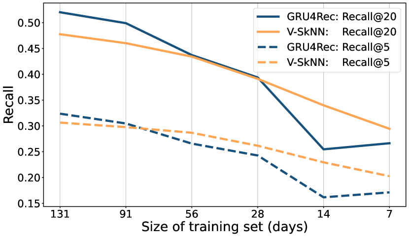
[Accuracy measurements over different training windows]Recall at 5 and 20 values measured for memorization and generalization type algorithms over different training windows.

(a) The effect of using only recent data on the recommendation accuracy of model and neighbor based methods

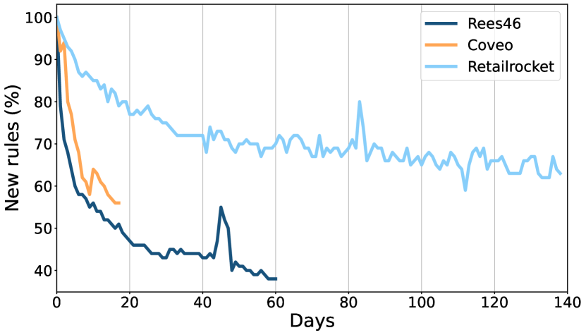
[New rule proportion stops decreasing]After a quick drop, the proportion of new rules stabilizes at a high level.

(b) Proportion of $i\rightarrow j$ item transitions observed first on day $N$ to the number of unique sequences of the same day

Figure 1.

The next step in the design process is the train/test split. Proper evaluation requires eliminating access to any information that would not be available during inference. E.g. training examples must not be used for evaluation. Recommenders should also not have access to future information during evaluation. However, some commonly used splitting strategies (e.g. random split, leave-one-out) inherently enable information leaking through time.

Random splits are appropriate if the preference of users is considered to be long-term and mostly static. This is not the case due to changes in the item catalog, shifting user interest and external factors (e.g. promotions). Figure 1(b) shows the proportion of $i\rightarrow j$ item transitions observed first on day $N$ and the number of unique sequences on the same day. While it declines, it stabilizes on fairly high values, indicating constantly changing user behavior. This concept-drift has been studied by the research community (Gama et al., 2014; Tsymbal, 2004). Overlapping train/test splits lessen the need of modeling the concept drift, and provide an easier, unrealistic problem for which less generalization is needed. Therefore, its effect is not uniform over different types of algorithms.

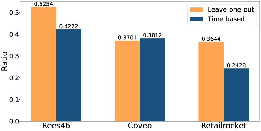
[Bar plot of shared rules]Bar plot of shared rules between training and test sets with leave-one-out having higher overlap

(a) Leave-one-out and time based split

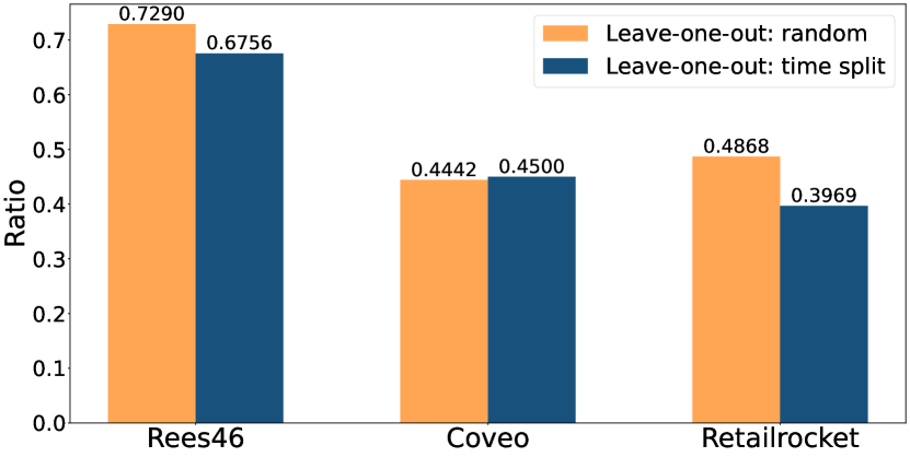
[Bar plot of shared rules]Bar plot of shared rules between training and test sets with random split having higher overlap

(b) Leave-one-out on random vs. most recent sessions

Figure 2. Proportion of the $i\rightarrow j$ test item transitions that are shared with the training set

Leave-one-out splitting is often used in the evaluation of sequential recommenders (Kang and McAuley, 2018; Sun et al., 2019; Huang et al., 2018; Zhou et al., 2020; Li et al., 2020). The last event of the training sequences are moved from the train set to the test set. Sequences end at different times, thus the two sets overlap in time. Figure 2 shows the concept drift between train and test sets as the proportion of the $i\rightarrow j$ test item transitions that are shared with the train set for leave-one-out and time based splits (2(a)); and two variants of the leave-one-out strategy (2(b)) using the most recent and random sequences. Concept drift is significantly smaller for non-overlapping splits of Rees46 and RetailRocket. Coveo has similar proportions for both splits due to consisting of only 18 days of data, which is too short for concept drift to be too prevalent. This clearly indicates that by not requiring strict separation by time, the evaluation setup becomes compromised by information leaking through time, and thus the algorithms are evaluated on a somewhat easier problem than what they would face in a production system.

2.4. Negative sampling during testing

Negative item sampling is a common and severe flaw of the final step, testing. Recently, (Krichene and Rendle, 2020) discussed how sampling introduces bias to measurements and its potential impact on the comparison of algorithms, while (Cañamares and Castells, 2020; Dallmann et al., 2021) demonstrated that it can change the performance based ordering of models. Thus, results achieved with sampling are not reliable. Besides confirming the result of earlier work, we demonstrate how the bias introduced by negative sampling can change the ordering of models, demonstrate its impact, as well as discuss alternatives and whether sampling is needed at all.

This flaw is rooted in the transition from error metrics to IR metrics from a decade ago that brought along a significant increase in the amount of compute needed for evaluation. Opposed to rating prediction that needs only a few score computations per test case, ranking requires scoring all items for every test case, since test items are treated as relevant ones that need to be ranked against other irrelevant items. Different alternatives (Bellogin et al., 2011) were proposed including ranking over all items and ranking the target(s) against a number of sampled negative items. Ranking over all items is how real-life recommenders work, but nevertheless, negative sampling also became a widespread practice, utilized in well cited papers of prestigious conferences (e.g. (Kang and McAuley, 2018; Sun et al., 2019; Huang et al., 2018; Zhou et al., 2020; He et al., 2017; Cai et al., 2022; Rashed et al., 2022)).

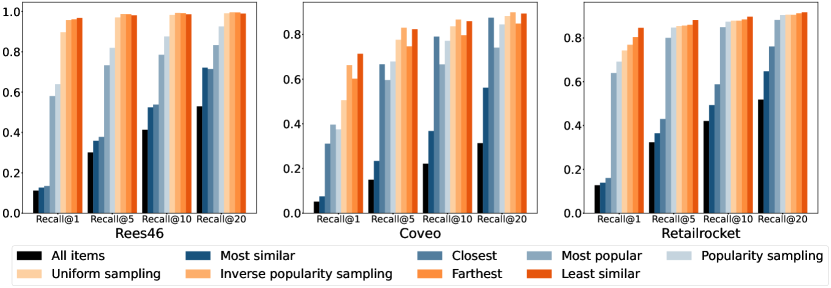
[Bar plot of recall measurements]Bar plot of recall measurements showing that sampling strategies result in overestimating accuracy metrics.

Figure 3. Comparison of the strength of various negative samples of 100 items and no sampling.

Metrics focus on the top few items, thus negative items should be highly ranked for sampled and full ranking results to be similar. Uniform sampling is not able to provide strong samples if the size of the item catalog is significantly larger than the number of samples. The probability of a target item ranked $R$ in the full ranking of $N$ items making it into the recommendation list of $C$ items ($C<R$) when ranked against $S$ negative samples is $\sum_{i=0}^{C-1}{\binom{R-1}{i}\binom{N-R}{S-i}/\binom{N-1}{S}}$. If the target item is ranked $1,490^{\textrm{th}}$ among $10,000$ items or $14,878^{\textrm{th}}$ among $100,000$, it still has more than $90\%$ chance to make it into the top $20$ with $100$ uniform samples. Weak negative samples are easily distinguishable from the target and thus their use results in the severe overestimation of offline accuracy metrics. Using stronger samples provides a more accurate estimation of the accuracy of the non sampled setup. The strength of negative samples – i.e. how hard it is to distinguish them from the target – is depicted on Figure 3 for 8 sampling strategies:

• Sampling strategies: Sampling probability is either uniform or proportional to the items’ support. Popular items are considered to be stronger samples, since recommenders tend to rank them higher.

• Most popular items: The target items are ranked against the $100$ most popular items.

• Similar/close items: Soft upper bound. Requires at least as much compute as full ranking. Items are selected based on the (cosine) similarity or closeness of their embeddings to that of the target item.

• Weak baselines: Soft lower bound. Sampling with probability proportional to reciprocal item support, and items with least similar or farthest embeddings to the target item’s embedding.

Figure 3 indicates that even the computationally expensive most similar and closest approaches can not produce strong item sets consistently. Popularity sampling and most popular items are better than uniform sampling, but these approaches are still not able to estimate the true rank of the target. This can falsify the results, because (1) the difference between the performance of two algorithms can vanish due to the lack of challenging negative items. (2) The relative performance at recommendation list length $M$ shifts to length $N(\ll M)$ because sampling makes it easier to push the target item up on the list. Since the relative performance of two models might depend on the length of the recommendation list, this can also change their ordering for relevant list lengths.

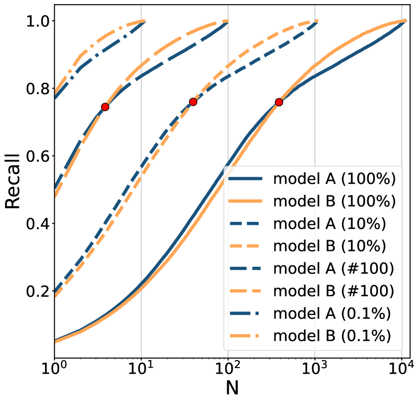
[Recall values at different list length]Recall values at different list length. Algorithm ranking changes at smaller list length as sample size decreases.

(a) Coveo – Recall@N

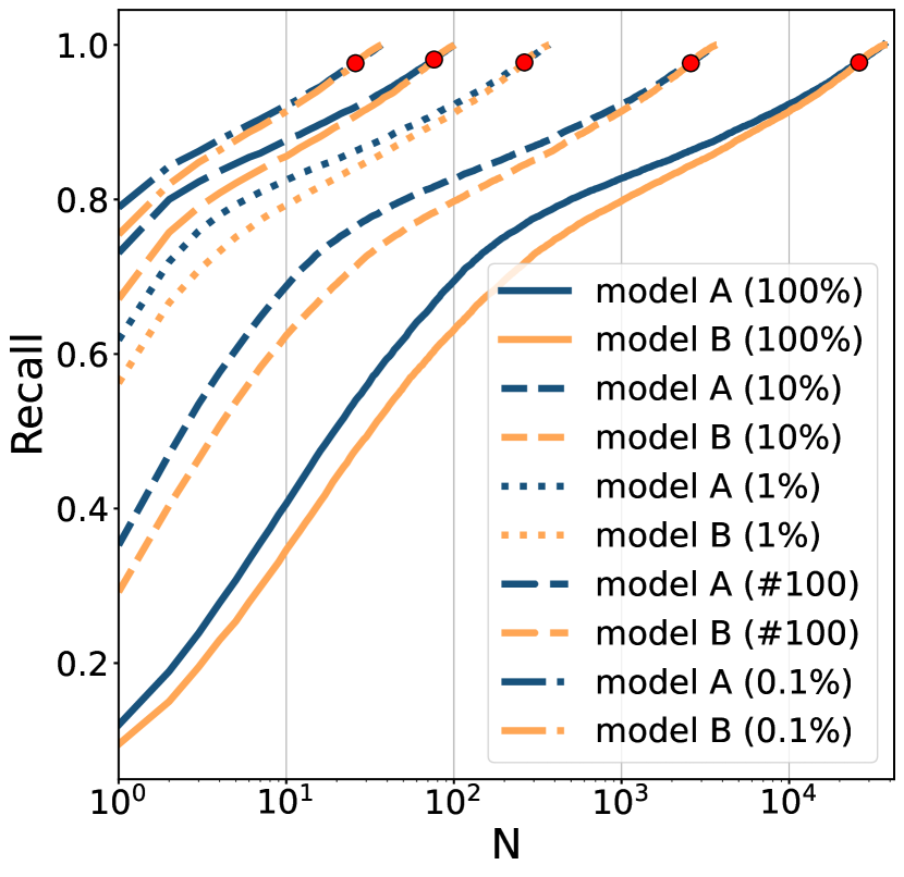
[Recall values at different list length]Recall values at different list length. Algorithm ranking changes at smaller list length as sample size decreases.

(b) Retailrocket – Recall@N

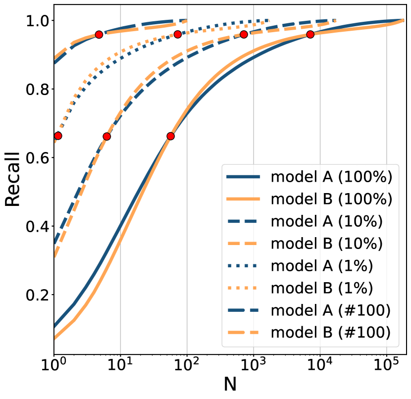
[Recall values at different list length]Recall values at different list length. Algorithm ranking changes at smaller list length as sample size decreases.

(c) Rees46 – Recall@N – AB

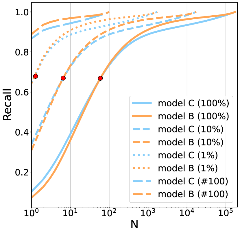
[Recall values at different list length]Recall values at different list length. Algorithm ranking changes at smaller list length as sample size decreases.

(d) Rees46 – Recall@N – BC

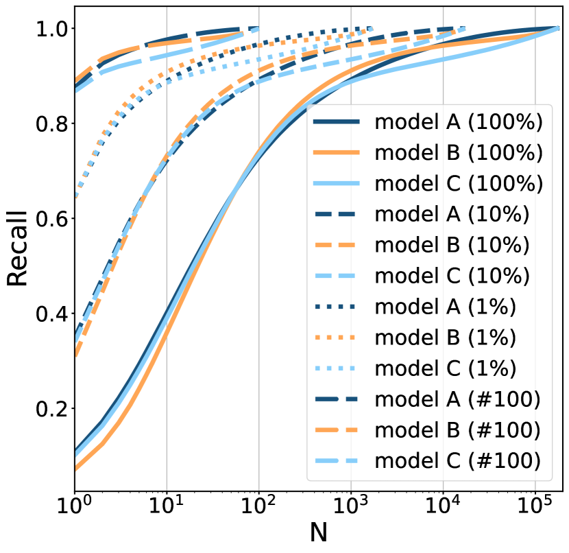
[Recall values at different list length]Recall values at different list length. Algorithm ranking changes at smaller list length as sample size decreases.

(e) Rees46 – Recall@N – ALL

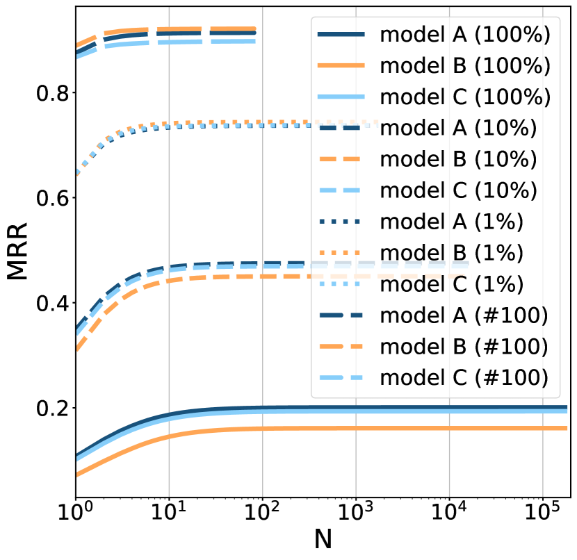
[MRR values at different list length]MRR values at different list length. Algorithm ranking changes as sample size decreases.

(f) Rees46 – MRR@N – ALL

Figure 4. Accuracy as the function of recommendation list length, with and without sampling

Figure 4 demonstrates this point by showing recall@N as the function of $N$ for pairs of models for full ranking ($100\%$), and for randomly sampling $10\%$, $1\%$, $0.1\%$ of the item catalog or $100$ items. The ordering of models is not static over $N$, and it might change multiple times (marked by red dots). Decreasing sample size moves these intersections to the left, pushing the change in model ordering to lower $N$ values. Changes to the relative performance are drastic: model A on Coveo (4(a)) outperforms model B by $8.1\%$ in recall@20, but A underperforms B by $4.7\%$ when $100$ negative samples are used. While the ordering of model A and B does not change for Retailrocket (4(b)), $14.3\%$ uplift in recall@20 vanishes and drops to $1.5\%$. The biggest change can be observed between model A and B on Rees46 (4(c)) where the uplift in recall@1 (and MRR@1) drops from $49.5\%$ to $-1.6\%$. Since MRR is even more sensitive to the top of the list, this affects relative MRR based performance for any $N$: the true order of models A, B and C on Rees46 (4(f)) is $A>C\gg B$, but with $100$ samples it reads as $B>A\gg C$.

Computational complexity of evaluation via full ranking depends on the number of test recommendations and the size of the item catalog. Most public dataset are quite small, and even the bigger ones have item catalogs of easily manageable sizes. One test on Rees46 requires $887,369$ recommendation lists over $172,756$ items each that is executed in only $205.1$ seconds on an A30 GPU. Even before GPUs, evaluation on public datasets of the time could be executed in a few minutes using optimized code. If a dataset is really too large for quick experimentation, the sampling of test recommendations (e.g. users) gives more representative results. Certain scoring models are not designed for full ranking. If one such model must be evaluated on ranking, generating candidate sets via another algorithm can solve the problem. However, this limits the generality of claims about its performance, because currently there are no universally accepted candidate set generators.

3. Related work

Offline evaluation of top-N recommenders has been discussed since top-N recommendation became dominant. Early works mainly focused on metrics (Hurley and Zhang, 2011; Vargas and Castells, 2011) and finding connections between offline and online results (Rossetti et al., 2016). The pace of the work has increased in recent years (Zangerle et al., 2022), simultaneously with the sharp increase of papers lacking satisfactory evaluation.

Evaluation has many aspects from metrics (Hurley and Zhang, 2011; Vargas and Castells, 2011) to hyperparameter optimization (Rendle et al., 2022). (Ferrari Dacrema et al., 2019, 2020) suggests that one of the reasons behind the low reproducibility rate of recent papers is that evaluation setups are lifted from earlier work without their validity being checked.

Our work focuses on this problem, i.e. the design of evaluation setups and the flaws within. Of the four flaws discussed in this paper, only negative item sampling has been scrutinized, aside from (Tang and Wang, 2018) briefly mentioning that the Amazon dataset has weak sequential signals. (Krichene and Rendle, 2020) discussed the background of how sampling introduces bias to measurements, and (Cañamares and Castells, 2020; Dallmann et al., 2021) demonstrated that the relative performance of models can change when sampling is applied. Our experiments confirm their results and give additional explanation on why this change happens.

4. Discussion & Conclusion

Offline evaluation is fundamentally imperfect, but it will likely remain the main approach for assessing performance in recommendation systems research. Online A/B tests are not just expensive and slow, but inherently not reproducible; and simulators are still in their early stages. Unfortunately, flaws are quite widespread in offline evaluation setups. In this paper, we went through the main steps of designing evaluation setups and pointed out four widespread flaws and demonstrated their effect through the example of sequential recommendations. We chose sequential recommendation for the demonstration, because it is one of the areas severely plagued by low quality evaluation. Evaluation flaws of some of the earlier sequential recommender papers – e.g. (Kang and McAuley, 2018) has all four we discussed – were missed by both the authors and reviewers. Later works copied the setups – with their flaws included – without questioning whether they are correct. There is not a single best way for offline evaluation, but by pointing out these four flaws, we hope to see the quality of experimentation sections of research papers improving in the future.

- (1)
- Bellogin et al. (2011) Alejandro Bellogin, Pablo Castells, and Ivan Cantador. 2011. Precision-oriented evaluation of recommender systems: an algorithmic comparison. In Proceedings of the fifth ACM conference on Recommender systems. 333–336.
- Cai et al. (2022) Wei Cai, Weike Pan, Jingwen Mao, Zhechao Yu, and Congfu Xu. 2022. Aspect Re-distribution for Learning Better Item Embeddings in Sequential Recommendation. In Proceedings of the 16th ACM Conference on Recommender Systems. 49–58.
- Cañamares and Castells (2020) Rocío Cañamares and Pablo Castells. 2020. On target item sampling in offline recommender system evaluation. In Proceedings of the 14th ACM Conference on Recommender Systems. 259–268.
- Chen et al. (2021) Minmin Chen, Yuyan Wang, Can Xu, Ya Le, Mohit Sharma, Lee Richardson, Su-Lin Wu, and Ed Chi. 2021. Values of User Exploration in Recommender Systems. In Proceedings of the 15th ACM Conference on Recommender Systems (Amsterdam, Netherlands) (RecSys ’21). Association for Computing Machinery, New York, NY, USA, 85–95. https://doi.org/10.1145/3460231.3474236
- Dallmann et al. (2021) Alexander Dallmann, Daniel Zoller, and Andreas Hotho. 2021. A case study on sampling strategies for evaluating neural sequential item recommendation models. In Proceedings of the 15th ACM Conference on Recommender Systems. 505–514.
- Ferrari Dacrema et al. (2019) Maurizio Ferrari Dacrema, Paolo Cremonesi, and Dietmar Jannach. 2019. Are we really making much progress? A worrying analysis of recent neural recommendation approaches. In Proceedings of the 13th ACM conference on recommender systems. 101–109.
- Ferrari Dacrema et al. (2020) Maurizio Ferrari Dacrema, Paolo Cremonesi, Dietmar Jannach, et al. 2020. Methodological issues in recommender systems research. In IJCAI, Vol. 2021. International Joint Conferences on Artificial Intelligence, 4706–4710.
- Gama et al. (2014) João Gama, Indrė Žliobaitė, Albert Bifet, Mykola Pechenizkiy, and Abdelhamid Bouchachia. 2014. A survey on concept drift adaptation. ACM computing surveys (CSUR) 46, 4 (2014), 1–37.
- Guo et al. (2017) Huifeng Guo, Ruiming Tang, Yunming Ye, Zhenguo Li, and Xiuqiang He. 2017. DeepFM: a factorization-machine based neural network for CTR prediction. arXiv preprint arXiv:1703.04247 (2017).
- He et al. (2017) Xiangnan He, Lizi Liao, Hanwang Zhang, Liqiang Nie, Xia Hu, and Tat-Seng Chua. 2017. Neural collaborative filtering. In Proceedings of the 26th international conference on world wide web. 173–182.
- He et al. (2016) Xiangnan He, Hanwang Zhang, Min-Yen Kan, and Tat-Seng Chua. 2016. Fast matrix factorization for online recommendation with implicit feedback. In Proceedings of the 39th International ACM SIGIR conference on Research and Development in Information Retrieval. 549–558.
- Hidasi and Karatzoglou (2018) Balázs Hidasi and Alexandros Karatzoglou. 2018. Recurrent neural networks with top-k gains for session-based recommendations. In Proceedings of the 27th ACM international conference on information and knowledge management. 843–852.
- Hidasi et al. (2015) Balázs Hidasi, Alexandros Karatzoglou, Linas Baltrunas, and Domonkos Tikk. 2015. Session-based recommendations with recurrent neural networks. arXiv preprint arXiv:1511.06939 (2015).
- Hidasi and Tikk (2012) Balázs Hidasi and Domonkos Tikk. 2012. Fast ALS-based tensor factorization for context-aware recommendation from implicit feedback. In Machine Learning and Knowledge Discovery in Databases: European Conference, ECML PKDD 2012, Bristol, UK, September 24-28, 2012. Proceedings, Part II 23. Springer, 67–82.
- Hu et al. (2008) Yifan Hu, Yehuda Koren, and Chris Volinsky. 2008. Collaborative filtering for implicit feedback datasets. In 2008 Eighth IEEE international conference on data mining. Ieee, 263–272.
- Huang et al. (2018) Jin Huang, Wayne Xin Zhao, Hongjian Dou, Ji-Rong Wen, and Edward Y Chang. 2018. Improving sequential recommendation with knowledge-enhanced memory networks. In The 41st international ACM SIGIR conference on research & development in information retrieval. 505–514.
- Hurley and Zhang (2011) Neil Hurley and Mi Zhang. 2011. Novelty and diversity in top-n recommendation–analysis and evaluation. ACM Transactions on Internet Technology (TOIT) 10, 4 (2011), 1–30.
- Jeunen (2023) Olivier Jeunen. 2023. A Common Misassumption in Online Experiments with Machine Learning Models. arXiv preprint arXiv:2304.10900 (2023).
- Kang and McAuley (2018) Wang-Cheng Kang and Julian McAuley. 2018. Self-attentive sequential recommendation. In 2018 IEEE international conference on data mining (ICDM). IEEE, 197–206.
- Krichene and Rendle (2020) Walid Krichene and Steffen Rendle. 2020. On sampled metrics for item recommendation. In Proceedings of the 26th ACM SIGKDD international conference on knowledge discovery & data mining. 1748–1757.
- Li et al. (2020) Jiacheng Li, Yujie Wang, and Julian McAuley. 2020. Time interval aware self-attention for sequential recommendation. In Proceedings of the 13th international conference on web search and data mining. 322–330.
- Ludewig and Jannach (2018) Malte Ludewig and Dietmar Jannach. 2018. Evaluation of session-based recommendation algorithms. User Modeling and User-Adapted Interaction 28 (2018), 331–390.
- McInerney et al. (2021) James McInerney, Ehtsham Elahi, Justin Basilico, Yves Raimond, and Tony Jebara. 2021. Accordion: a trainable simulator for long-term interactive systems. In Proceedings of the 15th ACM Conference on Recommender Systems. 102–113.
- Petrov and Macdonald (2022) Aleksandr Petrov and Craig Macdonald. 2022. A Systematic Review and Replicability Study of BERT4Rec for Sequential Recommendation. In Proceedings of the 16th ACM Conference on Recommender Systems. 436–447.
- Pilászy et al. (2010) István Pilászy, Dávid Zibriczky, and Domonkos Tikk. 2010. Fast als-based matrix factorization for explicit and implicit feedback datasets. In Proceedings of the fourth ACM conference on Recommender systems. 71–78.
- Rashed et al. (2022) Ahmed Rashed, Shereen Elsayed, and Lars Schmidt-Thieme. 2022. Context and Attribute-Aware Sequential Recommendation via Cross-Attention. In Proceedings of the 16th ACM Conference on Recommender Systems. 71–80.
- Rendle et al. (2022) Steffen Rendle, Walid Krichene, Li Zhang, and Yehuda Koren. 2022. Revisiting the performance of ials on item recommendation benchmarks. In Proceedings of the 16th ACM Conference on Recommender Systems. 427–435.
- Requena et al. (2020) Borja Requena, Giovanni Cassani, Jacopo Tagliabue, Ciro Greco, and Lucas Lacasa. 2020. Shopper intent prediction from clickstream e-commerce data with minimal browsing information. Scientific reports 10, 1 (2020), 1–23.
- Rossetti et al. (2016) Marco Rossetti, Fabio Stella, and Markus Zanker. 2016. Contrasting Offline and Online Results When Evaluating Recommendation Algorithms. In Proceedings of the 10th ACM Conference on Recommender Systems (Boston, Massachusetts, USA) (RecSys ’16). Association for Computing Machinery, New York, NY, USA, 31–34. https://doi.org/10.1145/2959100.2959176
- Saito and Joachims (2021) Yuta Saito and Thorsten Joachims. 2021. Counterfactual learning and evaluation for recommender systems: Foundations, implementations, and recent advances. In Proceedings of the 15th ACM Conference on Recommender Systems. 828–830.
- Sun et al. (2019) Fei Sun, Jun Liu, Jian Wu, Changhua Pei, Xiao Lin, Wenwu Ou, and Peng Jiang. 2019. BERT4Rec: Sequential recommendation with bidirectional encoder representations from transformer. In Proceedings of the 28th ACM international conference on information and knowledge management. 1441–1450.
- Tan et al. (2016) Yong Kiam Tan, Xinxing Xu, and Yong Liu. 2016. Improved recurrent neural networks for session-based recommendations. In Proceedings of the 1st workshop on deep learning for recommender systems. 17–22.
- Tang and Wang (2018) Jiaxi Tang and Ke Wang. 2018. Personalized top-n sequential recommendation via convolutional sequence embedding. In Proceedings of the eleventh ACM international conference on web search and data mining. 565–573.
- Tsymbal (2004) Alexey Tsymbal. 2004. The problem of concept drift: definitions and related work. Computer Science Department, Trinity College Dublin 106, 2 (2004), 58.
- Vargas and Castells (2011) Saúl Vargas and Pablo Castells. 2011. Rank and relevance in novelty and diversity metrics for recommender systems. In Proceedings of the fifth ACM conference on Recommender systems. 109–116.
- Wan and McAuley (2018) Mengting Wan and Julian McAuley. 2018. Item recommendation on monotonic behavior chains. In Proceedings of the 12th ACM conference on recommender systems. 86–94.
- Wang et al. (2019) Xiang Wang, Xiangnan He, Meng Wang, Fuli Feng, and Tat-Seng Chua. 2019. Neural graph collaborative filtering. In Proceedings of the 42nd international ACM SIGIR conference on Research and development in Information Retrieval. 165–174.
- Zangerle et al. (2022) Eva Zangerle, Christine Bauer, and Alan Said. 2022. Second Workshop: Perspectives on the Evaluation of Recommender Systems (PERSPECTIVES 2022). In Proceedings of the 16th ACM Conference on Recommender Systems (Seattle, WA, USA) (RecSys ’22). Association for Computing Machinery, New York, NY, USA, 652–653. https://doi.org/10.1145/3523227.3547408
- Zhou et al. (2020) Kun Zhou, Hui Wang, Wayne Xin Zhao, Yutao Zhu, Sirui Wang, Fuzheng Zhang, Zhongyuan Wang, and Ji-Rong Wen. 2020. S3-rec: Self-supervised learning for sequential recommendation with mutual information maximization. In Proceedings of the 29th ACM international conference on information & knowledge management. 1893–1902.