Study of the nonleptonic decay $\Xi^{0}_{c}\to\Lambda^{+}_{c}\pi^{-}$ in the covariant confined quark model

Abstract

The nonleptonic decay $\Xi^{0}_{c}\to\Lambda^{+}_{c}\pi^{-}$ with $\Delta C=0$ is systematically studied in the framework of the covariant confined quark model accounting for both short and long distance effects. The short distance effects are induced by four topologies of external and internal weak $W^{\pm}$ exchange, while long distance effects are saturated by an inclusion of the so-called pole diagrams with an intermediate $\frac{1}{2}^{+}$ and $\frac{1}{2}^{-}$ baryon resonances. The contributions from $\frac{1}{2}^{+}$ resonances are calculated straightforwardly by accounting for single charmed $\Sigma^{0}_{c}$ and $\Xi^{{}^{\prime}\,+}_{c}$ baryons whereas the contributions from $\frac{1}{2}^{-}$ resonances are calculated by using the well-known soft-pion theorem in the current-algebra approach. It allows to express the parity-violating S-wave amplitude in terms of parity-conserving matrix elements. It is found that the contribution of external and internal $W$-exchange diagrams is significantly suppressed by more than one order of magnitude in comparison with data. The pole diagrams play the major role to get consistency with experiment.

I   Introduction

The study of the heavy-flavor-conserving nonleptonic weak decays of heavy baryons has received a lot of attention due to their observation and measurement of branching fractions by the LHCb and Belle collaborations. The decay $\Xi^{0}_{c}\to\Lambda^{+}_{c}+\pi^{-}$ was first observed at LHCb experiment and the branching fraction was measured to be ${\mathcal{B}}=(0.55\pm 0.02\pm 0.18)\%$ LHCb:2020gge . Recent experimental data obtained by the Belle collaboration gave the value of ${\mathcal{B}}(\Xi^{0}_{c}\to\Lambda^{+}_{c}+\pi^{-})=(0.54\pm 0.05\pm 0.12)\%$ Belle:2022kqi which is in perfect agreement with the LHCb result.

The recent theoretical review of nonleptonic two-body decays of single and doubly charm baryons was given in Ref. Groote:2021pxt . The review was aiming to shed new light on the standard current algebra approach to such processes.

The heavy-flavor-conserving nonleptonic weak decays of heavy baryons were studied in Cheng:1992ff in the formalism which incorporates both the heavy quark symmetry and the chiral symmetry. The branching fractions of specific nonleptonic decays such as $\Xi_{c}\to\Lambda^{+}_{c}\pi$ are found to be of the order of $10^{-4}$.

The weak decays $\Xi_{b}\to\Lambda_{b}\pi$ and $\Xi_{c}\to\Lambda^{+}_{c}\pi$, in which the heavy quark is not destroyed, have been discussed in Ref. Voloshin:2000et . It was shown that these should go at the rate of order $\approx 0.01\,\text{ps}^{-1}$. In the updated research Voloshin:2019ngb of the Voloshin’s approach, the new measurements by LHCb LHCb:2019ldj of the lifetimes of the $\Lambda_{c}^{+}$, $\Xi_{c}^{+}$ and $\Xi_{c}^{0}$ charm baryons have been used to predict a lower bound on the rate of the decays $\Xi^{0}_{c}\to\Lambda^{+}_{c}\pi$. It was found that ${\mathcal{B}}(\Xi^{0}_{c}\to\Lambda^{+}_{c}+\pi^{-})>{\mathcal{B}}_{\rm min}=(0.25\pm 0.15)\times 10^{-3}$.

The heavy flavor conserving decays of strange charmed baryons proceed via two subprocesses, first, via decay $s\to u(\bar{u}d)$ (or equivalently, via the transition $us\to ud$), and, second, via the transition $cs\to cd$. In Ref. Gronau:2016xiq it was shown that a second term is approximately equal to the first term. But it was unclear whether they interfere destructively or constructively. For constructive interference it was found that ${\mathcal{B}}(\Xi^{0}_{c}\to\Lambda^{+}_{c}+\pi^{-})=(1.94\pm 0.70)\times 10^{-3}$. For destructive interference, the value of branching fraction is expected to be less than about $10^{-4}$.

In Ref. Faller:2015oma the upper bound for the decay width $\Gamma(\Xi^{0}_{c}\to\Lambda^{+}_{c}+\pi^{-})<1.7\times 10^{-14}$ GeV was obtained by using the Voloshin’s approach. In work Cheng:2015ckx the four-quark matrix element of heavy-flavor-conserving hadronic weak decays was evaluated in using two different models: the MIT bag model and the diquark model. All calculations included only S-wave amplitudes and obtained $\mathcal{B}(\Xi^{0}_{c}\to\Lambda^{+}_{c}+\pi^{-})=1.7\times 10^{-7}$ for MIT bag model and $\mathcal{B}(\Xi^{0}_{c}\to\Lambda^{+}_{c}+\pi^{-})=0.87\times 10^{-4}$ for diquark model. In updated work Cheng:2022kea it was confirmed that $\Xi_{c}\to\Lambda^{+}_{c}\pi$ decays are indeed dominated by the parity-conserving transition induced from nonspectator $W$-exchange and that they receive largest contributions from the intermediate $\Sigma^{0}_{c}$ pole terms. Also they obtained that the asymmetry parameter $\alpha$ is positive, of order $0.70^{+0.13}_{-0.17}$ and $\mathcal{B}(\Xi^{0}_{c}\to\Lambda^{+}_{c}+\pi^{-})=1.76^{+0.18}_{-0.12}\times 10^{-3}$. In Cheng:2022jbr the wave functions from the homogeneous bag model are adopted in order to remove the center-of-mass motion of the static bag. The calculations have been carried out under the same framework, and it has been shown that the matrix elements of four-quark operators are enhanced about twice and for $\mathcal{B}(\Xi^{0}_{c}\to\Lambda^{+}_{c}+\pi^{-})=(7.2\pm 0.7)\times 10^{-3}$.

It was investigated pion emission and pole terms in the heavy quark conserving weak decay of $\Xi^{0}_{c}$ in the framework of non-relativistic constituent quark model Niu:2021qcc . The parity-conserving pole terms are found dominant and the direct pion emission contributions are rather small and $\mathcal{B}(\Xi^{0}_{c}\to\Lambda^{+}_{c}+\pi^{-})=(0.58\pm 0.21)\%$ with uncertainties caused by the quark model parameters with 20% errors.

This work is aiming to study the decay $\Xi^{0}_{c}\to\Lambda^{+}_{c}+\pi^{-}$ in the framework of the covariant confined quark model (CCQM) previously developed by us, see Ref. Branz:2009cd . This approach found many applications, particularly, in physics of heavy baryons, see Refs. Gutsche:2018msz ; Ivanov:2021huf ; Gutsche:2015mxa ; Ivanov:2020xmw ; Ivanov:2020iaq ; Gutsche:2019iac ; Gutsche:2019wgu ; Gutsche:2018utw ; Ivanov:2017axg ; Gutsche:2017hux ; Gutsche:2017wag ; Gutsche:2015rrt ; Gutsche:2015lea ; Habyl:2015xka ; Gutsche:2014zna ; Gutsche:2013oea ; Gutsche:2013pp ; Gutsche:2012ze . One of the important step in development of the CCQM was done in Ref. Gutsche:2018msz where ab initio three-loop quark model calculation of the $W$-exchange contribution to the nonleptonic two-body decays of the doubly charmed baryons $\Xi_{cc}^{++}$ and $\Omega_{cc}^{+}$ have been made. The $W$-exchange contributions appear in addition to the factorizable contributions and, generally, are not suppressed. In Ivanov:2021huf such an approach was extended to study two-body nonleptonic decays of light lambda hyperon $\Lambda\to p\pi^{-}(n\pi^{0})$ with account for both short and long distance effects. It was shown that the contribution from the $W$-exchange diagrams is sizably suppressed and basically the pole diagrams allow to describe the experimental data for the branching fractions.

The paper is organized as follows. In Sec. II we briefly discuss the classification and spectroscopy of singly charmed $1/2^{+}$ baryons. Then we give the basic ingredients and milestones that are needed for calculation of two-body nonleptonic decays including both the $W$-exchange quark and pole diagrams. Sec. III is devoted to calculation of the matrix elements and branching fraction of the decay $\Xi^{0}_{c}\to\Lambda^{+}_{c}+\pi^{-}$. We discuss in details the classification of the diagrams appearing in these decays and give the analytical expressions for matrix elements. In Sec. IV we present numerical results for the amplitudes and branching fractions. We compare them with those available in the literature. Finally, in Sec. V we make conclusions and summarize the main results obtained in this paper.

II   The singly charmed baryons

The masses of singly charmed baryons have been predicted in one gluon exchange model developed in Ref. DeRujula:1975qlm . The comprehensive review on heavy baryons, their spectroscopy, semileptonic and nonleptonic decays may be found in Ref. Korner:1994nh . In Tables 1 we display the names, quark contents and interpolating currents of the low-lying multiplets of singly charmed baryons with spin 1/2. For singly charmed baryons the flavor decomposition of the diquark, made of $(u,d,s)$-quarks is $3\otimes 3=\bar{3}_{A}+6_{S}$ (A=antisymmetric, S=symmetric). The values of masses with errors are taken from particle data group (PDG) ParticleDataGroup:2022pth .

Table 1: Singly charmed $1/2^{+}$ baryon states. Notation $[a,b]$ and $\{a,b\}$ for antisymmetric and symmetric flavor index combinations.

Title	Content	$SU(3)$	$(I,I_{3})$	Current	Mass (MeV)
$\Lambda^{+}_{c}$	$c[ud]$	$\bar{3}$	(0,0)	$\epsilon^{abc}c^{a}(u^{b}C\gamma_{5}d^{c})$	2286.46 $\pm$ 0.14
$\Xi_{c}^{+}$	$c[us]$	$\bar{3}$	(1/2,1/2)	$\epsilon^{abc}c^{a}(u^{b}C\gamma_{5}s^{c}$)	2467.71 $\pm$ 0.23
$\Xi_{c}^{0}$	$c[ds]$	$\bar{3}$	(1/2,–1/2)	$\epsilon^{abc}c^{a}(d^{b}C\gamma_{5}s^{c}$)	2470.44 $\pm$ 0.28
$\Sigma_{c}^{++}$	$cuu$	6	(1,1)	$\epsilon^{abc}\gamma_{\mu}\gamma_{5}c^{a}(u^{b}C\gamma^{\mu}u^{c})$	2453.97 $\pm$ 0.14
$\Sigma_{c}^{+}$	$c\{ud\}$	6	(1,0)	$\epsilon^{abc}\gamma_{\mu}\gamma_{5}c^{a}(u^{b}C\gamma^{\mu}d^{c})$	2452.65 $\pm$ 0.22
$\Sigma_{c}^{0}$	$cdd$	6	(1,–1)	$\epsilon^{abc}\gamma_{\mu}\gamma_{5}c^{a}(d^{b}C\gamma^{\mu}d^{c})$	2453.75 $\pm$ 0.14
$\Xi_{c}^{\prime\,+}$	$c\{us\}$	6	(1/2,1/2)	$\epsilon^{abc}\gamma_{\mu}\gamma_{5}c^{a}(u^{b}C\gamma^{\mu}s^{c})$	2578.2 $\pm$ 0.5
$\Xi_{c}^{\prime\,0}$	$c\{ds\}$	6	(1/2,–1/2)	$\epsilon^{abc}\gamma_{\mu}\gamma_{5}c^{a}(d^{b}C\gamma^{\mu}s^{c})$	2578.7 $\pm$ 0.5
$\Omega_{c}^{0}$	$css$	6	(0,0)	$\epsilon^{abc}\gamma_{\mu}\gamma_{5}c^{a}(s^{b}C\gamma^{\mu}s^{c})$	2695.2 $\pm$ 1.7

We are aiming to study the two-body nonleptonic decay $\Xi^{0}_{c}\to\Lambda^{+}_{c}\pi^{-}$ which branching fraction was measured for the first time by LHCb collaboration LHCb:2020gge . The effective Hamiltonian relevant for this purpose is written as

$$\mathcal{H}^{\Delta\rm S=1}_{\rm eff} = \frac{G_{F}}{\sqrt{2}}\left[\,\,V^{\ast}_{us}V_{ud}\left(C^{(u)}_{1}(\mu_{u})Q^{(u)}_{1}+C^{(u)}_{2}(\mu_{u})Q^{(u)}_{2}\right)\right.$$ (1)

$$\left.\phantom{\frac{G_{F}}{\sqrt{2}}}+V^{\ast}_{cs}V_{cd}\left(C^{(c)}_{1}(\mu_{c})Q^{(c)}_{1}+C^{(c)}_{2}(\mu_{c})Q^{(c)}_{2}\right)+{\rm H.c.}\right]$$

where $Q_{1}$ and $Q_{2}$ is the set of flavor-changing effective four-quark operators given by

$$Q^{(u)}_{1} = (\bar{s}_{a}O_{L}^{\mu}u_{b})(\bar{u}_{b}O_{\mu L}d_{a}),\qquad Q^{(u)}_{2}=(\bar{s}_{a}O_{L}^{\mu}u_{a})(\bar{u}_{b}O_{\mu L}d_{b}),$$

$$Q^{(c)}_{1} = (\bar{s}_{a}O_{L}^{\mu}c_{b})(\bar{c}_{b}O_{\mu L}d_{a}),\qquad Q^{(c)}_{2}=(\bar{s}_{a}O_{L}^{\mu}c_{a})(\bar{c}_{b}O_{\mu L}d_{b}).$$ (2)

Here $O_{L}^{\mu}=\gamma^{\mu}(1-\gamma_{5})$ is the left-handed chiral weak matrix. One has to note that we adopt the numeration of the operators from Ref. Buchalla:1995vs where the $C_{2}Q_{2}$ means the leading order whereas the $C_{1}Q_{1}$ is for subleading order. The numerical values of the Wilson coefficients $C_{1}$ and $C_{2}$ from Ref. Buchalla:1995vs are being equal to

$$C^{(u)}_{1}(\mu_{u}) = -0.625,\qquad C^{(u)}_{2}(\mu_{u})=1.361,\quad(\mu_{u}=O(1\,\text{GeV})),$$

$$C^{(c)}_{1}(\mu_{c}) = -0.621,\qquad C^{(c)}_{2}(\mu_{c})=1.336,\quad(\mu_{c}=O(m_{c})).$$ (3)

We do not include penguin operators because their Wilson coefficients are small compare with those from current-current operators.

In the standard model (SM) the relation $V_{cs}^{\ast}V_{cd}=-V_{us}^{\ast}V_{ud}$ holds to an excellent approximation. For instance, in the Wolfenstein parametrization of the Cabibbo-Kobayashi-Maskawa (CKM) matrix, one has $V_{us}^{\ast}V_{ud}=+\lambda(1-\lambda^{2})+O(\lambda^{4})$ whereas $V_{cs}^{\ast}V_{cd}=-\lambda(1-\lambda^{2})+O(\lambda^{4}).$ The global fit in the SM for the Wolfenstein parameter gives $\lambda=0.22500\pm 0.00067$. In what follows, we introduce the short notations

$$V_{\rm CKM}^{(u)}=|V_{us}^{\ast}V_{ud}|,\quad\text{and}\quad V_{\rm CKM}^{(c)}=-|V_{cs}^{\ast}V_{cd}|.$$ (4)

The numerical values of the CKM matrix elements needed in our calculations are taken from PDG ParticleDataGroup:2022pth :

$$|V_{ud}| =0.97373\pm 0.00031, |V_{us}| =0.2243\pm 0.0008,$$

$$|V_{cd}| =0.221\pm 0.004, |V_{cs}| =0.975\pm 0.006,$$ (5)

that approximately give $V_{\rm CKM}^{(u)}\approx 0.218$ and $V_{\rm CKM}^{(c)}\approx-0.215$.

The quark diagrams that contribute to the Cabibbo-favored decay are shown in Fig. 1. After hadronizarion, the diagram Ia factorizes out into two parts: the weak transition $\Xi_{c}^{0}\to\Lambda_{c}^{+}$ via the $W$-emission and the matrix element describing the pion leptonic decay. The $W$-exchange diagrams IIa, IIb and III contribute into both the pure quark diagrams called the short distance (SD) contributions and effectively into the pole diagrams shown in Fig. 2. They describe the so-called long distance (LD) contributions. For instance, the diagrams IIa and III effectively generate the $\Sigma^{0}_{c}$-resonance diagram, whereas the diagram IIb effectively generates the $\Xi_{c}^{+}$ and $\Xi_{c}^{\prime\,+}$-resonance diagrams.

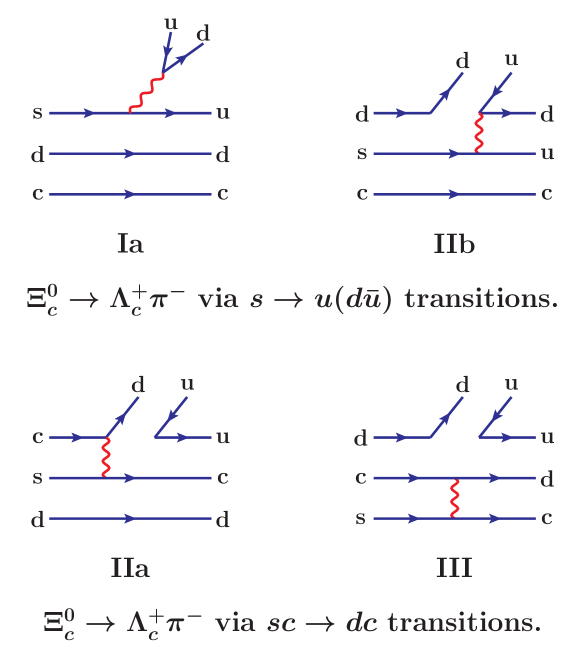
Figure 1: Flavor-color topologies for $\Xi^{0}_{c}\to\Lambda_{c}^{+}\pi^{-}$ decay: Ia is the tree level diagram, IIa, IIb and III are the $W$-exchange diagrams.

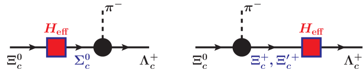
Figure 2: The pole diagrams which effectively account for the long-distance contributions.

III   Matrix elements and decay widths

We are going to calculate the matrix elements of nonleptonic decays of $\Xi^{0}_{c}$-baryon in the framework of the CCQM developed in our previous papers. The starting point is the Lagrangian describing couplings of the baryon field with its interpolating quark current.

$${\cal L}(x)=g_{B}\bar{B}(x)\,J(x)+{\rm H.c.}\,,$$ (6)

where the coupling constant $g_{B}$ is determined from the so-called compositeness condition, which was proposed by Salam and Weinberg Salam:1962ap ; Weinberg:1962hj and extensively used in the literature (see, e.g., Refs. Hayashi:1967hk ; Efimov:1993ei ).

The nonlocal extension of the interpolating currents shown in Table 1 reads

$$J_{B}(x) = \int\!\!dx_{1}\!\!\int\!\!dx_{2}\!\!\int\!\!dx_{3}\,F_{B}(x;x_{1},x_{2},x_{3})\,\varepsilon_{abc}\,\Gamma_{1}q_{1}^{a}(x_{1})\,\left(q_{2}^{b}(x_{2})\,C\Gamma_{2}\,q_{3}^{c}(x_{3})\right)\,,$$

$$F_{B}(x;x_{1},x_{2},x_{3}) = \delta^{(4)}\Big{(}x-\sum\limits_{i=1}^{3}w_{i}x_{i}\Big{)}\Phi_{B}\Big{(}\sum\limits_{i<j}(x_{i}-x_{j})^{2}\Big{)}\,,$$ (7)

where $w_{i}=m_{i}/(\sum_{j=1}^{3}m_{j})$ and $m_{i}$ is the mass of the quark at the space-time point $x_{i}$. The matrices $\Gamma_{1},\Gamma_{2}$ are the Dirac strings of the initial and final baryon states as specified in Table 1. The vertex function $\Phi_{B}$ is written as

$$\Phi_{B}\Big{(}\sum\limits_{i<j}(x_{i}-x_{j})^{2}\Big{)}=\int\!\frac{dq_{1}}{(2\pi)^{4}}\int\!\frac{dq_{2}}{(2\pi)^{4}}e^{-iq_{1}(x_{1}-x_{3})-iq_{2}(x_{2}-x_{3})}\widetilde{\Phi}_{B}\Big{(}-\vec{\Omega}_{q}^{2}\Big{)}\,,$$

$$\widetilde{\Phi}_{B}\Big{(}-\vec{\Omega}_{q}^{2}\Big{)}=\exp\left(\vec{\Omega}_{q}^{2}/\Lambda_{B}^{2}\right),\qquad\vec{\Omega}_{q}^{2}=\tfrac{1}{2}(q_{1}+q_{2})^{2}+\tfrac{1}{6}(q_{1}-q_{2})^{2}=\frac{2}{3}\sum\limits_{i\leq j}q_{i}q_{j}\,.$$ (8)

For simplicity and calculational advantages we mostly adopted a Gaussian form for the functions $\widetilde{\Phi}_{B}$. Here $\Lambda_{B}$ is the size parameter for a given baryon. The size parameter phenomenologically describes the distribution of the constituent quarks in the given baryon.

In our approach the matrix elements contributing to the baryon transitions $\Xi^{0}_{c}\to\Lambda_{c}^{+}\pi^{-}$ are represented by a set of the quark diagrams shown in Fig. 3. They describe the so-called short distance contributions.

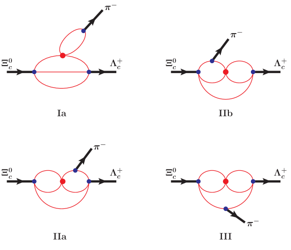
Figure 3: Quark diagrams describing the SD-contributions

The diagrams describing the building blocks of the LD-contributions are shown in Fig. 4.

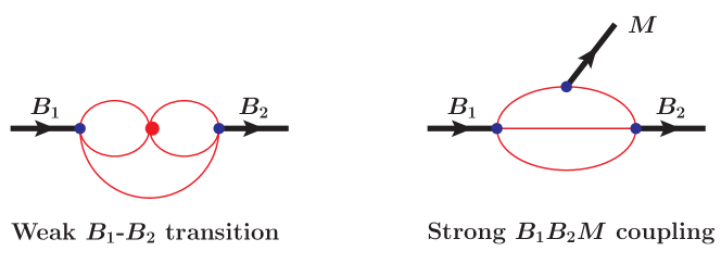
Figure 4: Feynman diagrams describing the building blocks of the LD-contributions

First, we discuss the matrix elements corresponding to the SD-contributions. One has

$$M_{\rm SD}(\Xi^{0}_{c}\to\Lambda_{c}^{+}\pi^{-}) = \frac{G_{F}}{\sqrt{2}}\Big{\{}V_{\rm CKM}^{(u)}\,\bar{u}(p_{2})\Big{[}(C_{2}^{(u)}+\xi C_{1}^{(u)})\,D_{\rm Ia}+(C_{2}^{(u)}-C_{1}^{(u)})\,D_{\rm IIb}\Big{]}u(p_{1})$$ (9)

$$\phantom{\frac{G_{F}}{\sqrt{2}}}+V_{\rm CKM}^{(c)}(C_{2}^{(c)}-C_{1}^{(c)})\,\bar{u}(p_{2})\Big{[}D_{\rm IIa}+D_{\rm III}\Big{]}u(p_{1})\Big{\}}\,.$$

Here, the factor $\xi=1/N_{c}$ where $N_{c}$ is the number of colors. This factor is set to zero in the numerical calculations according to the widely accepted phenomenology of the nonleptonic decays.

The contribution from the tree diagram factorizes into two pieces

$$D_{\rm Ia} = N_{c}\,g_{M}\int\!\!\frac{d^{4}k}{(2\pi)^{4}i}\widetilde{\Phi}_{M}(-k^{2})\,\mbox{\rm{tr}}\left[O^{\mu}_{L}S_{u}(k-w_{u}q)\gamma_{5}S_{d}(k+w_{d}q)\right]$$ (10)

$$\times 6\,g_{B_{1}}g_{B_{2}}\int\!\!\frac{d^{4}k_{1}}{(2\pi)^{4}i}\int\!\!\frac{d^{4}k_{2}}{(2\pi)^{4}i}\widetilde{\Phi}_{B_{1}}\Big{(}-\vec{\Omega}_{q}^{\,2}\Big{)}\widetilde{\Phi}_{B_{2}}\Big{(}-\vec{\Omega}_{r}^{\,2}\Big{)}$$

$$\times S_{c}(k_{2})\mbox{\rm{tr}}\left[S_{u}(k_{1}+p_{2})O_{\mu\,L}S_{s}(k_{1}+p_{1})\gamma_{5}S_{d}(k_{1}+k_{2})\gamma_{5}\right]$$

$$= -6f_{M}q^{\mu}g_{B_{1}}g_{B_{2}}\int\!\!\frac{d^{4}k_{1}}{(2\pi)^{4}i}\int\!\!\frac{d^{4}k_{2}}{(2\pi)^{4}i}\widetilde{\Phi}_{B_{1}}\Big{(}-\vec{\Omega}_{q}^{\,2}\Big{)}\widetilde{\Phi}_{B_{2}}\Big{(}-\vec{\Omega}_{r}^{\,2}\Big{)}$$

$$\times S_{c}(k_{2})\mbox{\rm{tr}}\left[S_{u}(k_{1}+p_{2})O_{\mu\,L}S_{s}(k_{1}+p_{1})\gamma_{5}S_{d}(k_{1}+k_{2})\gamma_{5}\right]$$

where $q_{1}=k_{2}-w_{1}^{\rm in}p_{1}$, $q_{2}=-k_{1}-k_{2}-w_{2}^{\rm in}p_{1}$ and $r_{1}=-k_{2}+w_{1}^{\rm out}p_{2}$, $r_{2}=-k_{1}-p_{2}+w_{2}^{\rm out}p_{2}$. The expression for $\vec{\Omega}^{\,2}$ is given by Eq. (8). Hereafter we adopt the brief notations $B_{1}$ for the ingoing baryon with the momentum $p_{1}$, $B_{2}$ for the outgoing baryon with the momentum $p_{2}$ and $M$ for the outgoing meson with the momentum $q$. The minus sign in front of $f_{M}$ appears because the momentum $q$ flows in the opposite direction from the decay of $M$-meson.

The calculation of the three-loop $W$–exchange diagrams is much more involved because the matrix element does not factorize. One has

$$D_{\rm IIb} = 12g_{B_{1}}g_{B_{2}}g_{M}\Big{[}\prod\limits_{i=1}^{3}\int\!\!\frac{d^{4}k_{i}}{(2\pi)^{4}i}\Big{]}\widetilde{\Phi}_{B_{1}}\Big{(}-\vec{\Omega}_{q}^{\,2}\Big{)}\widetilde{\Phi}_{B_{2}}\Big{(}-\vec{\Omega}_{r}^{\,2}\Big{)}\widetilde{\Phi}_{M}(-P^{2})\,$$ (11)

$$\times S_{c}(k_{3})\mbox{\rm{tr}}\left[\gamma_{5}S_{d}(k_{2}+p_{2})(1+\gamma_{5})S_{u}(k_{2}+k_{3})\right]$$

$$\times \mbox{\rm{tr}}\left[S_{u}(k_{1}+p_{2})\gamma_{5}S_{d}(k_{1}+p_{1})\gamma_{5}S_{s}(k_{1}+k_{3})(1-\gamma_{5})\right],$$

$$q_{1}=k_{3}-w_{1}^{\rm in}p_{1},\quad q_{2}=k_{1}+p_{1}-w_{2}^{\rm in}p_{1},$$

$$r_{1}=-k_{3}+w_{1}^{\rm out}p_{2},\quad r_{2}=k_{2}+k_{3}+w_{2}^{\rm out}p_{2},\qquad P=k_{1}+w_{u}p_{1}+w_{d}p_{2}.$$

$$D_{\rm IIa} = 6g_{B_{1}}g_{B_{2}}g_{M}\Big{[}\prod\limits_{i=1}^{3}\int\!\!\frac{d^{4}k_{i}}{(2\pi)^{4}i}\Big{]}\widetilde{\Phi}_{B_{1}}\Big{(}-\vec{\Omega}_{q}^{\,2}\Big{)}\widetilde{\Phi}_{B_{2}}\Big{(}-\vec{\Omega}_{r}^{\,2}\Big{)}\widetilde{\Phi}_{M}(-P^{2})\,$$ (12)

$$\times S_{c}(k_{3}-k_{2})O^{\mu}_{L}S_{c}(k_{1}+p_{1})\mbox{\rm{tr}}\left[S_{d}(k_{3})\gamma_{5}S_{u}(k_{2}+p_{2})\gamma_{5}S_{d}(k_{2}+p_{1})O_{\mu\,L}S_{s}(k_{3}-k_{1})\gamma_{5}\right]$$

$$q_{1}=k_{1}+p_{1}-w_{1}^{\rm in}p_{1},\quad q_{2}=-k_{3}-w_{2}^{\rm in}p_{1},$$

$$r_{1}=k_{2}-k_{3}+w_{1}^{\rm out}p_{2},\quad r_{2}=-k_{2}-p_{2}+w_{2}^{\rm out}p_{2},\qquad P=k_{2}+w_{u}p_{1}+w_{d}p_{2}.$$

$$D_{\rm III} = 6g_{B_{1}}g_{B_{2}}g_{M}\Big{[}\prod\limits_{i=1}^{3}\int\!\!\frac{d^{4}k_{i}}{(2\pi)^{4}i}\Big{]}\widetilde{\Phi}_{B_{1}}\Big{(}-\vec{\Omega}_{q}^{\,2}\Big{)}\widetilde{\Phi}_{B_{2}}\Big{(}-\vec{\Omega}_{r}^{\,2}\Big{)}\widetilde{\Phi}_{M}(-P^{2})\,$$ (13)

$$\times S_{c}(k_{3})O^{\mu}_{L}S_{c}(k_{2})\mbox{\rm{tr}}\left[S_{d}(k_{1}+k_{3})\gamma_{5}S_{u}(k_{1}+p_{2})\gamma_{5}S_{d}(k_{1}+p_{1})\gamma_{5}S_{s}(k_{1}+k_{2})O_{\mu\,R}\right]$$

$$q_{1}=k_{2}-w_{1}^{\rm in}p_{1},\quad q_{2}=k_{1}+p_{1}-w_{2}^{\rm in}p_{1},$$

$$r_{1}=-k_{3}+w_{1}^{\rm out}p_{2},\quad r_{2}=-k_{1}-p_{2}+w_{2}^{\rm out}p_{2},\qquad P=k_{1}+w_{u}p_{1}+w_{d}p_{2}.$$

The calculation of the three-loop integrals proceeds in two steps, first, one has to perform the loop integration by using Fock-Schwinger representation for the quark propagators and Gaussian form for the vertex functions. This allows one to do tensor loop integrals in a very efficient way since one can convert loop momenta into derivatives of the exponent function. The calculations are done by using a FORM code which works for any numbers of loops and propagators. Second, one has to calculate the obtained integrals numerically over Fock-Schwinger variables by adopting the quark confinement anzatz. The numerical calculations are done by using the FORTRAN codes which include the output from the FORM code written in the format of double precision accuracy. Since the files with the output from FORM contain several thousand lines we are unable to show them in the paper. The details of such calculations may be found in our recent papers Gutsche:2017hux ; Gutsche:2018utw . The calculation is quite time consuming both analytically and numerically.

Finally, the matrix element describing the SD-contributions are written as

$$M_{\rm SD}(\Xi^{0}_{c}\to\Lambda_{c}^{+}\pi^{-})=\frac{G_{F}}{\sqrt{2}}\bar{u}(p_{2})\Big{(}A_{\rm\,SD}+\gamma_{5}B_{\rm\,SD}\Big{)}u(p_{1}),$$ (14)

where

$$A_{\rm\,SD} = V_{\rm CKM}^{(u)}\Big{[}(C_{2}^{(u)}+\xi C_{1}^{(u)})a_{\rm Ia}+(C_{2}^{(u)}-C_{1}^{(u)})a_{\rm IIb}\Big{]}+V_{\rm CKM}^{(c)}(C_{2}^{(c)}-C_{1}^{(c)})\Big{(}a_{\rm IIa}+a_{\rm III}\Big{)},$$

$$B_{\rm\,SD} = V_{\rm CKM}^{(u)}\Big{[}(C_{2}^{(u)}+\xi C_{1}^{(u)})\,b_{\rm Ia}+(C_{2}^{(u)}-C_{1}^{(u)})\,b_{\rm IIb}\Big{]}+V_{\rm CKM}^{(c)}(C_{2}^{(c)}-C_{1}^{(c)})\Big{(}b_{\rm IIa}+b_{\rm III}\Big{)}.$$

Now, we discuss the matrix elements corresponding to the LD contributions. The contribution coming from the pole diagram in Fig. 2 with the $\Sigma^{0}_{c}$-resonance is written as

$$M_{\,\Sigma^{0}_{c}}=\frac{G_{F}}{\sqrt{2}}V_{\rm CKM}^{(c)}\left(C_{1}^{(c)}-C_{2}^{(c)}\right)\bar{u}(p_{2})D_{\,\Sigma^{0}_{c}\,\Lambda_{c}^{+}\,\pi^{-}}(p_{1},p_{2})S_{\,\Sigma^{0}_{c}}(p_{1})D_{\,\Xi^{0}_{c}\,\Sigma^{0}_{c}}(p_{1})u(p_{1})$$ (15)

where $S_{\,\Sigma^{0}_{c}}(p_{1})=1/(m_{\Sigma^{0}_{c}}-\not\!{p}_{1})$. The explicit form of $D$-functions are written down as

$$D_{\,\Sigma^{0}_{c}\,\Lambda_{c}^{+}\,\pi^{-}} = 12\,g_{\,\Sigma^{0}_{c}}\,g_{\,\Lambda_{c}^{+}}\,g_{\,\pi^{-}}\Big{[}\prod\limits_{i=1}^{2}\int\!\!\frac{d^{4}k_{i}}{(2\pi)^{4}i}\Big{]}\widetilde{\Phi}_{\,\Sigma^{0}_{c}}\Big{(}-\vec{\Omega}_{q}^{\,2}\Big{)}\widetilde{\Phi}_{\,\Lambda_{c}^{+}}\Big{(}-\vec{\Omega}_{r}^{\,2}\Big{)}\widetilde{\Phi}_{\,\pi^{-}}(-P^{2})\,$$ (16)

$$\times S_{c}(k_{2})\gamma_{\alpha}\gamma_{5}\,\mbox{\rm{tr}}\left[\gamma_{5}S_{u}(k_{1}+p_{2})\gamma_{5}S_{d}(k_{1}+p_{1})\gamma^{\alpha}S_{d}(k_{1}+k_{2})\right]$$

where $q_{1}=k_{2}-w_{1}^{\rm res}p_{1},q_{2}=-k_{1}-k_{2}-w_{2}^{\rm res}p_{1}$, $r_{1}=-k_{2}+w_{1}^{\rm out}p_{2},r_{2}=-k_{1}-(1-w_{2}^{\rm out})p_{2},$ and $P=k_{1}+w_{1}^{M}p_{1}+w_{2}^{M}p_{2}$. Here the notations are ${\rm``res^{\prime\prime}}=\Sigma^{0}_{c}$, ${\rm``out^{\prime\prime}}=\Lambda_{c}^{+}$ and $M=\pi^{-}$.

$$D_{\,\Xi^{0}_{c}\,\Sigma^{0}_{c}} = 12\,g_{\,\Xi^{0}_{c}}\,g_{\,\Sigma^{0}_{c}}\Big{[}\prod\limits_{i=1}^{3}\int\!\!\frac{d^{4}k_{i}}{(2\pi)^{4}i}\Big{]}\widetilde{\Phi}_{\,\Xi^{0}_{c}}\Big{(}-\vec{\Omega}_{q}^{\,2}\Big{)}\widetilde{\Phi}_{\,\Sigma^{0}_{c}}\Big{(}-\vec{\Omega}_{r}^{\,2}\Big{)}$$ (17)

$$\times \gamma_{\alpha}\gamma_{5}S_{c}(k_{2}+p_{1})O_{\mu\,L}S_{c}(k_{1}+p_{1})\,\mbox{\rm{tr}}\left[S_{d}(k_{3})\gamma^{\alpha}S_{d}(k_{3}-k_{2})O^{\mu}_{L}S_{s}(k_{3}-k_{1})\gamma_{5}\right]$$

where $q_{1}=k_{1}+(1-w_{1}^{\rm in})p_{1},\,q_{2}=-k_{3}-w_{2}^{\rm in}p_{1}$, $r_{1}=-k_{2}-(1-w_{1}^{\rm res})p_{1},\,r_{2}=k_{3}+w_{2}^{\rm res}p_{1}$ and ${\rm``in^{\prime\prime}}=\Xi^{0}_{c}$.

By using the mass-shell conditions, one obtains

$$\bar{u}(p_{2})D_{\,\Sigma^{0}_{c}\,\Lambda_{c}^{+}\,\pi^{-}}(p_{1},p_{2}) = \bar{u}(p_{2})\gamma_{5}(g^{(0)}_{\,\Sigma^{0}_{c}\,\Lambda_{c}^{+}\,\pi^{-}}+\not\!{p}_{1}\,g^{(1)}_{\,\Sigma^{0}_{c}\,\Lambda_{c}^{+}\,\pi^{-}}),$$

$$D_{\,\Xi^{0}_{c}\,\Sigma^{0}_{c}}(p_{1})u(p_{1}) = (a_{\,\Xi^{0}_{c}\,\Sigma^{0}_{c}}+\gamma_{5}\,b_{\,\Xi^{0}_{c}\,\Sigma^{0}_{c}})u(p_{1}).$$ (18)

The final expression for the $\Sigma^{0}_{c}$-resonance diagram is written as

$$M_{\Sigma^{0}_{c}}=\frac{G_{F}}{\sqrt{2}}\,\bar{u}(p_{2})\Big{(}A_{\Sigma^{0}_{c}}+\gamma_{5}\,B_{\Sigma^{0}_{c}}\Big{)}u(p_{1}),$$ (19)

where

$$A_{\Sigma^{0}_{c}} = V_{\rm CKM}^{(c)}\,\left(C_{1}^{(c)}-C_{2}^{(c)}\right)\,\frac{g^{(-)}_{\,\Sigma^{0}_{c}\,\Lambda_{c}^{+}\,\pi^{-}}b_{\,\Xi^{0}_{c}\,\Sigma^{0}_{c}}}{m_{\Sigma^{0}_{c}}+m_{\Xi^{0}_{c}}},\,\,\,\text{where}\,\,\,g^{(-)}_{\,\Sigma^{0}_{c}\,\Lambda_{c}^{+}\,\pi^{-}}=g^{(0)}_{\,\Sigma^{0}_{c}\,\Lambda_{c}^{+}\,\pi^{-}}-m_{\Xi^{0}_{c}}\,g^{(1)}_{\,\Sigma^{0}_{c}\,\Lambda_{c}^{+}\,\pi^{-}},$$

$$B_{\Sigma^{0}_{c}} = V_{\rm CKM}^{(c)}\,\left(C_{1}^{(c)}-C_{2}^{(c)}\right)\,\frac{g^{(+)}_{\,\Sigma^{0}_{c}\,\Lambda_{c}^{+}\,\pi^{-}}a_{\,\Xi^{0}_{c}\,\Sigma^{0}_{c}}}{m_{\Sigma^{0}_{c}}-m_{\Xi^{0}_{c}}},\,\,\,\text{where}\,\,\,g^{(+)}_{\,\Sigma^{0}_{c}\,\Lambda_{c}^{+}\,\pi^{-}}=g^{(0)}_{\,\Sigma^{0}_{c}\,\Lambda_{c}^{+}\,\pi^{-}}+m_{\Xi^{0}_{c}}\,g^{(1)}_{\,\Sigma^{0}_{c}\,\Lambda_{c}^{+}\,\pi^{-}}.$$

The matrix elements corresponding to the LD-contributions coming from the second diagram in Fig. 2 with $B_{\rm res}=\Xi^{+}_{c},\Xi^{{}^{\prime}\,+}_{c}$ are calculated in a similar way. We perform the necessary steps below.

$$M_{\Xi^{{}^{\prime}\,+}_{c}} = \frac{G_{F}}{\sqrt{2}}\,\bar{u}(p_{2})\Big{\{}\left[V_{\rm CKM}^{(u)}\left(C_{1}^{(u)}-C_{2}^{(u)}\right)D^{(u)}_{\,\Xi^{{}^{\prime}\,+}_{c}\,\Lambda^{+}_{c}}(p_{2})+V_{\rm CKM}^{(c)}\left(C_{1}^{(c)}-C_{2}^{(c)}\right)D^{(c)}_{\,\Xi^{{}^{\prime}\,+}_{c}\,\Lambda^{+}_{c}}(p_{2})\right]$$ (20)

$$\phantom{\frac{G_{F}}{\sqrt{2}}\,\bar{u}(p_{2})}\times S_{\,\Xi^{{}^{\prime}\,+}_{c}}(p_{2})D_{\,\Xi^{0}_{c}\,\Xi^{{}^{\prime}\,+}_{c}\,\pi^{-}}(p_{1},p_{2})\Big{\}}\,u(p_{1})$$

where

$$D^{(u)}_{\,\Xi^{{}^{\prime}\,+}_{c}\,\Lambda^{+}_{c}}(p_{2}) = -12\,g_{\,\Xi^{{}^{\prime}\,+}_{c}}\,g_{\,\Lambda^{+}_{c}}\Big{[}\prod\limits_{i=1}^{3}\int\!\!\frac{d^{4}k_{i}}{(2\pi)^{4}i}\Big{]}\widetilde{\Phi}_{\,\Xi^{{}^{\prime}\,+}_{c}}\Big{(}-\vec{\Omega}_{q}^{\,2}\Big{)}\widetilde{\Phi}_{\,\Lambda^{+}_{c}}\Big{(}-\vec{\Omega}_{r}^{\,2}\Big{)}$$ (21)

$$\times S_{c}(k_{3})\gamma_{\alpha}\gamma_{5}\mbox{\rm{tr}}\left[S_{u}(k_{2}+p_{2})(1+\gamma_{5})S_{d}(k_{2}+k_{3})\gamma_{5}\right]$$

$$\times \mbox{\rm{tr}}\left[S_{u}(k_{1}+p_{2})\gamma^{\alpha}S_{s}(k_{1}+k_{3})(1-\gamma_{5})\right]$$

where $q_{1}=k_{3}-w_{1}^{\rm res}p_{2},\,q_{2}=k_{1}+(1-w_{2}^{\rm res})p_{2}$, $r_{1}=-k_{3}+w_{1}^{\rm out}p_{2},\,r_{2}=-k_{2}-(1-w_{2}^{\rm out})p_{2}$ and ${\rm``res^{\prime\prime}}=\Xi^{{}^{\prime}\,+}_{c}$, ${\rm``out^{\prime\prime}}=\Lambda^{+}_{c}$.

$$D^{(c)}_{\,\Xi^{{}^{\prime}\,+}_{c}\,\Lambda^{+}_{c}}(p_{2}) = -6\,g_{\,\Xi^{{}^{\prime}\,+}_{c}}\,g_{\,\Lambda^{+}_{c}}\Big{[}\prod\limits_{i=1}^{3}\int\!\!\frac{d^{4}k_{i}}{(2\pi)^{4}i}\Big{]}\widetilde{\Phi}_{\,\Xi^{{}^{\prime}\,+}_{c}}\Big{(}-\vec{\Omega}_{q}^{\,2}\Big{)}\widetilde{\Phi}_{\,\Lambda^{+}_{c}}\Big{(}-\vec{\Omega}_{r}^{\,2}\Big{)}$$ (22)

$$\times S_{c}(k_{2}+p_{2})O_{\mu\,L}S_{c}(k_{1}+p_{2})\,\gamma_{\alpha}\gamma_{5}$$

$$\times \mbox{\rm{tr}}\left[S_{u}(k_{3})\gamma_{5}S_{d}(k_{3}-k_{2})O_{L}^{\mu}S_{s}(k_{3}-k_{1})\gamma^{\alpha}\right]$$

where $q_{1}=k_{1}+(1-w_{1}^{\rm res})p_{2},\,q_{2}=-k_{3}-w_{2}^{\rm res}p_{2}$, $r_{1}=-k_{2}-(1-w_{1}^{\rm out})p_{2},\,r_{2}=k_{3}+w_{2}^{\rm out}p_{2}$.

$$D_{\,\Xi_{c}^{0}\,\Xi^{{}^{\prime}\,+}_{c}\,\pi^{-}} = -6\,g_{\,\Xi_{c}^{0}}\,g_{\,\Xi^{{}^{\prime}\,+}_{c}}\,g_{\,\pi^{-}}\Big{[}\prod\limits_{i=1}^{2}\int\!\!\frac{d^{4}k_{i}}{(2\pi)^{4}i}\Big{]}\widetilde{\Phi}_{\,\Xi_{c}^{0}}\Big{(}-\vec{\Omega}_{q}^{\,2}\Big{)}\widetilde{\Phi}_{\,\Xi^{{}^{\prime}\,+}_{c}}\Big{(}-\vec{\Omega}_{r}^{\,2}\Big{)}\widetilde{\Phi}_{\,\pi^{-}}(-P^{2})\,$$ (23)

$$\times \gamma_{\alpha}\gamma_{5}\,S_{c}(k_{2})\mbox{\rm{tr}}\left[S_{u}(k_{1}+p_{2})\gamma_{5}S_{d}(k_{1}+p_{1})\gamma_{5}S_{s}(k_{1}+k_{2})\gamma^{\alpha}\right]$$

where $q_{1}=k_{2}-w_{1}^{\rm in}p_{1},\,q_{2}=k_{1}+(1-w_{2}^{\rm in})p_{1}$, $r_{1}=-k_{2}+w_{1}^{\rm res}p_{2},\quad r_{2}=-k_{1}-(1-w_{2}^{\rm res})p_{2}$, $P=k_{1}+w_{1}^{M}p_{1}+w_{2}^{M}p_{2}$ and ${\rm``in^{\prime\prime}}=\Xi^{0}_{c}$. By using the mass-shell conditions, one obtains

$$\bar{u}(p_{2})D^{(u,c)}_{\,\Xi^{{}^{\prime}\,+}_{c}\,\Lambda^{+}_{c}}(p_{2}) = \bar{u}(p_{2})\left(a^{(u,c)}_{\,\Xi^{{}^{\prime}\,+}_{c}\,\Lambda^{+}_{c}}+\gamma_{5}\,b^{(u,c)}_{\,\Xi^{{}^{\prime}\,+}_{c}\,\Lambda^{+}_{c}}\right)$$

$$D_{\,\Xi^{0}_{c}\,\Xi^{{}^{\prime}\,+}_{c}\,\pi^{-}}(p_{1},p_{2})u(p_{1}) = \gamma_{5}\left(g^{(0)}_{\,\Xi^{0}_{c}\,\Xi^{{}^{\prime}\,+}_{c}\,\pi^{-}}+\not\!{p}_{2}g^{(1)}_{\,\Xi^{0}_{c}\,\Xi^{{}^{\prime}\,+}_{c}\,\pi^{-}}\right)u(p_{1}).$$

The final expression for the second pole diagram is written as

$$M_{\Xi_{c}^{{}^{\prime}\,+}}=\frac{G_{F}}{\sqrt{2}}\,\bar{u}(p_{2})\Big{(}A_{\Xi_{c}^{{}^{\prime}\,+}}+\gamma_{5}\,B_{\Xi_{c}^{{}^{\prime}\,+}}\Big{)}u(p_{1}),$$ (24)

where

$$A_{\Xi_{c}^{{}^{\prime}\,+}} = \Big{\{}V_{\rm CKM}^{(u)}\,\left(C_{1}^{(u)}-C_{2}^{(u)}\right)\,b^{(u)}_{\,\Xi_{c}^{{}^{\prime}\,+}\,\Lambda^{+}_{c}}+V_{\rm CKM}^{(c)}\,\left(C_{1}^{(c)}-C_{2}^{(c)}\right)\,b^{(c)}_{\,\Xi_{c}^{{}^{\prime}\,+}\,\Lambda^{+}_{c}}\Big{\}}\frac{g^{(+)}_{\,\Xi^{0}_{c}\,\Xi^{{}^{\prime}\,+}_{c}\,\pi^{-}}}{m_{\,\Xi_{c}^{{}^{\prime}\,+}}+m_{\,\Lambda^{+}_{c}}},$$

$$B_{\Xi_{c}^{{}^{\prime}\,+}} = \Big{\{}V_{\rm CKM}^{(u)}\,\left(C_{1}^{(u)}-C_{2}^{(u)}\right)\,a^{(u)}_{\,\Xi_{c}^{{}^{\prime}\,+}\,\Lambda^{+}_{c}}+V_{\rm CKM}^{(c)}\,\left(C_{1}^{(c)}-C_{2}^{(c)}\right)\,a^{(c)}_{\,\Xi_{c}^{{}^{\prime}\,+}\,\Lambda^{+}_{c}}\Big{\}}\frac{g^{(-)}_{\,\Xi^{0}_{c}\,\Xi^{{}^{\prime}\,+}_{c}\,\pi^{-}}}{m_{\,\Xi_{c}^{{}^{\prime}\,+}}-m_{\,\Lambda^{+}_{c}}},$$

where $g^{(\pm)}_{\,\Xi^{0}_{c}\,\Xi^{{}^{\prime}\,+}_{c}\,\pi^{-}}=g^{(0)}_{\,\Xi^{0}_{c}\,\Xi^{{}^{\prime}\,+}_{c}\,\pi^{-}}\pm m_{\Lambda_{c}^{+}}g^{(1)}_{\,\Xi^{0}_{c}\,\Xi^{{}^{\prime}\,+}_{c}\,\pi^{-}}$.

$$M_{\Xi^{+}_{c}} = \frac{G_{F}}{\sqrt{2}}\,\bar{u}(p_{2})\Big{\{}\left[V_{\rm CKM}^{(u)}\left(C_{2}^{(u)}-C_{1}^{(u)}\right)D^{(u)}_{\,\Xi^{+}_{c}\,\Lambda^{+}_{c}}(p_{2})+V_{\rm CKM}^{(c)}\left(C_{2}^{(c)}-C_{1}^{(c)}\right)D^{(c)}_{\,\Xi^{+}_{c}\,\Lambda^{+}_{c}}(p_{2})\right]$$ (25)

$$\phantom{\frac{G_{F}}{\sqrt{2}}\,\bar{u}(p_{2})}\times S_{\,\Xi^{+}_{c}}(p_{2})D_{\,\Xi^{0}_{c}\,\Xi^{+}_{c}\,\pi^{-}}(p_{1},p_{2})\Big{\}}\,u(p_{1})$$

where

$$D^{(u)}_{\,\Xi^{+}_{c}\,\Lambda^{+}_{c}}(p_{2}) = 12\,g_{\,\Xi^{+}_{c}}\,g_{\,\Lambda^{+}_{c}}\Big{[}\prod\limits_{i=1}^{3}\int\!\!\frac{d^{4}k_{i}}{(2\pi)^{4}i}\Big{]}\widetilde{\Phi}_{\,\Xi^{+}_{c}}\Big{(}-\vec{\Omega}_{q}^{\,2}\Big{)}\widetilde{\Phi}_{\,\Lambda^{+}_{c}}\Big{(}-\vec{\Omega}_{r}^{\,2}\Big{)}$$ (26)

$$\times S_{c}(k_{3})\mbox{\rm{tr}}\left[S_{u}(k_{2}+p_{2})(1+\gamma_{5})S_{d}(k_{2}+k_{3})\gamma_{5}\right]$$

$$\times \mbox{\rm{tr}}\left[S_{u}(k_{1}+p_{2})\gamma_{5}S_{s}(k_{1}+k_{3})(1-\gamma_{5})\right]$$

where $q_{1}=k_{3}-w_{1}^{\rm res}p_{2},\,q_{2}=k_{1}+(1-w_{2}^{\rm res})p_{2}$, $r_{1}=-k_{3}+w_{1}^{\rm out}p_{2},\,r_{2}=-k_{2}-(1-w_{2}^{\rm out})p_{2}$ and ${\rm``res^{\prime\prime}}=\Xi^{+}_{c}$, ${\rm``out^{\prime\prime}}=\Lambda^{+}_{c}$.

$$D^{(c)}_{\,\Xi^{+}_{c}\,\Lambda^{+}_{c}}(p_{2}) = -6\,g_{\,\Xi^{+}_{c}}\,g_{\,\Lambda^{+}_{c}}\Big{[}\prod\limits_{i=1}^{3}\int\!\!\frac{d^{4}k_{i}}{(2\pi)^{4}i}\Big{]}\widetilde{\Phi}_{\,\Xi^{+}_{c}}\Big{(}-\vec{\Omega}_{q}^{\,2}\Big{)}\widetilde{\Phi}_{\,\Lambda^{+}_{c}}\Big{(}-\vec{\Omega}_{r}^{\,2}\Big{)}$$ (27)

$$\times S_{c}(k_{2}+p_{2})O_{\mu\,L}S_{c}(k_{1}+p_{2})$$

$$\times \mbox{\rm{tr}}\left[S_{u}(k_{3})\gamma_{5}S_{d}(k_{3}-k_{2})O_{L}^{\mu}S_{s}(k_{3}-k_{1})\gamma_{5}\right]$$

where $q_{1}=k_{1}+(1-w_{1}^{\rm res})p_{2},\,q_{2}=-k_{3}-w_{2}^{\rm res}p_{2}$, $r_{1}=-k_{2}-(1-w_{1}^{\rm out})p_{2},\,r_{2}=k_{3}+w_{2}^{\rm out}p_{2}$. By using the mass-shell conditions, one obtains

$$\bar{u}(p_{2})D^{(u,c)}_{\,\Xi^{+}_{c}\,\Lambda^{+}_{c}}(p_{2}) = \bar{u}(p_{2})\left(a^{(u,c)}_{\,\Xi^{+}_{c}\,\Lambda^{+}_{c}}+\gamma_{5}\,b^{(u,c)}_{\,\Xi^{+}_{c}\,\Lambda^{+}_{c}}\right)$$ (28)

It appears that the strong transition $\Xi_{c}^{0}\to\Xi^{+}_{c}+\pi^{-}$ is identically equal to zero due to the chosen form of the interpolating quark current as shown in Table 1: $\epsilon^{abc}c^{a}(u^{b}C\gamma_{5}s^{c})$. As a result, this transition is described by the diagram which contains the trace of a string with three quark propagators and three $\gamma_{5}$ matrices that gives zero contribution. Explicitly we have

$$D_{\,\Xi_{c}^{0}\,\Xi^{+}_{c}\,\pi^{-}} = 6\,g_{\,\Xi_{c}^{0}}\,g_{\,\Xi^{+}_{c}}\,g_{\,\pi^{-}}\Big{[}\prod\limits_{i=1}^{2}\int\!\!\frac{d^{4}k_{i}}{(2\pi)^{4}i}\Big{]}\widetilde{\Phi}_{\,\Xi_{c}^{0}}\Big{(}-\vec{\Omega}_{q}^{\,2}\Big{)}\widetilde{\Phi}_{\,\Xi^{+}_{c}}\Big{(}-\vec{\Omega}_{r}^{\,2}\Big{)}\widetilde{\Phi}_{\,\pi^{-}}(-P^{2})\,$$ (29)

$$\times S_{c}(k_{2})\mbox{\rm{tr}}\left[S_{u}(k_{1}+p_{2})\gamma_{5}S_{d}(k_{1}+p_{1})\gamma_{5}S_{s}(k_{1}+k_{2})\gamma_{5}\right]\equiv 0.$$

In Ref. Cheng:1992ff it was shown that the vanishing strong couping for $\Xi_{c}^{0}\to\Xi^{+}_{c}\,\pi^{-}$ transition is a consequence of heavy quark and chiral symmetries. Hence it is a model-independent statement. Here, one has to comment that there are two kinds of the interpolating currents for the $\Lambda$-type baryons $(\Lambda_{Q},\Xi_{Q})$ where $Q=b,c$. They are written as $\epsilon^{abc}Q^{a}(u^{b}C\gamma_{5}s^{c})$ (scalar diquark) and $\epsilon^{abc}\gamma_{\alpha}Q^{a}(u^{b}C\gamma^{\alpha}\gamma_{5}s^{c})$ (vector diquark). For the details, see Refs Shuryak:1981fza ; Grozin:1992td ; Groote:1996xb ; Ivanov:1996fj .

It is widely accepted that S-wave amplitude is saturated by the $1/2^{-}$ resonances, see, e.g., Refs Marshak ; Bailin:1977gv for the original suggestions and Ebert:1983yh ; Ebert:1983ih ; Cheng:1985dw ; Cheng:2018hwl for the subsiquent applications. Ordinarily, their contributions are calculated by using the well-known soft-pion theorem in the current-algebra approach. It allows one to express the parity-violating S-wave amplitude in terms of parity-conserving matrix elements. In our case, one has

$$A_{1/2^{-}}\left(\Xi_{c}^{0}\to\Lambda_{c}^{+}+\pi^{-}\right) = \frac{1}{f_{\pi}}A_{\Xi^{+}_{c}\Lambda_{c}^{+}},$$

$$A_{\Xi^{+}_{c}\Lambda_{c}^{+}} = V_{\rm CKM}^{(u)}\left(C_{2}^{(u)}-C_{1}^{(u)}\right)a^{(u)}_{\,\Xi^{+}_{c}\,\Lambda^{+}_{c}}+V_{\rm CKM}^{(c)}\left(C_{2}^{(c)}-C_{1}^{(c)}\right)a^{(c)}_{\,\Xi^{+}_{c}\,\Lambda^{+}_{c}}.$$ (30)

The quantities $a^{(u,c)}_{\,\Xi^{+}_{c}\,\Lambda^{+}_{c}}$ and $b^{(u,c)}_{\,\Xi^{+}_{c}\,\Lambda^{+}_{c}}$ are defined by Eqs. (26)-(28).

Finally, the transition $\Xi_{c}^{0}\to\Lambda_{c}^{+}+\pi^{-}$ amplitude is written in terms of invariant amplitudes as

$$<\Lambda_{c}^{+}\,\pi^{-}|{\mathcal{H}}_{\rm eff}|\Xi_{c}^{0}>=\frac{G_{F}}{\sqrt{2}}\,\bar{u}(p_{2})\left(A+\gamma_{5}B\right)u(p_{1})$$ (31)

where $A$ and $B$ are given by

$$A = A_{\rm SD}+A_{\rm LD},\qquad A_{\rm LD}=A_{\Sigma^{0}_{c}}+A_{\Xi^{{}^{\prime}\,+}_{c}}+A_{1/2^{-}},$$

$$B = B_{\rm SD}+B_{\rm LD},\qquad B_{\rm LD}=B_{\Sigma^{0}_{c}}+B_{\Xi^{{}^{\prime}\,+}_{c}}.$$ (32)

It is more convenient to use helicity amplitudes $H_{\lambda_{1}\lambda_{M}}$ instead of invariant ones $A$ and $B$ as described in Korner:1992wi . One has

$$H^{V}_{\tfrac{1}{2}\,t}=\sqrt{Q_{+}}\,A\,,\qquad H^{A}_{\tfrac{1}{2}\,t}=\sqrt{Q_{-}}\,B\,,$$ (33)

where $m_{\pm}=m_{1}\pm m_{2}$, $Q_{\pm}=m_{\pm}^{2}-q^{2}$.

Finally, the two-body decay width reads

$$\Gamma(B_{1}\to B_{2}+M)=\frac{G_{F}^{2}}{32\pi}\frac{\mathbf{|p_{2}|}}{m_{1}^{2}}\,{\mathcal{H}}_{S}\,,\quad{\mathcal{H}}_{S}=2\Big{(}\Big{|}H^{V}_{\tfrac{1}{2}\,t}\Big{|}^{2}\,+\,\Big{|}H^{A}_{\tfrac{1}{2}\,t}\Big{|}^{2}\Big{)}\,$$ (34)

where $\mathbf{|p_{2}|}=\lambda^{1/2}(m_{1}^{2},m_{2}^{2},q^{2})/(2m_{1})$.

IV   Numerical results

Our covariant constituent quark model contains a number of model parameters which have been determined by a global fit to a multitude of decay processes. The values of the constituent quark masses $m_{q}$ are taken from the last fit in Gutsche:2015mxa . In the fit, the infrared cutoff parameter $\lambda$ of the model has been kept fixed as found in the original paper Branz:2009cd . Table 2 shows as below: The size parameters of light meson were fixed by fitting the data on the leptonic decay constant. The numerical values of the size parameters and the leptonic decay constants for pion is shown in Table 3.

Table 2: Constituent quark masses and infrared cutoff parameter $\lambda$.

$m_{u/d}$	$m_{s}$	$m_{c}$	$\lambda$
0.241	0.428	2.16	0.181	GeV

Table 3: Size parameter and leptonic decay constant of pion.

Meson	$\Lambda_{M}$ (GeV)	$f_{M}$ (MeV)	$f_{M}^{\rm expt}$ (MeV)
Pion	0.871	130.3	130.41 $\pm$ 0.20

Since the experimental data of the single charm baryon decays become to appear recently, we will assume for the time being that the size parameters of all single charm baryons are the same. In Fig. 5 we plot the dependence on this parameter denoted as $\Lambda_{c}$ of branching fractions $\Xi_{c}^{0}\to\Lambda_{c}^{+}+\pi^{-}$. One can see that the measured branching fraction can be accommodated in the framework of this work by having $\Lambda_{c}\approx 0.61$ GeV. In addition to the line describing the central value of the experimental data, we also display the strip corresponding to experimental uncertainties. In order to estimate the uncertainty caused by the choice of the size parameter we allow the size parameter to vary from $\Lambda_{c\,\rm min}=0.54$ to $\Lambda_{c\,\rm max}=0.66$ GeV that correspond to the intersections of the theoretical curve for branching fraction with the experimantal lower and upper error bars.

We evaluate the mean $\bar{\Gamma}=\sum_{i=1}^{N}\Gamma_{i}/N$ and the mean square deviation
$\sigma^{2}=\sum_{i=1}^{N}(\Gamma_{i}-\bar{\Gamma})^{2}/N$. Finally, our result for the branching fraction reads as

$${\mathcal{B}}\left(\Xi_{c}^{0}\to\Lambda_{c}^{+}+\pi^{-}\right)=(0.54\pm 0.11)\%$$ (35)

which should be compared with the data from LHCb and Belle: ${\mathcal{B}}=(0.55\pm 0.02\pm 0.18)\%$ LHCb:2020gge and ${\mathcal{B}}=(0.54\pm 0.05\pm 0.12)\%$ Belle:2022kqi .

For comparison, we plot in Fig. 5 both the separate SD-contributions coming from the diagrams with topologies Ia, IIa, IIb, and III and the LD-contributions coming from the pole diagrams. It is readily seen that the SD-contributions are much smaller than those coming from the pole LD-diagrams.

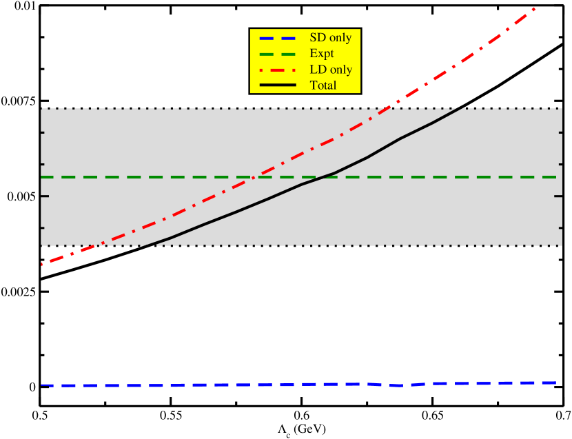
Figure 5: Dependence of the branching fractions on the size parameter.

The numerical results for the SD, LD and full amplitudes are shown in Table 4. One can see that $|A_{\rm LD}|>|A_{\rm SD}|$.

Table 4: SD, LD and full amplitudes in units of GeV².

Amplitudes	SD	LD	SD+LD
A-ampl.	0.0156	-0.0751	-0.0595
B-ampl.	0.166	-5.378	-5.212

Also it would be instructive to evaluate the asymmetry parameter defined by

$$\alpha=\frac{|H_{1/2\,t}|^{2}-|H_{-1/2\,t}|^{2}}{|H_{1/2\,t}|^{2}+|H_{-1/2\,t}|^{2}}=-\frac{2\kappa AB}{A^{2}+\kappa^{2}B^{2}},$$ (36)

where $\kappa=\bm{|{\rm p}_{2}|}/(E_{2}+m_{2})$ and $E_{2}=(m_{1}^{2}+m_{2}^{2}-q^{2})/(2m_{1})$. The numerical value of the asymmetry parameter is found to be equal to

$$\alpha=-0.751.$$ (37)

Finally, we compare our results obtained for the branching fraction and the asymmetry parameter with other the data and other approaches in Table 5.

Table 5: Comparison of our findings with other approaches.

Approach	BR($\Xi_{c}^{0}\to\Lambda^{+}_{c}\pi^{-}$)%	Asymmetry
Our model	$0.54\pm 0.11$	$-0.75$
LHCb LHCb:2020gge	$0.55\pm 0.02\pm 0.1$	$\ldots$
Belle Belle:2022kqi	$0.54\pm 0.05\pm 0.12$	$\ldots$
Voloshin Voloshin:2019ngb	$>0.025\pm 0.015$	$\ldots$
Gronau and Rosner Gronau:2016xiq (construc)	$0.194\pm 0.070$	$\ldots$
Gronau and Rosner Gronau:2016xiq (destruc)	$<0.01$	$\ldots$
Faller and Mannel Faller:2015oma	$<0.39$	$\ldots$
Cheng et al. Cheng:2022jbr	$0.72\pm 0.07$	$0.46\pm 0.05$
Niu et al. Niu:2021qcc	$0.58\pm 0.21$	$-0.16$

V   Summary and conclusion

We have studied two-body nonleptonic $\Delta C=0$ decay $\Xi^{0}_{c}\to\Lambda_{c}^{+}+\pi^{-}$ in the framework of the covariant confined quark model (CCQM) with account for both short and long distance effects. The short distance effects are induced by four topologies of external and internal weak $W$-interactions, while long distance effects are saturated by an inclusion of the so-called pole diagrams. Pole diagrams are generated by resonance contributions of the low-lying spin $\frac{1}{2}^{+}$ ($\Sigma_{c}^{0}$ and $\Xi_{c}^{\,\prime\,+}$) and spin $\frac{1}{2}^{-}$ baryons. The last contributions are calculated by using the well-known soft-pion theorem. It is found that the contribution of the SD diagrams is significantly suppressed, by more than one order of magnitude in comparison with data. The most significant contributions are coming from the intermediate $\frac{1}{2}^{+}$ and $\frac{1}{2}^{-}$ resonances. We can get consistency with the experimental data for the value of size parameter being equal to $\Lambda\approx 0.61$ GeV.

References

• (1) R. Aaij et al. [LHCb], Phys. Rev. D 102, no.7, 071101 (2020) [arXiv:2007.12096 [hep-ex]].
• (2) S. S. Tang et al. [Belle], Phys. Rev. D 107, no.3, 032005 (2023) [arXiv:2206.08527 [hep-ex]].
• (3) S. Groote and J. G. Körner, Eur. Phys. J. C 82, no.4, 297 (2022) [arXiv:2112.14599 [hep-ph]].
• (4) H. Y. Cheng, C. Y. Cheung, G. L. Lin, Y. C. Lin, T. M. Yan and H. L. Yu, Phys. Rev. D 46, 5060-5068 (1992)
• (5) M. B. Voloshin, Phys. Lett. B 476, 297-302 (2000) [arXiv:hep-ph/0001057 [hep-ph]].
• (6) M. B. Voloshin, Phys. Rev. D 100, no.11, 114030 (2019) [arXiv:1911.05730 [hep-ph]].
• (7) R. Aaij et al. [LHCb], Phys. Rev. D 100, no.3, 032001 (2019) [arXiv:1906.08350 [hep-ex]].
• (8) M. Gronau and J. L. Rosner, Phys. Lett. B 757, 330-333 (2016) [arXiv:1603.07309 [hep-ph]].
• (9) S. Faller and T. Mannel, Phys. Lett. B 750, 653-659 (2015) [arXiv:1503.06088 [hep-ph]].
• (10) H. Y. Cheng, C. Y. Cheung, G. L. Lin, Y. C. Lin, T. M. Yan and H. L. Yu, JHEP 03, 028 (2016) [arXiv:1512.01276 [hep-ph]].
• (11) H. Y. Cheng and F. Xu, Phys. Rev. D 105, no.9, 094011 (2022) [arXiv:2204.03149 [hep-ph]].
• (12) H. Y. Cheng, C. W. Liu and F. Xu, Phys. Rev. D 106, no.9, 093005 (2022) [arXiv:2209.00257 [hep-ph]].
• (13) P. Y. Niu, Q. Wang and Q. Zhao, Phys. Lett. B 826, 136916 (2022) [arXiv:2111.14111 [hep-ph]].
• (14) T. Branz, A. Faessler, T. Gutsche, M. A. Ivanov, J. G. Körner and V. E. Lyubovitskij, Phys. Rev. D 81, 034010 (2010) [arXiv:0912.3710 [hep-ph]].
• (15) T. Gutsche, M. A. Ivanov, J. G. Körner, V. E. Lyubovitskij and Z. Tyulemissov, Phys. Rev. D 99, no.5, 056013 (2019) [arXiv:1812.09212 [hep-ph]].
• (16) M. A. Ivanov, J. G. Körner, V. E. Lyubovitskij and Z. Tyulemissov, Phys. Rev. D 104, no.7, 074004 (2021) [arXiv:2107.08831 [hep-ph]].
• (17) T. Gutsche, M. A. Ivanov, J. G. Körner, V. E. Lyubovitskij, P. Santorelli and N. Habyl, Phys. Rev. D 91, no.7, 074001 (2015) [erratum: Phys. Rev. D 91, no.11, 119907 (2015)] [arXiv:1502.04864 [hep-ph]].
• (18) M. A. Ivanov, J. G. Körner and V. E. Lyubovitskij, Phys. Part. Nucl. 51, no.4, 678-685 (2020)
• (19) M. A. Ivanov, Particles 3, no.1, 123-144 (2020)
• (20) T. Gutsche, M. A. Ivanov, J. G. Körner, V. E. Lyubovitskij and Z. Tyulemissov, Phys. Rev. D 100, no.11, 114037 (2019) [arXiv:1911.10785 [hep-ph]].
• (21) T. Gutsche, M. A. Ivanov, J. G. Körner and V. E. Lyubovitskij, Particles 2, no.2, 339-356 (2019)
• (22) T. Gutsche, M. A. Ivanov, J. G. Körner and V. E. Lyubovitskij, Phys. Rev. D 98, no.7, 074011 (2018) [arXiv:1806.11549 [hep-ph]].
• (23) M. A. Ivanov, PoS EPS-HEP2017, 220 (2017) [arXiv:1711.10821 [hep-ph]].
• (24) T. Gutsche, M. A. Ivanov, J. G. Körner and V. E. Lyubovitskij, Phys. Rev. D 96, no.5, 054013 (2017) [arXiv:1708.00703 [hep-ph]].
• (25) T. Gutsche, M. A. Ivanov, J. G. Körner, V. E. Lyubovitskij, V. V. Lyubushkin and P. Santorelli, Phys. Rev. D 96, no.1, 013003 (2017) [arXiv:1705.07299 [hep-ph]].
• (26) T. Gutsche, M. A. Ivanov, J. G. Körner, V. E. Lyubovitskij and P. Santorelli, Phys. Rev. D 93, no.3, 034008 (2016) [arXiv:1512.02168 [hep-ph]].
• (27) T. Gutsche, M. A. Ivanov, J. G. Körner, V. E. Lyubovitskij and P. Santorelli, Phys. Rev. D 92, no.11, 114008 (2015) [arXiv:1510.02266 [hep-ph]].
• (28) N. Habyl, T. Gutsche, M. A. Ivanov, J. G. Körner, V. E. Lyubovitskij and P. Santorelli, Int. J. Mod. Phys. Conf. Ser. 39, 1560112 (2015) [arXiv:1509.07688 [hep-ph]].
• (29) T. Gutsche, M. A. Ivanov, J. G. Körner, V. E. Lyubovitskij and P. Santorelli, Phys. Rev. D 90, no.11, 114033 (2014) [erratum: Phys. Rev. D 94, no.5, 059902 (2016)] [arXiv:1410.6043 [hep-ph]].
• (30) T. Gutsche, M. A. Ivanov, J. G. Körner, V. E. Lyubovitskij and P. Santorelli, Phys. Rev. D 88, no.11, 114018 (2013) [arXiv:1309.7879 [hep-ph]].
• (31) T. Gutsche, M. A. Ivanov, J. G. Körner, V. E. Lyubovitskij and P. Santorelli, Phys. Rev. D 87, 074031 (2013) [arXiv:1301.3737 [hep-ph]].
• (32) T. Gutsche, M. A. Ivanov, J. G. Körner, V. E. Lyubovitskij and P. Santorelli, Phys. Rev. D 86, 074013 (2012) [arXiv:1207.7052 [hep-ph]].
• (33) A. De Rujula, H. Georgi and S. L. Glashow, Phys. Rev. D 12, 147-162 (1975)
• (34) J. G. Körner, M. Kramer and D. Pirjol, Prog. Part. Nucl. Phys. 33, 787-868 (1994) [arXiv:hep-ph/9406359 [hep-ph]].
• (35) R. L. Workman et al. [Particle Data Group], PTEP 2022, 083C01 (2022)
• (36) G. Buchalla, A. J. Buras and M. E. Lautenbacher, Rev. Mod. Phys. 68, 1125-1144 (1996) [arXiv:hep-ph/9512380 [hep-ph]].
• (37) A. Salam, Nuovo Cimento   25, 224 (1962).
• (38) S. Weinberg, Phys. Rev.  130, 776 (1963).
• (39) K. Hayashi, M. Hirayama, T. Muta, N. Seto, and T. Shirafuji, Fortsch. Phys. 15, 625 (1967).
• (40) G. V. Efimov and M. A. Ivanov, The Quark Confinement Model of Hadrons, (IOP Publishing, Bristol $\&$ Philadelphia, 1993)
• (41) E. V. Shuryak, Nucl. Phys. B 198, 83-101 (1982)
• (42) A. G. Grozin and O. I. Yakovlev, Phys. Lett. B 285, 254-262 (1992) [arXiv:hep-ph/9908364 [hep-ph]].
• (43) S. Groote, J. G. Körner and O. I. Yakovlev, Phys. Rev. D 54, 3447-3456 (1996) [arXiv:hep-ph/9604349 [hep-ph]].
• (44) M. A. Ivanov, V. E. Lyubovitskij, J. G. Körner and P. Kroll, Phys. Rev. D 56, 348-364 (1997) [arXiv:hep-ph/9612463 [hep-ph]].
• (45) R. E. Marshak, Riazuddin, and C. P. Ryan, Theory of weak interactions in particle physics, New York, Wiley-Interscience, 1969, 761 p.
• (46) D. Bailin, Weak Interactions, Sussex University Press, Chatto & Windus, 1977, 406 p.
• (47) D. Ebert and W. Kallies, Yad. Fiz. 40, 1250 (1984) [Sov. J. Nucl. Phys. 40, 794 (1984)].
• (48) D. Ebert and W. Kallies, Phys. Lett. B 131, 183 (1983), B 148, 502(E) (1984)
• (49) H. Y. Cheng, Z. Phys. C 29, 453 (1985)
• (50) H. Y. Cheng, X. W. Kang, and F. Xu, Phys. Rev. D 97, 074028 (2018) [arXiv:1801.08625 [hep-ph]].
• (51) J. G. Körner and M. Krämer, Z. Phys. C 55, 659 (1992).