BSM patterns in scalar-sector coupling modifiers
Abstract
We consider what multiple Higgs interactions may yet reveal about the scalar sector. We estimate the sensitivity of a Feynman topology-templated analysis of weak boson fusion Higgs pair production at present and future colliders — where the signal is a function of the Higgs coupling modifiers , , and . While measurements are statistically limited at the LHC, they are under general perturbative control at present and future colliders, departures from the SM expectation give rise to a significant future potential for BSM discrimination in . We explore the landscape of BSM models in the space of deviations in , , and , highlighting models that have measurable order-of-magnitude enhancements in either or , relative to their deviation in the single Higgs coupling .
1 Introduction
The so-called framework that has been put forward in parallel to the Higgs boson discovery LHCHiggsCrossSectionWorkingGroup:2011wcg to assist its characterisation programme has proved a helpful tool in gaining a qualitative understanding of Higgs boson physics. The modifier for a coupling present in the Standard Model (SM) is defined as
| (1) |
The framework traces modifications of the Lorentz structures present in the SM exclusively. This leads to violation of gauge invariance with detrimental implications, which signifies the need to consider a more flexible theoretical setting. A comprehensive approach based on effective field theory (in its linear or non-linear realisations) elevates this programme to a better-grounded framework. Theoretical consistency plays an important role when more data becomes available at the Large Hadron Collider (LHC), thus enabling and necessitating a more detailed study of Higgs properties beyond tree level. Yet, practical considerations related to the LHC’s sensitivity to certain coupling modifications leave the framework still applicable in a range of processes. One such process is weak boson fusion (WBF) Higgs pair production, where the framework sees continued application. In, e.g., the recent ATLAS:2023qzf , modifications of the (trilinear) Higgs self-coupling and the quartic gauge-Higgs couplings have been constrained
| (2) |
with similar sensitivity in other di-Higgs final state channels, e.g. ATLAS:2015sxd ; CMS:2017hea ; CMS:2017yfv ; CMS:2020tkr ; ATLAS:2021ifb ; CMS:2022hgz ; ATLAS:2022xzm . The framework also successfully captures the dominant source of coupling modifications in many concrete UV extensions.
The Higgs self-coupling corresponds to a unique operator in the dimension 6 effective field theory expansion Grzadkowski:2010es . Modifications of can therefore be housed theoretically consistently, which is also demonstrated by investigations beyond tree level McCullough:2013rea ; Degrassi:2016wml ; Gorbahn:2016uoy ; Kribs:2017znd that do not lead to theoretical inconsistencies.
This is vastly different for , which breaks electroweak gauge invariance in the SM(EFT), leading to a breakdown of renormalisability. As is related to a modification of the gauge sector, a departure from requires care when moving beyond tree-level considerations Anisha:2022ctm . Notwithstanding these theoretical obstacles, the gauge-Higgs quartic interactions can be strong indicators of Higgs compositeness as a consequence of dynamical vacuum misalignment. For instance, in minimal theories of Higgs compositeness Agashe:2004rs ; Contino:2006qr , the typical deviations in the Higgs-gauge sector are given by
| (3) |
where measures the electroweak vacuum expectation value in units of the CCWZ Coleman:1969sm ; Callan:1969sn order parameter. These relations are independent of the mechanism responsible for vacuum misalignment; they are independent of how partial compositeness is included in the fermion sector. In contrast, for scenarios of iso-singlet mixing Binoth:1996au ; Patt:2006fw ; Schabinger:2005ei ; Englert:2011yb , we obtain
| (4) |
It is immediately clear that a sufficiently precise measurement of the quartic gauge-Higgs coupling, , serves as a discriminator between these two dramatically different BSM scenarios. While it is always possible to interpret in either scenario through identifying ,
| (5) |
away from the decoupling limit in either BSM scenario.
In this note, we provide a detailed discussion about the relevance of and its relation to , for BSM physics, spanning from traditional renormalisable scenarios to effective theories. We will focus on the phenomenology in WBF di-Higgs production at the LHC and its extrapolation to other future collider environments, where these three couplings enter on an a priori equal footing. Including a viewpoint of geometry Alonso:2015fsp , we clarify the sensitivity to BSM scenarios that can be gained in a range of models (and their deformations) at the high-luminosity (HL-)LHC phase, as well as future colliders such as the FCC-hh or electron-positron machines. In passing, we include a discussion of higher-order QCD effects at hadron machines.
This work is organised as follows: In Sec. 2, we discuss the future sensitivity that can be achieved in a Feynman-diagram templated analysis as performed by the experiments, extrapolating from the current sensitivity that they report. This forms the phenomenological backdrop of the theoretical reach of this sensitivity in Sec. 3. There we categorise the , , parameter space in terms of renormalisable theories and effective theories of compositeness and their deformations. We summarise in Sec. 4, which provides an outlook towards monetising the BSM potential of sensitivity in these experimental environments in relation to and .
2 Present and future of scalar couplings in WBF Higgs pair production
In this section, we consider the experimental limit on , , and , as defined by the tree-level lagrangian
| (6) |
with and cosine of the Weinberg angle . Tree-level custodial symmetry is assumed throughout (i.e., and ).
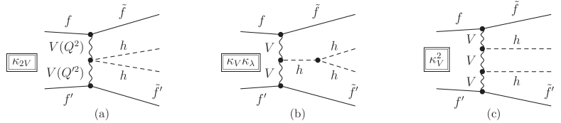
Before we turn to the relevance of the different couplings and their BSM reach, it is instructive to clarify the anticipated shape of the exclusion. WBF probes the incoming weak bosons at space-like momenta in the diagrams of Fig. 1. However, the analysis of scattering for physical momenta (the crossed process that enters WBF subdiagrams of Fig. 1) provides insight into gauge-symmetry cancellations that carry over into qualitative phenomenological outcomes via the effective approximation Dawson:1984gx ; Contino:2010mh . In the high energy limit , the polarised amplitudes scale as***This result can be straightforwardly obtained with FeynArts/FormCalc/LoopTools Hahn:1998yk ; Hahn:2000jm ; Hahn:2000kx , which we use throughout this work. Phase-space and polynomial suppression of the valence quark parton distribution functions significantly modify these naive expectations.
| (7) |
This shows that in the SM (as well as for direct Higgs mixing), we can expect a significant destructive interference to maintain unitarity at high energies. The scaling with energy in the WBF process is pdf-suppressed for massless partons (including in the effective approximation), however, large enough deviations from the SM correlation manifest themselves as an enhanced cross section so that limits can be set. Note that does not enter the amplitude with energy enhancement, and its constraints are therefore set by a priori perturbativity limits (see DiLuzio:2017tfn ; Arco:2020ucn ; Arco:2022lai for more model-specific considerations).
2.1 Hadron collider constraints on and
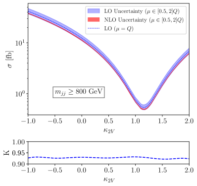
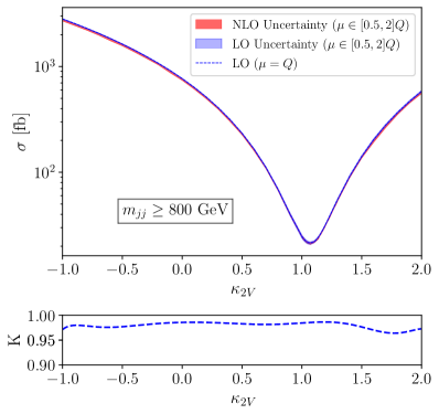
production follows production from the point of view of QCD. Therefore, the search region that is selected by the LHC experiments exploits the usual WBF paradigm Cahn:1983ip ; Rainwater:1998kj ; Zeppenfeld:2000td ; Figy:2003nv . Similar to the findings in single-Higgs and double-Higgs production via WBF Figy:2008zd ; Dreyer:2018qbw , the QCD corrections can be formidably captured through an adapted choice of the renormalisation and factorisation scales, due to the process’ ‘double-Deep Inelastic Scattering’ structure. In particular, in the measurement region selected by the LHC experiments then becomes extraordinarily stable: In Fig. 2 we show the WBF cross section component at next-to-leading order QCD in comparison to the leading order estimate, employing the central scale choice (cf. Fig. 1) for the signal region characterised by an invariant jet mass of .†††We obtain this through a modification of the publicly available Vbfnlo Monte Carlo programme Figy:2003nv ; Arnold:2008rz ; Baglio:2012np . Modifications have been cross-checked against MadGraph_aMC@NLO Alwall:2014hca . See also Frederix:2014hta for studies of rescalings of the Higgs self-coupling. This extends to the FCC-hh at a significantly increased cross-section, Fig. 2. The cross-section is well-approximated by the LO choice, and the NLO corrections are modest at the LHC, decreasing in relevance at the FCC-hh, running at 100 TeV FCC:2018vvp . The key limitation of setting constraints on is then statistics and background systematics.
The ATLAS Collaboration has previously published search results for nonresonant production using of early Run 2 data ATLAS:2018rnh , as well as a dedicated search for VBF production in of data collected between 2016 and 2018 ATLAS:2020jgy . The latest analysis ATLAS:2023qzf builds upon these earlier results by incorporating the 2016–2018 data for both production channels and taking advantage of improvements in jet reconstruction and -tagging techniques. Notably, the analysis employs an entirely data-driven technique for background estimation, utilising an artificial neural network to perform kinematic reweighting of data to model the background in the region of interest, and it currently restricts to
| (8) |
The CMS Collaboration has also published results of a search for nonresonant with its full Run 2 dataset CMS:2022cpr , which restricts the allowed interval for to , at confidence level (CL). Furthermore, a more recent CMS publication CMS:2022nmn that exploits topologies arising from highly energetic Higgs boson decays into , restricts the allowed interval for to
| (9) |
ATLAS and CMS have conducted investigations into non-resonant in the ATLAS:2022xzm ; CMS:2017hea ; CMS:2017yfv ; CMS:2022hgz ; ATLAS:2015sxd and ATLAS:2021ifb ; CMS:2020tkr ; ATLAS:2015sxd decay channels as well. In our analysis, we look at final state topologies for the highest di-Higgs branching ratios, i.e.,
| (10a) | |||
| and, | |||
| (10b) | |||
We generate events for each process scanning over the space of and , keeping fixed, and perform a fit to obtain the limits on the corresponding couplings.
Event generation and selection
To investigate WBF processes, we use MadGraph_aMC@NLO Alwall:2014hca with leading order precision at to generate our events and apply stringent cuts at the generator level on the WBF jet pair’s invariant mass ( GeV). Additionally, we set the pseudorapidity of the -jets to be to ensure that the -jets produced from the Higgs pair are centrally located. We modify the MadGraph source code to include the modifiers for event generation. Subsequently, we shower the events with Pythia 8.3 Bierlich:2022pfr and use MadAnalysis Conte:2012fm that interfaces FastJet Cacciari:2011ma ; Cacciari:2005hq , to reconstruct the final state particles with a -tagging efficiency.
Firstly, we define forward and central jets with the following selection criteria:
-
1.
Forward jets: and .
-
2.
Central jets: and .
To select events in the channel, we utilise the methodology described in ATLAS:2023qzf . Initially, we identify the jet pair with the highest invariant mass as the WBF jets and impose the forward-jet criteria on them. Next, we require at least 4 centrally located jets, all of which must be -tagged. We also apply an additional pseudorapidity separation cut of and an invariant mass cut of on the WBF-jets. To isolate the WBF region, we further demand that the transverse component of the momentum vector sum of the two WBF jets and the four jets forming the Higgs boson candidates be less than . The Higgs pair is constructed from the 4 -jets and a minimum invariant mass of is required.
For the channel, the WBF jet pair is chosen in the same manner as before, and we apply the same cuts on them. However, only two centrally located -tagged jets are required in this case. The -leptons can decay either hadronically or leptonically, with the latter being selected using the criteria outlined in the latest ATLAS analysis ATLAS:2022xzm , with a minimum of and limited to . The light jets arising from the hadronic decay of the -leptons are selected with a minimum of and . Additionally, the leptonic decay of the ’s results in missing energy. The di-Higgs invariant mass is then constructed using the two -jets and the -decay products, with a minimum invariant mass requirement of .
Sensitivity and projections
We use the distribution of the reconstructed kinematic observable to obtain the current and projected limits on the respective couplings. The statistic for our analysis is computed as
| (11a) | |||
| where represents the combined number of events in the th bin of from both decay channel, considering their respective cross-sections and efficiency, at a given luminosity for a particular value of and , and corresponds to the expected number of events solely from the SM for and . The covariance matrix is the sum-in-quadrature of two terms: 1) the statistical uncertainties computed from the root of bin entries, i.e., the Poisson uncertainty associated with each bin, , and 2) fully correlated relative fractional uncertainties (), i.e., | |||
| (11b) | |||
To fix , we set and scan over such that we reproduce a 95% CL limit of at at the LHC, comparable to the limits set by ATLAS ATLAS:2023qzf and CMS CMS:2022nmn .
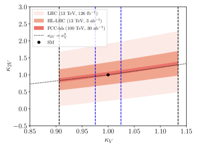
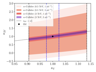
Once our methodology was validated through a comparison of our constraints with the predictions of ATLAS (Eq. 8) and CMS (Eq. 9), we proceed to explore the parameter space of and and obtain constraints at the CL. Our results are presented in Fig. 3, where we show the confidence bands for the LHC with an integrated luminosity of , the constraints for the High-Luminosity (HL-LHC) frontier with an integrated luminosity of , as well as the projected constraints for the Future Circular Collider (FCC-hh) with and an integrated luminosity of , assuming the same as for the LHC case. It should be added that using the calibrated to ATLAS:2023qzf ; CMS:2022nmn is a conservative extrapolation for the FCC-hh. A limiting factor in this environment is the reduction of QCD multi-jet contributions as central jet vetoes are not available to suppress these efficiently. This can lead to a considerable variation of the expected sensitivity Dolan:2013rja ; Dolan:2015zja ; Bishara:2016kjn , in particular when considering the rejection of the irreducible gluon fusion component.
2.2 Lepton collider constraints on and
The di-Higgs sector exploration at upcoming lepton colliders has garnered significant attention due to their exceptional sensitivity range, which is attributed to significantly lower background interference compared to hadron colliders. The works of Chacko:2017xpd ; DiVita:2017vrr ; Li:2017daq ; Abramowicz:2016zbo (see also Refs. Domenech:2022uud ; Gonzalez-Lopez:2020lpd ) have been instrumental in investigating the di-Higgs sector and obtaining exclusion limits on and . Building on this success, we extend the scope of this exploration by attempting to obtain limits on and for -colliders, adopting a methodology similar to that presented in Sec. 2.1. In this scenario, the di-Higgs decay into four -quarks is very attractive since the background is orders of magnitude smaller, making it the primary focus of our analysis. The process we want to look at is, therefore,
| (12) |
The dominant contributions to the production cross-section come from the WBF process and Higgs-strahlung. We generate our events with MadGraph for two benchmark collider beam energies of and . To select our WBF signal region, we closely follow the analysis in Chacko:2017xpd . We firstly impose a strict missing energy cut greater than . Our study further requires four centrally located -tagged jets, with and . In order to reconstruct the Higgses individually from the ’s, we determine the labelling of the four -jets, , that minimises the quantity , where represents the invariant mass formed by jets and . We infer that , come from one of the Higgs decay, and , are the decay products of the other. We then demand that the corresponding jets reconstruct the two Higgs bosons within the on-shell window ().
With the selected signal events, we construct a as described in Sec. 2.1, again, scanning over and . The constraints for both our benchmark points are presented in Fig. 3, at integrated luminosities of and . Our analysis reproduces the CLIC projection Roloff:2019crr ,
| (13) |
However, the potential to exploit beam polarisations in Roloff:2019crr (which we do not, here in our comparison) indicates that our sensitivity estimates are conservative.
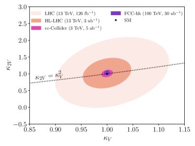
In the following sections, we will treat the single Higgs constraints independently from the constraints for presentation purposes (in our discussion below, these limits correspond to qualitatively different phenomenological parameters). Of course, the individual rectangular regions indicated in Fig. 3 are simultaneously constrained by these (correlated) data sets. To gauge how the rectangular regions map onto the elliptical constraints in a combination of this information for the most sensitive environments, we show a combination of single Higgs and weak boson fusion production in Fig. 4. This demonstrates that in particular at the very sensitive future collider environments that enable tight constraints on , this parameter will remain less constrained compared to .
Remarks on
Weak boson fusion processes at hadron colliders play a less relevant role in constraining Higgs self-interactions, predominantly the trilinear Higgs coupling, as Higgs pair production from gluon fusion is more abundant. Representative extrapolations to the HL-LHC phase Cepeda:2019klc indicate that this coupling could be constrained at 50% around its SM expectation. The environment of an FCC-hh at 100 TeV will increase the sensitivity to 3-5% Contino:2016spe .
Higgs self-coupling measurements at lepton colliders are dominated by -boson associated Higgs pair production for low centre-of-mass energies and WBF at large energies, e.g., at CLIC. The latter, maximising the WBF potential, has a projected sensitivity of about with some level of degeneracy between and Roloff:2019crr . As for hadron colliders the constraint on is stronger compared to which highlights the need for constraining at hadron colliders such as the LHC. The sensitivity at CLIC compares to an estimated ILC sensitivity (in the 250 GeV+500 GeV combined phase) of ILC:2019gyn .
The main focus of our work is a discussion of in WBF as this channel is primarily sensitive to these parameters due to Eq. 7. We will include, however, details on and its relevance in comparison to in the discussion of the next Sec. 3. is known to be relatively efficiently constrainable in gluon fusion Higgs pair production through sensitivity in the threshold region, whose inclusive cross section Baur:2002rb ; Dolan:2012rv is an order of magnitude larger than WBF. Our discussion of should therefore be understood as a potential additional constraint when considering measurements as performed by the experiments.
3 , and in BSM models
In this Section, we consider how different BSM models populate the space of , , and . We pay particular attention to those models that predict order-of-magnitude larger deviations in either or relative to ; in such cases future measurements of either or are likely to provide significant discriminating power. As discussed recently in Alonso:2021rac , and as we elucidate below, a large deviation in relative to will require non-decoupling TeV scale new physics.
3.1 Extended scalar sectors, tree level
Consider a generic extended scalar sector, built out of a set of electroweak multiplets . Let have an irreducible representation (irrep) of dimension , and a hypercharge , with renormalisable lagrangian
| (14) |
We define the charged current part of the covariant derivative to be
| (15) |
where the components of the generators in the irrep of dimension are given by
| (16) |
with the indices running between (labelling the component with maximum third component of isospin, ) and (labelling the component with minimum ).
The -th component is electrically neutral, and after electroweak symmetry breaking can be decomposed into vevs, and , and vev-free fields and
| (17) |
These are separated into real () and imaginary () parts. The imaginary components are absent from real irreps, as well as, without loss of generality, from one complex irrep due to our freedom to gauge it away. Assuming the scalar sector contains a hypercharge- doublet, we gauge away its imaginary component.
Substituting Eqs. 15 and 17 into Eq. 14 we see that in the broken phase the charged current interactions of the neutral Higgses are governed by
| (18) |
where index the neutral Higgses, and repeated indices are summed over, and the matrix is diagonal with entries
| (19) |
are the dimension and hypercharge of the multiplet from which the th component came: real and imaginary components of the same multiplet have the same entry. is normalised to be the identity matrix in an -Higgs doublet model.
The 125 GeV Higgs, , is defined as a unit direction in the space of neutral Higgs components:
| (20) |
We substitute the above into Eq. 18 and compare with Eq. 6. Identifying the total vev as
| (21) |
we obtain the coupling modifiers
| (22) |
Note that we have assumed the electroweak multiplets form complete custodial irreps, so that and .
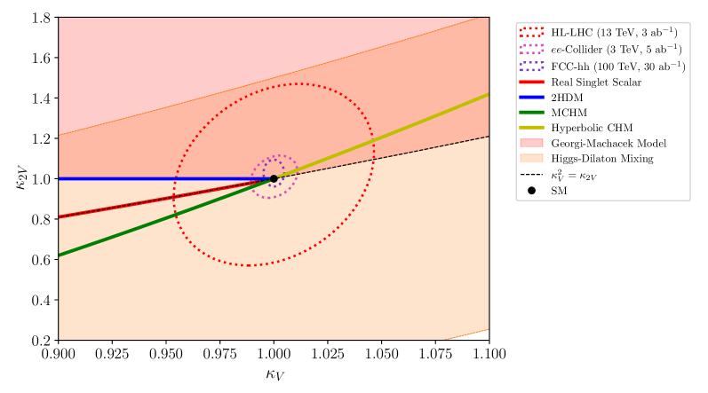
and are therefore correlated in particular extended scalar sectors, i.e. for particular . We give the examples of the singlet, second Higgs doublet, and Georgi-Machacek model in Table 2 and App. A. In Fig. 7, we show the lines and regions that these models can populate in the - plane. Notably, for any tree-level model
| (23) |
which follows from the Cauchy-Schwartz inequality when is a positive definite matrix. It is only zero in the alignment limit, when , or in the case of mixing with singlets, when is only positive semidefinite.
Thus, to obtain a large deviation in but not in an extended scalar sector, we require electroweak triplets or higher representations, and a departure from the alignment limit (i.e., a departure from the parabola ), see also Gunion:1989ci . This in turn implies significant mixing of components of the Higgs doublet with other states that cannot be made arbitrarily heavy. This is likely to cause some tension with direct searches. For instance, a significant triplet component to electroweak symmetry breaking introduces resonant tell-tale same-sign WBF production Englert:2013wga which drives constraints on the triplet nature of the observed Higgs boson CMS:2021wlt (see also Ismail:2020zoz ). Finally, we remark here that, in the decoupling limit, both and approach , and in principle do so from different directions in the - plane, depending on the model — compare, for instance, the singlet and 2HDM trajectories in Fig. 7. However, in the decoupling limit, the deviations from the Standard Model in due to are comparable to the short-distance contributions from heavy Higgs exchange. These latter exchange contributions are calculated for the singlet and 2HDM model in Egana-Ugrinovic:2015vgy , where this effect is discussed in detail. The effect of both and the short distance heavy Higgs exchange can be combined into a , which satisfies
| (24) |
in the decoupling limit. This corresponds to the pattern predicted by the SMEFT at dimension 6 (see, e.g., Alonso:2021rac ).
Turning now to , this is generally a free parameter for renormalisable potentials containing cubic interactions among the electroweak irreps. However, if the cubic interactions are absent (as often happens accidentally due to the charges of the multiplets, or is imposed by certain symmetries), we can begin to understand the range of close to the alignment limit. The potential among the neutral components before electroweak symmetry breaking will have the generic form
| (25) |
where the tensors and are necessarily symmetric in their indices, and corresponds to the electroweak symmetry preserving vacuum. After electroweak symmetry breaking, substituting leads to
| (26) |
where we’ve used the vev condition
| (27) |
From comparison with Eq. 6, takes the form
| (28) |
Close to the alignment limit, Eq. 28 can be expressed in terms of mass parameters and the degree of alignment. We work, without loss of generality, in the mass basis where the mass matrix of Eq. 26 satisfies
| (29) |
where label heavy Higgs directions, each with mass . In this basis, satisfies
| (30) |
for some small parameters describing the amount of the vev in the heavy Higgs directions when close to the alignment limit. Summation is implied over repeated indices.
In the decoupling limit, where are large, the model is necessarily aligned and are correspondingly small. The quartic couplings of the model are limited in size by perturbative unitarity, and so from Eq. 29 approaches . In this case
| (32) |
and the deviation in enjoys a parametric enhancement of relative to the deviations in and which are both . We note that this enhancement does not necessarily happen in the case of alignment without decoupling.
3.2 Extended scalar sectors, loop level
We turn to the case of an arbitrary electroweak scalar multiplet, , with a symmetry that prevents it from acquiring a vev, and a cross quartic interaction with the SM Higgs doublet :
| (33) |
If the scalar is sufficiently heavy, , its leading order effects are at one-loop level. When augmented with a small amount of splitting to allow charged particles to decay, Eq. 33 presents a minimal class of models that includes multiple viable candidates for BSM particles of mass Banta:2021dek . If the cross quartic is large, such that , sizeable effects in the electroweak phase transition are expected Banta:2022rwg .
In the simplest case of a symmetric singlet, and Eq. 33 reads
| (34) |
In this scenario the subamplitudes (as any amplitude) can be renormalised. We adopt the on-shell scheme as described in Ref. Ross:1973fp , which is the common scheme used for electroweak corrections (we are treating tadpoles as parameters as in Ref. Denner:2018opp ).‡‡‡Specifically, we choose as input parameters for the electroweak sector. The Weinberg angle is then a derived quantity Sirlin:1980nh . The effects of the singlet, to order , can be accounted for by substituting the following finite expressions into Fig. 1
| (35) |
Here , are the Passarino-Veltman Passarino:1978jh two-point function and its derivative, respectively, and is the 3-point function. becomes an -dependent form factor; this momentum dependence is particularly useful for light scalar masses which do not admit a reliable EFT description and can modify the phenomenology at threshold.
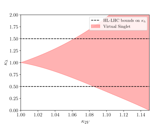
Note that, for the loop-level singlet, the correction to and is purely through the wavefunction renormalisation of the Higgs, and therefore follows a characteristic pattern, the corrections to both scaling as . , on the other hand, receives a contribution from a 1PI singlet loop. When is large, this generically means the sensitivity to this model at HL-LHC is greater than that of , as illustrated in Fig. 5.
In principle, a with non-trivial electroweak charges can contribute 1PI corrections to and vertices; in practice, however, these states’ corrections to the parameters are parametrically similar to the singlet case. To see this, take to be a second (inert) Higgs doublet as a representative example, and work to order , assuming the extra states are sufficiently heavy for their effects in to be well approximated by constant s. Performing the same calculation as before in the on-shell scheme we obtain, for the off-shell SM-like 1 particle irreducible vertex functions ,
| (36) | ||||
We highlight the fact that these are no longer related to physical quantities by introducing the bar. The physical couplings in the amplitudes are the product of both these corrections to the s, and the corrections to the electroweak couplings due to the non-trivial gauge quantum numbers of the new fields. In particular, for non-vanishing hypercharge, the new states are additional sources of custodial isospin violation as directly visible above. The gaugeless part of the corrections mirrors those of the singlet Eq. 35. In particular, the corrections to and come exclusively from wavefunction normalisation of the Higgs boson.§§§Parametrically comparable 1PI contributions to and arise from dimension-six operators . In cases where couplings are forbidden by gauge-invariance, Eq. 1, the dimension-6 contributions are conventionally included to the definition as is the case for , see e.g. Djouadi:2005gi ; Carmi:2012in .
The above results clearly show that additional gauge interactions can sculpt the parameter regions, however in a phenomenologically highly suppressed way compared to new additional inter-scalar interactions. Focussing on the gauge-independent part in practical analyses, the contributions all scale with the number of real degrees of freedom, . This gives approximate values for an arbitrary irrep of
| (37) | ||||
where we have assumed to drop the piece in , and focused on the HL-LHC measurement region . The full momentum dependence for any such irrep can be restored from Eq. 35 by multiplying by the dimension .
3.3 From compositeness to dilaton mixing
The values of a composite Higgs model depend on the details of the symmetry breaking. In the minimal composite Higgs model (MCHM), the components of the Higgs doublet chart the coset Contino:2003ve ; Agashe:2004rs ; Contino:2006qr , whose relevant dynamics are readily constructed through the linear sigma model, see Alonso:2016btr . The five components have kinetic terms
| (38) |
where the first four components have SM-like gauge couplings to the and . The components are restricted to the surface
| (39) |
which, in unitary gauge, can be parametrised by
| (40) |
where is understood to be the Higgs coordinate shifted such that in the absence of electroweak symmetry breaking. Substitution of Eq. 40 into Eq. 38 yields the unitary gauge lagrangian
| (41) |
and expanding about the vacuum then gives
| (42) |
in terms of . While this pattern will change for different cosets, it was shown in Alonso:2016oah that for all custodial-symmetry-preserving cosets arising from the breaking of a compact group, it is guaranteed that
| (43) |
By contrast, this can be violated for non-compact groups. A non-compact coset can be constructed via the linear sigma model lagrangian Alonso:2016btr
| (44) |
restricted to the surface
| (45) |
which is parametrised in unitary gauge by
| (46) |
(Note that trigonometric functions in Eq. 40 become hyperbolic ones in Eq. 46, similar in spirit to the compactification of the Lorentz group.) This yields
| (47) |
for the hyperbolic composite Higgs model.
In composite Higgs theories, the Higgs potential can be written schematically in MCHM5 (and MCHM5-like theories such as Ref. Ferretti:2014qta , where the 5 refers to the spurionic irrep of the top quark) as
| (48) |
where is a constant, see also Contino:2010rs . The coefficients are related to two and four-point functions of the underlying strongly interacting theory Golterman:2015zwa ; DelDebbio:2017ini responsible for partial compositeness, and they can be replaced as a function of and the Higgs mass. These coefficients can in principle be inferred from lattice computations (for recent progress see Ayyar:2018glg ; DelDebbio:2022qgu ) to uncover realistic UV completions. The Higgs trilinear coupling modifier is then given by
| (49) |
The expression for the hyperbolic composite Higgs model is again obtained from the replacement Alonso:2016btr .
We note that the above expressions satisfy
| (50) |
Therefore Fig. 1(a) reproduces the behaviour of Fig. 1(b) at leading order in the MCHM5 scenario. This is due to the symmetry breaking potential being of the same functional form as the interaction of the Goldstone bosons.¶¶¶ In MCHM4 the potential reads leading to , see also Grober:2010yv . In this scenario, which suffers from tension with electroweak precision constraints, we also have .
Ultimately, the value of depends on the (spurionic) representations of the explicit symmetry breaking in the model. Larger representations, leading to higher order Gegenbauer polynomials of in the potential, can break the above correlation between and , and generally lead to a parametric enhancement in the deviations of from the Standard Model Durieux:2021riy .
3.3.1 Deforming the MCHM with a dilaton
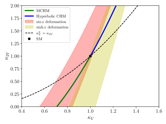
The MCHM, together with its hyperbolic counterpart, define a line in the - plane (shown in green and blue in Fig. 6) corresponding to the maximally symmetric coset spaces of constant positive or negative curvature alma9938889293902959 . Reference Alonso:2021rac considered deformations away from this line that can arise from deformations of the coset space. Here, we begin similarly, and argue that a viable model for these deformations comes from mixing of the composite Higgs with a TeV scale dilaton.
Practically, the coset space can be deformed by replacing the constant radius in Eqs. 39 and 45 with a mildly dependent function
| (51) |
for some . This promotes to a modulus that is common in higher dimensional theories of electroweak symmetry breaking.∥∥∥The motivation of the scalar metric from which this theory derives also follows the discussion presented in Bekenstein:1992pj . We have expanded to order , assuming the linear term is forbidden by symmetry, so a linear deformation will not change our findings qualitatively. We calculate the modifications , to linear order in , after performing a field redefinition to canonically normalise the kinetic terms. (This field redefinition necessarily introduces momentum-dependent self-interactions of the would-be Higgs boson, to which we return below.) Scanning over , we see from Fig. 6 that such manifolds deviate from the line of uniform curvature in the - plane.
The effective dependence of can be brought about through mixing with a dilaton direction, , which we analyse here using the approach of Bruggisser:2022ofg . measures the departure from conformal symmetry through its vacuum expectation value Goldberger:2007zk . In a UV completion where the composite Higgs components are mesonic states arising from a confining gauge group , if the dilaton is another mesonic state, if the dilaton is a glueball like state Bruggisser:2022ofg . Here is a free parameter, which we require to be in order to get sizeable mixing effects with the composite Higgs states.
Interaction terms with the composite Higgs can be constructed by multiplying operators by , where is the canonical mass dimension of the operator, in order to restore conformal symmetry. Thus
| (52) |
in terms of the composite Higgs model operators Eqs. 41 and 48. Expanding this lagrangian around the minimum and including effects of Higgs-dilaton mixing through the usual isometry
| (53) |
we obtain, from the couplings of the mass eigenstate ,
| (54) |
where , and we have taken the MCHM5 potential for from Eq. 48.
These couplings indeed cover, a priori, a wide area in the - plane. In particular, the area , which was not populated by the models considered in previous sections, can be reached if the Higgs is considered mostly as a pseudo-dilaton. This area partially overlaps with the geometric deformations shown in Fig. 6 (Eq. 51 can be thought of as approximating the leading order effects of dilaton mixing).
can also accommodate large deviations from in the case of significant Higgs-dilaton mixing. In addition, the dilaton has additional terms from explicit sources of conformal symmetry violation as described in Rattazzi:2000hs ; Goldberger:2007zk . This means that trilinear interactions will receive momentum-dependent interactions as a consequence of the -theorem Komargodski:2011vj leading to
| (55) |
where the ellipses denote higher order terms in the dilaton and (see Komargodski:2011vj ; Dolan:2012ac ). This leads to an additional momentum-dependent modifications of of
| (56) |
with denoting the invariant di-Higgs mass. Modifications vanish close to the threshold, but can lead to a large modification of the invariant di-Higgs mass spectrum for considerable mixing.
The examples discussed so far exhaust the phenomenological possibilities in the - plane, and therefore provide a theoretical avenue to interpret the results of associated analyses. Of course, constraints are also informed by single Higgs measurements and therefore there are significant constraints on these scenarios from a range of experimental findings. Similarly, both momentum-dependent and momentum-independent modifications to are best constrained in measurements of gluon fusion Higgs pair production, given the larger rate and the generic sensitivity of WBF to (multi-) gauge boson interactions.
3.4 Running of coupling modifiers
Going beyond tree level, the correlations of , , and become scale and scheme dependent. In the Higgs effective field theory, the leading-order operators that modify , , and (free, uncorrelated parameters in HEFT) not only run into each other, but also into higher derivative, next-to-leading-order operators that modify the measured s, as shown in Table 1. To encapsulate these effects, we define an effective from the coefficient of in the effective vertex for (as defined in Herrero:2022krh ; Anisha:2022ctm )
| (57) |
with all legs on shell. The wavefunction normalisation of the Higgs is
| (58) |
in terms of the operator coefficient defined in Table 1 Herrero:2022krh . We obtain that
| (59) |
Similarly, from the value of
| (60) |
with all legs on shell we define an effective coupling
| (61) |
These effective couplings serve the purpose of effectively field-redefining the redundant higher derivative operators generated by the running back into and respectively. We do not define an analogous on-shell , as this would be a complicated function of components of the effective vertex and components of diagrams containing, e.g., and vertices.
Using the results of Herrero:2021iqt ; Herrero:2022krh (see also Delgado:2013hxa ; Gavela:2014uta ; Asiain:2021lch ; Gomez-Ambrosio:2022why ; Gomez-Ambrosio:2022qsi ; Anisha:2022ctm ), the couplings run according to
| (62) |
is the multiplicative modifier of the vertex, and is set to one in the following. We have chosen to present the running of in terms of that of the combination , which controls the energy growth of the process.
The Standard Model is a fixed point of the running, as the RHSs of Eq. 62 vanish when .******Without defining to take account of the effect of the higher derivative operators, would appear to run even at the Standard Model point. Linearising the RGEs about this point by defining
| (63) |
we find
| (64) |
up to corrections. Note that, to expand the RHS of Eq. 62, we have assumed we are running from a point where all higher order coefficients are zero.
We note from Eq. 64 that , which is experimentally the least constrained of the three parameters, self-renormalises significantly stronger than the other two. Also, the negative coefficient for the self-renormalisation of means that a positive , as is the case for all renormalisable models, grows in the IR, away from the alignment limit.
| Model | Ref. | ||
| Singlet | §A.1 | ||
| 2HDM | §A.2 | ||
| Georgi-Machacek | §A.3 | ||
| Tree-level scalar | §3.1 | ||
| Loop-level scalar | §3.2 | ||
| (large ) | |||
| SMEFT | free | e.g. Grzadkowski:2010es ; Dedes:2017zog | |
| MCHM | §3.3 | ||
| MCHM + Dilaton | §3.3 | ||
| HEFT | free | free | e.g. Herrero:2021iqt |
4 Conclusions
Analyses employing Feynman diagrams as templates are established approaches in the experimental community CMS:2022nmn ; ATLAS:2023qzf in situations where data is expected to be limited, even at the high-luminosity phase of the LHC or stretches of future collider runs. What can be learned from them? To answer this question and provide an ab initio motivation for these analyses, we have performed such a templated analysis of future sensitivity in the WBF di-Higgs channel to the coupling modifiers , and we have scanned a range of BSM models to understand their pattern of effects in the same three coupling modifiers.
Fig. 7 shows projected future constraints on the - plane from the WBF di-Higgs process. This translates into approximate bounds on deviations in the single parameter of order for HL-LHC, and order for future colliders. These are to be contrasted with bounds on from single Higgs measurements that are approximately an order of magnitude smaller.
On the theoretical side, deviations in and are highly correlated in all models of heavy, decoupling new physics. This can be understood through their SMEFT parametrisation, where, due to the doublet nature of the Higgs field, at dimension 6. In the broader HEFT parametrisation, and are independent free parameters due to the custodial iso-singlet parameterisation of the Higgs boson. Any models of non-decoupling new physics where the deviation in is an order of magnitude larger than that in would highly motivate WBF di-Higgs production as an indirect probe of new physics.
To this end, we surveyed many BSM models in Sec. 3, and summarise their patterns of effects in and in Table 2. In sum, to achieve an enhancement in within an extended scalar sector requires tree-level mixing with triplets or higher electroweak representations. This cannot be done at loop level, where extra scalars give a characteristic pattern from wavefunction renormalisation of the Higgs. We note in passing, however, that we have identified a large class of scalar extensions of the SM for which a Feynman-templated analysis extends to one-loop BSM precision in the weak sector.
We find that all renormalisable extended scalar sectors satisfy , with this quantity growing in the IR due to running effects. As also controls the energy growth of longitudinal -Higgs scattering, it is possible that a sum rule type argument could yield further insight into this sign. is achievable, however, in non-renormalisable models of the scalar sector. The archetype of such a model — the minimal composite Higgs model — follows the SMEFT pattern, as it smoothly decouples in the limit. However, it is possible to obtain a large (and negative) deviation in in composite Higgs models which contain a TeV scale dilaton.
Our investigation therefore shows that the Feynman diagram-based explorations of the WBF channel add important value to the phenomenology programme, at the LHC and beyond. can significantly depart from the SM correlation with , and the loose constraints on probe parameter regions of BSM scenario that are not accessible by a precision study of alone. This is assisted by considerable stability of the WBF cross sections from the point of view of QCD. However, measurable deviations in come at the price of significant tree-level mixing at the TeV scale in either perturbative (extended scalar sectors containing higher electroweak irreps) or non-perturbative (composite Higgs with dilaton) scenarios. The size of tree-level mixing highlights the relevance of direct searches. To compare the power of direct searches, let us briefly consider the prospects at the LHC for the Georgi-Machacek and composite Higgs with dilaton models.
For the Georgi-Machacek model, tell-tale and experimentally clean signatures arise from the doubly charged, gauge-philic Higgs boson, whose interactions are sensitive to the triplets’ contribution to the electroweak vacuum. Recent constraints ATLAS:2023dbw limit for masses below 1 TeV. A luminosity-based extrapolation should further decrease this by a factor of two for HL-LHC. Using the expressions in Table 2 with and gives a possible range of from current (future) LHC resonance searches, which is comparable to the constraints from di-Higgs measurements.
For the composite Higgs models, including those which mix with a dilaton, one expects other composite resonances to appear at a scale below , assuming . Arguably, the most model independent predictions of the composite Higgs do not yet meet this threshold: the pair production of top partners is currently bounded up to masses of around ATLAS:2022hnn , and the electroweak production and decay of a heavy vector triplet — analogous to in QCD — is currently bounded up to masses of around ATLAS:2020fry . This latter bound is limited by the collision energy of the LHC, and is unlikely to improve significantly with increased luminosity. Therefore, using the expressions in Table 2 with and gives a possible range of . We note that, if the dilaton has (model dependently) a coupling to gluons, a direct search for the dilaton in could rule out a significant amount of this parameter space Bruggisser:2022ofg .
Finally, although plays a subdominant phenomenological role in WBF production in a hadron collider, in many of the scenarios that we have considered in this work, more susceptible to deviations from the SM compared to . Examples include tree-level extended scalar sectors in the alignment with decoupling limit, loop-level scalars with sizeable cross-quartic interactions with the Higgs doublet, and composite Higgs models containing explicit symmetry breaking terms in higher spurionic irreps. As can be dominantly extracted from analyses, correlations observed in the WBF mode will add further exclusion potential.
Acknowledgements.
We thank Aidan Robson and Panagiotis Stylianou for helpful conversations. C.E. is supported by the STFC under grant ST/T000945/1, the Leverhulme Trust under grant RPG-2021-031. C.E. and D.S. acknowledge support from the Institute for Particle Physics Phenomenology Associateship Scheme. W.N. is funded by a University of Glasgow College of Science and Engineering Scholarship.Appendix A and in specific scalar models
Here we give the and values at tree level in specific extended scalar sectors, using the master formulae Eqs. 19 and 22.
A.1 Higgs + singlet
In unitary gauge, there is one neutral component of the Higgs doublet and one from the singlet, with matrix
| (65) |
Writing and , we have
| (66) | ||||
| (67) |
as expected.
A.2 2HDM
In unitary gauge there are two scalar neutral components, which both generically contain vevs and mix among each other, and a pseudoscalar neutral component which, when custodial symmetry is imposed, obtains no vev and does not mix with the other neutral components Gunion:1989ci (see the recent Arco:2023sac for the 2HDMs relation to HEFT). The matrix is the identity matrix,
| (68) |
Writing
| (69) | ||||
| (70) |
where the third entry is associated with the pseudoscalar component, we obtain
| (71) | ||||
| (72) |
A.3 Georgi-Machacek
Ordering the neutral components respectively as that of the Higgs doublet, the two components of the complex triplet and the one component of the real triplet, the matrix is
| (73) |
Custodial symmetry implies that among the triplet components, and also that the mass matrix is invariant under permutations among the 2, 3 and 4 indices, meaning in the light Higgs eigenvector Hartling:2014zca . Thus we can write
| (74) | ||||
| (75) |
which implies that
| (76) | ||||
| (77) |
We have also reproduced this result using the mass matrices of Hartling:2014zca , see also Alonso:2021rac .
References
- (1) LHC Higgs Cross Section Working Group collaboration, S. Dittmaier et al., Handbook of LHC Higgs Cross Sections: 1. Inclusive Observables, 1101.0593.
- (2) ATLAS collaboration, G. Aad et al., Search for nonresonant pair production of Higgs bosons in the final state in collisions at TeV with the ATLAS detector, 2301.03212.
- (3) ATLAS collaboration, G. Aad et al., Searches for Higgs boson pair production in the channels with the ATLAS detector, Phys. Rev. D 92 (2015) 092004, [1509.04670].
- (4) CMS collaboration, A. M. Sirunyan et al., Search for Higgs boson pair production in events with two bottom quarks and two tau leptons in proton–proton collisions at =13TeV, Phys. Lett. B 778 (2018) 101–127, [1707.02909].
- (5) CMS collaboration, A. M. Sirunyan et al., Search for Higgs boson pair production in the final state in proton-proton collisions at = 8 TeV, Phys. Rev. D 96 (2017) 072004, [1707.00350].
- (6) CMS collaboration, A. M. Sirunyan et al., Search for nonresonant Higgs boson pair production in final states with two bottom quarks and two photons in proton-proton collisions at = 13 TeV, JHEP 03 (2021) 257, [2011.12373].
- (7) ATLAS collaboration, G. Aad et al., Search for Higgs boson pair production in the two bottom quarks plus two photons final state in collisions at = 13 TeV with the ATLAS detector, Phys. Rev. D 106 (2022) 052001, [2112.11876].
- (8) CMS collaboration, A. M. Sirunyan et al., Search for nonresonant Higgs boson pair production in final state with two bottom quarks and two tau leptons in proton-proton collisions at = 13 TeV, 2206.09401.
- (9) ATLAS collaboration, G. Aad et al., Search for resonant and non-resonant Higgs boson pair production in the decay channel using 13 TeV collision data from the ATLAS detector, 2209.10910.
- (10) B. Grzadkowski, M. Iskrzynski, M. Misiak and J. Rosiek, Dimension-Six Terms in the Standard Model Lagrangian, JHEP 10 (2010) 085, [1008.4884].
- (11) M. McCullough, An Indirect Model-Dependent Probe of the Higgs Self-Coupling, Phys. Rev. D 90 (2014) 015001, [1312.3322].
- (12) G. Degrassi, P. P. Giardino, F. Maltoni and D. Pagani, Probing the Higgs self coupling via single Higgs production at the LHC, JHEP 12 (2016) 080, [1607.04251].
- (13) M. Gorbahn and U. Haisch, Indirect probes of the trilinear Higgs coupling: and , JHEP 10 (2016) 094, [1607.03773].
- (14) G. D. Kribs, A. Maier, H. Rzehak, M. Spannowsky and P. Waite, Electroweak oblique parameters as a probe of the trilinear Higgs boson self-interaction, Phys. Rev. D 95 (2017) 093004, [1702.07678].
- (15) Anisha, O. Atkinson, A. Bhardwaj, C. Englert and P. Stylianou, Quartic Gauge-Higgs couplings: constraints and future directions, JHEP 10 (2022) 172, [2208.09334].
- (16) K. Agashe, R. Contino and A. Pomarol, The Minimal composite Higgs model, Nucl. Phys. B 719 (2005) 165–187, [hep-ph/0412089].
- (17) R. Contino, L. Da Rold and A. Pomarol, Light custodians in natural composite Higgs models, Phys. Rev. D 75 (2007) 055014, [hep-ph/0612048].
- (18) S. R. Coleman, J. Wess and B. Zumino, Structure of phenomenological Lagrangians. 1., Phys. Rev. 177 (1969) 2239–2247.
- (19) C. G. Callan, Jr., S. R. Coleman, J. Wess and B. Zumino, Structure of phenomenological Lagrangians. 2., Phys. Rev. 177 (1969) 2247–2250.
- (20) T. Binoth and J. J. van der Bij, Influence of strongly coupled, hidden scalars on Higgs signals, Z. Phys. C 75 (1997) 17–25, [hep-ph/9608245].
- (21) B. Patt and F. Wilczek, Higgs-field portal into hidden sectors, hep-ph/0605188.
- (22) R. M. Schabinger and J. D. Wells, A Minimal spontaneously broken hidden sector and its impact on Higgs boson physics at the large hadron collider, Phys. Rev. D 72 (2005) 093007, [hep-ph/0509209].
- (23) C. Englert, T. Plehn, D. Zerwas and P. M. Zerwas, Exploring the Higgs portal, Phys. Lett. B 703 (2011) 298–305, [1106.3097].
- (24) R. Alonso, E. E. Jenkins and A. V. Manohar, A Geometric Formulation of Higgs Effective Field Theory: Measuring the Curvature of Scalar Field Space, Phys. Lett. B 754 (2016) 335–342, [1511.00724].
- (25) S. Dawson, The Effective W Approximation, Nucl. Phys. B 249 (1985) 42–60.
- (26) R. Contino, C. Grojean, M. Moretti, F. Piccinini and R. Rattazzi, Strong Double Higgs Production at the LHC, JHEP 05 (2010) 089, [1002.1011].
- (27) T. Hahn and M. Perez-Victoria, Automatized one loop calculations in four-dimensions and D-dimensions, Comput. Phys. Commun. 118 (1999) 153–165, [hep-ph/9807565].
- (28) T. Hahn, Automatic loop calculations with FeynArts, FormCalc, and LoopTools, Nucl. Phys. B Proc. Suppl. 89 (2000) 231–236, [hep-ph/0005029].
- (29) T. Hahn, Generating Feynman diagrams and amplitudes with FeynArts 3, Comput. Phys. Commun. 140 (2001) 418–431, [hep-ph/0012260].
- (30) L. Di Luzio, R. Gröber and M. Spannowsky, Maxi-sizing the trilinear Higgs self-coupling: how large could it be?, Eur. Phys. J. C 77 (2017) 788, [1704.02311].
- (31) F. Arco, S. Heinemeyer and M. J. Herrero, Exploring sizable triple Higgs couplings in the 2HDM, Eur. Phys. J. C 80 (2020) 884, [2005.10576].
- (32) F. Arco, S. Heinemeyer, M. Mühlleitner and K. Radchenko, Sensitivity to Triple Higgs Couplings via Di-Higgs Production in the 2HDM at the (HL-)LHC, 2212.11242.
- (33) R. N. Cahn and S. Dawson, Production of Very Massive Higgs Bosons, Phys. Lett. B 136 (1984) 196.
- (34) D. L. Rainwater, D. Zeppenfeld and K. Hagiwara, Searching for in weak boson fusion at the CERN LHC, Phys. Rev. D 59 (1998) 014037, [hep-ph/9808468].
- (35) D. Zeppenfeld, R. Kinnunen, A. Nikitenko and E. Richter-Was, Measuring Higgs boson couplings at the CERN LHC, Phys. Rev. D 62 (2000) 013009, [hep-ph/0002036].
- (36) T. Figy, C. Oleari and D. Zeppenfeld, Next-to-leading order jet distributions for Higgs boson production via weak boson fusion, Phys. Rev. D 68 (2003) 073005, [hep-ph/0306109].
- (37) T. Figy, Next-to-leading order QCD corrections to light Higgs Pair production via vector boson fusion, Mod. Phys. Lett. A 23 (2008) 1961–1973, [0806.2200].
- (38) F. A. Dreyer and A. Karlberg, Vector-Boson Fusion Higgs Pair Production at N3LO, Phys. Rev. D 98 (2018) 114016, [1811.07906].
- (39) K. Arnold et al., VBFNLO: A Parton level Monte Carlo for processes with electroweak bosons, Comput. Phys. Commun. 180 (2009) 1661–1670, [0811.4559].
- (40) J. Baglio, A. Djouadi, R. Gröber, M. M. Mühlleitner, J. Quevillon and M. Spira, The measurement of the Higgs self-coupling at the LHC: theoretical status, JHEP 04 (2013) 151, [1212.5581].
- (41) J. Alwall, R. Frederix, S. Frixione, V. Hirschi, F. Maltoni, O. Mattelaer et al., The automated computation of tree-level and next-to-leading order differential cross sections, and their matching to parton shower simulations, JHEP 07 (2014) 079, [1405.0301].
- (42) R. Frederix, S. Frixione, V. Hirschi, F. Maltoni, O. Mattelaer, P. Torrielli et al., Higgs pair production at the LHC with NLO and parton-shower effects, Phys. Lett. B 732 (2014) 142–149, [1401.7340].
- (43) FCC collaboration, A. Abada et al., FCC-hh: The Hadron Collider: Future Circular Collider Conceptual Design Report Volume 3, Eur. Phys. J. ST 228 (2019) 755–1107.
- (44) ATLAS collaboration, M. Aaboud et al., Search for pair production of Higgs bosons in the final state using proton-proton collisions at TeV with the ATLAS detector, JHEP 01 (2019) 030, [1804.06174].
- (45) ATLAS collaboration, G. Aad et al., Search for the process via vector-boson fusion production using proton-proton collisions at TeV with the ATLAS detector, JHEP 07 (2020) 108, [2001.05178].
- (46) CMS collaboration, A. Tumasyan et al., Search for Higgs Boson Pair Production in the Four b Quark Final State in Proton-Proton Collisions at = 13 TeV, Phys. Rev. Lett. 129 (2022) 081802, [2202.09617].
- (47) CMS collaboration, A. M. Sirunyan et al., Search for nonresonant pair production of highly energetic Higgs bosons decaying to bottom quarks, 2205.06667.
- (48) C. Bierlich et al., A comprehensive guide to the physics and usage of PYTHIA 8.3, 2203.11601.
- (49) E. Conte, B. Fuks and G. Serret, MadAnalysis 5, A User-Friendly Framework for Collider Phenomenology, Comput. Phys. Commun. 184 (2013) 222–256, [1206.1599].
- (50) M. Cacciari, G. P. Salam and G. Soyez, FastJet User Manual, Eur. Phys. J. C 72 (2012) 1896, [1111.6097].
- (51) M. Cacciari and G. P. Salam, Dispelling the myth for the jet-finder, Phys. Lett. B 641 (2006) 57–61, [hep-ph/0512210].
- (52) M. J. Dolan, C. Englert, N. Greiner and M. Spannowsky, Further on up the road: production at the LHC, Phys. Rev. Lett. 112 (2014) 101802, [1310.1084].
- (53) M. J. Dolan, C. Englert, N. Greiner, K. Nordstrom and M. Spannowsky, production at the LHC, Eur. Phys. J. C 75 (2015) 387, [1506.08008].
- (54) F. Bishara, R. Contino and J. Rojo, Higgs pair production in vector-boson fusion at the LHC and beyond, Eur. Phys. J. C 77 (2017) 481, [1611.03860].
- (55) ATLAS collaboration, G. Aad et al., A detailed map of Higgs boson interactions by the ATLAS experiment ten years after the discovery, Nature 607 (2022) 52–59, [2207.00092].
- (56) Z. Chacko, C. Kilic, S. Najjari and C. B. Verhaaren, Testing the Scalar Sector of the Twin Higgs Model at Colliders, Phys. Rev. D 97 (2018) 055031, [1711.05300].
- (57) S. Di Vita, G. Durieux, C. Grojean, J. Gu, Z. Liu, G. Panico et al., A global view on the Higgs self-coupling at lepton colliders, JHEP 02 (2018) 178, [1711.03978].
- (58) B. Li, Z.-L. Han and Y. Liao, Higgs production at future e+e- colliders in the Georgi-Machacek model, JHEP 02 (2018) 007, [1710.00184].
- (59) H. Abramowicz et al., Higgs physics at the CLIC electron–positron linear collider, Eur. Phys. J. C 77 (2017) 475, [1608.07538].
- (60) D. Domenech, M. J. Herrero, R. A. Morales and M. Ramos, Double Higgs boson production at TeV e+e- colliders with effective field theories: Sensitivity to BSM Higgs couplings, Phys. Rev. D 106 (2022) 115027, [2208.05452].
- (61) M. Gonzalez-Lopez, M. J. Herrero and P. Martinez-Suarez, Testing anomalous couplings and Higgs self-couplings via double and triple Higgs production at colliders, Eur. Phys. J. C 81 (2021) 260, [2011.13915].
- (62) CLICdp collaboration, P. Roloff, U. Schnoor, R. Simoniello and B. Xu, Double Higgs boson production and Higgs self-coupling extraction at CLIC, Eur. Phys. J. C 80 (2020) 1010, [1901.05897].
- (63) J. de Blas et al., Higgs Boson Studies at Future Particle Colliders, JHEP 01 (2020) 139, [1905.03764].
- (64) M. Cepeda et al., Report from Working Group 2: Higgs Physics at the HL-LHC and HE-LHC, CERN Yellow Rep. Monogr. 7 (2019) 221–584, [1902.00134].
- (65) R. Contino et al., Physics at a 100 TeV pp collider: Higgs and EW symmetry breaking studies, 1606.09408.
- (66) ILC collaboration, H. Aihara et al., The International Linear Collider. A Global Project, 1901.09829.
- (67) U. Baur, T. Plehn and D. L. Rainwater, Measuring the Higgs Boson Self Coupling at the LHC and Finite Top Mass Matrix Elements, Phys. Rev. Lett. 89 (2002) 151801, [hep-ph/0206024].
- (68) M. J. Dolan, C. Englert and M. Spannowsky, Higgs self-coupling measurements at the LHC, JHEP 10 (2012) 112, [1206.5001].
- (69) R. Alonso and M. West, Roads to the Standard Model, Phys. Rev. D 105 (2022) 096028, [2109.13290].
- (70) J. F. Gunion, R. Vega and J. Wudka, Higgs triplets in the standard model, Phys. Rev. D 42 (1990) 1673–1691.
- (71) C. Englert, E. Re and M. Spannowsky, Pinning down Higgs triplets at the LHC, Phys. Rev. D 88 (2013) 035024, [1306.6228].
- (72) CMS collaboration, A. M. Sirunyan et al., Search for charged Higgs bosons produced in vector boson fusion processes and decaying into vector boson pairs in proton–proton collisions at 13 TeV, Eur. Phys. J. C 81 (2021) 723, [2104.04762].
- (73) A. Ismail, H. E. Logan and Y. Wu, Updated constraints on the Georgi-Machacek model from LHC Run 2, 2003.02272.
- (74) D. Egana-Ugrinovic and S. Thomas, Effective Theory of Higgs Sector Vacuum States, 1512.00144.
- (75) I. Banta, T. Cohen, N. Craig, X. Lu and D. Sutherland, Non-decoupling new particles, JHEP 02 (2022) 029, [2110.02967].
- (76) I. Banta, A strongly first-order electroweak phase transition from Loryons, JHEP 06 (2022) 099, [2202.04608].
- (77) D. A. Ross and J. C. Taylor, Renormalization of a unified theory of weak and electromagnetic interactions, Nucl. Phys. B 51 (1973) 125–144.
- (78) A. Denner, S. Dittmaier and J.-N. Lang, Renormalization of mixing angles, JHEP 11 (2018) 104, [1808.03466].
- (79) A. Sirlin, Radiative Corrections in the SU(2)-L x U(1) Theory: A Simple Renormalization Framework, Phys. Rev. D 22 (1980) 971–981.
- (80) G. Passarino and M. J. G. Veltman, One Loop Corrections for Annihilation Into in the Weinberg Model, Nucl. Phys. B 160 (1979) 151–207.
- (81) A. Djouadi, The Anatomy of electro-weak symmetry breaking. I: The Higgs boson in the standard model, Phys. Rept. 457 (2008) 1–216, [hep-ph/0503172].
- (82) D. Carmi, A. Falkowski, E. Kuflik, T. Volansky and J. Zupan, Higgs After the Discovery: A Status Report, JHEP 10 (2012) 196, [1207.1718].
- (83) R. Contino, Y. Nomura and A. Pomarol, Higgs as a holographic pseudoGoldstone boson, Nucl. Phys. B 671 (2003) 148–174, [hep-ph/0306259].
- (84) R. Alonso, E. E. Jenkins and A. V. Manohar, Sigma Models with Negative Curvature, Phys. Lett. B 756 (2016) 358–364, [1602.00706].
- (85) R. Alonso, E. E. Jenkins and A. V. Manohar, Geometry of the Scalar Sector, JHEP 08 (2016) 101, [1605.03602].
- (86) G. Ferretti, UV Completions of Partial Compositeness: The Case for a SU(4) Gauge Group, JHEP 06 (2014) 142, [1404.7137].
- (87) R. Contino, The Higgs as a Composite Nambu-Goldstone Boson, in Theoretical Advanced Study Institute in Elementary Particle Physics: Physics of the Large and the Small, pp. 235–306, 2011. 1005.4269. DOI.
- (88) M. Golterman and Y. Shamir, Top quark induced effective potential in a composite Higgs model, Phys. Rev. D 91 (2015) 094506, [1502.00390].
- (89) L. Del Debbio, C. Englert and R. Zwicky, A UV Complete Compositeness Scenario: LHC Constraints Meet The Lattice, JHEP 08 (2017) 142, [1703.06064].
- (90) V. Ayyar, T. DeGrand, D. C. Hackett, W. I. Jay, E. T. Neil, Y. Shamir et al., Partial compositeness and baryon matrix elements on the lattice, Phys. Rev. D 99 (2019) 094502, [1812.02727].
- (91) L. Del Debbio, A. Lupo, M. Panero and N. Tantalo, Multi-representation dynamics of SU(4) composite Higgs models: chiral limit and spectral reconstructions, Eur. Phys. J. C 83 (2023) 220, [2211.09581].
- (92) R. Grober and M. Muhlleitner, Composite Higgs Boson Pair Production at the LHC, JHEP 06 (2011) 020, [1012.1562].
- (93) G. Durieux, M. McCullough and E. Salvioni, Gegenbauer Goldstones, JHEP 01 (2022) 076, [2110.06941].
- (94) J. A. Wolf, Spaces of constant curvature. AMS Chelsea Pub., Providence, R.I, 6th ed. ed., 2011.
- (95) J. D. Bekenstein, The Relation between physical and gravitational geometry, Phys. Rev. D 48 (1993) 3641–3647, [gr-qc/9211017].
- (96) S. Bruggisser, B. von Harling, O. Matsedonskyi and G. Servant, Dilaton at the LHC: Complementary Probe of Composite Higgs, 2212.00056.
- (97) W. D. Goldberger, B. Grinstein and W. Skiba, Distinguishing the Higgs boson from the dilaton at the Large Hadron Collider, Phys. Rev. Lett. 100 (2008) 111802, [0708.1463].
- (98) R. Rattazzi and A. Zaffaroni, Comments on the holographic picture of the Randall-Sundrum model, JHEP 04 (2001) 021, [hep-th/0012248].
- (99) Z. Komargodski and A. Schwimmer, On Renormalization Group Flows in Four Dimensions, JHEP 12 (2011) 099, [1107.3987].
- (100) M. J. Dolan, C. Englert and M. Spannowsky, New Physics in LHC Higgs boson pair production, Phys. Rev. D 87 (2013) 055002, [1210.8166].
- (101) M. J. Herrero and R. A. Morales, One-loop corrections for WW to HH in Higgs EFT with the electroweak chiral Lagrangian, Phys. Rev. D 106 (2022) 073008, [2208.05900].
- (102) M. J. Herrero and R. A. Morales, One-loop renormalization of vector boson scattering with the electroweak chiral Lagrangian in covariant gauges, Phys. Rev. D 104 (2021) 075013, [2107.07890].
- (103) R. L. Delgado, A. Dobado and F. J. Llanes-Estrada, One-loop and scattering from the electroweak Chiral Lagrangian with a light Higgs-like scalar, JHEP 02 (2014) 121, [1311.5993].
- (104) M. B. Gavela, K. Kanshin, P. A. N. Machado and S. Saa, On the renormalization of the electroweak chiral Lagrangian with a Higgs, JHEP 03 (2015) 043, [1409.1571].
- (105) I. n. Asiáin, D. Espriu and F. Mescia, Introducing tools to test Higgs boson interactions via WW scattering: One-loop calculations and renormalization in the Higgs effective field theory, Phys. Rev. D 105 (2022) 015009, [2109.02673].
- (106) R. Gómez-Ambrosio, F. J. Llanes-Estrada, A. Salas-Bernárdez and J. J. Sanz-Cillero, SMEFT is falsifiable through multi-Higgs measurements (even in the absence of new light particles), Commun. Theor. Phys. 75 (2023) 095202, [2207.09848].
- (107) R. Gómez-Ambrosio, F. J. Llanes-Estrada, A. Salas-Bernárdez and J. J. Sanz-Cillero, Distinguishing electroweak EFTs with WLWL→n×h, Phys. Rev. D 106 (2022) 053004, [2204.01763].
- (108) A. Dedes, W. Materkowska, M. Paraskevas, J. Rosiek and K. Suxho, Feynman rules for the Standard Model Effective Field Theory in Rξ -gauges, JHEP 06 (2017) 143, [1704.03888].
- (109) ATLAS collaboration, G. Aad et al., Measurement and interpretation of same-sign boson pair production in association with two jets in collisions at TeV with the ATLAS detector, ATLAS-CONF-2023-023 (2023) .
- (110) ATLAS collaboration, G. Aad et al., Search for pair-production of vector-like quarks in pp collision events at s=13 TeV with at least one leptonically decaying Z boson and a third-generation quark with the ATLAS detector, Phys. Lett. B 843 (2023) 138019, [2210.15413].
- (111) ATLAS collaboration, G. Aad et al., Search for heavy diboson resonances in semileptonic final states in pp collisions at TeV with the ATLAS detector, Eur. Phys. J. C 80 (2020) 1165, [2004.14636].
- (112) F. Arco, D. Domenech, M. J. Herrero and R. A. Morales, Non-decoupling effects from heavy Higgs bosons by matching 2HDM to HEFT amplitudes, 2307.15693.
- (113) K. Hartling, K. Kumar and H. E. Logan, The decoupling limit in the Georgi-Machacek model, Phys. Rev. D 90 (2014) 015007, [1404.2640].