Enhancing Gravity Currents Analysis through Physics-Informed Neural Networks: Insights from Experimental Observations

Abstract

Gravity currents in oceanic flows require simultaneous measurements of pressure and velocity to assess energy flux, which is crucial for predicting fluid circulation, mixing, and overall energy budget. In this paper, we apply Physics Informed Neural Networks (PINNs) to infer velocity and pressure field from Light Attenuation Technique (LAT) measurements for gravity current induced by lock-exchange. In a PINN model, physical laws are embedded in the loss function of a neural network, such that the model fits the training data but is also constrained to reduce the residuals of the governing equations. PINNs are able to solve ill-posed inverse problems training on sparse and noisy data, and therefore can be applied to real engineering applications. The noise robustness of PINNs and the model parameters are investigated in a 2 dimensions toy case on a lock-exchange configuration , employing synthetic data. Then we train a PINN with experimental LAT measurements and quantitatively compare the velocity fields inferred to PIV measurements performed simultaneously on the same experiment. Finally, we study the energy flux field $J=p\bm{u}$ derived from the model. The results state that accurate and useful quantities can be derived from a PINN model trained on real experimental data which is encouraging for a better description of gravity currents and improve models of ocean circulation.

Introduction

Gravity currents are common in oceanic flows like ocean overflows, or hydrothermal vents for example. It is crucial to determine energy transport in such density varying flows to predict fluid circulation, mixing and overall budget. For this, it is necessary to evaluate the energy flux fields $J=p\bm{u}$ which requires simultaneous measurements of the pressure $p$ and velocity $\bm{u}$ simultaneously in $3$ dimensions ($3D$) in order to obtain an upper bound on the energy available for dissipation and turbulent mixing. In recent years, Particule Image Velocimetry (PIV) (Perez-Diaz et al. (2018)), Planar Laser Induced Fluorescence (PLIF) (Crimaldi (2008)) and Light Attenuation Technique (LAT) Dossmann et al. (2016) have been widely used and combined to get simultaneous measurements of velocity and density fields in 2D (Balasubramanian et al. (2018)). 3D measurements have also been performed by using 3D-LIF (Tian et al. (2003)), Tomo-BOS (Raffel (2015)) and PIV-3D (Elsinga et al. (2006), Partridge et al. (2019)) techniques. Although well established, these techniques are very costly and difficult to implement in practice in a simultaneous manner in the field. Furthermore, it is necessary to use complex inverse methods to extract the pressure field from the density measurements. Thus, achieving a complete reconstruction of the hydrodynamic field remains a significant challenge. In their work, Nash et al. (2005) proposed a method to extract the pressure field in the case of a linear perturbation of the latter by the density field. It succeeds to predict the time average energy flux but assumes that there is no contribution of the dynamic pressure. Clark et al. (2010) managed to overcome this limitation by using the Boussinesq polarization relations for calculating the pressure but requires nearly periodic perturbations of the density field. These methods provide leading order approximations for the averaged energy flux from measurements but cannot capture transient features contrary to Green function methods recently proposed by Allshouse et al. (2016) but which remains valid only in the case of linear or very weakly non-linear perturbations of the density field. To account for non-linear perturbations of the density field, and achieve a more realistic reconstruction, data assimilation techniques can be employed (Fourés et al. (2014), Mons et al. (2022)) but this requires to run multiple CFD simulations which is prohibitively time consuming.

Recent advances in deep learning (Goodfellow et al. (2016)) and the universal approximation nature of Neural Networks offer new possibilities for reconstruction problems in fluid mechanics (Brunton et al. (2020)) even for non linear perturbations of the hydrodynamic fields. However, the chaotic nature of the flows investigated makes the reconstruction problem most of the time out of the reach of purely data driven algorithms. In that context, Raissi et al. (Raissi et al. (2020)) recently proposed to use Physics-Informed Neural Network (PINNs) for solving forward and inverse partial differential equation problems which overcomes the low data availability in physical systems. It consists of adding prior knowledge about physical laws by constraining a neural network to respect a set of partial differential equations (PDEs). This method has quickly proven itself on various non-linear forward (Mao (2020)) , and inverse (Cai et al. (2021)) problems for synthetic data (see Cuomo et al. (2022) for a complete review). Since PINNs can handle noisy and gappy data, as well as ill-posed problems, it seems to be the ideal candidate to tackle inverse problems with experimental data, however few applications on this subject are available. In Cai et al. (2021) Kaniadakis demonstrated the ability of PINNs to solve inverse problems using experimental Background-riented schlieren (BOS) data, however, velocity fields inferred have only been validated by a qualitative comparison on PIV measurements in a companion experiment. Recently, PINNs have also been applied BOS data to reconstruct high speed flows fields (Molnar et al. (2023)), but no validation of the velocity field is available.

This paper has two main objectives, the first is to provide for the first time a quantitative validation of the velocity fields obtained by PINNs. To do this, we combine LAT and PIV measurements on the same lock-exchange experiments, then we build a Physics Informed Neural Network model to infer velocity and pressure from density measurements only, finally, we compare the velocity field inferred with PIV measurements kept for validation. The second objective is to demonstrate that this method can be used to directly calculate the energy flux $J=pu$ and to draw up energy budgets for strongly non-linear perturbations of the density field.

The principles of Physics informed Neural Networks and the governing equations of Gravity Currents flow will be discussed in section 1 and 2 respectively. In section 3 we study the noise robustness of PINNs on synthetical data for the lock exchange configuration. We apply PINNs model on LAT experimental measurements from lock-exchange experiment in section 4, velocity fields inferred are quantitatively compared to PIV measurements performed simultaneously on the same experience. Finally, we discuss the energy flux and vorticity derived from the inferred pressure and velocity fields.

1 Physics Informed Neural Networks.

Artificial Neural Networks (ANNs) are known as universal approximators (Cybenko (1989)) so they can in theory learn any measurable function from observed data. A neural network consists of an input layer, one or more hidden layers, and an output layer. The layers are composed of nodes, also known as neurons, and each neuron is associated with a set of learnable parameters called weights and biases which are used to transform the input signals and compute the output of the model. A network of $N$ layers performs a series of computations, known as forward propagation, that transform the input vector $x$ through each layer of the network until a final prediction $a^{[N]}$ is obtained. :

$$a^{[1]}=x\in\mathbb{R}^{n_{1}},$$ (1a)

$$a^{[k]}=\sigma\left(W^{[k]}a^{[k-1]}+b^{[k]}\right),~{}2\leq k\leq N,$$ (1b)

$$a^{[N]}=W^{[N]}a^{[N-1]}+b^{[N]},~{}~{}k=N,$$ (1c)

Here $W^{[k]}\in\mathcal{M}_{n_{k}n_{k-1}}(\mathbb{R})$, $b^{[k]}\in\mathbb{R}^{n_{k}}$ are the weights and biases of the $k^{th}$-layers and $\sigma$ is a non linear transformation called activation function. $n_{k}$ is the number of neurons of the layer $k$.

The learnable parameters of the networks : $\bm{\theta}=(W_{k},b_{k})_{k=1\dots N}$ are adjusted through the training process until they reach an optimal value $\bm{\theta^{*}}=(W_{k}^{*},b_{k}^{*})_{k=1\dots N}$ that minimizes a loss function $\mathcal{L}$ which penalizes the mismatch between the network predictions and observed data :

$$~{}~{}~{}~{}~{}~{}~{}~{}~{}~{}~{}~{}~{}~{}~{}~{}~{}~{}~\huge\theta^{*}=\underset{\theta}{\operatorname*{arg\,min}}~{}\mathcal{L}(\theta)$$ (2)

most of the time, for regression tasks, the loss function $\mathcal{L}$ is the Mean Squared Error between the observations $\{a_{i}\}_{i=1\dots N_{\textrm{data}}}$ and the corresponding predictions of the network $\{a^{[N]}(x_{i})\}_{i=1\dots N_{\textrm{data}}}$ where $N_{\textrm{data}}$ is the size of the observed dataset.
Weights are updated at each training step, using the gradient descent :

$$~{}~{}~{}~{}~{}~{}~{}~{}~{}~{}~{}~{}~{}~{}~{}~{}~{}~{}~\theta_{n+1}=\theta_{n}-\eta\nabla_{\theta}\mathcal{L}(\theta),$$ (3)

where $\eta$ is called the learning rate.
The key point in the success of neural networks is backpropagation. Backpropagation (Higham et al. (2019)) is an algorithm for computing the gradients of the loss function with respect to the learnable parameters in a neural network.

Nowadays deep learning libraries such as Tensorflow/Keras (Géron (2019)) and Pytorch (Paszke et al. (2019)) include automatic differentiation (AD) tools (Griewank et al. (1989)) that allow an efficient computation of these gradients.

In the context of physics-informed neural networks (PINNs) (Raissi et al. (2020)), a neural network $\bm{v}_{\mathcal{N}}$ is used to approximate the solution $\bm{v}$ of partial differential equations like :

$$\partial_{t}\bm{v}+\mathcal{D}_{\textrm{{x}}}[\bm{v}],~{}~{}\textrm{{x}}\in\Omega,~{}~{}t\in[0,T],$$ (4a)

$$\bm{v}(\textrm{{x}},0)=h(x),x\in\Omega,$$ (4b)

$$\bm{v}(\textrm{{x}},t)=g(x,t),~{}~{}\textrm{{x}}\in\partial\Omega,t\in[0,T],$$ (4c)

where $\mathcal{D}_{\textrm{{x}}}$ is a linear or non linear differential operator , $\Omega,~{}\partial\Omega,[0,T]$ are respectively the spatial domain and his frontier, and the temporal domain. $h|_{\Omega},g|_{\partial\Omega,[0,T]}$ are the initial and boundary conditions.
We define $f$ that represents the left-hand-side of 4a:

$$~{}~{}~{}~{}~{}~{}~{}~{}~{}~{}~{}~{}~{}~{}~{}f:=\partial_{t}\bm{v}+\mathcal{D}_{\textrm{{x}}}[\bm{v}]$$ (5)

$v_{\mathcal{N}}$ takes as input $(\textrm{{x}},t)$ and AD enables the computation of the derivatives of $\bm{v}_{\mathcal{N}}$ with respect to x and $t$, thus we can get an explicit expression of $f(\textrm{{x}},t),~{}\forall(\textrm{{x}},t)$. This stage is the key instance of PINNs because automatic differentiation does not introduce truncation errors due to numerical approximations as with conventional derivation methods. The objective function to minimize is expressed as :

$$\mathcal{L}=\lambda_{1}\mathcal{L}_{f}+\lambda_{2}\mathcal{L}_{b}+\lambda_{3}\mathcal{L}_{0}+\lambda_{4}\mathcal{L}_{\textrm{data}},$$ (6a)

$$\mathcal{L}_{f}=\dfrac{1}{N_{f}}\sum_{i=1}^{N_{f}}||f(\textrm{{x}}^{f}_{i},t^{f}_{i})||^{2},$$ (6b)

$$\mathcal{L}_{b}=\dfrac{1}{N_{b}}\sum_{i=1}^{N_{b}}||\bm{v}_{\mathcal{N}}(\textrm{{x}}^{b}_{i},t^{b}_{i})-g(\textrm{{x}}^{b}_{i},t^{b}_{i})||^{2},$$ (6c)

$$\mathcal{L}_{0}=\dfrac{1}{N_{0}}\sum_{i=1}^{N_{0}}||\bm{v}_{\mathcal{N}}(\textrm{{x}}^{0}_{i},0)-h(\textrm{{x}}^{0}_{i})||^{2},$$ (6d)

$$\mathcal{L}_{\textrm{data}}=\dfrac{1}{N_{\textrm{data}}}\sum_{i=1}^{N_{\textrm{data}}}||\bm{v}_{\mathcal{N}}(\textrm{{x}}^{\textrm{data}}_{i},t^{\textrm{data}}_{i})-\bm{v}(\textrm{{x}}^{\textrm{data}}_{i},t^{\textrm{data}}_{i})||^{2}.$$ (6e)

Here $\mathcal{L}_{\textrm{data}}$ is due to additional observations inside the domain, and $\mathcal{L}_{f},~{}\mathcal{L}_{b},~{}\mathcal{L}_{0}$ penalize the residual equations, the boundary, and the initial conditions.
The parameters $\lambda_{1\dots 4}\in\mathbb{R}_{+}$ are non trainable weights set manually to manage the ratio between all loss terms.
Collocation points for data, residuals and boundary conditions : $\{\textrm{{x}}^{*}_{i},t^{*}_{i}\}_{i=1\dots N_{*}}$ are often selected on a discrete Cartesian grid. In most of the cases the algorithm selected to optimize the parameter $\theta$ is ADAM (Kingma and Ba (2014)), a first-order gradient-based optimization algorithm for stochastic objective functions .

In the next section, we will apply PINNs to gravity currents generated by lock exchange, to infer the density, velocity and pressure field with synthetical data from 2D simulation. We can see a schematic representation of PINN for this problem Fig. 1.

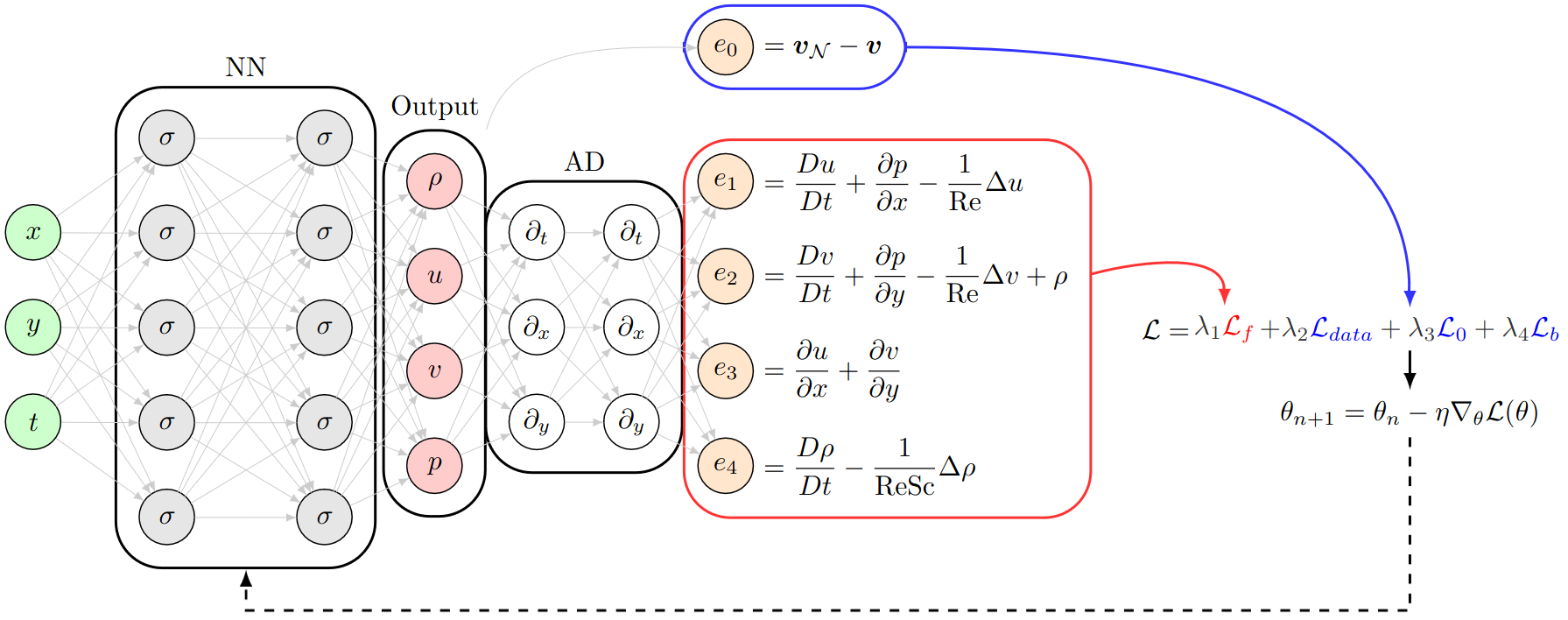
Figure 1: Physic informed neural network structure for gravity currents governing equations: a fully connected neural network take as input $(\textrm{{x}},t)\in\mathbb{R}^{3}$ and predicts $\bm{v}_{\mathcal{N}}(\textrm{{x}},t)=(\rho_{\mathcal{N}},u_{\mathcal{N}},v_{\mathcal{N}},p_{\mathcal{N}})$. The residuals of the governing equations $e_{1,\dots,4}$ are computed by automatic differentiation and $e_{0}$ denotes the mismatch between the observational data $\bm{v}$ and the predictions $\bm{v}_{\mathcal{N}}$, which are combined in the loss function $\mathcal{L}_{0},\mathcal{L}_{b}$ and $\mathcal{L}_{\textrm{data}}$. Finally, the weights and biases of the network are updated iteratively with gradient descent.

2 Governing equations of Lock-Exchange gravity currents

In the lock exchange flow (Shin et al. (2004)), fluids of different densities initially at rest are separated by a vertical membrane, in a tank. The fluids in the left and right hand compartments have the respective densities $\tilde{\rho_{1}}$ and $\tilde{\rho_{2}}$ with $\tilde{\rho_{1}}>\tilde{\rho_{2}}$, the density gradient is caused for instance by salinity difference. Once the membrane is withdrawn the density difference $\Delta\rho=\tilde{\rho_{1}}-\tilde{\rho_{2}}$ between the two compartments induces the generation and propagation of a gravity current at the tank bottom. The intensity of turbulent structures and induced mixing in the current is controlled by the Reynolds number $Re$. The flow is governed by Navier-Stokes, mass transport and incompressibility equations. Moreover, in this paper, we study Gravity Currents induced by small difference in density, so that Boussinesq Aproximation (Gray and Giorgini (1976)) is effective.

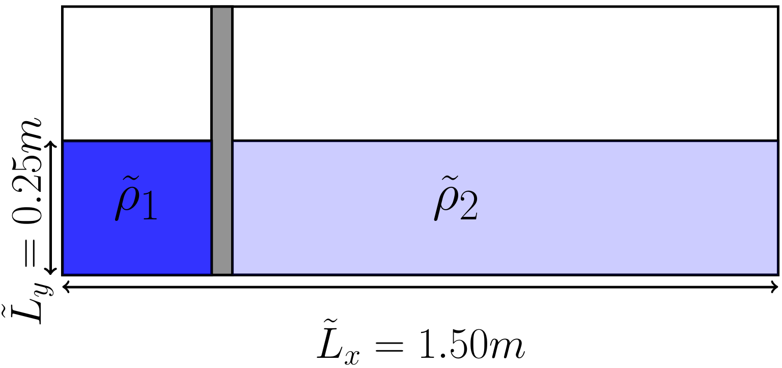
(a) Lock exchange tank : The lock-exchange configuration. At the initial moment, the wall is removed and the system evolves under the action of gravity only. The difference of density is achieved by a difference of salinity.

In order to render the equations dimensionless (see  Hartel et al. (2000)), we use $\tilde{L}_{y}$ as the characteristic length scale and the characteristic velocity is the buoyancy velocity defined as :

$$\tilde{u}_{b}=\sqrt{g\frac{\tilde{\rho_{1}}-\tilde{\rho_{2}}}{\tilde{\rho_{a}}}\tilde{L}_{y}},\quad\text{with}\quad\tilde{\rho}_{a}=\frac{\tilde{\rho_{1}}+\tilde{\rho_{2}}}{2}.$$ (7)

We consider small density difference $\tilde{\rho}_{1}-\tilde{\rho}_{2}\ll\tilde{\rho}_{1}$ for which the Boussinesq approximation can be adopted, thus the governing equations read in dimensionless form :

$$\dfrac{\partial\bm{u}}{\partial t}+(\bm{u}\cdot\nabla)~{}\bm{u}+\dfrac{\partial p}{\partial x}-\dfrac{1}{Re}\nabla^{2}\bm{u}+\rho~{}\bm{e_{y}}=0,$$ (8a)

$$\dfrac{\partial\rho}{\partial t}+(\bm{u}\cdot\nabla)~{}\rho-\dfrac{1}{Re\,Sc}\nabla^{2}\rho=0,$$ (8b)

$$\nabla\cdot\bm{u}=0,$$ (8c)

where $\bm{u}=(u,v)^{\intercal}$ denotes the dimensionless velocity vector. The non-dimensional pressure $p$ and density $\rho$ are given by :

$$p=\frac{\tilde{p}}{\tilde{\rho}_{a}\tilde{u}_{b}^{2}},\quad\rho=\frac{\tilde{\rho}-\tilde{\rho}_{2}}{\tilde{\rho_{1}}-\tilde{\rho_{2}}}.$$ (9)

The Reynolds number $Re$ and the Schmidt number $Sc$ arising in the dimensionless equations (8) are defined by :

$$Re=\frac{\tilde{u}_{b}\tilde{L}_{y}}{\tilde{\nu}},\quad Sc=\frac{\tilde{\nu}}{\tilde{\kappa}},$$ (10)

where $\tilde{\nu}$ is the kinematic viscosity and $\tilde{\kappa}$ denotes the molecular diffusivity of the chemical specie producing the density difference.

3 Application of PINNs on synthetical data

3.1 synthetic data for the lock-exchange problem

An accurate representation of the interface between the miscible fluids is crucial in gravity currents simulations, which requires high-order numerical methods to compute steep gradients in the vicinity of the interface. To this end, the governing equations (8) are solved with the code Nek5000 (Fischer et al. (2008)) that has been for example successfully employed in numerical investigations by  Özgökmen et al. (2004). The discretization scheme in Nek5000 is based on the spectral element method proposed by  Patera (1984) with exponential convergence in space and $3^{\text{rd}}$-order timestepping scheme.

We consider the dimensionless computational domain $\Omega=[0,6.0]\times[0,1.0]$ and $T=[0,10]$ with $Re=5500$. While for liquids such as salt water $Sc\simeq 700$, we consider here $Sc=1$. This assumption is commonly made to reduce computational costs and has low influence on the gravity current front as shown by  Marshall et al. (2021). A free-slip condition (no normal flow) is applied at $y=1.0$ and no slip-conditions are applied on the remaining domain boundaries. Grid independent results were obtain on a computational mesh of $90\times 45$ elements where unknowns are represented by $7^{\text{th}}$-order Lagrange interpolating polynomials, and with a fixed timestep $\Delta t=2.10^{-2}$ giving a Courant–Friedrichs–Lewy number less than $0.5$. We show in Fig. 3 the time evolution of the density field obtain with Nek5000.

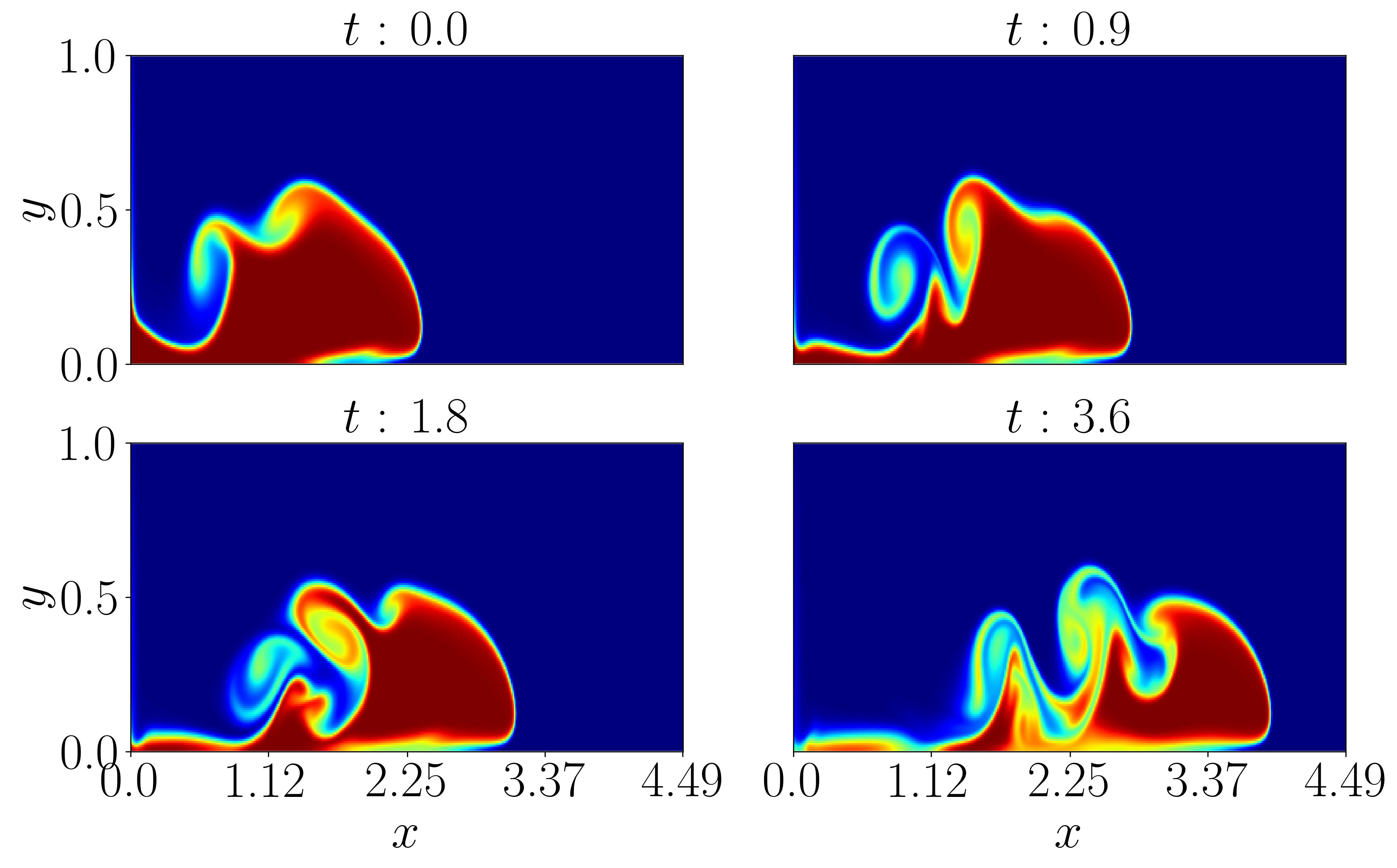
Figure 3: Heatmap of the density field $\rho$ for different time steps during the flow.

We build from this simulation a training dataset $\mathcal{D}$ where the collocation points are selected in the sub domain : $\Omega_{obs}\times T_{obs}=[0.0,4.5]\times[0,1.0]\times[4.0,7.5]\subset\Omega\times T$, which is discretized into a uniform Cartesian grid of $N_{x}\times N_{y}\times N_{t}$ points , where $N_{x}=750$, $N_{y}=150$ and $N_{t}=400$.

Finally, to mimic experimental measurements of LAT, we extract from this simulation the observed quantity of the density $\rho$ on each collocation points, and build our training dataset $\mathcal{D}=(\textbf{{x}}_{i},t_{i},\rho_{i})_{i=1\dots N_{x}N_{y}N_{t}}$ while the other fields $u,~{}v,~{}p$ are used for validation purpose.

3.2 Noise robustness

In this section, noises of varying magnitudes were added to $\mathcal{D}$. We investigate 4 different cases :

• Case 1 : Original dataset $\mathcal{D}$.

• Case 2 : We add a gaussian noise to $\rho$ field with standard deviation $\sigma=5\%$ (experimental precision of LAT).

• Case 3 : same as Case 2 but with $\sigma=25\%$.

• Case 4 : Same as case 3 but in addition, we remove a part of the information in all the snapshots. (we draw 200 squares of $10\times 10$ pixels randomly from Case 3 dataset ).

A visualization of training data for $\rho$ for cases 1-4 is available Fig. 4

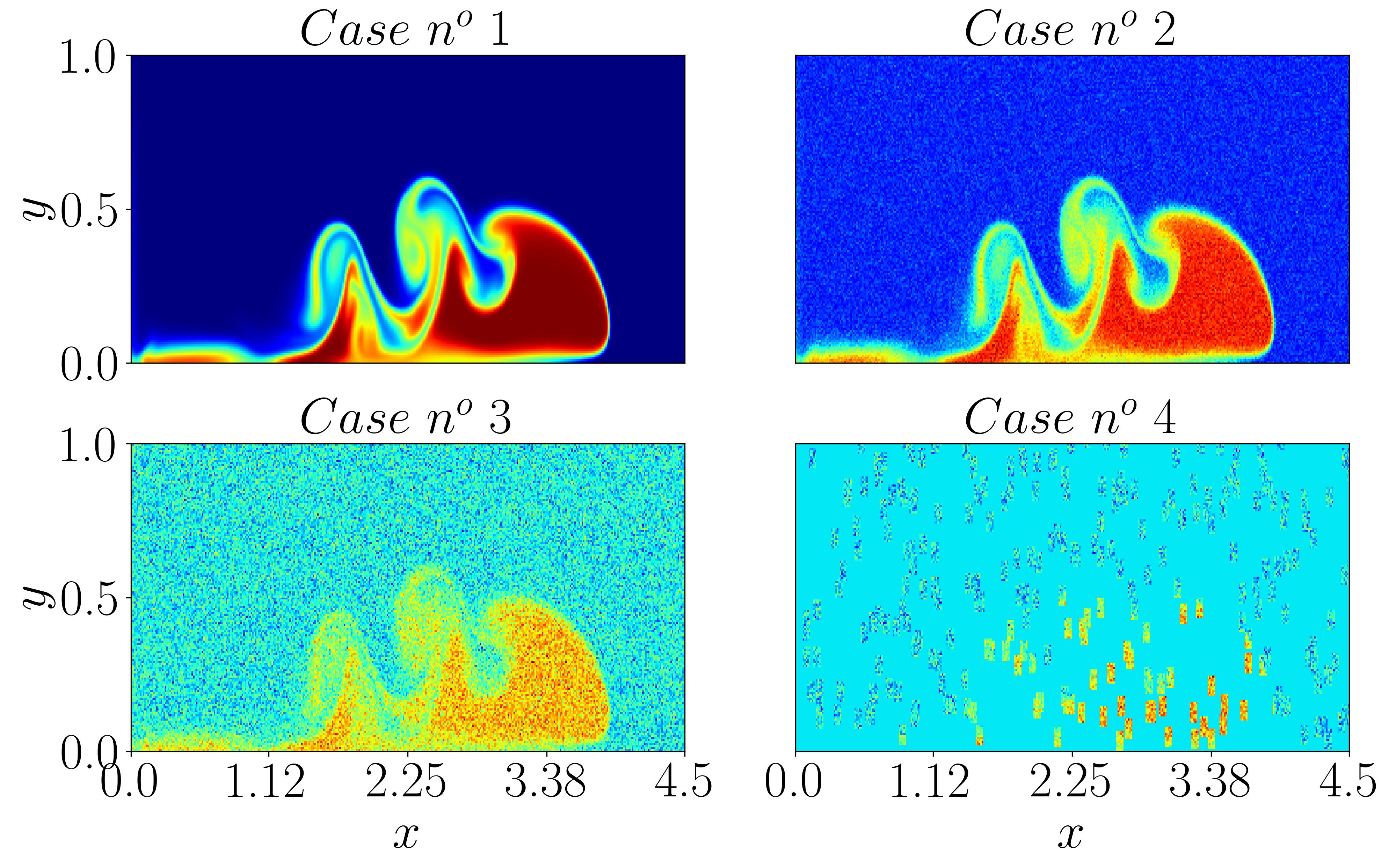
Figure 4: Density field at t = 10 for the different cases studied. In case number 4, 200 squares of size 10 by 10 are randomly selected in the mesh $\Omega_{obs}$

For all cases, the PINN loss function is expressed as:

$$\mathcal{L}=\lambda\mathcal{L}_{\textrm{data}}+\mathcal{L}_{f}$$ (11a)

$$\mathcal{L}_{f}=\dfrac{1}{N_{f}}\sum_{i=1}^{N_{f}}||f(\textrm{{x}}^{f}_{i},t^{f}_{i})||^{2}$$ (11b)

$$\mathcal{L}_{\textrm{data}}=\dfrac{1}{N_{\textrm{data}}}\sum_{i=1}^{N_{\textrm{data}}}||\rho_{\mathcal{N}}(\textrm{{x}}^{\textrm{data}}_{i},t^{\textrm{data}}_{i})-\rho(\textrm{{x}}^{\textrm{data}}_{i},t^{\textrm{data}}_{i})||^{2}$$ (11c)

The neural networks $\mathcal{N}$ take as input $(\textbf{{x}},t)=(x,y,t)$ and outputs the prediction $\bm{v}_{\mathcal{N}}(\textbf{{x}},t)=(\rho_{\mathcal{N}},u_{\mathcal{N}},v_{\mathcal{N}},p_{\mathcal{N}})$. The term $\mathcal{L}_{f}$ penalizes the governing equations  (8) and $\mathcal{L}_{\textrm{data}}$ penalizes mismatch between network prediction for $\rho_{\mathcal{N}}$ and observed $\rho$. The parameter $\lambda$ is a weighting coefficient used to reinforce the influence of 11c, in practice we set $\lambda=500$.

The neural network is composed of 8 layers of 190 neurons each. The stochastic Adam optimizer Kingma and Ba (2014) is employed for solving 2 : Glorot normal initializer Glorot and Bengio (2010) is employed to initialize the biases and the weights that are computed iteratively with a gradient update 3 on a subset $\mathcal{B}\subset\mathcal{D}$ called a batch. One training round over $\mathcal{D}$ is called an epoch. Training is done for 100 epochs with a batch size of 4096. We use a decreasing learning rate schedule. The learning rate starts at 1e-3 and ends at 1e-5. swish activation function Ramachandran et al. (2017) is selected for all layers except the last one. Finally, training is done with two GPU A6000 in parallel. The choice of these hyperparameters provides a goodsatisfactory compromise between quality of the results and computation time.

3.3 Results on synthetical data

For quantitative results, we define the following relative L2-norm :

$$\epsilon_{V}=\frac{100}{\sup_{\mathbf{x}\in\Omega_{obs}\times T_{obs}}\left|V_{\mathbf{x}}\right|}\sqrt{\frac{\sum_{\mathbf{x}\in\mathbf{X}}\left|V_{\mathcal{N}}(\mathbf{x})-V_{\mathbf{x}}\right|^{2}}{\left|\mathbf{X}\right|}}$$ (12)

where $V\in(\rho,u,v,w,p)$ and $\mathbf{X}\subseteq\Omega_{obs}\times T_{obs}$ defines the domain where the error is computed. We choose $\sup_{\mathbf{x}\in\Omega_{obs}\times T_{obs}}\left|V_{\mathbf{x}}\right|$ as reference value to avoid the division near to zero issue reported in Delcey et al. (2023).

In Fig. 5, we can see that the models for cases 1,2 and 3 are very efficient and accurate for the inference of all fields. Case 4 also performs great mostly everywhere, but we can see a big drop in performance near $x=1.5$ which may be due to a lack of training data in this area. For all the cases, the results for $u$ and $v$ close to $x=4.49$ are less accurate, but the steep variations near the front are well inferred.

Fig. 6 shows the evolution in time of the error in $\Omega_{obs}$ for the fields $\rho,~{}u,~{}v$. We can see the $L_{2}$-errors for the density and pressure field are almost constant in time except for density in Case 4. For all cases, the accuracy of the predictions $u$ and $v$ improves with time. Since gravity currents propagate from left to right, at the initial stages of the flow, a large portion of the area covered by the flow contains zero values that might not be useful for training the neural network, making it more challenging to effectively learn and approach the velocity. However, as the gravity current progresses and reaches the end of the flow, the entire current is present in $\Omega_{obs}$, and more useful values such as non zero variations of density can be utilized by the neural network, possibly leading to improved performance.

Table 1 illustrates the global error for Cases 1 to 4 between the density, velocity and pressure fields predicted by PINN, and the corresponding ground thruth. The first three cases have highly accurate predictions , indicating that the model is robust to noise. Despite the higher errors in the fourth case, the predictions still fall within an acceptable range, suggesting that the model can handle incomplete data with high noise level.

These results are very promising and the robustness of PINNs to noise in the 2D lock exchange configuration suggests the potential of this framework for real experimental data.

In the following section, we apply the PINN model to experimental data obtained by LAT.

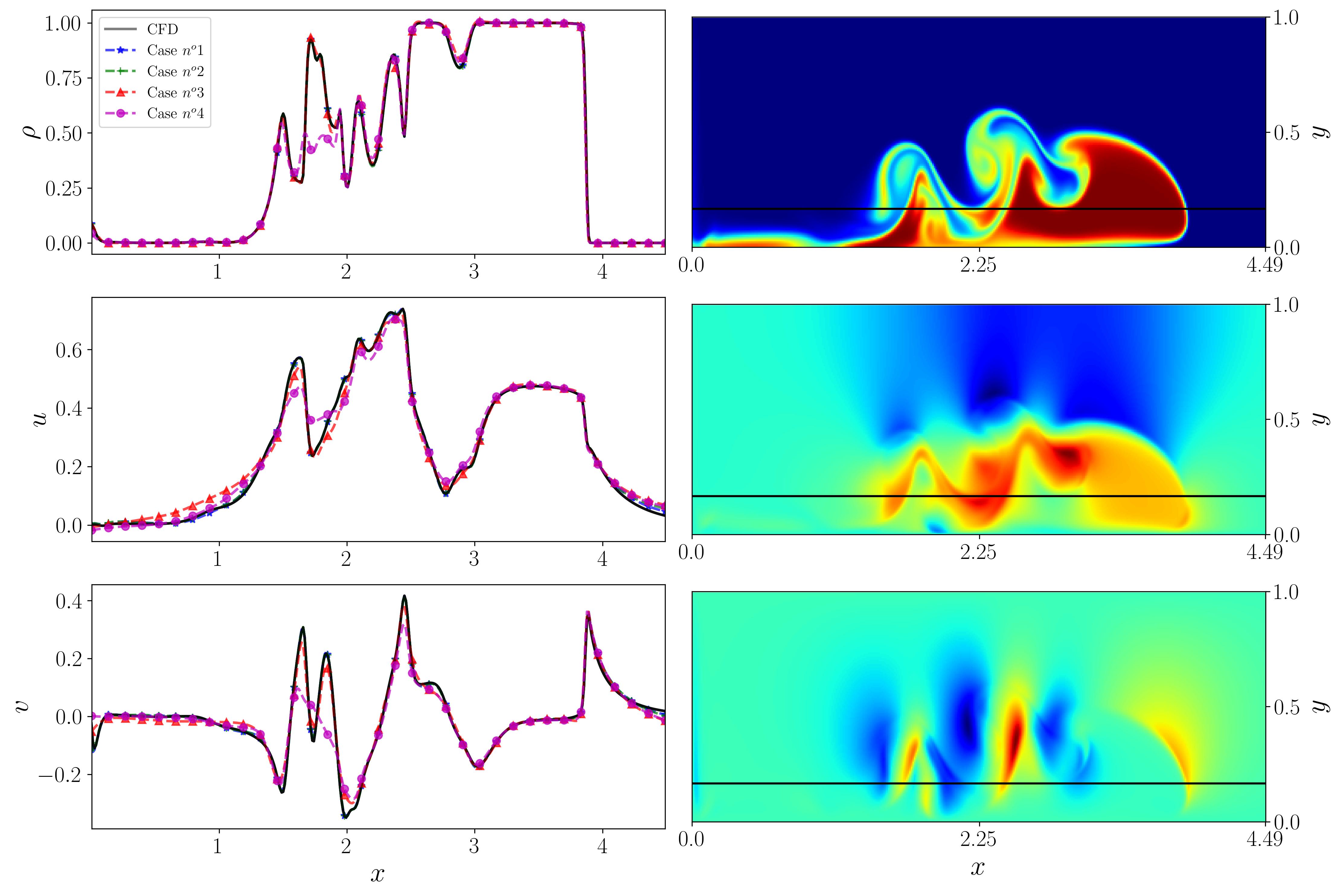
Figure 5: Horizontal profiles comparison. Profiles of $(\rho,u,v)$ reconstructed by PINNs for Cases 1-4 along the x-direction at y = 0.24 and t = 7.5 against the reference solution (first column). Corresponding location of the profile in $\Omega_{obs}$ (second column).

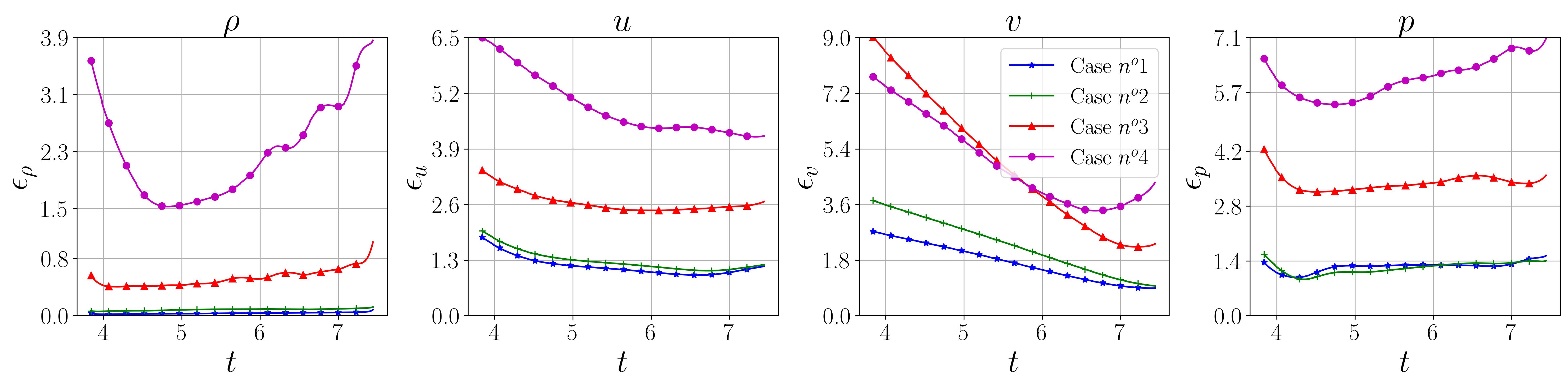
Figure 6: Evolution of the L2-relative error through time for density, velocity and pressure fields.

Case	$\epsilon_{\rho}$	$\epsilon_{u}$	$\epsilon_{v}$	$\epsilon_{p}$
Case $n^{o}$1	0.035%	1.17%	1.81%	1.03%
Case $n^{o}$2	0.085%	1.29%	2.41%	1.07%
Case $n^{o}$3	0.53%	2.65%	5.30%	2.48%
Case $n^{o}$4	7.98%	4.93%	5.12%	4.48%

Table 1: Relative $L_{2}$-norm errors of the fields reconstructed by PINN computed on the spatio-temporal domain $\Omega_{obs}\times T_{obs}$.

4 Application of PINNs to LAT experimental measurements

4.1 Experimental setup

The experimental apparatus is summarized in Fig. 7. Experiments are conducted in a $150$ cm long, $10$ cm wide and $35$ cm high plexiglas tank. After the tank is filled with freshwater to an height $25$ cm, a gate with insulating sides is inserted at 20 cm from the left end of the tank.

Salt is dissolved in the lock to reach a homogeneous density $\tilde{\rho}_{1}=1001.2~{}\textrm{kg.m}^{-3}$ slightly larger than the freshwater density $\tilde{\rho}_{2}=999.8~{}\textrm{kg.m}^{-3}$ which gives us $\Delta\rho=1.4~{}\textrm{kg.m}^{-3}$, $Re=14000$ and $Sc=1000$ according to the definitions in section (10).

Measurements are performed using two cameras and two light sources. The PIV and LAT cameras are respectively mounted with a $180$ mm f2-8 and $25$ mm lens. The cameras are mounted on tripods and placed at a distance of $250$ cm from the tank. Images are recorded at a frame rate of $10$ fps and the spatial resolution of the raw images is 8Mpx for both cameras.

The PIV (particle image velocimetry Raffel et al. (2007)) camera is synchronized with a vertical LASER sheet that illuminates the central section of the tank, providing two-dimensional vertical velocity field measurements as commonly performed in stratified flows.

The LAT (light attenuation technique) camera is synchronized with a white LED panel place behind the tank. The latter technique allows to measure high resolution cross-averaged density fields by adding a known concentration of tracer in the dense compartment. In the present experiment, a red food dye is used as a tracer for salinity and hence density. The reader may refer to Dossmann et al. (2016) for a detailed description of the LAT protocol.

The two cameras and light sources are computer
-controlled, which permits to synchronize velocity and density measurements. As the LED panel interferes with the PIV measurements, it is required to trigger the PIV and LAT sources in a slightly phase-shifted manner. Measurements are latter recombined on an identical timestep during the PIV post-process. A common spatial origin is used to match the recorded velocity and density field.

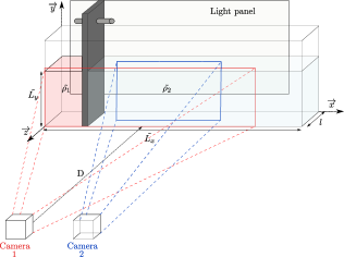
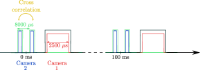
Figure 7: (a) Sketch of the experimental setup, including the tank, barrier, light panel, fluids and cameras 1 (LAT) and 2 (PIV). Combination of LAT and PIV measurement devices with $\tilde{L_{y}}$ = 25 cm, $\tilde{L_{x}}$ = 150 cm and l = 10 cm. The cameras are located at a distance of $D$=250 mm from the tank. (b) Time scale used to represent, in chronological order, the duration of PIV time with 8000 $\mu s$ correlation time between two images and LAT time with 2500 $\mu s$ exposure time.

As the studied flow evolves in 3D, using the canonical PINN model would imply forcing a neural network to impose the Navier-Stokes equations in 3D and having available measurements of the density field in the whole tank which is prohibitive in our case.

So in the following, we assume that the flow is homogeneous in the z-direction, this assumption is commonly made for the lock release configuration La Rocca and Bateman (2010). As a consequence, we reduce the problem size and consider only the 2D Navier-Stokes equations 8 and, under this assumption, the spanwise-averaged density $\overline{\rho}$ measured by LAT is assimilated to 2D density measurements $\rho$. In Fig. 8, we can see a sample of the fields measured by the combination of LAT and PIV.

4.2 Training data

The data are acquired on the spatial and temporal dimensionless domain $\Omega_{exp}\times T_{exp}=[3.0,4.65]\times[0.05,0.5]\times[19.5,21.5]$.

this domain is discretized into a uniform grid of $N_{x}\times N_{y}\times N_{t}$ points , where $N_{x}=1050$, $N_{y}=300$ and $N_{t}=90$.

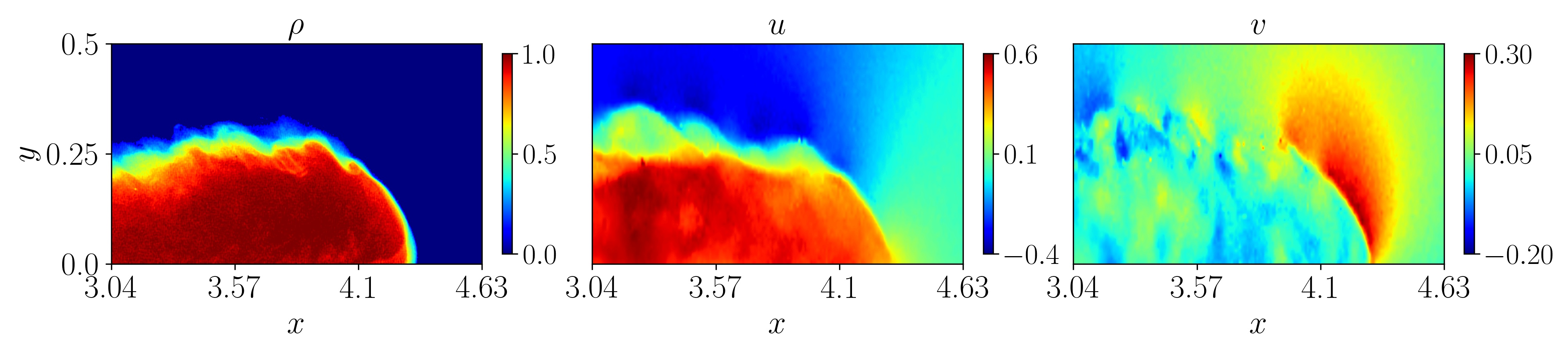
Figure 8: measures of density at $t=20.45$ and two components of velocity at $t=20.80.~{}~\rho$ is measured by LAT and $(u,v)$ are measured by PIV in the middle plane of the tank

Our objective is to infer the hydrodynamic field in the middle plane of the domain given LAT measurements of density. We keep the available PIV measurements for validation purpose.

We apply canonical PINN method with LAT experimental measures as observation data in the domain $\Omega_{exp}\times T_{exp}$ with Navier-Stokes equation 8 and loss fonction 11.

The neural network is composed of 8 layers of 250 neurons each which, in our case is the structures which gives the best results. Training is done for 150 epochs with a batch size of 4096. We use Adam optimizer with a decreasing learning rate schedule. The learning rate starts at 5e-4 and ends at 1e-5. Finally we use $swish$ activation function on each layers transition, except for the last layers where no activation function is selected.

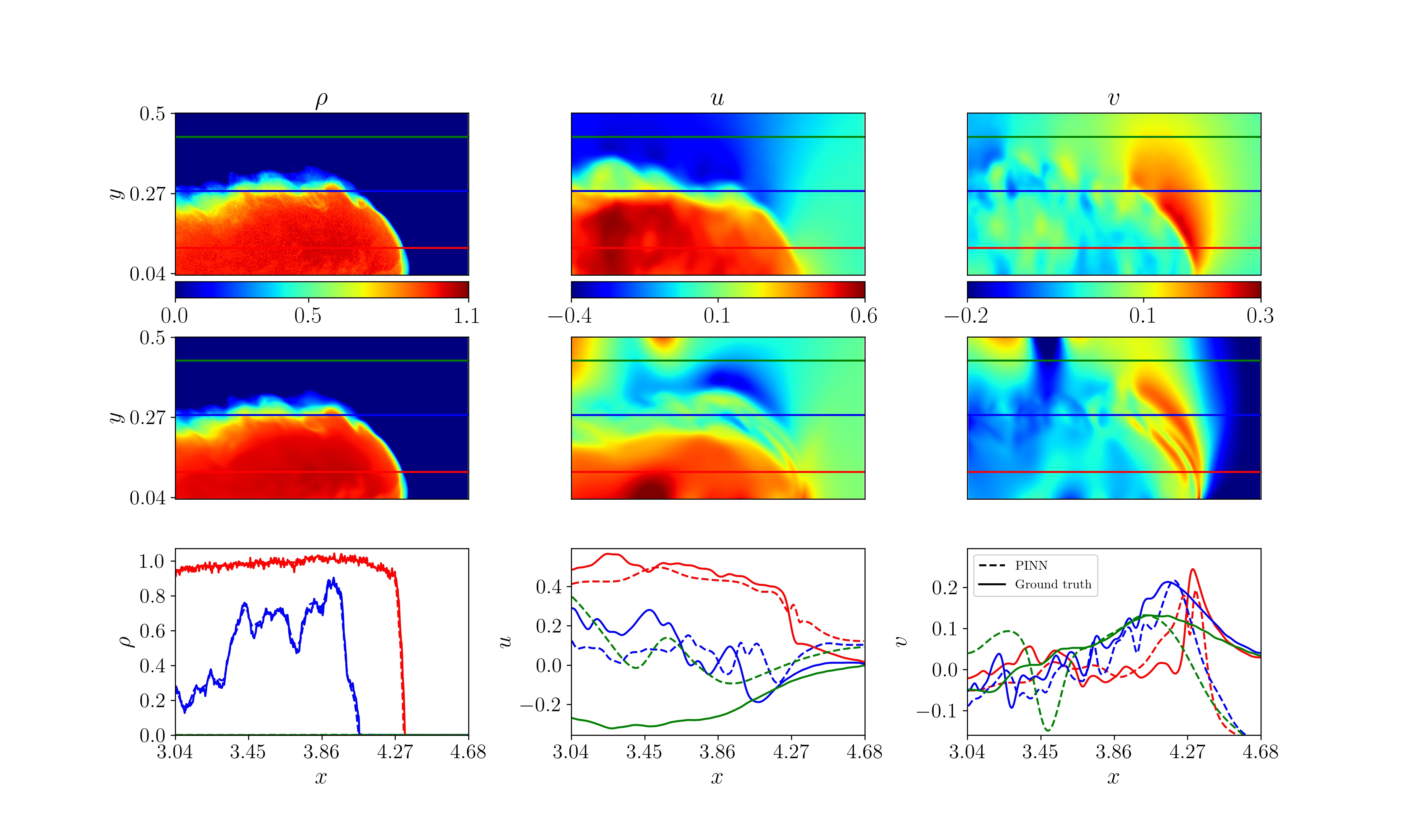
Figure 9: Comparison between measured and predicted density and velocity for model $\mathcal{N}$ at $t=20.8$. First line refers to $\rho$ obtained by LAT and $(u,v)$ measured by PIV . Second line refers to corresponding fields inferred by PINN , and third line corresponds to horizontal profiles along x-axis for $y=0.11$ (red), $y=0.28$ (blue) and $y=0.48$ (green) for both inferred and measured fields.

4.3 Results on experimental data

In Fig 9, we can see a comparison between predicted $\rho$ $u$ and $v$ fields and the corresponding measured fields by LAT/PIV. Since the model is trained on density, it is not surprising that the predicted density values are highly accurate, but we can notice that PINN has a smoothing effect on the density field. What is the most interesting here is the comparison on the velocity fields. Indeed, the NN has succeeded without prior information on $u$ and $v$ to reproduce the right amplitudes of values as well as the location of the current front. On the other hand, there is a bias in the values for $u$ and the small variations above the current (blue profile) are poorly captured. Moreover, for $v$, the values on the right of the front seem to be outliers.

After a thorough study of the problem parameters, we came to the conclusion that the residual related to the continuity equation (8c) in 2D degraded the results. So, to account for the spanwise variations of the flow, we propose a modification of the continuity equation (8c) :

$$~{}~{}~{}~{}~{}~{}~{}~{}~{}~{}~{}~{}~{}~{}~{}~{}~{}~{}~{}~{}\frac{\partial u}{\partial x}+\frac{\partial v}{\partial y}+\xi=0$$ (13)

where $\xi$ which depends on $(x,y,t)\in\Omega_{exp}\times T_{exp}$ is a new output of the neural network. Thus, the new model $\mathcal{M}$ take as input $(\textbf{{x}},t)=(x,y,t)$ and outputs the prediction $\bm{v}_{\mathcal{M}}(\textbf{{x}},t)=(\rho_{\mathcal{M}},u_{\mathcal{M}},v_{\mathcal{M}},p_{\mathcal{M}},\xi_{\mathcal{M}})$. Since the 3D Navier-Stokes equations involve $\dfrac{\partial w}{\partial z}$ in the continuity equation, we expect $\xi_{\mathcal{M}}$ to converge during training to the restriction of $\dfrac{\partial w}{\partial z}$ to the PIV plane. In the following, we denote by $\mathcal{N}$ or $\mathcal{M}$ either if the model was trained with the equation (8c) or with (13).

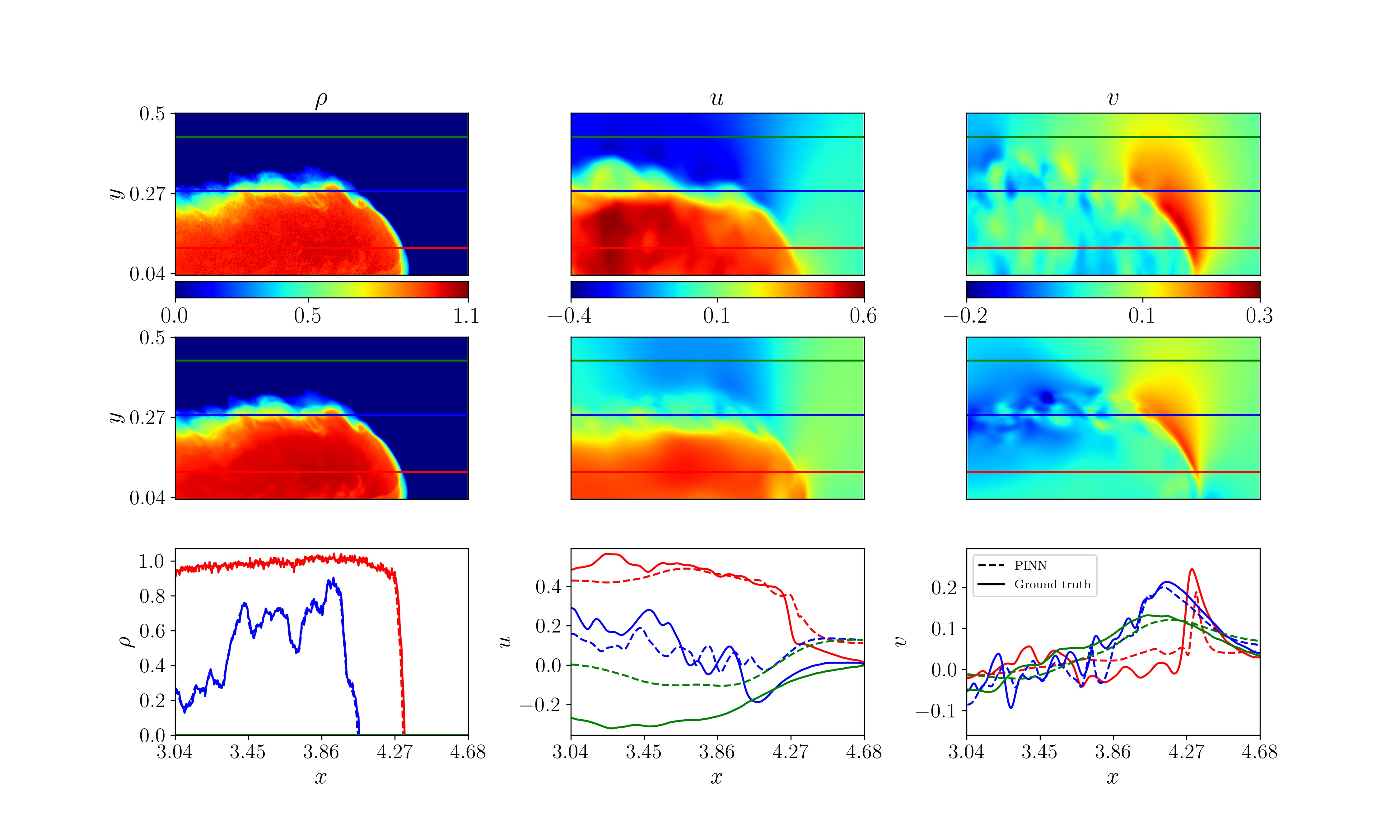
Figure 10: Comparison between measured and predicted density and velocity for model $\mathcal{M}$ at $t=20.8$. at $t=20.8$. First line refers to $\rho$ obtained by LAT and $(u,v)$ measured by PIV . Second line refers to corresponding fields inferred by PINN , and third line corresponds to horizontal profiles along x-axis for $y=0.11$ (red), $y=0.28$ (blue) and $y=0.48$ (green) for both inferred and measured fields.

The modification made to the equation has led to significant improvements in the accuracy of the predictions. The results Fig. 10 show the efficiency of this new formulation of the problem. For the $u$ component of velocity, although a small bias can still be observed on the values above the stream, the predicted quantities inside the stream and near the blue zone are suitable. The predicted profiles for the $v$ component of velocity in the blue and green zones are now accurate, and the model is able to capture steep variations, such as the large peak at $x=4.3$, with good accuracy.

Model	$\epsilon_{\rho}$	$\epsilon_{u}$	$\epsilon_{v}$
$\mathcal{N}$	1.72%	20.90%	31.5%
$\mathcal{M}$	1.35%	14.6%	12.65%

Table 2: Relative $L_{2}$-norm errors on the spatio-temporal domain $\Omega_{exp}\times T_{exp}$ between reconstructed and measured fields. model name is $\mathcal{N}$ or $\mathcal{M}$ either if training was done with standard continuity equation (8c) or variation (13)

The table 2 shows the overall improvement in predictions brought by the simple change in the continuity equation 13. The model achieve great results on the global space $\Omega_{exp}\times T_{exp}$.

Model $\mathcal{M}$ doesn’t take into account all the 3D effects, but correction (13) makes it more precise. The surrogate model is fully differentiable and enables the computation of various quantities of interest, including vorticity, pressure, and energy fluxes and budgets. In the following, we examine the pressure field inferred by analyzing energy fluxes and the residual of the energy conservation equation given by :

$$\left|e_{5}\right|=\bigg{|}\frac{\partial}{\partial t}\left(\frac{|\bm{u}|^{2}}{2}\right)+\nabla\cdot\left[\left(\dfrac{|\bm{u}|^{2}}{2}+p\right)\bm{u}\right]$$ (14)

$$-\nabla\cdot(\dfrac{1}{\textrm{Re}}\nabla\bm{u}\cdot\bm{u})+\dfrac{1}{\textrm{Re}}\nabla\bm{u}:\nabla\bm{u}+\rho\bm{u}\cdot\bm{e_{y}}\bigg{|}.$$

In Fig. 11, we represent the quantity $J=p\bm{u}$ where $\bm{u}=(u,v)^{T}$, and respectively the isovalues of the separated components $pv$, $pu$ given by $\mathcal{M}$ at three different times during the flow. These quantities provide information about the energy flux within the gravity current.

We clearly evidence a zone where the current transfers energy to the surrounding fluid, which are the zone where $pv$ reach its maximum values in the right of the current front. In the same way, one identifies a zone where the current captures energy from the ambient fluid which are the zone of circulation above the current where $pu$ reach its minimum values. We can notice a very sharp transition between these two zones (red dotted line) where $pv$ changes sign. This criterion is consistent through time and represents a quantitative criterium to divide the density field in two parts, the front and the head of the current. In the last raw of Fig. 11 vorticity isovalues inferred $\omega$ are plotted and superposed to the energy flux vector field. We observe that the transition between the two previously identified zones is also associated with the appearance of re-circulation rolls where the mixing becomes efficient.

Although we have no direct experimental measurement of the pressure field for validation, it is interesting to discuss its relevance in regards to the energy conservation equation (see eq (14)). For that, we plot in Fig. 12 the magnitude of energy residual $\lvert e_{5}\rvert$ defined as:

We find that $\lvert e_{5}\rvert$ is around $3\times 10^{-2}$. This error is small from a physical point of view, especially considering the experimental errors of measurements for such unsteady flows but is significant from a mathematical point of view. This can be explained by the nature of the physical model used to model the flow here. Indeed, we use the 2D equations to train the neural network. This approximation is justified in view of the mainly two-dimensional character of the flow but the small fluctuations of the transverse component of the velocity can carry a non-negligible fraction of the energy which would explain a significantly high value of the residuals $e_{5}$. An improvement in the future would be to develop the same type of approach but using 3D flow reconstruction methods from 2D measurements (see Delcey et al. (2023)). The implementation of the 3D equations would then allow to significantly reduce the error on the energy transport equation.

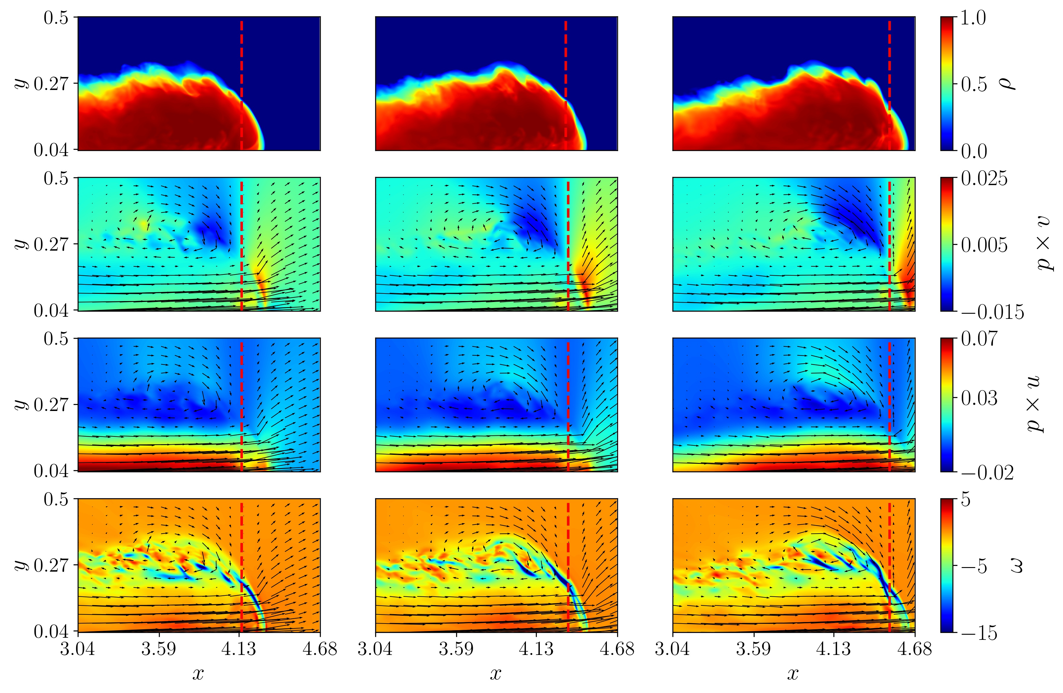
Figure 11: Energy flux and vorticity. Isovalues of $\rho$ (first line), $pu,pv$ (seconde and third line) and vorticity $\omega$ (fourth line) at times : $t=20.7,21.14$ and $21.6$ in addition in lines 2,3,4, the vector field $p\bm{u}$ is added.

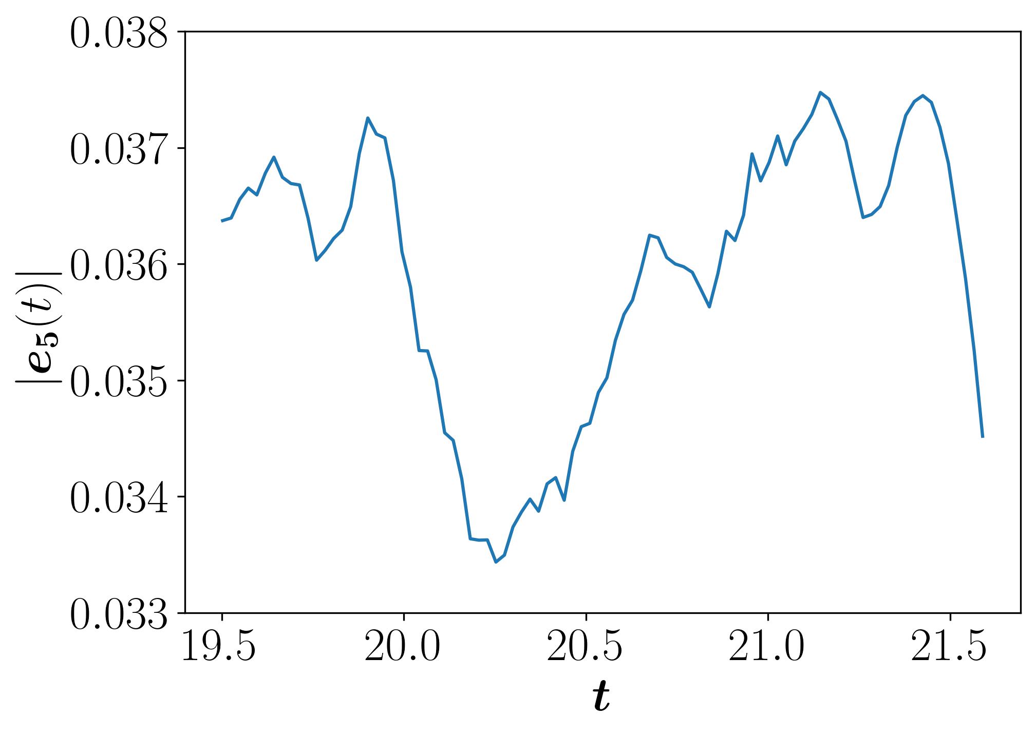
Figure 12: Time evolution of the residual of the energy equation (14).

5 Conclusion

In this work, we quantitatively demonstrate that PINNs are able to solve inverse problems from experimental data. We first investigated the robustness of this model to noisy and gappy data. This study was made from synthetic data obtained by the CFD solver Nek5000 for the lock-exchange configuration, and allowed us to study the parametric aspect of the model. Then we trained a physics informed model from LAT measurements acquired on the lock-exchange configuration, the inferred velocity fields have been compared to PIV measurements made simultaneously on the same experiment. Despite the assumption of homogeneity in z-direction, the results are convincing and the model succeeds in predicting the pressure field. Based on the energy flux computed from the results, we discuss the structure of the gravity current and show the potential of Physics Informed Neural Networks for ocean modeling.

6 Bibliography

References

- Perez-Diaz et al. (2018) B. Perez-Diaz, Palomar, et al., Piv-plif characterization of nonconfined saline density currents under different flow conditions, Journal of Hydraulic Engineering 144 (2018) 04018063.
- Crimaldi (2008) J. Crimaldi, Planar laser induced fluorescence in aqueous flows, Experiments in fluids 44 (2008) 851–863.
- Dossmann et al. (2016) Dossmann, et al., Experiments with mixing in stratified flow over a topographic ridge, Journal of Geophysical Research: Oceans 121 (2016) 6961–6977.
- Balasubramanian et al. (2018) Balasubramanian, et al., Entrainment and mixing in lock-exchange gravity currents using simultaneous velocity-density measurements, Physics of Fluids 30 (2018) 056601.
- Tian et al. (2003) Tian, et al., A 3d lif system for turbulent buoyant jet flows, Experiments in fluids 35 (2003) 636–647.
- Raffel (2015) M. Raffel, Background-oriented schlieren (bos) techniques, Experiments in Fluids 56 (2015) 1–17.
- Elsinga et al. (2006) G. E. Elsinga, et al., Tomographic particle image velocimetry, Experiments in fluids 41 (2006) 933–947.
- Partridge et al. (2019) Partridge, et al., A versatile scanning method for volumetric measurements of velocity and density fields, Measurement Science and Technology 30 (2019) 055203.
- Nash et al. (2005) Nash, et al., Estimating internal wave energy fluxes in the ocean, Journal of Atmospheric and Oceanic Technology 22 (2005) 1551–1570.
- Clark et al. (2010) Clark, et al., Generation, propagation, and breaking of an internal wave beam, Physics of Fluids 22 (2010). 076601.
- Allshouse et al. (2016) Allshouse, et al., Internal wave pressure, velocity, and energy flux from density perturbations, Physical Review Fluids 1 (2016) 014301.
- Fourés et al. (2014) Fourés, et al., A data-assimilation method for reynolds-averaged navier–stokes-driven mean flow reconstruction, Journal of Fluid Mechanics 759 (2014) 404–431.
- Mons et al. (2022) V. Mons, et al., Dense velocity, pressure and eulerian acceleration fields from single-instant scattered velocities through navier–stokes-based data assimilation, Measurement Science and Technology 33 (2022) 124004.
- Goodfellow et al. (2016) I. Goodfellow, et al., Deep Learning, MIT Press, 2016. http://www.deeplearningbook.org.
- Brunton et al. (2020) S. L. Brunton, et al., Machine learning for fluid mechanics, Annual review of fluid mechanics 52 (2020) 477–508.
- Raissi et al. (2020) M. Raissi, A. Yazdani, G. E. Karniadakis, Hidden fluid mechanics: Learning velocity and pressure fields from flow visualizations, Science 367 (2020) 1026–1030.
- Mao (2020) Mao, Physics-informed neural networks for high-speed flows, Computer Methods in Applied Mechanics and Engineering 360 (2020) 112789.
- Cai et al. (2021) Cai, et al., Physics-informed neural networks for heat transfer problems, Journal of Heat Transfer 143 (2021).
- Cuomo et al. (2022) Cuomo, et al., Scientific machine learning through physics-informed neural networks: Where we are and what’s next, Journal of Scientific Computing 92 (2022).
- Cai et al. (2021) Cai, et al., Flow over an espresso cup: inferring 3-d velocity and pressure fields from tomographic background oriented schlieren via physics-informed neural networks, Journal of Fluid Mechanics 915 (2021).
- Molnar et al. (2023) J. Molnar, et al., Estimating density, velocity, and pressure fields in supersonic flows using physics-informed bos, Experiments in Fluids 64 (2023) 14.
- Cybenko (1989) G. Cybenko, Approximation by superpositions of a sigmoidal function. math cont sig syst (mcss) 2:303-314, Mathematics of Control, Signals, and Systems 2 (1989) 303–314.
- Higham et al. (2019) Higham, et al., Deep learning: An introduction for applied mathematicians, Siam review 61 (2019) 860–891.
- Géron (2019) A. Géron, Hands-on machine learning with Scikit-Learn, Keras, and TensorFlow: Concepts, tools, and techniques to build intelligent systems, O’Reilly Media, 2019.
- Paszke et al. (2019) Paszke, et al., Pytorch: An imperative style, high-performance deep learning library, 2019. URL: http://arxiv.org/abs/1912.01703, cite arxiv:1912.01703Comment: 12 pages, 3 figures, NeurIPS 2019.
- Griewank et al. (1989) A. Griewank, et al., On automatic differentiation, Mathematical Programming: recent developments and applications 6 (1989) 83–107.
- Kingma and Ba (2014) D. P. Kingma, J. Ba, Adam: A method for stochastic optimization, arXiv preprint arXiv:1412.6980 (2014).
- Shin et al. (2004) Shin, et al., Gravity currents produced by lock exchange, Journal of Fluid Mechanics 521 (2004) 1–34.
- Gray and Giorgini (1976) D. D. Gray, A. Giorgini, The validity of the boussinesq approximation for liquids and gases, International Journal of Heat and Mass Transfer 19 (1976) 545–551.
- Hartel et al. (2000) Hartel, et al., Analysis and direct numerical simulation of the flow at a gravity-current head. part 1. flow topology and front speed for slip and no-slip boundaries, Journal of Fluid Mechanics 418 (2000) 189–212.
- Fischer et al. (2008) P. F. Fischer, et al., nek5000 Web page, 2008. Http://nek5000.mcs.anl.gov.
- Özgökmen et al. (2004) Özgökmen, et al., Three-dimensional turbulent bottom density currents from a high-order nonhydrostatic spectral element model, Journal of Physical Oceanography 34 (2004) 2006–2026.
- Patera (1984) A. T. Patera, A spectral element method for fluid dynamics: laminar flow in a channel expansion, Journal of computational Physics 54 (1984) 468–488.
- Marshall et al. (2021) Marshall, et al., The effect of schmidt number on gravity current flows: The formation of large-scale three-dimensional structures, Physics of Fluids 33 (2021) 106601.
- Glorot and Bengio (2010) X. Glorot, Y. Bengio, Understanding the difficulty of training deep feedforward neural networks, in: Proceedings of the thirteenth international conference on artificial intelligence and statistics, JMLR Workshop and Conference Proceedings, 2010, pp. 249–256.
- Ramachandran et al. (2017) Ramachandran, et al., Searching for activation functions, arXiv preprint arXiv:1710.05941 (2017).
- Delcey et al. (2023) Delcey, et al., Physics-informed neural networks for gravity currents reconstruction from limited data, Physics of Fluids 35 (2023). 027124.
- Raffel et al. (2007) M. Raffel, C. Willert, s. wereley, J. Kompenhans, Particle Image Velocimetry: A Practical Guide, Experimental Fluid Mechanics, Springer Berlin Heidelberg, 2007. URL: https://books.google.fr/books?id=WH5w2TvK2bQC.
- La Rocca and Bateman (2010) M. La Rocca, A. Bateman, Experimental and Theoretical Modelling of 3D Gravity Currents, 2010. doi:10.5772/13251.