Competing effects in fourth-order aggregation-diffusion equations

Abstract.

We give sharp conditions for global in time existence of gradient flow solutions to a Cahn-Hilliard-type equation, with backwards second order degenerate diffusion, in any dimension and for general initial data. Our equation is the 2-Wasserstein gradient flow of a free energy with two competing effects: the Dirichlet energy and the power-law internal energy. Homogeneity of the functionals reveals critical regimes that we analyse. Sharp conditions for global in time solutions, constructed via the minimising movement scheme, also known as JKO scheme, are obtained. Furthermore, we study a system of two Cahn-Hilliard-type equations exhibiting an analogous gradient flow structure.

1. Introduction

In this manuscript we are interested in the mathematical analysis of the equation

$$\partial_{t}\rho=-\,\mbox{div}(\rho\nabla(\Delta\rho))-\chi\Delta\rho^{m},$$ (1.1)

where $m\geq 1$, and its extension to systems. We look for solutions of (1.1) in the set of probabity densities, $\rho\in L^{1}_{+}(\mathbb{R}^{d}):=\{\rho\in L^{1}({\mathbb{R}^{d}}):\rho\geq 0\}$, thus setting the mass to one in the sequel without loss of generality. The parameter $\chi>0$ measures the relative balance between aggregation, modelled by backwards degenerate diffusion, and repulsion, modelled by fourth-order diffusion. The case of general masses can be reduced to (1.1) with a suitable parameter $\chi$ upon a standard time rescaling and mass normalisation, cf. Remark 3.1.

Equation (1.1) is related to the classical thin-film equations from lubrication theory, cf. [42, 7, 54, 6, 28, 41] and the references therein. Starting from a conjecture of Hocherman and Rosenau, [42], the authors in [8] study well-posedness and finite-time singularities of Cahn-Hiliard-type equations, in one spatial dimension on bounded interval with periodic boundary conditions. More precisely, they analyse the family of equations of the form

$$\partial_{t}\rho=-(\rho^{n}\rho_{xxx})_{x}-(\rho^{m-1}\rho_{x})_{x},$$ (1.2)

proving that for nonnegative (weak) solutions, blow-up can only occur for $m\geq n+3$. The results in [42, 8] hold for general degenerate mobilities, as in [8, Conjectures 1,2]. Afterwards, several contributions to the analysis of the one dimensional problem have been made. Linear ins/stability of steady states for the one-dimensional periodic problem was analysed in [44, 58]. Using the dissipation of a suitable energy functional, the authors of [46] were able to further characterise the energy landscape distinguishing between local minima and saddles among periodic steady states. Stability of droplets steady states with a fixed contact angle for the one-dimensional periodic problem was further studied in [45].

The critical case $m=n+3$ in one dimension is analysed in [65], where blow-up in finite time can only happen above a certain critical mass identified thanks to a sharp Sz.-Nagy inequality, cf. [61, 52]. Existence of selfsimilar blow-up solutions of (1.2) is explored in [59] for the critical case $m=n+3$. In particular, for $n=1$, there exists a family of blowing-up symmetric selfsimilar solutions with zero contact angle. Further analysis of one-dimensional self-similar solutions, both expanding and blowing-up, for the critical cases of (1.2) has been done in [38, 37, 58].

The nonlinear Cahn-Hilliard-type equations (1.1) have also been recently proposed as approximations of nonlocal aggregation-diffusion models of the form

$$\frac{\partial\rho}{\partial t}=\Delta\rho^{s}+\mbox{div}(\rho\nabla(W\ast\rho)),\quad s\geq 1,$$ (1.3)

by truncation of the Fourier expansion of the interaction potential $W$, see [5]. This approximation has been rendered rigorous under certain assumptions on the interaction potential $W$ in [34].

The connection between aggregation-diffusion and Cahn-Hilliard equations has also been generalised to systems of aggregation-diffusion equations modelling tissue growth and patterning due to cell-cell adhesion [25]. The authors in [39] show that cell-sorting phenomena are kept for the resulting system of equations:

$$\partial_{t}\rho =-\mbox{div}\left(\rho\nabla\left(\kappa\Delta\rho+\alpha\Delta\eta+\beta\rho+\omega\eta\right)\right),$$ (1.4a)

$$\partial_{t}\eta =-\mbox{div}\left(\eta\nabla\left(\alpha\Delta\rho+\Delta\eta+\omega\rho+\eta\right)\right).$$ (1.4b)

The parameters in the model are such that $\beta,\omega\in\mathbb{R}$ and the matrix

$$A=\begin{pmatrix}\kappa&\alpha\\ \alpha&1\end{pmatrix},$$

is positive definite. We extend the theory developed for the one-species case (1.1) to construct solutions to the systems of equations (1.4). The nonlocal-to-local limit in the context of systems has also been studied rigorously in [21]. We also mention that different multi-species Cahn-Hilliard equations are considered in [36, 35, 33] and references therein.

Equation (1.1) can be interpreted as $2$-Wasserstein gradient flow of the (extended) energy functional

$$\mathcal{F}_{m}[\rho]=\begin{cases}\frac{1}{2}\displaystyle\int_{\mathbb{R}^{d}}|\nabla\rho(x)|^{2}\,\mathrm{d}x-\chi\mathcal{E}_{m}[\rho],&\rho\in\mathcal{P}^{a}(\mathbb{R}^{d}),\,\nabla\rho\in L^{2}(\mathbb{R}^{d}),\\ +\infty,&\mbox{otherwise},\end{cases}$$ (1.5)

as already noted in [58], being

$$\mathcal{E}_{m}[\rho]=\begin{cases}\displaystyle\int_{\mathbb{R}^{d}}\rho(x)\log\rho(x)\,\mathrm{d}x,\quad&m=1,\\ \frac{1}{m-1}\displaystyle\int_{\mathbb{R}^{d}}\rho^{m}\mathrm{d}x,&m>1.\end{cases}$$ (1.6)

This gradient flow structure was made rigorous for related Cahn-Hilliard equations in [51, 47]. However, the former does not include the second-order backwards diffusion term in (1.1), while the latter is concerned with more general, density-dependent, mobilities.

As for the multi-species case, by defining the free energy functional as

$$\tilde{\bm{\mathcal{F}}}[\rho,\eta]=\int_{{\mathbb{R}^{d}}}\left(\frac{\kappa}{2}|\nabla\rho|^{2}+\frac{1}{2}|\nabla\eta|^{2}+\alpha\nabla\rho\cdot\nabla\eta-\frac{\beta}{2}\rho^{2}-\frac{1}{2}\eta^{2}-\omega\rho\eta\right)\,\mathrm{d}x,$$

system (1.4) can be written as a 2-Wasserstein gradient flow with respect to the (extended) free energy functional

$$\bm{\mathcal{F}}[\rho,\eta]=\begin{cases}\tilde{\bm{\mathcal{F}}}[\rho,\eta]&\mbox{if }(\rho,\eta)\in\mathcal{P}^{a}(\mathbb{R}^{d})^{2},\,(\nabla\rho,\nabla\eta)\in L^{2}(\mathbb{R}^{d})^{2}\\ +\infty&\mbox{otherwise.}\end{cases}$$ (1.7)

Our main goal is to show global existence of weak solutions of (1.1) for $m<m_{c}:=2+\frac{2}{d}$ (subcritical case) and for $m=m_{c}$ (critical case) for subcritical mass, $0<\chi<\chi_{c}$, by leveraging the aforementioned gradient flow structure. The critical parameter $\chi_{c}$ is identified by the sharp constant of a suitable functional inequality [48]. The critical exponent $m_{c}$ is determined by scaling arguments using mass-preserving dilations of densities in the energy functional (1.5). Moreover, we also obtain global existence of weak solutions for the system (1.4) by an analogous approach. In fact, we employ the (by now) classical variational minimising movement scheme, or JKO scheme, [43, 1] to obtain an approximation of a candidate solution. A crucial step will be to use the flow interchange technique, developed in [51, 47], to gain suitable regularity. Afterwards, we check that limits of the variatonal scheme are indeed weak solutions in any dimension.

Our main result provides sharp conditions on the exponent of backwards diffusion in (1.1) to ensure global existence of solutions in the natural class of initial data for any dimension compared to previous literature [65, 58, 47, 49].

The key ingredient to take advantage of the gradient flow structure of (1.1) and system (1.4) is to have uniform bounds on the competing terms in the free energies (1.5) and (1.7), respectively. Interestingly, this is reminiscent of similar arguments developed for generalisations of the Patlak-Keller-Segel equation for chemotactic cell movement [10, 19, 24]. Actually, we can draw a nice parallelism with this well studied problem. Generalised Patlak-Keller-Segel equations are of the form (1.3). In particular, let us focus on the power-law kernel

$$W_{k}(x)=\begin{dcases}\frac{|x|^{k}}{k}&\text{if }k\neq 0,\\ \log|x|&\text{if }k=0.\end{dcases}$$

We find an immediate connection with the problem (1.1). Analogously to the case we are studying in this work, there exists a critical exponent, $s_{c}=1-\frac{k}{d}$, also found via mass-preserving dilations on the corresponding free energy functional which characterises the behaviour of (1.3).

The case $s>s_{c}$ is the diffusion dominated regime and global well-posedness for (1.3) is expected, see for instance [15, 60, 10, 16, 17, 23]. This is analogous to the case $1\leq m<m_{c}$ for (1.1).

As for the range $1\leq s<s_{c}$, aggregation-dominated regime for Eq. (1.3) — analogous to the case $m>m_{c}$ for (1.1) — coexistence of blow-up and global existence depending on the initial data is expected, see [50, 4, 27] for instance.

In the fair competition regime $s=s_{c}$ — analogous to our critical exponent $m=m_{c}$ — there exists a dichotomy between aggregation and diffusion in terms of the initial mass: $M$, analogous to our parameter $\chi$. Sharp constants of variants of Hardy-Littlewood-Sobolev type inequalities determine the critical value of the mass $M_{c}$ for (1.3), analogously to our critical parameter $\chi_{c}$. We note that for our fourth-order Cahn-Hilliard type equation, the crucial functional inequality was established in [48]. In the supercritical mass case, $M>M_{c}$, there exists solutions that blow-up in finite time, see for instance [10, 3, 4, 16, 17]. In the subcritical mass case, $M<M_{c}$, global existence of solutions is shown and spreading self-similar solutions are expected to attract the long time dynamics, see for instance [32, 11, 4, 3, 16, 17].

In the critical case $M=M_{c}$, there are infinitely many stationary states given by the optimisers of the variants of the HLS inequalities, solutions are globally well-posed blowing-up at infinite time for bounded second moment initial data, and local stability of stationary solutions is expected, see [32, 10, 9, 66, 16, 17].

We shall perform a parallel study to nonlinear Keller-Segel equations (1.3) for our family of Cahn-Hilliard equations (1.1), depending on the critical exponent case $m_{c}$ and parameter $\chi$.

Finally, we want to emphasize that our work sets the path to many other interesting open questions. Uniqueness is widely open being the functionals not convex, even in subsets, in any obvious manner. Existence of minimisers in the subcritical case in the whole space is not clear since we do not know at present how to bound uniformly in time the second moment or any other quantity controlling escape of mass at infinity. Long time asymptotics are, in turn, widely open in all global existence cases. Free boundary problem techniques could help understand if the evolution leads to compactly supported solutions corresponding to compactly supported initial data. This conjecture is corroborated by numerical experiments being this another challenging problem. In the two-species case, we can identify other interesting issues such as sharp segregation for specific parameter values between the two species not only at steady states but along their evolutions. This information is important for the applications in mathematical biology [25, 39].

We structure the paper as follows. Section 2 is devoted to the precise statements of the main theorems together with some preliminary material used in the sequel. We will analyse the existence of global minimisers of the energy (1.5) following the strategies in [32, 10, 16] in Section 3. In Section 4 we deal with the core main result of global existence of weak solutions to the single equation (1.1) in any dimension for generic initial data. Finally, Section 5 focuses on the generalisation of this approach to the case of systems of the form (1.4).

2. Main results and preliminaries

We begin by listing the main results covered in this manuscript. First we study some properties of the free energy functional $\mathcal{F}_{m}$ and its minimisers. The following theorem summarises the results proven in Section 3.

Theorem 2.1.

Let $\mathcal{F}_{m}$ be as in (1.5). The following holds:

1. If $1\leq m<2+2/d$, then $\mathcal{F}_{m}$ is bounded from below.

2. If $m=2+2/d$, then, for the subcritical and critical mass regimes, $\mathcal{F}_{m}$ is bounded from below. Furthermore, for the critical mass, the infimum is achieved. In the supercritical mass regime, $\mathcal{F}_{m}$ is unbounded from below.

3. If $m>2+2/d$, then $\mathcal{F}_{m}$ is unbounded from below.

Case $(1)$ is proven in 3.1. Case $(2)$ is a combination of two results. In 3.2 we show that for $\chi\leq\chi_{c}$ the free energy is bounded from below. In 3.3, we prove that the infimum is achieved for critical mass and that the free energy is unbounded if $\chi>\chi_{c}$. Finally, in 3.5 we show case $(3)$.

Throughout the manuscript, we denote by ${\mathcal{P}}({\mathbb{R}^{d}})$ the set of probability measures on ${\mathbb{R}^{d}}$, for $d\in\mathbb{N}$, and by ${\mathcal{P}}_{2}({\mathbb{R}^{d}}):=\{\rho\in{\mathcal{P}}({\mathbb{R}^{d}}):\mathrm{m}_{2}(\rho)<+\infty\}$, being $\mathrm{m}_{2}(\rho):=\int_{\mathbb{R}^{d}}|x|^{2}\,\mathrm{d}\rho(x)$ the $2^{\mathrm{nd}}$-order moment of $\rho$. We shall use ${\mathcal{P}}^{a}({\mathbb{R}^{d}})$ and ${\mathcal{P}}_{2}^{a}({\mathbb{R}^{d}})$ for elements in ${\mathcal{P}}({\mathbb{R}^{d}})$ and ${\mathcal{P}}_{2}({\mathbb{R}^{d}})$ which are absolutely continuous with respect to the Lebesgue measure.

The second result we prove is the existence of weak solutions to (1.1), in the following sense:

Definition 2.1 (Weak solution).

A weak solution to (1.1) on the time interval $[0,T]$, with initial datum $\rho_{0}\in{\mathcal{P}_{2}^{a}({\mathbb{R}^{d}})}$ such that $\nabla\rho_{0}\in L^{2}({\mathbb{R}^{d}})$, is a narrowly continuous curve $\rho:[0,T]\to{\mathcal{P}_{2}({\mathbb{R}^{d}})}$ satisfying the following properties:

1. $\rho\in L^{\infty}([0,T];L^{p}({\mathbb{R}^{d}}))\cap L^{\infty}([0,T];H^{1}({\mathbb{R}^{d}}))\cap L^{2}([0,T];H^{2}({\mathbb{R}^{d}}))$, for any $p\in[1,2^{*}]$, where $2^{*}=+\infty$ if $d=1,2$ and $2^{*}=2d/(d-2)$ if $d\geq 3$;

2. for every $\varphi\in C_{c}^{2}({\mathbb{R}^{d}})$ and every $0\leq s_{1}<s_{2}\leq T$ it holds

   $$\int_{{\mathbb{R}^{d}}}\varphi(x)\rho(s_{2},x)\,\mathrm{d}x =\int_{{\mathbb{R}^{d}}}\varphi(x)\rho(s_{1},x)\,\mathrm{d}x$$

   $$\quad-\int_{s_{1}}^{s_{2}}\int_{\mathbb{R}^{d}}\left(\rho\Delta\rho\Delta\varphi+\Delta\rho\nabla\rho\cdot\nabla\varphi\right)\,\mathrm{d}x\,\mathrm{d}t$$

   $$\quad-\chi\int_{s_{1}}^{s_{2}}\int_{\mathbb{R}^{d}}\rho^{m}\Delta\varphi\,\mathrm{d}x\,\mathrm{d}t.$$

Theorem 2.2.

Assume $1\leq m<2+2/d$ or $m=2+2/d$ with subcritical mass $\chi<\chi_{c}$ and let $\rho_{0}\in\mathcal{P}_{2}^{a}({\mathbb{R}^{d}})$ be an initial datum such that $\mathcal{F}_{m}[\rho_{0}]<+\infty$. Then there exists a weak solution to (1.1).

We extend our results from the one species case to construct weak solutions to system (1.4), in the following sense.

Definition 2.2 (Weak solution for the system).

A weak solution to (1.4) on the time interval $[0,T]$, with initial datum $\sigma_{0}=(\rho_{0},\eta_{0})\in{\mathcal{P}}_{2}^{a}({\mathbb{R}^{d}})^{2}$ such that $\nabla\rho_{0},\nabla\eta_{0}\in L^{2}({\mathbb{R}^{d}})$, consists of a pair of narrowly continuous curves $\rho,\eta:[0,T]\rightarrow{\mathcal{P}}_{2}({\mathbb{R}^{d}})$ satisfying the following properties:

1. $\rho,\eta\in L^{\infty}([0,T];L^{p}({\mathbb{R}^{d}}))\cap L^{\infty}([0,T];H^{1}({\mathbb{R}^{d}}))\cap L^{2}([0,T];H^{2}({\mathbb{R}^{d}}))$, for any $p\in[1,2^{*}]$, where $2^{*}=+\infty$ if $d=1,2$ and $2^{*}=2d/(d-2)$ if $d\geq 3$;

2. for every $\varphi,\psi\in C^{2}_{c}({\mathbb{R}^{d}})$ and every $0\leq s_{1}<s_{2}\leq T$ it holds

   $$\int_{{\mathbb{R}^{d}}}\varphi(x)\rho(s_{2},x)\,\mathrm{d}x =\int_{{\mathbb{R}^{d}}}\varphi(x)\rho(s_{1},x)\,\mathrm{d}x$$

   $$\quad-\kappa\int_{s_{1}}^{s_{2}}\int_{{\mathbb{R}^{d}}}\rho\Delta\rho\Delta\varphi+\nabla\rho\cdot\nabla\varphi\Delta\rho\,\mathrm{d}x\,\mathrm{d}t$$

   $$\quad-\alpha\int_{s_{1}}^{s_{2}}\int_{{\mathbb{R}^{d}}}\rho\Delta\eta\Delta\varphi+\nabla\rho\cdot\nabla\varphi\Delta\eta\,\mathrm{d}x\,\mathrm{d}t$$

   $$\quad-\frac{\beta}{2}\int_{s_{1}}^{s_{2}}\int_{{\mathbb{R}^{d}}}\rho^{2}\Delta\varphi\,\mathrm{d}x\,\mathrm{d}t+\omega\int_{s_{1}}^{s_{2}}\int_{{\mathbb{R}^{d}}}\rho\nabla\eta\cdot\nabla\varphi\,\mathrm{d}x\,\mathrm{d}t,$$

   $$\int_{{\mathbb{R}^{d}}}\psi(x)\eta(s_{2},x)\,\mathrm{d}x =\int_{{\mathbb{R}^{d}}}\psi(x)\eta(s_{1},x)\,\mathrm{d}x$$

   $$\quad-\int_{s_{1}}^{s_{2}}\int_{{\mathbb{R}^{d}}}\eta\Delta\eta\Delta\psi+\nabla\eta\cdot\nabla\psi\Delta\eta\,\mathrm{d}x\,\mathrm{d}t$$

   $$\quad-\alpha\int_{s_{1}}^{s_{2}}\int_{{\mathbb{R}^{d}}}\eta\Delta\rho\Delta\psi+\nabla\eta\cdot\nabla\psi\Delta\rho\,\mathrm{d}x\,\mathrm{d}t$$

   $$\quad-\frac{1}{2}\int_{s_{1}}^{s_{2}}\int_{{\mathbb{R}^{d}}}\eta^{2}\Delta\psi\,\mathrm{d}x\,\mathrm{d}t+\omega\int_{s_{1}}^{s_{2}}\int_{{\mathbb{R}^{d}}}\eta\nabla\rho\cdot\nabla\psi\,\mathrm{d}x\,\mathrm{d}t.$$

Theorem 2.3.

Let $(\rho_{0},\eta_{0})\in\mathcal{P}_{2}^{a}({\mathbb{R}^{d}})\times{\mathcal{P}_{2}^{a}({\mathbb{R}^{d}})}$ be an initial datum such that $\bm{\mathcal{F}}[\rho_{0},\eta_{0}]<+\infty$. Then there exists a weak solution to (1.4).

The last result is generalised to a wider class of systems allowing for nonlinear self-diffusion terms.

2.1. Preliminaries

We present the notation and we collect some a priori results that we will use throughout the manuscript.

A key tool for the analysis is the Wasserstein metric, that is a distance function in the space of probability measures with finite second order moments.

Definition 2.3 ($2$-Wasserstein distance).

For $\mu$, $\nu\in\mathcal{P}_{2}({\mathbb{R}^{d}})$, we define the $2$-Wasserstein distance, $\mathcal{W}_{2}(\mu,\nu)$, between $\mu$ and $\nu$ as

$$\mathcal{W}_{2}(\mu,\nu):=\min_{\gamma\in\Gamma(\mu,\nu)}\left\{\int_{{\mathbb{R}^{d}}\times{\mathbb{R}^{d}}}|x-y|^{2}\,\mathrm{d}\gamma(x,y)\right\}^{\frac{1}{2}},$$

where $\Gamma(\mu,\nu)$ is the set of transport plans between $\mu$ and $\nu$,

$$\Gamma(\mu,\nu)=\left\{\gamma\in\mathcal{P}({\mathbb{R}^{d}}\times{\mathbb{R}^{d}})\,:\,(\pi_{x})_{\#}\gamma=\mu,\,(\pi_{y})_{\#}\gamma=\nu\right\},$$

and $\pi_{x}$ and $\pi_{y}$ are the projections onto the first and the second variables respectively.

In the expression above, marginals are the push-forward of $\gamma$ through $\pi_{i}$. For a measure $\rho\in{\mathcal{P}}({\mathbb{R}^{d}})$ and a Borel map $T:{\mathbb{R}^{d}}\to{\mathbb{R}^{n}}$, $n\in\mathbb{N}$, the push-forward of $\rho$ through $T$ is defined by

$$\int_{{\mathbb{R}^{n}}}f(y)\,\mathrm{d}T_{\#}\rho(y)=\int_{{\mathbb{R}^{d}}}f(T(x))\,\mathrm{d}\rho(x)\qquad\mbox{for all $f$ Borel functions on}\ {\mathbb{R}^{d}}.$$

We refer the reader to [1, 57, 63] for further details on optimal transport theory and Wasserstein spaces.

In order to obtain strong convergence of $\rho$ in $L^{2}([0,T];L^{2}({\mathbb{R}^{d}}))$ we take advantage of a refined version of the Aubin-Lions Lemma for compactness in measures, due to Rossi and Savaré. It relies on two conditions: tightness and weak integral equi-continuity.

Proposition 2.1 ([55], Theorem 2).

Let $X$ be a separable Banach space and consider

• a lower semicontinuous functional $\mathcal{I}:X\rightarrow[0,+\infty]$ with relatively compact sublevels in $X$,

• a pseudo-distance $g:X\times X\rightarrow[0,+\infty]$, i.e. $g$ is lower semicontinuous and such that $g(\rho,\eta)=0$ for any $\rho,\eta\in X$ with $\mathcal{I}[\rho]<\infty$ and $\mathcal{I}[\eta]<\infty$ implies $\rho=\eta$.

Let $U$ be a set of measurable functions $u:(0,T)\rightarrow X$, with a fixed $T>0$. Assume further that $U$ is tight with respect to $\mathcal{I}$

$$\sup_{u\in U}\int_{0}^{T}\mathcal{I}[u(t)]\,\mathrm{d}t<\infty\,,$$ (2.1)

and satisfies the weak integral equi-continuity condition

$$\lim_{h\downarrow 0}\sup_{u\in U}\int_{0}^{T-h}g\left(u(t+h),u(t)\right)\mathrm{d}t=0\,.$$ (2.2)

Then $U$ contains an infinite sequence $(u_{n})_{n\in\mathbb{N}}$ convergent in measure, with respect to $t\in(0,T)$, to a measurable $\tilde{u}:(0,T)\to X$, i.e.

$$\lim_{n\rightarrow\infty}\left|\{t\in(0,T):\;\|u_{n}(t)-\tilde{u}(t)\|_{X}\geq\delta\}\right|=0,\quad\forall\delta\geq 0\,.$$ (2.3)

In addition to the strong convergence given by 2.1, we will need an $L^{2}$ bound on $\Delta\rho$ to obtain suitable compactness in time and space for $\nabla\rho$ and $\Delta\rho$. We employ the flow interchange technique, developed by Matthes, McCann and Savaré in [51] and previously used in [54] — we also refer the reader to [14, 20, 30, 31] for further details. The idea of the flow interchange consists in considering the dissipation of the free energy $\mathcal{F}_{m}$ along a solution of an auxiliary gradient flow, and using the Evolution Variational Inequality (EVI) afterwards to obtain the desired estimate. For the reader’s convenience we recall the definition of $\lambda$-flow for a general functional $\mathcal{G}$, which is connected to the EVI.

Definition 2.4 ($\lambda$-flow).

A semigroup $S_{\mathcal{G}}:[0,+\infty]\times\mathcal{P}_{2}({\mathbb{R}^{d}})\to\mathcal{P}_{2}({\mathbb{R}^{d}})$ is a $\lambda$-flow for a functional $\mathcal{G}:\mathcal{P}_{2}({\mathbb{R}^{d}})\to\mathbb{R}\cup\{\infty\}$ with respect to the distance $\mathcal{W}_{2}$ if, for an arbitrary $\rho\in\mathcal{P}_{2}(\mathbb{R}^{d})$, we have that the curve $t\mapsto S_{\mathcal{G}}^{t}\rho$ is absolutely continuous on $[0,\infty)$ and it satisfies the EVI

$$\frac{1}{2}\frac{\mathrm{d}^{+}}{\mathrm{d}t}\mathcal{W}_{2}^{2}(S_{\mathcal{G}}^{t}\rho,\mu)+\frac{\lambda}{2}\mathcal{W}_{2}^{2}(S_{\mathcal{G}}^{t}\rho,\mu)\leq\mathcal{G}[\mu]-\mathcal{G}[S_{\mathcal{G}}^{t}\rho],$$ (EVI)

for all $t>0$, with respect to every reference measure $\mu\in\mathcal{P}_{2}({\mathbb{R}^{d}})$ such that $\mathcal{G}[\mu]<\infty$.

As shown in the seminal work by Jordan, Kinderlehrer and Otto [43], the heat equation can be regarded as a $2$-Wasserstein steepest descent of the Boltzmann entropy

$$\mathcal{E}[\rho]=\begin{cases}\int_{\mathbb{R}^{d}}\rho(x)\log\rho(x)\,\mathrm{d}x,&\rho\log\rho\in L^{1}(\mathbb{R}^{d}),\\ +\infty&\mbox{otherwise}\end{cases}$$ (2.4)

We mention [1, 57] and the recent [40, Chapter 3.3] for further details. The functional $\mathcal{E}$ is $0$-convex along geodesics and it possesses a unique $0$-flow, which we denote $S_{\mathcal{E}}$, given by the heat semigroup, see for example [1, 29, 31]. We will use the heat equation as the auxiliary flow and the free energy (2.4) as the auxiliary functional.

In order to illustrate the method, let us calculate the dissipation of the Boltzmann entropy along solutions of our equation, (1.1). For simplicity, we consider $m=2$, although the method generalises to other exponents. In this case, a formal computation yields

$$\frac{\mathrm{d}}{\mathrm{d}t}\int_{\mathbb{R}^{d}}\rho\log\rho\,\mathrm{d}x =-\int_{\mathbb{R}^{d}}\log\rho\,\mbox{div}\left(\rho\nabla(\Delta\rho)\right)\mathrm{d}x-2\chi\int_{\mathbb{R}^{d}}\log\rho\,\mbox{div}\left(\rho\nabla\rho\right)\,\mathrm{d}x.$$

$$=\int_{\mathbb{R}^{d}}\nabla\rho\cdot\nabla(\Delta\rho)\,\mathrm{d}x+2\chi\int_{\mathbb{R}^{d}}|\nabla\rho|^{2}\,\mathrm{d}x.$$

$$\leq-\int_{\mathbb{R}^{d}}(\Delta\rho)^{2}\,\mathrm{d}x+2C,$$

where the constant $C>0$ is given in 3.1. By integrating in time, we obtain

$$\|\Delta\rho\|_{L^{2}((0,T)\times\mathbb{R}^{d})}^{2} \leq\mathcal{E}[\rho_{0}]-\mathcal{E}[\rho_{T}]+2CT$$

$$\leq\|\rho_{0}\|^{2}_{L^{2}({\mathbb{R}^{d}})}-\mathcal{E}[\rho_{T}]+2CT.$$

It remains to notice that $\mathcal{E}[\rho]$ can be bounded from below by the second moment of $\rho$, $\mathrm{m}_{2}(\rho)$, which gives the desired $L^{2}$ bound on $\Delta\rho$. Although this formal computation requires further regularity, it illustrates how we may use an auxiliary flow to obtain $H^{2}$ estimates for our equation. In 4.2, we shall make this calculation fully rigorous by considering, instead, the dissipation of our energy functional $\mathcal{F}_{m}[\rho]$, (1.5), along solutions of the heat equation with suitable initial data.

Remark 2.1.

We remind the reader of the following bound for the Boltzmann entropy functional $\mathcal{E}$,

$$\mathcal{E}[\rho]=\int_{\mathbb{R}^{d}}\rho\log\rho\geq-C(1+\mathrm{m}_{2}(\rho)).$$

To prove this, let $M(x):={(2\pi)^{-d/2}}\exp\left(-{|x|^{2}}/{2}\right),$ and consider the relative entropy

$$\mathcal{E}(\rho|M):=\int_{\mathbb{R}^{d}}\rho\log\frac{\rho}{M}\,\mathrm{d}x\,.$$

Jensen’s inequality implies that

$$\mathcal{E}(\rho|M) \geq\log\left(\int_{{\mathbb{R}^{d}}}\frac{\rho}{M}M\mathrm{d}x\right)\int_{{\mathbb{R}^{d}}}\frac{\rho}{M}\,\mathrm{d}x=0\,,$$

and thus, we conclude that

$$0 \leq\mathcal{E}(\rho|M)=\int_{{\mathbb{R}^{d}}}\rho\log\rho\,\mathrm{d}x+\frac{d}{2}\log(2\pi)+\frac{1}{2}\int_{{\mathbb{R}^{d}}}|x|^{2}\rho(x)\,\mathrm{d}x\,,$$

which implies

$$\int_{{\mathbb{R}^{d}}}\rho\log\rho\geq\frac{d}{2}\log(2\pi)-\frac{1}{2}\mathrm{m}_{2}(\rho)\,.$$

3. Properties of the energy functional

The energy $\mathcal{F}_{m}$ plays a crucial role in the analysis of (1.1), as it provides uniform bounds we hinge on for the construction of weak solutions. Furthermore, in the theory of gradient flows, the dynamical problem is usually related to energy minimisers via stationary states. This is, indeed, a valuable advantage of studying Eq. (1.1) in the Wasserstein space $({\mathcal{P}}_{2}({\mathbb{R}^{d}}),\mathcal{W}_{2})$. As we shall see below, the Gagliardo–Nirenberg inequality is essential for a thorough study of our problem as it reveals critical regimes. For the reader’s convenience we recall it in the lemma below, cf. for instance [13, 53].

Lemma 3.1 (Gagliardo–Nirenberg interpolation inequality).

Let $\theta\in[0,1]$, $1\leq p,q\leq+\infty$, and $1\leq r<\infty$ such that $\frac{1}{p}=\theta\left(\frac{1}{r}-\frac{1}{d}\right)+\frac{1-\theta}{q}$. Then, it holds

$$\|f\|_{L^{p}({\mathbb{R}^{d}})}\leq C\|\nabla f\|_{L^{r}({\mathbb{R}^{d}})}^{\theta}\|f\|_{L^{q}({\mathbb{R}^{d}})}^{1-\theta},$$

where $C$ denotes a positive constant depending on $p,q,r,\theta$, but not on $f$.

In the following we set

$$2^{\ast}:=\begin{cases}+\infty&\mbox{if }d=1,2,\\ \frac{2d}{d-2}&\mbox{if }d\geq 3.\end{cases}$$

In the proposition below we find a range of exponents for which the free energy $\mathcal{F}_{m}$ is bounded from below, thus proving Theorem 2.1, case $(1)$. In turn, this implies further regularity for the density $\rho$ and provides the critical exponent, $m_{c}=2+2/d$.

Proposition 3.1 (Lower bound for the free energy and induced regularity).

Assume $\rho\in L^{1}_{+}({\mathbb{R}^{d}})$ and let $1\leq m<2+\frac{2}{d}$. Set $\alpha:=1+\frac{\frac{2}{d}(m-1)}{2+\frac{2}{d}-m}$, for $m>1$, and $\alpha:=2$, for $m=1$. The following properties hold.

1. Lower bound for the free energy: let $\nabla\rho\in L^{2}(\mathbb{R}^{d})$, then $\mathcal{F}_{m}[\rho]$ is bounded from below as

   $$\mathcal{F}_{m}[\rho]\geq-C\|\rho\|_{L^{1}(\mathbb{R}^{d})}^{\alpha},$$ (3.1)

   where $C=C(m,d,\chi)$.
   

2. $H^{1}$-bound: assume $\mathcal{F}_{m}[\rho]<+\infty$, then the following bound holds

   $$\|\nabla\rho\|^{2}_{L^{2}({\mathbb{R}^{d}})}\leq C\left(\mathcal{F}_{m}[\rho]+\|\rho\|_{L^{1}(\mathbb{R}^{d})}^{\alpha}\right),$$ (3.2)

   where $C=C(m,d,\chi)$.
   

3. $L^{p}$-regularity: assume $\mathcal{F}_{m}[\rho]<+\infty$, then $\rho\in L^{p}({\mathbb{R}^{d}})$ for $p\in[1,2^{\ast}]$, where $2^{\ast}:=+\infty$ for $d=1,2$, and $2^{\ast}:=\frac{2d}{d-2}$ for $d\geq 3$. Note that $1\leq m<2+\frac{2}{d}<2^{\ast}$. In particular, there exists a constant $C=C(m,p,d,\rho,\chi)>0$ such that

   $$\|\rho\|_{L^{p}(\mathbb{R}^{d})}\leq C<+\infty.$$ (3.3)

Proof.

Step 1: Lower bound for the free energy. Let $1<m<2+\frac{2}{d}$. By applying Gagliardo–Nirenberg inequality to $\|\rho\|_{L^{m}(\mathbb{R}^{d})}$ we find

$$\|\rho\|_{L^{m}(\mathbb{R}^{d})}\leq C\|\nabla\rho\|_{L^{2}(\mathbb{R}^{d})}^{\theta}\|\rho\|_{L^{1}(\mathbb{R}^{d})}^{1-\theta},$$

where $\theta=\frac{2d}{d+2}\frac{m-1}{m}\in(0,1)$. By applying Young’s inequality with $p=\frac{2}{m\theta}=\frac{1+\frac{2}{d}}{m-1}>1$ and $p^{\prime}$ its conjugate, we have

$$\|\rho\|_{L^{m}(\mathbb{R}^{d})}^{m}\leq\frac{\varepsilon^{p}\|\nabla\rho\|_{L^{2}(\mathbb{R}^{d})}^{2}}{p}+\frac{C^{mp^{\prime}}}{\varepsilon^{p^{\prime}}}\frac{\|\rho\|^{m(1-\theta)p^{\prime}}_{L^{1}(\mathbb{R}^{d})}}{p^{\prime}}.$$

Therefore, taking any $0<\varepsilon<\left({p(m-1)}/2\right)^{1/p}$ we obtain the bound

$$\mathcal{F}_{m}[\rho] =\frac{1}{2}\|\nabla\rho\|_{L^{2}(\mathbb{R}^{d})}^{2}-\frac{\chi}{m-1}\|\rho\|_{L^{m}(\mathbb{R}^{d})}^{m}$$

$$\geq\left(\frac{1}{2}-\frac{\varepsilon^{p}}{p(m-1)}\right)\|\nabla\rho\|_{L^{2}(\mathbb{R}^{d})}^{2}-\frac{\chi C^{mp^{\prime}}}{p^{\prime}(m-1)\varepsilon^{p^{\prime}}}\|\rho\|^{m(1-\theta)p^{\prime}}_{L^{1}(\mathbb{R}^{d})}$$ (3.4)

$$\geq-C\|\rho\|_{L^{1}(\mathbb{R}^{d})}^{\alpha},$$

where $C=C(m,d,\chi)$, and $\alpha=m(1-\theta)p^{\prime}=1+\frac{\frac{2}{d}(m-1)}{2+\frac{2}{d}-m}$.

Note that in case of linear diffusion $m=1$, i.e. $\mathcal{F}_{1}[\rho]$ as functional, we can argue similarly by using that

$$\mathcal{F}_{1}[\rho]\geq\mathcal{F}_{2}[\rho]\geq-C\|\rho\|_{L^{1}(\mathbb{R}^{d})}^{2}.$$

Note that the first inequality holds because $\mathcal{E}_{1}[\rho]\leq\mathcal{E}_{2}[\rho]$, since $x\log x\leq x^{2}$, for $x>0$.

Step 2: $H^{1}$-bound. The result follows from (3.4) by noting that $\mathcal{F}_{m}[\rho]<+\infty$ and choosing again $0<\varepsilon<\left({p(m-1)}/2\right)^{1/p}$ .

Step 3: $L^{p}$-regularity. From the previous case, we have $\nabla\rho\in L^{2}({\mathbb{R}^{d}})$, and thus we can apply Gagliardo–Nirenberg inequality to obtain

$$\|\rho\|_{L^{p}(\mathbb{R}^{d})}\leq C\|\nabla\rho\|_{L^{2}(\mathbb{R}^{d})}^{\theta}\|\rho\|_{L^{1}(\mathbb{R}^{d})}^{1-\theta}\leq C<\infty,$$

with $\theta=\frac{2d}{d+2}\frac{p-1}{p}\in[0,1]$ for $p\in[1,2^{\ast}]$. Note that for $d\geq 3$ and $p=2^{\ast}$ we have $\theta=1$. ∎

In the critical exponent case, $m_{c}=2+\frac{2}{d}$, deriving energy bounds and induced regularity as in Proposition 3.1 reveals the critical mass

$$\chi_{c}:=\frac{m_{c}-1}{2C_{GN}},$$ (3.5)

where $C_{GN}$ stands for the sharp constant from the Gagliardo–Nirenberg inequality, for $m=m_{c}$ given by

$$\|\rho\|_{L^{m_{c}}(\mathbb{R}^{d})}^{m_{c}}\leq C_{GN}\|\nabla\rho\|_{L^{2}(\mathbb{R}^{d})}^{2}\|\rho\|_{L^{1}(\mathbb{R}^{d})}^{2/d}$$ (3.6)

Remark 3.1.

(Critical mass and the parameter $\chi$). The critical mass in (3.5) is obtained for the sharp Gagliardo–Nirenberg constant, $C_{GN}$. This value is found in [48], extending to general dimension [65]. Note that we refer to $\chi_{c}$ as the critical mass since we assume that all densities are probability measures with unit mass. However, upon rescaling (1.1) using the change of variables

$$t\mapsto t/\chi^{\frac{1}{m-2}}\quad\mbox{ and }\quad\rho\mapsto\rho\chi^{\frac{1}{m-2}},$$

Eq. (1.1) becomes $\partial_{t}\rho=-\mathrm{div}(\rho\nabla(\Delta\rho))-\Delta\rho^{m}$. Therefore, one can distinguish between subcritical, critical, and supercritical regimes, in terms of the usual mass $\|\rho\|_{L^{1}({\mathbb{R}^{d}})}$.

We show that for $\chi\leq\chi_{c}$ and $m=m_{c}$ the free energy is bounded from below, which covers Theorem 2.1, case $(2)$.

Proposition 3.2.

Let $m=m_{c}$, $\chi\leq\chi_{c}$, and assume $\rho\in\mathcal{P}^{a}({\mathbb{R}^{d}})$, $\nabla\rho\in L^{2}(\mathbb{R}^{d})$. The free energy (1.5) satisfies the bound

$$\mathcal{F}_{m_{c}}[\rho]\geq\|\nabla\rho\|_{L^{2}({\mathbb{R}^{d}})}^{2}\left(\frac{1}{2}-\frac{{\chi}C_{GN}}{m_{c}-1}\|\rho\|_{L^{1}({\mathbb{R}^{d}})}^{\frac{2}{d}}\right)\geq 0.$$

Moreover, if $\chi<\chi_{c}$ and $\mathcal{F}_{m_{c}}[\rho]<+\infty$, then

$$\|\rho\|_{L^{p}({\mathbb{R}^{d}})},\|\nabla\rho\|_{L^{2}({\mathbb{R}^{d}})}<C,$$

where $C=C(m,d,\chi)$ and for $p\in[1,2^{\ast}]$. Furthermore, for $\chi=\chi_{c}$, the optimisers of the Gagliardo–Nirenberg inequality (3.6) are the set of global minimisers of the free energy.

Proof.

From the Gagliardo–Nirenberg inequality (3.6), we can deduce that

$$\mathcal{F}_{m_{c}}[\rho] =\frac{1}{2}\|\nabla\rho\|_{L^{2}({\mathbb{R}^{d}})}^{2}-\frac{\chi}{m_{c}-1}\|\rho\|_{L^{m_{c}}({\mathbb{R}^{d}})}^{m_{c}}$$

$$\geq\|\nabla\rho\|_{L^{2}({\mathbb{R}^{d}})}^{2}\left(\frac{1}{2}-\frac{\chi C_{GN}}{m_{c}-1}\|\rho\|_{L^{1}({\mathbb{R}^{d}})}^{\frac{2}{d}}\right).$$

In particular, since $\chi\leq\chi_{c}$ and $\|\rho\|_{L^{1}({\mathbb{R}^{d}})}=1$, we obtain

$$\mathcal{F}_{m_{c}}[\rho]\geq 0.$$

The last properties are simple consequences of the Gagliardo–Nirenberg inequality (3.6), the definition of the free energy and $\chi<\chi_{c}$. ∎

Summarising the previous two propositions, using the Gagliardo–Nirenberg inequality we showed that the free energy $\mathcal{F}_{m_{c}}[\rho]$ is uniformly bounded from below when the exponent $m$ is subcritical, $1\leq m<m_{c}$, or when $m=m_{c}$ and we have subcritical or critical mass, $\chi\leq\chi_{c}$. Moreover, this induces further regularity in the subcritical exponent and critical exponent with subcritical mass cases. In section 4, we use this information to prove existence of weak solutions to (1.1).

In order to gain further intuitions on the remaining cases, $m=m_{c}$ with $\chi\geq\chi_{c}$ and $m>m_{c}$, we study energy minimisers distinguishing between the two cases.

3.1. Critical exponent case

First, we focus on the critical case given by $m=m_{c}=2+\frac{2}{d}$, and study properties of the free energy (1.5), following ideas from [10]. This highlights an interesting connection with Patlak-Keller-Segel sytems [19], and more broadly with aggregation-diffusion equations, as mentioned in the introduction.

A crucial observation concerns the homogeneity of the energy funcional $\mathcal{F}_{m_{c}}$: mass-preservation dilation implies that, in this critical case, the aggregation and diffusion terms in the energy functional (1.5) have the same homogeneity.

Lemma 3.2 (Scaling properties of the free energy).

Assume $\rho\in L^{m_{c}}({\mathbb{R}^{d}})$ such that $\nabla\rho\in L^{2}({\mathbb{R}^{d}})$. Let $\rho_{\lambda}(x):=\lambda^{d}\rho(\lambda x)$, for any $x\in{\mathbb{R}^{d}}$, then

$$\|\rho_{\lambda}\|_{L^{m_{c}}({\mathbb{R}^{d}})}^{m_{c}}=\lambda^{d+2}\|\rho\|_{L^{m_{c}}({\mathbb{R}^{d}})}^{m_{c}},\quad\|\nabla\rho_{\lambda}\|_{L^{2}({\mathbb{R}^{d}})}^{2}=\lambda^{d+2}\|\nabla\rho\|_{L^{2}({\mathbb{R}^{d}})}^{2},$$

for all $\lambda\in(0,+\infty)$. In particular,

$$\mathcal{F}_{m_{c}}[\rho_{\lambda}]=\lambda^{d+2}\mathcal{F}_{m_{c}}[\rho].$$

Proof.

We have

$$\mathcal{F}_{m_{c}}[\rho_{\lambda}] =\frac{\lambda^{2d}}{2}\int_{\mathbb{R}^{d}}|\nabla\rho(\lambda x)|^{2}\,\mathrm{d}x-\frac{\chi\lambda^{dm_{c}}}{m_{c}-1}\int_{\mathbb{R}^{d}}\rho^{m_{c}}(\lambda x)\,\mathrm{d}x$$

$$=\frac{\lambda^{d+2}}{2}\int_{\mathbb{R}^{d}}|\nabla\rho(x)|^{2}\,\mathrm{d}x-\frac{\chi\lambda^{d(m_{c}-1)}}{m_{c}-1}\int_{\mathbb{R}^{d}}\rho^{m_{c}}(x)\,\mathrm{d}x$$

$$=\lambda^{d+2}\mathcal{F}_{m_{c}}[\rho]\,,$$

since $d(m_{c}-1)=d+2$. ∎

Next, we study the infimum of the free energy $\mathcal{F}_{m_{c}}$. Let us define $\mu_{\chi}:=\inf_{\rho\in\mathcal{Y}}\mathcal{F}_{m_{c}}[\rho]$, where

$$\mathcal{Y}=\{\rho\in\mathcal{P}^{a}({\mathbb{R}^{d}})\cap L^{m_{c}}({\mathbb{R}^{d}}):\nabla\rho\in L^{2}({\mathbb{R}^{d}})\}.$$

The next result completes Theorem 2.1, case $(2)$.

Proposition 3.3 (Infimum of the free energy).

We have

$$\mu_{\chi}=\begin{cases}0&\mbox{if }\chi\in(0,\chi_{c}]\,,\\ -\infty&\mbox{if }\chi>\chi_{c}\,.\end{cases}$$

Moreover, for $\rho\in\mathcal{Y}$,

$$\left(\chi_{c}-\chi\right)\|\nabla\rho\|_{L^{2}({\mathbb{R}^{d}})}\leq\frac{(m_{c}-1)\mathcal{F}_{m_{c}}[\rho]}{C_{GN}}\leq\left(\chi_{c}+\chi\right)\|\nabla\rho\|_{L^{2}({\mathbb{R}^{d}})},$$ (3.7)

where the critical mass $\chi_{c}$ is defined in (3.5) and $C_{GN}$ is the sharp constant in the Gagliardo–Nirenberg inequality (3.6). In particular, the infimum is not achieved for $\chi<\chi_{c}$, and there exists a minimiser in $\mathcal{Y}$ for $\chi=\chi_{c}$.

Proof.

Let $\rho\in\mathcal{Y}$. By Gagliardo-Nirenberg inequality (3.6),

$$\mathcal{F}_{m_{c}}[\rho] \geq\|\nabla\rho\|_{L^{2}({\mathbb{R}^{d}})}^{2}\left(\frac{1}{2}-\frac{\chi C_{GN}}{m_{c}-1}\|\rho\|_{L^{1}({\mathbb{R}^{d}})}^{{2}/{d}}\right)$$

$$=\|\nabla\rho\|^{2}_{L^{2}({\mathbb{R}^{d}})}\left(\chi_{c}-\chi\right)\frac{C_{GN}}{m_{c}-1},$$

and also

$$\mathcal{F}_{m_{c}}[\rho] \leq\frac{1}{2}\|\nabla\rho\|^{2}_{L^{2}({\mathbb{R}^{d}})}+\frac{\chi}{m_{c}-1}\|\rho\|^{m_{c}}_{L^{m_{c}}({\mathbb{R}^{d}})}$$

$$\leq\|\nabla\rho\|^{2}_{L^{2}({\mathbb{R}^{d}})}\left(\chi_{c}+\chi\right)\frac{C_{GN}}{m_{c}-1},$$

which gives (3.7).

Case I: $\chi\leq\chi_{c}$. We first show $\mu_{\chi}=0$. From (3.7) we see that $\mu_{\chi}\geq 0$. Let $u_{\varepsilon}(x)=\varepsilon^{d}u(\varepsilon x)$, where $u\in\mathcal{Y}$. Then, $u_{\varepsilon}\in\mathcal{Y}$ and by 3.2, we have $\|\nabla u_{\varepsilon}\|_{L^{2}({\mathbb{R}^{d}})}=O(\varepsilon^{d/2+1})$. Hence, by sending $\varepsilon\downarrow 0$ in (3.7) we obtain $\mu_{\chi}=0$.

Next note that if $\chi<\chi_{c}$ the inequality in (3.7) is strict and the infimum cannot be achieved. When the mass is critical, $\chi=\chi_{c}$, we exploit [48], where equality in the Gagliardo–Nirenberg inequality is proven for a non-negative radial symmetric function that can be chosen in $\mathcal{Y}$. In particular, we have a minimiser for $\mathcal{F}_{m_{c}}$. Moreover, all minimisers coincide with scalings of this fixed profile, that is, the set of global minimisers is given by the optimisers of the Gagliardo–Nirenberg inequality (3.6).

Case II: $\chi>\chi_{c}$. The arguments presented here are inspired by [64]. Fix $\delta\in\left(\chi_{c}/\chi,1\right)$. Due to the Gagliardo–Nirenberg inequality, there exists a nonzero function $\rho^{*}\in L^{m_{c}}({\mathbb{R}^{d}})$ with $\nabla\rho^{*}\in L^{2}({\mathbb{R}^{d}})$ such that

$$C_{GN}\delta\leq\frac{\|\rho^{*}\|^{m_{c}}_{L^{m_{c}}({\mathbb{R}^{d}})}}{\|\nabla\rho^{*}\|^{2}_{L^{2}({\mathbb{R}^{d}})}\|\rho^{*}\|^{2/d}_{L^{1}({\mathbb{R}^{d}})}}\leq C_{GN}\,.$$ (3.8)

Now let $\lambda>0$, and consider the function $\rho_{\lambda}(x)=\lambda^{d}\rho^{*}\left(\lambda\|\rho^{*}\|_{L^{1}({\mathbb{R}^{d}})}^{1/d}x\right)$. It is easy to check $\rho_{\lambda}\in\mathcal{Y}$. From 3.2, (3.8), and the definition of the critical mass (3.5), we obtain

$$\mathcal{F}_{m_{c}}[\rho_{\lambda}] =\frac{\lambda^{d+2}}{\|\rho^{*}\|_{L^{1}({\mathbb{R}^{d}})}}\left[\frac{\|\nabla\rho^{*}\|_{L^{2}({\mathbb{R}^{d}})}^{2}\|\rho^{*}\|_{L^{1}({\mathbb{R}^{d}})}^{2/d}}{2}-\frac{\chi\|\rho^{*}\|_{L^{m_{c}}({\mathbb{R}^{d}})}^{m_{c}}}{m_{c}-1}\right]$$

$$=\frac{\lambda^{d+2}}{2}\|\rho^{*}\|_{L^{1}({\mathbb{R}^{d}})}^{2/d-1}\|\nabla\rho^{*}\|_{L^{2}({\mathbb{R}^{d}})}^{2}\left[1-\frac{2\chi}{m_{c}-1}\frac{\|\rho^{*}\|_{L^{m_{c}}({\mathbb{R}^{d}})}^{m_{c}}}{\|\rho^{*}\|_{L^{1}({\mathbb{R}^{d}})}^{2/d}\|\nabla\rho^{*}\|_{L^{2}({\mathbb{R}^{d}})}^{2}}\right]$$

$$\leq\frac{\lambda^{d+2}}{2}\|\rho^{*}\|_{L^{1}({\mathbb{R}^{d}})}^{2/d-1}\|\nabla\rho^{*}\|_{L^{2}({\mathbb{R}^{d}})}^{2}\left(1-\frac{\chi}{\chi_{c}}\delta\right)\,.$$

Owing to the choice of $\delta$ and taking the limit $\lambda\rightarrow+\infty$ we obtain $\mu_{\chi}=-\infty$.

∎

3.1.1. Self-similarity

In the critical case $m=m_{c}=2+\frac{2}{d}$ we may assume the self-similar ansatz

$$\rho(x,t)=t^{-a}u(xt^{-b})\,.$$ (3.9)

Mass conservation gives the usual relation between the exponents $a=bd$. Moreover, assuming (3.9) is a solution of (1.1), we obtain

$$au+b\nabla u(z)\cdot z=\mbox{div}\left(u\nabla(\Delta u(z))\right)+\chi\Delta u(z)^{m_{c}}\,$$

with

$$b=\frac{1}{d+4},\quad a=bd.$$

In particular, we obtain the equation

$$\mbox{div}\left(u\nabla(\Delta u(z))\right)+\chi\Delta u(z)^{m_{c}}-b\,\mbox{div}(zu)=0,$$

which is the equation for steady states of the corresponding evolution problem

$$\partial_{t}u=-\mbox{div}\left(u\nabla(\Delta u(z))\right)-\chi\Delta u(z)^{m_{c}}+b\,\mbox{div}(zu).$$ (3.10)

The above evolution PDE is (at least formally) a $2$-Wasserstein gradient flow of the energy

$$\mathcal{L}[u]=\mathcal{F}_{m_{c}}[u]+\frac{b}{2}\int|z|^{2}u(z)\,\mathrm{d}z.$$

For this energy, one can prove existence of minimisers using the direct method of Calculus of Variations. The main advantage with respect to the minimisation of $\mathcal{F}_{m}$ is the presence of the additional term, fundamental for the compactness of the minimising sequence, as we shall see also in Proposition 4.1. As the proof of the latter proposition applies to a wider range of exponents, including $m=m_{c}$, we postpone this proof to Section 4, below that of Proposition 4.1.

Proposition 3.4 (Existence of minimisers for $\mathcal{L}$).

Given $\chi<\chi_{c}$, the functional $\mathcal{L}:{\mathcal{P}}^{a}({\mathbb{R}^{d}})\to[-\infty,+\infty]$ admits minimisers in the set $\{u\in\mathcal{P}^{a}({\mathbb{R}^{d}}):\nabla u\in L^{2}({\mathbb{R}^{d}}),\,\mathrm{m}_{2}(u)<\infty\}$.

A natural question to ask is whether one can characterise energy minimisers, in the spirit of [10, 18, 17], and check if these are steady states of Eq. (3.10). In turn, one would be able to characterise self-similar profiles for (1.1).

As mentioned in Remark 4.4, Eq. (3.10) admits weak solutions arguing as in Section 4. Studying the long-time behaviour of solutions to (3.10) is also another interesting open problem we leave to future investigation, as well as a thorough study of energy minimisers for the subcritical case $m<m_{c}$.

3.2. Supercritical exponent case

We study the infimum of the free energy $\mathcal{F}_{m}$ when $m>m_{c}$ , i.e. it is supercritical. As before, we define the set

$$\mathcal{Y}=\{\rho\in\mathcal{P}^{a}({\mathbb{R}^{d}})\cap L^{m}({\mathbb{R}^{d}}):\nabla\rho\in L^{2}({\mathbb{R}^{d}})\},$$

and we prove that the free energy is not bounded from below. This is, indeed, Theorem 2.1, case $(3)$.

Proposition 3.5 (Infimum of the free energy).

Assume $m>m_{c}$. Then

$$\inf_{\rho\in\mathcal{Y}}\mathcal{F}_{m}[\rho]=-\infty.$$

Proof.

Given $\rho\in\mathcal{Y}$, we define $\rho_{\lambda}(x):=\lambda^{d}\rho(\lambda x)$, for any $x\in{\mathbb{R}^{d}}$. Note that $\rho_{\lambda}\in\mathcal{Y}$. Then, we have

$$\mathcal{F}_{m}[\rho_{\lambda}] =\frac{\lambda^{d+2}}{2}\|\nabla\rho\|_{L^{2}({\mathbb{R}^{d}})}^{2}-\frac{\chi\lambda^{d(m-1)}}{m-1}\|\rho\|_{L^{m}({\mathbb{R}^{d}})}^{m}$$

$$=\lambda^{d+2}\left[\mathcal{F}_{m}[\rho]-\frac{\chi\lambda^{d(m-m_{c})}-1}{m-1}\|\rho\|_{L^{m}({\mathbb{R}^{d}})}^{m}\right].$$

Let us note that for any $\lambda$ big enough

$$\mathcal{F}_{m}[\rho]-\frac{\chi\lambda^{d(m-m_{c})}-1}{m-1}\|\rho\|_{L^{m}({\mathbb{R}^{d}})}^{m}<0\,.$$

Therefore, by letting $\lambda\rightarrow+\infty$, $\mathcal{F}_{m}[\rho_{\lambda}]\rightarrow-\infty$, obtaining the desired result. ∎

Finally, we briefly discuss on finite-time blow-up of classical solutions for the supercritical regimes. This shows that our main global in time existence results in Theorem 2.2 for (1.1) are sharp. Our arguments are based on the computation for the evolution of the second-order moment $m_{2}(\rho)$ as classically done in Keller-Segel models [32, 11, 10, 17, 48]. We assume the solutions are classical solutions such that the following computations using integration by parts are allowed. More precisely, one can find that

$$\frac{\mathrm{d}}{\mathrm{d}t}\mathrm{m}_{2}(\rho) =2\int_{\mathbb{R}^{d}}x\cdot\left(\rho\nabla(\Delta\rho))+\chi\nabla\rho^{m}\right)\,\mathrm{d}x$$

$$=-2d\int_{\mathbb{R}^{d}}\rho\Delta\rho\,\mathrm{d}x-2\int_{\mathbb{R}^{d}}(x\cdot\nabla\rho)\Delta\rho\,\mathrm{d}x-2d\chi\int_{\mathbb{R}^{d}}\rho^{m}\,\mathrm{d}x$$

$$=(d+2)\int_{{\mathbb{R}^{d}}}|\nabla\rho|^{2}\,\mathrm{d}x-2d\chi\int_{\mathbb{R}^{d}}\rho^{m}\,\mathrm{d}x$$

$$=2(d+2)\left[\mathcal{F}_{m}[\rho]-\chi\left(\frac{1}{m_{c}-1}-\frac{1}{m-1}\right)\|\rho\|^{m}_{L^{m}({\mathbb{R}^{d}})}\right],$$ (3.11)

where we used that

$$\int_{\mathbb{R}^{d}}(x\cdot\nabla\rho)\Delta\rho\,\mathrm{d}x =-\int_{\mathbb{R}^{d}}\nabla(x\cdot\nabla\rho)\cdot\nabla\rho\,\mathrm{d}x$$

$$=-\int_{\mathbb{R}^{d}}|\nabla\rho|^{2}\,\mathrm{d}x-\int_{\mathbb{R}^{d}}x\cdot D^{2}\rho\nabla\rho\,\mathrm{d}x$$

$$=-\int_{\mathbb{R}^{d}}|\nabla\rho|^{2}\,\mathrm{d}x-\frac{1}{2}\int_{\mathbb{R}^{d}}x\cdot\nabla|\nabla\rho|^{2}\,\mathrm{d}x$$

$$=\left(\frac{d}{2}-1\right)\int_{\mathbb{R}^{d}}|\nabla\rho|^{2}\,\mathrm{d}x\,.$$

We observe that this computation could be made rigorous for the solutions constructed in Theorem 2.2 by using the flow interchange technique with a suitable auxiliary flow [51], in the same spirit as in Proposition 4.2. A short-time existence of solutions in the super critical exponent is expected as in [26] but it is not a trivial question for the variational scheme below.

Note that for the critical case $m=m_{c}$, (3.11) reduces to

$$\frac{\mathrm{d}}{\mathrm{d}t}\mathrm{m}_{2}(\rho)=2(d+2)\mathcal{F}_{m_{c}}[\rho]\,.$$

In particular, by using Proposition 3.3 we obtain that the second moment is non-decreasing in time for the subcritical and critical mass regimes, $\chi\leq\chi_{c}$. In the supercritical mass regime, by using the above equation and that free energy $\mathcal{F}_{m_{c}}[\rho]$ is unbounded from below, see Proposition 3.3, the authors of [48] are able to show that any solution to (1.1) with an initial datum $\rho_{0}$ satisfying $\mathcal{F}[\rho_{0}]<0$, has a finite-time blow-up in the $L^{m_{c}}$-norm.

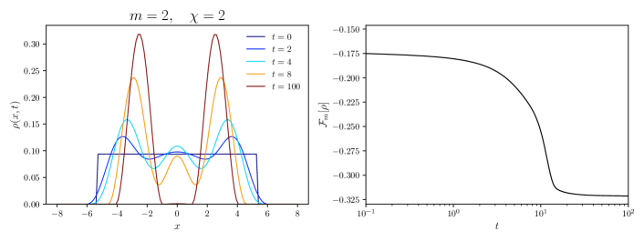
(a) Subcritical exponent $m<m_{c}$.

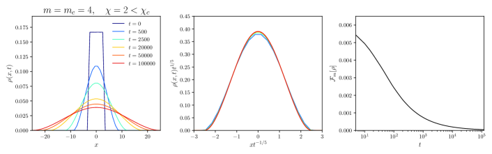
(b) Critical exponent $m=m_{c}$, subcritical mass $\chi<\chi_{c}$.

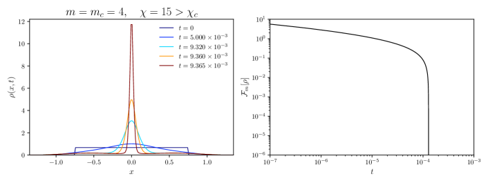
(c) Critical exponent $m=m_{c}$, supercritical mass $\chi>\chi_{c}$.

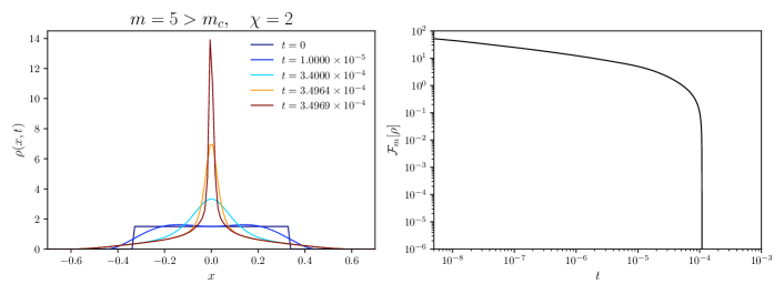
(d) Supercritical exponent $m>m_{c}$.

Figure 1. Numerical solutions to (1.1) in one spatial dimension for different values of $m$ and $\chi$, and decay of the free energy $\mathcal{F}_{m}[\rho]$ as a function of time.

A similar argument also works in the supercritical exponent case. If $m>m_{c}$ then

$$\frac{\mathrm{d}}{\mathrm{d}t}\mathrm{m}_{2}(\rho)\leq 2(d+2)\mathcal{F}_{m}[\rho]\leq 2(d+2)\mathcal{F}_{m}[\rho_{0}]<0\,,$$

for an initial datum with $\mathcal{F}_{m}[\rho_{0}]<0$, which can be chosen by Proposition 3.5. If the initial second moment is finite, then there exists some time $t^{*}>0$ such that $\mathrm{m}_{2}(\rho(t^{*}))=0$, implying that such solutions can only exist locally in time.

Our main results are also summarised in Figure 1, where we plot numerical solutions to (1.1) in one spatial dimension and for different values of the exponent $m$ and the mass parameter $\chi$. These are based on the finite-volume scheme presented in [2]. In particular, we observe that for subcritical exponent, solutions evolve towards a compactly supported steady state while the free energy stays bounded from below. For critical exponent with subcritical mass, we also notice that the free energy is bounded by zero from below, but in this case solutions tend to the self-similar profile mentioned in the previous sections. By plotting the solution in self-similar variables, this scaling is numerically verified. Finally, we observe finite-time blow-up for critical exponent with supercritical mass, and for supercritical exponent. In both cases, the free energy is unbounded from below.

4. Existence of weak solutions via the JKO scheme

Once we understood the properties of the free energy (1.5) we study existence of weak solutions of (1.1). The variational structure of Eq. (1.1) allows to construct a candidate approximate solutions by means of the so-called JKO scheme or minimising movement, cf. [43, 1]. For a fixed $\tau>0$, we define the following sequence recursively

$$\begin{split}\rho^{0}_{\tau}&:=\rho_{0},\\ \rho^{k+1}_{\tau}&\in\operatorname*{argmin}_{\rho\in\mathcal{P}(\mathbb{R}^{d})}\left\{\frac{\mathcal{W}_{2}^{2}(\rho,\rho^{k}_{\tau})}{2\tau}+\mathcal{F}_{m}[\rho]\right\},\,\mbox{given }\rho_{\tau}^{k},\;k\geq 0.\end{split}$$ (4.1)

First, we prove the above scheme is well-defined, which is not immediate due to the negative component in the energy functional, or destabilising term. Let us fix $\overline{\rho}\in\mathcal{P}_{2}^{a}(\mathbb{R}^{d})$ and define the functional

$$\begin{split}\mathcal{A}_{m}\colon&\mathcal{P}(\mathbb{R}^{d})\longrightarrow\overline{\mathbb{R}}\\ &\quad\rho\quad\mapsto\,\,\frac{\mathcal{W}_{2}^{2}(\rho,\overline{\rho})}{2\tau}+\mathcal{F}_{m}[\rho].\end{split}$$

Proposition 4.1.

Let $\overline{\rho}\in\mathcal{P}_{2}^{a}(\mathbb{R}^{d})$ and $1\leq m<2+\frac{2}{d}$ or $m=2+\frac{2}{d}$ with subcritical mass, i.e. $\chi<\chi_{c}$. The functional $\mathcal{A}_{m}$ admits minimisers in the set $\{\rho\in{\mathcal{P}}^{a}({\mathbb{R}^{d}}):\nabla\rho\in L^{2}({\mathbb{R}^{d}})\}$. Moreover, $\rho\in L^{p}({\mathbb{R}^{d}})$ for $p\in[1,2^{\ast}]$.

Existence of minimisers is based on the direct method of calculus of variations, as we prove below.

Remark 4.1.

Note that $\mathcal{W}^{2}_{2}(\rho,\overline{\rho})$ and $\|\nabla\rho\|^{2}_{L^{2}(\mathbb{R}^{d})}$ are lower semicontinuous with respect to weak convergence in $\mathcal{P}(\mathbb{R}^{d})$ and $L^{2}(\mathbb{R}^{d})$, respectively. However, the negative terms in the free energy,

$$-\frac{1}{m-1}\|\rho\|_{L^{m}(\mathbb{R}^{d})}^{m}\qquad\text{and}\qquad-\int_{{\mathbb{R}^{d}}}\rho\log\rho\,dx,$$

are both upper (and not lower) semicontinuous with respect to the weak convergence in $L^{m}(\mathbb{R}^{d})$. In particular, our functional $\mathcal{A}_{m}$ cannot be weakly lower semicontinuous.

Proof 4.1.

We split the proof into three parts.

Step 1: Boundedness from below and minimising sequence. Taking into account the definition of the free energy functional (1.5), we look for minimisers $\rho\in\mathcal{P}^{a}(\mathbb{R}^{d})$ such that $\nabla\rho\in L^{2}(\mathbb{R}^{d})$, otherwise the functional is infinite. Due to (3.1) we have the bound from below

$$\mathcal{F}_{m}[\rho]\geq C,$$ (4.2)

which implies $\mathcal{A}_{m}[\rho]\geq C$. Boundedness from below ensures we can consider a minimising sequence, $\rho_{n}$, for which we also know $\mathcal{A}_{m}\leq C$. Since the functional $\mathcal{F}_{m}$ is bounded from below, we obtain the bound for the second order moment

$$\begin{split}\mathrm{m}_{2}(\rho_{n})&\leq 2\mathcal{W}_{2}^{2}(\rho_{n},\overline{\rho})+2\mathrm{m}_{2}(\overline{\rho})=4\tau\mathcal{A}_{m}[\rho_{n}]-4\tau\mathcal{F}_{m}[\rho_{n}]+2\mathrm{m}_{2}(\overline{\rho})\\ &\leq CT\left(1+\mathrm{m}_{2}(\overline{\rho})\right),\end{split}$$ (4.3)

for a different constant $C$.

Step 2: Lower semicontinuity and compactness. First we comment on the lower semicontinuity of $\mathcal{A}_{m}$ with respect to a suitable convergence, i.e.

$$\liminf_{n\to\infty}\mathcal{A}_{m}[\rho_{n}]\geq\mathcal{A}_{m}[\rho].$$

From 4.1 we infer we cannot have lower semicontinuity with respect to weak convergence in all terms, but we have it with respect to the convergence

$$\nabla\rho_{n}\rightharpoonup\nabla\rho\quad\text{in }L^{2}(\mathbb{R}^{d}),$$

$$\begin{cases}\rho_{n}\rightarrow\rho\quad\text{in }L^{m}(\mathbb{R}^{d})&\text{if }1<m\leq 2+\frac{2}{d},\\ \rho_{n}\log\rho_{n}\rightarrow\rho\log\rho\quad\text{in }L^{1}(\mathbb{R}^{d})&\text{if }m=1.\end{cases}$$

Let us note that (3.2) combined with (4.2) implies that $\rho_{n}$ and $\nabla\rho_{n}$ are uniformly bounded on $L^{m}(\mathbb{R}^{d})$ and $L^{2}(\mathbb{R}^{d})$, respectively, as $\rho_{n}$ is a minimising sequence.

Step 2a: Strong $L^{m}$ convergence of $\rho_{n}$. If $1<m<2+\frac{2}{d}$ or $m=2+\frac{2}{d}$ with $\|\rho_{0}\|_{L^{1}(\mathbb{R}^{d})}<M_{c}$, since

$$\|\rho_{n}\|_{L^{m}(\mathbb{R}^{d})}\leq C,$$ (4.4)

by Banach-Alaoglu Theorem, up to pass to a subsequence,

$$\rho_{n}\rightharpoonup\rho\quad\text{weakly in }L^{m}(\mathbb{R}^{d}).$$ (4.5)

Taking into account (4.2), (4.3), and (4.4), we can restrict to the set

$$\mathcal{H}_{m}:=\left\{f\in\mathcal{P}^{a}(\mathbb{R}^{d}):\mathrm{m}_{2}(f),\,\|\nabla f\|_{L^{2}(\mathbb{R}^{d})},\,|\mathcal{F}_{m}[f]|\leq C\right\}.$$

Furthermore, from (3.3), if $f\in\mathcal{H}_{m}$, then

$$\|f\|_{L^{p}(\mathbb{R}^{d})}\leq C,$$ (4.6)

for all $p\in[1,2^{\ast}]$.

Next, we prove that $\mathcal{H}_{m}$ is relatively compact in $L^{m}(\mathbb{R}^{d})$ by means of Kolmogorov–Riesz–Fréchet Theorem [12, Corollary 4.27]. In particular, we first show the uniform continuity estimate: $\|f(\cdot+h)-f(\cdot)\|_{L^{m}(\mathbb{R}^{d})}\rightarrow 0$ as $|h|\rightarrow 0^{+}$. We distinguish two cases: $m=2$ and $m\neq 2$.

Case I: $m=2$. Let us take

$$\int_{\mathbb{R}^{d}}|f(x+h)-f(x)|^{2}\mathrm{d}x =\int_{\mathbb{R}^{d}}\left|\int_{0}^{1}\frac{\mathrm{d}}{\mathrm{d}s}\left(f(x+sh)\right)\,\mathrm{d}s\right|^{2}\,\mathrm{d}x$$

$$=|h|^{2}\int_{\mathbb{R}^{d}}\left|\int_{0}^{1}\nabla f(x+sh)\,\mathrm{d}s\right|^{2}\,\mathrm{d}x$$

$$\leq|h|^{2}\int_{\mathbb{R}^{d}}\int_{0}^{1}\left|\nabla f(x+sh)\right|^{2}\,\mathrm{d}s\,\mathrm{d}x\rightarrow 0,$$

since $\|\nabla f\|_{L^{2}(\mathbb{R}^{d})}\leq C$ for every $f\in\mathcal{H}_{m}$.

Case II: $m\neq 2$. We use $L^{p}$ interpolation and apply Case I afterwards. If $1<m<2$,

$$\|f(\cdot+h)-f(\cdot)\|_{L^{m}(\mathbb{R}^{d})} \leq\|f(\cdot+h)-f(\cdot)\|_{L^{1}(\mathbb{R}^{d})}^{\frac{2-m}{m}}\|f(\cdot+h)-f(\cdot)\|_{L^{2}(\mathbb{R}^{d})}^{\frac{2m-2}{m}}$$

$$\leq\left(2\|f\|_{L^{1}({\mathbb{R}^{d}})}\right)^{\frac{2-m}{m}}\|f(\cdot+h)-f(\cdot)\|_{L^{2}(\mathbb{R}^{d})}^{\frac{2m-2}{m}}\rightarrow 0.$$

If $2<m<2+\frac{2}{d}$ or $m=2+\frac{2}{d}$ with subcritical mass, by using a different $L^{p}$ interpolation we obtain

$$\|f(\cdot+h)-f(\cdot)\|_{L^{m}(\mathbb{R}^{d})} \leq\|f(\cdot+h)-f(\cdot)\|_{L^{2(m-1)}(\mathbb{R}^{d})}^{\frac{m-1}{m}}\|f(\cdot+h)-f(\cdot)\|_{L^{2}(\mathbb{R}^{d})}^{\frac{1}{m}}$$

$$\leq\left(2\|f\|_{L^{2(m-1)}(\mathbb{R}^{d})}\right)^{\frac{m-1}{m}}\|f(\cdot+h)-f(\cdot)\|_{L^{2}(\mathbb{R}^{d})}^{\frac{1}{m}}\rightarrow 0,$$

and the convergence follows from (3.3) given that $2(m-1)<2^{\ast}$.

In order to prove uniform integrability at infinity we first use Holder’s inequality to show that

$$\int_{\mathbb{R}^{d}\backslash B_{R}}f(x)^{m}\,\mathrm{d}x\leq\frac{1}{R^{2\delta}}\left(\int_{\mathbb{R}^{d}}|x|^{2}f(x)\,\mathrm{d}x\right)^{\delta}\left(\int_{\mathbb{R}^{d}}f(x)^{\frac{m-\delta}{1-\delta}}\,\mathrm{d}x\right)^{1-\delta}.$$

Now $\delta\in\left(0,1\right)$ can be chosen so that the exponent $p:=\frac{m-\delta}{1-\delta}$ satisfies $p\in[1,2^{\ast}]$. Hence, by (3.3), $\|f\|_{L^{p}(\mathbb{R}^{d})}$ is uniformly bounded. In particular, by taking the $R\rightarrow+\infty$ limit, and using that $f\in\mathcal{H}_{m}$ has uniformly bounded second moments we obtain the uniform integrability at infinity.

Then, $\mathcal{H}_{m}$ is relatively compact in $L^{m}(\mathbb{R}^{d})$ and combining it with (4.5) we obtain,

$$\rho_{n}\rightarrow\rho\quad\text{in }L^{m}(\mathbb{R}^{d}).$$ (4.7)

If $m=1$, since $\mathcal{F}_{1}[\rho]\geq\mathcal{F}_{2}[\rho]$ we have that $\mathcal{H}_{1}\subseteq\mathcal{H}_{2}$. From here, we recover (4.6), and (4.7) for $m=2$. We show $\rho_{n}\log\rho_{n}\to\rho\log\rho$ in $L^{1}({\mathbb{R}^{d}})$ via an extended version of Lebesgue’s Dominated Convergence Theorem [56, Chapter 4, Theorem 17]. Note that strong convergence in $L^{2}({\mathbb{R}^{d}})$ implies that, up to a subsequence,

$$\rho_{n}\log\rho_{n}\rightarrow\rho\log\rho\quad\text{a.e. in }x\in{\mathbb{R}^{d}}.$$

Furthermore, it is easy to check the majorant $|\rho_{n}(x)\log\rho_{n}(x)|\leq\rho_{n}^{2}(x)+\rho_{n}^{\frac{1}{2}}(x)$, for any $x\in{\mathbb{R}^{d}}$. We claim that $\rho_{n}^{2}+\rho_{n}^{\frac{1}{2}}\rightarrow\rho^{2}+\rho^{\frac{1}{2}}$ strongly in $L^{1}({\mathbb{R}^{d}})$. Since $\mathcal{H}_{1}\subseteq\mathcal{H}_{2}$ it is enough to show $\rho_{n}^{\frac{1}{2}}\rightarrow\rho^{\frac{1}{2}}$ strongly in $L^{1}({\mathbb{R}^{d}})$. Applying Jensen’s inequality for concave functions we have $\rho_{n}^{\frac{1}{2}}\in L^{1}({\mathbb{R}^{d}})$, while continuity of the square root function ensures

$$\rho_{n}^{\frac{1}{2}}(x)\rightarrow\rho^{\frac{1}{2}}(x)\quad\text{a.e. in }x\in{\mathbb{R}^{d}}.$$

By applying Fatou’s Lemma,

$$\liminf_{n\rightarrow\infty}\int_{{\mathbb{R}^{d}}}\rho_{n}^{\frac{1}{2}}\,dx\geq\int_{{\mathbb{R}^{d}}}\rho^{\frac{1}{2}}\,\mathrm{d}x\,,$$ (4.8)

and concavity implies,

$$\limsup_{n\rightarrow\infty}\int_{{\mathbb{R}^{d}}}\rho_{n}^{\frac{1}{2}}\,\mathrm{d}x\leq\int_{{\mathbb{R}^{d}}}\rho^{\frac{1}{2}}\,\mathrm{d}x.$$ (4.9)

Combining (4.8) and (4.9) we infer

$$\lim_{n\rightarrow\infty}\int_{{\mathbb{R}^{d}}}\rho_{n}^{\frac{1}{2}}\,dx=\int_{{\mathbb{R}^{d}}}\rho^{\frac{1}{2}}\,\mathrm{d}x.$$

Applying the extended Dominated Convergence Theorem we obtain

$$\rho_{n}\log\rho_{n}\rightarrow\rho\log\rho\quad\text{in }L^{1}({\mathbb{R}^{d}}).$$

Step 2b: Weak $L^{2}$ convergence of $\nabla\rho_{n}$. Given that $\nabla\rho$ is bounded in $L^{2}({\mathbb{R}^{d}})$, from Banach-Alaoglu Theorem we obtain that up to a subsequence,

$$\nabla\rho_{n}\rightharpoonup\nabla\rho\quad\text{weakly in }L^{2}(\mathbb{R}^{d}).$$

Note that the limit is $\nabla\rho$, which can be checked by testing $\nabla\rho$ against a smooth and compactly supported test function, and using the convergence $\rho_{n}\rightarrow\rho$ in $L^{m}(\mathbb{R}^{d})$ that we proved in the previous step.

Step 3: Existence of minimisers. Due to the Weierstrass criterion for the existence of minimisers, cf. e.g. [57, Box 1.1], $\mathcal{A}_{m}$ has at least one minimiser in $\mathcal{H}_{m}$. ∎

As mentioned in Section 3.1.1, the proof of Proposition 3.4 can be obtained by adapting the previous one to the functional $\mathcal{L}:{\mathcal{P}}^{a}({\mathbb{R}^{d}})\to\mathbb{R}$ given by

$$\mathcal{L}[u]=\mathcal{F}_{m_{c}}[u]+\frac{b}{2}\int|z|^{2}u(z)\,\mathrm{d}z.$$

Proof of Proposition 3.4.

Boundedness from below follows from Gagliardo–Nirenberg inequality and non-negativity of the additional term in $\mathcal{L}[u]$, as noted in 3.2. For a minimising sequence $\{u_{n}\}_{n\in\mathbb{N}}$, since $\chi<\chi_{c}$ we derive the following bounds, again as a consequence of Gagliardo–Nirenberg, cf. Proposition 3.2:

$$\|u_{n}\|_{L^{p}({\mathbb{R}^{d}})}\leq C,\quad\|\nabla u_{n}\|_{L^{2}({\mathbb{R}^{d}})}\leq C,\quad\mathrm{m}_{2}(u_{n})\leq C,$$

for $p\in[1,2^{*}]$ and a constant $C=C(m_{c},p,d,\chi)>0$. Kolmogorov–Riesz–Fréchet Theorem provides relatively compactness in $L^{m_{c}}({\mathbb{R}^{d}})$ for the set $\{f\in{\mathcal{P}}^{a}({\mathbb{R}^{d}}):\mathrm{m}_{2}(f),\|\nabla f\|_{L^{2}({\mathbb{R}^{d}})},|\mathcal{L}[\rho]|\leq C\}$, arguing as in 4.1. For the sake of completeness, we point out the additional term is lower semicontinuous with respect to the weak-$L^{2}$ convergence by applying a cut-off and monotone convergence Theorem — choosing $p=2$ we infer weak-$L^{2}$ convergence of $u_{n}$ from the above uniform bounds. Proceeding as in Proposition 4.1, and for $\chi<\chi_{c}$, we can show existence of minimisers in $\{u\in{\mathcal{P}}^{a}({\mathbb{R}^{d}}):\nabla u\in L^{2}({\mathbb{R}^{d}}),\mathrm{m}_{2}(u)<+\infty\}$. ∎

Proposition 4.1 guarantees the sequence is well-defined, as we can solve the minimisation problem in (4.1). Next, we set up the approximating solution to (1.1). Let $T>0$, and consider $N:=\left[\frac{T}{\tau}\right]$. We define the curve $\rho_{\tau}:[0,T]\rightarrow\mathcal{P}(\mathbb{R}^{d})$ as the piecewise constant interpolation

$$\rho_{\tau}(t):=\rho_{\tau}^{k},\quad t\in\left((k-1)\tau,k\tau\right],$$ (4.10)

where $\rho_{\tau}^{k}$ is defined in $\eqref{eq:JKO}$. We can prove convergence of this piecewise interpolation to a continuous curve with respect to the $2$-Wasserstein distance.

Lemma 4.1 (Narrow convergence & discrete uniform estimates).

Let $\rho_{0}\in\mathcal{P}_{2}^{a}({\mathbb{R}^{d}})$ such that $\mathcal{F}_{m}[\rho_{0}]<+\infty$ and $1\leq m<2+\frac{2}{d}$ or $m=2+\frac{2}{d}$ with subcritical mass $\chi<\chi_{c}$. There exists an absolutely continuous curve $\tilde{\rho}:[0,T]\rightarrow\mathcal{P}_{2}(\mathbb{R}^{d})$ such that, up to a subsequence, $\rho_{\tau}(t)$ narrowly converges to $\tilde{\rho}(t)$, uniformly in $t\in[0,T]$.

Moreover, we obtain the following discrete uniform bounds:

$$\sup_{k}\|\nabla\rho_{\tau}^{k}\|_{L^{2}({\mathbb{R}^{d}})} \leq C_{1}\left(\mathcal{F}_{m}[\rho_{0}]+\|\rho_{0}\|_{L^{1}({\mathbb{R}^{d}})}^{\alpha}\right)^{1/2}<+\infty;$$ (4.11)

$$\sup_{k}\|\rho_{\tau}^{k}\|_{L^{p}({\mathbb{R}^{d}})} \leq C_{2}<+\infty;$$ (4.12)

$$\mathrm{m}_{2}(\rho_{\tau}^{k}) \leq 2\mathrm{m}_{2}(\rho_{0})+4T\left(\mathcal{F}_{m}[\rho_{0}]+C\right),$$ (4.13)

for constants $C_{1}=C_{1}(m,d,\chi)>0$ and $C_{2}=C_{2}(m,p,d,\rho_{0},\chi)>0$, and for $p\in[1,2^{\ast}]$.

Proof.

By construction of the sequence we have

$$\mathcal{F}_{m}[\rho_{\tau}^{k}]\leq\frac{\mathcal{W}_{2}^{2}(\rho_{\tau}^{k},\rho_{\tau}^{k-1})}{2\tau}+\mathcal{F}_{m}[\rho_{\tau}^{k}]\leq\mathcal{F}_{m}[\rho_{\tau}^{k-1}].$$ (4.14)

In particular, this gives

$$\sup_{k}\mathcal{F}_{m}[\rho_{\tau}^{k}]\leq\mathcal{F}_{m}[\rho_{0}]<+\infty,$$

which together with (3.2) and (3.3) implies that $\|\nabla\rho_{\tau}^{k}\|_{L^{2}({\mathbb{R}^{d}})}$ and $\|\rho_{\tau}^{k}\|_{L^{p}({\mathbb{R}^{d}})}$ are uniformly bounded in $k$ and $\tau$ for $p\in[1,2^{\ast}]$. Hence we obtain (4.11) and (4.12).

Next, by summing up over $k$ in (4.14) and using that the free energy is bounded from below, (3.1), we deduce

$$\sum_{k=i+1}^{j}\frac{\mathcal{W}_{2}^{2}(\rho_{\tau}^{k},\rho_{\tau}^{k-1})}{2\tau}\leq\mathcal{F}_{m}[\rho_{\tau}^{i}]-\mathcal{F}_{m}[\rho_{\tau}^{j}]\leq\mathcal{F}_{m}[\rho_{0}]+C.$$ (4.15)

Therefore the $2$-Wasserstein distance between $\rho_{0}$ and $\rho_{\tau}(t)$ is uniformly bounded. Indeed, for $t\in((j-1)\tau,j\tau]$,

$$\mathcal{W}_{2}^{2}(\rho_{0},\rho_{\tau}(t)) \leq j\sum_{k=1}^{j}\mathcal{W}_{2}^{2}(\rho_{\tau}^{k},\rho_{\tau}^{k-1})\leq 2j\tau(\mathcal{F}_{m}[\rho_{0}]+C)\leq 2T(\mathcal{F}_{m}[\rho_{0}]+C).$$

Furthermore, we obtain second order moments are uniformly bounded on compact time intervals $[0,T]$ since

$$\mathrm{m}_{2}\left(\rho_{\tau}(t)\right)\leq 2\mathrm{m}_{2}(\rho_{0})+2\mathcal{W}_{2}^{2}(\rho_{0},\rho_{\tau}(t))\leq 2\mathrm{m}_{2}(\rho_{0})+4T\left(\mathcal{F}_{m}[\rho_{0}]+C\right).$$

Let us now prove equi-continuity. Consider $0\leq s<t$ such that $s\in((i-1)\tau,i\tau]$ and $t\in((j-1)\tau,j\tau]$. Using Cauchy–Schwarz inequality and (4.15) we have

$$\begin{split}\mathcal{W}_{2}(\rho_{\tau}(s),\rho_{\tau}(t))&\!\leq\!\sum_{k=i+1}^{j}\mathcal{W}_{2}(\rho_{\tau}^{k},\rho_{\tau}^{k-1})\!\leq\!\left(\sum_{k=i+1}^{j}\mathcal{W}_{2}^{2}(\rho_{\tau}^{k},\rho_{\tau}^{k-1})\right)^{\frac{1}{2}}\!\!|j-i|^{\frac{1}{2}}\\ &\!\leq\!\left(2(\mathcal{F}_{m}[\rho_{0}]+C)\right)^{\frac{1}{2}}\left(\sqrt{|t-s|}+\sqrt{\tau}\right).\end{split}$$ (4.16)

Thus, $\rho_{\tau}$ is $\frac{1}{2}$-Hölder equi-continuous up to a negligible error of order $\sqrt{\tau}$. Therefore, by a refined version of the Ascoli-Arzelà Theorem [1, Proposition 3.3.1], we obtain that $\rho_{\tau}$ admits a subsequence narrowly converging to a limit $\tilde{\rho}$ as $\tau\rightarrow 0^{+}$, uniformly on $[0,T]$. Moreover, using the uniform bound (4.13) and that $|\cdot|^{2}$ is lower semicontinuous and bounded from below, we obtain that the limiting curve $\tilde{\rho}$ has bounded second order moments,

$$\mathrm{m}_{2}(\tilde{\rho}(t))\leq\liminf_{\tau\downarrow 0}\mathrm{m}_{2}(\rho_{\tau}(t)),\quad\forall t\in[0,T].\qed$$

The bounds (4.12) and (4.11) imply weak convergence of the interpolation $\rho_{\tau}$ to a probability density $\tilde{\rho}$ with regularity provided below.

Proposition 4.2 (Weak convergence).

Let $\rho_{0}\in\mathcal{P}_{2}^{a}({\mathbb{R}^{d}})$ such that $\mathcal{F}_{m}[\rho_{0}]<+\infty$ and $1\leq m<2+\frac{2}{d}$ or $m=2+\frac{2}{d}$ with subcritical mass $\chi<\chi_{c}$. The piecewise interpolation $\rho_{\tau}$ in (4.10) is such that $\rho_{\tau}\in L^{\infty}([0,T];L^{p}({\mathbb{R}^{d}}))\cap L^{\infty}([0,T];H^{1}({\mathbb{R}^{d}}))$, for any $p\in[1,2^{\ast}]$. In particular, the limit $\tilde{\rho}$ belongs to $L^{\infty}([0,T];L^{p}({\mathbb{R}^{d}}))\cap L^{\infty}([0,T];H^{1}({\mathbb{R}^{d}}))$ and

$$\rho_{\tau}\rightharpoonup\tilde{\rho}\quad\mbox{in }L^{2}([0,T];H^{1}({\mathbb{R}^{d}})).$$

Proof.

From (4.12) in 4.1 we have

$$\|\rho_{\tau}\|_{L^{\infty}([0,T];L^{p}({\mathbb{R}^{d}}))}=\sup_{t\in(0,T)}\|\rho_{\tau}(t)\|_{L^{p}({\mathbb{R}^{d}})}=\sup_{k}\|\rho_{\tau}^{k}\|_{L^{p}({\mathbb{R}^{d}})}<+\infty,$$

for $p\in[1,2^{\ast}]$. Analogously, from (4.11) we obtain $\nabla\rho_{\tau}\in L^{\infty}([0,T];L^{2}({\mathbb{R}^{d}}))$. In particular, for any compact time interval $[0,T]$ with $T>0$, we have $\|\rho_{\tau}\|_{L^{2}([0,T];H^{1}({\mathbb{R}^{d}}))}\leq C$ uniformly in $\tau$ and the weak convergence follows from Banach-Alaoglu Theorem. Regularity of the limit follows from standard arguments. ∎

The uniform-in-$\tau$ $L^{\infty}([0,T];H^{1}({\mathbb{R}^{d}}))$ estimate allows us to obtain strong convergence of $\rho_{\tau}$ via a refined version of the Aubin-Lions Lemma due to Rossi and Savaré — cf. 2.1.

Proposition 4.3 (Strong convergence of $\rho_{\tau}$).

Let $\rho_{0}\in\mathcal{P}_{2}^{a}({\mathbb{R}^{d}})$ such that $\mathcal{F}_{m}[\rho_{0}]<+\infty$ and $1\leq m<2+\frac{2}{d}$ or $m=2+\frac{2}{d}$ with subcritical mass $\chi<\chi_{c}$. The sequence $\rho_{\tau}$ converges, up to a subsequence, strongly to the curve $\tilde{\rho}$ in $L^{2}([0,T];L^{2}({\mathbb{R}^{d}}))$ for every $T>0$.

Proof.

We apply 2.1 to a subset $U=\{\rho_{\tau}\}_{\tau\geq 0}$ for $X=L^{2}({\mathbb{R}^{d}})$ and $g:=\mathcal{W}_{2}$, the 2-Wasserstein distance. Further, we consider the functional $\mathcal{I}:L^{2}({\mathbb{R}^{d}})\rightarrow[0,+\infty]$ defined by

$$\mathcal{I}[\rho]=\begin{cases}\|\rho\|_{H^{1}({\mathbb{R}^{d}})}^{2}+\int_{\mathbb{R}^{d}}|x|^{2}\rho(x)\,\mathrm{d}x&\rho\in\mathcal{P}_{2}(\mathbb{R}^{d})\cap H^{1}({\mathbb{R}^{d}}),\\ +\infty&\mbox{otherwise}.\end{cases}$$

Note that $\mathcal{W}_{2}$ is a distance on the proper domain of $\mathcal{I}$. Indeed, if $\mathcal{I}[\rho]<\infty$ then $\rho\in\mathcal{P}_{2}(\mathbb{R}^{d})$. Lower semicontinuity of $\mathcal{I}$ follows from standard arguments — see for instance [14].

Next, let $B_{c}=\{\rho\in L^{2}({\mathbb{R}^{d}}):\mathcal{I}[\rho]\leq c\}$ be a sublevel of $\mathcal{I}$. We notice that $B_{c}\subset\mathcal{P}_{2}({\mathbb{R}^{d}})\cap H^{1}({\mathbb{R}^{d}})$ and thus we can apply Kolmogorov-Riesz-Fréchet Theorem [12, Corollary 4.27] as in the proof of 4.1 to obtain that $B_{c}$ is relatively compact. Hence we have $\mathcal{I}$ is an admissible functional.

The tightness condition (2.1) follows from the uniform-in-$\tau$ second order moment and $L^{\infty}([0,T];H^{1}({\mathbb{R}^{d}}))$ bounds for $\rho_{\tau}$ given in (4.13) and 4.2. The integral equi-continuity condition (2.2) can be seen from the Hölder equi-continuity of $\rho_{\tau}$, proved in 4.1. More precisely, for $h>\tau$ we have

$$\int_{0}^{T-h}\mathcal{W}_{2}\left(\rho_{\tau}(t+h),\rho_{\tau}(t)\right)\mathrm{d}t\leq\int_{0}^{T-h}C\left(\sqrt{h}+\sqrt{\tau}\right)\mathrm{d}t\leq 2CT\sqrt{h},$$

for a constant $C>0$ independent of $\tau$ and $h$. If instead, $h<\tau$, we can write

$$\int_{0}^{T-h}\mathcal{W}_{2}\left(\rho_{\tau}(t+h),\rho_{\tau}(t)\right)\mathrm{d}t \leq h\sum_{k=0}^{N-1}\mathcal{W}_{2}(\rho_{\tau}^{k+1},\rho_{\tau}^{k})$$

$$\leq h\sqrt{N}\sum_{k=0}^{N-1}\mathcal{W}_{2}^{2}(\rho_{\tau}^{k+1},\rho_{\tau}^{k})\leq Ch\sqrt{T},$$

where $C>0$ is the constant defined in (4.15).

Hence we can apply 2.1 to obtain that there exists a subsequence, that we label by $\tau\downarrow 0$, such that $\rho_{\tau}$ converges in measure to $\tilde{\rho}$, as in (2.3), where $X:=L^{2}({\mathbb{R}^{d}})$. Let us denote by $A_{\delta}(\tau):=\{t\in(0,T):\;\|\rho_{\tau}(t)-\tilde{\rho}(t)\|_{X}\geq\delta\}$, which vanishes as $\tau\to 0$. Owing to (4.12) and Proposition 4.2 we can prove (see e.g. [22, Proposition 4.3])

$$\limsup_{\tau\to 0}\|\rho_{\tau}-\tilde{\rho}\|^{2}_{L^{2}([0,T];L^{2}({\mathbb{R}^{d}}))}\leq\delta T^{1/2},$$

hence strong convergence in $L^{2}([0,T];L^{2}({\mathbb{R}^{d}}))$ since $\delta$ is arbitrarily small. ∎

4.1. Flow interchange

The strong convergence of the sequence $\rho_{\tau}$ obtained in 4.3 is not enough to pass to the limit in the Euler-Lagrange equation associated to (4.1) and arrive to a weak formulation of our equation. We use the heat equation as auxiliary flow to obtain uniform bounds on the Hessian of the sequence $\{\rho_{\tau}\}_{\tau}$, cf. section 2. More precisely, we exploit that the heat equation is a $2$-Wasserstein gradient flow of the entropy functional $\mathcal{E}[\rho]=\int\rho\log\rho\,\mathrm{d}x$.

In the following, for $\mu\in\mathcal{P}_{2}({\mathbb{R}^{d}})$ such that $\mathcal{E}[\mu]<\infty$, we denote by $S_{\mathcal{E}}^{t}\mu$ the solution at time $t$ of the heat equation for an initial value $\mu$ at $t=0$. Furthermore, we also define the dissipation of $\mathcal{F}_{m}$ along $S_{\mathcal{E}}$ by

$$D_{\mathcal{E}}\mathcal{F}_{m}[\rho]:=\limsup_{s\downarrow 0}\left\{\frac{\mathcal{F}_{m}[\rho]-\mathcal{F}_{m}[S_{\mathcal{E}}^{s}\rho]}{s}\right\}.$$

Remark 4.2.

Given some initial datum $\mu_{0}\in\mathcal{P}({\mathbb{R}^{d}})$ the solution of the heat equation, $S_{\mathcal{E}}^{t}\mu_{0}$, can be written as the convolution of the heat kernel $G_{t}$ with the initial condition, i.e.

$$S_{\mathcal{E}}^{t}\mu_{0}=G_{t}*\mu_{0}={\left(4\pi t\right)^{-d/2}}\int_{\mathbb{R}^{d}}e^{-{|x-y|^{2}}/{4t}}\mathrm{d}\mu_{0}(y).$$

As a consequence, $S_{\mathcal{E}}^{t}\mu_{0}\in C^{\infty}\left((0,+\infty)\times{\mathbb{R}^{d}}\right)$. Moreover, for solutions of the heat equation we can integrate by parts to obtain the well-known equality

$$\int_{\mathbb{R}^{d}}|\Delta S_{\mathcal{E}}^{t}\mu_{0}|^{2}\,\mathrm{d}x=\int_{\mathbb{R}^{d}}|D^{2}S_{\mathcal{E}}^{t}\mu_{0}|^{2}\,\mathrm{d}x\,.$$ (4.17)

We are now ready to prove an $H^{2}$ bound for $\rho^{\tau}$.

Lemma 4.2 ($H^{2}$ uniform bound).

Let $\rho_{0}$ such that $\mathcal{F}_{m}[\rho_{0}]<+\infty$, and $1\leq m<2+\frac{2}{d}$ or $m=2+\frac{2}{d}$ with subcritical mass $\chi<\chi_{c}$. The piecewise interpolation $\rho_{\tau}$ constructed in (4.10) is such that $\rho_{\tau}\in L^{2}([0,T];H^{2}({\mathbb{R}^{d}}))$. In particular, we obtain the uniform-in-$\tau$ bound

$$\|\Delta\rho_{\tau}\|_{L^{2}([0,T];L^{2}({\mathbb{R}^{d}}))}^{2}\leq d\|D^{2}\rho_{\tau}\|_{L^{2}([0,T];L^{2}({\mathbb{R}^{d}}))}^{2}\leq C,$$

where $C=C(m,d,\rho_{0},T)>0$.

Proof.

For all $s>0$, we consider $S_{\mathcal{E}}^{s}\rho_{\tau}^{k+1}$. Then, by the definition of the scheme (4.1) and of $\rho_{\tau}^{k+1}$, we have the inequality

$$\frac{1}{2\tau}\mathcal{W}_{2}^{2}(\rho_{\tau}^{k},\rho_{\tau}^{k+1})+\mathcal{F}_{m}[\rho_{\tau}^{k+1}]\leq\frac{1}{2\tau}\mathcal{W}_{2}^{2}(\rho_{\tau}^{k},S_{\mathcal{E}}^{s}\rho_{\tau}^{k+1})+\mathcal{F}_{m}[S_{\mathcal{E}}^{s}\rho_{\tau}^{k+1}],$$

from which we obtain,

$$\tau\frac{\mathcal{F}_{m}[\rho_{\tau}^{k+1}]-\mathcal{F}_{m}[S_{\mathcal{E}}^{s}\rho_{\tau}^{k+1}]}{s}\leq\frac{1}{2}\frac{\mathcal{W}_{2}^{2}(\rho_{\tau}^{k},S_{\mathcal{E}}^{s}\rho_{\tau}^{k+1})-\mathcal{W}_{2}^{2}(\rho_{\tau}^{k},\rho_{\tau}^{k+1})}{s}.$$

By taking the $\limsup$ as $s\downarrow 0$ we obtain

$$\tau D_{\mathcal{E}}\mathcal{F}_{m}[\rho_{\tau}^{k+1}]\leq\frac{1}{2}\left.\frac{\mathrm{d}^{+}}{\mathrm{d}t}\right|_{t=0}\mathcal{W}_{2}^{2}(\rho_{\tau}^{k},S_{\mathcal{E}}^{t}\rho_{\tau}^{k+1})\leq\mathcal{E}[\rho_{\tau}^{k}]-\mathcal{E}[\rho_{\tau}^{k+1}],$$ (4.18)

where in the last inequality we use the (EVI), as $S_{\mathcal{E}}$ is a $0$-flow, cf. Definition 2.4. Note that

$$\begin{split}D_{\mathcal{E}}\mathcal{F}_{m}[\rho_{\tau}^{k+1}]&=\limsup_{s\downarrow 0}\left\{\frac{\mathcal{F}_{m}[\rho_{\tau}^{k+1}]-\mathcal{F}_{m}[S_{\mathcal{E}}^{s}\rho_{\tau}^{k+1}]}{s}\right\}\\ &=\limsup_{s\downarrow 0}\int_{0}^{1}\left(-\left.\frac{\mathrm{d}}{\mathrm{d}z}\right|_{z=st}\mathcal{F}_{m}[S_{\mathcal{E}}^{z}\rho_{\tau}^{k+1}]\right)\,\mathrm{d}t.\end{split}$$ (4.19)

From this point of the proof, we distinguish between two cases.

Case I: $1<m<2+\frac{2}{d}$ or $m=2+\frac{2}{d}$ with subcritical mass $\chi<\chi_{c}$. Let us compute the time derivative:

$$\begin{split}\frac{\mathrm{d}}{\mathrm{d}t}\mathcal{F}_{m}[S_{\mathcal{E}}^{t}\rho_{\tau}^{k+1}]=&-\int_{{\mathbb{R}^{d}}}|\Delta S_{\mathcal{E}}^{t}\rho_{\tau}^{k+1}|^{2}\mathrm{d}x\\ &-\frac{\chi m}{m-1}\int_{{\mathbb{R}^{d}}}(S_{\mathcal{E}}^{t}\rho_{\tau}^{k+1})^{m-1}\Delta S_{\mathcal{E}}^{t}\rho_{\tau}^{k+1}\mathrm{d}x.\end{split}$$ (4.20)

Therefore, combining (4.18), (4.19) and (4.20) we obtain

$$\tau\limsup_{s\downarrow 0}\int_{0}^{1}\left(\int_{{\mathbb{R}^{d}}}|\Delta S_{\mathcal{E}}^{st}\rho_{\tau}^{k+1}|^{2}\,\mathrm{d}x+\frac{\chi m}{m-1}\int_{{\mathbb{R}^{d}}}(S_{\mathcal{E}}^{st}\rho_{\tau}^{k+1})^{m-1}\Delta S_{\mathcal{E}}^{st}\rho_{\tau}^{k+1}\,\mathrm{d}x\right)\,\mathrm{d}t$$

$$\qquad\leq\mathcal{E}[\rho_{\tau}^{k}]-\mathcal{E}[\rho_{\tau}^{k+1}].$$

By applying Young’s inequality we have

$$\int_{{\mathbb{R}^{d}}}|\Delta S_{\mathcal{E}}^{st}\rho_{\tau}^{k+1}|^{2}\,\mathrm{d}x+\frac{\chi m}{m-1}\int_{{\mathbb{R}^{d}}}(S_{\mathcal{E}}^{st}\rho_{\tau}^{k+1})^{m-1}\Delta S_{\mathcal{E}}^{st}\rho_{\tau}^{k+1}\,\mathrm{d}x$$

$$\qquad\geq\int_{{\mathbb{R}^{d}}}|\Delta S_{\mathcal{E}}^{st}\rho_{\tau}^{k+1}|^{2}\,\mathrm{d}x-\frac{\chi m}{m-1}\int_{{\mathbb{R}^{d}}}|(S_{\mathcal{E}}^{st}\rho_{\tau}^{k+1})^{m-1}||\Delta S_{\mathcal{E}}^{st}\rho_{\tau}^{k+1}|\,\mathrm{d}x$$

$$\qquad\geq\frac{1}{2}\int_{{\mathbb{R}^{d}}}|\Delta S_{\mathcal{E}}^{st}\rho_{\tau}^{k+1}|^{2}\,\mathrm{d}x-\frac{\chi^{2}m^{2}}{2(m-1)^{2}}\int_{{\mathbb{R}^{d}}}|S_{\mathcal{E}}^{st}\rho_{\tau}^{k+1}|^{2(m-1)}\,\mathrm{d}x\,,$$

which gives

$$\frac{\tau}{2}\liminf_{s\downarrow 0}\int_{0}^{1}\int_{{\mathbb{R}^{d}}}|\Delta S_{\mathcal{E}}^{st}\rho_{\tau}^{k+1}|^{2}\,\mathrm{d}x\,\mathrm{d}t$$

$$\qquad\leq\mathcal{E}[\rho_{\tau}^{k}]-\mathcal{E}[\rho_{\tau}^{k+1}]+\tau\frac{\chi^{2}m^{2}}{2(m-1)^{2}}\limsup_{s\downarrow 0}\int_{0}^{1}\int_{{\mathbb{R}^{d}}}|S_{\mathcal{E}}^{st}\rho_{\tau}^{k+1}|^{2(m-1)}\,\mathrm{d}x\,\mathrm{d}t.$$

In order to take the $s\downarrow 0$ limit in the above expression, first we note that, in view of 4.2, we can write $\|\Delta S_{\mathcal{E}}^{st}\rho_{\tau}^{k+1}\|_{L^{2}({\mathbb{R}^{d}})}=\|D^{2}S_{\mathcal{E}}^{st}\rho_{\tau}^{k+1}\|_{L^{2}({\mathbb{R}^{d}})}$. Since the auxiliary flow is the heat equation with initial datum $\rho_{\tau}^{k+1}\in H^{1}({\mathbb{R}^{d}})$, we have $S_{\mathcal{E}}^{t}\rho_{\tau}^{k+1}\to\rho_{\tau}^{k+1}$ in $L^{2}({\mathbb{R}^{d}})$ as well as $\nabla S_{\mathcal{E}}^{t}\rho_{\tau}^{k+1}\to\nabla\rho_{\tau}^{k+1}$ in $L^{2}({\mathbb{R}^{d}})$ as $t\downarrow 0$ — by noticing that $\nabla S_{\mathcal{E}}^{t}\rho_{\tau}^{k+1}$ is a solution to the heat equation with initial datum $\nabla\rho_{\tau}^{k+1}\in L^{2}({\mathbb{R}^{d}})$. By the weak lower-semicontinuity of the $H^{1}$ seminorm we have

$$\liminf_{s\downarrow 0}\int_{0}^{1}\int_{{\mathbb{R}^{d}}}|D^{2}S_{\mathcal{E}}^{st}\rho_{\tau}^{k+1}|^{2}\,\mathrm{d}x\,\mathrm{d}t\geq\int_{{\mathbb{R}^{d}}}|D^{2}\rho_{\tau}^{k+1}|^{2}\,\mathrm{d}x\,.$$ (4.21)

Next, we focus on the term involving $\|S_{\mathcal{E}}^{st}\rho_{\tau}^{k+1}\|_{L^{2(m-1)}({\mathbb{R}^{d}})}$ and distinguish between two cases, depending on the value of $m$. We apply Young’s convolution inequality to $S_{\mathcal{E}}^{st}\rho_{\tau}^{k+1}=G_{st}*\rho_{\tau}^{k+1}$, as noticed in 4.2.

If $\frac{3}{2}\leq m<2+\frac{2}{d}$ or $m=2+\frac{2}{d}$ with subcritical mass, then $1\leq 2(m-1)<2^{\ast}$ and, by (3.3), $\rho_{\tau}^{k+1}\in L^{2(m-1)}({\mathbb{R}^{d}})$. Furthermore, we have

$$\|S_{\mathcal{E}}^{st}\rho_{\tau}^{k+1}\|_{L^{2(m-1)}({\mathbb{R}^{d}})}\leq\|G_{st}\|_{L^{1}({\mathbb{R}^{d}})}\|\rho_{\tau}^{k+1}\|_{L^{2(m-1)}({\mathbb{R}^{d}})}=\|\rho_{\tau}^{k+1}\|_{L^{2(m-1)}({\mathbb{R}^{d}})},$$

In particular, we obtain

$$\limsup_{s\downarrow 0}\int_{0}^{1}\int_{{\mathbb{R}^{d}}}|S_{\mathcal{E}}^{st}\rho_{\tau}^{k+1}|^{2(m-1)}\,\mathrm{d}x\,\mathrm{d}t\leq\int_{{\mathbb{R}^{d}}}|\rho_{\tau}^{k+1}|^{2(m-1)}\,\mathrm{d}x\,.$$

If $1<m<\frac{3}{2}$, we use that the function $|\cdot|^{2(m-1)}$ is concave and apply Jensen’s inequality to find

$$\int_{{\mathbb{R}^{d}}}|S_{\mathcal{E}}^{st}\rho_{\tau}^{k+1}|^{2(m-1)}\,\mathrm{d}x \leq\left|\int_{{\mathbb{R}^{d}}}S_{\mathcal{E}}^{st}\rho_{\tau}^{k+1}\,\mathrm{d}x\right|^{2(m-1)}=\|G_{st}*\rho_{\tau}^{k+1}\|_{L^{1}({\mathbb{R}^{d}})}^{2(m-1)}$$

$$\leq\|G_{st}\|_{L^{1}({\mathbb{R}^{d}})}^{2(m-1)}\|\rho_{\tau}^{k+1}\|_{L^{1}({\mathbb{R}^{d}})}^{2(m-1)}=\|\rho_{\tau}^{k+1}\|_{L^{1}({\mathbb{R}^{d}})}^{2(m-1)},$$

whence

$$\limsup_{s\downarrow 0}\int_{0}^{1}\int_{{\mathbb{R}^{d}}}|S_{\mathcal{E}}^{st}\rho_{\tau}^{k+1}|^{2(m-1)}\,\mathrm{d}x\,\mathrm{d}t\leq\left|\int_{{\mathbb{R}^{d}}}\rho_{\tau}^{k+1}\,\mathrm{d}x\,\right|^{2(m-1)}.$$

As a consequence,

$$\frac{\tau}{2}\int_{{\mathbb{R}^{d}}}|D^{2}\rho_{\tau}^{k+1}|^{2}\,\mathrm{d}x\leq\mathcal{E}[\rho_{\tau}^{k}]-\mathcal{E}[\rho_{\tau}^{k+1}]+\tau\frac{\chi^{2}m^{2}}{2(m-1)^{2}}\|\rho_{\tau}^{k+1}\|_{L^{q}({\mathbb{R}^{d}})}^{2(m-1)},$$

with $q=2(m-1)$ for $\frac{3}{2}\leq m<2+\frac{2}{d}$ or $m=2+\frac{2}{d}$ with subcritical mass, and $q=1$ for $1<m<\frac{3}{2}$. By summing up over $k$ from $0$ to $N-1$, considering that $x\log x\leq x^{2}$ and 2.1, we recover, further using Jensen’s inequality for concave functions for $q=1$,

$$\frac{1}{2}\|D^{2}\rho_{\tau}\|^{2}_{L^{2}([0,T];L^{2}({\mathbb{R}^{d}}))} \leq\mathcal{E}[\rho_{0}]-\mathcal{E}[\rho_{\tau}^{N}]+\frac{\chi^{2}m^{2}}{2(m-1)^{2}}\sum_{k=0}^{N-1}\tau\|\rho_{\tau}^{k+1}\|_{L^{q}({\mathbb{R}^{d}})}^{2(m-1)}$$

$$\leq\|\rho_{0}\|_{L^{2}({\mathbb{R}^{d}})}^{2}+C(1+\mathrm{m}_{2}(\rho_{\tau}^{N}))$$

$$\quad+\frac{\chi^{2}m^{2}}{2(m-1)^{2}T^{2(m-1)-1}}\|\rho_{\tau}\|_{L^{q}([0,T];L^{q}({\mathbb{R}^{d}}))}^{2(m-1)},$$

which is uniformly bounded, due to 4.1. In particular, we also obtain

$$\|\Delta\rho_{\tau}\|_{L^{2}([0,T];L^{2}({\mathbb{R}^{d}}))}\leq\sqrt{d}\|D^{2}\rho_{\tau}\|_{L^{2}([0,T];L^{2}({\mathbb{R}^{d}}))}\leq C(m,d,\rho_{0},\chi,T).$$

Case II: $m=1$. Let us compute the time derivative,

$$\begin{split}\frac{\mathrm{d}}{\mathrm{d}t}\mathcal{F}_{1}[S_{\mathcal{E}}^{t}\rho_{\tau}^{k+1}]&=-\int_{{\mathbb{R}^{d}}}|\Delta S_{\mathcal{E}}^{t}\rho_{\tau}^{k+1}|^{2}\,\mathrm{d}x\\ &\quad-\chi\int_{{\mathbb{R}^{d}}}\Delta S_{\mathcal{E}}^{t}\rho_{\tau}^{k+1}(1+\log S_{\mathcal{E}}^{t}\rho_{\tau}^{k+1})\,\mathrm{d}x\\ &=-\int_{{\mathbb{R}^{d}}}|\Delta S_{\mathcal{E}}^{t}\rho_{\tau}^{k+1}|^{2}\,\mathrm{d}x\\ &\quad+\chi\int_{{\mathbb{R}^{d}}}\nabla S_{\mathcal{E}}^{t}\rho_{\tau}^{k+1}\cdot\nabla\log S_{\mathcal{E}}^{t}\rho_{\tau}^{k+1}\,\mathrm{d}x\,.\end{split}$$ (4.22)

By combining (4.18), (4.19) and (4.22), we obtain

$$\tau\limsup_{s\downarrow 0}\int_{0}^{1}\left(\int_{{\mathbb{R}^{d}}}|\Delta S_{\mathcal{E}}^{st}\rho_{\tau}^{k+1}|^{2}\,\mathrm{d}x-\chi\int_{{\mathbb{R}^{d}}}\nabla S_{\mathcal{E}}^{st}\rho_{\tau}^{k+1}\cdot\nabla\log S_{\mathcal{E}}^{st}\rho_{\tau}^{k+1}\,\mathrm{d}x\right)\,\mathrm{d}t$$

$$\qquad\leq\mathcal{E}[\rho_{\tau}^{k}]-\mathcal{E}[\rho_{\tau}^{k+1}]\,.$$

Similarly to the previous case, we obtain

$$\tau\liminf_{s\downarrow 0}\int_{0}^{1}\int_{{\mathbb{R}^{d}}}|\Delta S_{\mathcal{E}}^{st}\rho_{\tau}^{k+1}|^{2}\,\mathrm{d}x\,\mathrm{d}t$$

$$\qquad\leq\mathcal{E}[\rho_{\tau}^{k}]-\mathcal{E}[\rho_{\tau}^{k+1}]+\chi\tau\limsup_{s\downarrow 0}\int_{0}^{1}\int_{{\mathbb{R}^{d}}}\nabla S_{\mathcal{E}}^{st}\rho_{\tau}^{k+1}\cdot\nabla\log S_{\mathcal{E}}^{st}\rho_{\tau}^{k+1}\,\mathrm{d}x\,\mathrm{d}t$$

$$\qquad=\mathcal{E}[\rho_{\tau}^{k}]-\mathcal{E}[\rho_{\tau}^{k+1}]+\chi\tau\limsup_{s\downarrow 0}\left(\mathcal{E}[\rho_{\tau}^{k+1}]-\mathcal{E}[S_{\mathcal{E}}^{s}\rho_{\tau}^{k+1}]\right),$$

where we recognised the third term as the Fisher information functional for solutions of the heat equation. Next, using well-known properties of the heat equation and the estimates in Lemma 4.1 we have

$$\limsup_{s\downarrow 0}\left(\mathcal{E}[\rho_{\tau}^{k+1}]-\mathcal{E}[S_{\mathcal{E}}^{s}\rho_{\tau}^{k+1}]\right)\leq C,$$

for a constant $C$ independent of $k$. By summing up over $k$ from $0$ to $N-1$, and using (4.17) and (4.21) again we obtain

$$\|D^{2}\rho_{\tau}\|_{L^{2}([0,T];L^{2}({\mathbb{R}^{d}}))}^{2}\leq\mathcal{E}[\rho_{0}]-\mathcal{E}[\rho_{\tau}^{N}]+\tau NC,$$

and in particular, $\Delta\rho_{\tau}$ is uniformly bounded in $L^{2}([0,T];L^{2}({\mathbb{R}^{d}}))$. ∎

Proposition 4.4 (Strong convergence of $\nabla\rho_{\tau}$).

Let $\rho_{0}$ such that $\mathcal{F}_{m}[\rho_{0}]<+\infty$, and $1\leq m<2+\frac{2}{d}$ or $m=2+\frac{2}{d}$ with subcritical mass $\chi<\chi_{c}$. Up to a subsequence, the sequence $\rho_{\tau}:[0,T]\rightarrow\mathcal{P}_{2}({\mathbb{R}^{d}})$ converges strongly to the curve $\tilde{\rho}$ in $L^{2}([0,T];H^{1}({\mathbb{R}^{d}}))$.

Proof.

First note that due to 4.2, $D^{2}\rho_{\tau}\rightharpoonup D^{2}\tilde{\rho}$ in $L^{2}([0,T];L^{2}({\mathbb{R}^{d}}))$. The limit can be uniquely identified by integrating against a smooth and compactly supported test function and using the convergence $\nabla\rho_{\tau}\rightharpoonup\nabla\tilde{\rho}$ in $L^{2}([0,T];L^{2}({\mathbb{R}^{d}}))$, cf. 4.2. Next, we claim strong convergence of $\rho_{\tau}$ in $L^{2}([0,T];H^{1}({\mathbb{R}^{d}}))$ follows from the strong convergence in $L^{2}([0,T];L^{2}({\mathbb{R}^{d}}))$, cf. 4.3, and the fact that $\|\rho_{\tau}\|_{L^{2}([0,T];H^{2}({\mathbb{R}^{d}}))}$ is uniformly bounded in $\tau$, as given in 4.2. More precisely, using Gagliardo–Nirenberg (for the gradient) and Cauchy–Schwarz inequalities, we obtain

$$\int_{0}^{T} \|\nabla\rho_{\tau}(t)-\nabla\tilde{\rho}(t)\|^{2}_{L^{2}({\mathbb{R}^{d}})}\,\mathrm{d}t$$

$$\leq C\int_{0}^{T}\|D^{2}\rho_{\tau}(t)-D^{2}\tilde{\rho}(t)\|_{L^{2}({\mathbb{R}^{d}})}\|\rho_{\tau}(t)-\tilde{\rho}(t)\|_{L^{2}({\mathbb{R}^{d}})}\,\mathrm{d}t$$

$$\leq C\|D^{2}\rho_{\tau}-D^{2}\tilde{\rho}\|_{L^{2}([0,T];L^{2}({\mathbb{R}^{d}}))}\|\rho_{\tau}-\tilde{\rho}\|_{L^{2}([0,T];L^{2}({\mathbb{R}^{d}}))}.$$

The result is obtained by using that the norms $\|D^{2}\rho_{\tau}\|_{L^{2}([0,T];L^{2}({\mathbb{R}^{d}}))}$ and $\|D^{2}\tilde{\rho}\|_{L^{2}([0,T];L^{2}({\mathbb{R}^{d}}))}$ are uniformly bounded in $\tau$ — 4.2. ∎

The strong convergence of $\nabla\rho_{\tau}$ allows us to improve the result of $\rho_{\tau}$ given by Proposition 4.3 via interpolation inequalities. In particular, we obtain the integrability exponent needed to pass to the limit $\tau\rightarrow 0$ in the weak formulation.

Corollary 4.1 (Higher integrability).

Assume $1<m<2+\frac{2}{d}$ or $m=2+\frac{2}{d}$ with subcritical mass $\chi<\chi_{c}$. Then, the sequence $\rho_{\tau}:[0,T]\rightarrow\mathcal{P}_{2}({\mathbb{R}^{d}})$ converges strongly, up to subsequence, to the curve $\tilde{\rho}$ in $L^{m}([0,T];L^{m}({\mathbb{R}^{d}}))$ for every $T>0$.

Proof.

The proof is based on that of 3.1. For $1<m<2+\frac{2}{d}$, by applying Gagliardo–Nirenberg and Hölder inequalities we obtain

$$\int_{0}^{T} \|\rho_{\tau}(t)-\tilde{\rho}(t)\|_{L^{m}({\mathbb{R}^{d}})}^{m}\,\mathrm{d}t$$

$$\leq C\int_{0}^{T}\|\nabla\rho_{\tau}(t)-\nabla\tilde{\rho}(t)\|_{L^{2}({\mathbb{R}^{d}})}^{m\theta}\|\rho_{\tau}(t)-\tilde{\rho}(t)\|_{L^{1}({\mathbb{R}^{d}})}^{m(1-\theta)}\,\mathrm{d}t$$ (4.23)

$$\leq C\|\nabla\rho_{\tau}-\nabla\tilde{\rho}\|^{m\theta}_{L^{2}([0,T];L^{2}({\mathbb{R}^{d}}))}\left(\int_{0}^{T}\|\rho_{\tau}(t)-\tilde{\rho}(t)\|^{\alpha}_{L^{1}({\mathbb{R}^{d}})}\,\mathrm{d}t\right)^{\frac{m(1-\theta)}{\alpha}},$$

where $\theta=\frac{2d}{d+2}\frac{m-1}{m}\in(0,1)$ and $\alpha=1+\frac{\frac{2}{d}(m-1)}{2+\frac{2}{d}-m}$. The result follows from the strong convergence of $\nabla\rho_{\tau}$ and by noting that the second term is uniformly bounded in $\tau$ due to the narrow convergence of $\rho_{\tau}$ given in 4.1, being $\rho_{t}$ and $\rho$ probability densities.

In the critical case $m=m_{c}=2+\frac{2}{d}$, (4.23) gives

$$\int_{0}^{T} \|\rho_{\tau}(t)-\tilde{\rho}(t)\|_{L^{m}({\mathbb{R}^{d}})}^{m}\,\mathrm{d}t$$

$$\leq C\int_{0}^{T}\|\nabla\rho_{\tau}(t)-\nabla\tilde{\rho}(t)\|_{L^{2}({\mathbb{R}^{d}})}^{2}\|\rho_{\tau}(t)-\tilde{\rho}(t)\|_{L^{1}({\mathbb{R}^{d}})}^{\tfrac{2}{d}}\,\mathrm{d}t\,,$$

$$\leq C\|\nabla\rho_{\tau}-\nabla\tilde{\rho}\|^{2}_{L^{2}([0,T];L^{2}({\mathbb{R}^{d}}))}\|\rho_{\tau}(t)-\tilde{\rho}(t)\|^{\tfrac{2}{d}}_{L^{\infty}([0,T];L^{1}({\mathbb{R}^{d}}))},$$

where the second term is uniformly bounded in $\tau$ by 4.1 and 4.2. Again, the result follows from the strong convergence of $\nabla\rho_{\tau}$. ∎

4.2. Consistency of the scheme

The results from the previous subsection ensure we can prove that $\tilde{\rho}$ is a weak solution of (1.1) in the sense of 2.1. This subsection completes the proof of Theorem 2.2.

Proof of Theorem 2.2.

We prove the theorem by showing that the sequence $\rho_{\tau}:[0,T]\rightarrow\mathcal{P}_{2}({\mathbb{R}^{d}})$ converges, up to a subsequence, to a weak solution $\tilde{\rho}$ of (1.1). Let us focus on two consecutive steps in the JKO scheme, $\rho_{\tau}^{k}$ and $\rho_{\tau}^{k+1}$, and consider the perturbation $\rho^{\varepsilon}=P^{\varepsilon}_{\#}\rho_{\tau}^{k+1}$ given by $P^{\varepsilon}=\text{id}+\varepsilon\zeta$, where $\zeta$ is a vector field $\zeta\in C_{c}^{\infty}({\mathbb{R}^{d}};{\mathbb{R}^{d}})$ and $\varepsilon\geq 0$. From the definition of the scheme we have

$$\frac{1}{2\tau}\left(\frac{\mathcal{W}_{2}^{2}(\rho_{\tau}^{k},\rho^{\varepsilon})-\mathcal{W}_{2}^{2}(\rho_{\tau}^{k},\rho_{\tau}^{k+1})}{\varepsilon}\right)+\frac{\mathcal{F}_{m}[\rho^{\varepsilon}]-\mathcal{F}_{m}[\rho_{\tau}^{k+1}]}{\varepsilon}\geq 0.$$ (4.24)

As we want to let $\varepsilon\to 0$ and recover the Euler–Lagrange equation of the minimisation problem (4.1), we examine each term in (4.24).

Step 1: Wasserstein distance terms. We consider, in view of Brenier’s Theorem, the optimal map $\mathcal{T}$ between $\rho_{\tau}^{k}$ and $\rho_{\tau}^{k+1}$ (see, e.g., [62, 63, 57]), so that

$$\mathcal{W}_{2}^{2}(\rho_{\tau}^{k},\rho_{\tau}^{k+1})=\int_{\mathbb{R}^{d}}|x-\mathcal{T}(x)|^{2}\rho_{\tau}^{k}(x)\,\mathrm{d}x\,.$$

Moreover, from the definition of the Wasserstein distance, we also have

$$\mathcal{W}_{2}^{2}(\rho_{\tau}^{k},\rho^{\varepsilon}) \leq\int_{\mathbb{R}^{d}}|x-P^{\varepsilon}(\mathcal{T}(x))|^{2}\rho_{\tau}^{k}(x)\,\mathrm{d}x$$

$$=\int_{\mathbb{R}^{d}}|x-\mathcal{T}(x)-\varepsilon\zeta(\mathcal{T}(x))|^{2}\rho_{\tau}^{k}(x)\,\mathrm{d}x$$

$$=\mathcal{W}_{2}^{2}(\rho_{\tau}^{k},\rho_{\tau}^{k+1})-2\varepsilon\int_{\mathbb{R}^{d}}(x-\mathcal{T}(x))\cdot\zeta(\mathcal{T}(x))\rho_{\tau}^{k}(x)\,\mathrm{d}x+O(\varepsilon^{2})\,.$$

Consequently,

$$\begin{split}\frac{\mathcal{W}_{2}^{2}(\rho_{\tau}^{k},\rho^{\varepsilon})-\mathcal{W}_{2}^{2}(\rho_{\tau}^{k},\rho_{\tau}^{k+1})}{2\tau\varepsilon}\leq-\frac{1}{\tau}\int_{\mathbb{R}^{d}}(x-\mathcal{T}(x))\cdot\zeta(\mathcal{T}(x))\rho_{\tau}^{k}(x)\,\mathrm{d}x+O(\varepsilon)\,.\end{split}$$ (4.25)

Step 2: Aggregation terms. We use the area formula [1, Section 5.5] and that $\det\nabla P^{\varepsilon}(x)=1+\varepsilon\mbox{div}\,\zeta(x)+O(\varepsilon^{2})$. For the case $1<m<2+\frac{2}{d}$ or $m=2+\frac{2}{d}$ with subcritical mass, we obtain

$$\int_{\mathbb{R}^{d}}(\rho^{\varepsilon})^{m}\,\mathrm{d}x =\int_{\mathbb{R}^{d}}\left(\frac{\rho_{\tau}^{k+1}}{\det\nabla P^{\varepsilon}}\right)^{m}\det\nabla P^{\varepsilon}\,\mathrm{d}x$$

$$=\int_{\mathbb{R}^{d}}(\rho_{\tau}^{k+1})^{m}\left(1-\varepsilon(m-1)(\mbox{div}\,\zeta)+O(\varepsilon^{2})\right)\,\mathrm{d}x\,.$$

Thus, we find

$$-\frac{1}{m-1}\int_{\mathbb{R}^{d}}\frac{(\rho^{\varepsilon})^{m}-(\rho_{\tau}^{k+1})^{m}}{\varepsilon}\,\mathrm{d}x=\int_{\mathbb{R}^{d}}(\rho_{\tau}^{k+1})^{m}(\mbox{div}\,\zeta)\,\mathrm{d}x+O(\varepsilon)\,.$$

For the case $m=1$ we have that

$$\int_{\mathbb{R}^{d}}\rho^{\varepsilon}\log(\rho^{\varepsilon})\,\mathrm{d}x =\int_{{\mathbb{R}^{d}}}\frac{\rho_{\tau}^{k+1}}{\det\nabla P^{\varepsilon}}\log\left(\frac{\rho_{\tau}^{k+1}}{\det\nabla P^{\varepsilon}}\right)\det\nabla P^{\varepsilon}\,\mathrm{d}x$$

$$=\int_{{\mathbb{R}^{d}}}\rho_{\tau}^{k+1}\log\rho_{\tau}^{k+1}-\rho_{\tau}^{k+1}\log\left(1+\varepsilon\mbox{div}\,\zeta+O(\varepsilon^{2})\right)\,\mathrm{d}x.$$

Therefore,

$$-\int_{{\mathbb{R}^{d}}}\frac{\rho^{\varepsilon}\log\rho^{\varepsilon}-\rho_{\tau}^{k+1}\log\rho_{\tau}^{k+1}}{\varepsilon}\,\mathrm{d}x=\int_{{\mathbb{R}^{d}}}\frac{\rho_{\tau}^{k+1}\log\left(1+\varepsilon\mbox{div}\,\zeta+O(\varepsilon^{2})\right)}{\varepsilon}\,\mathrm{d}x,$$

and taking the limit in $\varepsilon$ we obtain,

$$-\lim_{\varepsilon\rightarrow 0}\int_{{\mathbb{R}^{d}}}\frac{\rho^{\varepsilon}\log\rho^{\varepsilon}-\rho_{\tau}^{k+1}\log\rho_{\tau}^{k+1}}{\varepsilon}\,\mathrm{d}x=\int_{{\mathbb{R}^{d}}}\rho_{\tau}^{k+1}(\mbox{div}\,\zeta)\,\mathrm{d}x.$$

In particular,

$$-\lim_{\varepsilon\rightarrow 0}\frac{\mathcal{E}_{m}[\rho^{\varepsilon}]-\mathcal{E}_{m}[\rho_{\tau}^{k+1}]}{\varepsilon}=\int_{\mathbb{R}^{d}}(\rho_{\tau}^{k+1})^{m}(\mbox{div}\,\zeta)\,\mathrm{d}x,$$ (4.26)

holds for every $1\leq m<2+\frac{2}{d}$ or $m=2+\frac{2}{d}$ with subcritical mass.

Step 3: Diffusion terms. We use the definition of push-forward and the area formula to obtain

$$\int_{\mathbb{R}^{d}}|\nabla P_{\#}\rho_{\tau}^{k+1}(x)|^{2}\,\mathrm{d}x=\int_{\mathbb{R}^{d}}\left|\nabla\left(\frac{\rho_{\tau}^{k+1}}{\det\nabla P^{\varepsilon}}\circ(P^{\varepsilon})^{-1}\right)(x)\right|^{2}\,\mathrm{d}x$$

$$\qquad=\int_{\mathbb{R}^{d}}\left|\nabla(P^{\varepsilon})^{-1}(x)\nabla\left(\frac{\rho_{\tau}^{k+1}}{\det\nabla P^{\varepsilon}}\right)\left((P^{\varepsilon})^{-1}(x)\right)\right|^{2}\,\mathrm{d}x$$

$$\qquad=\int_{\mathbb{R}^{d}}\left|\nabla(P^{\varepsilon})^{-1}(P^{\varepsilon}(x))\nabla\left(\frac{\rho_{\tau}^{k+1}}{\det\nabla P^{\varepsilon}}\right)(x)\right|^{2}\left|\det\nabla P^{\varepsilon}(x)\right|\,\mathrm{d}x$$

$$\qquad=\int_{\mathbb{R}^{d}}\left|(\nabla P^{\varepsilon}(x))^{-1}\nabla\left(\frac{\rho_{\tau}^{k+1}}{\det\nabla P^{\varepsilon}}\right)(x)\right|^{2}\left|\det\nabla P^{\varepsilon}(x)\right|\,\mathrm{d}x\,.$$

Next, we observe that $(\nabla P^{\varepsilon})^{-1}=\mathrm{I}_{d}-\varepsilon\nabla\zeta+O(\varepsilon^{2})$, with $\mathrm{I}_{d}$ the identity matrix. Hence, we have

$$\int_{\mathbb{R}^{d}}|\nabla P_{\#}\rho_{\tau}^{k+1}|^{2}\,\mathrm{d}x$$

$$=\int_{\mathbb{R}^{d}}\left|\nabla\rho_{\tau}^{k+1}\!-\!\varepsilon(\rho_{\tau}^{k+1}\nabla(\mbox{div}\,\zeta)+\nabla\zeta\nabla\rho_{\tau}^{k+1}+\frac{1}{2}(\mbox{div}\,\zeta)\nabla\rho_{\tau}^{k+1})\right|^{2}\mathrm{d}x+O(\varepsilon^{2}),$$

and, in particular,

$$\begin{split}&\frac{1}{2}\int_{\mathbb{R}^{d}}\frac{|\nabla P_{\#}\rho_{\tau}^{k+1}|^{2}-|\nabla\rho_{\tau}^{k+1}|^{2}}{\varepsilon}\,\mathrm{d}x\qquad\\ &=-\int_{\mathbb{R}^{d}}\!\!\left(\rho_{\tau}^{k+1}\nabla(\mbox{div}\,\zeta)\!\cdot\!\nabla\rho_{\tau}^{k+1}\!+\!(\nabla\zeta\nabla\rho_{\tau}^{k+1})\!\cdot\!\nabla\rho_{\tau}^{k+1}\!+\!\frac{1}{2}\mbox{div}\,\zeta|\nabla\rho_{\tau}^{k+1}|^{2}\right)\!\mathrm{d}x\\ &\quad+O(\varepsilon).\end{split}$$ (4.27)

Step 4: Letting $\varepsilon\rightarrow 0$. Let us perform again the same computation for $\varepsilon\leq 0$. Then, we consider $\zeta=\nabla\varphi$ and compute the limit $\varepsilon\rightarrow 0$. By taking into account (4.25), (4.26), and (4.27), we have that,

$$\begin{split}&\frac{1}{\tau}\int_{\mathbb{R}^{d}}(x-\mathcal{T}(x))\cdot\nabla\varphi(\mathcal{T}(x))\rho_{\tau}^{k}(x)\,\mathrm{d}x\\ &=-\int_{\mathbb{R}^{d}}\!\!\left(\rho_{\tau}^{k+1}\nabla(\Delta\varphi)\!\cdot\!\nabla\rho_{\tau}^{k+1}\!+\!(D^{2}\varphi\nabla\rho_{\tau}^{k+1})\!\cdot\!\nabla\rho_{\tau}^{k+1}\!+\!\frac{1}{2}\Delta\varphi|\nabla\rho_{\tau}^{k+1}|^{2}\right)\!\mathrm{d}x\\ &\quad+\chi\int_{\mathbb{R}^{d}}(\rho_{\tau}^{k+1})^{m}\Delta\varphi\,\mathrm{d}x\,.\end{split}$$ (4.28)

Next, we rewrite the left-hand side of (4.28) by considering a Taylor expansion of $\varphi$ on $\mathcal{T}(x)$. Since $\rho_{\tau}$ is Holder continuous, (4.16), we have

$$\int_{\mathbb{R}^{d}}(x-\mathcal{T}(x))\cdot\nabla\varphi(\mathcal{T}(x))\rho_{\tau}^{k}(x)\,\mathrm{d}x=\int_{{\mathbb{R}^{d}}}\varphi(x)\left[\rho_{\tau}^{k}(x)-\rho_{\tau}^{k+1}(x)\right]\,\mathrm{d}x+O(\tau)\,.$$

Let $0\leq s_{1}<s_{2}\leq T$ be fixed with,

$$h_{1}=\left[\frac{s_{1}}{\tau}\right]+1\quad\text{and}\quad h_{2}=\left[\frac{s_{2}}{\tau}\right].$$

By summing with respect to $k$ in (4.28), we obtain,

$$\int_{{\mathbb{R}^{d}}}\varphi(x)\rho_{\tau}^{h_{2}+1}(x)\,\mathrm{d}x-\int_{{\mathbb{R}^{d}}}\varphi(x)\rho_{\tau}^{h_{1}}(x)\,\mathrm{d}x+O(\tau)$$

$$=\sum_{j=h_{1}}^{h_{2}}\tau\int_{\mathbb{R}^{d}}\!\!\left(\rho_{\tau}^{j+1}\nabla(\Delta\varphi)\!\cdot\!\nabla\rho_{\tau}^{j+1}\!+\!(D^{2}\varphi\nabla\rho_{\tau}^{j+1})\!\cdot\!\nabla\rho_{\tau}^{j+1}\!+\!\frac{1}{2}\Delta\varphi|\nabla\rho_{\tau}^{j+1}|^{2}\right)\!\mathrm{d}x$$

$$\quad-\chi\sum_{j=h_{1}}^{h_{2}}\tau\int_{\mathbb{R}^{d}}(\rho_{\tau}^{j+1})^{m}\Delta\varphi\,\mathrm{d}x\,.$$

Using the definition of the piecewise constant interpolation $\rho_{\tau}$ and integration by parts, cf. Remark 4.3, this is equivalent to

$$\begin{split}&\int_{{\mathbb{R}^{d}}}\varphi(x)\rho_{\tau}(s_{2},x)\,\mathrm{d}x-\int_{{\mathbb{R}^{d}}}\varphi(x)\rho_{\tau}(s_{1},x)\,\mathrm{d}x+O(\tau)\\ &=\int_{s_{1}}^{s_{2}}\!\!\int_{\mathbb{R}^{d}}\!\left(\rho_{\tau}\nabla(\Delta\varphi)\!\cdot\!\nabla\rho_{\tau}\!+\!(D^{2}\varphi\nabla\rho_{\tau})\!\cdot\!\nabla\rho_{\tau}\!+\!\frac{1}{2}\Delta\varphi|\nabla\rho_{\tau}|^{2}\right)\mathrm{d}x\,\mathrm{d}t\\ &\quad-\chi\int_{s_{1}}^{s_{2}}\int_{\mathbb{R}^{d}}\rho_{\tau}^{m}\Delta\varphi\,\mathrm{d}x\,\mathrm{d}t\\ &=\!-\!\int_{s_{1}}^{s_{2}}\!\!\!\int_{\mathbb{R}^{d}}\left(\rho_{\tau}\Delta\rho_{\tau}\Delta\varphi+\Delta\rho_{\tau}\nabla\rho_{\tau}\cdot\nabla\varphi\right)\mathrm{d}x\,\mathrm{d}t\!-\chi\!\int_{s_{1}}^{s_{2}}\!\!\int_{\mathbb{R}^{d}}\rho_{\tau}^{m}\Delta\varphi\,\mathrm{d}x\,\mathrm{d}t.\end{split}$$ (4.29)

By combining 4.2, 4.3, 4.4, and 4.1 we can pass to the limit in (4.29) as $\tau\rightarrow 0^{+}$, and recover a weak solution. ∎

Remark 4.3.

Assume $\rho\in H^{2}({\mathbb{R}^{d}})$ and $\varphi\in C_{0}^{3}({\mathbb{R}^{d}})$ — this is indeed not a restriction as $\zeta\in C^{\infty}_{c}({\mathbb{R}^{d}};{\mathbb{R}^{d}})$. Using integration by parts several times, we have

$$\int_{\mathbb{R}^{d}}\left(\rho\nabla\rho\cdot\nabla(\Delta\varphi)+\nabla\rho\cdot(D^{2}\varphi\nabla\rho)+\frac{1}{2}\Delta\varphi|\nabla\rho|^{2}\right)\,\mathrm{d}x$$

$$=-\int_{\mathbb{R}^{d}}\rho\Delta\rho\Delta\varphi\,\mathrm{d}x+\frac{1}{2}\int_{\mathbb{R}^{d}}\left(2\nabla\rho\cdot(D^{2}\varphi\nabla\rho)-\Delta\varphi|\nabla\rho|^{2}\right)\,\mathrm{d}x$$

$$=-\int_{\mathbb{R}^{d}}\rho\Delta\rho\Delta\varphi\,\mathrm{d}x+\int_{\mathbb{R}^{d}}\left(\nabla\rho\cdot(D^{2}\varphi\nabla\rho)+\nabla\varphi\cdot(D^{2}\rho\nabla\rho)\right)\,\mathrm{d}x$$

$$=-\int_{\mathbb{R}^{d}}\left(\rho\Delta\rho\Delta\varphi+\Delta\rho\nabla\rho\cdot\nabla\varphi\right)\,\mathrm{d}x\,.$$

Remark 4.4.

We observe that the addition of an external potential to the energy $\mathcal{F}_{m}$, thus to (1.1), even nonlocal, does not bring further difficulties to our strategy under minimal regularity assumptions. Indeed, the above proof can be integrated with previous results, e.g. [43, 51].

5. Extension to systems of two interacting species

In this section, we extend the one-species theory to study system (1.4) and prove existence of weak solutions. First, we obtain some basic properties of the free energy functional, defined in (1.7), we recall here for the reader’s convenience:

$$\bm{\mathcal{F}}[\rho,\eta]=\begin{cases}\tilde{\bm{\mathcal{F}}}[\rho,\eta]&\mbox{if }(\rho,\eta)\in\mathcal{P}^{a}(\mathbb{R}^{d})^{2},\,(\nabla\rho,\nabla\eta)\in L^{2}(\mathbb{R}^{d})^{2},\\ +\infty&\mbox{otherwise,}\end{cases}$$

being

$$\tilde{\bm{\mathcal{F}}}[\rho,\eta]=\int_{{\mathbb{R}^{d}}}\left(\frac{\kappa}{2}|\nabla\rho|^{2}+\frac{1}{2}|\nabla\eta|^{2}+\alpha\nabla\rho\cdot\nabla\eta-\frac{\beta}{2}\rho^{2}-\frac{1}{2}\eta^{2}-\omega\rho\eta\right)\,\mathrm{d}x.$$

We remind the reader the parameters in the model are such that $\beta,\omega\in\mathbb{R}$ and the matrix

$$A=\begin{pmatrix}\kappa&\alpha\\ \alpha&1\end{pmatrix}$$

is assumed to be positive definite.

Proposition 5.1 (Lower bound for the free energy and induced regularity).

Assume $(\rho,\eta)\in\mathcal{P}^{a}({\mathbb{R}^{d}})^{2}$. The following properties hold.

1. Lower bound for the free energy: let $\nabla\rho,\nabla\eta\in L^{2}(\mathbb{R}^{d})$, then $\bm{\mathcal{F}}[\rho,\eta]$ is bounded from below as

   $$\bm{\mathcal{F}}[\rho,\eta]\geq-C\left(\|\rho\|_{L^{1}(\mathbb{R}^{d})}^{2}+\|\eta\|_{L^{1}(\mathbb{R}^{d})}^{2}\right),$$ (5.1)

   where $C=C(\kappa,\alpha,\beta,\omega,d)>0$.
   

2. $H^{1}$-bound: assume $\bm{\mathcal{F}}[\rho,\eta]<+\infty$, then the following bound holds

   $$\|\nabla f\|^{2}_{L^{2}({\mathbb{R}^{d}})}\leq C\left(\mathcal{F}_{2}[f]+\|f\|_{L^{1}(\mathbb{R}^{d})}^{2}\right),\quad\text{for }f\in\{\rho,\eta\}$$ (5.2)

   where $C=C(d)>0$.

3. $L^{p}$-regularity: assume $\bm{\mathcal{F}}[\rho,\eta]<+\infty$, then $\rho,\eta\in L^{p}({\mathbb{R}^{d}})$ for $p\in[1,2^{*}]$. In particular, there exists a constant $C=C(p,d,f)>0$ such that

   $$\|f\|_{L^{p}(\mathbb{R}^{d})}\leq C<+\infty,\quad\text{for }f\in\{\rho,\eta\}.$$ (5.3)

Proof.

Step 1: Lower bound for the free energy. By using Cauchy–Schwarz and Young inequalities we obtain

$${\bm{\mathcal{F}}}[\rho,\eta] =\int_{{\mathbb{R}^{d}}}\left(\frac{\kappa}{2}|\nabla\rho|^{2}+\frac{1}{2}|\nabla\eta|^{2}+\alpha\nabla\rho\cdot\nabla\eta-\frac{\beta}{2}\rho^{2}-\frac{1}{2}\eta^{2}-\omega\rho\eta\right)\,\mathrm{d}x$$

$$\geq\!\!\int_{{\mathbb{R}^{d}}}\left(\frac{\kappa}{2}|\nabla\rho|^{2}+\frac{1}{2}|\nabla\eta|^{2}-|\alpha||\nabla\rho||\nabla\eta|-\frac{\beta+|\omega|}{2}\rho^{2}-\frac{1+|\omega|}{2}\eta^{2}\right)\mathrm{d}x$$

$$\geq\!\!\int_{{\mathbb{R}^{d}}}\left(\frac{\kappa-|\alpha|\varepsilon}{2}|\nabla\rho|^{2}\!+\!\frac{1-|\alpha|\varepsilon^{-1}}{2}|\nabla\eta|^{2}\!-\!\frac{\beta+|\omega|}{2}\rho^{2}\!-\!\frac{1+|\omega|}{2}\eta^{2}\right)\mathrm{d}x.$$

Since the matrix $A$ is positive definite, $\kappa-\alpha^{2}>0$ we can choose $\varepsilon\in(|\alpha|,\frac{\kappa}{|\alpha|})$ so that $1-|\alpha|\varepsilon^{-1}>0$ and $\kappa-|\alpha|\varepsilon>0$. Hence, we obtain

$${\bm{\mathcal{F}}}[\rho,\eta] \geq C\left(\mathcal{F}_{2}[\rho]+\mathcal{F}_{2}[\eta]\right),$$ (5.4)

for $C=C(\kappa,\alpha,\beta,\omega)>0$ and the result follows from the one-species case (3.1).

Step 2: $H^{1}$-bound and $L^{p}$-regularity. Given $\bm{\mathcal{F}}[\rho,\eta]<+\infty$, then (5.4) implies $\mathcal{F}_{2}[\rho],\mathcal{F}_{2}[\eta]<+\infty$. The results follow from the one-species case (3.2), (3.3). ∎

5.1. The JKO scheme

Analogously to the problem for the one-species case, we can use the JKO scheme to construct an approximation to a candidate of a solution.

Remark 5.1.

For the sake of completeness we specify the notation for the $2$-Wasserstein distance in the product space. Let $\sigma_{1}=(\rho_{1},\eta_{1})\in\mathcal{P}_{2}({\mathbb{R}^{d}})^{2}$ and $\sigma_{2}=(\rho_{2},\eta_{2})\in\mathcal{P}_{2}({\mathbb{R}^{d}})^{2}$. The $2$-Wasserstein distance between $\sigma_{1}$ and $\sigma_{2}$ is denoted as

$$d_{W}^{2}(\sigma_{1},\sigma_{2})=\mathcal{W}_{2}^{2}(\rho_{1},\rho_{2})+\mathcal{W}_{2}^{2}(\eta_{1},\eta_{2})\,.$$ (5.5)

Furthermore, note that for $\sigma=(\rho,\eta)\in\mathcal{P}_{2}({\mathbb{R}^{d}})^{2}$, $\mathrm{m}_{2}(\sigma)=\mathrm{m}_{2}(\rho)+\mathrm{m}_{2}(\eta)$.

As in the one-species case, we consider the following recursive scheme, for $\sigma_{0}\in{\mathcal{P}}_{2}({\mathbb{R}^{d}})^{2}$.

• Let $\tau>0$ and set $\sigma_{\tau}^{0}:=\sigma_{0}=(\rho_{0},\eta_{0})$.

• Given $\sigma_{\tau}^{k}=(\rho_{\tau}^{k},\eta_{\tau}^{k})\in{\mathcal{P}}({\mathbb{R}^{d}})^{2}$ for $k\geq 0$, choose

  $$\sigma_{\tau}^{k+1}=(\rho_{\tau}^{k+1},\eta_{\tau}^{k+1})\in\operatorname*{argmin}_{\sigma\in\mathcal{P}({\mathbb{R}^{d}})^{2}}\left\{\frac{d_{W}^{2}(\sigma,\sigma_{\tau}^{k})}{2\tau}+\bm{\mathcal{F}}[\sigma]\right\}\,.$$ (5.6)

We start checking that the scheme (5.6) is well-defined. Let us fix $\bar{\sigma}=(\bar{\rho},\bar{\eta})\in{\mathcal{P}}_{2}^{a}({\mathbb{R}^{d}})^{2}$ and define the functional

$$\begin{split}\bm{\mathcal{A}}\colon&\mathcal{P}(\mathbb{R}^{d})^{2}\longrightarrow\overline{\mathbb{R}}\\ &\quad\,\,\sigma\quad\longmapsto\,\,\frac{d_{W}^{2}(\sigma,\overline{\sigma})}{2\tau}+\bm{\mathcal{F}}[\sigma].\end{split}$$

Proposition 5.2.

Let $\overline{\sigma}\in\mathcal{P}_{2}^{a}({\mathbb{R}^{d}})^{2}$. The functional $\bm{\mathcal{A}}$ admits a minimiser in the set $\left\{\sigma=(\rho,\eta)\in\mathcal{P}^{a}({\mathbb{R}^{d}})^{2}\,:\,\nabla\rho,\nabla\eta\in L^{2}({\mathbb{R}^{d}})\right\}$.

Again, we employ the direct method of calculus of variations and the results from the one-species case, cf. 4.1.

Proof.

Step 1: Boundedness from below. Analogously to 4.1 we note that

$$\bm{\mathcal{A}}[\sigma]\geq C.$$

This ensures that we can consider a minimising sequence $\{\sigma_{n}\}_{n}$, where $\sigma_{n}=(\rho_{n},\eta_{n})$, satisfying:

$$\mathrm{m}_{2}(\rho_{n})+\mathrm{m}_{2}(\eta_{n})\leq CT(1+\mathrm{m}_{2}(\overline{\rho})+\mathrm{m}_{2}(\overline{\eta})).$$

Step 2: $\bm{\mathcal{A}}$ is lower semicontinuous. Repeating the argument in  4.1 we know that, up to a subsequence,

$$\nabla\rho_{n}\rightharpoonup\nabla\rho \quad\text{and}\quad\nabla\eta_{n}\rightharpoonup\nabla\eta \text{in }L^{2}({\mathbb{R}^{d}}),$$ (5.7a)

$$\rho_{n}\rightarrow\rho \quad\text{and}\quad\eta_{n}\rightarrow\eta \text{in }L^{2}({\mathbb{R}^{d}}).$$ (5.7b)

Next, we write

$$\nabla\rho_{n}\cdot\nabla\eta_{n}=\frac{\alpha}{2}\left|\nabla(\rho_{n}+\alpha^{-1}\eta_{n})\right|^{2}-\frac{\alpha}{2}|\nabla\rho_{n}|^{2}-\frac{1}{2\alpha}|\nabla\eta_{n}|^{2}.$$

Note that $\rho_{n}+\alpha^{-1}\eta_{n}\rightarrow\rho+\alpha^{-1}\eta$ and also $\nabla(\rho_{n}+\alpha^{-1}\eta_{n})\rightharpoonup\nabla\rho+\alpha^{-1}\nabla\eta$ in $L^{2}({\mathbb{R}^{d}})$. By using the lower semicontinuity of the $H^{1}$ seminorm and that $\kappa-\alpha^{2}>0$, we obtain

$$\liminf_{n\rightarrow+\infty}\int_{\mathbb{R}^{d}}\left(\frac{\kappa}{2}|\nabla\rho_{n}|^{2}+\frac{1}{2}|\nabla\eta_{n}|^{2}+\alpha\nabla\rho_{n}\cdot\nabla\eta_{n}\right)\,\mathrm{d}x$$

$$=\liminf_{n\rightarrow+\infty}\int_{\mathbb{R}^{d}}\left(\frac{\kappa-\alpha^{2}}{2}|\nabla\rho_{n}|^{2}+\frac{\alpha^{2}}{2}\left|\nabla(\rho_{n}+\alpha^{-1}\eta_{n})\right|^{2}\right)\,\mathrm{d}x$$

$$\geq\int_{\mathbb{R}^{d}}\left(\frac{\kappa-\alpha^{2}}{2}|\nabla\rho|^{2}+\frac{\alpha^{2}}{2}\left|\nabla(\rho+\alpha^{-1}\eta)\right|^{2}\right)\,\mathrm{d}x$$

$$=\int_{\mathbb{R}^{d}}\left(\frac{\kappa}{2}|\nabla\rho|^{2}+\frac{1}{2}|\nabla\eta|^{2}+\alpha\nabla\rho\cdot\nabla\eta\right)\,\mathrm{d}x\,.$$

In order to deal with the other terms involved in the free energy, the quadratic terms follow from the convergence (5.7). In order to deal with the last term, we now claim that

$$\rho_{n}\eta_{n}\rightarrow\rho\eta\quad\text{in }L^{1}({\mathbb{R}^{d}}).$$

This follows from

$$\|\rho_{n}\eta_{n}-\rho\eta\|_{L^{1}({\mathbb{R}^{d}})} \leq\|\eta_{n}(\rho-\rho_{n})\|_{L^{1}({\mathbb{R}^{d}})}+\|\rho(\eta-\eta_{n})\|_{L^{1}({\mathbb{R}^{d}})}$$

$$\leq\|\eta_{n}\|_{L^{2}({\mathbb{R}^{d}})}\|\rho-\rho_{n}\|_{L^{2}({\mathbb{R}^{d}})}+\|\rho\|_{L^{2}({\mathbb{R}^{d}})}\|\eta-\eta_{n}\|_{L^{2}({\mathbb{R}^{d}})}$$

$$\rightarrow 0\,.$$

Step 3: Existence of minimisers follows then from the Weierstrass criterion, cf. e.g. [57, Box 1.1].

∎

Let $T>0$, and consider $N:=\left[\frac{T}{\tau}\right]$. We define the curve $\sigma_{\tau}:[0,T]\rightarrow\mathcal{P}(\mathbb{R}^{d})^{2}$ as the piecewise constant interpolation

$$\sigma_{\tau}(t)=\sigma_{\tau}^{k},\quad t\in\left((k-1)\tau,k\tau\right],$$ (5.8)

where $\sigma_{\tau}^{k}=(\rho_{\tau}^{k},\eta_{\tau}^{k})$ is defined in $\eqref{eq:JKO two species}$. In the following, we prove the two-species analogous of 4.1, 4.2, and 4.3.

Lemma 5.1 (Narrow convergence & discrete uniform estimates).

Let $\sigma_{0}\in\mathcal{P}_{2}^{a}({\mathbb{R}^{d}})^{2}$ such that $\bm{\mathcal{F}}[\sigma_{0}]<+\infty$. There exists an absolutely continuous curve $\tilde{\sigma}:[0,T]\rightarrow\mathcal{P}_{2}(\mathbb{R}^{d})^{2}$ such that, up to a subsequence, $\sigma_{\tau}(t)$ narrowly converges to $\tilde{\sigma}(t)$, uniformly in $t\in[0,T]$.

Moreover, we obtain the following discrete uniform bounds:

$$\sup_{k}\|\nabla\rho_{\tau}^{k}\|_{L^{2}({\mathbb{R}^{d}})}+\sup_{k}\|\nabla\eta_{\tau}^{k}\|_{L^{2}({\mathbb{R}^{d}})}\leq C_{1}<+\infty\,,$$ (5.9)

$$\sup_{k}\|\rho_{\tau}^{k}\|_{L^{p}({\mathbb{R}^{d}})}+\sup_{k}\|\eta_{\tau}^{k}\|_{L^{p}({\mathbb{R}^{d}})}\leq C_{2}<+\infty\,,$$ (5.10)

$$\mathrm{m_{2}}(\sigma_{\tau}(t))\leq 2\mathrm{m_{2}}(\sigma_{0})+4T\left(\bm{\mathcal{F}}[\sigma_{0}]+C\right),$$ (5.11)

for $p\in[1,2^{*}]$ and constants $C_{1}>0$ and $C_{2}>0$, independent of $k$ and $\tau$.

Proof.

The proof works analogously to the one from 4.1. By construction of the sequence we obtain that,

$$\bm{\mathcal{F}}[\sigma_{\tau}^{k}]\leq\frac{d_{W}^{2}(\sigma_{\tau}^{k},\sigma_{\tau}^{k-1})}{2\tau}+\bm{\mathcal{F}}[\sigma_{\tau}^{k}]\leq\bm{\mathcal{F}}[\sigma_{\tau}^{k-1}],$$ (5.12)

and, in particular,

$$\sup_{k}\bm{\mathcal{F}}[\sigma_{\tau}^{k}]\leq\bm{\mathcal{F}}[\sigma_{0}]<+\infty.$$

This combined with (5.2) and (5.3) implies that $\|\nabla\rho_{\tau}^{k}\|_{L^{2}({\mathbb{R}^{d}})}$, $\|\nabla\eta_{\tau}^{k}\|_{L^{2}({\mathbb{R}^{d}})}$, and $\|\rho_{\tau}^{k}\|_{L^{p}({\mathbb{R}^{d}})}$, $\|\eta_{\tau}^{k}\|_{L^{p}({\mathbb{R}^{d}})}$ are uniformly bounded in $k$ and $\tau$ for $p\in[1,2^{\ast}]$. From here we recover (5.9) and (5.10).

Summing up over $k$ in (5.12), we obtain that

$$\sum_{k=i+1}^{j}\frac{d_{W}^{2}(\sigma_{\tau}^{k},\sigma_{\tau}^{k-1})}{2\tau}\leq\bm{\mathcal{F}}[\sigma_{\tau}^{i}]-\bm{\mathcal{F}}[\sigma_{\tau}^{j}]\leq\bm{\mathcal{F}}[\sigma_{0}]+C,$$ (5.13)

where the last inequality holds because the free energy is bounded from below from (5.1). Therefore, the distance $d_{W}$ between $\sigma_{0}$ and $\sigma_{\tau}(t)$ is uniformly bounded, as for $t\in((j-1)\tau,j\tau]$,

$$d_{W}^{2}(\sigma_{0},\sigma_{\tau}(t))\leq j\sum_{k=1}^{j}d_{W}^{2}(\sigma_{\tau}^{k},\sigma_{\tau}^{k-1})\leq 2j\tau(\bm{\mathcal{F}}[\sigma_{0}]+C)\leq 2T(\bm{\mathcal{F}}[\sigma_{0}]+C).$$

Furthermore, this last inequality combined with the triangular inequality for the $2$-Wasserstein distance gives us that second order moments are uniformly bounded on compact time intervals $[0,T]$:

$$\mathrm{m_{2}}(\sigma_{\tau}(t)) \leq 2\mathrm{m_{2}}(\sigma_{0})+2d_{W}^{2}(\sigma_{0},\sigma_{\tau}(t))\leq 2\mathrm{m_{2}}(\sigma_{0})+4T\left(\bm{\mathcal{F}}[\sigma_{0}]+C\right).$$

We can now prove equicontinuity. Consider $0\leq s<t\leq T$ such that $s\in((i-1)\tau,i\tau]$ and $t\in((j-1)\tau,j\tau]$. Then, combining Cauchy–Schwarz inequality with (5.13) we have,

$$d_{W}(\sigma_{\tau}(s),\sigma_{\tau}(t)) \leq\sum_{k=i+1}^{j}d_{W}(\sigma_{\tau}^{k},\sigma_{\tau}^{k-1})$$

$$\leq\left(\sum_{k=i+1}^{j}d_{W}^{2}(\sigma_{\tau}^{k},\sigma_{\tau}^{k-1})\right)^{\frac{1}{2}}|j-i|^{\frac{1}{2}}$$

$$\leq(2(\bm{\mathcal{F}}[\sigma_{0}]+C))^{\frac{1}{2}}\left(\sqrt{|t-s|}+\sqrt{\tau}\right).$$ (5.14)

From here we obtain that $\sigma_{\tau}$ is $\frac{1}{2}$-Holder equi-continuous up to a negligible error of order $\sqrt{\tau}$. Thus, using the refined version of the Ascoli-Arzelà Theorem [1, Proposition 3.3.1], it follows that $\sigma_{\tau}$ admits a subsequence narrowly converging to a limit $\tilde{\sigma}=(\tilde{\rho},\tilde{\eta})\in\mathcal{P}({\mathbb{R}^{d}})^{2}$ as $\tau\rightarrow 0^{+}$, uniformly on $[0,T]$. Furthermore, using that $|\cdot|^{2}$ is lower semicontinuous and the uniform bound (5.11), we obtain that the limiting curve $\tilde{\sigma}$ is such that,

$$\mathrm{m_{2}}(\tilde{\sigma}(t))\leq\liminf_{\tau\downarrow 0}\mathrm{m_{2}}(\sigma_{\tau}(t))\leq C\,.\qed$$

Proposition 5.3 (Weak convergence).

Let $\sigma_{0}\in\mathcal{P}_{2}^{a}({\mathbb{R}^{d}})^{2}$ such that $\bm{\mathcal{F}}[\sigma_{0}]<+\infty$. The piecewise interpolation $\sigma_{\tau}$ constructed in (5.8) is such that $\sigma_{\tau}\in L^{\infty}([0,T];H^{1}({\mathbb{R}^{d}}))^{2}$. In particular, the limit $\tilde{\sigma}$ belongs to $L^{\infty}([0,T];H^{1}({\mathbb{R}^{d}}))^{2}$ and

$$\sigma_{\tau}\rightharpoonup\tilde{\sigma}\quad\mbox{in }L^{2}([0,T];H^{1}({\mathbb{R}^{d}}))^{2}.$$

Proof.

From (5.9) in 5.1 we have

$$\|\rho_{\tau}\|_{L^{\infty}([0,T];H^{1}({\mathbb{R}^{d}}))}=\sup_{t\in(0,T)}\|\rho_{\tau}(t)\|_{L^{2}({\mathbb{R}^{d}})}=\sup_{k}\|\rho_{\tau}^{k}\|_{H^{1}({\mathbb{R}^{d}})}<+\infty\,,$$

and analogously for $\eta_{\tau}$. In particular, for any compact time interval $[0,T]$ with $T>0$, we have $\|\rho_{\tau}\|_{L^{2}([0,T];H^{1}({\mathbb{R}^{d}}))}+\|\eta_{\tau}\|_{L^{2}([0,T];H^{1}({\mathbb{R}^{d}}))}\leq C$ uniformly in $\tau$ and the weak convergence follows from Banach-Alaoglu Theorem. Regularity of the limit follows from standard arguments. ∎

Proposition 5.4 (Strong convergence of $\sigma_{\tau}$).

Let $\sigma_{0}\in\mathcal{P}_{2}^{a}({\mathbb{R}^{d}})$ such that $\bm{\mathcal{F}}[\sigma_{0}]<+\infty$. The sequence $\sigma_{\tau}:[0,T]\rightarrow\mathcal{P}_{2}({\mathbb{R}^{d}})^{2}$ converges, up to a subsequence, strongly to the curve $\tilde{\sigma}$ in $L^{2}([0,T];L^{2}({\mathbb{R}^{d}}))^{2}$ for every $T>0$.

Proof.

We apply 2.1 to a subset $U=\{\sigma_{\tau}\}_{\tau\geq 0}$ for $X=L^{2}({\mathbb{R}^{d}})^{2}$ ang $g:=d_{W}$ defined in (5.5). Similarly to the one-species case, we consider the functional $\bm{\mathcal{I}}:L^{2}({\mathbb{R}^{d}})^{2}\rightarrow[0,+\infty]$ defined by

$$\bm{\mathcal{I}}[\rho,\eta]=\begin{cases}\|\rho\|_{H^{1}({\mathbb{R}^{d}})}^{2}\!+\!\|\eta\|_{H^{1}({\mathbb{R}^{d}})}^{2}\!+\!\mathrm{m}_{2}(\rho)\!+\!\mathrm{m}_{2}(\eta)&\rho,\eta\in\mathcal{P}_{2}(\mathbb{R}^{d})\cap H^{1}({\mathbb{R}^{d}}),\\ +\infty&\mbox{otherwise}.\end{cases}$$

Note that $d_{W}$ is a distance on the proper domain of $\bm{\mathcal{I}}$. Indeed, given $\sigma=(\rho,\eta)$, if $\bm{\mathcal{I}}[\sigma]<+\infty$ then $\sigma\in\mathcal{P}_{2}(\mathbb{R}^{d})^{2}$. As in 4.3, the functional $\bm{\mathcal{I}}$ is lower semicontinuous from standard arguments [14] and has relatively compact subsets from Kolmogorov-Riesz-Fréchet Theorem [12, Corollary 4.27].

Proving that $\bm{\mathcal{I}}$ and $d_{W}$ satisfy the tightness and integral equicontinuity conditions in 2.1 can be done as in the one-species case by using arguments analogous to those in 4.3. Tightness follows from the uniform-in-$\tau$ second order moment and $L^{\infty}([0,T];H^{1}({\mathbb{R}^{d}}))$ bounds for $\sigma_{\tau}^{k}$ given in 5.1. Equi-continuity is a consequence from the Hölder equi-continuity of $\sigma_{\tau}$ proved in 5.1. ∎

5.2. Flow interchange

As in the one-species case we can obtain $H^{2}$ bounds for $\rho$ and $\eta$ using the flow interchange technique. In order to do so, we consider the decoupled system of heat equations as an auxiliary flow,

$$\begin{split}\begin{dcases}\partial_{t}\mu_{1}=\Delta\mu_{1}\,,\\ \partial_{t}\mu_{2}=\Delta\mu_{2}\,,\end{dcases}\end{split}$$ (5.15)

and the auxiliary functional,

$$\bm{\mathcal{E}}[\mu_{1},\mu_{2}]=\begin{dcases}\int_{{\mathbb{R}^{d}}}[\mu_{1}\log\mu_{1}+\mu_{2}\log\mu_{2}]\,\mathrm{d}x,\quad&\mu_{1}\log\mu_{1},\,\mu_{2}\log\mu_{2}\in L^{1}({\mathbb{R}^{d}});\\ +\infty&\text{otherwise}.\end{dcases}$$

For any $\mu=(\mu_{1},\mu_{2})\in\mathcal{P}_{2}({\mathbb{R}^{d}})^{2}$ such that $\bm{\mathcal{E}}[\mu]<\infty$, we denote by $S_{\bm{\mathcal{E}}}^{t}\mu:=(S_{\bm{\mathcal{E}}}^{t}\mu_{1},S_{\bm{\mathcal{E}}}^{t}\mu_{2})$ the solution at time $t>0$ to system (5.15) for an initial value $\mu$. Furthermore, we define the dissipation of $\bm{\mathcal{F}}$ along the flow $S_{\bm{\mathcal{E}}}$ as

$$D_{\bm{\mathcal{E}}}\bm{\mathcal{F}}[\sigma]:=\limsup_{s\downarrow 0}\left\{\frac{\bm{\mathcal{F}}[\sigma]-\bm{\mathcal{F}}[S_{\bm{\mathcal{E}}}^{s}\sigma]}{s}\right\},$$

where $\sigma$ denotes $\sigma:=(\rho,\eta)\in\mathcal{P}({\mathbb{R}^{d}})^{2}$.

Lemma 5.2 ($H^{2}$ uniform bound).

Let $\sigma_{0}$ such that $\bm{\mathcal{F}}[\sigma_{0}]<+\infty$. The piecewise interpolation $\sigma_{\tau}$ in (5.8) is such that $\sigma_{\tau}\in L^{2}([0,T];H^{2}({\mathbb{R}^{d}}))^{2}$. In particular, we obtain the uniform bound

$$\|D^{2}\rho_{\tau}\|_{L^{2}([0,T];L^{2}({\mathbb{R}^{d}}))}^{2}+\|D^{2}\eta_{\tau}\|_{L^{2}([0,T];L^{2}({\mathbb{R}^{d}}))}^{2}\leq C,$$

where $C>0$ is independent of $\tau$.

Proof.

We proceed analogously to the one-species case. Note that $\sigma_{\tau}\in L^{2}([0,T];H^{1}({\mathbb{R}^{d}}))^{2}$ by 5.3. For all $s>0$, we consider $S_{\bm{\mathcal{E}}}^{s}\sigma_{\tau}^{k+1}=(S_{\bm{\mathcal{E}}}^{s}\rho_{\tau}^{k+1},S_{\bm{\mathcal{E}}}^{s}\eta_{\tau}^{k+1})$. Then, by the definition of the scheme (4.1) and of $\sigma_{\tau}^{k+1}$, we have the inequality

$$\frac{1}{2\tau}d_{W}^{2}(\sigma_{\tau}^{k},\sigma_{\tau}^{k+1})+\bm{\mathcal{F}}[\sigma_{\tau}^{k+1}]\leq\frac{1}{2\tau}d_{W}^{2}(\sigma_{\tau}^{k},S_{\bm{\mathcal{E}}}^{s}\sigma_{\tau}^{k+1})+\bm{\mathcal{F}}[S_{\bm{\mathcal{E}}}^{s}\sigma_{\tau}^{k+1}],$$

from which we obtain,

$$\tau\frac{\bm{\mathcal{F}}[\sigma_{\tau}^{k+1}]-\bm{\mathcal{F}}[S_{\bm{\mathcal{E}}}^{s}\sigma_{\tau}^{k+1}]}{s}\leq\frac{1}{2}\frac{d_{W}^{2}(\sigma_{\tau}^{k},S_{\bm{\mathcal{E}}}^{s}\sigma_{\tau}^{k+1})-d_{W}^{2}(\sigma_{\tau}^{k},\sigma_{\tau}^{k+1})}{s}.$$

By taking the $\limsup$ as $s\downarrow 0$ and considering the definition of the distance $d_{W}$, we obtain

$$\tau D_{\bm{\mathcal{E}}}\bm{\mathcal{F}}[\sigma_{\tau}^{k+1}]\leq\frac{1}{2}\left.\frac{\mathrm{d}^{+}}{\mathrm{d}t}\right|_{t=0}d_{W}^{2}(\sigma_{\tau}^{k},S_{\bm{\mathcal{E}}}^{t}\sigma_{\tau}^{k+1})\leq\bm{\mathcal{E}}[\sigma_{\tau}^{k}]-\bm{\mathcal{E}}[\sigma_{\tau}^{k+1}],$$ (5.16)

where in the last inequality we use the (EVI), as $S_{\bm{\mathcal{E}}}$ is a $0$-flow, cf. Definition 2.4.

The dissipation of $\bm{\mathcal{F}}$ along the flow $S_{\bm{\mathcal{E}}}$ can be written as

$$\begin{split}D_{\bm{\mathcal{E}}}\bm{\mathcal{F}}[\sigma_{\tau}^{k+1}]&=\limsup_{s\downarrow 0}\left\{\frac{\bm{\mathcal{F}}[\sigma_{\tau}^{k+1}]-\bm{\mathcal{F}}[S_{\bm{\mathcal{E}}}^{s}\sigma_{\tau}^{k+1}]}{s}\right\}\\ &=\limsup_{s\downarrow 0}\int_{0}^{1}\left(-\left.\frac{\mathrm{d}}{\mathrm{d}z}\right|_{z=st}\bm{\mathcal{F}}[S_{\bm{\mathcal{E}}}^{z}\sigma_{\tau}^{k+1}]\right)\,\mathrm{d}t.\end{split}$$ (5.17)

Let us calculate the time derivative:

$$\frac{\mathrm{d}}{\mathrm{d}t}\bm{\mathcal{F}}[S_{\bm{\mathcal{E}}}^{t}\sigma_{\tau}^{k+1}]\!=\! -\!\int\!\left(\kappa|\Delta S_{\bm{\mathcal{E}}}^{t}\rho_{\tau}^{k+1}|^{2}\!+\!|\Delta S_{\bm{\mathcal{E}}}^{t}\eta_{\tau}^{k+1}|^{2}\!+\!2\alpha\Delta S_{\bm{\mathcal{E}}}^{t}\rho_{\tau}^{k+1}\Delta S_{\bm{\mathcal{E}}}^{t}\eta_{\tau}^{k+1}\right)\mathrm{d}x$$

$$+\!\!\int\!\!\!\left(\beta|\nabla S_{\bm{\mathcal{E}}}^{t}\rho_{\tau}^{k+1}|^{2}\!+\!|\nabla S_{\bm{\mathcal{E}}}^{t}\eta_{\tau}^{k+1}|^{2}\!+\!2\omega\nabla S_{\bm{\mathcal{E}}}^{t}\rho_{\tau}^{k+1}\cdot\nabla S_{\bm{\mathcal{E}}}^{t}\eta_{\tau}^{k+1}\right)\!\mathrm{d}x.$$

By applying Young’s inequality, we obtain

$$\begin{split}-\frac{\mathrm{d}}{\mathrm{d}t}\bm{\mathcal{F}}[S_{\bm{\mathcal{E}}}^{t}\sigma_{\tau}^{k+1}]&\geq\int_{{\mathbb{R}^{d}}}\left((\kappa\!-\!|\alpha|\varepsilon)|\Delta S_{\bm{\mathcal{E}}}^{t}\rho_{\tau}^{k+1}|^{2}\!+\!(1\!-\!|\alpha|\varepsilon^{-1})|\Delta S_{\bm{\mathcal{E}}}^{t}\eta_{\tau}^{k+1}|^{2}\right)\mathrm{d}x\\ &-\int_{{\mathbb{R}^{d}}}\!\left((\beta\!+\!|\omega|)|\nabla S_{\bm{\mathcal{E}}}^{t}\rho_{\tau}^{k+1}|^{2}\!+\!(1\!+\!|\omega|)|\nabla S_{\bm{\mathcal{E}}}^{t}\eta_{\tau}^{k+1}|^{2}\right)\mathrm{d}x,\end{split}$$ (5.18)

where $\varepsilon$ can be chosen such that $\kappa-|\alpha|\varepsilon>0$ and $1-|\alpha|\varepsilon^{-1}>0$. Therefore, combining (5.16), (5.17) and (5.18) we obtain

$$\tau\liminf_{s\downarrow 0}\int_{0}^{1}\int_{{\mathbb{R}^{d}}}\left((\kappa-|\alpha|\varepsilon)|\Delta S_{\bm{\mathcal{E}}}^{st}\rho_{\tau}^{k+1}|^{2}+(1-|\alpha|\varepsilon^{-1})|\Delta S_{\bm{\mathcal{E}}}^{st}\eta_{\tau}^{k+1}|^{2}\right)\,\mathrm{d}x\,\mathrm{d}t$$

$$\qquad\leq\tau\limsup_{s\downarrow 0}\int_{0}^{1}\int_{{\mathbb{R}^{d}}}\left((\beta+|\omega|)|\nabla S_{\bm{\mathcal{E}}}^{st}\rho_{\tau}^{k+1}|^{2}+(1+|\omega|)|\nabla S_{\bm{\mathcal{E}}}^{st}\eta_{\tau}^{k+1}|^{2}\right)\mathrm{d}x\mathrm{d}t$$

$$\qquad+\bm{\mathcal{E}}[\sigma_{\tau}^{k}]-\bm{\mathcal{E}}[\sigma_{\tau}^{k+1}].$$

Next, we recognize $\nabla S_{\bm{\mathcal{E}}}^{st}\sigma_{\tau}^{k+1}$ as the solution of the system of heat equations with initial data $\nabla\sigma_{\tau}^{k+1}\in L^{2}({\mathbb{R}^{d}})^{2}$. Hence, $\nabla S_{\bm{\mathcal{E}}}^{st}\sigma_{\tau}^{k+1}\rightarrow\nabla\sigma_{\tau}^{k+1}$ in $L^{2}({\mathbb{R}^{d}})^{2}$ as $s\downarrow 0$. In particular,

$$\limsup_{s\downarrow 0}\int_{0}^{1}\int_{{\mathbb{R}^{d}}}|\nabla S_{\bm{\mathcal{E}}}^{st}\sigma_{\tau}^{k+1}|^{2}\,\mathrm{d}x\,\mathrm{d}t=\int_{{\mathbb{R}^{d}}}|\nabla\sigma_{\tau}^{k+1}|^{2}\,\mathrm{d}x$$

Moreover, by well-known properties of the heat equation and the weak lower semicontinuity of the $H^{1}$ seminorm we have

$$\liminf_{s\downarrow 0}\int_{0}^{1}\int_{\mathbb{R}^{d}}|\Delta S_{\bm{\mathcal{E}}}^{st}\rho_{\tau}^{k+1}|^{2}+|\Delta S_{\bm{\mathcal{E}}}^{st}\eta_{\tau}^{k+1}|^{2}\,\mathrm{d}x\,\mathrm{d}t$$

$$\qquad=\liminf_{s\downarrow 0}\int_{0}^{1}\int_{\mathbb{R}^{d}}|D^{2}S_{\bm{\mathcal{E}}}^{st}\rho_{\tau}^{k+1}|^{2}+|D^{2}S_{\bm{\mathcal{E}}}^{st}\eta_{\tau}^{k+1}|^{2}\,\mathrm{d}x\,\mathrm{d}t$$

$$\qquad\geq\int_{\mathbb{R}^{d}}|D^{2}\rho_{\tau}^{k+1}|^{2}+|D^{2}\eta_{\tau}^{k+1}|^{2}\,\mathrm{d}x\,.$$

Thus we have found

$$\tau\|D^{2}\rho_{\tau}^{k+1}\|^{2}_{L^{2}({\mathbb{R}^{d}})}+\tau\|D^{2}\eta_{\tau}^{k+1}\|^{2}_{L^{2}({\mathbb{R}^{d}})}$$

$$\quad\leq C\left(\bm{\mathcal{E}}[\sigma_{\tau}^{k}]-\bm{\mathcal{E}}[\sigma_{\tau}^{k+1}]\right)+C\left(\tau\|\nabla\rho_{\tau}^{k+1}\|^{2}_{L^{2}({\mathbb{R}^{d}})}+\tau\|\nabla\eta_{\tau}^{k+1}\|^{2}_{L^{2}({\mathbb{R}^{d}})}\right),$$

for a constant $C=C(\kappa,\alpha,\beta,\omega)$ independent of $\tau$. By summing up over $k$ from $0$ to $N-1$ we obtain the desired $H^{2}$ bound by using 5.1 since we have:

$$\|D^{2}\rho_{\tau}\|^{2}_{L^{2}([0,T];L^{2}({\mathbb{R}^{d}}))}+\|D^{2}\eta_{\tau}\|^{2}_{L^{2}([0,T];L^{2}({\mathbb{R}^{d}}))}$$

$$\quad\leq C\left(\bm{\mathcal{E}}[\sigma_{0}]-\bm{\mathcal{E}}[\sigma_{\tau}^{N}]\right)+C\left(\|\nabla\rho_{\tau}\|^{2}_{L^{2}([0,T];L^{2}({\mathbb{R}^{d}}))}+\|\nabla\eta_{\tau}\|^{2}_{L^{2}([0,T];L^{2}({\mathbb{R}^{d}}))}\right).$$

∎

The obtained $H^{2}$ bound allows us to obtain a two-species analogous of 4.4.

Proposition 5.5 (Strong convergence of $\nabla\sigma_{\tau}$).

Let $\sigma_{0}$ such that $\bm{\mathcal{F}}[\sigma_{0}]<+\infty$. Up to a subsequence, the sequence $\sigma_{\tau}:[0,T]\rightarrow\mathcal{P}_{2}({\mathbb{R}^{d}})^{2}$ converges strongly to the curve $\tilde{\sigma}$ in $L^{2}([0,T];H^{1}({\mathbb{R}^{d}}))^{2}$.

Proof.

The result follows by applying 4.4 to $\nabla\rho_{\tau}$ and $\nabla\eta_{\tau}$ together with the uniform $H^{2}$ bound derived in 5.2. ∎

5.3. Consistency of the scheme

Now we are ready to prove that $\tilde{\sigma}=(\tilde{\rho},\tilde{\eta})$ is a weak solution of the problem (1.4) in the sense of 2.2. This subsection completes the proof of Theorem 2.3.

Proof of Theorem 2.3.

We prove the theorem by showing that the sequence $\sigma_{\tau}:[0,T]\rightarrow\mathcal{P}_{2}({\mathbb{R}^{d}})^{2}$ converges, up to a subsequence, to a weak solution $\tilde{\sigma}$ of (1.4). We will only prove the consistency for the first equation (1.4a). The case (1.4b) will work analogously. Let us fix two consecutive steps in the JKO scheme $\sigma_{\tau}^{k}=(\rho_{\tau}^{k},\eta_{\tau}^{k})$, $\sigma_{\tau}^{k+1}=(\rho_{\tau}^{k+1},\eta_{\tau}^{k+1})$, and consider the perturbation $\sigma^{\varepsilon}=(\rho^{\varepsilon},\eta_{\tau}^{k+1})$ where $\rho^{\varepsilon}=P^{\varepsilon}_{\#}\rho_{\tau}^{k+1}$ given by $P^{\varepsilon}=\text{id}+\varepsilon\zeta$, where $\zeta$ is a vector field $\zeta\in C_{c}^{\infty}({\mathbb{R}^{d}};{\mathbb{R}^{d}})$, and $\varepsilon\geq 0$. By applying the definition of the scheme we obtain,

$$\frac{1}{2\tau}\left(\frac{d_{W}^{2}(\sigma_{\tau}^{k},\sigma^{\varepsilon})-d_{W}^{2}(\sigma_{\tau}^{k},\sigma_{\tau}^{k+1})}{\varepsilon}\right)+\frac{\bm{\mathcal{F}}[\sigma^{\varepsilon}]-\bm{\mathcal{F}}[\sigma_{\tau}^{k+1}]}{\varepsilon}\geq 0.$$ (5.19)

We proceed now to analyse each one of the terms in (5.19).

Step 1: Wasserstein distance terms. We first realise that

$$\frac{d_{W}^{2}(\sigma_{\tau}^{k},\sigma^{\varepsilon})-d_{W}^{2}(\sigma_{\tau}^{k},\sigma_{\tau}^{k+1})}{2\tau\varepsilon}=\frac{\mathcal{W}_{2}^{2}(\rho_{\tau}^{k},\rho^{\varepsilon})-\mathcal{W}_{2}^{2}(\rho_{\tau}^{k},\rho_{\tau}^{k+1})}{2\tau\varepsilon}.$$ (5.20)

Therefore, Step 1 of the proof of 2.2 applies to this case. Let $\mathcal{T}$ be the optimal map between $\rho_{\tau}^{k}$ and $\rho_{\tau}^{k+1}$, then

$$\frac{d_{W}^{2}(\sigma_{\tau}^{k},\sigma^{\varepsilon})-d_{W}^{2}(\sigma_{\tau}^{k},\sigma_{\tau}^{k+1})}{2\tau\varepsilon}\leq-\frac{1}{\tau}\int_{{\mathbb{R}^{d}}}(x-\mathcal{T}(x))\cdot\zeta(\mathcal{T}(x))\rho_{\tau}^{k}(x)\mathrm{d}x+O(\varepsilon).$$

Step 2: Self-aggregation and self-diffusion terms. As in the one-species case; cf. 2.2, we have

$$-\int_{{\mathbb{R}^{d}}}\frac{(\rho^{\varepsilon})^{2}-(\rho_{\tau}^{k+1})^{2}}{\varepsilon}=\int_{{\mathbb{R}^{d}}}(\rho_{\tau}^{k+1})^{2}(\mbox{div}\,\zeta)\,\mathrm{d}x+O(\varepsilon)$$ (5.21)

and

$$\begin{split}&\frac{1}{2}\int_{\mathbb{R}^{d}}\frac{|\nabla\rho^{\varepsilon}|^{2}-|\nabla\rho_{\tau}^{k+1}|^{2}}{\varepsilon}\,\mathrm{d}x\qquad\\ &\quad=-\int_{\mathbb{R}^{d}}\Big{(}\rho_{\tau}^{k+1}\nabla(\mbox{div}\,\zeta)\cdot\nabla\rho_{\tau}^{k+1}+(\nabla\zeta\nabla\rho_{\tau}^{k+1})\cdot\nabla\rho_{\tau}^{k+1}\\ &\quad\qquad\qquad+\frac{1}{2}\mbox{div}\,\zeta|\nabla\rho_{\tau}^{k+1}|^{2}\Big{)}\,\mathrm{d}x+O(\varepsilon).\end{split}$$ (5.22)

Step 3: Cross-interaction terms. For the second-order term we use the area formula to obtain,

$$\begin{split}\int_{\mathbb{R}^{d}}\frac{\rho^{\varepsilon}(x)-\rho_{\tau}^{k+1}(x)}{\varepsilon}\eta_{\tau}^{k+1}(x)\,\mathrm{d}x&=\int_{\mathbb{R}^{d}}\rho_{\tau}^{k+1}(x)\frac{\eta_{\tau}^{k+1}(P^{\varepsilon}(x))-\eta_{\tau}^{k+1}(x)}{\varepsilon}\,\mathrm{d}x\\ &=\int_{\mathbb{R}^{d}}\rho_{\tau}^{k+1}(x)\nabla\eta_{\tau}^{k+1}(x)\cdot\zeta(x)\,\mathrm{d}x+O(\varepsilon).\end{split}$$ (5.23)

Similarly, for the fourth-order term, we use the fact that $\nabla\eta_{\tau}^{k+1}(P^{\varepsilon}(x))=\nabla\eta_{\tau}^{k+1}(x)+\varepsilon D^{2}\eta_{\tau}^{k+1}(x)\zeta(x)+O(\varepsilon^{2})$, and argue as in the one-species case to obtain

$$\begin{split}&\int_{\mathbb{R}^{d}}\frac{\nabla\rho^{\varepsilon}-\nabla\rho_{\tau}^{k+1}}{\varepsilon}\cdot\nabla\eta_{\tau}^{k+1}\,\mathrm{d}x\\ &\quad=-\int_{\mathbb{R}^{d}}\Big{(}\rho_{\tau}^{k+1}\nabla(\mbox{div}\,\zeta)\cdot\nabla\eta_{\tau}^{k+1}+\nabla\rho_{\tau}^{k+1}\cdot(\nabla\zeta\nabla\eta_{\tau}^{k+1})\\ &\quad\qquad\qquad-\nabla\rho_{\tau}^{k+1}\cdot(D^{2}\eta_{\tau}^{k+1}\zeta)\Big{)}\,\mathrm{d}x+O(\varepsilon).\end{split}$$ (5.24)

Step 4: Taking the limit $\varepsilon\rightarrow 0$. Analogously to the one species case we perform the same computation for $\varepsilon\leq 0$ and we take again $\zeta=\nabla\varphi$. If we consider $\varepsilon\rightarrow 0$, and thanks to (5.20), (5.21), (5.22), (5.23), and (5.24), we have,

$$\frac{1}{\tau}\int_{{\mathbb{R}^{d}}}(x-\mathcal{T}(x))\cdot\nabla\varphi(\mathcal{T}(x))\rho_{\tau}^{k}(x)\,\mathrm{d}x$$

$$=\!-\kappa\int\left(\rho_{\tau}^{k+1}\nabla(\Delta\varphi)\cdot\nabla\rho_{\tau}^{k+1}+(D^{2}\varphi\nabla\rho_{\tau}^{k+1})\cdot\nabla\rho_{\tau}^{k+1}+\frac{1}{2}\Delta\varphi|\nabla\rho_{\tau}^{k+1}|^{2}\right)\,\mathrm{d}x$$

$$\quad\!-\!\alpha\!\!\int\!\!\!\left(\rho_{\tau}^{k+1}\nabla(\Delta\varphi)\!\cdot\!\nabla\eta_{\tau}^{k+1}\!+\!\nabla\rho_{\tau}^{k+1}\!\cdot\!(D^{2}\varphi\nabla\eta_{\tau}^{k+1})\!-\!\nabla\rho_{\tau}^{k+1}\!\cdot\!(D^{2}\eta_{\tau}^{k+1}\nabla\varphi)\right)\!\mathrm{d}x$$

$$\quad+\frac{\beta}{2}\int(\rho_{\tau}^{k+1})^{2}\Delta\varphi\,\mathrm{d}x-\omega\int\rho_{\tau}^{k+1}\nabla\eta_{\tau}^{k+1}\cdot\nabla\varphi\,\mathrm{d}x.$$ (5.25)

As in the one-species case, and using the Holder continuity of $\rho_{\tau}$, (5.14), we have

$$\int_{\mathbb{R}^{d}}(x-\mathcal{T}(x))\cdot\nabla\varphi(\mathcal{T}(x))\rho_{\tau}^{k}(x)\,\mathrm{d}x=\int_{{\mathbb{R}^{d}}}\varphi(x)\left[\rho_{\tau}^{k}(x)-\rho_{\tau}^{k+1}(x)\right]\,\mathrm{d}x+O(\tau)\,.$$

Let $0\leq s_{1}<s_{2}\leq T$ be fixed with,

$$h_{1}=\left[\frac{s_{1}}{\tau}\right]+1\quad\text{and}\quad h_{2}=\left[\frac{s_{2}}{\tau}\right].$$

By summing on (5.25) and using the definition of piecewise interpolation, we obtain,

$$\int_{{\mathbb{R}^{d}}}\varphi(x)\rho_{\tau}(s_{2},x)\,\mathrm{d}x-\int_{{\mathbb{R}^{d}}}\varphi(x)\rho_{\tau}(s_{1},x)\,\mathrm{d}x+O(\tau)$$

$$=\kappa\int_{s_{1}}^{s_{2}}\int_{\mathbb{R}^{d}}\left(\rho_{\tau}\nabla(\Delta\varphi)\cdot\nabla\rho_{\tau}+(D^{2}\varphi\nabla\rho_{\tau})\cdot\nabla\rho_{\tau}+\frac{1}{2}\Delta\varphi|\nabla\rho_{\tau}|^{2}\right)\,\mathrm{d}x\,\mathrm{d}t$$

$$\quad+\alpha\int_{s_{1}}^{s_{2}}\int_{\mathbb{R}^{d}}\left(\rho_{\tau}\nabla(\Delta\varphi)\cdot\nabla\eta_{\tau}+\nabla\rho_{\tau}\cdot(D^{2}\varphi\nabla\eta_{\tau})-\nabla\rho_{\tau}\cdot(D^{2}\eta_{\tau}\nabla\varphi)\right)\!\mathrm{d}x\mathrm{d}t$$

$$\quad-\frac{\beta}{2}\int_{s_{1}}^{s_{2}}\int_{{\mathbb{R}^{d}}}\rho_{\tau}^{2}\Delta\varphi\,\mathrm{d}x\,\mathrm{d}t+\omega\int_{s_{1}}^{s_{2}}\int_{\mathbb{R}^{d}}\rho_{\tau}\nabla\eta_{\tau}\cdot\nabla\varphi\,\mathrm{d}x\,\mathrm{d}t.$$ (5.26)

Integrating by parts in the first two terms after the equality, as in Remarks 4.3 and 5.2, we obtain

$$\int_{{\mathbb{R}^{d}}}\varphi(x)\rho_{\tau}(s_{2},x)\,\mathrm{d}x =\int_{{\mathbb{R}^{d}}}\varphi(x)\rho_{\tau}(s_{1},x)\,\mathrm{d}x+O(\tau)$$

$$\quad-\kappa\int_{s_{1}}^{s_{2}}\int_{\mathbb{R}^{d}}\left(\rho_{\tau}\Delta\rho_{\tau}\Delta\varphi+\Delta\rho_{\tau}\nabla\rho_{\tau}\cdot\nabla\varphi\right)\,\mathrm{d}x\,\mathrm{d}t$$

$$\quad-\alpha\int_{s_{1}}^{s_{2}}\int_{\mathbb{R}^{d}}\left(\rho_{\tau}\Delta\eta_{\tau}\Delta\varphi+\Delta\eta_{\tau}\nabla\rho_{\tau}\cdot\nabla\varphi\right)\,\mathrm{d}x\,\mathrm{d}t$$

$$\quad-\frac{\beta}{2}\int_{s_{1}}^{s_{2}}\!\int_{{\mathbb{R}^{d}}}\rho_{\tau}^{2}\Delta\varphi\mathrm{d}x\mathrm{d}t+\omega\int_{s_{1}}^{s_{2}}\!\int_{\mathbb{R}^{d}}\rho_{\tau}\nabla\eta_{\tau}\cdot\nabla\varphi\mathrm{d}x\mathrm{d}t.$$

By combining 5.4, 5.2, and 5.5 we can pass to the limit as $\tau\rightarrow 0^{+}$, and, in this way, recover a weak solution. As aforementioned, an analogous argument for the species $\eta$ can be repeated to obtain (1.4b). ∎

Remark 5.2.

Assume $\rho,\eta\in H^{2}({\mathbb{R}^{d}})$ and $\varphi\in C_{0}^{3}({\mathbb{R}^{d}})$. Using integration by parts, we have

$$\int_{\mathbb{R}^{d}}\left(\rho\nabla\Delta\varphi\cdot\nabla\eta+\nabla\rho\cdot(D^{2}\varphi\nabla\eta)-\nabla\rho\cdot(D^{2}\eta\nabla\varphi)\right)\,\mathrm{d}x$$

$$=-\int_{\mathbb{R}^{d}}\rho\Delta\eta\Delta\varphi\,\mathrm{d}x+\int_{\mathbb{R}^{d}}\left(\nabla\rho\cdot(D^{2}\varphi\nabla\eta)-\nabla\rho\cdot(D^{2}\eta\nabla\varphi)-\Delta\varphi\nabla\rho\cdot\nabla\eta\right)\,\mathrm{d}x$$

$$=-\int_{\mathbb{R}^{d}}\rho\Delta\eta\Delta\varphi\,\mathrm{d}x+\int_{\mathbb{R}^{d}}\left(\nabla\rho\cdot(D^{2}\varphi\nabla\eta)+\nabla\varphi\cdot(D^{2}\rho\nabla\eta)\right)\,\mathrm{d}x$$

$$=-\int_{\mathbb{R}^{d}}\left(\rho\Delta\eta\Delta\varphi+\Delta\eta\nabla\rho\cdot\nabla\varphi\right)\,\mathrm{d}x\,.$$

5.4. Extension to generalised self-diffusion systems

In this subsection we remark that, taking advantage of the one and two species cases, we can generalise the existence theory to the following system with nonlinear self-diffusion terms

$$\partial_{t}\rho =-\mbox{div}\left(\rho\nabla\left(\kappa\Delta\rho+\alpha\Delta\eta+\frac{\beta}{m_{1}-1}\rho^{m_{1}-1}+\omega\eta\right)\right),$$ (5.27a)

$$\partial_{t}\eta =-\mbox{div}\left(\eta\nabla\left(\alpha\Delta\rho+\Delta\eta+\omega\rho+\frac{1}{m_{2}-1}\eta^{m_{2}-1}\right)\right),$$ (5.27b)

where $1\leq m_{1},m_{2}<2+\frac{2}{d}$. As before, the parameters in the model are such that $\beta,\omega\in\mathbb{R}$ and the matrix

$$A=\begin{pmatrix}\kappa&\alpha\\ \alpha&1\end{pmatrix},$$

is positive definite. In this case, we consider

$$\tilde{\bm{\mathcal{F}}}_{m_{1},m_{2}}[\rho,\eta] =\int_{{\mathbb{R}^{d}}}\left(\frac{\kappa}{2}|\nabla\rho|^{2}+\frac{1}{2}|\nabla\eta|^{2}+\alpha\nabla\rho\cdot\nabla\eta-\omega\rho\eta\right)\mathrm{d}x$$

$$\quad-\frac{\beta}{m_{1}}\mathcal{E}_{m_{1}}[\rho]-\frac{1}{m_{2}}\mathcal{E}_{m_{2}}[\eta],$$

where $\mathcal{E}_{m}$ is the entropy defined in (1.6). The system of equations above can be written as a 2-Wasserstein gradient flow with respect to the (extended) free energy functional

$$\bm{\mathcal{F}}_{m_{1},m_{2}}[\rho,\eta]=\begin{cases}\tilde{\bm{\mathcal{F}}}_{m_{1},m_{2}}[\rho,\eta]&\mbox{if }(\rho,\eta)\in\mathcal{P}^{a}(\mathbb{R}^{d})^{2},\,(\nabla\rho,\nabla\eta)\in L^{2}(\mathbb{R}^{d})^{2},\\ +\infty&\mbox{otherwise.}\end{cases}$$

We can obtain the following lower bound for the free energy:

$${\bm{\mathcal{F}}}_{m_{1},m_{2}}[\rho,\eta] =\int_{{\mathbb{R}^{d}}}\left(\frac{\kappa}{2}|\nabla\rho|^{2}+\frac{1}{2}|\nabla\eta|^{2}+\alpha\nabla\rho\cdot\nabla\eta-\omega\rho\eta\right)\,\mathrm{d}x$$

$$\quad-\frac{\beta}{m_{1}}\mathcal{E}_{m_{1}}[\rho]-\frac{1}{m_{2}}\mathcal{E}_{m_{2}}[\eta]$$

$$\geq\int_{{\mathbb{R}^{d}}}\left(\frac{\kappa}{2}|\nabla\rho|^{2}+\frac{1}{2}|\nabla\eta|^{2}-|\alpha||\nabla\rho||\nabla\eta|-\frac{|\omega|}{2}\rho^{2}-\frac{|\omega|}{2}\eta^{2}\right)\,\mathrm{d}x$$

$$\quad-\frac{\beta}{m_{1}}\mathcal{E}_{m_{1}}[\rho]-\frac{1}{m_{2}}\mathcal{E}_{m_{2}}[\eta]$$

$$\geq\int_{{\mathbb{R}^{d}}}\left(\frac{\kappa-|\alpha|\varepsilon}{4}|\nabla\rho|^{2}-\frac{|\omega|}{2}\rho^{2}\right)\,\mathrm{d}x$$

$$\quad+\int_{{\mathbb{R}^{d}}}\left(\frac{1-|\alpha|\varepsilon^{-1}}{4}|\nabla\eta|^{2}-\frac{|\omega|}{2}\eta^{2}\right)\,\mathrm{d}x$$

$$\quad+\int_{{\mathbb{R}^{d}}}\frac{\kappa-|\alpha|\varepsilon}{4}|\nabla\rho|^{2}\,\mathrm{d}x-\frac{\beta}{m_{1}}\mathcal{E}_{m_{1}}[\rho]$$

$$\quad+\int_{{\mathbb{R}^{d}}}\frac{1-|\alpha|\varepsilon^{-1}}{4}|\nabla\eta|^{2}\,\mathrm{d}x-\frac{1}{m_{2}}\mathcal{E}_{m_{2}}[\eta].$$

Therefore, since we can take $\varepsilon$ such that $\kappa-|\alpha|\varepsilon,\,1-|\alpha|\varepsilon^{-1}>0$, it follows that

$${\bm{\mathcal{F}}}_{m_{1},m_{2}}[\rho,\eta]\geq C\left(\mathcal{F}_{2}[\rho]+\mathcal{F}_{2}[\eta]+\mathcal{F}_{m_{1}}[\rho]+\mathcal{F}_{m_{2}}[\eta]\right).$$ (5.28)

In particular, for $1\leq m_{1},m_{2}<2+\frac{2}{d}$, the free energy is bounded from below. Furthermore, (5.28) gives the basic estimates that we used for the existence of the one and two species cases. Since the cross-interacting terms are kept as in (1.4) and the new terms with exponents $m_{1}$ and $m_{2}$ have already been treated on the one species case, our previous results can be easily generalised to obtain existence for the problem (5.27).

In addition to that, using a scaling argument, we can show that the free energy is unbounded from below if $m_{1}>2+\frac{2}{d}$, or equally $m_{2}>2+\frac{2}{d}$. Without loss of generality we state the result for $m_{1}$. A thorough analysis of more general systems, as well as the other cases for the exponents, will be object of further investigation, as it is beyond the purpose of the current manuscript.

Proposition 5.6.

Assume $m_{1}>m_{c}$ and denote

$$\mathcal{Y}:=\left\{(\rho,\eta)\in\mathcal{P}^{a}({\mathbb{R}^{d}})^{2}\cap L^{m_{1}}({\mathbb{R}^{d}})\times L^{m_{2}}({\mathbb{R}^{d}}):\nabla\rho,\nabla\eta\in L^{2}({\mathbb{R}^{d}})\right\}.$$

Then

$$\inf_{(\rho,\eta)\in\mathcal{Y}}\bm{\mathcal{F}}_{m_{1},m_{2}}[\rho,\eta]=-\infty,$$

Proof.

Given $(\rho,\eta)\in\mathcal{Y}$ we define $\rho_{\lambda}(x):=\lambda^{d}\rho(\lambda x)$, for any $x\in{\mathbb{R}^{d}}$ and any $\lambda\in(0,+\infty)$. Note that $(\rho_{\lambda},\eta)\in\mathcal{Y}$. Then, we have,

$$\bm{\mathcal{F}}_{m_{1},m_{2}}[\rho_{\lambda},\eta] =\frac{\kappa}{2}\lambda^{d+2}\|\nabla\rho\|_{L^{2}({\mathbb{R}^{d}})}^{2}-\lambda^{d(m_{1}-1)}\frac{\beta}{m_{1}(m_{1}-1)}\|\rho\|_{L^{m_{1}}({\mathbb{R}^{d}})}^{m_{1}}$$

$$\quad+\frac{1}{2}\|\nabla\eta\|_{L^{2}({\mathbb{R}^{d}})}^{2}-\frac{1}{m_{2}}\mathcal{E}_{m_{2}}[\eta]$$

$$\quad+\int_{{\mathbb{R}^{d}}}\alpha\lambda^{d}\nabla\rho(\lambda x)\cdot\nabla\eta(x)\,\mathrm{d}x-\int_{{\mathbb{R}^{d}}}\omega\lambda^{d}\rho(\lambda x)\eta(x)\,\mathrm{d}x$$

$$=\lambda^{d+2}\left(\frac{\kappa}{2}\|\nabla\rho\|_{L^{2}({\mathbb{R}^{d}})}^{2}-\lambda^{d(m_{1}-m_{c})}\frac{\beta}{m_{1}(m_{1}-1)}\|\rho\|_{L^{m_{1}}({\mathbb{R}^{d}})}^{m_{1}}\right)$$

$$\quad+\frac{1}{2}\|\nabla\eta\|_{L^{2}({\mathbb{R}^{d}})}^{2}-\frac{1}{m_{2}}\mathcal{E}_{m_{2}}[\eta]$$

$$\quad+\int_{{\mathbb{R}^{d}}}\alpha\lambda^{d}\nabla\rho(\lambda x)\cdot\nabla\eta(x)\,\mathrm{d}x-\int_{{\mathbb{R}^{d}}}\omega\lambda^{d}\rho(\lambda x)\eta(x)\,\mathrm{d}x.$$

Therefore, if we take $\rho$ and $\eta$ such that $\lambda\times\mathrm{supp}(\rho)\cap\mathrm{supp}(\eta)=\emptyset$ for big enough $\lambda$ it follows that $\bm{\mathcal{F}}_{m_{1},m_{2}}[\rho_{\lambda},\eta]\rightarrow-\infty$ when $\lambda\rightarrow+\infty$; for instance we could consider the support of $\rho$ to be an annulus and that of $\eta$ to be a ball. ∎

Acknowledgements

The authors were supported by the Advanced Grant Nonlocal-CPD (Nonlocal PDEs for Complex Particle Dynamics: Phase Transitions, Patterns and Synchronization) of the European Research Council Executive Agency (ERC) under the European Union’s Horizon 2020 research and innovation programme (grant agreement No. 883363). CF acknowledges support of a fellowship from "la Caixa" Foundation (ID 100010434) with code LCF/BQ/EU21/11890128.

References

[1]
L. Ambrosio, N. Gigli, and G. Savaré.
Gradient flows in metric spaces and in the space of probability
measures.
Lectures in Mathematics ETH Zürich. Birkhäuser Verlag, Basel,
second edition, 2008.
[2]
R. Bailo, J. A. Carrillo, S. Kalliadasis, and S. P. Perez.
Unconditional bound-preserving and energy-dissipating finite-volume
schemes for the Cahn-Hilliard equation.
arXiv preprint arXiv:2105.05351, 2021.
[3]
J. Bedrossian.
Intermediate asymptotics for critical and supercritical aggregation
equations and Patlak-Keller-Segel models.
Commun. Math. Sci., 9(4):1143–1161, 2011.
[4]
J. Bedrossian, N. Rodríguez, and A. L. Bertozzi.
Local and global well-posedness for aggregation equations and
Patlak-Keller-Segel models with degenerate diffusion.
Nonlinearity, 24(6):1683–1714, 2011.
[5]
A. Bernoff and C. Topaz.
Biological aggregation driven by social and environmental factors: a
nonlocal model and its degenerate Cahn–Hilliard approximation.
SIAM Journal on Applied Dynamical Systems, 15(3):1528–1562, 07
2015.
[6]
A. L. Bertozzi.
The mathematics of moving contact lines in thin liquid films.
Notices Amer. Math. Soc., 45(6):689–697, 1998.
[7]
A. L. Bertozzi and M. Pugh.
The lubrication approximation for thin viscous films: the moving
contact line with a “porous media” cut-off of van der Waals interactions.
Nonlinearity, 7(6):1535–1564, 1994.
[8]
A. L. Bertozzi and M. C. Pugh.
Long-wave instabilities and saturation in thin film equations.
Comm. Pure Appl. Math., 51(6):625–661, 1998.
[9]
A. Blanchet, E. A. Carlen, and J. A. Carrillo.
Functional inequalities, thick tails and asymptotics for the critical
mass Patlak-Keller-Segel model.
J. Funct. Anal., 262(5):2142–2230, 2012.
[10]
A. Blanchet, J. A. Carrillo, and P. Laurençot.
Critical mass for a Patlak–Keller–Segel model with degenerate
diffusion in higher dimensions.
Calculus of Variations and Partial Differential Equations,
35(2):133–168, 2009.
[11]
A. Blanchet, J. Dolbeault, and B. Perthame.
Two-dimensional Keller-Segel model: optimal critical mass and
qualitative properties of the solutions.
Electron. J. Differential Equations, pages No. 44, 32, 2006.
[12]
H. Brézis.
Functional analysis, Sobolev spaces and partial differential
equations, volume 2.
Springer, 2011.
[13]
H. Brezis and P. Mironescu.
Gagliardo-Nirenberg inequalities and non-inequalities: the full
story.
Ann. Inst. H. Poincaré C Anal. Non Linéaire,
35(5):1355–1376, 2018.
[14]
M. Burger and A. Esposito.
Porous medium equation and cross-diffusion systems as limit of
nonlocal interaction.
Nonlinear Analysis, 235:113347, 2023.
[15]
V. Calvez and J. A. Carrillo.
Volume effects in the Keller-Segel model: energy estimates
preventing blow-up.
J. Math. Pures Appl. (9), 86(2):155–175, 2006.
[16]
V. Calvez, J. A. Carrillo, and F. Hoffmann.
Equilibria of homogeneous functionals in the fair-competition regime.
Nonlinear Anal., 159:85–128, 2017.
[17]
V. Calvez, J. A. Carrillo, and F. Hoffmann.
The geometry of diffusing and self-attracting particles in a
one-dimensional fair-competition regime.
In Nonlocal and nonlinear diffusions and interactions: new
methods and directions, volume 2186 of Lecture Notes in Math., pages
1–71. Springer, Cham, 2017.
[18]
J. A. Carrillo, D. Castorina, and B. Volzone.
Ground states for diffusion dominated free energies with logarithmic
interaction.
SIAM Journal on Mathematical Analysis, 47(1):1–25, 2015.
[19]
J. A. Carrillo, K. Craig, and Y. Yao.
Aggregation-diffusion equations: dynamics, asymptotics, and singular
limits.
In Active particles. Vol. 2. Advances in theory, models, and
applications, Model. Simul. Sci. Eng. Technol., pages 65–108.
Birkhäuser/Springer, Cham, 2019.
[20]
J. A. Carrillo, M. Di Francesco, A. Esposito, S. Fagioli, and M. Schmidtchen.
Measure solutions to a system of continuity equations driven by
Newtonian nonlocal interactions.
Discrete Continuous Dynamical Systems, 40(2):1191–1231, 2020.
[21]
J. A. Carrillo, C. Elbar, and J. Skrzeczkowski.
Degenerate cahn-hilliard systems: From nonlocal to local.
arXiv preprint arXiv:2303.11929, 2023.
[22]
J. A. Carrillo, A. Esposito, and J. S.-H. Wu.
Nonlocal approximation of nonlinear diffusion equations.
arXiv preprint arXiv:2302.08248, 2023.
[23]
J. A. Carrillo, F. Hoffmann, E. Mainini, and B. Volzone.
Ground states in the diffusion-dominated regime.
Calc. Var. Partial Differential Equations, 57(5):Paper No. 127,
28, 2018.
[24]
J. A. Carrillo and K. Lin.
Sharp conditions on global existence and blow-up in a degenerate
two-species and cross-attraction system.
Adv. Nonlinear Anal., 11(1):1–39, 2022.
[25]
J. A. Carrillo, H. Murakawa, M. Sato, H. Togashi, and O. Trush.
A population dynamics model of cell-cell adhesion incorporating
population pressure and density saturation.
J Theor Biol, 474:14–24, 2019.
[26]
J.-A. Carrillo and F. Santambrogio.
estimates for the JKO scheme in parabolic-elliptic
Keller-Segel systems.
Quart. Appl. Math., 76(3):515–530, 2018.
[27]
L. Chen and J. Wang.
Exact criterion for global existence and blow up to a degenerate
Keller-Segel system.
Doc. Math., 19:103–120, 2014.
[28]
R. Dal Passo, L. Giacomelli, and A. Shishkov.
The thin film equation with nonlinear diffusion.
Comm. Partial Differential Equations, 26(9-10):1509–1557,
2001.
[29]
S. Daneri and G. Savaré.
Eulerian calculus for the displacement convexity in the Wasserstein
distance.
SIAM Journal on Mathematical Analysis, 40(3):1104–1122, 2008.
[30]
M. Di Francesco, A. Esposito, and S. Fagioli.
Nonlinear degenerate cross-diffusion systems with nonlocal
interaction.
Nonlinear Analysis, 169:94–117, 2018.
[31]
M. Di Francesco and D. Matthes.
Curves of steepest descent are entropy solutions for a class of
degenerate convection–diffusion equations.
Calculus of Variations and Partial Differential Equations,
50(1):199–230, 2014.
[32]
J. Dolbeault and B. Perthame.
Optimal critical mass in the two-dimensional Keller-Segel model
in .
C. R. Math. Acad. Sci. Paris, 339(9):611–616, 2004.
[33]
V. Ehrlacher, G. Marino, and J.-F. Pietschmann.
Existence of weak solutions to a cross-diffusion Cahn-Hilliard type