Mathematical modelling and computational reduction of molten glass fluid flow in a furnace melting basin

Abstract

In this work, we present the modelling and numerical simulation of a molten glass fluid flow in a furnace melting basin. We first derive a model for a molten glass fluid flow and present numerical simulations based on the Finite Element Method (FEM). We further discuss and validate the results obtained from the simulations by comparing them with experimental results. Finally, we also present a non-intrusive Proper Orthogonal Decomposition (POD) based on Artificial Neural Networks (ANN) to efficiently handle scenarios which require multiple simulations of the fluid flow upon changing parameters of relevant industrial interest. This approach lets us obtain solutions of a complex 3D model, with good accuracy with respect to the FEM solution, yet with negligible associated computational times.

Keywords

Molten Glass Flow, Finite Element Method, Artificial Neural Networks, Proper Orthogonal Decomposition

1 Introduction

Efficiently addressing Computational Fluid Dynamics (CFD) problems arising from industrial problems with an appropriate numerical model in an affordable computational time is typically very challenging. While every application often comes with its own set of challenges, a common one is that the complexity of industrial mathematical models makes them impossible to solve in real time, especially in those cases where the model itself depends on several parameters. This work aims to exemplify the application of a non-intrusive reduced order modelling technique to a specific industrial application, namely the fluid flow of molten glass.

In order to achieve this goal, first of all we will present a mathematical model for molten glass fluid flow in a furnace melting basin. We will discuss in particular which physics are the most relevant for the application at hand, and therefore must be incorporated by means of appropriate partial differential equations in the model; the remaining physical contributions will be included instead by means of forcing terms or boundary conditions, or simply deferred to a post-processing stage. The molten glass is assumed to be a viscous fluid, which is heated in two ways: by methane combustion and by electric booster heating. The two heat sources will be modeled differently: on one hand, the heat flux due to the methane combustion flame is incorporated in the energy of the system by means of a boundary condition. On the other hand, a partial differential equation will be set up to model the booster heating, by considering an electrical potential equation. Thus, we are dealing with a (non-linear) multiphysics system, where the velocity, pressure and temperature of the fluid are coupled with the electric potential produced by the boosters. The resulting model is more complete than the one presented by previous authors, who discuss more basic models for molten glass, without the consideration of boosting heating [1, 15, 19, 20, 25, 26, 27]. Even though modelling of booster heating has already been presented in a few previous works [6, 9, 10, 11, 12], most of the simulations performed therein have been made by Finite Difference Methods (FDM). Here we consider instead the Finite Element Method (FEM), since it allows us to consider more complex geometries than those previously discussed with FDM, and enables us to perform local refinement close to specific regions of interest in the domain. The resulting FEM model will then be validated against experimental measurements.

While the proposed FEM model allows to obtain reliable simulations against experimental data, the CPU time required to run each simulation results in a computational model which is too expensive to be queried in any practical scenario, which ideally would require a real time response (e.g., to monitor the furnace conditions and take appropriate action in case of undesired situations). To this end, we identify five parameters that mimick a change in operating conditions in the furnace: one parameter corresponds to the amount of energy coming in the system by the methane combustion, and the other four correspond to the voltage of the boosters. Thus, we are parameterizing the energy that is incorporated to the system. In literature, many authors have proposed the use of Reduced Order Models (ROM) in order to reduce the computational time [22, 23, 24]. Nowadays, two families of ROMs are mainly studied: the intrusive ROM and the non-intrusive ROM. The classic intrusive ROMs consist on solving the reduced problem by performing a Galerkin projection onto the reduced spaces to compute the value of the modes weights, while the most recent non-intrusive ROMs approximate the modes weights, that only depends on the parameter, by interpolation or regression techniques. In order to achieve a real time visualization of the furnace state, we rely on a non-intrusive ROM based upon on Artificial Neural Networks (ANNs) [8, 13] for the molten glass fluid flow model. During a training phase, we construct the reduced spaces by a Proper Orthogonal Decomposition (POD). During the evaluation phase, we seek a reduced order solution of the problem as linear combination of the POD modes, where an ANN is queried to produce the weights to be employed in the combination. On one hand, by foregoing the use of an intrusive ROM we do not achieve certification of the error committed by the ROM [3, 5, 14, 16, 17]; on the other hand, since we do not have to consider a Galerkin projection onto the reduced spaces, this non-intrusive ROM lets us compute on-line solutions for this model that has highly non-linear terms, avoiding the use of techniques such as the EIM or DEIM [7, 4]. Non-intrusive ROM [8, 13, 18] are being increasingly considered in recent years when handling complex problems, and they have proven to be able to solve almost in real-time realistic industrial problems, since we avoid the treatment of the non-linear terms of the model equations.

The structure of this paper is as follows. In Section 2, we present the problem modelling, with its mathematical formulation where the boundary conditions are also presented. In Section 3, we present the Finite Element discretization of the molten glass flow problem. In Section 4, is presented the validation of the Finite Element problem with experimental data, and a post-processing of the solution obtained. In Section 5, we present the POD-NN reduced order method and the numerical results of this model.

2 Fluid flow modelling of a glass furnace melting basin

In the present section we discuss the modeling aspects of the container glass furnace melting basin simulations carried out in this work, namely a molten fluid glass flow.

2.1 Geometry of an industrial melting basin

Figure 1: Industrial melting basin employed in this work.

The melting basin studied herein is depicted in Figure 1, and will be denoted in the following as the spatial domain $\Omega$. The melting basin reported in the Figure is a slightly simplified geometry of the actual basin employed by our industrial partners Bormioli Pharma Srl. We will provide a description of each part of the basin geometry next, yet refrain from reporting precise quantitative information on the geometry itself, since such information is privileged and covered by intellectual property of the industrial partner.

The inflow of raw material occurs through the inflow section denoted as $\Gamma_{in}$ in Figure 1. The inflow section lies on top of a region, called the doghouse region in industrial practice, which in Figure 1 has the shape of a trapezoidal prism and which goal is to collect all the material that enters in the basin. The material then moves to the actual furnace, which is modelled in Figure 1 as the parallelepiped delimited by $\Gamma_{w}$, $\Gamma_{top}$ and $\Gamma_{bott}$. $\Gamma_{bott}$ and $\Gamma_{w}$ are the walls of the basin, placed respectively at its bottom and on its vertical sides. $\Gamma_{top}$ is not an actual physical wall, but the free surface that the molten glass assumes during the melting process; for reasons that will be discussed in the following, it is reasonable in our model to assume such surface to be flat. Furthermore, eight pairs of boosters are installed on the bottom surface; the surface of each booster is denoted by $\Gamma_{b_{i}}$, for $i=1,\ldots,8$. Finally, a barrier $\Gamma_{wr}$ is placed towards the end of the furnace to create a sudden contraction in the basin, with the goal of enhancing the recirculation of the molten glass before extraction of the finished product. The throat, represented by the elongated parallelepiped delimited by $\Gamma_{duct}$ and $\Gamma_{out}$ in Figure 1, constitutes the channel downstream of the furnace by which the finished product is extracted; in particular, the surface of the throat is denoted by $\Gamma_{duct}$ and acts as a physical wall, while the outflow section of the finished product by $\Gamma_{out}$. The different boundaries of the domain $\Omega$ identified in Figure 1 are summarized below

$$\begin{array}[]{l}\Gamma_{in}:\text{Inflow of material.}\\ \Gamma_{top}:\text{Top of the furnace.}\\ \Gamma_{b_{i}}:\text{Surface of booster }i.\\ \Gamma_{w}:\text{The walls of the furnace.}\\ \Gamma_{bott}:\text{The bottom of the furnace.}\\ \Gamma_{wr}:\text{The wall for the recirculation.}\\ \Gamma_{duct}:\text{The walls of the throat.}\\ \Gamma_{out}:\text{The exit of the throat.}\end{array}$$

2.2 Rationale and desiderata for the fluid flow model

The main goal of the simulation tool developed herein is to model physical processes occurring in the melting basin in order to assess how furnace design parameters affect the quality of the molten glass extracted from the furnace at the end of the melting process. The main aspect of glass quality typically monitored in industrial practice is the presence of air and gas bubbles within the molten glass. In fact, such bubbles could be visible in the final product if they were still present in the fluid glass at the moment when the material is eventually molded into the desired containers, and thus they would become an undesired flaw. The presence of bubbles within the fluid glass partly due to the progressive melting of the air-filled granular raw material lying on the basin surface in the doghouse region, and partly due to chemical reactions occurring in the basing and releasing gas products. Thus, in principle a suitable model for the application at hand should be able to reproduce, along with fluid dynamic and thermal fields, the melting mechanism of granular material, as well as the chemical reactions leading to gas release in the fluid. However, given the fact that gas and air bubbles release in the molten glass is quite difficult to prevent, many of the design solutions and control parameters available to engineers and technicians focus instead on obtaining glass residence times in the furnace long enough for the air and gas to be released through the free surface of the basin. The presence of walls and electrodes (or boosters) which introduce heat through electric current are among the solutions put in place so as to create and control convective and recirculating flow patterns that increase the glass residence time. Therefore, in order to test the effects of new designs and control parameters, in this work we concentrate our efforts in devising a model that results in the accurate reproduction of the molten glass motion in the basin through the mechanisms affecting the electric potential, thermal and fluid dynamic fields, but not the production of air bubbles. However, as it will be detailed in the following sections, once the fluid velocity field has been obtained, we will evaluate the motion of small air bubbles by means of a post processing step, under the assumption that their presence of does not significantly affect the fluid dynamic field.

2.3 Mathematical model

For the aforementioned reasons, and considering the low Reynolds number of the flow at hand, the governing equation adopted in this work are the transient three-dimensional incompressible Navier-Stokes equations, which describe the motion of a viscous Newtonian fluid. To include thermal convection effects even in presence of an incompressible fluid model, we resort to Boussinesq approximation for the buoyancy terms. Finally, the heat source generated by boosters is considered in the model as a one way coupling term between the electric potential field and the thermal field.

Let $\Omega\subset\mathbb{R}^{3}$ be the bounded polyhedral computational domain introduced in section 2.1, and $[0,T]\subset\mathbb{R}$ the time interval. The proposed mathematical model is governed by the following partial differential equations

$$\left\{\begin{array}[]{ll}\rho\partial_{t}\textbf{u}+\rho(\textbf{u}\cdot\nabla\textbf{u})-\nabla\cdot(\mu\nabla\textbf{u})+\nabla p-\rho\textbf{g}\beta(\theta-\theta_{0})=0&\text{in }\Omega\times[0,T],\vskip 6.0pt plus 2.0pt minus 2.0pt\\ \nabla\cdot\textbf{u}=0&\text{in }\Omega\times[0,T],\vskip 6.0pt plus 2.0pt minus 2.0pt\\ \rho c_{p}\partial_{t}\theta+\rho c_{p}(\textbf{u}\cdot\nabla\theta)-\nabla\cdot(k_{eff}\nabla\theta)=\sigma|\nabla\phi|^{2}&\text{in }\Omega\times[0,T],\vskip 6.0pt plus 2.0pt minus 2.0pt\\ -\nabla\cdot(\sigma\nabla\phi)=0&\text{in }\Omega\times[0,T].\end{array}\right.$$ (1)

The unknowns of the model are the fluid velocity u [$m/s$], the fluid pressure $p$ [$N$], the fluid temperature $\theta$ [$K$] and the electric potential $\phi$ [$V$]. The expressions for the physical properties appearing in (1) are summarized in Table 1, where $\rho$, $c_{p}$, $\mu$, $\beta$, $k_{eff}$, and $\sigma$ are, respectively, the density, the specific heat, the viscosity, the thermal expansion coefficient, the thermal conductivity, and the electrical conductivity of the fluid. We remark that viscosity, thermal and electrical conductivity show dependence on the local temperature; their expressions as reported in Table 1 are based upon existing literature [9, 19]. We further notice that the expression for the viscosity has a vertical asymptote at $\theta_{a}=500K$, which would prevent to reach low temperatures for the material, as the viscosity would tend to infinity when the temperature is close to $\theta_{a}$. Considering that the viscosity model reported in Table 1 is no longer valid for low temperatures as it would be nonphysical for the viscosity to reach an arbitrarily large value, we set a threshold at $\theta_{c}=973K$, and modify the viscosity expression as follows: if $\theta\geq\theta_{c}$, than the viscosity law is modelled as in Table 1, otherwise we assume a constant viscosity equal to the one obtained at $\theta_{c}$. Moreover, the power at the electrodes is modeled by a source term in the energy equation, as $\sigma(\theta)|\nabla\phi|^{2}$. This corresponds with the Joule effect produced by the boosters.

$\beta$	Thermal expansion	$7.5\cdot 10^{-5}$	$[1/K]$
$\theta_{0}$	Reference temperature	$1617$	$[K]$
$\rho$	Density	$2250$	$[kg/m^{3}]$
$c_{p}$	Specific heat	$1381$	$[J/(kg\,K)]$
$\mu$	Viscosity	exp$\left(\dfrac{10425}{\theta-500}-6.0917\right)$	[$kg/(m\,s)]$
$k_{eff}$	Thermal conductivity	$1.73+2.5\cdot 10^{-8}\theta^{3}$	$[W/(m\,K)]$
$\sigma$	Electrical conductivity	exp$(7.605-7200/\theta)$	$[1/(\Omega\,m)]$

Table 1: Physical properties of the model.

2.4 Boundary Conditions

We present next the boundary conditions accompanying the partial differential equations (1). We discuss separately boundary conditions for velocity/pressure, temperature and electric equations.

2.4.1 Velocity and pressure boundary conditions

For the boundary conditions associated to the Navier-Stokes momentum equation, we consider a prescribed inlet velocity in the normal direction to $\Gamma_{in}$. Assuming the normal to $\Gamma_{in}$ in Figure 1 to be aligned with the vertical direction $\mathbf{e}_{y}$, the velocity at the inlet is given by:

$$\textbf{u}=u_{y}\mathbf{e}_{y}\quad\text{on }\Gamma_{in},$$ (2)

Since our simulations start from an empty furnace, we consider a time modulated function $u_{y}=u_{y}(t)$, in which during the first 72 hours we gradually increase the quantity of material introduced in the furnace, after which the desired inflow velocity is reached and kept constant. Thus, the function $u_{y}(t)$ in (2) is defined as

$$u_{y}(t)=\left\{\begin{array}[]{ll}\left[\dfrac{1}{2}\sin{\left(\dfrac{\pi t}{72\cdot 3600}-\dfrac{\pi}{2}\right)}+\dfrac{1}{2}\right]\bar{u}_{y}&\text{if }t\leq 72\cdot 3600s\vskip 3.0pt plus 1.0pt minus 1.0pt\\ \bar{u}_{y}&\text{if }t>72\cdot 3600s,\end{array}\right.$$ (3)

where $\bar{u}_{y}$ is a parabolic profile scaled in such a way to obtain a mass flow of 13.7 tons per day.

With respect to the side walls, bottom, the wall for the recirculation, and boosters walls, the velocity is set to zero (no-slip condition), thus,

$$\textbf{u}=\textbf{0}\quad\text{on }\Gamma_{w}\cup\Gamma_{bott}\cup\Gamma_{wr}\cup\Gamma_{duct}\cup\Gamma_{b_{i}}.$$

For the top of the furnace, since there are no walls on the top boundary, we have considered slip boundary conditions for the velocity, that is

$$\textbf{u}\cdot\textbf{n}=0\;\text{ and }\quad\text{on }\Gamma_{top}.$$

Finally, at the outlet, we consider the outflow conditions, given by

$$\partial_{n}{\textbf{u}}-p\textbf{n}=0\quad\text{on }\Gamma_{out}.$$

2.4.2 Thermal boundary conditions

Concerning the temperature field boundary conditions, we have considered a constant temperature on the inlet boundary. Thus, we consider

$$\theta=\theta_{in}\quad\text{on }\Gamma_{in}.$$

In particular, we consider that the temperature on the inlet boundary is fixed at $\theta_{in}=1073K$.

On the top boundary, we consider a heat flux boundary condition, given by

$$k_{eff}\partial_{n}{\theta}=q_{top}\quad\text{on }\Gamma_{top}.$$

where $q_{top}$ is a spatial function for the thermal boundary condition on the top boundary. This function is

$$q_{top}=\max\{Qz(z-3.8)(x-4)(x-0.1),0\},$$ (4)

where $Q$ is computed such that the total heat flux is 269662 kW/(m²s). This flux intends to model the heat flux of two different flames coming from the methane combustion.

On the side walls and on the bottom of the furnace we consider convection boundary conditions corresponding with Robin boundary conditions. By supposing the external temperature to be $\theta_{ext}=300K$, these conditions are given by

$$k_{eff}\partial_{n}\theta=h_{w}(\theta-\theta_{ext})\quad\text{on }\Gamma_{w},$$

$$k_{eff}\partial_{n}\theta=h_{bott}(\theta-\theta_{ext})\quad\text{on }\Gamma_{bott},$$

and

$$k_{eff}\partial_{n}\theta=h_{duct}(\theta-\theta_{ext})\quad\text{on }\Gamma_{duct},$$

with $h_{w}=6.123W/m^{2}K$, $h_{bott}=0.531W/m^{2}K$ and $h_{duct}=0.05W/m^{2}K$ respectively. These heat transfer coefficients depend on the insulation material of each wall considered.

Finally, both on the outflow and the boosters we have considered adiabatic boundary conditions, that is

$$\partial_{n}\theta=0\quad\text{on }\Gamma_{out}\cup\Gamma_{b_{i}}.$$

2.4.3 Electric boundary conditions

Concerning with the electric boundary conditions, we consider a fixed potential en each electrode, that is

$$\phi=\tilde{V}_{i}\quad\text{on }\Gamma_{b_{i}}\quad i=1,\dots,8.$$ (5)

These $\tilde{V}_{i}$ are imposed so as we have the same $\Delta V$ at each pair of electrodes. In particular, we consider that each pair of booster has $\tilde{V}_{2i-1}=V_{j}/2$ and $\tilde{V}_{2i-1}=-V_{j}/2$, $j=1,2,3,4$, with $V_{1}=150.6V$,$V_{2}=132.4V$, $V_{3}=112V$, $V_{4}=124.6V$, corresponding from the first pair of boosters to the fourth, respectively.

Finally, we consider homogeneous Neumann boundary condition, on the rest of the boundary, i.e.,

$$\partial_{n}\phi=0,\quad\text{on }\Gamma_{in}\cup\Gamma_{out}\cup\Gamma_{w}\cup\Gamma_{top}\cup\Gamma_{wr}\cup\Gamma_{bott}\cup\Gamma_{duct}.$$

2.5 Air bubbles motion as a postprocessing

Figure 2: Balance of forces on a spherical air bubble moving upwards in the molten glass. Assuming Stokes flow and negligible inertial forces, the buoyancy force must equal the fluid dynamic resistance.

Once the glass velocity and thermal field are computed, it is possible to make use of the flow field so as to predict the motion of air bubbles in the molten glass. Assuming that the air bubbles are spheres with a radius $r$ that is smaller than the scales of the velocity field computed, the relative motion of the sphere in the flow field results equivalent to the simpler problem of a sphere moving in a fluid at rest. In addition, given the small relative velocity between the bubble and the fluid, we will assume that air bubbles motion can be modelled under Stokes flow and null inertial contribution. In such a case, as illustrated in Figure 2, the air bubble is subjected to the hydrostatic buoyancy force and to the fluid dynamic resistance, which in the case of Stokes flow has the closed form expression reported in the plot. Equating the two forces results in the velocity estimate reported in Figure 2, which can be used to obtain the local rising velocity of an air sphere given its radius, and the local glass temperature and density. We are denoting by $\rho_{g}$ the glass density, $\rho_{a}$ the air density, and $g$ the gravity force. In this work, however, we used a slight modification of this formula

$$V_{b}=\frac{g\Delta\rho r^{2}}{3\mu},$$ (6)

based on experimental evidence reported in based [25], were $\Delta\rho=\rho_{g}-\rho_{a}$. Equation (6) applies to bubbles with radius smaller than 1 mm. With the values of glass density $\rho_{g}$ and viscosity $\mu$ reported in Table 1, the Reynolds number $Re_{V_{b}}=\frac{2}{9}\frac{\Delta\rho^{2}}{\mu^{2}}gr^{3}$ results even for 1 mm bubbles in small values, that justify Stokes flow assumptions. Thus, the experimental correction in equation (6) is more likely justified by a non perfectly spherical shape of the rising bubbles measured in the experiments. As said, the bubble rising displacement is the only relative motion between the air sphere and the surrounding fluid. Thus, the local air bubble velocity field is obtained using the local horizontal components of the fluid velocity, and obtaining the vertical component as the sum of $V_{b}$ and the local fluid velocity vertical component.

3 Finite element modelling

In this section, we discretize problem (1) by means of the Finite Element Method. For that purpose, we start defining the variational formulation of problem (1).

We consider the space of square integrable functions $L^{2}(\Omega)$ and the Sobolev space $H^{1}(\Omega)$, equipped with the standard norm. For simplicity in the notation, let us denote

$$\Gamma_{Dv}=\Gamma_{in}\cup\Gamma_{w}\cup\Gamma_{bott}\cup\Gamma_{wr}\cup\Gamma_{duct}\cup\Gamma_{b_{i}}.$$

Thus, we consider the following spaces for velocity, pressure, temperature and electric potential, respectively

$$V=\{\textbf{v}\in[H^{1}(\Omega)]^{3}:\textbf{v}\cdot\textbf{n}=0\text{ on }\Gamma_{top},\textbf{v}=0\text{ on }\Gamma_{Dv}\}$$

$$M=L^{2}(\Omega),\quad\Theta=\{\theta\in H^{1}(\Omega):\theta=0\text{ on }\Gamma_{in}\},$$

and,

$$\Phi=\{\phi\in H^{1}(\Omega):\phi=0\text{ on }\Gamma_{b_{i}}\}.$$

We consider the variational form of problem (1) given by

$$\left\{\begin{array}[]{ll}\text{Find }(\textbf{u},p,\theta,\phi)\in V\times M\times\Theta\times\Phi,\text{such that}\vskip 12.0pt plus 4.0pt minus 4.0pt\\ (\rho\partial_{t}\textbf{u},\textbf{v})+(\rho(\textbf{u}\cdot\nabla\textbf{u}),\textbf{v})+(\mu\nabla\textbf{u},\nabla\textbf{v})\vskip 3.0pt plus 1.0pt minus 1.0pt\\ -(p,\nabla\cdot\textbf{v})-(\rho\textbf{g}\beta(\theta-\theta_{0}),\textbf{v})=0&\forall\textbf{v}\in V\vskip 6.0pt plus 2.0pt minus 2.0pt\\ (\nabla\cdot\textbf{u},q)=0&\forall q\in M\vskip 6.0pt plus 2.0pt minus 2.0pt\\ (\rho c_{p}\partial_{t}\theta,z)+(\rho c_{p}(\textbf{u}\cdot\nabla\theta,z)+((k_{eff}\nabla\theta),\nabla z)=(\sigma|\phi|^{2},z)&\forall z\in\Theta\vskip 6.0pt plus 2.0pt minus 2.0pt\\ (\sigma\nabla\phi,\nabla\omega)=0&\forall\omega\in\Phi.\end{array}\right.$$ (7)

From this variational formulation, we can define the Finite Element problem. Let us consider a regular mesh $\mathcal{T}_{h}$ composed by tetrahedrons. Given an integer $n\geq 0$ and an element $K\in\mathcal{T}_{h}$, we denote by $\mathbb{P}_{n}(K)$ the Finite Element space given by Lagrange polynomials of degree less than, or equal to $n$ defined on each $K$ of $\mathcal{T}_{h}$. Thus, we define

$$Y^{n}=\{v_{h}\in C^{0}(\bar{\Omega})\text{ such that }v_{h|_{K}}\in\mathbb{P}_{n}(K)\}.$$

Moreover, we define the bubble element, given by

$$B^{n}=\{v_{h}\text{ such that }v_{h|_{K}}\in\mathbb{P}_{n}(K)\cap H_{0}^{1}(K)\}$$

Let $V_{h}=V\cap([Y^{1}]^{3}\oplus[B^{4}]^{3})$, $M_{h}=M\cap Y^{1}$, $\Theta_{h}=\Theta\cap Y^{2}$ and $\Phi_{h}=\Phi\cap Y^{1}$ be four finite dimensional subspaces of $V,M,\Theta,$ and $\Phi$, respectively. Note that we are considering for the velocity-pressure pair the so called mini-element of $\mathbb{P}_{1}$ + bubble for velocity and $\mathbb{P}_{1}$ for pressure since this pair of Finite Element is stable (see e.g. [2]). For temperature, we are considering $\mathbb{P}_{2}$ Finite Element since is the field of interest. For simplicity in the notation, let us denote $X_{h}=V_{h}\times M_{h}\times\Theta_{h}\times\Phi_{h}$.

For the temporal derivative terms in (7), we consider a fully implicit standard Backward Differentiation Formula (BDF) approximation (see e.g. [22]) of order one and of time step size $dt$. Thus, the scheme for solving numerically problem (7) reads

$$\left\{\begin{array}[]{ll}\text{Given }(\textbf{u}^{n},p^{n},\theta^{n},\phi^{n})\in X_{h},\\ \text{find }(\textbf{u}^{n+1},p^{n+1},\theta^{n+1},\phi^{n+1})\in X_{h},\text{such that}\vskip 12.0pt plus 4.0pt minus 4.0pt\\ (\rho\dfrac{\textbf{u}^{n+1}-\textbf{u}^{n}}{dt},\textbf{v})+(\rho(\textbf{u}^{n+1}\cdot\nabla\textbf{u}^{n+1}),\textbf{v})-(p^{n+1},\nabla\cdot\textbf{v})\vskip 3.0pt plus 1.0pt minus 1.0pt\\ +(\mu(\theta^{n+1})\nabla\textbf{u}^{n+1},\nabla\textbf{v})-(\rho\textbf{g}\beta(\theta^{n+1}-\theta_{0}),\textbf{v})=(\textbf{f}_{v},\textbf{v})&\forall\textbf{v}\in V\vskip 6.0pt plus 2.0pt minus 2.0pt\\ (\nabla\cdot\textbf{u}^{n+1},q)=0&\forall q\in M\vskip 6.0pt plus 2.0pt minus 2.0pt\\ (\rho c_{p}\dfrac{\theta^{n+1}-\theta^{n}}{dt},z)+(\rho c_{p}(\textbf{u}^{n+1}\cdot\nabla\theta^{n+1},z)\\ +\,((k_{eff}(\theta^{n+1})\nabla\theta^{n+1}),\nabla z)=(f_{\theta},z)&\forall z\in\Theta\vskip 6.0pt plus 2.0pt minus 2.0pt\\ (\sigma(\theta^{n+1})\nabla\phi^{n+1},\nabla\omega)=(f_{\phi},\omega)&\forall\omega\in\Phi\end{array}\right.$$ (8)

In each iteration, we solve the nonlinear system throughout the Newton method.

4 Validation and postprocessing of the finite element model

In this section, we present the numerical results for the Finite Element problem presented in the previous section, its validation against experimental measurements, and its postprocessing to obtain the motion of air bubbles.

Since we are considering that the glass in the inlet is already melted, this heat flux is considered such that the energy consumed in the melting process is comes from the real heat flux by combustion. The total heat flux by combustion is considered to be 490956 kW/(m²s), for those 221294 kW/(m²s) are supposed to be consumed in the melting process.

4.1 Numerical results and validation of the fluid flow model

With the physical parameters defined in section 2.3 and the boundary conditions defined in section 2.4, the solution reaches the stationary state, which we define by measuring norm of the difference of the temperature solution at two consecutive time steps being below $10^{-5}$. This is expected since the flow is laminar and the boundary conditions are time independent for times beyond $72$h, which governed the initial gradual increase of the inlet velocity. In this configuration, we reach the stationary solution at $t=188$h. In the following we present some results for the simulation.

Figure 3: Comparison of simulated and measured temperatures.

In Figure 3 there is a comparison between temperatures obtained in the simulation $T_{sim}$, corresponding with the stationary solution, and the temperatures measured experimentally $T_{exp}$ on the section of the basin which lies halfway through each pair of booster. We can observe how the temperatures simulated in the first part of the basin are quite similar with the one measured experimentally, while the temperature simulated in the end of the basin is higher than the one measured experimentally. We can observe that there are relative errors of 0.004%, 1.94% and 4.41%, in each point respectively. Even the highest error, associated to the point towards the end of the furnace, is still admissible for industrial objectives, especially considering that the physical coefficients adopted in Table 1 are derived from literature, and are not fitted to the specific raw material employed in the actual experimental setting. Further slices for the temperature solution are shown in Figure 4: the availability of the computational model can thus offer additional insights on the temperature distribution throughout the basin, since experimental measurements are only available on the slice reported in Figure 3.

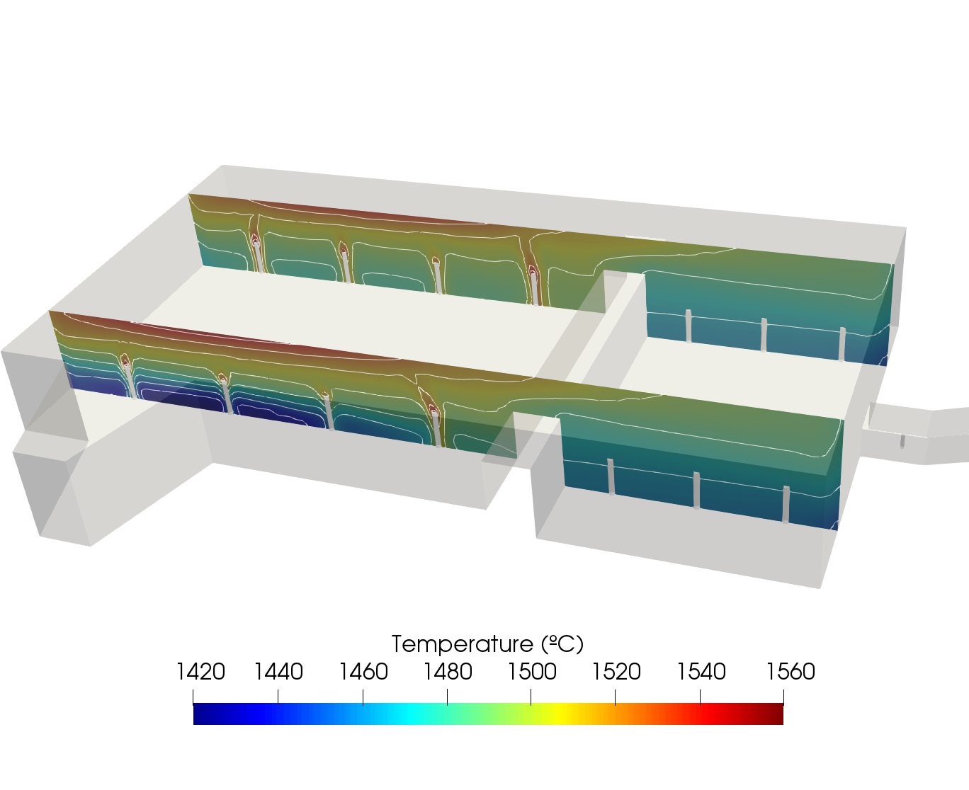
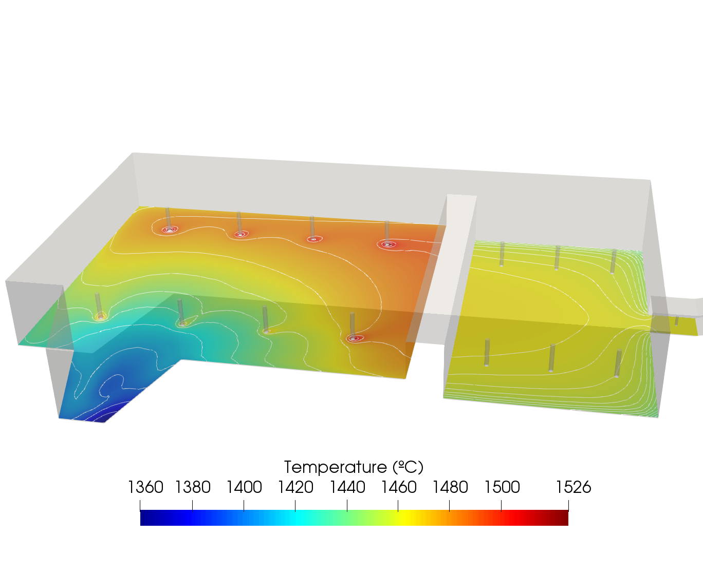
Figure 4: Slides for temperature for the stationary solution.

We further show in Figure 5 the values the Joule heat source generated by the boosters, and defined as $\sigma(\theta)|\phi|^{2}$. We can observe how the heat source is located basically near the booster that are switched on, as expected.

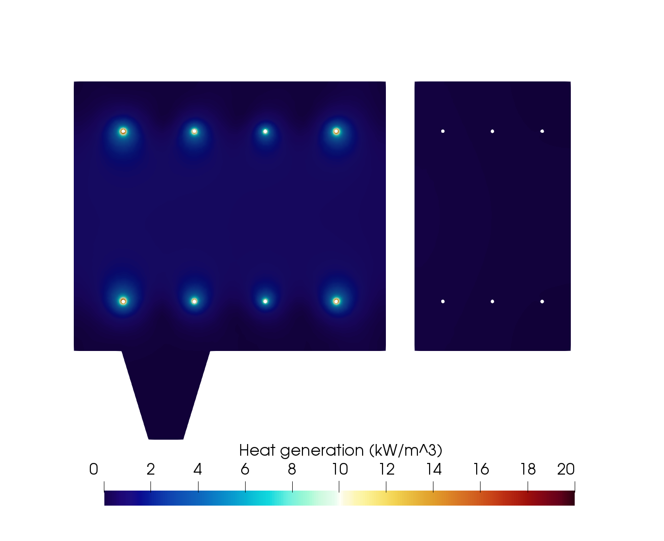
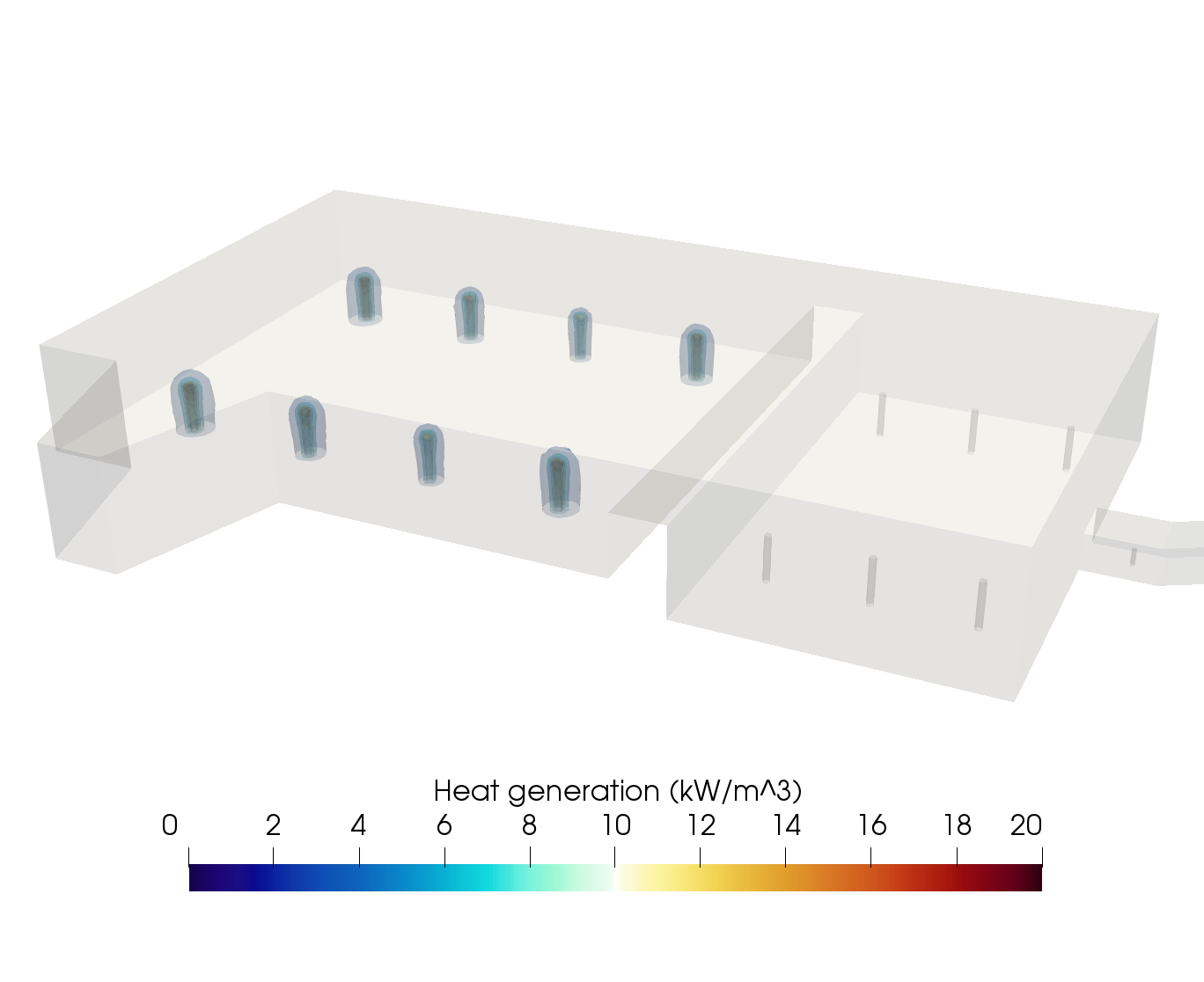
Figure 5: Joule heat source for the stationary solution.

For the velocity, we show some streamlines in Figure 6 (left). As expected, we observe how the vertical velocity increases near the boosters due to the buoyancy forces. This increase of the vertical velocity is higher near the boosters that are further from the inlet. This might be explained by observing that the Joule effect heat source is higher due to the fact the temperature is higher in that zone. We also can observe a recirculation near the wall inside the bulk, that certifies the behavior expected.

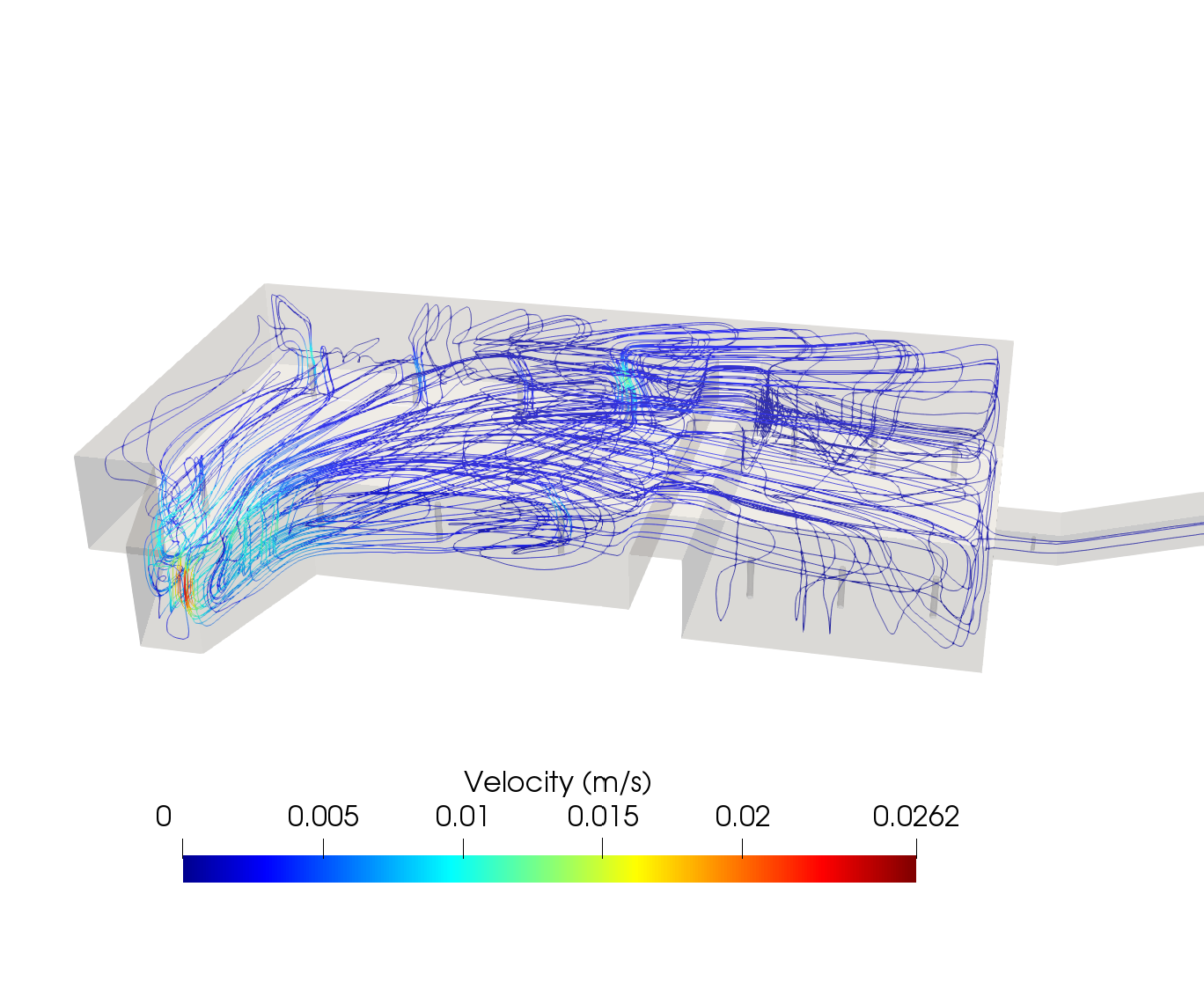
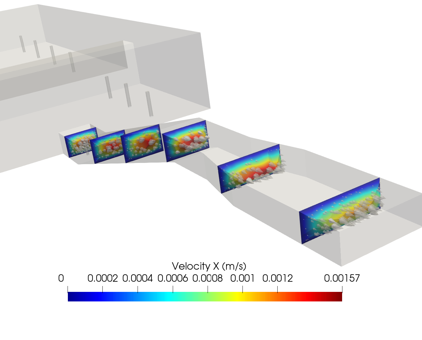
Figure 6: Velocity streamlines (left) and velocity at the throat (right), for the stationary solution.

We want also to highlight the velocity profiles in the throat. In Figure 6 (right) we show some velocity profiles in the throat, where we observe almost a parabolic profile, as expected.

4.2 Numerical results for the air bubbles postprocessing

We next present the numerical results of the postprocessing introduced in section 2.5 to obtain the motion of air bubbles. In the present work, we consider bubbles having different size, released in the first part of the basin, where the granular prime materials are introduced in the furnace.

Figure 7 depicts pathlines of the air bubbles flow fields obtained considering different diameters. From left to right, top to bottom we show the streamlines corresponding with diameters of 1 mm, 0.75 mm, 0.5 mm and 0.25 mm, respectively. All the gas spheres are released at a height of 0.1 m with respect to the furnace base. As it can be observed, practically all bubbles of 1 mm radius escape the top of the fluid. When the diameter become smaller, more proportion of bubbles remain in the furnace. We can observe how, when the diameter is 0.25 mm, due to their smaller rising speed some air spheres go through the throat, remaining in the fluid at the outlet. The simulations and the post processing computation of air bubbles velocity field suggests that the configuration studied would benefit from longer glass latency time, which would allow for smaller air bubbles to abandon the molten material, and eventually improve the final product quality. Since operating conditions of the furnace can be changed in order to increase the glass latency time, this motivates us in introducing parameters affecting operating conditions, and seek computational reduction as discussed in the next section.

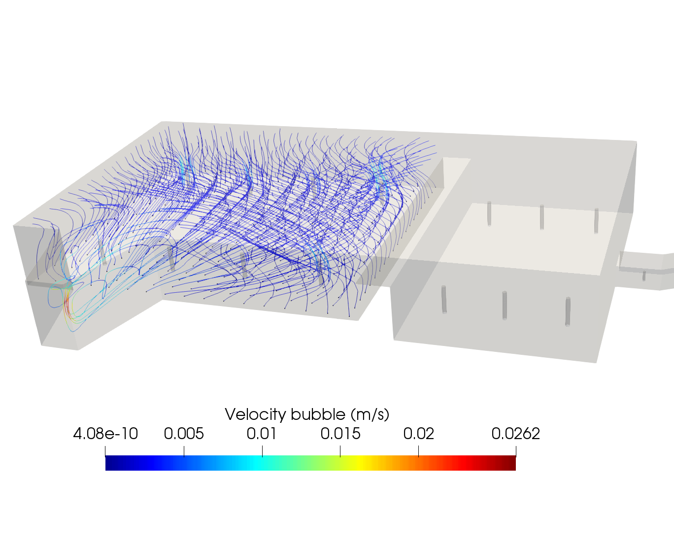
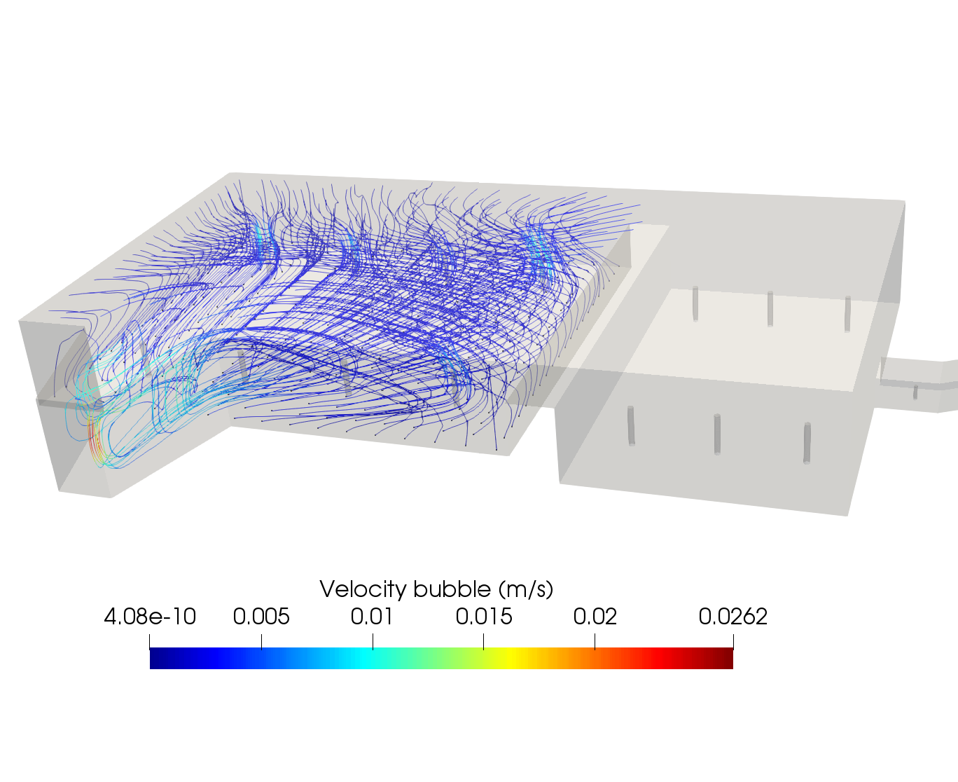
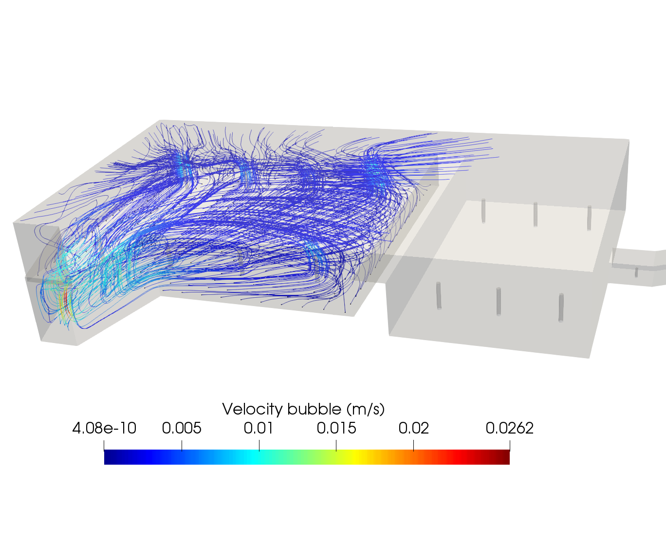
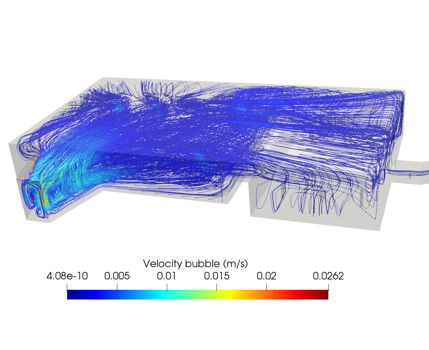
Figure 7: Bubbles streamlines for diameters of 1 mm (top-left), 0.75 mm (top-right), 0.5 mm (bottom-left) and 0.25 mm (bottom-right), for the stationary solution.

5 POD-NN reduced order model

In this section we present a non-intrusive POD for a parametrized PDE, based on a Neural Network. In particular, we consider as parameters the total amount of energy released on the furnace. As explained in previous sections, the energy of the system is introduced in two ways: the heat source relative to the methane combustion, and the heat produced by the booster due to the Joule effect.

Thus, we consider that the total heat flux of combustion, $q_{top}$, on equation (4) ranges on the interval $[240000,300000]kW/(m^{2}s)$, while the voltage, on equation (5), of each of the four pairs of boosters ranges on the interval $[100,160]V$. With this configuration, we are assuming that our parametrized PDE depend on five parameters, which vary in the parameter space $\mathcal{D}=[240000,300000]\times[100,160]^{4}$.

Considering a classical Galerkin POD [14, 21] of problem (8) is hard due to the fact that non-linearities that would force us to employ, for example, a (Discrete) Empirical Interpolation Method (see e.g. [4, 7]), in order to forego employing a Galerkin method and, instead, approximate the different non-linear terms. In order to avoid this, we consider a Neural Network in order to approximate the coefficients of the POD by regression.

First of all, we recall the construction of the POD modes. Let us consider $\mathcal{D}_{train}=\{\boldsymbol{\mu}^{1},\dots,\boldsymbol{\mu}^{P}\}\subset\mathcal{D}$ a set of $P$ parameter values, and the corresponding set of snapshots for each field obtained by collecting the state state solutions corresponding to each parameter value. For simplicity of the notation, in the following we consider only the velocity field and its associated snapshot matrix $S_{\textbf{u}}=\{\textbf{u}(\boldsymbol{\mu}^{1}),\dots,\textbf{u}(\boldsymbol{\mu}^{P})\}$, but in the numerical results we will display ROM results for all solutions fields by proceeding analogously with was is discussed below for the velocity field.

We construct the correlation matrix for each field, given by

$$\mathbf{C}_{ij}=\dfrac{1}{P}(\textbf{u}(\boldsymbol{\mu}^{i}),\textbf{u}(\boldsymbol{\mu}^{j}))_{V},\quad 1\leq i,j\leq P,$$

with $(\cdot,\cdot)_{V}$ a scalar product on $V$. For the definition of the POD modes, we solve the following eigenvalue problem associated to the correlation matrix:

$$\left\{\begin{array}[]{l}\text{Find }(\lambda_{n},\textbf{v}_{n})\in\mathbb{R}\times\mathbb{R}^{P}\text{ such that }\\ \mathbf{C}\textbf{v}_{n}=\lambda_{n}\textbf{v}_{n},\quad 1\leq n\leq P.\end{array}\right.$$ (9)

Solving this problem, we obtain $P$ eigenvalues sorted in descending order, $\lambda_{1}\geq\dots\geq\lambda_{P}$. With the $N$ largest eigenvalues, we define the POD modes as

$$\Psi^{\textbf{u}}_{n}=\displaystyle\sum_{k=1}^{P}(\textbf{v}_{n})_{k}\textbf{u}(\boldsymbol{\mu}^{k}),\quad 1\leq n\leq N,$$ (10)

where we are denoting by $(\textbf{v}_{n})_{k}$ the $k$-th coefficient of the eigenvector $\textbf{v}_{n}\in\mathbb{R}^{P}$. Analogously, we can define the POD modes for pressure ($\Psi_{n}^{p}$), temperature ($\Psi_{n}^{\theta}$), and electric potential ($\Psi^{\phi}_{n}$).

We define the Reduced Order spaces, for velocity, pressure, temperature and electric potential as following

$$\begin{array}[]{ll}V_{N}=\mbox{span}\{\Psi_{n}^{\textbf{u}},\quad 1\leq n\leq N\},&M_{N}=\mbox{span}\{\Psi_{n}^{p},\quad 1\leq n\leq N\},\\ \Theta_{N}=\mbox{span}\{\Psi_{n}^{\theta},\quad 1\leq n\leq N\},&\Phi_{N}=\mbox{span}\{\Psi_{n}^{\phi},\quad 1\leq n\leq N\}.\end{array}$$ (11)

We consider a feed-forward Neural Network in order to build a regression model able to compute efficiently the value of the POD coefficients that better approximate the solution of problem (8). Some previous works on POD-NN can be found in [8, 13, 18]. In that sense, we consider for each parameter value $\boldsymbol{\mu}\in\mathcal{D}$, that the solutions of the NN-POD problem are given by

$$\begin{array}[]{cc}\textbf{u}_{NN}(\boldsymbol{\mu})=\displaystyle\sum_{k=1}^{N}\alpha^{\textbf{u}}_{k}(\boldsymbol{\mu})\Psi_{k}^{\textbf{u}},&p_{NN}(\boldsymbol{\mu})=\displaystyle\sum_{k=1}^{N}\alpha^{p}_{k}(\boldsymbol{\mu})\Psi_{k}^{p},\\ \theta_{NN}(\boldsymbol{\mu})=\displaystyle\sum_{k=1}^{N}\alpha^{\theta}_{k}(\boldsymbol{\mu})\Psi_{k}^{\theta},&\phi_{NN}(\boldsymbol{\mu})=\displaystyle\sum_{k=1}^{N}\alpha^{\phi}_{k}(\boldsymbol{\mu})\Psi_{k}^{\phi},\end{array}$$ (12)

where the coefficients $\alpha^{\textbf{u}}_{k}$, $\alpha^{p}_{k}$, $\alpha^{\theta}_{k}$ and $\alpha^{\phi}_{k}$ are computed as follows (again, for simplicity only for the velocity field). A Neural Network ROM applied to this problem consists on approximate a function $\pi:\mathcal{D}\rightarrow\mathbb{R}^{N}$, that maps each parameter value $\boldsymbol{\mu}\in\mathcal{D}$ to the vector of POD coefficients (for each field):

$$\pi:\boldsymbol{\mu}\in\mathcal{D}\mapsto\boldsymbol{\alpha}^{\textbf{u}}(\boldsymbol{\mu})=(\alpha_{1}^{\textbf{u}}(\boldsymbol{\mu}),\dots,\alpha_{N}^{\textbf{u}}(\boldsymbol{\mu})).$$ (13)

This function $\pi$ is determined through a supervised learning approach, based on a training set given by the pairs $\displaystyle\{(\boldsymbol{\mu}^{k},\pi(\boldsymbol{\mu}^{k}))\}_{k=1}^{P}$. In this work, we have chosen a standard feed-forward Neural Network, which scheme is represented in Figure 8. We consider an input layer of dimension $M$ (the number of parameters considered in our problem), an output of dimension $N$ (the number of POD coefficients to compute), and $L$ inner layers, each compound of $L_{N}$ computing neurons. We set a learning rate $\eta$, the weighted sum as a propagation, the hyperbolic tangent as activation functions, and, in the last layer, the identity as output function. For the learning procedure, we consider a training set of $(2/3)P$ parameter values, and a validation set of $(1/3)P$ parameter values. The network is trained by minimizing a loss function, defined as the mean squared error between the POD-NN and FOM solutions.

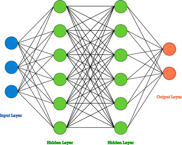
Figure 8: Neural Network with two hidden layers

The reduced order model based on non-intrusive POD-ANN has been implemented in a software tool able to provide real time solution of the fluid dynamic problem for each combination of parameters considered. Figure 9 displays a comparison between the ROM and FOM solutions obtained for a parameter setting corresponding to $283961.719kW/(m^{2}/s)$ of combustion heat flux, and $146.681V$, $116.542V$, $150.134V$, and $106.326V$ for the voltage of each pair of booster, respectively. The plot on the top depicts contours of temperature field predicted with the FOM solver, on three vertical planes within melting the basin. Using an identical layout, the middle plot illustrates the temperature as computed by means of the ROM algorithm. Finally, the bottom plot depicts contours of the relative error between ROM and FOM temperature on the three vertical planes used in the temperature plots. We can observe the similarity of both FOM and ROM solution. Actually, in this case, the maximum of the relative error of both solutions is about $1\%$.

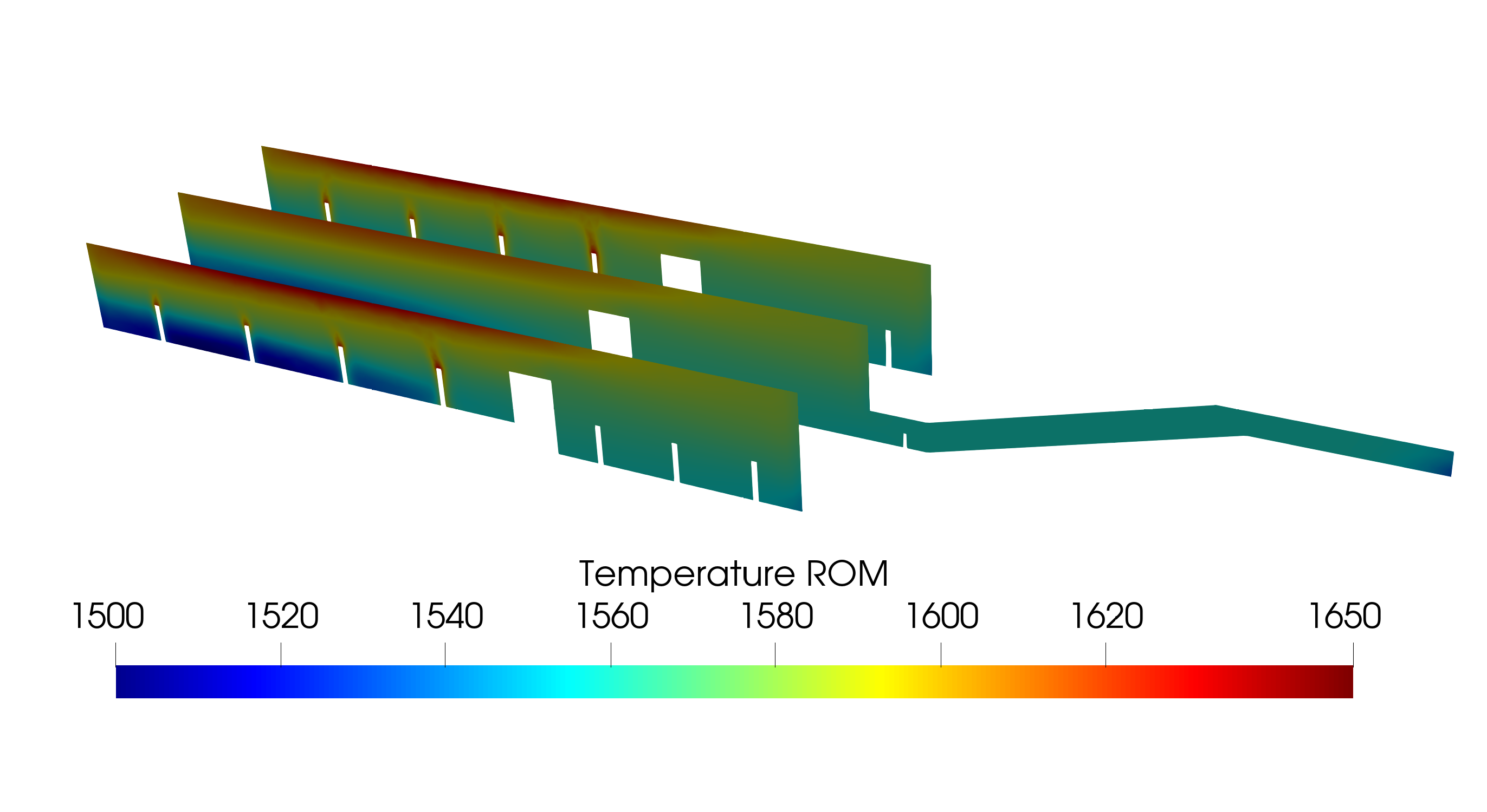
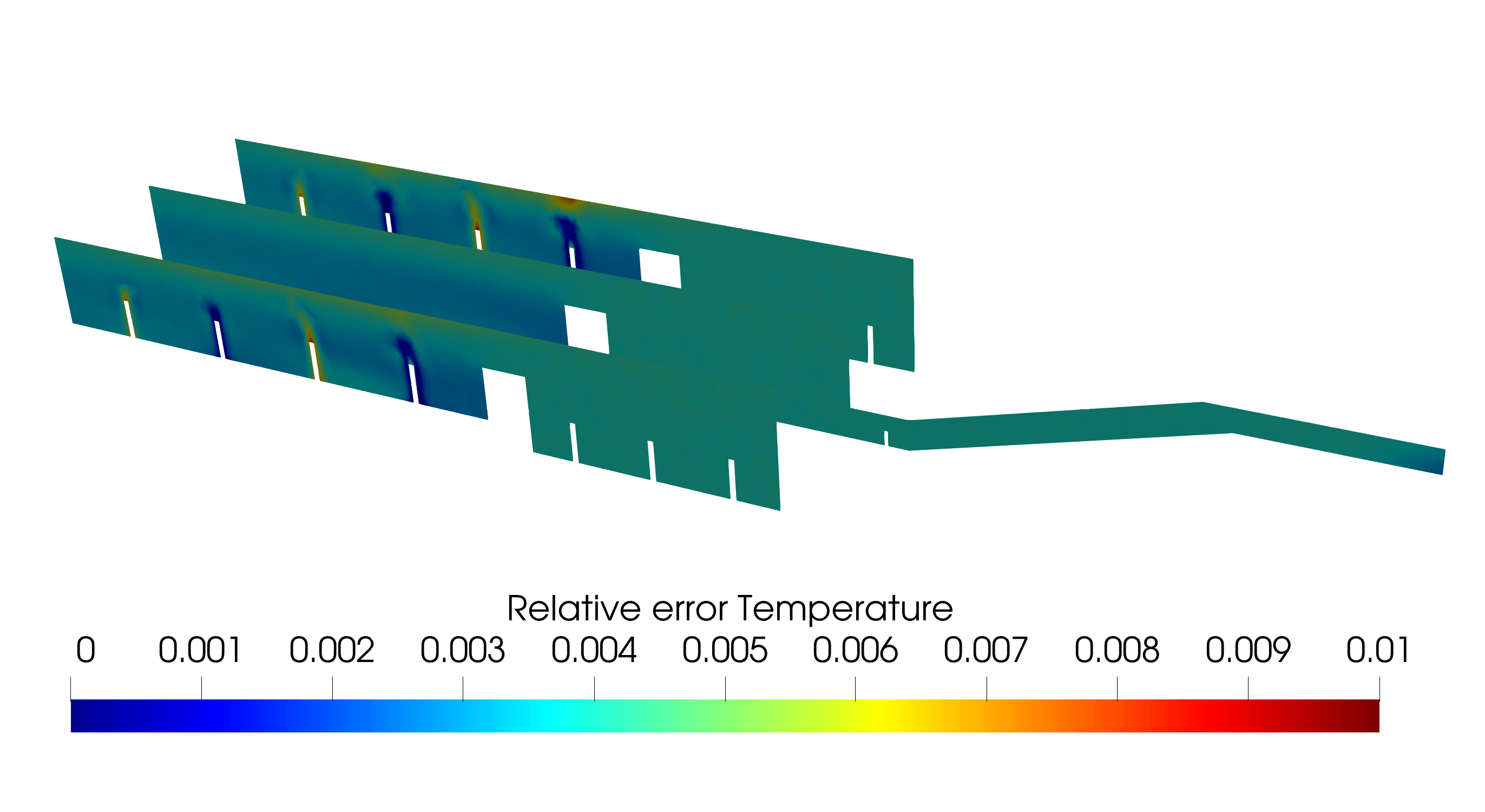
Figure 9: From top to bottom: Temperature of FOM solution, temperature of ROM solution, and the relative error between FOM and ROM of the temperature field. An animation of the solution variations resulting from modification of the value of different process parameters can be viewed at the website https://youtu.be/yRNQaGVmXF4.

We compute the POD-NN relative error, $e_{\textbf{u}},e_{p},e_{\theta},e_{\phi}$, of each field for a given parameter value $\boldsymbol{\mu}\in\mathcal{D}$, given by

$$e_{\textbf{u}}(\boldsymbol{\mu})=\dfrac{\|\textbf{u}_{h}(\boldsymbol{\mu})-\textbf{u}_{NN}(\boldsymbol{\mu})\|}{\|\textbf{u}_{h}(\boldsymbol{\mu})\|},\quad e_{p}(\boldsymbol{\mu})=\dfrac{\|p_{h}(\boldsymbol{\mu})-p_{NN}(\boldsymbol{\mu})\|}{\|p_{h}(\boldsymbol{\mu})\|},$$

$$e_{\theta}(\boldsymbol{\mu})=\dfrac{\|\theta_{h}(\boldsymbol{\mu})-\theta_{NN}(\boldsymbol{\mu})\|}{\|\theta_{h}(\boldsymbol{\mu})\|},\quad e_{\phi}(\boldsymbol{\mu})=\dfrac{\|\phi_{h}(\boldsymbol{\mu})-\phi_{NN}(\boldsymbol{\mu})\|}{\|\phi_{h}(\boldsymbol{\mu})\|}.$$

We consider a set of parameter values, $\mathcal{D}_{train}$, for which we compute the POD-NN relative error. In Figure 10, we show the mean of the POD-NN relative errors for velocity, pressure, temperature and electric potential, depending on the number of POD modes we have considered to construct the reduced spaces. Moreover, in Figure 11, we show the mean of all errors, comparing the order of magnitude of them.

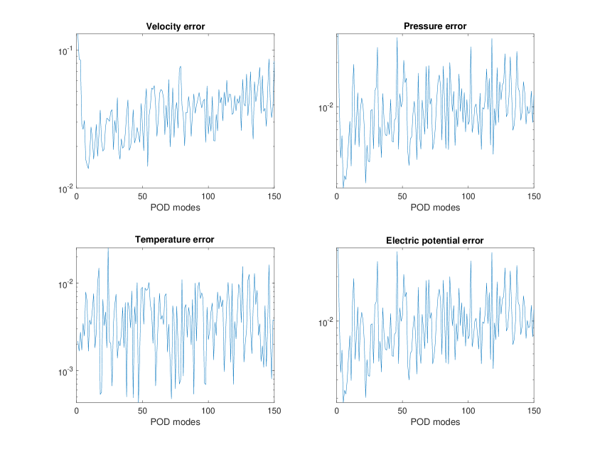
Figure 10: Relative errors for velocity (top left), pressure (top right), temperature (bottom left) and electric potential (bottom right)

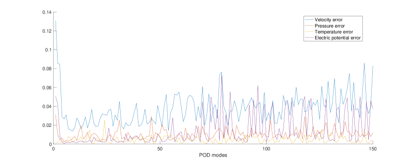
Figure 11: Comparative of relative errors for velocity, pressure, temperature and electric potential.

We can observe that the POD-NN relative error, with respect to the high fidelity solution, ranges between $6\%$ to $1\%$, noticing that the error in temperature is the lowest one. We can observe also a high variability on the mean of the relative error depending on the number of POD modes. That means that we do not need a high number of POD modes in order to have a good approximation, with respect to the high fidelity solution, with the POD-NN approach considered.

6 Conclusions

In this work we have presented the modelling of a 3D flow of a molten glass fluid inside a furnace. We have presented the numerical results of a FEM simulation and compared them with experimental data. We have also modelled the behaviour of air bubbles inside the fluid depending on their size. Moreover, We have performed a POD-NN model with different number of POD modes and we have compared the solution obtained from the non-intrusive POD-NN model with respect to the FE solution. For all the fields, we have obtained an error ranging between $6\%$ and $1\%$, the error in temperature being the lowest one.

References

- [1] A. Abbassi and K. Khoshmanesh, Numerical simulation and experimental analysis of an industrial glass melting furnace, Applied Thermal Engineering, 28 (2008), pp. 450–459.
- [2] D. N. Arnold, F. Brezzi, and M. Fortin, A stable finite element for the Stokes equations, Calcolo, 21 (1984), pp. 337–344.
- [3] F. Ballarin, T. Chacón Rebollo, E. Delgado Ávila, M. Gómez Mármol, and G. Rozza, Certified reduced basis VMS-smagorinsky model for natural convection flow in a cavity with variable height, Computers & Mathematics with Applications, 80 (2020), pp. 973–989.
- [4] M. Barrault, Y. Maday, N. C. Nguyen, and A. T. Patera, An ‘empirical interpolation’ method: application to efficient reduced-basis discretization of partial differential equations, Comptes Rendus Mathematique, 339 (2004), pp. 667–672.
- [5] T. Chacón Rebollo, E. Delgado Ávila, M. Gómez Mármol, F. Ballarin, and G. Rozza, On a certified Smagorinsky reduced basis turbulence model, SIAM Journal on Numerical Analysis, 55 (2017), pp. 3047–3067.
- [6] S.-L. Chang, C. Zhou, and B. Golchert, A numerical investigation of electric heating impacts on solid/liquid glass flow patterns, in 8th AIAA/ASME Joint Thermophysics and Heat Transfer Conference, American Institute of Aeronautics and Astronautics, jun 2002.
- [7] S. Chaturantabut and D. C. Sorensen, Nonlinear model reduction via discrete empirical interpolation, SIAM Journal on Scientific Computing, 32 (2010), pp. 2737–2764.
- [8] W. Chen, Q. Wang, J. S. Hesthaven, and C. Zhang, Physics-informed machine learning for reduced-order modeling of nonlinear problems, Journal of Computational Physics, 446 (2021), p. 110666.
- [9] M. Choudhary, Three-dimensional mathematical model for flow and heat transfer in electric glass furnaces, Heat Transfer Engineering, 6 (1985), pp. 55–65.
- [10] M. K. Choudhary, R. Venuturumilli, and M. R. Hyre, Mathematical modeling of flow and heat transfer phenomena in glass melting, delivery, and forming processes, International Journal of Applied Glass Science, 1 (2010), pp. 188–214.
- [11] R. L. Curran, Mathematical model of an electric glass furnace: Effects of glass color and resistivity, IEEE Transactions on Industry Applications, IA-9 (1973), pp. 348–357.
- [12] C. Giessler and A. Thess, Numerical simulation of electromagnetically controlled thermal convection of glass melt in a crucible, International Journal of Heat and Mass Transfer, 52 (2009), pp. 3373–3389.
- [13] J. Hesthaven and S. Ubbiali, Non-intrusive reduced order modeling of nonlinear problems using neural networks, Journal of Computational Physics, 363 (2018), pp. 55–78.
- [14] K. Kunisch and S. Volkwein, Galerkin proper orthogonal decomposition methods for a general equation in fluid dynamics, SIAM Journal on Numerical Analysis, 40 (2002), pp. 492–515.
- [15] Q. Ma, H. Fang, C. Shang, Z. Liu, and J. Wang, Analysis of melt flows in an electric heating furnace for quartz glass synthesis, in Volume 7: Fluids Engineering, American Society of Mechanical Engineers, nov 2018.
- [16] A. Manzoni, An efficient computational framework for reduced basis approximation and a posteriori error estimation of parametrized Navier-Stokes flows, ESAIM: Mathematical Modelling and Numerical Analysis, 48 (2014), pp. 1199–1226.
- [17] J. Novo and S. Rubino, Error analysis of proper orthogonal decomposition stabilized methods for incompressible flows, SIAM Journal on Numerical Analysis, 59 (2021), pp. 334–369.
- [18] F. Pichi, F. Ballarin, G. Rozza, and J. S. Hesthaven, An artificial neural network approach to bifurcating phenomena in computational fluid dynamics, Computers & Fluids, 254 (2023), p. 105813.
- [19] L. Pilon, G. Zhao, and R. Viskanta, Three-dimensional flow and thermal structures in glass meltingfurnaces. part i. effects of the heat flux distribution, Glass Science and Technology, 75 (2006), pp. 115–124.
- [20] L. Pilon, G. Zhao, and R. Viskanta, Three-dimensional flow and thermal structures in glass meltingfurnaces. part ii. effects of the heat flux distribution, Glass Science and Technology, 75 (2006), pp. 55–68.
- [21] R. Pinnau, Model reduction via proper orthogonal decomposition, in Mathematics in Industry, W. Schilders, H. van der Vorst, and J. Rommes, eds., Springer Berlin Heidelberg, 2008, pp. 95–109.
- [22] A. Quarteroni, Numerical Models for Differential Problems, Springer Milan, 2014.
- [23] A. Quarteroni, A. Manzoni, and F. Negri, Reduced Basis Methods for Partial Differential Equations: An Introduction, Springer, 2015.
- [24] A. Quarteroni, A. Manzoni, and G. Rozza, Certified reduced basis approximation for parametrized partial differential equations and applications, Journal of Mathematics in Industry, 1 (2011).
- [25] J. E. Shelby, Introduction to Glass Science and Technology, Royal Society of Chemistry, 2007.
- [26] R. Viskanta, Review of three-dimensional mathematical modeling of glass melting, Journal of Non-Crystalline Solids, 177 (1994), pp. 347–362.
- [27] W. Xiqi and R. Viskanta, Modeling of heat transfer in the melting of a glass batch, Journal of Non-Crystalline Solids, 80 (1986), pp. 613–622.