Systematic Transmission With Fountain Parity Checks for Erasure Channels With Stop Feedback

Abstract

In this paper, we present new achievability bounds on the maximal achievable rate of variable-length stop-feedback (VLSF) codes operating over a binary erasure channel (BEC) at a fixed message size $M=2^{k}$. We provide new bounds for VLSF codes with zero error, infinite decoding times and with nonzero error, finite decoding times. Both new achievability bounds are proved by constructing a new VLSF code that employs systematic transmission of the first $k$ bits followed by random linear fountain parity bits decoded with a rank decoder. For VLSF codes with infinite decoding times, our new bound outperforms the state-of-the-art result for BEC by Devassy et al. in 2016. We also give a negative answer to the open question Devassy et al. put forward on whether the $23.4\%$ backoff to capacity at $k=3$ is fundamental. For VLSF codes with finite decoding times, numerical evaluations show that the achievable rate for VLSF codes with a moderate number of decoding times closely approaches that for VLSF codes with infinite decoding times.

I Introduction

In a point-to-point communication system with stop feedback, the decoder decides on the fly when to stop transmission and sends a $1$-bit acknowledgement (ACK) or negative acknowledgement (NACK) symbol via the noiseless feedback channel informing the transmitter whether to stop or continue transmission. Meanwhile, the transmitter cannot utilize the stop-feedback symbol to design the next code symbol. Polyanskiy et al. [1] formalized this type of code as the variable-length stop-feedback (VLSF) code. The VLSF code is of practical interest since it includes the hybrid automatic repeat request and incremental redundancy. Polyanskiy et al. showed that even with such a limited use of feedback, the maximal achievable rate of VLSF code is significantly better than that of the fixed-length code in the nonasymptotic regime. Earlier works have also studied various aspects of VLSF codes, including the performance in error-exponent regime [2], performance for random linear codes over the binary erasure channel (BEC) [3], and performance when noisy stop feedback is present [4].

This paper focuses on the BEC with stop feedback and seeks a nonasymptotic achievability bound for the VLSF setup. To the best of our knowledge, Devassy et al. obtained the state-of-the-art achievability [5, Theorem 9] and converse bounds [5, Corollary 6] for VLSF codes operating over a BEC. Note that constructing VLSF codes for the BEC is equivalent to constructing rateless erasure codes. Motivated by this observation, Devassy et al. derived the achievability bound by analyzing a family of random linear fountain codes [6, Chapter 50] of message size $2^{k}$ and by using a rank decoder. The rank decoder keeps track of the rank of the generator matrix associated with unerased received symbols. As soon as the rank equals $k$, the decoder stops transmission by sending an ACK symbol and reproduces the $k$-bit message with zero error using the inverse of the generator matrix. However, their achievability bound implies that the ratio of maximal achievable rate to capacity is only a function of message length $k$ and the ratio attains the maximum of $76.6\%$ at $k=3$. Hence, they posed the question whether the $23.4\%$ backoff percentage to capacity at $k=3$ is fundamental.

Unlike Devassy et al.’s approach, we adopt a new coding scheme called systematic transmission followed by random linear fountain coding (ST-RLFC). Namely, the transmitter simply transmits the first $k$ message bits in the first $k$ time instants. After that, the transmitter employs a random linear fountain code to generate parity bits. Specifically, starting the $(k+1)$th time instant, both the encoder and decoder select the same nonzero base vector in $\{0,1\}^{k}$ according to the common randomness. The encoder produces the code symbol by linearly combining the message bits using the selected base vector. The decoder is still the same rank decoder.

Our contributions in this paper are as follows.

• By analyzing the ST-RLFC scheme, we present a new achievability bound for VLSF codes of message size $M=2^{k}$ and zero error probability. Our new bound outperforms Devassy et al.’s result [5, Theorem 9]. In addition, the new bound implies that the $23.4\%$ backoff percentage to capacity reported by Devassy et al. is not fundamental. On the contrary, the new bound indicates that the backoff percentage is proportional to the erasure probability at any given message length $k$. If the erasure probability is zero, there is no backoff from capacity.

• The new VLSF achievability bound for zero-error VLSF codes implies a new achievability bound for VLSF codes constrained to have finite decoding times and a nonzero error probability. Numerical computations show that when number of decoding times $m$ is small, a slight increase in $m$ can dramatically improve the achievable rate. However, when $m$ is moderately large (for instance, $m=16$ for erasure probability $0.5$), the achievable rate closely approaches that for $m=\infty$.

The remainder of this paper is organized as follows. Section II introduces the notation and the VLSF code, and presents previously known bounds for VLSF codes operating over a BEC. Section III provides the new VLSF achievability bound and its implications. Section IV includes proofs of the main results. Section V concludes the paper.

II Preliminaries

II-A Notation

Let $\mathbb{N}=\{0,1,\dots\}$, $\mathbb{N}_{+}=\mathbb{N}\setminus\{0\}$, $\mathbb{N}_{\infty}=\mathbb{N}\cup\{\infty\}$ be the set of natural numbers, positive integers, and extended natural numbers, respectively. For $i\in\mathbb{N}$, $[i]\triangleq\{1,2,\dots,i\}$. We use $x_{i}^{j}$ to denote a sequence $(x_{i},x_{i+1},\dots,x_{j})$, $1\leq i\leq j$. We denote by $\bm{e}_{i}\in\mathbb{R}^{k\times 1}$ the $k$-dimensional natural base vector with $1$ at index $i$ and $0$ everywhere else, $1\leq i\leq k$. We denote the distribution of a random variable $X$ by $\mathsf{P}_{X}$.

II-B VLSF Codes

We consider a BEC with input alphabet $\mathcal{X}=\{0,1\}$, output alphabet $\mathcal{Y}=\{0,?,1\}$, and erasure probability $p\in[0,1)$. A VLSF code for BEC with finite decoding times is defined as follows.

Definition 1

An $(l,n_{1}^{m},M,\epsilon)$ VLSF code, where $l>0$, $m\in\mathbb{N}_{\infty}$, $n_{1}^{m}\in\mathbb{N}^{m}$ satisfying $n_{1}<n_{2}<\cdots<n_{m}$, $M\in\mathbb{N}_{+}$, and $\epsilon\in(0,1)$, is defined by:

• A finite alphabet $\mathcal{U}$ and a probability distribution $\mathsf{P}_{U}$ on $\mathcal{U}$ defining the common randomness random variable $U$ that is revealed to both the transmitter and the receiver before the start of the transmission.

• A sequence of encoders $f_{n}:\mathcal{U}\times[M]\to\mathcal{X}$, $n=1,2,\dots,n_{m}$, defining the channel inputs

  $$X_{n}=f_{n}(U,W),$$ (1)

  where $W\in[M]$ is the equiprobable message.

• A non-negative integer-valued random stopping time $\tau\in\{n_{1},n_{2},\dots,n_{m}\}$ of the filtration generated by $\{U,Y^{n_{i}}\}_{i=1}^{m}$ that satisfies the average decoding time constraint

  $$\mathbb{E}[\tau]\leq l.$$ (2)

• $m$ decoding functions $g_{n_{i}}:\mathcal{U}\times\mathcal{Y}^{n_{i}}\to[M]$, providing the best estimate of $W$ at time $n_{i}$, $i\in[m]$. The final decision $\hat{W}$ is computed at time instant $\tau$, i.e., $\hat{W}=g_{\tau}(U,Y^{\tau})$ and must satisfy the average error probability constraint

  $$P_{e}\triangleq\mathbb{P}[\hat{W}\neq W]\leq\epsilon.$$ (3)

Comparing to Polyanskiy et al.’s VLSF code definition [1], the primary distinctions are two-fold. First, the VLSF code is allowed to have finite decoding times rather than infinite decoding times. As a result, the stopping time is constrained within these decoding times. Second, both the expected blocklength and error probability constraints correspond to the given sequence of decoding times rather than $\mathbb{N}$.

In this paper, we focus on upper bounding the average blocklength $\mathbb{E}[\tau]$ of $(l,\mathbb{N},2^{k},0)$ VLSF code with $m=\infty$ and $(l,n_{1}^{m},2^{k},\epsilon)$ VLSF code with $m<\infty$. The rate of an $(l,n_{1}^{m},M,\epsilon)$ VLSF code is defined by

$$R\triangleq\frac{\log M}{\mathbb{E}[\tau]}.$$ (4)

II-C Previous Results for VLSF Codes over BECs

For the BEC, the decoder has the ability to identify the correct message whenever only a single codeword is compatible with the unerased channel outputs up to that point. By exploiting this fact and utilizing the RLFC, Devassy et al. [5] obtained state-of-the-art achievability bound for zero-error VLSF codes with message size $M$ that is a power of $2$.

Theorem 1 (Theorem 9, [5])

For each integer $k\geq 1$, there exists an $(l,\mathbb{N},2^{k},0)$ VLSF code for a BEC$(p)$ with

$$l\leq\frac{1}{C}\left(k+\sum_{i=1}^{k-1}\frac{2^{i}-1}{2^{k}-2^{i}}\right),$$ (5)

Note that the second term in parentheses of (5) is bounded by the Erdös-Borwein constant $c=1.60669515...$ (OEIS: A065442),

$$\sum_{i=1}^{k-1}\frac{2^{i}-1}{2^{k}-2^{i}}\leq\sum_{j=1}^{k-1}\frac{1}{2^{j}-1}\leq\sum_{j=1}^{\infty}\frac{1}{2^{j}-1}=c.$$ (6)

In [3, Theorem 2], Heidarzadeh et al. showed that by constructing random linear codes for which column vectors of the parity check matrix for erased symbols are linearly independent, the average blocklength of the corresponding $(l,\mathbb{N},2^{k},0)$ VLSF code is given by $\frac{k+c}{C}$. This indicates that Heidarzadeh’s random linear coding scheme performs as good as Devassy’s RLFC scheme for sufficiently large message length $k$.

The state-of-the-art converse bound for $(l,\mathbb{N},2^{k},0)$ VLSF codes over a BEC is also obtained by Devassy et al. using the method of binary sequential hypothesis testing.

Theorem 2 (Corollary 6, [5])

The minimum average blocklength $l_{f}^{*}(M,0)$ of an $(l,\mathbb{N},M,0)$ VLSF code over a BEC$(p)$ is given by

$$l^{*}_{f}(M,0)=\frac{\lfloor\log_{2}M\rfloor+2\left(1-2^{\lfloor\log_{2}M\rfloor-\log_{2}M}\right)}{C}.$$ (7)

Note that when $M$ is a power of $2$, Theorem 2 implies that the converse bound on maximal achievable rate is simply the capacity of the BEC.

III Achievable Rates of VLSF codes over BECs

In this section, we present a new coding scheme for a BEC called the ST-RLFC, a new achievability bound for zero-error VLSF codes of infinite decoding times, and the comparison with Devassy et al.’s result. Finally, we present a new achievability bound for VLSF code with finite decoding times and a comparison of achievability bounds for various numbers of decoding times.

III-A ST-RLFC Scheme

Consider transmitting a $k$-bit message

$$\bm{b}=(b_{1},b_{2},\dots,b_{k})\in\{0,1\}^{k}.$$ (8)

Let us define the set of nonzero base vectors in $\{0,1\}^{k}$ by

$$\mathcal{G}_{k}\triangleq\{\bm{v}\in\{0,1\}^{k}:\bm{v}\neq\bm{0}\}.$$ (9)

Using ST-RLFC scheme, the channel input at time instant $n\in\mathbb{N}_{+}$ for message $\bm{b}$ is given by

$$X_{n}=\begin{cases}b_{n},&\text{if }1\leq n\leq k\\ \bigoplus_{i=1}^{k}g_{n,i}b_{i}&\text{if }n>k,\end{cases}$$ (10)

where $\oplus$ denotes bit-wise exclusive-or (XOR) operator, and $\bm{g}_{n}=(g_{n,1},g_{n,2},\dots,g_{n,k})^{\top}\in\mathcal{G}_{k}$ is generated at time instant $n$ according to a uniformly distributed random variable $\tilde{U}\in\mathcal{G}_{k}$. Note that the encoder and decoder share the same common random variable $\tilde{U}$ at time instant $n>k$ so that the decoder can produce the same $\bm{g}_{n}$ at time $n$. For $1\leq n\leq k$, both the encoder and decoder simply use the natural base vector $\bm{e}_{n}\in\mathbb{R}^{k\times 1}$. For all $\bm{b}\in\{0,1\}^{k}$, the procedure (10) specifies the common codebook before the start of transmission, i.e., the common randomness random variable $U$ in Definition 1.

Let $Y_{n}$ be the received symbol after transmitting $X_{n}$ over a BEC$(p)$, $p\in[0,1)$. We consider the rank decoder [5] that keeps track of the rank of generator matrix $G$ associated with received symbols $Y^{n}=(Y_{1},Y_{2},\dots,Y_{n})$. Let $G(n)$ denote the $n$th column of $G$. If $Y_{n}=?$, $G(n)=\bm{0}$; otherwise, $G(n)=\bm{g}_{n}$. Define the stopping time

$$\tau\triangleq\inf\{n\in\mathbb{N}:\text{$G(1:n)$ has rank $k$}\},$$ (11)

where $G(i:j)$ denotes the matrix formed by column vectors from time instants $i$ to $j$, $1\leq i\leq j$. Thus, the rank decoder stops transmission at time instant $\tau$ and reproduces the $k$-bit message $\bm{b}$ using $Y^{\tau}$ and the inverse of $G(1:\tau)$ (namely, by solving $k$ message bits from $k$ linearly independent equations). Clearly, the error probability associated with the ST-RLFC scheme is zero.

III-B Achievability of Zero-Error VLSF Codes

The ST-RLFC scheme implies the following achievability bound for $(l,\mathbb{N},2^{k},0)$ VLSF codes operating over a BEC.

Theorem 3

For a given integer $k\geq 1$, there exists an $(l,\mathbb{N},2^{k},0)$ VLSF code for BEC$(p)$, $p\in[0,1)$, with

$$l\leq k+\frac{1}{C}\sum_{i=0}^{k-1}\frac{2^{k}-1}{2^{k}-2^{i}}F(i;k,1-p).$$ (12)

where $C=1-p$ and

$$F(i;k,1-p)\triangleq\sum_{j=0}^{i}\binom{k}{j}(1-p)^{j}p^{k-j}$$ (13)

denotes the CDF evaluated at $i$, $0\leq i\leq k$, of a binomial distribution with $k$ trials and success probability $1-p$.

Proof:

See Section IV-A. ∎

For non-vanishing error probability $\epsilon>0$, using Polyanskiy’s early termination scheme in [1, Section III-D] by stopping the zero-error VLSF code at $\tau=0$ with probability $\epsilon$, the corresponding achievability bound can be readily obtained by multiplying the right-hand side (RHS) of (12) by a factor $(1-\epsilon)$.

We remark that the new achievability bound (12) is tighter than Devassy’s bound (5) and two bounds are equal if $p=1$ or $k=1$. This is stated in the following corollary.

Corollary 1

For a given $k\in\mathbb{N}_{+}$ and BEC$(p)$, $p\in[0,1]$, it holds that

$$kC+\sum_{i=0}^{k-1}\frac{2^{k}-1}{2^{k}-2^{i}}F(i;k,1-p)\leq k+\sum_{i=1}^{k-1}\frac{2^{i}-1}{2^{k}-2^{i}},$$ (14)

where $C=1-p$ and $F(i;k,1-p)$ is given by (13). Equality holds if $p=1$ or $k=1$.

Proof:

Fix $k\in\mathbb{N}_{+}$ and $p\in[0,1]$. First, note that

$$k+\sum_{i=1}^{k-1}\frac{2^{i}-1}{2^{k}-2^{i}}=\sum_{i=0}^{k-1}\frac{2^{k}-1}{2^{k}-2^{i}}.$$ (15)

Hence,

$$\sum_{i=0}^{k-1}\frac{2^{k}-1}{2^{k}-2^{i}}-\sum_{i=0}^{k-1}\frac{2^{k}-1}{2^{k}-2^{i}}F(i;k,1-p)-k(1-p)$$

$$=\sum_{i=0}^{k-1}\frac{2^{k}-1}{2^{k}-2^{i}}F^{c}(i;k,1-p)-k(1-p)$$ (16)

$$\geq\sum_{i=0}^{k-1}F^{c}(i;k,1-p)-k(1-p)$$ (17)

$$=0,$$

where in (17), $F^{c}(\cdot)\triangleq 1-F(\cdot)$ denotes the tail probability, and the sum of tail probability equals the expectation $k(1-p)$. Note that (16) equals $0$ if $p=1$ or $k=1$. This completes the proof of Corollary 1. ∎

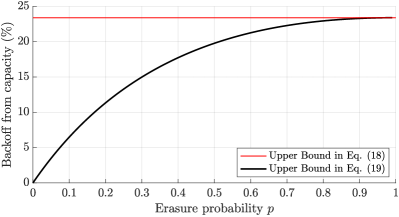
Figure 1: Percentage of backoff from the capacity of BEC for $k=3$. The red curve corresponds to a backoff percentage $23.4\%$.

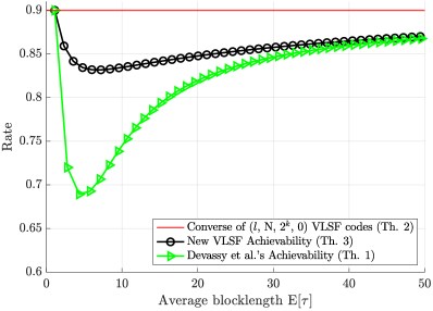
Figure 2: Rate vs. average blocklength $\mathbb{E}[\tau]$ for $(l,\mathbb{N},2^{k},0)$ VLSF codes operated over the BEC$(0.1)$. The markers correspond to integer message lengths.

For BEC$(0)$ and $k\geq 2$, our new bound (12) reduces to $k$, whereas Devassy et al’s bound (5) is strictly larger than $k$ and approaches $k+c$ for sufficiently large $k$, where $c$ denotes the Erdös-Borwein constant. Moreover, (5) also implies an upper bound independent of $p$ on the backoff percentage to capacity,

$$1-\frac{R}{C}\leq 1-\frac{k}{k+\sum_{i=1}^{k-1}\frac{2^{i}-1}{2^{k}-2^{i}}}.$$ (18)

Devassy et al. [5] reported that this upper bound attains its maximum $23.4\%$ at $k=3$ and that the maximum is independent of erasure probability, thus raising the question whether this backoff percentage is fundamental. In contrast, our result in (12) implies a refined upper bound on backoff percentage that is dependent on $p$,

$$1-\frac{R}{C} \leq 1-\frac{k}{\sum_{i=0}^{k-1}\frac{2^{k}-1}{2^{k}-2^{i}}F(i;k,1-p)+k(1-p)}.$$ (19)

Fig. 1 shows the comparison of these two upper bounds at $k=3$. We see that for $k=3$, the upper bound in (19) is a strictly increasing function of $p$. As $p\to 0$, this upper bound converges to $0$, which closes the backoff from capacity at $k=3$. As $p\to 1$, the upper bound in (19) converges to the backoff percentage in (18), as shown in Corollary 1.

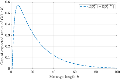
Figure 3: $\mathbb{E}[S^{\text{ST}}_{k}]-\mathbb{E}[S^{\text{RLFC}}_{k}]$ vs. $k$ for BEC$(0.1)$, where $k$ ranges from $1$ to $100$.

Fig. 2 shows the comparison between the new achievability bound (Theorem 3) and Devassy et al.’s bounds (Theorems 1 and 2) for BEC$(0.1)$. As can be seen, for a small message length, the new achievability bound is closer to capacity than Devassy et al.’s bound. This is because when $k$ is small, systematic transmission of the uncoded message symbol is more likely to increase rank than transmitting a fountain code symbol. However, as $k$ gets larger, the advantage of systematic transmission over RLFC gradually diminishes. To see this more clearly, let random variables $S^{\text{ST}}_{k}$ and $S^{\text{RLFC}}_{k}$ denote the rank of generator matrix $G(1:k)$ for ST and RLFC, respectively. We use $\mathbb{E}[S^{\text{ST}}_{k}]-\mathbb{E}[S^{\text{RLFC}}_{k}]$ as the metric to measure the difference of rank increase rate over time range $1$ to $k$. Note that $\mathbb{E}[S^{\text{ST}}_{k}]=k(1-p)$ since the rank distribution at time instant $k$ is binomial. $\mathbb{E}[S^{\text{RLFC}}_{k}]$ can be numerically computed using the one-step transfer matrix $P$ in (32) and initial distribution $[1,\bm{0}^{\top}]\in\mathbb{R}^{1\times(k+1)}$. Fig. 3 shows $\mathbb{E}[S^{\text{ST}}_{k}]-\mathbb{E}[S^{\text{RLFC}}_{k}]$ as a function of message length $k$ for BEC$(0.1)$. We see that this gap constantly remains nonnegative, implying that the rank increase rate for ST is always faster than that for RLFC. For sufficiently large $k$, this gap becomes small, indicating the diminishing advantage of ST over RLFC.

III-C Achievability of VLSF Codes with Finite Decoding Times

The ST-RLFC scheme also facilitates an $(l,n_{1}^{m},2^{k},\epsilon)$ VLSF code for a BEC. This code is constructed by using the same ST-RLFC scheme in (10) but a rank decoder that only considers a finite set of decoding times. Specifically, fix $n_{1}^{m}\in\mathbb{N}_{+}$ satisfying $n_{1}<n_{2}<\cdots<n_{m}$. For a given $k\in\mathbb{N}_{+}$ and $\epsilon\in(0,1)$, the rank decoder still shares the same common randomness with the encoder in selecting the base vector $\bm{g}_{n}$, except that it now adopts the following stopping time:

$$\tau^{*}\triangleq\inf\{n\in\{n_{i}\}_{i=1}^{m}:G(1:n)\text{ has rank $k$ or $n=n_{m}$}\}.$$ (20)

If $\tau\leq n_{m}$ and $G(1:\tau)$ is full rank, the rank decoder reproduces the transmitted message using $Y^{\tau}$ and the inverse of $G(1:\tau)$. If $\tau=n_{m}$ and $G(1:n_{m})$ is rank deficient, then the rank decoder outputs an arbitrary message.

The ST-RLFC scheme and the modified rank decoder imply the following achievability bound for an $(l,n_{1}^{m},2^{k},\epsilon)$ VLSF code.

Theorem 4

Fix $n_{1}^{m}\in\mathbb{N}_{+}^{m}$ satisfying $n_{1}<n_{2}<\cdots<n_{m}$. For any positive integer $k\in\mathbb{N}_{+}$ and $\epsilon\in(0,1)$, there exists an $(l,n_{1}^{m},2^{k},\epsilon)$ VLSF code for the BEC$(p)$ with

$$l \leq n_{m}-\sum_{i=1}^{m-1}(n_{i+1}-n_{i})\mathbb{P}[S_{n_{i}}=k],$$ (21)

$$\epsilon \leq 1-\mathbb{P}[S_{n_{m}}=k],$$ (22)

where the random variable $S_{n}$ denote the rank of the generator matrix $G(1:n)$ observed by the rank decoder. Specifically, $\mathbb{P}[S_{n}=k]$ is given by

$$\mathbb{P}[S_{n}=k]=\begin{cases}0,&\text{if }n<k\\ 1-\bm{\alpha}^{\top}T^{n-k}\bm{1},&\text{if }n\geq k,\end{cases}$$ (23)

where $\bm{\alpha}=[\alpha_{1},\alpha_{2},\dots,\alpha_{k}]^{\top}\in\mathbb{R}^{k\times 1}$ with $\alpha_{i}=F(i;k,1-p)$, $0\leq i\leq k-1$, and $F(i;k,1-p)$ is given by (13), $T\in\mathbb{R}^{k\times k}$ with entries given by

$$T_{i,i} =p+\frac{(1-p)(2^{i-1}-1)}{2^{k}-1},$$ (24)

$$T_{i,i+1} =\frac{(1-p)(2^{k}-2^{i-1})}{2^{k}-1},$$ (25)

$$T_{i,j} =0,\text{ for }j\neq i\text{ and }j\neq i+1.$$ (26)

Proof:

See Section IV-B. ∎

Theorem 4 facilitates an integer program that can be used to compute the achievability bound on rate for all zero-error VLSF codes of message size $M=2^{k}$ and $m$ decoding times. Define

$$N(n_{1}^{m}) \triangleq n_{m}-\sum_{i=1}^{m-1}(n_{i+1}-n_{i})\mathbb{P}[S_{n_{i}}=k].$$ (27)

For a given number of decoding times $m\in\mathbb{N}_{+}$, message length $k\in\mathbb{N}_{+}$, and a target error probability $\delta\in(0,1)$,

$$\begin{split}\min_{n_{1}^{m}}&\quad N(n_{1}^{m})\\ \operatorname{s.t.}&\quad 1-\mathbb{P}[S_{n_{m}}=k]\leq\delta\end{split}$$ (28)

Assume $N(a_{1}^{m})$ is the minimum value after solving (28), where $a_{1}^{m}$ is the minimizer. Then the achievability bound on rate for a VLSF code of message size $2^{k}$, target error probability $\delta$, and $m$ decoding times is given by $\frac{k}{N(a_{1}^{m})}$. For reasonably small values of $m$, one can use brute-force method to obtain $a_{1}^{m}$ and $N(a_{1}^{m})$.

For BEC$(0.5)$, Fig. 4 shows achievability bounds for $(l,n_{1}^{m},2^{k},\delta)$ VLSF codes, where $m\in\{1,2,4,8,16\}$ and target error probability $\delta=10^{-3}$. The adjusted achievability bound boosted by $\frac{1}{1-\delta}$ for $m=\infty$ using Theorem 3 and Polyanskiy’s early termination scheme is also shown. We see that when $m$ is small, increasing $m$ can dramatically improve the achievable rate. However, when $m=16$, the achievable rate closely approaches that for $m=\infty$. We remark that similar effect on achievable rate by the varying number of decoding times has also been observed in several previous works, e.g., [3, 7, 8].

IV Proofs

In this section, we prove our main results.

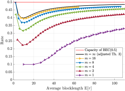
Figure 4: Rate vs. average blocklength $\mathbb{E}[\tau]$ for $(l,n_{1}^{m},2^{k},\delta)$ VLSF codes operated over the BEC$(0.5)$, where $\delta=10^{-3}$. The marker corresponds to integer message length $k$. In this figure, $k\geq 1$ for $m=1,2,4,8$ and $k\geq 2$ for $m=16$. Legend “adjusted Th. 3” means that the upper bound on $l$ is the RHS of (12) multiplied by $(1-\delta)$.

IV-A Proof of Theorem 3

Let random variable $S_{n}$ denote the rank of generator matrix $G(1:n)$. According to the ST-RLFC scheme, the probability mass function (PMF) of $S_{k}$ at time $k$ is given by

$$\mathbb{P}[S_{k}=r]=\binom{k}{r}(1-p)^{r}p^{k-r},\quad 0\leq r\leq k.$$ (29)

For $n\geq k$, due to the BEC$(p)$ and our RLFC scheme, $S_{n+1}=S_{n}=r$ occurs if $Y_{n+1}=?$ or if $Y_{n+1}\neq?$ and $\bm{g}_{n+1}$ is a linear combination of previous $r$ independent base vectors. Otherwise, $S_{n+1}=r+1$. Hence, the behavior of $S_{n}$, $n\geq k$, is characterized by the following discrete-time homogeneous Markov chain with $k+1$ states.

$$\mathbb{P}[S_{n+1}=r|S_{n}=r]=p+\frac{(1-p)(2^{r}-1)}{2^{k}-1},$$ (30)

$$\mathbb{P}[S_{n+1}=r+1|S_{n}=r]=\frac{(1-p)(2^{k}-2^{r})}{2^{k}-1},$$ (31)

where $0\leq r\leq k-1$, and $\mathbb{P}[S_{n+1}=k|S_{n}=k]=1$. Note that this Markov chain has a single absorbing state $S_{n}=k$. The time to absorption for this Markov chain follows a discrete phase-type distribution [9, Chapter 2]. More specifically, the one-step transfer matrix $P\in\mathbb{R}^{(k+1)\times(k+1)}$ of this Markov chain can be written as

$$P=\begin{bmatrix}T&\bm{t}\\ \bm{0}^{\top}&1\end{bmatrix},$$ (32)

where the entries of $T\in\mathbb{R}^{k\times k}$ are given by

$$T_{i,i} =p+\frac{(1-p)(2^{i-1}-1)}{2^{k}-1},$$ (33)

$$T_{i,i+1} =\frac{(1-p)(2^{k}-2^{i-1})}{2^{k}-1},$$ (34)

and $T_{i,j}=0$ for any other pair $(i,j)$, $1\leq i,j\leq k$. Since $P$ is a stochastic matrix, it follows that

$$\bm{t}=(I-T)\bm{1}.$$ (35)

The initial probability distribution is given by $[\bm{\alpha}^{\top},\alpha_{k}]$, where

$$\bm{\alpha}^{\top}\triangleq\begin{bmatrix}\mathbb{P}[S_{k}=0]&\mathbb{P}[S_{k}=1]&\cdots&\mathbb{P}[S_{k}=k-1]\end{bmatrix},$$ (36)

with $\mathbb{P}[S_{k}=r]$ given by (29), and $\alpha_{k}=1-\bm{\alpha}^{\top}\bm{1}$. Let random variable $X\in\mathbb{N}$ denote the time to absorbing state $k$ with initial distribution $[\bm{\alpha}^{\top},\alpha_{k}]$. Hence, it follows that $X$ has PMF

$$\mathbb{P}[X=n]=\bm{\alpha}^{\top}T^{n-1}\bm{t},\quad n\in\mathbb{N}_{+},$$ (37)

and $\mathbb{P}[X=0]=\alpha_{k}$. Define the generating function of $X$ by

$$H_{X}(z) \triangleq\mathbb{E}[z^{X}]=\sum_{n=0}^{\infty}z^{n}\mathbb{P}[X=n]$$

$$=\alpha_{k}+\sum_{n=1}^{\infty}z^{n}\bm{\alpha}^{\top}T^{n-1}\bm{t}$$

$$=\alpha_{k}+z\bm{\alpha}^{\top}\left(\sum_{n=0}^{\infty}(zT)^{n}\right)\bm{t}$$ (38)

$$=\alpha_{k}+z\bm{\alpha}^{\top}(I-zT)^{-1}(I-T)\bm{1},$$ (39)

where in (38), we have used $\sum_{n=0}^{\infty}A^{n}=(I-A)^{-1}$ whenever $|\lambda_{i}|<1$ for all $i\in[k]$, where $\{\lambda_{i}\}_{i=1}^{k}$ denotes the eigenvalues of a square matrix $A\in\mathbb{R}^{k\times k}$. Hence, the expected time to absorbing state $k$ is given by

$$\mathbb{E}[X] =\frac{\mathop{}\!\mathrm{d}H_{X}(z)}{\mathop{}\!\mathrm{d}z}\Big{|}_{z=1}=\bm{\alpha}^{\top}(I-T)^{-1}\bm{1}.$$ (40)

Therefore, the expected stopping time $\mathbb{E}[\tau]$, with $\tau$ defined in (11), is given by

$$\mathbb{E}[\tau] =k+\mathbb{E}[X]$$

$$=k+\bm{\alpha}^{\top}(I-T)^{-1}\bm{1}$$ (41)

Note that

$$I-T =(1-p)\operatorname{diag}\left(1,\frac{2^{k}-2^{1}}{2^{k}-1},\frac{2^{k}-2^{2}}{2^{k}-1},\cdots,\frac{2^{k}-2^{k-1}}{2^{k}-1}\right)$$

$$\phantom{==}\cdot\begin{bmatrix}1&-1&0&\cdots&0\\ 0&1&-1&\cdots&0\\ 0&0&1&\cdots&0\\ \vdots&\vdots&\vdots&\ddots&\vdots\\ 0&0&0&\cdots&1\end{bmatrix}$$ (42)

Hence,

$$(I-T)^{-1}=(1-p)^{-1}\begin{bmatrix}1&1&1&\cdots&1\\ 0&1&1&\cdots&1\\ 0&0&1&\cdots&1\\ \vdots&\vdots&\vdots&\ddots&\vdots\\ 0&0&0&\cdots&1\end{bmatrix}$$

$$\phantom{==}\cdot\operatorname{diag}\left(1,\frac{2^{k}-1}{2^{k}-2^{1}},\frac{2^{k}-1}{2^{k}-2^{2}},\cdots\frac{2^{k}-1}{2^{k}-2^{k-1}}\right)$$

$$=(1-p)^{-1}\begin{bmatrix}1&\frac{2^{k}-1}{2^{k}-2^{1}}&\frac{2^{k}-1}{2^{k}-2^{2}}&\cdots&\frac{2^{k}-1}{2^{k}-2^{k-1}}\\ 0&\frac{2^{k}-1}{2^{k}-2^{1}}&\frac{2^{k}-1}{2^{k}-2^{2}}&\cdots&\frac{2^{k}-1}{2^{k}-2^{k-1}}\\ 0&0&\frac{2^{k}-1}{2^{k}-2^{2}}&\cdots&\frac{2^{k}-1}{2^{k}-2^{k-1}}\\ \vdots&\vdots&\vdots&\ddots&\vdots\\ 0&0&0&\cdots&\frac{2^{k}-1}{2^{k}-2^{k-1}}\end{bmatrix}.$$ (43)

Substituting (36) and (43) into (41), we finally obtain

$$\mathbb{E}[\tau] =k+(1-p)^{-1}\sum_{i=0}^{k-1}\frac{2^{k}-1}{2^{k}-2^{i}}\sum_{j=0}^{i}\mathbb{P}[S_{k}=j]$$ (44)

$$=k+\frac{1}{C}\sum_{i=0}^{k-1}\frac{2^{k}-1}{2^{k}-2^{i}}F(i;k,1-p),$$ (45)

where $C=1-p$ and $F(i;k,1-p)\triangleq\sum_{j=0}^{i}\mathbb{P}[S_{k}=j]$ denotes the CDF evaluated at $i$ of a binomial distribution with $k$ trials and success probability $1-p$. Since (45) is the expected stopping time for an ensemble of zero-error VLSF codes, there exists an $(l,\mathbb{N},2^{k},0)$ VLSF code with

$$l\leq k+\frac{1}{C}\sum_{i=0}^{k-1}\frac{2^{k}-1}{2^{k}-2^{i}}F(i;k,1-p).$$ (46)

This concludes the proof of Theorem 3.

IV-B Proof of Theorem 4

The proof essentially builds upon that of Theorem 3 with the distinction that the rank decoder adopts a new stopping time given by (20).

Let $S_{n}$ denote the rank of the generator matrix $G(1:n)$ observed at the rank decoder. The expected stopping time $\mathbb{E}[\tau^{*}]$ is written as

$$\mathbb{E}[\tau^{*}] =\sum_{n=0}^{\infty}\mathbb{P}[\tau^{*}>n]$$

$$=n_{1}+\sum_{i=1}^{m-1}(n_{i+1}-n_{i})\mathbb{P}[\tau^{*}>n_{i}]$$ (47)

$$=n_{1}+\sum_{i=1}^{m-1}(n_{i+1}-n_{i})\mathbb{P}[S_{n_{i}}<k]$$ (48)

$$=n_{m}-\sum_{i=1}^{m-1}(n_{i+1}-n_{i})\mathbb{P}[S_{n_{i}}=k],$$ (49)

thus proving the upper bound in (21).

Note that at finite blocklength, the error only occurs when the rank of generator matrix $G(1:n_{m})$ is still less than $k$. Hence,

$$\epsilon \leq\mathbb{P}[S_{n_{m}}<k]$$ (50)

$$=1-\mathbb{P}[S_{n_{m}}=k],$$ (51)

which is equal to the upper bound in (22).

At time $n<k$, due to the systematic transmission, $\mathbb{P}[S_{n}=k]=0$. At time $n\geq k$, as discussed in Section IV-A, the behavior of $S_{n}$ is characterized by a discrete-time homogeneous Markov chain with $k+1$ states whose one-step transfer matrix is given by (32), and whose initial probability distribution is $[\bm{\alpha}^{\top},\alpha_{k}]$, where $\bm{\alpha}^{\top}$ is given by (36). Hence, for $n\geq k$,

$$\mathbb{P}[S_{n}=k] =1-\mathbb{P}[S_{n}<k]$$ (52)

$$=1-\bm{\alpha}^{\top}T^{n-k}\bm{1}.$$ (53)

This completes the proof of Theorem 4.

V Conclusion

Using the ST-RLFC scheme and the rank decoder, we have shown an improved achievability bound for zero-error VLSF codes of message size $M=2^{k}$. The improvement leverages the fact that when $k$ is small, initially transmitting systematic message symbols is more likely to increase the rank of the generator matrix than transmitting fountain code symbols. However, as demonstrated in Fig. 2, there is still a significant gap between the converse and the achievability bounds. It remains to be seen how to close this gap. In addition, the extension of Theorem 3 to arbitrary message size $M$ still remains open.

The ST-RLFC scheme combined with a modified rank decoder facilitates a VLSF code of finite decoding times and bounded error probability. Fig. 4 shows that when $m$ is small, a slight increase in $m$ can dramatically improve the achievable rate. On the other hand, when $m$ is moderately large (for instance, $m=16$ for BEC$(0.5)$ shown in Fig. 4), the achievable rate closely approaches that for $m=\infty$. However, a proof that shows this trend still remains elusive.

References

- [1] Y. Polyanskiy, H. V. Poor, and S. Verdu, “Feedback in the non-asymptotic regime,” IEEE Trans. Inf. Theory, vol. 57, no. 8, pp. 4903–4925, Aug. 2011.
- [2] G. Forney, “Exponential error bounds for erasure, list, and decision feedback schemes,” IEEE Trans. Inf. Theory, vol. 14, no. 2, pp. 206–220, 1968.
- [3] A. Heidarzadeh, J.-F. Chamberland, R. D. Wesel, and P. Parag, “A systematic approach to incremental redundancy with application to erasure channels,” IEEE Trans. Commun., vol. 67, no. 4, pp. 2620–2631, Apr. 2019.
- [4] J. Östman, R. Devassy, G. Durisi, and E. G. Ström, “On the nonasymptotic performance of variable-length codes with noisy stop feedback,” in 2019 IEEE Inf. Theory Workshop (ITW), 2019, pp. 1–5.
- [5] R. Devassy, G. Durisi, B. Lindqvist, W. Yang, and M. Dalai, “Nonasymptotic coding-rate bounds for binary erasure channels with feedback,” in 2016 IEEE Inf. Theory Workshop (ITW), 2016, pp. 86–90.
- [6] D. J. MacKay, Information Theory, Inference, and Learning Algorithms. Cambridge, United Kingdom: Cambridge University Press, 2005.
- [7] R. C. Yavas, V. Kostina, and M. Effros, “Variable-length feedback codes with several decoding times for the Gaussian channel,” in 2021 IEEE Int. Sym. Inf. Theory (ISIT), Jul. 2021, pp. 1883–1888.
- [8] H. Yang, R. C. Yavas, V. Kostina, and R. D. Wesel, “Variable-length stop-feedback codes with finite optimal decoding times for BI-AWGN channels,” in 2022 IEEE Int. Sym. Inf. Theory (ISIT), Jun. 2022, pp. 2327–2332.
- [9] M. F. Neuts, Matrix-Geometric Solutions in Stochastic Models: an Algorithmic Approach. Baltimore, Maryland, US: The John Hopkins University Press, 1981.