Weak (Proxy) Factors Robust Hansen-Jagannathan Distance For Linear Asset Pricing Models

Abstract

The Hansen-Jagannathan (HJ) distance statistic is one of the most dominant measures of model misspecification. However, the conventional HJ specification test procedure has poor finite sample performance, and we show that it can be size distorted even in large samples when (proxy) factors exhibit small correlations with asset returns. In other words, applied researchers are likely to falsely reject a model even when it is correctly specified. We provide two alternatives for the HJ statistic and two corresponding novel procedures for model specification tests, which are robust against the presence of weak (proxy) factors, and we also offer a novel robust risk premia estimator. Simulation exercises support our theory. Our empirical application documents the non-reliability of the traditional HJ test since it may produce counter-intuitive results, when comparing nested models, by rejecting a four-factor model but not the reduced three-factor model, while our proposed methods are practically more appealing and show support for a four-factor model for Fama French portfolios.

Keywords: asset pricing; identification robust statistics; reduced-rank models; model misspecification; rank test

1 Introduction

Linear factor models have gained tremendous popularity in the empirical asset pricing literature, see e.g., Fama and French (1993), Lettau and Ludvigson (2001), Kan and Zhou (2004), Kan and Robotti (2008). The low dimensional factor structure in asset returns is well-documented (e.g., Kleibergen and Zhan (2015)), and Harvey et al. (2016) list hundreds of papers with factors that attempt to explain the cross-section of expected returns. Since so many factors are introduced, the proposed factors are at best proxies for some unobserved common factors, and the asset pricing models are at best approximations. Therefore, it is more appealing to determine whether or not the data reject a model, namely how good a model can approximate the data than to identify important factors (or factors with significant risk premia). The assessment of model performance is where specification tests play a role. To evaluate these factors and diagnose the model specifications, the HJ distance, proposed in Hansen and Jagannathan (1997), has emerged as one of the most dominant measures of model misspecification in the empirical asset pricing literature (e.g., Jagannathan and Wang (1996), Kan and Zhou (2004)).

However, this paper shows that the conventional HJ statistic can be unreliable. Previous studies have shown that the lack of model identification can lead to spuriously significant risk premia (Kleibergen (2009), Bryzgalova (2016), Anatolyev and Mikusheva (2018)), and a misleading gauge of model fit based on the second pass $R^{2}$ (Kleibergen and Zhan (2015)). This paper demonstrates that when models are weakly identified the HJ statistic does not measure model fit satisfactorily and the specification test via the HJ statistic, which we refer to as the HJ specification test in the sequel, is not reliable. In an empirically relevant setting where proxy factors weakly correlate with the unobserved common factors, the HJ specification test can be size distorted even in large samples. The boundary, determined via the HJ specification test, between correct model specifications and misspecifications begins to blur in these so-called weak identification cases. Another potential issue would be the omitted-strong-factor problem. The resulting strong cross-sectional dependence in the error term can exaggerate all sorts of distortions when some included (proxy) factors are weak (Kleibergen and Zhan (2015)). One of the reasons for these failures is that sampling errors are no longer negligible asymptotically in the presence of weak (proxy) factors. Therefore, the conventional asymptotic justification may fail in empirically relevant settings, as weak (proxy) factors are commonly observed in many recent studies (e.g., Kleibergen (2009), Anatolyev and Mikusheva (2018)).

This paper not only shows the potential failure of the HJ test, but also aims to improve the performance of specification tests. This contributes to the literature on providing the identification robust statistical tools. Recent papers have developed different techniques to incorporate some of these aforementioned issues, most of which focus on the identification and inference of risk premia. Bryzgalova (2016) provides an estimation approach using shrinkage-based dimension-reduction technique which excludes weak/useless (proxy) factors. Anatolyev and Mikusheva (2018) propose an estimation procedure based on split-sample instrumental variables regression with proxies for the missing factor structure. Giglio and Xiu (2017) propose a three-pass estimation procedure and bypass the omitted factors bias by projecting risk premia of observed factors on those of strong factors extracted via principal components analysis (PCA). Alongside with these estimation techniques there are identification robust test statistics to correct for the overly optimistic statistical inference of the risk premia (e.g. Kleibergen (2009), Kleibergen and Zhan (2020), Kleibergen et al. (2020)). As for the specification tests of asset pricing models, Gospodinov et al. (2017) discuss the potential power loss of the $\mathcal{J}$ specification test when spurious/useless factors, which are completely uncorrelated with asset returns, are present.

This paper focuses on the robust model specification tests, and provides two easy-to-implement specification test procedures to remedy the size distortion of the HJ test resulting from weak (proxy) factors that are minorly correlated with asset returns. The first proposed test procedure is a two-step Bonferroni-type method, and it is robust against identification issues when the number of asset returns is limited. This method takes into account the identification strength via a first-step confidence set, and we verify that it improves power compared with the $\mathcal{J}$ test. The second approach relies on a novel four-pass estimator, and the test procedure provides valid inference results in an asymptotic framework where the number of assets is comparable to the number of the observation periods. Our proposed four-pass estimator directly leads to a novel risk premia estimator, and thus we also contribute to the literature on estimation of risk premia in the presence of weak (proxy) factors and omitted factors. For linear asset pricing models, the conventional approach for estimating risk premia is known as the Fama-Macbeth (FM) two-pass estimation procedure (Fama and MacBeth (1973)), where risk premia estimates result from regressing average asset returns on first-pass estimated risk exposures (factor loadings $\beta$’s). The two-pass procedure is easy to implement but can result in unreliable estimates and inference when some included factors are not strongly correlated with asset returns such that their risk exposures do not dominate corresponding sampling errors (Kleibergen (2009), Anatolyev and Mikusheva (2018)), which resembles the failure of the 2SLS estimator in instrumental variable regression when instruments are weak. Besides, Anatolyev and Mikusheva (2018) show that the missing factor structure exacerbates the weak (proxy) factor problem. We show our risk premia estimator is robust to the presence of both weak (proxy) factors and missing factors.

Our empirical application documents the strange behavior of the HJ test. Counter-intuitively, it can reject a four-factor model but not the corresponding three-factor model nested within the four-factor model. We attribute this behavior to the additional fourth factor being a weak proxy factor which leads to a undesirably high rejection rate of the HJ test. Our proposed procedures do not have this problem and reflect the factor structure in asset returns in a more informative way.

The paper is organized as follows: Section 2 reviews the basic model setting and shows the drawbacks of the HJ statistic; Section 3 and 4 introduce our proposed model specification test procedures, where Section 3 discusses our two-step Bonferroni-like method and Section 4 considers an approach that is valid with a double-asymptotic framework; Section 5 presents results of our empirical application.

This paper uses the following notation: $P_{X}$ stands for $X(X^{\prime}X)^{-1}X^{\prime}$ for a full column rank matrix $X$, $M_{X}$ for $I-P_{X}$, $X^{\frac{1}{2}}$ for the upper triangular matrix from the Cholesky decomposition of the positive definite matrix $X$ such that $X=(X^{\frac{1}{2}})^{\prime}X^{\frac{1}{2}}$. Besides, in the following discussion, the notation would be more precise with $N,T$ in the sub- or superscripts. For example to model the weak (proxy) factors, it might be reasonable to use notation such as $\beta_{T,N},d_{g,T,N},\gamma_{N,T},\theta_{g,N,T}$ since the parameter values may change according to the sample dimensions in order to model the local to zero behavior. To avoid a more cumbersome notation, we ignore these subscripts when there can be no misunderstanding.

2 Models and Problems

This section introduces linear asset pricing models and the conventional model selection and specification test procedure based on the HJ distance. We use the term HJ statistic to denote the conventional squared HJ distance estimator, and to distinguish it from the other two estimators, our so-called HJN and HJS statistics, proposed in Sections 3 and 4. We start by introducing our baseline model setting. We next derive asymptotic properties of the HJ statistic in the presence of weak (proxy) factors to clarify the problems we focus on.

2.1 Baseline model setting

We work with the linear asset pricing model because of its popularity in empirical studies. It imposes that all asset returns share common risk factors described by a small set of proposed factors. We regard the proposed factors in empirical studies as proxies for latent ones in the form as suggested in (Kleibergen and Zhan (2015)). Assumption 2.1 summarizes the baseline model setting:

Assumption 2.1.

For the $N\times 1$ vector of asset gross returns $r_{t}$, we assume that

$$r_{t}=c+\beta f_{t}+u_{t},$$ (1)

with $f_{t}$ a $K\times 1$ vector of (possibly) unobserved zero-mean factors, $u_{t}$ an $N\times 1$ vector of idiosyncratic components, and with a $K\times 1$ vector of proxy factors $g_{t}$

$$f_{t}= d_{g}\left(g_{t}-\mu_{g}\right)+v_{t},$$ (2)

where $\mu_{g}=\mathbb{E}g_{t}$, $g_{t}$ is uncorrelated with $u_{t},v_{t}$, $d_{g}$ is of full rank and $g_{t},v_{t},u_{t}$ are stationary with finite fourth moments. Furthermore,

$$c=\iota_{N}\lambda_{0}+\beta\lambda_{f},$$ (3)

where $\lambda_{0}\neq 0$ is the zero-beta return, $\lambda_{f}$ is a $K\times 1$ vector of risk premia, and the parameter space of $\lambda_{0},\lambda_{f}$ is compact.

Assumption 2.1 describes the beta representation of linear asset pricing models, and the DGP is similar to the one employed in Kleibergen and Zhan (2015). The moment conditions (or in other words the structural assumptions imposed on the constant term), $c=\iota_{N}\lambda_{0}+\beta\lambda_{f}$, are commonly used in linear asset pricing model (e.g. Cochrane (2009)). If $f_{t}$ is observed, then we would have perfect proxies with $d_{g}=I_{K}$, $v_{t}=0$. Therefore, this model setting also embeds the model specification used in e.g. Kleibergen (2009), Anatolyev and Mikusheva (2018) where factors $f_{t}$ are assumed to be observed. Using the observed factors $g_{t}$, model (1) can be rewritten as

$$r_{t}=c+\beta_{g}\bar{g}_{t}+\widetilde{u}_{g,t},$$ (4)

with $\beta_{g}=\beta d_{g},\bar{g}_{t}=g_{t}-\bar{g},\bar{g}=\sum_{t=1}^{T}g_{t}/T,\widetilde{u}_{g,t}={u}_{g,t}+\beta_{g}\left(\bar{g}-\mu_{g}\right)u_{g,t}=\beta v_{t}+u_{t}$. The estimation of the risk premia $\lambda_{g}$ is usually accomplished by the FM two-pass estimator (Fama and MacBeth (1973), Shanken (1992)). In the first pass, the risk exposures ${\beta}_{g}$ are estimated by regressing asset returns $r_{t}$ on a constant and factors $\bar{g}_{t}$, and in the second pass the FM estimator $\widehat{\lambda}_{g}$ results from regressing average asset returns $\bar{r}=\sum_{t=1}^{T}r_{t}/T$ on an $N\times 1$ unity vector $\iota_{N}$ and the risk exposure estimates $\widehat{\beta}_{g}$.

Another well-known representation of asset pricing models is the stochastic discount factor (SDF) representation, based on which the HJ distance is defined. Cochrane (2009) shows that for linear asset pricing models, there is a corresponding SDF $m_{t}$ that is linearly spanned by the latent factors

$$m_{t}(\theta)=F_{t}^{\prime}\theta,$$ (5)

with $F_{t}=(1,f_{t}^{\prime})^{\prime}$, and re-scaled risk premia $\theta=(1/\lambda_{0},-V_{ff}^{-1}\lambda_{f}/\lambda_{0})$. The moment conditions (3) are then equivalent to the following ones

$$\mathbb{E}\left(m_{t}(\theta_{0})r_{t}\right)=\iota_{N},$$ (6)

with $\iota_{N}$ an $N\times 1$ unity vector with all entries equal to one. The population pricing errors which are the deviations from the moment conditions (6) are denoted by

$$e(\theta)=\iota_{N}-\mathbb{E}\left(m_{t}(\theta)r_{t}\right),$$ (7)

With a linear SDF (5) $e(\theta)=\iota_{N}-q\theta$, for $q=\mathbb{E}\left(r_{t}F_{t}^{\prime}\right)$ a full column rank $N\times K$ matrix.

Hansen and Jagannathan (1997) (HJ) propose the minimum distance between the SDF of an asset pricing model and a set of correct SDFs as a measure of model misspecification. It also serves as a measure of goodness-of-fit. A smaller value of the HJ distance indicates a better model fit, and this is used for model selection. The population squared HJ distance $\delta$ has an explicit expression:

$$\delta^{2}=\inf_{\theta}e(\theta)^{\prime}Q_{r}^{-1}e(\theta),$$ (8)

with $Q_{r}=\mathbb{E}\left(r_{t}r_{t}^{\prime}\right)$ a full column rank $N\times N$ matrix. With a linear SDF, after some simple algebra, we can write the squared HJ distance explicitly as $\iota_{N}^{\prime}\left(Q_{r}^{-1}-Q_{r}^{-1}q\left(q^{\prime}Q_{r}^{-1}q\right)^{-1}q^{\prime}Q_{r}^{-1}\right)\iota_{N},$ which is also numerically equal to $\iota_{N}^{\prime}(Q_{r}^{-1}-Q_{r}^{-1}B(B^{\prime}Q_{r}^{-1}B)^{-1}B^{\prime}Q_{r}^{-1})\iota_{N}$ with $B=(c,\beta)$, and it is zero if and only if moment conditions (6) hold. Given the observed proxy factors $g_{t}$, the sample counterpart of the squared HJ distance, the HJ statistic, is

$$\widehat{\delta}^{2}_{g}= \inf_{\theta_{G}}e_{g,T}(\theta_{G})^{\prime}\widehat{Q}_{r}^{-1}e_{g,T}(\theta_{G}).$$ (9)

In a linear asset pricing model, the sample pricing errors $e_{g,T}(\theta_{G})=\sum_{t=1}^{T}e_{g,t}(\theta_{G})/T=\iota_{N}-q_{G,T}\theta_{G},~{}e_{g,t}(\theta_{G})=\iota_{N}-r_{t}G_{t}^{\prime}\theta_{G},~{}q_{G,T}=\sum_{t=1}^{T}r_{t}G_{t}^{\prime}/T,~{}\widehat{Q}_{r}=\sum_{t=1}^{T}r_{t}r_{t}^{\prime}/T$, $G_{t}=(1,\bar{g}_{t}^{\prime})^{\prime}$, and the estimator resulting from this quadratic optimization problem is

$$\widehat{\theta}_{G}=\left(q_{G,T}^{\prime}\widehat{Q}_{r}^{-1}q_{G,T}\right)^{-1}q_{G,T}^{\prime}\widehat{Q}_{r}^{-1}\iota_{N}.$$ (10)

Jagannathan and Wang (1996) propose the HJ specification test by testing the moment conditions (6) via the HJ statistic. Under the null hypothesis that the moment conditions (6) hold, Jagannathan and Wang (1996) show that the asymptotic distribution of the HJ statistic follows a weighted sum of $\chi^{2}(1)$ random variables, which is because of the weighting matrix used in the HJ statistic. If we weight by the long-run covariance matrix of the sample pricing errors, we would have a regular chi-square-type limiting distribution. However, since we weight the HJ statistic differently with the second moment of asset returns as the weighting matrix, each of these $\chi^{2}(1)$ random variables has a weight different from one. Therefore, the critical values for the HJ statistic are obtained from the weighted sum of $\chi^{2}(1)$ random variables

$$\sum_{i=1}^{N-K-1}{p}_{i}x_{i},$$ (11)

with $x_{i}$ being independent $\chi^{2}(1)$ distributed random variables, and $p_{i}$ being the positive eigenvalues of the matrix

$$\widehat{S}^{\frac{1}{2}}\left(\widehat{Q}_{r}^{-1}-\widehat{Q}_{r}^{-1}q_{G,T}\left(q_{G,T}^{\prime}\widehat{Q}_{r}^{-1}q_{G,T}\right)^{-1}q_{G,T}^{\prime}\widehat{Q}_{r}^{-1}\right)S_{T}^{\frac{1}{2}^{\prime}},$$

with $\widehat{S}=S_{T}(\widehat{\theta}_{G})$ and $S_{T}({\theta}_{G})$ a consistent estimator of the long-run variance matrix of the sample pricing errors $e_{g,T}(\theta_{G})$ (for example, one may simple choose $S_{T}({\theta}_{G})=\frac{1}{T}\sum_{t=1}^{T}e_{g,t}({\theta}_{G})e_{g,t}({\theta}_{G})^{\prime}$, $e_{g,t}({\theta}_{G})=\iota_{N}-r_{t}G_{t}^{\prime}{\theta}_{G}$ provided that Assumptions 2.1-2.3 hold).

2.2 Problems and asymptotic properties

Our interest lies in the performance of the HJ statistic in the presence of weak identification issues, in particular, when observed proxies $g_{t}$ are only weakly correlated with asset returns. Ahn and Gadarowski (2004) document the poor finite sample performance of the HJ specification test, and they argue that the size distortion is due to the critical value of the test which requires the estimation of the covariance matrix of $e_{t}(\theta)$ that performs badly with a limited number of observation periods. This is also consistent with the findings in Kleibergen and Zhan (2020), Kleibergen et al. (2020). In later parts, we show that not only in finite samples but also in large samples, the HJ specification test can be severely size distorted in the presence of weak identification issues. We focus on two issues that can cause the potential deficiency of the HJ statistic.

1. Weak (proxy) factors. The HJ statistic depends on the estimator $\widehat{\theta}_{G}$. This is a GMM estimator based on the moment conditions (6) with weighting matrix $\widehat{Q}_{r}$. Similar to the FM risk premia estimator, this estimator can be constructed in two steps. In the first step the regressor in the SDF, $q_{g}$, is estimated via the estimator $q_{G,T}$, and in the second step $\widehat{\theta}_{G}$ results from regressing $\widehat{Q}_{r}^{-\frac{1}{2}}\iota_{N}$ on the first stage estimates $\widehat{Q}_{r}^{-\frac{1}{2}}q_{G,T}$. This close link with the FM estimator raises concern for the quality of the $\theta_{G}$ estimator.

The FM estimator is unreliable under weak identification (e.g., Kan and Zhang (1999), Kleibergen (2009), Kleibergen and Zhan (2015), Kleibergen and Zhan (2020), Kleibergen et al. (2020), Anatolyev and Mikusheva (2018)). For linear asset pricing models, the identification strength is reflected by the rank of $B_{g}=(c,\beta_{g})$ (e.g. Kleibergen and Zhan (2020)). The weak identification issues result from the empirical observation that the matrix $B_{g}$ might be of reduced rank or near reduced rank. For example, this can happen when some (proxy) factors used in the estimation are weakly correlated with the asset returns. One way of modeling these weak (proxy) factors is to consider a sequence of models (or a sequence of parameter values) such that along the sequence, factor loadings are smaller and thus less informative for identifying risk premia. For example, suppose the $\beta_{g}$ matrix is small, modeled by a drifting to zero sequence of order $O(1/\sqrt{T})$, then the sampling errors in the first stage estimator $\widehat{\beta}_{g}$, which are of the same order, are no longer negligible. These non-negligible sampling errors lead to the asymptotic invalidity of the FM estimator under weak (proxy) factors.

Following the same reasoning, the asymptotic justification for the estimator $\widehat{\theta}_{G}$ fails when $q_{g}$ is small and comparable to its sampling error (see Theorem B.2). Since $q_{g}=\beta_{g}V_{g}$ with $V_{g}=\mathbb{E}g_{t}g_{t}^{\prime}$, we model weak (proxy) factors using drifting to zero risk exposures (see Assumption 2.3) to mimic the behavior of a small $q_{g}$, which is in line with the literature on weak factors (e.g. Kleibergen (2009)).

2. The missing factor structure. Omitted factors have received attention in recent studies (e.g., Kleibergen and Zhan (2015), Giglio and Xiu (2017), Anatolyev and Mikusheva (2018)). When we work with observed factors $g_{t}$ in a latent factor setting, equation (4) suggests that the omitted factors $v_{t}$ contribute to the error term $u_{g,t}$, and we also allow that unobserved factors explain most of the cross-sectional dependence in $u_{g,t}$. Similar to the discussion of the FM two-pass risk premia estimator in Anatolyev and Mikusheva (2018) , the missing factor structure could exacerbate the problem caused by the weak (proxy) factors and enlarge the bias in the estimator $\widehat{\theta}_{g}$ (see Theorem B.2), as the presence of an unobserved (missing) factor structure in the error terms creates the classical omitted-variables problem in the second step regression of the $\widehat{\theta}_{g}$ estimator when some (proxy) factors are weak.

Therefore, the HJ statistic may use an estimate that is potentially far away from the true value, and thus selection and inference based on the HJ statistic can be misleading. Before we continue to verify this, we make two assumptions.

Assumption 2.2.

Suppose $u_{t}$ can be decomposed into two parts: a missing factor structure with a $K_{z}\times 1$ ($K_{z}\geq 0$) vector of unobserved strong factors $z_{t}$ and weakly cross-sectional correlated noise $e_{t}$;

$$u_{t}=\gamma z_{t}+e_{t},$$ (12)

where (i) $e_{t}$ (with mean zero and bounded fourth moment $\sup_{i}\mathbb{E}e_{it}^{4}<L<\infty$) is independent from $e_{s},s\neq t$ and $g_{t^{\prime}},\forall t^{\prime}$; (ii) denote $\Omega_{e}=\mathbb{E}e_{t}e_{t}^{\prime}$, then $\lim_{N,T}\text{tr}\left(\Omega_{e}\right)/N=a>0$ and $0<l<\lim\inf_{N,T}\lambda_{\min}\left(\Omega_{e}\right)<\lim\sup_{N,T}\lambda_{\max}\left(\Omega_{e}\right)<L<\infty$ with $\lambda_{\min}(X)$ the smallest eigenvalues of matrix $X$ and $\lambda_{\max}(X)$ the largest eigenvalues of matrix $X$; (iii) $\mathbb{E}\left|\frac{1}{\sqrt{N}}\sum_{i=1}^{N}\left(e_{it}^{2}-\mathbb{E}e_{it}^{2}\right)\right|^{4}<L<\infty$.

Assumption 2.3.

Denote $Q_{r}$ by the second moments of $r_{t}$, $\eta=\left(\eta_{B_{g}},\gamma\right)$ with $\eta_{B_{g}}=\left(c,\eta_{\beta_{g}}\right),\eta_{\beta_{g}}=\left(\beta_{g,1},\sqrt{T}\beta_{g,2}\right),\beta_{g,i}=\beta d_{g,i},i=1,2$ being of dimension $N\times K_{g,i},i=1,2$ ($K_{g,1}+K_{g,2}=K,K_{g,2}\geq 0$) and full column rank matrices. (i) for fixed $N$, we assume $\eta^{\prime}\eta$ is a $(1+K+K_{z})\times(1+K+K_{z})$ positive definite matrix; (ii) as $N,T$ approach to infinity, $N^{-1}\eta^{\prime}\eta$ converges to a $(1+K+K_{z})\times(1+K+K_{z})$ positive definite matrix.

Our framework involves the observed factors $g_{t}$, and the omitted ones $v_{t},z_{t}$. They have factor loadings $\beta_{g},\beta,\gamma$ respectively. Assumption 2.3 specifies the strengths of these factors. The loadings, $\beta_{g,2}$, of the $K_{g,2}$ proxy factors $g_{2,t}$ are modeled as drifting to zero sequences, so we call $g_{2,t}$ weak proxy factors. We do not restrict the strength of the priced latent factors $f_{t}$, and allow for weak priced latent factors. This assumption resembles the factor loading assumption in Anatolyev and Mikusheva (2018), but our risk exposure matrix $(\beta_{g},\beta,\gamma)$ is of reduced rank.

Assumption 2.2, which is similar to assumptions in Onatski (2012) and Anatolyev and Mikusheva (2018), does not fully rule out the cross-sectional dependence in the idiosyncratic error term $e_{t}$. This assumption allows the explanatory power of the cross-sectional variation in $e_{t}$ to be comparable to the weak proxy factors when N,T increase proportionally, and the weak identification issue appears when the explanatory power of the proxy factors are roughly of the same order as $e_{t}$. When the cross sectional size $N$ is fixed, Assumptions 2.2.(ii)-(iii) imposed on the noise term $e_{t}$ hold naturally as long as Assumption 2.2.(i) holds and we can not really distinguish weak and strong factors. In later parts of this paper when $N$ is fixed, we do not make use of the assumptions imposed on $e_{t}$ but only the independence assumption (Assumption 2.2.(i)). We assume that $e_{t}$ is independent across periods which is consistent with the efficient market hypothesis, and since empirical studies mostly use monthly or even less frequent data, this is not a unrealistic assumption.

Lemma 2.1.

Suppose Assumption 2.1, B.1 hold, let T increase to infinity then

$$\widehat{B}_{g}=_{d}\left(c,\beta_{g}\right)+\psi_{B_{g}}/\sqrt{T}$$

where $\widehat{B}_{g}=q_{G,T}\widehat{Q}_{G}^{-1},\widehat{Q}_{G}=\sum_{t=1}^{T}G_{t}G_{t}^{\prime}/T,\psi_{B_{g}}=\left(\psi_{c},\psi_{\beta_{g,1}},\psi_{\beta_{g,2}}\right)$ and $\text{vec}(\psi_{B_{g}})$ being zero-mean normal random vectors.

Proof: See Appendix B.

Theorem 2.2.

Suppose Assumptions B.1 and 2.1-2.3 hold, let T increase to infinity with fixed N, then the behavior of the HJ statistic is characterized by:

$$T\widehat{\delta}^{2}_{g}\rightarrow_{d}\widetilde{\psi}_{B_{g}}^{\prime}M_{Q_{r}^{-\frac{1}{2}}\left(\eta_{B_{g}}+(0\vdots\psi_{\beta_{g,2}})\right)}\widetilde{\psi}_{B_{g}}$$

with $\widetilde{\psi}_{B_{g}}=\psi_{B_{g}}Q_{G}\theta_{G}$.

Proof: See Appendix B.

Theorem 2.2 is derived assuming that the linear model is correctly specified, and it suggests that with strong factors, $K_{g,2}=0$, the weighted sum of $\chi^{2}$’s provides a reasonable approximation (Corollary 2.2.1).

Corollary 2.2.1.

Suppose Assumption B.2 and the assumptions in Theorem 2.2 hold with $K_{g,2}=0$, then

$$T\widehat{\delta}^{2}_{g}\sim_{d}\sum_{i=1}^{N-K-1}{p}_{i}x_{i}$$

with $x_{i}$ being independently $\chi^{2}(1)$ distributed random variables and $p_{i}$ being the positive eigenvalues of the matrix $\widehat{S}^{\frac{1}{2}}\left(\widehat{Q}_{r}^{-1}-\widehat{Q}_{r}^{-1}q_{G,T}\left(q_{G,T}^{\prime}\widehat{Q}_{r}^{-1}q_{G,T}\right)^{-1}q_{G,T}^{\prime}\widehat{Q}_{r}^{-1}\right)\widehat{S}^{\frac{1}{2}^{\prime}}$.

Proof: This is a direct result of Theorem 2.2.

However, the conventional specification test procedure can be unreliable and suffer from severe size distortion even in large samples due to the irregular distribution of the HJ statistic (Corollary 2.2.2).

Corollary 2.2.2.

Suppose the assumptions in Corollary 2.2.1 hold with $0<K_{g,2}\leq K$,

$$\lim\sup_{N}\lim\sup_{T}~{}~{}\mathbb{P}\left(T\widehat{\delta}_{g}\geq\widehat{c}_{1-\alpha}\right)=1$$

where $\widehat{c}_{1-\alpha}$ is the conventional critical value derived from the distribution (11).

Proof: See Appendix B.

Corollary 2.2.2 shows that under certain conditions the conventional specification test rejects the model specification with probability converging to one even when the moment conditions hold. Thus the conventional specification testing procedure based on the HJ statistic may mistake the ”weak identification” resulting from the weak (proxy) factors for model misspecification, and leads to over-rejection when models are correctly specified.

2.3 Simulation exercises

We conduct simulation exercises to show that the HJ distance statistic as a model selection criterion might favor the presence of useless factors, and the HJ specification test suffers from severe size distortions.

In the first simulation exercise (Figures 1, 2), we calibrate the data generating process to match the data set of monthly gross asset returns on 25 size and book to market sorted portfolios from 1963 to 1998 and the three Fama French (FF) factors used by Lettau and Ludvigson (2001). The data is simulated in the following way: we simulate three proxy factors $g_{t}\sim~{}i.i.d~{}N(0,V_{F})$, three omitted factors $v_{t}~{}i.i.d~{}\sim N(0.99V_{F})$ and three strong factors are then generated by $f_{t}=0.1*g_{t}+v_{t},$. $V_{F}$ is calibrated to the sample covariance of the FF factors. We also generate three completely useless factors $w_{t}\sim i.i.d.N(0,V_{F})$. We then generate returns via $r_{t}=\iota_{N}+\beta\lambda+\beta f_{t}+u_{t}$, $u_{t}\sim~{}i.i.d~{}N(0,V_{u})$, where we set $\lambda$ to be the sample risk premia estimated via the FM two-pass estimator, $\beta$ is the sample slope parameter between the assets returns and FF factors, and $V_{u}$ is the sample covariance of the residuals resulting from regressing asset returns on a constant and FF factors from the data.

Figure 1 compares the density functions of the simulated HJ statistics evaluated with various combinations of the factors $g_{t},f_{t},w_{t}$. For example, the black solid curve is drawn using three strong factors $f_{t}$, the black dashed curve is drawn with two strong factors $f_{1t},f_{2t}$. Ideally, the black solid curve should be the most left, since the model with three strong factors should be most likely to be selected by the HJ statistic. However, comparing the red solid and black solid curves shows that adding additional useless factors leads to a shift of the distribution to the left, so it reduces the HJ statistic and leads to a ”preferred model”. The blue sold curve illustrates the density function of the HJ statistic of the model with three weak proxy factors. By construction, the moment conditions (6) are satisfied by the three weak proxy factors, and this model is correctly specified. If we compare the blue solid curve with the blacked dashed one which is constructed with only two strong factors, then the misspecified model with two strong factors is more likely to be selected. These observations imply that the HJ statistic is not a satisfying model selection tool.

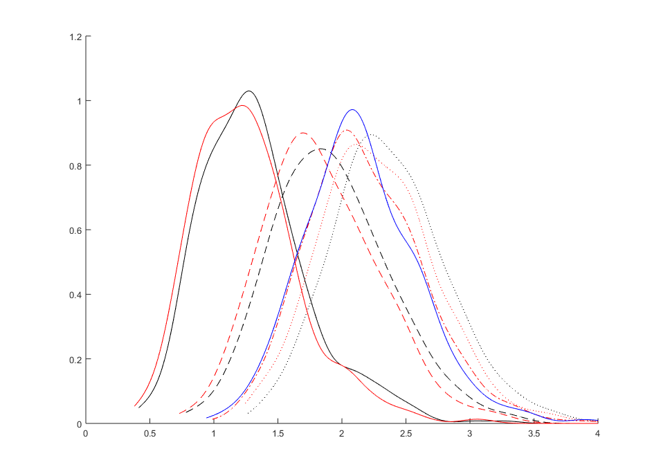
Figure 1: Density functions of the HJ statistic: (1) black solid: three strong factors; (2) black dashed: two strong factors; (3) black dotted: one strong factors; (4) blue solid: three weak proxy factors; (5) red solid: three strong factors and one useless factor; (6) red dashed: two strong factors and one useless factor; (7) red dotted: one strong factors and one useless factor; (8) red dash-dotted:one strong factors and two useless factors

The observations in Figure 1 show that values of the HJ statistic can not properly distinguish between weakly identified models and misspecified models. This is what motivates us to look further into the HJ specification test. Figure 2 compares two different approaches for approximating the distribution of the HJ statistic: one uses the conventional weighted sum of $\chi^{2}$’s, from which the critical values of the HJ statistic result, and another one uses the infeasible distribution from Theorem 2.2. The left-hand side panels of Figure 2 use three strong factors, while the right-hand side panels use three week ones.

The upper panels of Figure 2 show that both approximations for the distribution of the HJ statistic (the conventional weighted sum of $\chi^{2}(1)$s and the infeasible one from Theorem 2.2) are bad when T is small, and shift to the left compared with the density function of the HJ statistic. This observation is consistent with the one in Ahn and Gadarowski (2004) that the HJ specification test over-rejects correct model specifications in small samples. With a limited number of observation periods, not only sampling errors in the $q_{G}$ estimators need to be taken into account but also those of other estimators such as the covariance estimator $\widehat{S}$ (e.g. Kleibergen and Zhan (2020), Kleibergen et al. (2020)). The infeasible distribution improves slightly by taking into account the sampling errors in the $q_{G}$ estimators. When T is large, the randomness in the covariance estimators becomes small, but the sampling errors in $q_{G,T}$ still matter when proxy factors are weak. As shown in the lower panels of Figure 2, with a larger sample size the conventional approximation works fine when factors are strong but not when weak proxy factors are present. With weak proxy factors, the distribution of the HJ statistic is not properly approximated by the weighted sum of $\chi^{2}$’s even in large samples, and the HJ specification test is still likely to over-reject models when moment conditions do hold (Corollary 2.2.2).

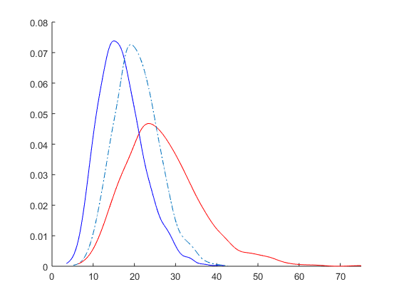
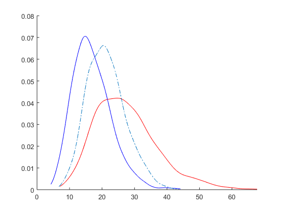
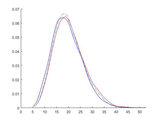
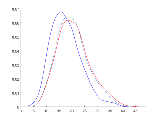
Figure 2: Density functions of the HJ statistic (red solid curve), weighted sum of $\chi^{2}$’s approximation (blue solid curves), asymptotic distribution based on Theory 2.2 (dot-dashed curve). Top left-hand side panel: $T=100,$ three strong factors $f_{t}$; top right-hand side panel: $T=100,$ three weak factors $g_{t}$; bottom left-hand side panel: $T=1000,$ three strong factors $f_{t}$; bottom right-hand side panel: $T=1000,$ three weak factors $g_{t}$.

Our second simulation exercise considers a simple single factor model in order to further illustrate the size distortion of the HJ specification test. We calibrated parameters to the data set from Kroencke (2017). We simulate the proxy factor $g_{t}\sim~{}i.i.d.~{}N(0,V_{f}/4)$, the omitted factor $v_{t}\sim~{}i.i.d.~{}N(0,Vff-d_{g}*(V_{f}/4)*d_{g}^{\prime})$, the latent factor $f_{t}=d_{g}g_{t}+v_{t}$ and thus the variance of the $f_{t}$ remain unchanged to different values of the $d_{g}$. We calibrate $V_{f}$ to match the sample variance of the consumption growth factor from the data. The factor proposed in Kroencke (2017) has been shown to be weak (e.g. Kleibergen and Zhan (2020)). Therefore, we choose $\beta$ to be of $10\widehat{\beta}$ with $\widehat{\beta}$ the sample regression parameter from Kroencke (2017), and thus $r_{t}$ is generated with one single strong factor $f_{t}$ via $r_{t}=\iota_{N}+\beta\lambda+\beta f_{t}+u_{t}$, $u_{t}\sim~{}i.i.d~{}N(0,V_{u})$, where we match $\lambda$ to the estimated risk premium from Kroencke (2017). We arbitrarily choose $d_{g}=1.9;0.9$ to mimic a strong and weak proxy factor.

Table 1 shows that the HJ specification tests have poor finite sample performances, size distortions increase with the number of assets and with relative weak proxy factors the distortion is more severe, and these observations support Corollary 2.2.2.

$\beta$	$N=5$	$N=10$	$N=15$	$N=31$
T=100, $d_{g}=1.9$	0.5032	0.8824	0.9711	0.9992
T=10000, $d_{g}=1.9$	0.1210	0.1486	0.2298	0.2238
T=100, $d_{g}=0.9$	0.7132	0.9330	0.9814	1
T=10000, $d_{g}=0.9$	0.5174	0.8906	0.8834	0.9978

Table 1: Rejection frequency table under the null (at 0.05 significance level) via the HJ specification test with critical values drawn from weighted sum of $\chi^{2}$’s

3 Specification test with limited N: HJS

As in previous discussions, the HJ specification test can not provide valid inference when weak (proxy) factors are present, and this is because the HJ specification test procedure ignores some non-negligible sampling errors in the estimates of parameters that can not be properly identified in the presence of weak identification issues. In this section, we suggest a numerically simple and identification robust test procedure which replaces the estimates of these parameters with potential identification issues by those lying in a robust confidence set. This approach is related to the widely studied weak instrument problem, where confidence sets with asymptotically correct coverage can be constructed for parameters with potential identification issues (e.g. Kleibergen (2005), Mikusheva (2010)).

3.1 HJS specification test

Our proposed HJS specification test procedure is conducted in three steps:

Step (1): Construct an identification robust confidence set, $CS_{r,\alpha_{1}}$, for $\theta_{G}$ by inverting an Anderson-Rubin (AR) type test statistic (e.g., Kleibergen (2009), Gospodinov et al. (2017)):

$$CS_{r,\alpha_{1}} =\left\{\theta\in\Theta:AR(\theta)\leq c_{1-\alpha_{1}}\right\};~{}~{}AR(\theta)=Te_{T}(\theta)^{\prime}S_{T}^{-1}({\theta})e_{T}(\theta).$$ (13)

with $c_{1-\alpha_{1}}$ the $100(1-\alpha_{1})\%$ percentile of the $\chi^{2}(N)$ distribution.

Step (2): Compute the HJS statistic:

$$\widehat{\delta}^{*}_{g}=\inf_{\theta\in CS_{r,\alpha_{1}}}\delta_{g,T}(\theta),$$ (14)

with $\delta_{g,T}=(\theta)e_{g,T}(\theta_{G})^{\prime}\widehat{Q}_{r}^{-1}e_{g,T}(\theta_{G})$. To complete the construction of the HJS statistic we set $\widehat{\delta}_{g}^{*}=\infty$ when the confidence set $CS_{r,\alpha_{1}}$ is empty.

Step (3): This test would then reject the null hypothesis that moment conditions (6) hold if

$$T\widehat{\delta}^{*}_{g}>c^{*}_{1-\alpha},$$

and the critical value is:

$$c^{*}_{1-\alpha}=\sup_{\theta\in CS_{r,\alpha_{1}}}c^{*}_{1-\alpha_{2}}(\theta),$$ (15)

where $c^{*}_{1-\alpha}(\theta)$ is the $100(1-\alpha_{1})\%$ percentile of the weighted sum of $N$ $\chi^{2}(1)$ random variables with weights being the non-zero eigenvalues of $S^{\frac{1}{2}}_{T}({\theta})\widehat{Q}_{r}^{-1}S^{\frac{1}{2}^{\prime}}_{T}({\theta})$, $\alpha_{1},$ $\alpha_{2}$ are chosen such that $\alpha_{1}>0,$ $\alpha_{2}>0$ and $\left(1-\alpha_{1}\right)\left(1-\alpha_{2}\right)=1-\alpha$ with $\alpha$ the overall significance level.

Our HJS specification test procedure combines a less powerful but robust statistic (AR) with a non-robust one (HJ) to incorporate the model identification strength in our testing procedure, and in later discussion we show that this test improves performance in size (compared with the HJ test) and power (compared with the $\mathcal{J}$ test).

Before we proceed to show the size and power performances of the HJS specification test (Theory 3.2 and Theory 3.3 ), we first discuss the properties of the robust confidence set $CS_{r,\alpha}$. Kleibergen and Zhan (2020) study a similar robust risk premia confidence set using the GRS-FAR statistic. They show that this kind of set can be unbounded in certain cases. Therefore, for practical reason, we restrict the parameter space $\Theta$ to be a compact set (Assumption 2.1), of which the robust confidence set is a subset. By construction, when the model is strongly identified we would expect the confidence set to shrink to a point as sample size grows, and when the model is weakly identified or even unidentified the diameter of this set can be arbitrarily large.

Lemma 3.1.

Suppose the assumptions in Corollary 2.2.1 hold, then

$$\lim\inf_{T}\mathbb{P}\left(\theta_{G}\in CS_{r,\alpha}\right)\geq 1-\alpha$$

Proof: See Appendix B.

Lemma 3.1 implies that the confidence set covers the true value with the requested probability asymptotically even in the presence of weak (proxy) factors, which is essential for the correct size performance of the HJS test. This result holds under more general cases, for example it holds even when the model is not identified, and this correct coverage probability of the confidence set directly results from the correct size of the identification robust AR test statistic.

Theorem 3.2.

Suppose the assumptions in Lemma 3.1 hold,

$$\lim\sup_{T}\mathbb{P}\left(T\widehat{\delta}^{*}_{g}\geq c_{1-\alpha}^{*}\right)\leq\alpha$$

Proof: See Appendix B.

Theorem 3.2 shows that $c_{1-\alpha}^{*}$ provides a upper bound for the HJS statistic, which is also a upper bound for the HJ statistic as the HJ statistic is smaller than the HJS statistic by construction, and that the HJS specification test is size correct in the presence of weak (proxy) factors. The proof of it implies that the size property of the HJS specification test is a direct result of Lemma 3.1, and given that the lemma holds for more general conditions, we know that the HJS specification test can be extended to more general cases as well. Theorem 3.2 also implies that the HJS specification test is conservative, which is understandable as we use the infimum to construct the HJS statistic instead of the supremum. However given the diameter of the robust confidence set can be arbitrarily large, using the supremum can lead to size distortion (see Example B.1).

Even though it is conservative, the HJS specification test has better power performance compared with another well-know specification test, the $\mathcal{J}$ specification test. The $\mathcal{J}$ specification test statistic is also constructed based on the AR statistic such that

$$\mathcal{J}=\inf_{\theta}AR(\theta)$$

Gospodinov et al. (2017) show that the $\mathcal{J}$ specification test is size correct in the presence of spurious/useless factors, which means $q_{G}$ is of reduced rank and the model is not identified, but it has a complete power loss in such cases. We extend their results to weakly identified models. Theory 3.3 shows that in both unidentified and weakly identified models, the $\mathcal{J}$ specification test suffers from power loss, while our HJS test still maintains proper power performance.

Theorem 3.3.

Suppose Assumptions B.1, 2.1, 2.2 hold, but instead of the correct proxy factors $g_{t}$, proxy factors $\widetilde{g}_{t}$ are used such that $\widetilde{g}_{t}$ is a $\widetilde{K}\times 1$ vector, $\left\lVert\iota_{N}-q_{\widetilde{G}}\theta_{\widetilde{G}}\right\rVert>a>0,\forall\theta_{\widetilde{G}}\in\Theta$ with $q_{\widetilde{G}}=\mathbb{E}(r_{t}\widetilde{G}_{t}^{\prime}),\widetilde{G}_{t}=(1,\widetilde{g}_{t})$ and the model is misspecified. In addition, assume that the $\psi_{B_{{g}}}$, when we replace ${G}_{t}$ with $\widetilde{G}_{t}$, in Lemma 2.1 satisfies that $\psi_{B_{{g}}}\sim N(0,Q_{\widetilde{G}}\otimes\Sigma)$ with $Q_{\widetilde{G}}=\mathbb{E}(\widetilde{G}_{t}\widetilde{G}_{t}^{\prime})$ and $\Sigma$ the covariance matrix of $\widetilde{u}_{g,t}$. Let $H=\left(\iota_{N},q_{\widetilde{G}}\right)$.

• (Gospodinov et al. (2017), Theorem 2, unidentified model under misspecification) Suppose $H$ has a column rank $K+1-k$ for an integer $k\geq 1$, then we have

  $$\mathcal{J}\preceq_{d}w_{k,i}$$

  where $w_{k,i}$ is the smallest eigenvalue of $\mathcal{W}_{k}\sim\mathcal{W}_{k}\left(N-K-1+k,I_{k}\right)$ and $\mathcal{W}_{k}\left(N-K-1+k,I_{k}\right)$ denotes the Wishart distribution with $N-K-1+k$ degrees of freedom and a scaling matrix $I_{k}$. Furthermore,

  $$\lim\sup_{T}\mathbb{P}\left(\mathcal{J}\geq c_{\chi_{N-K}^{2},1-\alpha}\right)\leq\alpha,$$

  $$\lim\inf_{T}\mathbb{P}\left(T\widehat{\delta}^{*}_{g}\geq c_{1-\alpha}^{*}\right)=1,$$

  with $c_{\chi_{N-K}^{2},1-\alpha}$ the $1-\alpha$ quantile of $\chi_{N-K}^{2}$.

• (weakly identified model under misspecification) Suppose $(HQ_{x})^{\prime}*(HQ_{x})$ with $Q_{x}=\textit{diag}(I_{K+1-k},\sqrt{T}I_{k})$ converges to a positive definite matrix, then we have

  $$\mathcal{J}\rightarrow_{d}w_{k,ii}$$

  where $w_{k,ii}$ is the smallest eigenvalue of $\mathcal{W}_{k}\sim\mathcal{W}_{k}\left(\mu,N-K-1+k,I_{k}\right)$ and $\mathcal{W}_{k}\left(\mu,N-K-1+k,I_{k}\right)$ denotes the non-central Wishart distribution with $N-K-1+k$ degrees of freedom and a scaling matrix $I_{k}$, a location parameter $\mu$ ($\mu$ is specified in the proof). Furthermore,

  $$\lim\inf_{T}\mathbb{P}\left(\mathcal{J}\geq c_{\chi_{N-K}^{2},1-\alpha}\right)<1,$$

  $$\lim\inf_{T}\mathbb{P}\left(T\widehat{\delta}^{*}_{g}\geq c_{1-\alpha}^{*}\right)=1,$$

  with $c_{\chi_{N-K}^{2},1-\alpha}$ the $1-\alpha$ quantile of $\chi_{N-K}^{2}$.

Proof: See Appendix B.

3.2 Simulation exercises

In this section, we conduct a simple simulation exercise with a single-factor model to evaluate the empirical rejection rates (the size and power performance) of our proposed HJS specification test. We calibrate the data generating process in our simulations to match the data set from Kroencke (2017). We simulate the factor $f_{t}\sim~{}i.i.d.~{}N(0,V_{f})$, where we set $V_{f}$ to match the sample variance of the consumption growth factor. $r_{t}$ is generated with one factor $f_{t}$ via $r_{t}=\iota_{N}+\beta\lambda+\beta_{\perp}d+\beta d_{g}f_{t}+u_{t}$, $u_{t}\sim~{}i.i.d~{}N(0,V_{u})$, where we match $\lambda$ to the estimated risk premium, $\beta$ is the sample slope parameter between the assets returns and consumption growth factor, and $V_{u}$ is the sample covariance of the residuals resulting from regressing asset returns on a constant and the consumption growth factor. $\beta_{\perp}$ is a vector which is orthogonal to $\iota_{N},\beta$ and $\left\lVert\sqrt{T}\beta_{\perp}\right\rVert=1$. We set $T=100$. We use $d_{g}$ to tune the identification strength of the factors in our simulation exercise where a larger $d_{g}$ means a stronger factor, and $d$ to tune the model misspecification level where a lager $d$ means a larger deviation from the moment conditions (6) for our simulated data.

For the size performance comparison, we set $d=0$ and thus moment conditions (6) hold for our simulated data. Figure 3 shows that the HJ specification test is highly size distorted and the distortion only drops down slightly when we increase the identification strength of the factor, while the HJS specification test has a better finite sample behavior and remains size correct.

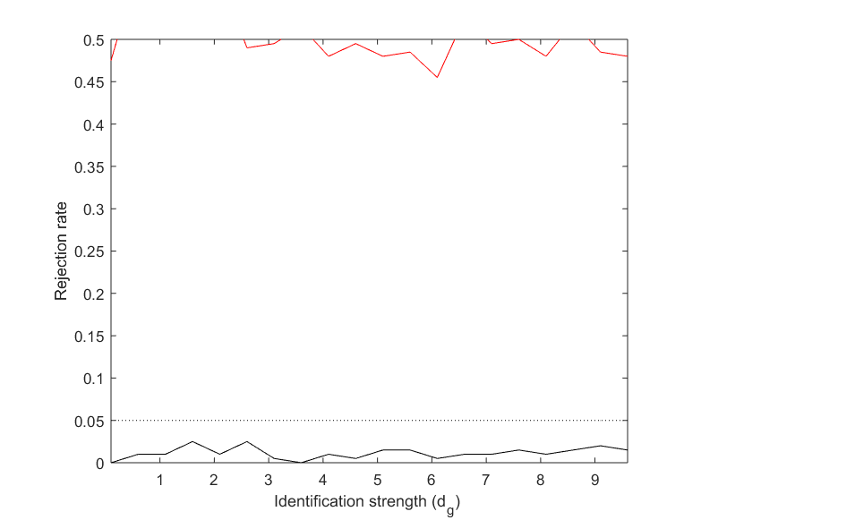
Figure 3: Size against strength of the factor ($d_{g}$): rejection frequency of the HJ specification test (red) and rejection frequency of the HJS specification test (black)

For the power performance comparison, we set $d_{g}=0$ which means $f_{t}$ only serves as a spurious factor. Figure 4 shows that the rejection frequency of the HJS specification test increases much faster compared with the one of the $\mathcal{J}$ specification test when the level of model misspecification ($d$) increases. The rejection frequency of the $\mathcal{J}$ specification test remains relatively small even when the HJS specification test rejection frequency is close to one, and this implies the HJS specification test has better power performance.

These observations support our theory and show that the HJS specification test has good performance in both size and power.

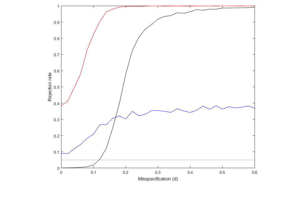
Figure 4: Power against the level of the model misspecificaion ($d$) with single spurious factor ($d_{g}=0$): rejection frequency of the HJ specification test (red), rejection frequency of the HJS specification test (black) and rejection frequency of the $\mathcal{J}$ specification test (blue)

4 Specification testing with large N: HJN

In the previous section, we construct the HJS statistic using a robust confidence set of $\theta_{G}$ since it is only weakly identified with a limited number of asset returns. The HJS specification testing procedure involves optimization steps, which is commonly done in practice through a grid search procedure. In this section, we provide another novel valid specification test statistic, the HJN statistic, which does not involve any time consuming optimization procedure. The construction of the HJN statistic uses a consistent $\theta_{G}$ estimator, and thus we first introduce our $\theta_{G}$ estimator and then the HJN statistic.

4.1 Four-pass estimator

When we work within a double-asymptotic framework such that both the number of time periods and the number of asset returns grow, weak (proxy) factors do not necessarily lead to a weak identification problem (Anatolyev and Mikusheva (2018)), which is similar to the case of many weak instruments that information about some parameters though limited, aggregates slowly. Even though $\widehat{\theta}_{G}$ is not consistent (Theory B.2), another consistent estimator for $\theta_{G}$ can be constructed. With an extended number of asset returns, we can estimate $\theta_{G}$ consistently by removing the missing factor structure via PCA and using an IV-type technique to correct for the remaining issues. The consistent estimator gives another way to construct a statistic for the HJ distance, based on which we propose a novel specification test statistic, our HJN statistic. In the following, we first introduce our four-pass $\theta_{G}$ estimator with the extended number of asset returns, and thereafter provide the motivation for this four-pass procedure.

We propose the following steps to estimate $\theta_{G}$ with $N$ base portfolios of gross returns $r_{t}$:

Step (1): Estimate $\widehat{c},\widehat{\beta}_{g}$ in the linear observed-(proxy)-factor model (4) via OLS with $N$ base portfolios of returns.

Step (2): Determine the omitted factor structure using the following two steps:

(2.1) Determine the number of factors, $K_{vz}$, in $\widehat{u}_{g,t}=r_{t}-\widehat{c}-\widehat{\beta}_{g}\bar{g}_{t}$ by

$$\widehat{K}_{vz}=\arg\min_{0\leq j\leq K_{vz,\max}}\left(N^{-1}T^{-1}\lambda_{j}\left(\widehat{u}_{g}\widehat{u}_{g}^{\prime}\right)+j\phi(N,T)\right)-1$$

where $\lambda_{j}(A)$ is the $j$-th largest eigenvalue of a given matrix $A$, $\widehat{u}_{g}$ is $T\times N$ matrix stacked with the OLS residuals $\widehat{u}_{g,t}$, $K_{vz,\max}$ is an arbitrary upper bound for $K_{vz}$ and $\phi(N,T)$ is a penalty function with the properties $\phi(N,T)\rightarrow 0,\phi(N,T)/(N^{-\frac{1}{2}}+T^{-\frac{1}{2}})\rightarrow\infty$ (e.g., in later simulation exercise and empirical application we simply choose $\phi(N,T)=N^{-\frac{1}{4}}+T^{-\frac{1}{4}}$);

(2.2): Estimate the $T\times N$ common component matrix ${cc}={x}{b}^{\prime}$ stacked with the common components $cc_{t}$, $\widetilde{cc}=\widehat{x}\widehat{b}$, such that $\widehat{x}$ is equal to $\sqrt{T}$ times the eigenvector associated with the $\widehat{K}_{vz}$ largest eigenvalues of the matrix $\widehat{u}_{g}\widehat{u}_{g}^{\prime}$, and $\widehat{b}=\widehat{x}^{\prime}\widehat{u}_{g}/T$ corresponds with the OLS estimator regressing $\widehat{u}_{g}$ on $\widehat{x}$:

$$\left(\widehat{x},\widehat{b}\right)=\arg\min_{b_{i},x_{t}~{}s.t.~{}\sum_{t=1}^{T}x_{t}x_{t}^{\prime}/T=I_{\widehat{K}_{vz}}}\sum_{i,t}\left(\widehat{u}_{g,it}-b_{i}^{\prime}x_{t}\right)^{2}$$

Step (3): Split the sample into two non-overlapping subsamples along the time index and remove the missing factor structure from the regressors in the SDF of both subsamples:

$$\widetilde{q}_{G,T}^{(i)}=q_{G,T}^{(i)}-\widetilde{cc}_{G,T}^{(i)^{\prime}},i=1,2$$

where

$$q_{G,T}^{(1)}=\frac{1}{\lfloor\frac{T}{2}\rfloor}\sum_{t=1}^{\lfloor\frac{T}{2}\rfloor}r_{t}G_{t}^{\prime};~{}q_{G,T}^{(1)}=\frac{1}{T-\lfloor\frac{T}{2}\rfloor}\sum_{t=\lfloor\frac{T}{2}\rfloor+1}^{T}r_{t}G_{t}^{\prime}$$

$$\widetilde{cc}_{G,T}^{(2)}=\frac{1}{\lfloor\frac{T}{2}\rfloor}\sum_{t=1}^{\lfloor\frac{T}{2}\rfloor}\widetilde{cc}_{t}G_{t}^{\prime};~{}\widetilde{cc}_{G,T}^{(2)}=\frac{1}{T-\lfloor\frac{T}{2}\rfloor}\sum_{t=\lfloor\frac{T}{2}\rfloor+1}^{T}\widetilde{cc}_{t}G_{t}^{\prime}.$$

Step (4): We then use IV regression to derive two estimators, $\widetilde{\theta}_{G}^{(i)},i=1,2$, where we use $\widetilde{q}_{G,T}^{(1)}$ as instrument for $\widetilde{q}_{G,T}^{(2)}$ and vice versa. Thereafter, our proposed four-pass estimator is derived by taking the average of both estimators:

$$\widetilde{\theta}_{G}=\sum_{i=1}^{2}\widetilde{\theta}_{G}^{(i)}/2,$$

with $\widetilde{\theta}_{G}^{(1)}=\left(\widetilde{q}^{(1)^{\prime}}_{G,T}P_{\widetilde{q}^{(2)}_{G,T}}\widetilde{q}^{(1)}_{G,T}\right)^{-1}\widetilde{q}^{(1)^{\prime}}_{G,T}P_{\widetilde{q}^{(2)}_{G,T}}\iota_{N}$ and $\widetilde{\theta}_{G}^{(2)}=\left(\widetilde{q}^{(2)^{\prime}}_{G,T}P_{\widetilde{q}^{(1)}_{G,T}}\widetilde{q}^{(2)}_{G,T}\right)^{-1}\widetilde{q}^{(2)^{\prime}}_{G,T}P_{\widetilde{q}^{(1)}_{G,T}}\iota_{N}$.

Our estimation approach for $\theta_{G}$ resolves the problems of the missing factor structure and the weak (proxy) factors simultaneously. We make use of the results from Bai and Ng (2002), Bai (2003) and Giglio and Xiu (2017) in step (2) to recover the common components in the error terms using principal component analysis, and we use the instrumental variable idea applied for the factor models, which is used in Anatolyev and Mikusheva (2018), in step (4) to solve potential endogeneity issues. Compared with the estimator proposed in Anatolyev and Mikusheva (2018), our proposed estimator relaxes the restrictions on the number of omitted factors and the restrictions on the rank of the loadings of all the factors present in the model.

To illustrate why our proposed procedure is robust against weak (proxy) factors and a missing factor structure, we start by comparing it with the conventional $\theta_{G}$ estimator. To do so, we first rewrite equation (6) ($\iota_{N}=\mathbb{E}q_{G,T}\theta_{G}$) as

$$\iota_{N}={q}_{G,T}{\theta}_{G}-\epsilon_{q_{G}}{\theta}_{G},$$

with $\epsilon_{q_{G}}=\left({q}_{G,T}-\mathbb{E}{q}_{G,T}\right)$ which is correlated with $q_{G,T}$. The term $\epsilon_{q_{G}}$ vanishes asymptotically, and so it is dominated by $q_{G,T}$ when all proxy factors are strong. The conventional estimator, which results from regressing $\iota_{N}$ on $q_{G,T}$, is then valid in large samples, since $\epsilon_{q_{G}}$ becomes negligible. However, if some (proxy) factors are weak, some columns of $q_{G,t}$ are of the same order as $\epsilon_{q_{G}}$, then there would be a classic endogeneity problem if we simply regress $\iota_{N}$ on ${q}_{G,T}$.

To solve the endogeneity problem, a valid instrument can be constructed in our framework with a split-sample technique and this idea is also employed in Anatolyev and Mikusheva (2018). Given the independence of the $e_{t}$ from non-overlapping sub-samples, $q_{G,T}^{(1)}$ can serve as an instrument for $q_{G,T}^{(2)}$ and vice versa when there is no missing factor structure ($K_{vz}=0$) and this is the starting point of our proposed procedure. When there is a missing factor structure with factors that might be correlated across time, $q_{G,T}^{(1)}$ is no longer a valid instrument for $q_{G,T}^{(2)}$. Therefore, we use $\widetilde{q}_{G,T}^{(i)},i=1,2$ which results from removing the missing factor structure from $q_{G,T}^{(i)},i=1,2$. By doing so, $\widetilde{q}_{G,T}^{(1)}$ is asymptotically uncorrelated with $\widetilde{\epsilon}_{q_{G}}^{(2)}$, and is a valid instrument.

As shown in Theorem 4.1, our estimation procedure provides $\min\{\sqrt{T},\sqrt{N}\}$-consistent results for $\theta_{G}$, of which a non-linear transformation leads to a consistent risk premia estimator (Corollary 4.1).

Theorem 4.1.

Suppose Assumptions 2.1 - 2.3, C.1 - C.9 hold, and $N/T\rightarrow c$.

$$\sqrt{NT}Q^{-1}_{B_{g},T}\left(\widetilde{\theta}_{G}-\theta_{G}\right)\rightarrow O_{p}(1),$$

with $Q_{B_{g},T}=\text{diag}(I_{1+K_{g,1}},\sqrt{T}I_{1+K_{g,1}})$.

Proof: See Appendix C .

Corollary 4.1.1.

Suppose the assumptions in Theorem 4.1 hold, then

$$\sqrt{NT}Q^{-1}_{x}\left(\widetilde{\lambda}_{g}-\lambda_{g}\right)\rightarrow O_{p}(1),$$

with $\widetilde{\lambda}_{g}=-V_{g}\text{diag}(0_{K\times 1},I_{K})\widetilde{\theta}_{G}/\widetilde{\theta}_{G,1}$.

Proof: This is a direct result of Theorem 4.1.

4.2 HJN specification test

Kleibergen and Zhan (2018) study risk premia on mimicking portfolios by projecting non-traded factors on traded base portfolios, and then carry out identification robust tests using a set of testing portfolios. We use a similar idea to construct the HJN specification test:
Step (1) Estimate $\theta_{G}$ from a set of N base portfolios $r_{t}$ of asset returns using our proposed four-pass estimator $\widetilde{\theta}_{G}$

Step (2) Estimate $q_{G}$ from a set of testing portfolios $R_{t}$ of n asset returns and $n$ is fixed such that $\widetilde{q}_{G}=\frac{1}{T}\sum_{t=1}^{T}R_{t}G_{t}^{\prime}$

Step (3) The HJN statistic is

$$\widetilde{\delta}_{g}^{2}=\widetilde{e}_{T}^{\prime}\widehat{Q}_{R}^{-1}\widetilde{e}_{T},$$

with sample pricing errors $\widetilde{e}_{T}=\iota_{n}-\widetilde{q}_{G}\widetilde{\theta}_{G}$, $\widehat{Q}_{R}=\frac{1}{T}\sum_{t=1}^{T}R_{t}R_{t}^{\prime}$.

Step (4) This test would reject the null hypothesis that moment conditions (6) hold if

$$T\widetilde{\delta}_{g}>\widetilde{c}_{1-\alpha},$$

where $\widetilde{c}_{1-\alpha}$ is the $1-\alpha$ quantile of the weighted sum of $N$ $\chi^{2}(1)$ random variables with weights being the positive eigenvalues of the matrix $\widetilde{S}^{\frac{1}{2}}(\widehat{Q}_{R})^{-1}\widetilde{S}^{\frac{1}{2}^{\prime}}$ with $\widetilde{S}$ a consistent estimator of the long-run variance matrix of the sample pricing errors ${e}_{T,R}(\theta_{G})=\iota_{n}-\widetilde{q}_{G}{\theta}_{G}$.

Remark: the HJN specification test does not require the base portfolios and testing portfolios to be non-overlapping.

Corollary 4.1.2.

Suppose the assumptions in Theorem 4.1 hold, then

$$T\widetilde{\delta}_{g}^{2}\sim_{d}\sum_{i=1}^{n}{p}_{i}x_{i}$$

with $x_{i}$ being independently $\chi^{2}(1)$ distributed random variables and $p_{i}$ being the positive eigenvalues of the matrix $\widetilde{S}^{\frac{1}{2}}(\widehat{Q}_{R})^{-1}\widetilde{S}^{\frac{1}{2}^{\prime}}$ with $\widetilde{S}$ a consistent estimator of the long-run variance matrix of the sample pricing errors ${e}_{T,R}(\theta_{G})$ (for example, one may simple choose $\widetilde{S}=\frac{1}{T}\sum_{t=1}^{T}e_{g,t,R}(\widetilde{\theta}_{G})e_{g,t,R}(\widetilde{\theta}_{G})^{\prime},e_{g,t,R}({\theta}_{g})=\iota_{N}-R_{t}G_{t}^{\prime}{\theta}_{g}$).

Proof: See Appendix C.

Theorem 4.2 shows that our HJN specification test is size correct even with weak (proxy) factors.

Theorem 4.2.

Suppose the assumptions in Theorem 4.1 hold,

$$\lim\sup_{T}\mathbb{P}\left(T\widetilde{\delta}_{g}\geq\widetilde{c}_{1-\alpha}\right)=\alpha$$

with $\widetilde{c}_{1-\alpha}$ the $1-\alpha$ quantile of the weighted sum of $N$ $\chi^{2}(1)$ random variables with being the positive eigenvalues of the matrix $\widetilde{S}^{\frac{1}{2}}(\widehat{Q}_{R})^{-1}\widetilde{S}^{\frac{1}{2}^{\prime}}$ with $\widetilde{S}$ a consistent estimator of the long-run variance matrix of the sample pricing errors ${e}_{T,R}(\theta_{G})$ (for example, one may simple choose $\widetilde{S}=\frac{1}{T}\sum_{t=1}^{T}e_{g,t,R}(\widetilde{\theta}_{G})e_{g,t,R}(\widetilde{\theta}_{G})^{\prime},e_{g,t,R}({\theta}_{g})=\iota_{N}-R_{t}G_{t}^{\prime}{\theta}_{g}$).

Proof: This is a direct result from Corollary 4.1.2.

4.3 Simulation exercise and empirical application

Similar to section 3.2, we again evaluate the empirical rejection rates of our HJS specification test via simulation exercises.

We calibrate to the data set used in Anatolyev and Mikusheva (2018): the monthly returns on 100 Fama-French portfolios sorted by size and book-to-market and three Fama-French factors ($g_{t}$). From the portfolio returns we obtain the first four principal components (PC), and we regard the first three PCs as priced latent common factors, $f_{t}$, and the fourth one as the omitted factor, $z_{t}$. With normalization $\left(f,z\right)^{\prime}\left(f,z\right)/T=I_{4}$, we set the variance of these factors to be $1$. We regress demeaned returns on $f_{t},z_{t}$ for their risk exposures, and calculate the sample mean $\mu_{\beta\gamma}$ and the sample variance $V_{\beta\gamma}$ of the risk exposures. We compute the sample variance $\sigma_{e}^{2}I_{N}$ of the residuals after regressing returns on $f_{t},z_{t}$. To maintain the relation between observed factors $g_{t}$ and PCs $f_{t}$, we regress $f_{t}$ on the three Fama French factors to obtain the slope $d_{g}$ and residual covariance matrix $V_{v}$, and $d_{g}$ captures the quality of the proxy factors.

We then simulate our data in the following way. In the first step we simulate observed factors from i.i.d $N(0,I_{3})$ and latent factors $f_{t}$ are generated by $Ad_{g}g_{t}+v_{t}$ with $v_{t}$ simulated as i.i.d $N\left(0,(I-A)d_{g}d_{g}^{\prime}(I-A)+V_{v}\right)$. $A$ is a diagonal matrix which we use to adjust the strengths of our (proxy) factors, and we set $A=\text{diag}(I_{2},d_{\alpha})$ in our simulations with $d_{\alpha}$ tuning the strength of the simulated factors. As for the corresponding risk exposures, we use $(\beta_{i}^{\prime},\gamma_{i}^{\prime})^{\prime}\sim$ i.i.d $N(\mu_{\beta\gamma},V_{\beta\gamma})$. Then in the end, we generate $r_{t}=\iota_{N}+\beta_{\perp}d+\beta\lambda+\beta f_{t}+\gamma z_{t}+e_{t}$, $e_{t}\sim~{}i.i.d~{}N(0,\sigma_{e}^{2}I_{N})$, where we match $\lambda$ to the estimated risk premia resulting from the data. $\beta_{\perp}$ is a vector which is orthogonal to $\iota_{N},\beta$ and $\left\lVert\beta_{\perp}\right\rVert=1$. Similar to the previous simulation setting in Figure 4 we use $d$ to tune the model misspecification level and $d=0$ when we simulate size curves.

In our simulations, we fix $N=100$. For the HJN specification test we use all the simulate 100 asset gross returns to form the base portfolios and the first 25 to form the testing portfolios, and we use the testing portfolios for the conventional HJ specification test.

Figure 5 compares the size curves of the HJ specification test and of the HJN specification test. It shows that the HJ specification test is highly size distorted even when $d_{\alpha}$ is large (left hand side panel of Figure 5) and the size distortion increases when proxy factors become weaker (smaller $d_{\alpha}$), while the HJN specification test roughly remains size correct. Even with relatively large number of time periods, the conventional HJ specification test still over-reject. Observations from Figure 5 also seem to imply that our HJN specification test tends to under-reject in finite samples, and to show it performs well when the model is misspecified we also simulate power curves in Figure 6.

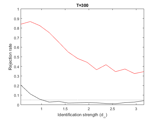
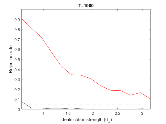
Figure 5: Size against strength of the factor ($d_{\alpha}$): rejection frequency of the HJ specification test (red) and rejection frequency of the HJN specification test (black). Left hand side panel: T=300; right hand side panel: T=1000

Figure 6 shows power curves of the HJ specification test and the HJN specification test respectively. The left hand side panel of Figure 6 uses $d_{\alpha}=0.5$ to mimic one weak proxy factor, while all proxy factors in the right hand side panel are strong with a larger value of $d_{\alpha}$. Figure 6 shows that the HJN specification test has proper power performance regardless of the presence of weak (proxy) factors, and rejection frequency increases faster when the proxy factor is stronger.

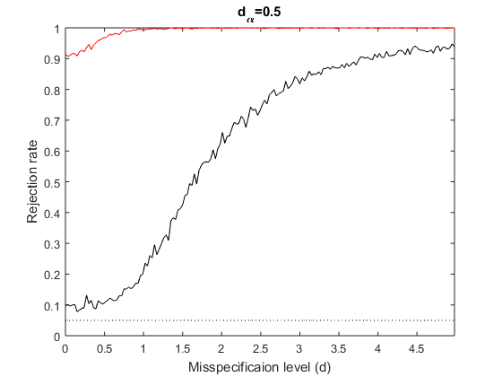
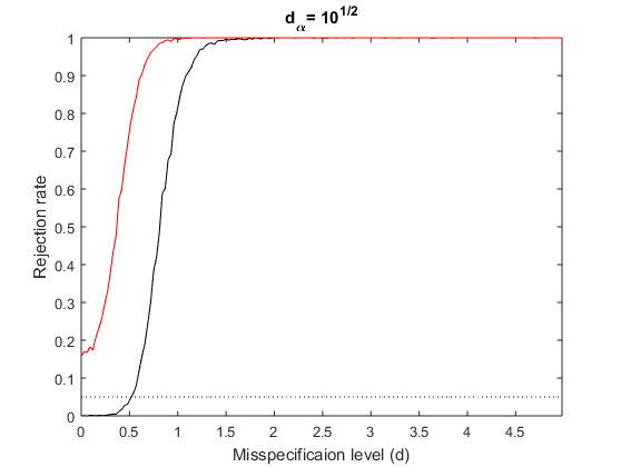
Figure 6: Power against the level of the model misspecificaion ($d$): rejection frequency of the HJ specification test (red) and rejection frequency of the HJS specification test (black). Left hand side panel: with one weak proxy factor $d_{\alpha}=0.5$; Right hand side panel: with strong factors $d_{\alpha}=\sqrt{10}$.

5 Empirical application

We apply our proposed test procedures on the data set of monthly returns on 100 Fama-French portfolios sorted by size and book-to-market and the three Fama-French factors (market, SmB, HmL) and the momentum factor.

An intuitive measure for the factor structure in asset returns is total variation of the asset returns explained by the principal components (Kleibergen and Zhan (2015)). We construct the spectral decomposition of the sample covariance matrix of the 100 portfolio returns, and denote $\lambda_{1}>\lambda_{2}>\cdots$ the characteristic roots (or eigenvalues of the PCs of asset returns) in descending order. We use the characteristic roots ratios (CRRs) ${\lambda_{i}}/{\left(\sum_{j}\lambda_{j}\right)},i=1,2,3,4$, which represent the total variation of the portfolio returns explained by the first four PCs respectively, to check the factor structure of portfolio returns (see Figures 7 and 9).

Figures 7 and 9 also report the p-values of specification tests (HJ and HJN) with respect to a three-FF-factor model and a four-factor (adding the momentum) model from 1963-09 to 2019-08 using rolling windows of 240 and 120 months respectively. For the HJN specification test we use all the 100 asset returns to form the base portfolios and the first 25 to form the testing portfolios, and we use the testing portfolios for the conventional HJ specification test. They also report measures for the presence of a factor structure in the asset returns: the fraction of the total variation of the portfolio returns that is explained by their principal components.

Figures 7 shows that when comparing nested models, the HJ test can produce counter-intuitive results by rejecting a four-factor model but not the reduced three-factor model (see points near the coordinate ’2015-01’). This is an unfortunate outcome since the four-factor mode apparently embeds the three-factor model and if the four-factor model is rejected we would expect the three-factor model to be rejected as well. We attribute this strange behavior to the momentum factor having only weak correlation with the returns and thus inducing a larger rejection rate of the HJ test, while our HJN specification test does not have such problem.

The HJN specification test also captures changes in the factor structure of asset returns in a more sensible way compared with the HJ test. As shown in Figure 7, when CRRs vary in different time periods (e.g., the total variation of the portfolio returns is mostly explained by the first PC for points near the coordinate ’2000-01’ while the other PCs only account for a much lower percentage of the variation), the HJN specification tests reflect the changes in the factor structure of asset returns with variations in p-values of tests of a four-factor model, while the HJ specification tests reject both three-factor and four-factor models for most time periods and is not informative for the factor structure of asset returns.

Both of the HJ and the HJN tests in Figure 7 seem to have larger p values near the coordinate ’2015-01’ while the patterns of characteristic roots ((a) and (b)) seem to be rather stable. This is because a 240-month window size is a bit too long, and some changes in the factor structure might be averaged out and thus not detected by CRRs. We choose a smaller rolling window size (120 months) in Figure 9, and it shows the change in the factor structure (Figure 9.(a)) after the coordinate ’2010-01’. Similar to what we observe in Figure 7, Figure 9 also shows our HJN specification test respond to the factor structure in the asset returns in a more informative way, while the HJ tests only report small p values for most time periods for both three- and four-factor models.

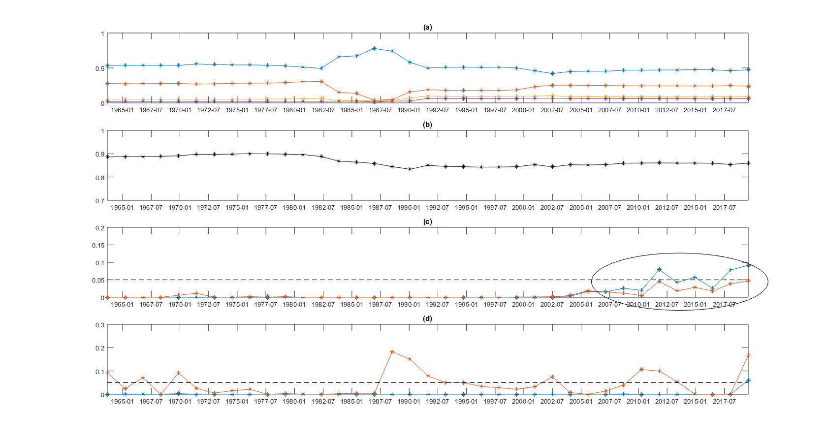
Figure 7: The time series of estimates from 1963-09 to 2019-08 with rolling windows of size T = 240 (20 years) and the number of increments between successive rolling windows being 12 (1 year) (x-axis is labeled with the ending period of each rolling window, for example, the first rolling window uses data from 1963-09 to 1983-08, so x-axis should label the first point with ’1983-08’). (a) The fraction of the total variation of the portfolio returns that is explained by their four largest principal components respectively (CRRs) ($\lambda_{i}/(\sum_{j=1}^{N}\lambda_{j}),i=1,\cdots,4$); (b) The fraction of the total variation of the portfolio returns that is explained by the sum of the four largest principal components ($\sum_{i=1}^{4}\lambda_{i}/(\sum_{j=1}^{N}\lambda_{j})$); (c) p-values of the HJ specification test of the three-FF-factor model (blue), p-values of the HJ specification test of the four-factor (three FF and momentum factors) model (red);(d) p-values of the HJN specification test of the three-FF-factor model (blue), p-values of the HJN specification test of the four-factor model (red).

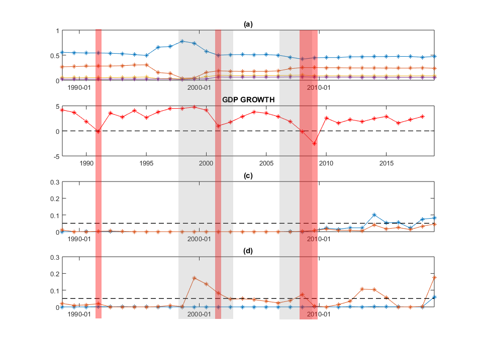
Figure 8: The time series of estimates from 1968-09 to 2019-08 with rolling windows of size T = 240 (20 years) and the number of increments between successive rolling windows being 12 (1 year) (x-axis is labeled with the ending period of each rolling window, for example, the first rolling window uses data from 1968-09 to 1988-08, so x-axis should label the first point with ’1988-08’). (a) The fraction of the total variation of the portfolio returns that is explained by their four largest principal components respectively (CRRs) ($\lambda_{i}/(\sum_{j=1}^{N}\lambda_{j}),i=1,\cdots,4$); (b) (GDP growth) US GDP annual growth rate 1988-2018 (downloaded from the World Bank); (c) p-values of the HJ specification test of the three-FF-factor model (blue), p-values of the HJ specification test of the four-factor (three FF and momentum factors) model (red);(d) p-values of the HJN specification test of the three-FF-factor model (blue), p-values of the HJN specification test of the four-factor model (red).

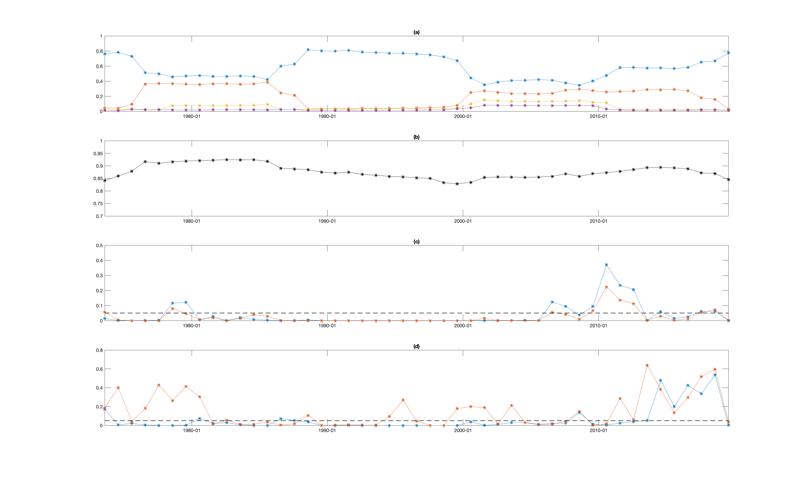
Figure 9: The time series of estimates from 1963-09 to 2019-08 with rolling windows of size T = 240 (20 years) and the number of increments between successive rolling windows being 12 (1 year) (x-axis is labeled with the ending period of each rolling window). (a) The fraction of the total variation of the portfolio returns that is explained by their four largest principal components respectively (CRRs) ($\lambda_{i}/(\sum_{j=1}^{N}\lambda_{j}),i=1,\cdots,4$); (b) The fraction of the total variation of the portfolio returns that is explained by the sum of the four largest principal components ($\sum_{i=1}^{4}\lambda_{i}/(\sum_{j=1}^{N}\lambda_{j})$); (c) p-values of the HJ specification test of the three-FF-factor model (blue), p-values of the HJ specification test of the four-factor (three FF and momentum factors) model (red);(d) p-values of the HJN specification test of the three-FF-factor model (blue), p-values of the HJN specification test of the four-factor model (red).

We observe in Figures 7 and 9 that the HJN specification tests in some rolling windows do not reject a four-factor model. To further study this observation, Table 2 reports results based on the data from 1977-08 to 2019-08. We see in Table 2 that both the HJ and HJN specification tests reject the three-factor model, and while the HJ specification test rejects the four-factor model, the HJN specification test does not reject it. Our HJS specification test seems to be a bit conservative and does not reject both models in this application. The estimates for the four-factor model using our proposed approach indicate a larger change in values corresponding to the momentum factor, and this might result from the momentum factor being weak. Our specification tests support a four-factor model for Fama French portfolios, and observations show that the momentum factor might only serve as a weak proxy factor which can explain the difference between the HJ and the HJN specification test results and the differences in estimated parameter values.

	HJ(p-val)	HJN(p-val)	HJS(rejected)
n=25
Three factor	0.000	0.000	No
Four factor	0.000	0.0694	No

Table 2: Tests of specification using monthly returns on 100 portfolios sorted by size and book-to-market and the three Fama-French factors and the momentum factor from 1977-08 to 2019-08

6 Conclusions

We show that the HJ statistic is not a valid model selection tool and model specification test statistic when weak (proxy) factors are present. We propose two novel approaches that provide size-correct model specification tests, alongside with which we also propose novel weak (proxy) factors robust risk premia estimators. Our empirical application supports a four factor structure for Fama French portfolios despite that the momentum factor is a weak proxy factor.

Appendix A Additional figures and tables

This section provides additional figures and tables. Mainly, we provide more results for our empirical application in Section 5, and further illustrate how the conventional tests may fail in some empirically relevant settings.

Figure 10 illustrates the density function of the HJS statistic under same settings as in Figure 1. We use our previous simulation experiment calibrated to data from Lettau and Ludvigson (2001) to illustrate properties of the HJS statistic. The black dotted curve in Figure 10 suggests the value of the HJS statistic could be small when the model is not correctly specified. These smaller values are due to much smaller confidence sets $CS_{r}$ when model is not correctly specified. Therefore, using the HJS statistic as a model selection tool may not be a good idea even though it provides size correct specification test.

Figures 11 and 12 follow the same settings as in Figures 7 and 9, and they provide additional results by adding the p-values of the rank test (Kleibergen and Paap (2006)) of $q_{G}$ (the rank of $q_{G}$ reflects the identification strength of the model, e.g., Kleibergen and Zhan (2020), Kleibergen et al. (2020), as it shows whether the sample pricing errors vary enough as a function of $\theta$), and the p-values of the $\mathcal{J}$ specification test.

Figures 11 and 12 show that the $\mathcal{J}$ specification tests tend to give larger p-values, and thus it is less informative. When we use 10-year window size (Figure 12) instead of the 20-year window size (Figure 11), the p-values of the rank test increase and the lack of identification strength also increases the p-values of the $\mathcal{J}$ test. For points near the coordinate ’1990-01’ in Figure 12, the rank test can not reject that the $q_{G}$ is of reduced rank (lack of identification strength), and the corresponding $\mathcal{J}$-test p-values increase while the HJ tests tend to have larger p-values for testing the reduced three-factor model than the four-factor model. In short, in the presence of weak (proxy) factors, both well-know test statistics can not provide satisfying inference results.

Tables 4 and 3 follow the same settings as in Table 2 and reports additional results: tests with different value of n and parameter estimates. If n is getting too large, the HJN test also suffers from finite sample issues and tends to have smaller p-values, as its validity requires $n/N\rightarrow 0$. We leave the construction of a high-dimensional robust test statistic for further study.

	HJ(p-val)	HJN(p-val)	HJS(rejected)
n=30
Three factor	0.000	0.000	No
Four factor	0.000	0.054	No
n=35
Three factor	0.000	0.000	No
Four factor	0.000	0.027	No
n=40
Three factor	0.000	0.000	No
Four factor	0.000	0.026	No

Table 3: Tests of specification using monthly returns on 100 portfolios sorted by size and book-to-market and the three Fama-French factors and the momentum factor from 1977-08 to 2019-08

	Market	SMB	HML	MOM
(1)
$\widehat{\theta}_{G}$	0.0480	-0.0013	-0.0127	$-$
$\widetilde{\theta}_{G}$	0.3081	-0.1296	0.1370	$-$
$\widehat{\lambda}_{g}$	-5.2108	0.4037	-0.0347	$-$
$\widetilde{\lambda}_{g}$	-5.4740	0.3250	-0.2261	$-$
(2)
$\widehat{\theta}_{G}$	0.0472	0.0174	-0.0172	0.0240
$\widetilde{\theta}_{G}$	0.1146	-0.4108	0.2233	-0.8945
$\widehat{\lambda}_{g}$	-3.7893	0.6822	-0.3995	1.5882
$\widetilde{\lambda}_{g}$	-2.8368	0.9104	-0.6567	3.6223

Table 4: Estimates with Fama-French factors and the momentum factor using monthly returns on 100 portfolios sorted by size and book-to-market from 1977-08 to 2019-08

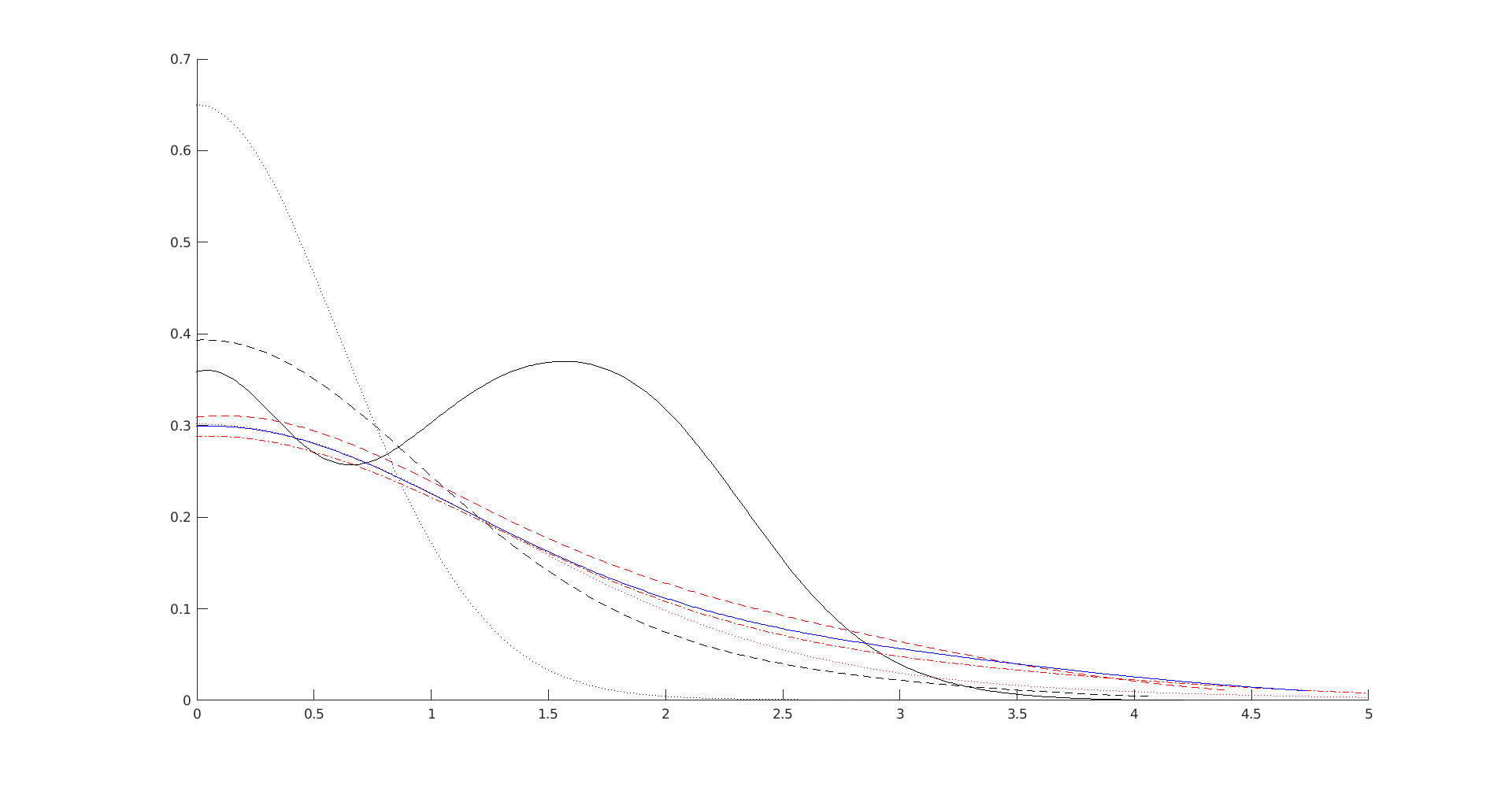
Figure 10: Densities of the HJS statistic: (1) black solid: three strong factors; (2) black dashed: two strong factors; (3) black dotted: one strong factors; (4) blue solid: three weak proxy factors; (5) red solid: three strong factors and one useless factor; (6) red dashed: two strong factors and one useless factor; (7) red dotted: one strong factors and one useless factor; (8) red dash-dotted:one strong factors and two useless factors

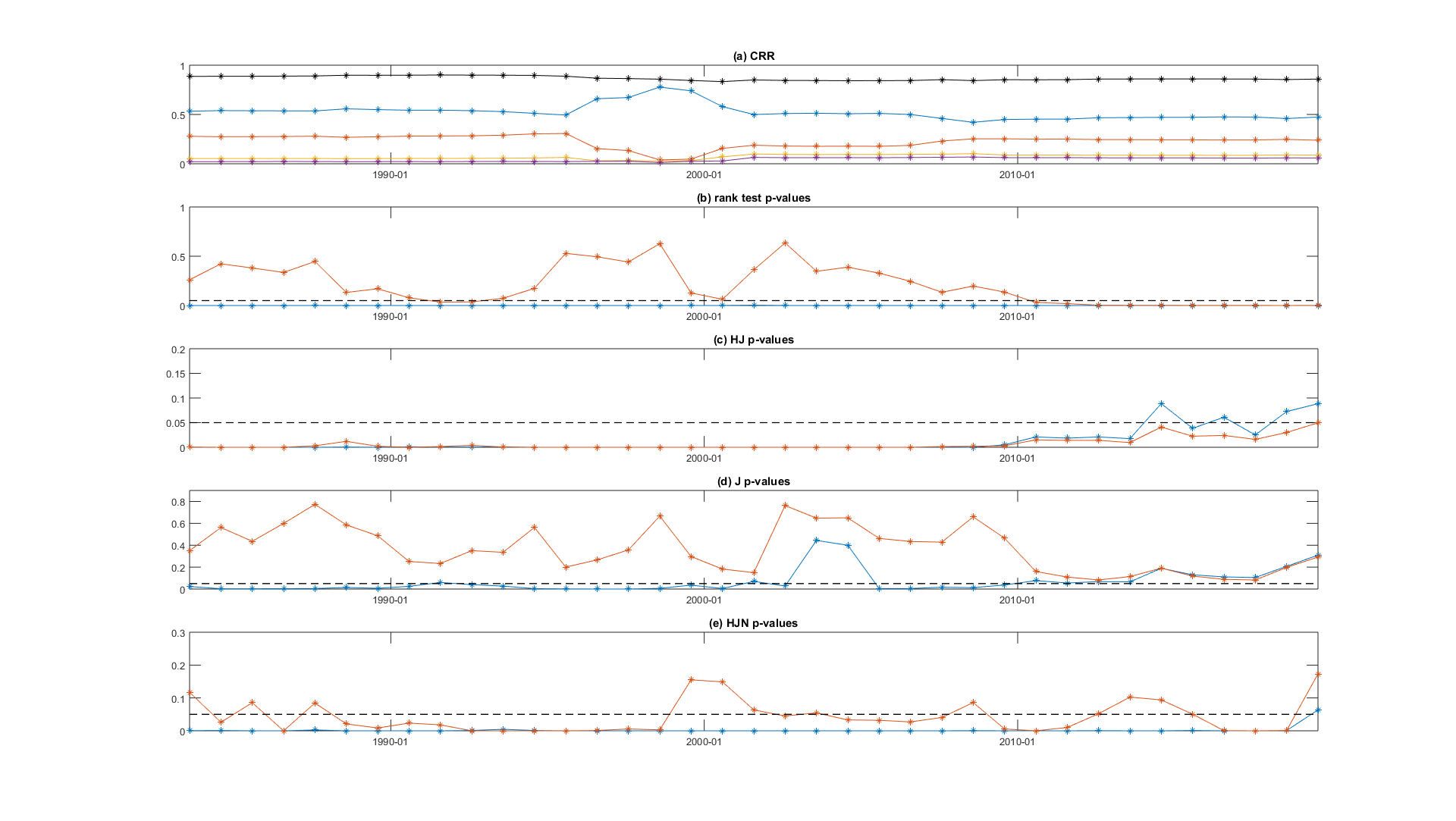
Figure 11: The time series of estimates from 1963-09 to 2019-08 with rolling windows of size T = 240 (20 years) and the number of increments between successive rolling windows being 12 (1 year) (x-axis is labeled with the ending period of each rolling window, for example, the first rolling window uses data from 1963-09 to 1983-08, so x-axis should label the first point with ’1983-08’). (a) The fraction of the total variation of the portfolio returns that is explained by their four largest principal components respectively (CRRs) ($\lambda_{i}/(\sum_{j=1}^{N}\lambda_{j}),i=1,\cdots,4$); the black curve is the fraction of the total variation of the portfolio returns that is explained by the sum of the four largest principal components (sum of the first four CRRs, $\sum_{i=1}^{4}\lambda_{i}/(\sum_{j=1}^{N}\lambda_{j})$); (b) p-values of the rank test (Kleibergen and Paap (2006)) of $q_{G}$ using the estimator $q_{G,T}$ with $G$ constructed by the three FF factors (blue), and the four factors (three FF and momentum factors) (red) respectively; (c) p-values of the HJ specification test of the three-FF-factor model (blue), p-values of the HJ specification test of the four-factor (three FF and momentum factors) model (red); (d) p-values of the $\mathcal{J}$ specification test of the three-FF-factor model (blue), p-values of the HJN specification test of the four-factor (three FF and momentum factors) model (red); (e) p-values of the HJN specification test of the three-FF-factor model (blue), p-values of the HJN specification test of the four-factor (three FF and momentum factors) model (red).

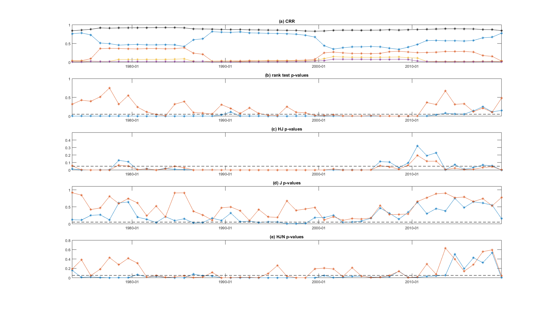
Figure 12: The time series of estimates from 1963-09 to 2019-08 with rolling windows of size T = 240 (20 years) and the number of increments between successive rolling windows being 12 (1 year) (x-axis is labeled with the ending period of each rolling window). (a) The fraction of the total variation of the portfolio returns that is explained by their four largest principal components respectively (CRRs) ($\lambda_{i}/(\sum_{j=1}^{N}\lambda_{j}),i=1,\cdots,4$); the black curve is the fraction of the total variation of the portfolio returns that is explained by the sum of the four largest principal components (sum of the first four CRRs, $\sum_{i=1}^{4}\lambda_{i}/(\sum_{j=1}^{N}\lambda_{j})$); (b) p-values of the rank test (Kleibergen and Paap (2006)) of $q_{G}$ using the estimator $q_{G,T}$ with $G$ constructed by the three FF factors (blue), and the four factors (three FF and momentum factors) (red) respectively; (c) p-values of the HJ specification test of the three-FF-factor model (blue), p-values of the HJ specification test of the four-factor (three FF and momentum factors) model (red); (d) p-values of the $\mathcal{J}$ specification test of the three-FF-factor model (blue), p-values of the HJN specification test of the four-factor (three FF and momentum factors) model (red); (e) p-values of the HJN specification test of the three-FF-factor model (blue), p-values of the HJN specification test of the four-factor (three FF and momentum factors) model (red).

Appendix B Proofs related to sections 2 and 3

Appendices B and C use $\lambda_{j}(A)$ to denote the $j$th largest eigenvalue of a given matrix A, $\lambda_{\min}(A),\lambda_{\max}(A)$ the minimum and the maximum eigenvalues. With $A=(a_{ij})$, multiple matrix norms are denoted as $\left\lVert A\right\rVert=\sqrt{\lambda_{\max}(A^{\prime}A)},\left\lVert A\right\rVert_{1}=\max_{j}\sum_{i}|a_{ij}|,\left\lVert A\right\rVert_{\infty}=\max_{i}\sum_{j}|a_{ij}|,\left\lVert A\right\rVert_{F}=\sqrt{tr(A^{\prime}A)},\left\lVert A\right\rVert_{\max}=\max_{i,j}|a_{ij}|$.

Assumption B.1.

The following asymptotic distributions hold jointly: $\left(\xi_{g,T},\xi_{gg,T},\xi_{vG,T},\xi_{zG,T},\xi_{eG,T},\right)\rightarrow_{d}\left(\xi_{g},\xi_{V},\xi_{vG},\xi_{zG},\xi_{eG}\right)$, where $\xi_{g,T}=\frac{1}{\sqrt{T}}\left(\sum_{t=1}^{T}g_{t}-\mu_{g}\right),$ $\xi_{gg,T}=\frac{1}{\sqrt{T}}\sum_{t=1}^{T}\bar{g}_{t}\bar{g}_{t}^{\prime},$ $\xi_{vG,T}=\frac{1}{\sqrt{T}}\sum_{t=1}^{T}v_{t}G_{t}^{\prime},$$\xi_{zG,T}=\frac{1}{\sqrt{T}}\sum_{t=1}^{T}z_{t}G_{t}^{\prime},$ $\xi_{eG,T}=\frac{1}{\sqrt{T}}\sum_{t=1}^{T}e_{t}G_{t}^{\prime},$ and $\xi_{g},$ $\text{vec}(\xi_{vG}),\text{vec}(\xi_{zG}),$ $\text{vec}(\xi_{eG})$ are zero-mean normal random vectors, $\xi_{V}$ is a Gaussian random matrix.

Assumption B.1 is a central limit theorem for the different components in equation (4) interacted with a constant and the proxy factors. Some of the statements such as $\xi_{g,T}\rightarrow_{d}\xi_{g}$ would hold if proxy factors are stationary with finite fourth moments and satisfy some strong mixing conditions (see e.g. Peligrad et al. (2006)). We specify a relatively strong assumption here instead of dealing with heavy technical details, but our results can be extended to general cases.

Proof of Lemma 2.1.

Assumption 2.1 implies $r_{t}=c+\beta_{g}\bar{g}_{t}+\beta_{g}\left(\bar{g}-\mu_{g}\right)+\beta v_{t}+u_{t}$ then

$$\widehat{B}_{g}= \sum_{i=1}^{T}r_{i}G_{i}^{\prime}\left(\sum_{t=1}^{T}G_{t}G_{t}^{\prime}\right)^{-1}=\sum_{i=1}^{T}\left(c+\beta_{g}\bar{g}_{t}+\beta_{g}\left(\bar{g}-\mu_{g}\right)+\beta v_{t}+u_{t}\right)G_{i}^{\prime}\left(\sum_{t=1}^{T}G_{t}G_{t}^{\prime}\right)^{-1}$$

$$= \left(c,\beta_{g}\right)+\frac{1}{\sqrt{T}}\left(\beta_{g}\xi_{g,T},0\right)+\frac{1}{\sqrt{T}}\left(\beta,\gamma\right)\xi_{vzG,T}\widehat{Q}_{G}^{-1}+\frac{1}{\sqrt{T}}\xi_{eG,T}\widehat{Q}_{G}^{-1}$$

The conclusion is then a direct result from Assumption B.1. ∎

Proof of Theorem 2.2.

Assumption 2.1 and B.1 imply that

$$\widehat{Q}_{r}=Q_{r}+O_{p}(1/\sqrt{T})$$ (16)

$$\iota_{N}={B}_{g}Q_{G}\theta_{G}$$ (17)

Rewrite $T\widehat{\delta}_{g}^{2}$ as

$$\sqrt{T}\left(\iota_{N}-\widehat{B}_{g}Q_{G}\theta_{G}\right)^{\prime}W\sqrt{T}\left(\iota_{N}-\widehat{B}_{g}Q_{G}\theta_{G}\right)$$ (18)

where

$$W=(\widehat{Q}_{r}^{-1}-\widehat{Q}_{r}^{-1}\widehat{B}_{g}Q_{B_{g},T}(Q_{B_{g},T}\widehat{B}_{g}^{\prime}\widehat{Q}_{r}^{-1}\widehat{B}_{g}Q_{B_{g},T})^{-1}Q_{B_{g},T}\widehat{B}_{g}^{\prime}\widehat{Q}_{r}^{-1})$$

$$Q_{B_{g},T}=\text{diag}\left(I_{1+K_{g,1}},\sqrt{T}I_{K_{g,2}}\right)$$

Lemma 2.1 and equation (17) imply that

$$\sqrt{T}\left(\iota_{N}-\widehat{B}_{g}Q_{G}\theta_{G}\right)\rightarrow_{d}\widetilde{\psi}_{B_{g}}$$ (19)

Lemma 2.1 and Assumption 2.3 imply the following equation holds jointly with equation (19)

$$\widehat{B}_{g}Q_{B_{g},T}\rightarrow_{d}\eta_{B_{g}}+(0\vdots\psi_{\beta_{g,2}})$$ (20)

Plug equations (16)(19)(20) in equation (18), then we would derive the conclusion. ∎

Lemma B.1.

Suppose Assumption B.1 and 2.1-2.3 hold, let N,T increase and then the restrictions on $e_{t}$ from Assumption 2.2 (i)(ii)(iii) also hold for $\widetilde{e}_{t}$ with $\widetilde{e}_{t}=Q_{r}^{-\frac{1}{2}}e_{t}$ with $Q_{r}^{-\frac{1}{2}}=A\Lambda^{-\frac{1}{2}}A^{\prime}$ such that $Q_{r}=A\Lambda A^{\prime}$ with $A^{\prime}A=I_{N}$ and we assume $Q_{r}^{-\frac{1}{2}}$ is a row diagonally-dominant matrix.

Proof of Lemma B.1.

$\widetilde{e}_{t},t=1,\cdots,T$ are i.i.d. mean zero random vectors with finite fourth moments by construction. Next we show $\sup_{i}\mathbb{E}\widetilde{e}_{it}^{4}$ is bounded. Assumption 2.1 implies $Q_{r}=c^{\prime}c+\beta V_{f}\beta^{\prime}+\gamma V_{z}\gamma^{\prime}+\Omega_{e}$ and thus we have the following results by eigenvalue inequalities (see e.g. 7.3.P16 of Horn et al. (2013)):

$$\lambda_{\max}\left(Q_{r}\right)=\lambda_{\max}\left(c^{\prime}c+\beta V_{f}\beta^{\prime}+\gamma V_{z}\gamma^{\prime}+\Omega_{e}\right)\leq\lambda_{\max}\left(c^{\prime}c+\beta V_{f}\beta^{\prime}+\gamma V_{z}\gamma^{\prime}\right)+L$$ (21)

$$\lambda_{\min}\left(Q_{r}\right)=\lambda_{\min}\left(c^{\prime}c+\beta V_{f}\beta^{\prime}+\gamma V_{z}\gamma^{\prime}+\Omega_{e}\right)\geq\lambda_{\min}\left(c^{\prime}c+\beta V_{f}\beta^{\prime}+\gamma V_{z}\gamma^{\prime}\right)+l=l$$ (22)

Then by the assumption that $Q_{r}^{-\frac{1}{2}}$ is a row diagonally-dominant matrix we know any row sums of $Q_{r}^{-\frac{1}{2}}$ would be upper bounded by $2l^{-1/2}$ and thus $\sup_{i}\mathbb{E}{e}_{it}^{4}\leq L$ implies that $\sup_{i}\mathbb{E}\widetilde{e}_{it}^{4}$ is bounded. Therefore, Assumption 2.2 (i) holds.

The term $c^{\prime}c+\beta V_{f}\beta^{\prime}+\gamma V_{z}\gamma^{\prime}$ in $Q_{r}$ is a positive semi-definite matrix and we can rewrite that term as $A_{Q_{r}}\Lambda_{Q_{r}}A_{Q_{r}}^{\prime}$ such that $\Lambda_{Q_{r}}$ is a diagonal matrix containing all positive eigenvalues of $c^{\prime}c+\beta V_{f}\beta^{\prime}+\gamma V_{z}\gamma^{\prime}$ and $A_{Q_{r}}$ are the corresponding eigenvectors. Therefore, $Q_{r}=A_{Q_{r}}\Lambda_{Q_{r}}A_{Q_{r}}^{\prime}+\Omega_{e}$ and thus

$$Q_{r}^{-1}=\Omega_{e}^{-1}-\Omega_{e}^{-1}A_{Q_{r}}\left(\Lambda_{Q_{r}}^{-1}+A_{Q_{r}}^{\prime}\Omega_{e}^{-1}A_{Q_{r}}\right)^{-1}A_{Q_{r}}^{\prime}\Omega_{e}^{-1}$$ (23)

which then implies that

$$\text{tr}\left(\mathbb{E}Q_{r}^{-1/2}e_{t}e_{t}^{\prime}Q_{r}^{-1/2}\right)/N=\text{tr}\left(\Omega_{e}Q_{r}^{-1}\right)/N=1-\text{tr}\left(\left(\Lambda_{Q_{r}}^{-1}+A_{Q_{r}}^{\prime}\Omega_{e}^{-1}A_{Q_{r}}\right)^{-1}\right)/N$$

From the fact that the eigenvalues of $\Lambda_{Q_{r}}$ explode by Assumption 2.3 and the eigenvalues of $\Omega_{e}$ are bounded by Assumption 2.2 , Courant-Fischer minimax principle implies $\text{tr}\left(\left(\Lambda_{Q_{r}}^{-1}+A_{Q_{r}}^{\prime}\Omega_{e}^{-1}A_{Q_{r}}\right)^{-1}\right)/N\rightarrow 0$. Furthermore, Assumption 2.2 and 2.3 imply that $\lim\inf_{N,T}\lambda_{\min}\left(Q_{r}^{-1/2}\right)$ and $\lim\sup_{N,T}\lambda_{\min}\left(Q_{r}^{-1/2}\right)$ are bounded, and thus we also have

$$0<l<\lim\inf_{N,T}\lambda_{\min}\left(Q_{r}^{-1/2}\Omega_{e}Q_{r}^{-1/2}\right)<\lim\sup_{N,T}\lambda_{\max}\left(Q_{r}^{-1/2}\Omega_{e}\right)Q_{r}^{-1/2}<L<\infty.$$

Therefore, Assumption 2.2 (ii) holds for $\widetilde{e}_{t}$. As for Assumption 2.2 (iii), inequalities for the trace of matrix product (e.g. Fang et al. (1994)) suggest

$$\lambda_{\min}\left(Q_{r}^{-1}\right)\text{tr}\left(e_{t}e_{t}^{\prime}\right)-\lambda_{\max}\left(Q_{r}^{-1}\right)\text{tr}\left(\mathbb{E}\left(e_{t}e_{t}^{\prime}\right)\right)$$

$$\leq \text{tr}\left(Q_{r}^{-1}\left(e_{t}e_{t}^{\prime}-\mathbb{E}\left(e_{t}e_{t}^{\prime}\right)\right)\right)\leq\lambda_{\max}\left(Q_{r}^{-1}\right)\text{tr}\left(e_{t}e_{t}^{\prime}\right)-\lambda_{\min}\left(Q_{r}^{-1}\right)\text{tr}\left(\mathbb{E}\left(e_{t}e_{t}^{\prime}\right)\right)$$

which implies that $\mathbb{E}\left|\frac{1}{\sqrt{N}}\sum_{i=1}^{N}\left(\widetilde{e}_{it}\widetilde{e}_{is}-\mathbb{E}\widetilde{e}_{it}\widetilde{e}_{is}\right)\right|^{4}<L<\infty$ given all eigenvalues of $Q_{r}^{-1}$ are bounded. ∎

Theorem B.2 illustrates how the weak (proxy) factors can affect the asymptotic properties of the estimator $\widehat{\theta}_{G}$. This theorem resembles Theorem one from Anatolyev and Mikusheva (2018), and indeed we observe that the asymptotic behavior of the estimator $\widehat{\theta}_{G}$ is similar to the one of the two-pass FM risk premia analyzed in Anatolyev and Mikusheva (2018).

Theorem B.2.

Case (1): Suppose Assumption B.1 and 2.1-2.3 hold, N is fixed and T increases to infinity:

$$\sqrt{T}Q_{B_{g},T}^{-1}\left(\widehat{Q}_{G}(\widehat{\theta}_{G}-{\theta}_{G})-\textit{bias}_{e}-\textit{bias}_{m}\right)=O_{p}(1)$$

where

$$\textit{bias}_{e}=-\left(\widehat{B}_{g}^{\prime}\widehat{Q}_{r}^{-1}\widehat{B}_{g}\right)^{-1}\widehat{B}_{g,e}^{\prime}\widehat{Q}_{r}^{-1}\widehat{B}_{g,e}\widehat{Q}_{G}{\theta}_{G}$$

$$\textit{bias}_{m}=-\left(\widehat{B}_{g}^{\prime}\widehat{Q}_{r}^{-1}\widehat{B}_{g}\right)^{-1}\left({B}_{g}+\widehat{B}_{g,m}\right)^{\prime}\widehat{Q}_{r}^{-1}\widehat{B}_{g,m}\widehat{Q}_{G}{\theta}_{G}$$

$$\widehat{B}_{g,e}=\frac{1}{\sqrt{T}}\xi_{eG,T}\widehat{Q}_{G}^{-1};~{}\widehat{B}_{g,m}=\frac{1}{\sqrt{T}}\left(\beta,\gamma\right)\xi_{vzG,T}\widehat{Q}_{G}^{-1};~{}Q_{B_{g},T}=\textit{diag}\left(I_{1+K_{g,1}},\sqrt{T}I_{K_{g,2}}\right)$$

and

$$\sqrt{T}Q_{B_{g},T}^{-1}\textit{bias}_{e}=\left(\begin{matrix}\sqrt{T}\textit{bias}_{e,1}\\ \textit{bias}_{e,2}\end{matrix}\right)\rightarrow_{d}WQ_{B_{g}}\widetilde{e}^{\prime}Q_{r}^{-1}\widetilde{e}Q_{G}\theta_{G}$$

$$\sqrt{T}Q_{B_{g},T}^{-1}\textit{bias}_{m}=\left(\begin{matrix}\sqrt{T}\textit{bias}_{m,1}\\ \textit{bias}_{m,2}\end{matrix}\right)\rightarrow_{d}W\left(\left(\begin{matrix}I_{1+K_{g}}\\ 0\end{matrix}\right)+\widetilde{\xi}Q_{B_{g}}\right)^{\prime}\eta^{\prime}Q_{r}^{-1}\eta\widetilde{\xi}Q_{G}\theta_{G}$$

$$W=-\left(\left(\eta\left(\left(\begin{matrix}I_{1+K_{g}}\\ 0\end{matrix}\right)+\widetilde{\xi}Q_{B_{g}}\right)+\widetilde{e}Q_{B_{g}}\right)^{\prime}Q_{r}^{-1}\left(\eta\left(\left(\begin{matrix}I_{1+K_{g}}\\ 0\end{matrix}\right)+\widetilde{\xi}Q_{B_{g}}\right)+\widetilde{e}Q_{B_{g}}\right)\right)^{-1}$$

Case (2): Suppose Assumption B.1 and 2.1-2.3 hold, let N, T increases to infinity $N/T\rightarrow c$ and $Q_{r}$ is a known row diagonally-dominant matrix such that $\eta^{\prime}Q_{r}^{-1}\eta/N\rightarrow\widetilde{D}$:

$$\sqrt{NT}Q_{B_{g},T}^{-1}\left(\widehat{Q}_{G}(\widehat{\theta}_{G}-{\theta}_{G,T})-\textit{bias}_{e}-\textit{bias}_{m}\right)=O_{p}(1)$$

where

$${\theta}_{G,T}=\theta_{G}+\widehat{Q}_{G}^{-1}\left(\widehat{B}_{g}^{\prime}{Q}_{r}^{-1}\widehat{B}_{g}\right)^{-1}\widehat{B}_{g}^{\prime}{Q}_{r}^{-1}\left(q_{G}\left(\widehat{Q}_{G}^{-1}-{Q}_{G}^{-1}\right)-\frac{1}{\sqrt{T}}\left(\beta_{g}\xi_{g,T},0\right)\right)\widehat{Q}_{G}{\theta}_{G}$$

$$\sqrt{T}Q_{B_{g},T}^{-1}\widehat{Q}_{G}\left({\theta}_{G,T}-\theta_{G}\right)=O_{p}(1)$$

$$\sqrt{T}Q_{B_{g},T}^{-1}\textit{bias}_{e}=\left(\begin{matrix}\sqrt{T}\textit{bias}_{e,1}\\ \textit{bias}_{e,2}\end{matrix}\right)\rightarrow_{d}WQ_{B_{g}}\widetilde{\Sigma}_{{e}}Q_{G}\theta_{G}$$

$$\sqrt{T}Q_{B_{g},T}^{-1}\textit{bias}_{m}=\left(\begin{matrix}\sqrt{T}\textit{bias}_{m,1}\\ \textit{bias}_{m,2}\end{matrix}\right)\rightarrow_{d}W\left(\left(\begin{matrix}I_{1+K_{g}}\\ 0\end{matrix}\right)+\widetilde{\xi}Q_{B_{g}}\right)^{\prime}\widetilde{D}\widetilde{\xi}Q_{G}\theta_{G}$$

$$W=-\left(\left(\left(\begin{matrix}I_{1+K_{g}}\\ 0\end{matrix}\right)+\widetilde{\xi}Q_{B_{g}}\right)^{\prime}\widetilde{D}\left(\left(\begin{matrix}I_{1+K_{g}}\\ 0\end{matrix}\right)+\widetilde{\xi}Q_{B_{g}}\right)+Q_{B_{g}}\widetilde{\Sigma}_{{e}}Q_{B_{g}}\right)^{-1}$$

Proof of Theorem B.2.

Case (1): After simple algebra, we can express the term $\widehat{Q}_{G}\left(\widehat{\theta}_{G}-\theta\right)-\textit{bias}_{e}-\textit{bias}_{m}$ in the following way

$$\widehat{Q}_{G}\left(\widehat{\theta}_{G}-\theta\right)-\textit{bias}_{e}-\textit{bias}_{m}=\left(\widehat{B}_{g}^{\prime}\widehat{Q}_{r}^{-1}\widehat{B}_{g}\right)^{-1}\left\{\widehat{B}_{g}^{\prime}\widehat{Q}_{r}^{-1}\left(q_{G}\left(\widehat{Q}_{G}^{-1}-{Q}_{G}^{-1}\right)-\frac{1}{\sqrt{T}}\left(\beta_{g}\xi_{g,T},0\right)\right)\right.$$

$$\left.-\left(\frac{1}{\sqrt{T}}\left(\beta_{g}\xi_{g,T},0\right)+\widehat{B}_{g,e}\right)^{\prime}\widehat{Q}_{r}^{-1}\widehat{B}_{g,m}-\left(B_{g}+\frac{1}{\sqrt{T}}\left(\beta_{g}\xi_{g,T},0\right)+\widehat{B}_{g,m}\right)^{\prime}\widehat{Q}_{r}^{-1}\widehat{B}_{g,e}\right\}\widehat{Q}_{G}{\theta}_{G}$$ (24)

From the proofs of Lemma 2.1 and Theorem 2.2 we have

$$\widehat{B}_{g}=B_{g}+\frac{1}{\sqrt{T}}\left(\beta_{g}\xi_{g,T},0\right)+\widehat{B}_{g,m}+\widehat{B}_{g,e}$$ (25)

$$\widehat{B}_{g}Q_{B_{g},T}=\left(c+O_{p}(1/\sqrt{T}),\eta_{\beta_{g}}\right)+\left(\frac{1}{\sqrt{T}}\widetilde{e}_{T}+\frac{1}{\sqrt{T}}\eta\widetilde{\xi}_{T}\right)Q_{B_{g},T}$$ (26)

where $\widetilde{\xi}_{T}=\sqrt{T}\widehat{B}_{g,m}=\left(\begin{matrix}0&0\\ \left(d_{g}Q_{\beta_{g}}\right)^{-1}&0\\ 0&I_{K_{z}}\end{matrix}\right)\xi_{vzG,T}\widehat{Q}_{G}^{-1},~{}~{}\widetilde{e}_{T}=\sqrt{T}\widehat{B}_{g,e}=\xi_{eG,T}\widehat{Q}_{G}^{-1},$$\widetilde{\xi}_{T}\rightarrow_{d}\widetilde{\xi},\widetilde{e}_{T}\rightarrow_{d}\widetilde{e},Q_{B_{g},T}/{\sqrt{T}}\rightarrow Q_{B_{g}}=\text{diag}\left(0_{1+K_{g,1}},I_{K_{g,2}}\right)$ and $\widetilde{\xi},\widetilde{e}$ are Gaussian random matrices. Equation (26) implies that

$$\widehat{B}_{g}Q_{B_{g},T}\rightarrow_{d} ~{}~{}\eta\left(\left(\begin{matrix}I_{1+K_{g}}\\ 0\end{matrix}\right)+\widetilde{\xi}Q_{B_{g}}\right)+\widetilde{e}Q_{B_{g}}$$ (27)

With the above intermediate results, we prove our statement for the term $\textit{bias}_{e}$ and the rests follow the same steps. Assumption B.1 implies that the above asymptotic results hold jointly and thus if we plug these into the equation below we would derive the asymptotic distribution of the term $\textit{bias}_{e}$

$$\sqrt{T}Q_{B_{g},T}^{-1}\textit{bias}_{e}=-\left((\widehat{B}_{g}Q_{B_{g},T})^{\prime}\widehat{Q}_{r}^{-1}(\widehat{B}_{g}Q_{B_{g},T})\right)^{-1}(\widehat{B}_{g,e}Q_{B_{g},T})^{\prime}\widehat{Q}_{r}^{-1}(\sqrt{T}\widehat{B}_{g,e})\widehat{Q}_{G}{\theta}_{G}$$ (28)

Case (2): Next we discuss the case where N,T both grows to infinity. We first show the following two results:

$$(2.1)~{}~{}T\widetilde{e}_{T}^{\prime}Q_{r}^{-1}\widetilde{e}_{T}/N\rightarrow_{p}\tilde{\Sigma}_{e}$$ (29)

$$(2.2)~{}~{}\sqrt{T}\widetilde{e}_{T}^{\prime}Q_{r}^{-1}\eta/N\rightarrow_{p}0$$ (30)

To prove statement (2.1), let $\widetilde{e}_{t}=Q_{r}^{-\frac{1}{2}}e_{t}$ and $\rho(s,t)=\frac{1}{\sqrt{N}}\sum_{i=1}^{N}\widetilde{e}_{it}^{\prime}\widetilde{e}_{is}$. By construction, $\mathbb{E}\rho^{2}(s,t)=\frac{1}{N}\text{tr}\left(\Omega_{\widetilde{e}}\Omega_{\widetilde{e}}\right)\leq\lambda_{\max}^{2}(\Omega_{\widetilde{e}})$ with $\Omega_{\widetilde{e}}=\mathbb{E}\widetilde{e}_{t}\widetilde{e}_{t}^{\prime}$ and thus Lemma B.1 implies that $\mathbb{E}\rho^{2}(s,t)$ is bounded. Assumption 2.1 (finite fourth moments of proxy factors), Assumption 2.2 (i) and the bounded $\mathbb{E}\rho^{2}(s,t)$ deliver the following inequality

$$\mathbb{E}\left(\frac{1}{T\sqrt{N}}\sum_{i=1}^{N}\left(\sum_{t=1}^{T}\sum_{s\neq t}^{T}G_{tm}G_{sn}\widetilde{e}_{it}^{\prime}\widetilde{e}_{is}\right)\right)^{2}$$

$$= \mathbb{E}\left(\frac{1}{T}\left(\sum_{t=1}^{T}\sum_{s\neq t}^{T}G_{tm}G_{sn}\rho(s,t)\right)\right)\left(\frac{1}{T}\left(\sum_{t^{\prime}=1}^{T}\sum_{s^{\prime}\neq t}^{T}G_{t^{\prime}m}G_{s^{\prime}n}\rho(s^{\prime},t^{\prime})\right)\right)$$

$$= \mathbb{E}\left(\frac{1}{T^{2}}\left(\sum_{t=1}^{T}\sum_{s\neq t}^{T}\left(G^{2}_{tm}G^{2}_{sn}+G_{tm}G_{sn}G_{sm}G_{tn}\right)\rho^{2}(s,t)\right)\right)<L$$ (31)

which with Chebyshev’s inequality gives

$$\frac{1}{T\sqrt{N}}\sum_{i=1}^{N}\left(\sum_{t=1}^{T}\sum_{s\neq t}^{T}G_{t}G_{s}^{\prime}\widetilde{e}_{it}^{\prime}\widetilde{e}_{is}\right)=O_{P}(1)$$ (32)

Finally we arrive at (2.1):

$$T\widetilde{e}_{T}^{\prime}Q_{r}\widetilde{e}_{T}/N =\widehat{Q}_{g}^{-1}\left(\frac{1}{N{T}}\sum_{t=1}^{T}G_{t}\widetilde{e}_{t}^{\prime}\widetilde{e}_{t}G_{t}^{\prime}\right)\widehat{Q}_{g}^{-1}+O_{p}(1/\sqrt{N})=\tilde{\Sigma}_{e}+O_{p}(1/\sqrt{N})$$ (33)

where the first equality is due to equation (32) and the last equality is guaranteed by Lemma B.1.

Next, we prove the statement (2.2). We first look at the second moments

$$\mathbb{E}\left(\left\|\frac{1}{\sqrt{T}}\sum_{t=1}^{T}G_{t}e_{t}^{\prime}Q_{r}^{-1}\eta/\sqrt{N}\right\|^{2}\right)\leq\mathbb{E}\left(\text{tr}\left(\frac{1}{\sqrt{T}}\sum_{t=1}^{T}G_{t}\widetilde{e}_{t}^{\prime}Q_{r}^{-1/2}\eta/\sqrt{N}\right)\left(\frac{1}{\sqrt{T}}\sum_{t=1}^{T}G_{t}\widetilde{e}_{t}^{\prime}Q_{r}^{-1/2}\eta/\sqrt{N}\right)^{\prime}\right)$$

$$= \frac{1}{{T}}\sum_{t=1}^{T}\text{tr}\left(\mathbb{E}\left(G_{t}\widetilde{e}_{t}^{\prime}Q_{r}^{-1/2}\eta\eta^{\prime}Q_{r}^{-1/2}\widetilde{e}_{t}G_{t}^{\prime}\right)/{N}\right)\leq L\text{tr}\left(\Omega_{\widetilde{e}}Q_{r}^{-1/2}\eta\eta^{\prime}Q_{r}^{-1/2}/{N}\right)\leq L\lambda_{\max}\left(\Omega_{\widetilde{e}}\right)\left\lVert Q_{r}^{-1/2}\right\rVert^{2}_{1}(\left\lVert\eta\right\rVert^{2}_{F}/N)$$

where the first inequality is because factors $g_{t}$ have finite fourth moments. The proof of Lemma B.1 shows that $\lambda_{\max}\left(\Omega_{\widetilde{e}}\right)$ and $\left\lVert Q_{r}^{-1/2}\right\rVert^{2}_{1}$ are bounded, Assumption 2.3 implies that $\left\lVert\eta\right\rVert^{2}_{F}/N$ is bounded. Therefore, we know

$$\mathbb{E}\left(\left\|\frac{1}{\sqrt{T}}\sum_{t=1}^{T}G_{t}e_{t}^{\prime}Q_{r}^{-1}\eta/\sqrt{N}\right\|^{2}\right)\leq L<\infty$$ (34)

and thus (2.2) holds since $\sqrt{T}\widetilde{e}_{T}^{\prime}Q_{r}^{-1}\eta/N=\frac{1}{\sqrt{N}}{Q}_{g}^{-1}\left(\frac{1}{\sqrt{T}}\sum_{t=1}^{T}G_{t}e_{t}^{\prime}Q_{r}^{-1}\eta/\sqrt{N}\right)=O_{p}(1/\sqrt{N})$. In the end, $\eta^{\prime}Q_{r}^{-1}\eta/N\rightarrow\widetilde{D}$ and the result (2.2) imply the following term is of order $O_{p}(1)$ when $N/T\rightarrow c$:

$$\frac{\sqrt{T}}{\sqrt{N}}{Q}_{B_{g},T}\left\{-\left(\frac{1}{\sqrt{T}}\left(\beta_{g}\xi_{g,T},0\right)+\frac{1}{\sqrt{T}}\widetilde{e}_{T}\right)^{\prime}{Q}_{r}^{-1}\frac{1}{\sqrt{T}}\widetilde{\xi}_{T}-\left(B_{g}+\frac{1}{\sqrt{T}}\left(\beta_{g}\xi_{g,T},0\right)+\frac{1}{\sqrt{T}}\widetilde{\xi}_{T}\right)^{\prime}{Q}_{r}^{-1}\frac{1}{\sqrt{T}}\widetilde{e}_{T}\right\}=O_{p}(1)$$

∎

Assumption B.2.

Let $e_{g,t}({\theta}_{G})=\iota_{N}-r_{t}G_{t}^{\prime}{\theta}_{G}$, and the restrictions on $e_{t}$ from Assumption 2.2 (i)(ii)(iii) also hold for $e_{g,t}({\theta}_{G})$.

Proof of Corollary 2.2.2.

Theorem 2.2 suggest for given $N$, $T\widehat{\delta}^{2}_{g}\rightarrow_{d}d_{1,N}$ with $d_{1,N}=\widetilde{\psi}_{B_{g}}^{\prime}M_{Q_{r}^{-\frac{1}{2}}\left(\eta_{B_{g}}+(0\vdots\psi_{\beta_{g,2}})\right)}\widetilde{\psi}_{B_{g}},$ $\widetilde{\psi}_{B_{g}}\sim N(0,S_{B_{g}})$ and $S_{B_{g}}=p\lim S_{B_{g},T},S_{B_{g},T}=\frac{1}{T}\sum_{t=1}^{T}e_{g,t}({\theta}_{G})e_{g,t}({\theta}_{G})^{\prime}$. From the construction of the $\widehat{c}_{1-\alpha}$, we know it is drawn from the distribution of the $d_{2,N}={\psi}_{S}^{\prime}M_{Q_{r}^{-\frac{1}{2}}\left(\eta_{B_{g}}+(0\vdots\psi_{\beta_{g,2}})\right)}{\psi}_{S}$ with $\psi_{S}\sim N(0,S),S=p\lim\widehat{S},\widehat{S}=\frac{1}{T}\sum_{t=1}^{T}{e}_{g,t}(\widehat{\theta}_{G}){e}_{g,t}(\widehat{\theta}_{G})^{\prime},\widehat{e}_{g,t}=\iota_{N}-r_{t}G_{t}^{\prime}\widehat{\theta}_{G}$ and $\psi_{S}$ independent from $\psi_{B_{g}}$. The proof of Theorem B.2 suggest that $\widetilde{\psi}_{B_{g}}^{\prime}P_{Q_{r}^{-\frac{1}{2}}\left(\eta_{B_{g}}+(0\vdots\psi_{\beta_{g,2}})\right)}\widetilde{\psi}_{B_{g}}=O_{p}(1)$ for any given N, and the same for the term ${\psi}_{S}^{\prime}P_{Q_{r}^{-\frac{1}{2}}\left(\eta_{B_{g}}+(0\vdots\psi_{\beta_{g,2}})\right)}{\psi}_{S}$. Now we look at the difference $S_{B_{g},T}-S_{T}$.

$$S_{T}= \frac{1}{T}\sum_{t=1}^{T}\left(\iota_{N}-r_{t}G_{t}^{\prime}\left(\widehat{\theta}_{G}-\theta_{G}+\theta_{G}\right)\right)\left(\iota_{N}-r_{t}G_{t}^{\prime}\left(\widehat{\theta}_{G}-\theta_{G}+\theta_{G}\right)\right)^{\prime}$$

$$= S_{B_{g},T}+\frac{1}{T}\sum_{t=1}^{T}\left(r_{t}G_{t}^{\prime}\left(\widehat{\theta}_{G}-\theta_{G}\right)\right)\left(r_{t}G_{t}^{\prime}\left(\widehat{\theta}_{G}-\theta_{G}\right)\right)^{\prime}$$

$$-\frac{1}{T}\sum_{t=1}^{T}\left(r_{t}G_{t}^{\prime}\left(\widehat{\theta}_{G}-\theta_{G}\right)\right)e_{g,t}^{\prime}-\frac{1}{T}\sum_{t=1}^{T}e_{g,t}\left(r_{t}G_{t}^{\prime}\left(\widehat{\theta}_{G}-\theta_{G}\right)\right)^{\prime}$$ (35)

Assumption B.2 and proofs of Theorem B.2 then suggest the last two terms be negligible in large samples, and thus for fixed $N$ when $T$ is large $S_{T}\approx S_{B_{g},T}+\frac{1}{T}\sum_{t=1}^{T}\left(r_{t}G_{t}^{\prime}\left(\widehat{\theta}_{G}-\theta_{G}\right)\right)\left(r_{t}G_{t}^{\prime}\left(\widehat{\theta}_{G}-\theta_{G}\right)\right)^{\prime}$. This then lead to the conclusion. ∎

Proof of Lemma 3.1.

Assumption B.2 implies that for $\theta_{G}$, $AR(\theta_{G})\rightarrow_{d}\chi^{2}(N)$ which then implies the result. ∎

Proof of Theorem 3.2.

Notice if $\theta_{G}\in CS_{r,\alpha_{1}}$ then $T\widehat{\delta}_{g}^{*}\leq Te_{g,T}(\theta_{G})^{\prime}{Q}_{r}^{-1}e_{g,T}(\theta_{G})$ and $c_{1-\alpha_{2}}(\theta_{G})\leq c_{1-\alpha}^{*}$. Assumption B.2 implies in large samples

$$\lim\inf\limits_{T}\mathbb{P}\left(Te_{g,T}(\theta_{G})^{\prime}{Q}_{r}^{-1}e_{g,T}(\theta_{G})\leq c_{1-\alpha_{2}}(\theta_{G})\right)=1-\alpha_{2}$$

The Lemma 3.1 and $(1-\alpha_{1})(1-\alpha_{2})=1-\alpha$ lead to conclusion. ∎

Proof of Theorem 3.3.

We first provide the proof related with the $\mathcal{J}$ statistic, which essentially results from the proof of Theorem 2 in Gospodinov et al. (2017).

Denote $W=TL^{\prime}\widehat{B}_{g}^{\prime}P_{1}\left(P_{1}^{\prime}{\Sigma}P_{1}\right)^{-1}P_{1}^{\prime}\widehat{B}_{g}L$, where $P_{1}$ is an $N\times(N-1)$ orthogonal matrix whose columns are orthogonal to $\iota_{N}$ such that $P_{1}^{\prime}P_{1}=I_{N-1},P_{1}P-1^{\prime}=M_{\iota_{N}}$; L is an lower triangular matrix such that ${Q}_{\widetilde{G}}=LL^{\prime}$ and ${\Sigma}$ is the covariance matrix. Define $Z=(P_{1}^{\prime}\Sigma P_{1})^{-1/2}P_{1}^{\prime}\widehat{B}_{g}L$ and $M=(P_{1}^{\prime}\Sigma P_{1})^{-1/2}P_{1}^{\prime}{B}_{g}L$, and then

$$\sqrt{T}\text{vec}\left(Z-M\right)\rightarrow_{d}N(0,I_{(N-1)K})$$

From the assumption on $H$, we know there exists $K\times k$ and $K\times K-k$ matrices $C_{1},C_{2}$ where $(C_{1},C_{2})$ is a $K\times K$ orthogonal matrix and $\widetilde{M}_{1}=MC_{1},\widetilde{M}_{2}=MC_{2}$ are of orders $O({1}/{\sqrt{T}}),O(1)$ respectively. Let $\sqrt{T}\widetilde{M}_{1}\rightarrow\widetilde{\mu}$, then in case (1) $\widetilde{\mu}=0$ and in case (2) $\widetilde{\mu}$ is bounded. Let $\widetilde{Z}=(\widetilde{Z}_{1},\widetilde{Z}_{2})=({Z}C_{1},{Z}C_{2})$ we would have

$$\sqrt{T}\left(\begin{matrix}\text{vec}\left(\widetilde{Z}_{1}\right)\\ \text{vec}\left(\widetilde{Z}_{2}-\widetilde{M}_{2}\right)\end{matrix}\right)\rightarrow_{d}N\left(\left(\begin{matrix}\text{vec}\left(\widetilde{\mu}\right)\\ 0\end{matrix}\right),~{}~{}I_{(N-1)K}\right)$$

The proof of theorem 2 in Gospodinov et al. (2017) shows that: (i) the asymptotic distribution of the $\mathcal{J}$ statistic is the same as the one of the largest eigenvalue, $w_{k}$, of $\widetilde{W}^{-1}$ with

$$\widetilde{W}=T\widetilde{Z}_{1}^{\prime}M_{\widetilde{Z}_{2}}\widetilde{Z}_{1},$$ (36)

and thus (ii) in case (1) where $H$ is of reduced rank and $\widetilde{\mu}=0$, $\widetilde{W}\rightarrow_{d}\mathcal{W}_{k}\left(N-K-1+k,I_{r}\right)$ and

$$\mathbb{P}\left(w_{k}\leq a\right)\leq\mathbb{P}\left(x_{k}\leq a\right),~{}~{}x_{k}\sim\chi^{2}_{N-k},$$

In case (2), where $\widetilde{\mu}\neq 0$, $\widetilde{W}$ follows a non-central Wishart distribution $W_{k}(N-K-1+k,I_{r},\mu)$ with $\mu=\widetilde{\mu}^{\prime}M_{\widetilde{M}_{2}}\widetilde{\mu},\left\lVert\mu\right\rVert\leq L<\infty$ asymptotically, which then implies the inconsistency of the $\mathcal{J}$ test. The consistency of the HJS test is obvious since $\left\lVert\iota_{N}-q_{\widetilde{G}}\theta_{\widetilde{G}}\right\rVert>a>0,\forall\theta_{\widetilde{G}}\in\Theta$ implies that $\left\lVert\iota_{N}-q_{\widetilde{G},T}\theta_{\widetilde{G}}\right\rVert=O_{p}(\sqrt{T}),\forall\theta_{\widetilde{G}}\in\Theta$.

∎

Example B.1.

We use an specific example, where we suppose Assumptions 2.1, - 2.3 hold with $Q_{\widetilde{G}}=\mathbb{E}({G}_{t}{G}_{t}^{\prime})$, $K\geq K_{g,2}\geq 1$, to show that over the supreme, $T\sup_{\theta\in CS_{r,\alpha_{1}}}\delta_{g,T}(\theta)$, is not properly bounded by $c_{1-\alpha}^{*}$ in the sense that there would be $\alpha>0$ such that

$$\lim\inf_{T}\mathbb{P}\left(\left(T\sup_{\theta\in CS_{r,\alpha_{1}}}\delta_{g,T}(\theta)\right)\geq c_{1-\alpha}^{*}\right)>\alpha.$$

We prove this by discussing elements in the confidence set. We group $\theta$s in $CS_{r,\alpha_{1}}$ into two classes: (1) $\theta$s with entries corresponding to strong proxy factors deviating from their true values; (2) $\theta$s with entries corresponding to weak proxy factors deviating from their true values. Notice for any $\theta$s belong to class (1), $T\delta_{g,T}(\theta)$ is of order $O_{p}(T)$, while for $\theta$s belong to class (2) we have $T\delta_{g,T}(\theta)=T\delta_{g,T}(\theta_{G})+O_{p}(1),$ and ${S}_{T}(\theta)={S}_{T}(\theta_{G})+O_{p}(1/\sqrt{T})$.

Now we only need to show that the confidence set in the presence of weak proxy factors contains some $\theta$s in class-(2) with positive probability $\widetilde{\alpha}_{1}\geq l>0$ in large samples, which then leads to the conclusion. The proof of Theorem 1 in Gospodinov et al. (2017) implies that

$$\mathcal{J}(\theta)=CD(\theta)+T\frac{\left(\iota_{N}^{\prime}S_{T}(\theta)^{-1}\left(\iota_{N}-q_{G,T}\theta\right)\right)^{2}}{\iota_{N}^{\prime}S_{T}(\theta)^{-1}\iota_{N}}+O_{p}(\frac{1}{\sqrt{T}})$$

where $CD(\theta)=T\theta^{\prime}q_{G,T}^{\prime}P_{1}\left(\left(\theta^{\prime}\otimes P_{1}^{\prime}\right)\widehat{V}\left(\sqrt{T}\text{vec}(q_{G,T})\right)\left(\theta\otimes P_{1}\right)\right)P_{1}^{\prime}q_{G,T}\theta$. Notice $\inf_{\theta}CD(\theta)$ is a rank test (Kleibergen and Paap (2006)), and in the presence of weak factors $CD\left(\theta_{G}+(0_{K\times 1},1)\right)$ converges to a non-central chi-square distribution which would then implies our claim.

Appendix C Consistency of the $\theta$ estimator

Proofs related to section 4 relies heavily on the properties of our four-pass estimator, and thus we first discuss our four-pass estimator before we provide proofs. This section contains the following results: (1) the number of the strong factors can be estimated consistently; (2) the common component can be estimated consistently when $\sqrt{N}/T\rightarrow 0$; (3) finally, we show that our proposed estimator consistently estimates $\theta$ even in the presence of weak identification issues and we also derive its asymptotic distribution.

Assumption C.1.

$\left\lVert(\beta;\gamma)_{i}\right\rVert=\left\lVert c_{\beta\gamma,i}\right\rVert\leq L$. $Q_{(\beta;\gamma)}=\lim\limits_{N\rightarrow\infty}(\beta;\gamma)^{\prime}(\beta;\gamma)/N$ with $Q_{(\beta;\gamma)}$ a $K_{vz}\times K_{vz}$ positive definite matrix with $0<l\leq\lambda_{K_{g}}\left(Q_{(\beta;\gamma)}\right)\leq\lambda_{1}\left(Q_{(\beta;\gamma)}\right)<L<\infty$. (Assumption 2.3 implies this assumption via the Ostrowski theorem and some extra mild assumptions on $Q_{r}$.) such that

$$\left\lVert N^{-1}c_{\beta\gamma}^{\prime}c_{\beta\gamma}-Q_{\beta\gamma}\right\rVert=o_{p}(1)$$

Assumption C.2.

Let $\gamma_{N}(t,t^{\prime})=\mathbb{E}\left(N^{-1}\sum_{i=1}^{N}e_{it}e_{it^{\prime}}\right)$, there exists a positive constant $L$ such that

$$(1)~{}T^{-1}\sum_{t=1}^{T}\sum_{t^{\prime}=1}^{T}\lvert\gamma_{N}(t,t^{\prime})\rvert\leq L;\max_{t}|\gamma_{N}(t,t^{\prime})|\leq L$$

$$(2)~{}T^{-2}\sum_{t=1}^{T}\sum_{t^{\prime}=1}^{T}\mathbb{E}\left(\sum_{i=1}^{N}e_{it}e_{it^{\prime}}-\mathbb{E}\left(\sum_{i=1}^{N}e_{it}e_{it^{\prime}}\right)\right)^{2}=T^{-2}\sum_{t=1}^{T}\sum_{t^{\prime}=1}^{T}\left(\mathbb{E}\left(\sum_{i=1}^{N}e_{it}e_{it^{\prime}}\right)^{2}-N^{2}\gamma_{N}(t,t^{\prime})^{2}\right)\leq LN$$

Assumption C.2 is implied by Assumption 2.2.

Assumption C.3.

$\mathbb{E}\left|\frac{1}{\sqrt{N}}\sum_{i=1}^{N}\left(e_{it}e_{is}-\mathbb{E}e_{it}e_{is}\right)\right|^{4}<L<\infty$

Assumption C.4.

This is implied by Assumptions 2.1 and 2.2 (Weak dependence between proxy factors and Idiosyncratic Errors from Bai and Ng (2002))

$$(i)~{}~{}\mathbb{E}\left(\frac{1}{N}\sum_{i=1}^{N}\left\lVert\frac{1}{\sqrt{T}}\sum_{t=1}^{T}g_{t}e_{it}\right\rVert^{2}\right)\leq L$$

$$(ii)~{}~{}\mathbb{E}\left(\frac{1}{K_{vz}}\sum_{i=1}^{K_{vz}}\left\lVert\frac{1}{\sqrt{T}}\sum_{t=1}^{T}g_{t}u_{vz,it}\right\rVert^{2}\right)\leq L$$

$$(iii)~{}~{}\mathbb{E}\left(\frac{1}{N}\sum_{i=1}^{N}\left\lVert\frac{1}{\sqrt{T}}\sum_{t=1}^{T}u_{vz,t}e_{it}\right\rVert^{2}\right)\leq L$$

Assumption C.5.

For all N and T,

$$\mathbb{E}\sum_{t=1}^{T}\left(\sum_{i=1}^{N}c_{\beta\gamma,{ij}}e_{it}\right)^{2}\leq LNT$$

$$\mathbb{E}\left(\sum_{t=1}^{T}\sum_{i=1}^{N}c_{\beta\gamma,{ij}}e_{it}\right)^{2}\leq LNT$$ (37)

Assumption C.6.

$$\left\lVert T^{-1}u_{vz}^{\prime}u_{vz}-\Sigma_{vz}\right\rVert_{\max}=O_{p}(T^{-\frac{1}{2}})$$

with $\Sigma_{vz}$ a positive definite matrix.

Assumption C.7.

$$\sup_{t}\mathbb{E}\left\lVert u_{vz,t}\right\rVert^{4}\leq L$$

This is identical to one imposed on factors (Assumption A) in Bai and Ng (2002) and Anatolyev and Mikusheva (2018) impose a slightly stronger assumption.

Assumption C.8.

$$(1) \sum_{t}^{T}\left|\gamma_{N}(s,t)\right|\leq L$$

$$(2) \sum_{i=1}^{N}\left|\tau(i,j)\right|\leq L$$

with $\mathbb{E}e_{it}e_{jt}=\tau_{t}(i,j),\left|\tau_{t}(i,j)\right|\leq\left|\tau(i,j)\right|$.

Assumption C.9.

(i)

$$\frac{1}{NT}\mathbb{E}\left\lVert\sum_{s=1}^{T}\sum_{n=1}^{N}{u}_{vz,s}\left(e_{is}e_{it}-\mathbb{E}(e_{is}e_{it})\right)\right\rVert^{2}\leq L$$

(ii) for each t, as $N\rightarrow\infty$

$$\frac{1}{\sqrt{N}}\sum_{i=1}^{N}c_{\beta\gamma,i}e_{ti}\rightarrow_{d}N(0,\Pi_{t})$$

with $\Pi_{t}=\lim\limits_{N\rightarrow\infty}\frac{1}{N}\sum_{i=1}^{N}\sum_{j=1}^{N}c_{\beta\gamma,i}c_{\beta\gamma,j}^{\prime}\mathbb{E}e_{ti}e_{tj}$. And for all $j=1,\cdots,N$

$$\frac{1}{\sqrt{NT}}\sum_{i=1}^{N}\sum_{t=1}^{T}c_{\beta\gamma,i}\left(e_{ti}e_{tj}-\mathbb{E}e_{ti}e_{tj}\right)=O_{p}(1)$$

(iii)

$$\mathbb{E}\left\lVert\frac{1}{\sqrt{NT}}\sum_{t=1}^{T}\sum_{i=1}^{N}u_{vz,t}c_{\beta\gamma,i}^{\prime}e_{it}\right\rVert^{2}_{F}\leq M$$

Assumption C.9 is identical to Assumption F in Bai (2003).

Step (1): the number of the strong factors can be estimated consistently

In this step we prove that we can estimate the number of the strong factors in the $u_{g,t}$ consistently. Here we only provide one way to estimate the number, the estimation approach is not unique. Bai and Ng (2002) propose multiple consistent estimators for the number of strong factors with different penalty functions. Here we use the one employed in Giglio and Xiu (2017). Under Assumption 2.1, we know

$$r_{t}=\widetilde{c}+\beta d_{g}\bar{g}_{t}+u_{g,t}$$ (38)

with $u_{g,t}=\beta v_{t}+\gamma z_{t}+e_{t},\widetilde{c}=c+\beta d_{g}(\bar{g}-\mu_{g})$. $v_{t}$ is assumed to be of a $K_{g}\times 1$ vector, but the dimension of $z_{t}$ is unknown. We estimate the number $K_{vz}$ of the omitted strong factors by

$$\widehat{K}_{vz}=\arg\min_{K_{g}\leq j\leq K_{vz,\max}}\left(N^{-1}T^{-1}\lambda_{j}\left(\widehat{u}_{g}\widehat{u}_{g}^{\prime}\right)+j\phi(N,T)\right)-1$$ (39)

where $\widehat{u}_{g}$ is $T\times N$ matrix stacked with the residuals $\widehat{u}_{g,t}$, $K_{vz,\max}$ is an arbitrary upper bound for $K_{vz}$ and $\phi(N,T)$ is a penalty function with the properties $\phi(N,T)\rightarrow 0,\phi(N,T)/(N^{-\frac{1}{2}}+T^{-\frac{1}{2}})\rightarrow\infty$. Now we show this estimator is consistent.

Theorem C.1.

Suppose Assumptions 2.1, C.1 - C.6 hold, let N,T increase then

$$\widehat{K}_{vz}\rightarrow_{p}K_{vz}$$

Proof of Theorem C.1.

We basically follow the steps in Giglio and Xiu (2017) with small changes in the middle.

(1) We first prove the claim such that for $1\leq j\leq K_{vz}$

$$\lvert N^{-1}T^{-1}\lambda_{j}\left(\widehat{u}_{g}\widehat{u}_{g}^{\prime}\right)-\lambda_{j}\left((Q_{(\beta;\gamma)})^{\frac{1}{2}}\Sigma_{(v;z)}(Q_{(\beta;\gamma)})^{\frac{1}{2}}\right)\rvert=o_{p}(1)$$ (40)

with $Q_{(\beta;\gamma)}=\lim\limits_{N\rightarrow\infty}(\beta;\gamma)^{\prime}(\beta;\gamma)/N$.

For convenience, in this proof, denote ${c}_{\beta\gamma}=(\beta;\gamma),u_{vz}=(v;z)$.

(1.1) Notice

$$\widehat{u}_{g}\widehat{u}_{g}^{\prime}-M_{\bar{G}}u_{vz}c_{\beta\gamma}^{\prime}c_{\beta\gamma}u_{vz}^{\prime}M_{\bar{G}}=M_{\bar{G}}u_{vz}c_{\beta\gamma}^{\prime}e^{\prime}M_{\bar{G}}+M_{\bar{G}}ec_{\beta\gamma}u_{vz}^{\prime}M_{\bar{G}}+M_{\bar{G}}ee^{\prime}M_{\bar{G}}$$

with $\widehat{u}_{g}=M_{\bar{G}}r$. We show in the following steps that the three terms on the right is negligible when divided by $NT$.

For the term $M_{\bar{G}}ee^{\prime}M_{\bar{G}}$, we have

$$\left\lVert M_{\bar{G}}ee^{\prime}M_{\bar{G}}-n\Gamma_{u}\right\rVert\leq\left\lVert ee^{\prime}-n\Gamma_{u}\right\rVert_{F}+2\left\lVert P_{\bar{G}}ee^{\prime}\right\rVert_{F}+\left\lVert P_{\bar{G}}ee^{\prime}P_{\bar{G}}\right\rVert_{F}$$ (41)

Assumption C.2.(1) implies that

$$\mathbb{E}\left\lVert e\right\rVert_{F}^{2}=\mathbb{E}\sum_{i=1}^{N}\sum_{t=1}^{T}e_{it}^{2}\leq LNT$$ (42)

$$\mathbb{E}\left\lVert\bar{e}\right\rVert_{F}^{2}=T^{-2}\mathbb{E}\sum_{i=1}^{N}\sum_{t=1}^{T}\sum_{t^{\prime}=1}^{T}e_{it}e_{it^{\prime}}=NT^{-2}\sum_{t=1}^{T}\sum_{t^{\prime}=1}^{T}\lvert\gamma_{N}(t,t^{\prime})\rvert\leq LNT^{-1}$$ (43)

Assumption C.2.(2) implies that

$$\mathbb{E}\left\lVert ee^{\prime}-n\Gamma_{u}\right\rVert_{F}^{2}=\sum_{t=1}^{T}\sum_{t^{\prime}=1}^{T}\mathbb{E}\left(\sum_{i=1}^{N}e_{it}e_{it^{\prime}}-\mathbb{E}\left(\sum_{i=1}^{N}e_{it}e_{it^{\prime}}\right)\right)^{2}\leq LNT^{2}$$ (44)

Assumption C.4 implies that

$$\mathbb{E}\left\lVert{{G}}^{\prime}e\right\rVert_{F}^{2}=NT\mathbb{E}\left(\frac{1}{N}\sum_{i=1}^{N}\left\lVert\frac{1}{\sqrt{T}}\sum_{t=1}^{T}G_{t}e_{it}\right\rVert^{2}_{F}\right)\leq LNT$$ (45)

$$\left\lVert{{G}}^{\prime}e\right\rVert_{F}=O_{p}(N^{\frac{1}{2}}T^{\frac{1}{2}});\left\lVert\left(0,\iota_{T}\bar{g}^{\prime}\right)^{\prime}e\right\rVert_{F}=O_{p}(N^{\frac{1}{2}}T^{\frac{1}{2}})$$ (46)

$$\left\lVert{\bar{G}}^{\prime}e\right\rVert_{F}\leq\left\lVert{{G}}^{\prime}e\right\rVert_{F}+\left\lVert\left(0,\iota_{T}\bar{g}^{\prime}\right)^{\prime}e\right\rVert_{F}=O_{p}(N^{\frac{1}{2}}T^{\frac{1}{2}})$$ (47)

$$\left\lVert P_{\bar{G}}e\right\rVert_{F}\leq T^{-1}\left\lVert{\bar{G}}\right\rVert_{F}\left\lVert\left({\bar{G}}^{\prime}{\bar{G}}/T\right)^{-1}\right\rVert_{F}\left\lVert{\bar{G}}^{\prime}e\right\rVert_{F}=O_{p}(N^{\frac{1}{2}})$$ (48)

Then the following holds:

$$\left\lVert M_{\bar{G}}ee^{\prime}M_{\bar{G}}-n\Gamma_{u}\right\rVert\leq \left\lVert ee^{\prime}-n\Gamma_{u}\right\rVert_{F}+2\left\lVert P_{\bar{G}}ee^{\prime}\right\rVert_{F}+\left\lVert P_{\bar{G}}ee^{\prime}P_{\bar{G}}\right\rVert_{F}$$

$$= O_{p}(N^{\frac{1}{2}}T)+O_{p}(NT^{\frac{1}{2}})+O_{p}(N)$$ (49)

From assumption C.4 (1) we would have

$$\mathbb{E}\left\lVert\Gamma_{u}\right\rVert_{F}^{2}=\mathbb{E}\sum_{t=1}^{T}\sum_{t^{\prime}=1}^{T}\lvert\gamma_{N}(t,t^{\prime})\rvert\leq LT$$ (50)

$$\left\lVert M_{\bar{G}}ee^{\prime}M_{\bar{G}}\right\rVert_{F}\leq\left\lVert M_{\bar{G}}ee^{\prime}M_{\bar{G}}-n\Gamma_{u}\right\rVert_{F}+\left\lVert n\Gamma_{u}\right\rVert_{F}=O_{p}(N^{\frac{1}{2}}T)+O_{p}(NT^{\frac{1}{2}})$$

For the term $M_{\bar{G}}u_{vz}c_{\beta\gamma}^{\prime}e^{\prime}M_{\bar{G}}$, we have

$$\left\lVert M_{\bar{G}}u_{vz}c_{\beta\gamma}^{\prime}e^{\prime}M_{\bar{G}}\right\rVert_{F}\leq \left\lVert u_{vz}c_{\beta\gamma}^{\prime}e^{\prime}\right\rVert_{F}+\left\lVert P_{\bar{G}}u_{vz}c_{\beta\gamma}^{\prime}e^{\prime}\right\rVert_{F}+\left\lVert u_{vz}c_{\beta\gamma}^{\prime}e^{\prime}P_{\bar{G}}\right\rVert_{F}+\left\lVert P_{\bar{G}}u_{vz}c_{\beta\gamma}^{\prime}e^{\prime}P_{\bar{G}}\right\rVert_{F}$$

$$\leq \left(2(K_{vz}+1)\right)^{2}\left\lVert u_{vz}c_{\beta\gamma}^{\prime}e^{\prime}\right\rVert_{F}$$ (51)

Assumption C.5 implies that

$$\mathbb{E}\left\lVert ec_{\beta\gamma}\right\rVert_{F}^{2}=\mathbb{E}\sum_{j=1}^{K_{vz}}\sum_{t=1}^{T}\left(\sum_{i=1}^{N}c_{\beta\gamma,{ij}}e_{it}\right)^{2}\leq LNT$$ (52)

and

$$\left\lVert u_{vz}\right\rVert\leq KT\left\lVert T^{-1}u_{vz}^{\prime}u_{vz}\right\rVert_{\max}=O_{p}(T^{\frac{1}{2}})$$ (53)

$$\left\lVert u_{vz}c_{\beta\gamma}^{\prime}e^{\prime}\right\rVert\leq\left\lVert u_{vz}\right\rVert\left\lVert c_{\beta\gamma}^{\prime}e^{\prime}\right\rVert_{F}=O_{p}(N^{\frac{1}{2}}T)$$ (54)

$$\left\lVert M_{\bar{G}}u_{vz}c_{\beta\gamma}^{\prime}e^{\prime}M_{\bar{G}}\right\rVert\leq O_{p}(N^{\frac{1}{2}}T)$$ (55)

Therefore,

$$N^{-1}T^{-1}\lvert\lambda_{j}(\widehat{u}_{g}\widehat{u}_{g}^{\prime})-\lambda_{j}(M_{\bar{G}}u_{vz}c_{\beta\gamma}^{\prime}c_{\beta\gamma}u_{vz}^{\prime}M_{\bar{G}})\rvert=o_{p}(1)$$ (56)

(1.2) To finish the proof of part (1) we only need to show the following two results:

$$(1.2.1)~{}~{}\lvert N^{-1}T^{-1}\lambda_{j}(M_{\bar{G}}u_{vz}c_{\beta\gamma}^{\prime}c_{\beta\gamma}u_{vz}^{\prime}M_{\bar{G}})-T^{-1}\lambda_{j}(M_{\bar{G}}u_{vz}Q_{\beta\gamma}u_{vz}^{\prime}M_{\bar{G}})\rvert=o_{p}(1)$$ (57)

$$(1.2.2)~{}~{}\lvert T^{-1}\lambda_{j}(M_{\bar{G}}u_{vz}Q_{\beta\gamma}u_{vz}^{\prime}M_{\bar{G}})-\lambda_{j}\left((Q_{(\beta;\gamma)})^{\frac{1}{2}}\Sigma_{(v;z)}(Q_{(\beta;\gamma)})^{\frac{1}{2}}\right)\rvert=o_{p}(1)$$ (58)

Equation (57) is a direct result of Assumption C.1 and Weyl’s inequality such that

$$\lvert N^{-1}T^{-1}\lambda_{j}(M_{\bar{G}}u_{vz}c_{\beta\gamma}^{\prime}c_{\beta\gamma}u_{vz}^{\prime}M_{\bar{G}})-T^{-1}\lambda_{j}(M_{\bar{G}}u_{vz}Q_{\beta\gamma}u_{vz}^{\prime}M_{\bar{G}})\rvert$$

$$\leq T^{-1}\left\lVert N^{-1}c_{\beta\gamma}^{\prime}c_{\beta\gamma}-Q_{\beta\gamma}\right\rVert\left\lVert M_{\bar{G}}u_{vz}\right\rVert^{2}=o_{p}(1)$$ (59)

Equation (57) is a direct result of Assumption C.6 and Weyl’s inequality such that

$$\lvert T^{-1}\lambda_{j}(M_{\bar{G}}u_{vz}Q_{\beta\gamma}u_{vz}^{\prime}M_{\bar{G}})-\lambda_{j}\left((Q_{(\beta;\gamma)})^{\frac{1}{2}}\Sigma_{vz}(Q_{(\beta;\gamma)})^{\frac{1}{2}}\right)\rvert$$

$$\leq L\left\lVert T^{-1}u_{vz}^{\prime}u_{vz}-\Sigma_{vz}\right\rVert=O_{p}(T^{-\frac{1}{2}})$$ (60)

Therefore, for $1\leq j\leq K_{vz}$, we have

$$\lvert N^{-1}T^{-1}\lambda_{j}\left(\widehat{u}_{g}\widehat{u}_{g}^{\prime}\right)-\lambda_{j}\left((Q_{(\beta;\gamma)})^{\frac{1}{2}}\Sigma_{(v;z)}(Q_{(\beta;\gamma)})^{\frac{1}{2}}\right)\rvert=o_{p}(1)$$ (61)

(2) In part (2) we finish the proof of the consistency $\widehat{K}_{vz}$ by showing the following statement

$$\lim\inf\limits_{T,N\rightarrow\infty}\mathbb{P}\left(\widehat{F}(K_{vz}+1)\leq\widehat{F}(j),j=1,\cdots,N\right)=1$$ (62)

with $\widehat{F}({j})=N^{-1}T^{-1}\lambda_{j}\left(\widehat{u}_{g}\widehat{u}_{g}^{\prime}\right)+j\phi(N,T)$. Notice a direct result from step (1) is that for $1\leq j\leq K_{vz},$ we can find $l>0$ such that $\widehat{F}({j})>l+o_{p}(1)$, while for $K_{vz}+1\leq j,$ $\widehat{F}({j})=o_{p}(1)$. Then we only need to show that for $j>K_{vz}+1$, $\widehat{F}({j})>\widehat{F}(K_{vz}+1)$ with probability approaching to one. Notice for $j\geq K_{vz}+1$,

$$\lambda_{j}\left(\widehat{u}_{g}\widehat{u}_{g}^{\prime}\right)\leq\left\lVert ee^{\prime}\right\rVert=O_{p}(TN^{-\frac{1}{2}}+T^{-\frac{1}{2}}N)$$ (63)

and this implies $\widehat{F}({j})>\widehat{F}(K_{vz}+1)$ with probability approaching to one as $(N^{\frac{1}{2}}T^{\frac{1}{2}})(j-K_{vz}-1)\phi(N,T)>(N^{-\frac{1}{2}}T^{-\frac{1}{2}})\left(\lambda_{K_{vz}+1}\left(\widehat{u}_{g}\widehat{u}_{g}^{\prime}\right)-\lambda_{j}\left(\widehat{u}_{g}\widehat{u}_{g}^{\prime}\right)\right)$ with probability approaching to one.

∎

Step (2): the common component can be estimated consistently when $\sqrt{N}/T\rightarrow 0$

Denote $m_{NT}=\min\{N,T\}$.

Lemma C.2.

Suppose Assumptions 2.1 - 2.2, C.1 - C.6 hold, let N,T increase then

$$m_{NT}\frac{1}{T}\sum_{t=1}^{T}\left\lVert\widetilde{u}_{vz,t}-H^{\prime}u_{vz,t}\right\rVert_{F}^{2}=O_{p}(1)$$

with $H=\left(c_{\beta\gamma}^{\prime}c_{\beta\gamma}/N\right)\left(u_{vz}^{\prime}\widetilde{u}_{vz}/T\right)V_{NT}$ and $V_{NT}$ being the $K_{vz}\times K_{vz}$ diagonal matrix of $\lambda_{i}\left(\widehat{u}_{g}\widehat{u}_{g}^{\prime}/NT\right),i=1,\cdots,K_{vz}$.

Proof of Lemma C.2.

This proof resembles the proof of Theorem 1 in Bai and Ng (2002). From the normalization $\widetilde{u}_{vz}^{\prime}\widetilde{u}_{vz}/T=I_{K_{vz}}$ we know

$$\left\lVert\widetilde{u}_{vz}\right\rVert_{F}^{2}=\sum_{t=1}^{T}\left\lVert\widetilde{u}_{vz,t}\right\rVert_{F}^{2}=O_{p}(T)$$ (64)

From the proof in section and the above equation we know

$$\left\lVert H\right\rVert_{F}\leq\left\lVert c_{\beta\gamma}^{\prime}c_{\beta\gamma}/N\right\rVert_{F}\left\lVert u_{vz}^{\prime}{u}_{vz}/T\right\rVert_{F}^{1/2}\left\lVert\widetilde{u}_{vz}^{\prime}\widetilde{u}_{vz}/T\right\rVert_{F}^{1/2}=O_{p}(1)$$ (65)

From equations (80) and (40), we know

$$\left\lVert\widetilde{u}_{vz,t}-H^{\prime}u_{vz,t}\right\rVert_{F}^{2}\leq L\sum_{i=1}^{6}a_{i,t}^{2}$$ (66)

with

$$a_{1,t}^{2}= T^{-2}\left\lVert\sum_{s=1}^{T}\widetilde{u}_{vz,s}\gamma_{N}(s,t)\right\rVert_{F}^{2}$$

$$a_{2,t}^{2}= T^{-2}\left\lVert\sum_{s=1}^{T}\widetilde{u}_{vz,s}\zeta_{ee,st}\right\rVert_{F}^{2}$$

$$a_{3,t}^{2}= T^{-2}\left\lVert\sum_{s=1}^{T}\widetilde{u}_{vz,s}\zeta_{ue,st}\right\rVert_{F}^{2}$$

$$a_{4,t}^{2}= T^{-2}\left\lVert\sum_{s=1}^{T}\widetilde{u}_{vz,s}\zeta_{eu,st}\right\rVert_{F}^{2}$$

$$a_{5,t}^{2}= \left\lVert\frac{1}{NT}\widetilde{u}_{vz}^{\prime}P_{\bar{G}}u_{g}u_{g,t}^{\prime}\right\rVert_{F}^{2}$$

$$a_{6,t}^{2}= \left\lVert\frac{1}{NT}\widetilde{u}_{vz}^{\prime}M_{\bar{G}}u_{g}\left(\widehat{u}_{g,t}-u_{g,t}\right)\right\rVert_{F}^{2}$$ (67)

From equation (64) and Assumption C.2 (i),

$$\sum_{t=1}^{T}a_{1,t}^{2}\leq\left(T^{-1}\sum_{s=1}^{T}\left\lVert\widetilde{u}_{vz,s}\right\rVert_{F}^{2}\right)\left(T^{-1}\sum_{t=1}^{T}\sum_{s=1}^{T}\gamma_{N}(s,t)^{2}\right)=O_{p}(1)$$ (68)

From equation (64) and Assumption 2.2,

$$\sum_{t=1}^{T}a_{2,t}^{2}\leq\left(T^{-1}\sum_{s=1}^{T}\left\lVert\widetilde{u}_{vz,s}\right\rVert_{F}^{2}\right)\left(T^{-2}\sum_{t=1}^{T}\sum_{s=1}^{T}\left(\sum_{u=1}^{T}\zeta_{ee,su}\zeta_{ee,ut}\right)^{2}\right)^{\frac{1}{2}}=O_{p}(T/N)$$ (69)

and from equation (52)

$$\sum_{t=1}^{T}a_{3,t}^{2}\leq\left(\sum_{t=1}^{T}\left\lVert c_{\beta\gamma}^{\prime}e_{t}/N\right\rVert_{F}^{2}\right)\left(T^{-1}\sum_{s=1}^{T}\left\lVert\widetilde{u}_{vz,s}\right\rVert_{F}^{2}\right)\left(T^{-1}\sum_{s=1}^{T}\left\lVert{u}_{vz,s}\right\rVert_{F}^{2}\right)=O_{p}(T/N)$$ (70)

and similarly $\sum_{t=1}^{T}a_{4,t}^{2}\leq O_{p}(T/N)$.

From Assumption 2.2,

$$\left\lVert P_{\bar{G}}u_{g}\right\rVert_{F}\leq T^{-1}\left\lVert{\bar{G}}\right\rVert_{F}\left\lVert\left({\bar{G}}^{\prime}{\bar{G}}/T\right)^{-1}\right\rVert_{F}\left\lVert{\bar{G}}^{\prime}u_{g}\right\rVert_{F}=O_{p}(N^{\frac{1}{2}})$$ (71)

and thus

$$\sum_{t=1}^{T}a_{5,t}^{2}\leq\left(T^{-1}\sum_{s=1}^{T}\left\lVert\widetilde{u}_{vz,s}\right\rVert_{F}^{2}\right)\left(N^{-1}\left\lVert P_{\bar{G}}{u}_{g}\right\rVert_{F}^{2}\right)\left(N^{-1}T^{-1}\sum_{t=1}^{T}\left\lVert{u}_{g,t}\right\rVert_{F}^{2}\right)=O_{p}(1)$$ (72)

From equations (40) and (63)

$$\left\lVert M_{\bar{G}}{u}_{g}\right\rVert_{F}^{2}=O_{p}(NT)$$ (73)

and from $\sqrt{T}\left(\widehat{\beta}_{g}-\beta_{g}\right)=O_{p}(1)$ we know

$$\sum_{t=1}^{T}\left\lVert\widehat{u}_{g,t}-{u}_{g,t}\right\rVert_{F}^{2}\leq\left\lVert\sqrt{T}\left(\widehat{\beta}_{g}-\beta_{g}\right)\right\rVert_{F}^{2}\left\lVert\bar{G}/\sqrt{T}\right\rVert_{F}^{2}\leq O_{p}(N)$$ (74)

Therefore,

$$\sum_{t=1}^{T}a_{6,t}^{2}\leq\left(T^{-1}\sum_{s=1}^{T}\left\lVert\widetilde{u}_{vz,s}\right\rVert_{F}^{2}\right)\left(N^{-1}T^{-1}\left\lVert M_{\bar{G}}{u}_{g}\right\rVert_{F}^{2}\right)\left(N^{-1}\sum_{t=1}^{T}\left\lVert\widehat{u}_{g,t}-{u}_{g,t}\right\rVert_{F}^{2}\right)\leq O_{p}(1)$$ (75)

Finally, all the above imply the result:

$$\frac{1}{T}\sum_{t=1}^{T}\left\lVert\widetilde{u}_{vz,t}-H^{\prime}u_{vz,t}\right\rVert_{F}^{2}=O_{p}(1/N)+O_{p}(1/T)$$ (76)

∎

Given the discussion in the last subsection, it would be safe to assume that we know the value of $K_{vz}$, namely the number of the strong omitted factors are known. In this section, we show the asymptotic properties of the common component estimator. Essentially, this section is a building block for the consistent $\theta_{g}$ estimator as introduced in the next section.

The method of principal components gives the following estimators

$$\left(\widetilde{c}_{\beta\gamma},\widetilde{u}_{vz}\right)=\arg\min_{c_{i},u_{t}~{}s.t.~{}\sum_{t=1}^{T}u_{t}u_{t}^{\prime}/T=I_{K_{vz}}}\sum_{i,t}\left(\widehat{u}_{g,it}-c_{i}^{\prime}u_{t}\right)^{2}$$ (77)

The estimator $\widetilde{u}_{vz}$ is equal to the $\sqrt{T}$ times eigenvector associated with the $K_{vz}$ largest eigenvalues of the matrix $\widehat{u}_{g}\widehat{u}_{g}^{\prime}$, and $\widetilde{c}_{\beta\gamma}=\widetilde{u}_{vz}^{\prime}\widehat{u}_{g}/T$ corresponds to the OLS estimator regressing $\widehat{u}_{g}$ over $\widetilde{u}_{v}z$. Specially we are interested in the common component estimator $\widetilde{c}=\widetilde{u}_{vz}(\widetilde{c}_{\beta\gamma})^{\prime}$, which would serve as a proxy for the common component in $u_{g}$ in our proposed estimator.

Theorem C.3.

Suppose Assumptions 2.1 - 2.2, C.1 - C.6, C.7, C.9 hold, and $\sqrt{N}/T\rightarrow 0$,

$$\sqrt{N}\left(\widetilde{u}_{vz,t}-H^{\prime}{u}_{vz,t}\right)=V_{NT}^{-1}\frac{1}{T}\sum_{s=1}^{T}\left(\widetilde{u}_{vz,s}{u}_{vz,s}^{\prime}\right)\frac{1}{\sqrt{N}}\sum_{i=1}^{N}c_{\beta\gamma,i}e_{it}+o_{p}(1)$$ (78)

when $\lim\inf\sqrt{N}/T\rightarrow\tau>0$,

$$T\left(\widetilde{u}_{vz,t}-H^{\prime}{u}_{vz,t}\right)=O_{p}(1)$$ (79)

Proof of Theorem C.3.

We make use the equation $\widetilde{u}_{vz}=\frac{1}{NT}M_{\bar{G}}u_{g}u_{g}^{\prime}M_{\bar{G}}\widetilde{u}_{vz}V_{NT}^{-1}$, and $H=\left(c_{\beta\gamma}^{\prime}c_{\beta\gamma}/N\right)\left(u_{vz}^{\prime}\widetilde{u}_{vz}/T\right)V_{NT}^{-1}$, and $V_{NT}$ is the $K_{vz}\times K_{vz}$ diagonal matrix of $\lambda_{i}\left(\widehat{u}_{g}\widehat{u}_{g}^{\prime}/NT\right),i=1,\cdots,K_{vz}$. Then

$$\widetilde{u}_{vz,t}-H^{\prime}u_{vz,t}$$

$$= \frac{1}{NT}V_{NT}^{-1}\widetilde{u}_{vz}^{\prime}\left(M_{\bar{G}}u_{g}\widehat{u}_{g,t}-u_{vz}\left(c_{\beta\gamma}^{\prime}c_{\beta\gamma}\right)u_{vz,t}\right)$$

$$= \frac{1}{NT}V_{NT}^{-1}\widetilde{u}_{vz}^{\prime}\left(u_{g}u_{g,t}-u_{vz}\left(c_{\beta\gamma}^{\prime}c_{\beta\gamma}\right)u_{vz,t}-P_{\bar{G}}u_{g}u_{g,t}+M_{\bar{G}}u_{g}\left(\widehat{u}_{g,t}-u_{g,t}\right)\right)$$

$$= \frac{1}{NT}V_{NT}^{-1}\widetilde{u}_{vz}^{\prime}\left(\left(u_{vz}c_{\beta\gamma}^{\prime}+e\right)\left(c_{\beta\gamma}u_{vz,t}+e_{t}\right)-u_{vz}\left(c_{\beta\gamma}^{\prime}c_{\beta\gamma}\right)u_{vz,t}-P_{\bar{G}}u_{g}u_{g,t}+M_{\bar{G}}u_{g}\left(\widehat{u}_{g,t}-u_{g,t}\right)\right)$$

$$= V_{NT}^{-1}\left(\frac{1}{T}\sum_{s=1}^{T}\widetilde{u}_{vz,s}\gamma_{N}(s,t)+\frac{1}{T}\sum_{s=1}^{T}\widetilde{u}_{vz,s}\zeta_{ee,st}+\frac{1}{T}\sum_{s=1}^{T}\widetilde{u}_{vz,s}\zeta_{ue,st}+\frac{1}{T}\sum_{s=1}^{T}\widetilde{u}_{vz,s}\zeta_{eu,st}\right)$$

$$+V_{NT}^{-1}\left(-\frac{1}{NT}\widetilde{u}_{vz}^{\prime}P_{\bar{G}}u_{g}u_{g,t}+\frac{1}{NT}\widetilde{u}_{vz}^{\prime}M_{\bar{G}}u_{g}\left(\widehat{u}_{g,t}-u_{g,t}\right)\right)$$ (80)

with

$$\zeta_{ee,st}= e_{s}^{\prime}e_{t}/N-\gamma_{N}(s,t)$$ (81)

$$\zeta_{ue,st}= u_{vz,s}^{\prime}c_{\beta\gamma}^{\prime}e_{t}/N$$ (82)

$$\zeta_{eu,st}= u_{vz,t}^{\prime}c_{\beta\gamma}^{\prime}e_{s}/N$$ (83)

Now we analyze the terms on the left hand of equation (80).

(1) Assumption C.7 and Assumption C.2 imply that

$$\frac{1}{T}\sum_{s=1}^{T}{u}_{vz,s}\gamma_{N}(s,t)=O_{p}(1/T)$$ (84)

Lemma C.2 and Assumption C.2 imply that

$$\frac{1}{T}\left\lVert\sum_{s=1}^{T}\left(\widetilde{u}_{vz,s}-{u}_{vz,s}\right)\gamma_{N}(s,t)\right\rVert_{F}\leq \frac{1}{\sqrt{T}}\left(\frac{1}{T}\sum_{s=1}^{T}\left\lVert\widetilde{u}_{vz,s}-{u}_{vz,s}\right\rVert_{F}^{2}\right)^{1/2}\left(\sum_{t}^{T}\left|\gamma_{N}(s,t)\right|^{2}\right)^{1/2}$$

$$= O_{p}(1/(\sqrt{Tm_{NT}}))$$ (85)

and thus

$$\frac{1}{T}\sum_{s=1}^{T}\widetilde{u}_{vz,s}\gamma_{N}(s,t)= \frac{1}{T}\sum_{s=1}^{T}{u}_{vz,s}\gamma_{N}(s,t)+\frac{1}{T}\sum_{s=1}^{T}\left(\widetilde{u}_{vz,s}-{u}_{vz,s}\right)\gamma_{N}(s,t)\leq O_{p}(1/(\sqrt{Tm_{NT}}))$$ (86)

(2)

Assumption C.9 implies that

$$\frac{1}{T}\sum_{s=1}^{T}{u}_{vz,s}\zeta_{ee,st}=O_{p}(1/\sqrt{NT})$$ (87)

Assumption 2.2 implies that

$$\frac{1}{{T}}\sum_{s=1}^{T}\left|\zeta_{ee,st}\right|^{2}= \frac{1}{{T}}\frac{1}{N}\sum_{s=1}^{T}\left|\frac{1}{\sqrt{N}}\left(e_{is}e_{it}-\mathbb{E}(e_{is}e_{it})\right)\right|^{2}=O_{p}(1/(N))$$ (88)

Lemma C.2 and equation (88) imply that

$$\frac{1}{T}\left\lVert\sum_{s=1}^{T}\left(\widetilde{u}_{vz,s}-{u}_{vz,s}\right)\zeta_{ee,st}\right\rVert\leq \left(\frac{1}{T}\sum_{s=1}^{T}\left\lVert\widetilde{u}_{vz,s}-{u}_{vz,s}\right\rVert^{2}\right)^{1/2}\left(\frac{1}{{T}}\sum_{s=1}^{T}\left|\zeta_{ee,st}\right|^{2}\right)^{1/2}$$

$$= O_{p}(1/(\sqrt{Nm_{NT}}))$$ (89)

and thus

$$\frac{1}{T}\sum_{s=1}^{T}\widetilde{u}_{vz,s}\zeta_{ee,st}= \frac{1}{T}\sum_{s=1}^{T}{u}_{vz,s}\zeta_{ee,st}+\frac{1}{T}\sum_{s=1}^{T}\left(\widetilde{u}_{vz,s}-{u}_{vz,s}\right)\zeta_{ee,st}\leq O_{p}(1/(\sqrt{Nm_{NT}}))$$ (90)

(3) Assumption C.9 implies that

$$\frac{1}{T}\sum_{s=1}^{T}{u}_{vz,s}\zeta_{ue,st}=\left(\frac{1}{T}\sum_{s=1}^{T}{u}_{vz,s}{u}_{vz,s}^{\prime}\right)\frac{1}{\sqrt{N}}\left(\frac{1}{\sqrt{N}}\sum_{i=1}^{N}c_{\beta\gamma,i}e_{ti}\right)=O_{p}(1/\sqrt{N})$$ (91)

and

$$\frac{1}{{T}}\sum_{s=1}^{T}\left|\zeta_{ue,st}\right|^{2}= \frac{1}{{T}}\sum_{s=1}^{T}\left(u_{vz,s}^{\prime}c_{\beta\gamma}^{\prime}e_{t}/N\right)^{2}\leq\left\lVert u_{vz}\right\rVert_{F}/T\left\lVert c_{\beta\gamma}^{\prime}e^{\prime}_{t}/\sqrt{N}\right\rVert_{F}/N=O_{p}(1/{N})$$ (92)

Lemma C.2 and equation (92) imply that

$$\frac{1}{T}\left\lVert\sum_{s=1}^{T}\left(\widetilde{u}_{vz,s}-{u}_{vz,s}\right)\zeta_{ue,st}\right\rVert\leq \left(\frac{1}{T}\sum_{s=1}^{T}\left\lVert\widetilde{u}_{vz,s}-{u}_{vz,s}\right\rVert^{2}\right)^{1/2}\left(\frac{1}{{T}}\sum_{t}^{T}\left|\zeta_{ue,st}\right|^{2}\right)^{1/2}$$

$$= O_{p}(1/(\sqrt{Nm_{NT}}))$$ (93)

and thus

$$\frac{1}{T}\sum_{s=1}^{T}\widetilde{u}_{vz,s}\zeta_{ue,st}= \frac{1}{T}\sum_{s=1}^{T}{u}_{vz,s}\zeta_{ue,st}+\frac{1}{T}\sum_{s=1}^{T}\left(\widetilde{u}_{vz,s}-{u}_{vz,s}\right)\zeta_{ue,st}=O_{p}(1/\sqrt{N})$$ (94)

(4) Lemma C.2 and Assumption C.9 imply that

$$\left\lVert\frac{1}{T}\sum_{s=1}^{T}\left(\widetilde{u}_{vz,s}-{u}_{vz,s}\right)e_{s}^{\prime}c_{\beta\gamma}/Nu_{vz,t}\right\rVert_{F}\leq \frac{1}{\sqrt{N}}\left(\frac{1}{T}\sum_{s=1}^{T}\left\lVert\widetilde{u}_{vz,s}-{u}_{vz,s}\right\rVert^{2}_{F}\right)^{\frac{1}{2}}\left(\frac{1}{T}\sum_{s=1}^{T}\left\lVert e_{s}^{\prime}c_{\beta\gamma}/\sqrt{N}\right\rVert^{2}_{F}\right)^{\frac{1}{2}}\left\lVert u_{vz,t}\right\rVert_{F}$$

$$= O_{p}(1/\sqrt{Nm_{NT}})$$ (95)

Assumption C.9 implies

$$\frac{1}{\sqrt{NT}}\left(\frac{1}{\sqrt{NT}}\sum_{s=1}^{T}{u}_{vz,s}e_{s}^{\prime}c_{\beta\gamma}\right)u_{vz,t}=O_{p}(\frac{1}{\sqrt{NT}})$$ (96)

and thus

$$\frac{1}{T}\sum_{s=1}^{T}\widetilde{u}_{vz,s}\zeta_{ue,st}=\frac{1}{T}\sum_{s=1}^{T}\left(\widetilde{u}_{vz,s}-{u}_{vz,s}\right)e_{s}^{\prime}c_{\beta\gamma}/Nu_{vz,t}+\frac{1}{T}\sum_{s=1}^{T}{u}_{vz,s}e_{s}^{\prime}c_{\beta\gamma}/Nu_{vz,t}\leq O_{p}(1/\sqrt{Nm_{NT}})$$ (97)

(5) Similar to the derivation of equation (47), we have

$$\left\lVert{\bar{G}}^{\prime}u_{g}\right\rVert_{F}=O_{p}(N^{\frac{1}{2}}T^{\frac{1}{2}});~{}~{}\left\lVert{\bar{G}}^{\prime}u_{vz}\right\rVert_{F}=O_{p}(T^{\frac{1}{2}})$$ (98)

which imply that

$$\frac{1}{NT}\left\lVert\left(\widetilde{u}_{vz}-{u}_{vz}\right)^{\prime}{\bar{G}}\left({\bar{G}}^{\prime}{\bar{G}}\right)^{-1}{\bar{G}}^{\prime}u_{g}u_{g,t}^{\prime}\right\rVert_{F}$$

$$\leq \left(\frac{1}{T}\sum_{t=1}^{T}\left\lVert\widetilde{u}_{vz,t}-{u}_{vz,t}\right\rVert^{2}_{F}\right)^{\frac{1}{2}}\frac{1}{\sqrt{T}}\left(\left\lVert{\bar{G}}/\sqrt{T}\left({\bar{G}}^{\prime}{\bar{G}}/T\right)^{-1}\right\rVert_{F}\right)\left(\frac{1}{\sqrt{NT}}\left\lVert{\bar{G}}^{\prime}u_{g}\right\rVert_{F}\right)\left\lVert u_{g,t}/\sqrt{N}\right\rVert_{F}$$

$$= O_{p}(1/\sqrt{Tm_{NT}})$$ (99)

and

$$\frac{1}{NT}\left\lVert{u}_{vz}^{\prime}{\bar{G}}\left({\bar{G}}^{\prime}{\bar{G}}\right)^{-1}{\bar{G}}^{\prime}u_{g}u_{g,t}^{\prime}\right\rVert_{F}$$

$$\leq \left(\frac{1}{\sqrt{T}}\left\lVert{u}_{vz}^{\prime}{\bar{G}}\right\rVert_{F}\right)\frac{1}{{T}}\left(\left\lVert\left({\bar{G}}^{\prime}{\bar{G}}/T\right)^{-1}\right\rVert_{F}\right)\left(\frac{1}{\sqrt{NT}}\left\lVert{\bar{G}}^{\prime}u_{g}\right\rVert_{F}\right)\left\lVert u_{g,t}/\sqrt{N}\right\rVert_{F}$$

$$= O_{p}(1/T)$$ (100)

Therefore,

$$\frac{1}{NT}\widetilde{u}_{vz}^{\prime}P_{\bar{G}}u_{g}u_{g,t}^{\prime}= \frac{1}{NT}\left(\widetilde{u}_{vz}-{u}_{vz}\right)^{\prime}{\bar{G}}\left({\bar{G}}^{\prime}{\bar{G}}\right)^{-1}{\bar{G}}^{\prime}u_{g}u_{g,t}^{\prime}+\frac{1}{NT}{u}_{vz}^{\prime}{\bar{G}}\left({\bar{G}}^{\prime}{\bar{G}}\right)^{-1}{\bar{G}}^{\prime}u_{g}u_{g,t}^{\prime}$$

$$\leq O_{p}(1/\sqrt{Tm_{NT}})$$ (101)

(6)

$$\frac{1}{NT}\left\lVert{u}_{vz}^{\prime}{u}_{vz}c_{\beta\gamma}^{\prime}\left(\widehat{u}_{g,t}-u_{g,t}\right)\right\rVert_{F}\leq \frac{1}{\sqrt{NT}}\left\lVert{u}_{vz}^{\prime}{u}_{vz}/T\right\rVert_{F}\left\lVert\frac{\sqrt{T}c_{\beta\gamma}^{\prime}\left(\widehat{u}_{g,t}-u_{g,t}\right)}{\sqrt{N}}\right\rVert_{F}=O_{p}(\frac{1}{\sqrt{NT}})$$ (102)

$$\frac{1}{NT}\left\lVert{u}_{vz}^{\prime}e\left(\widehat{u}_{g,t}-u_{g,t}\right)\right\rVert_{F}\leq\frac{1}{T}\left\lVert{u}_{vz}^{\prime}e/\sqrt{NT}\right\rVert_{F}\left\lVert\frac{\sqrt{T}\left(\widehat{u}_{g,t}-u_{g,t}\right)}{\sqrt{N}}\right\rVert_{F}=O_{p}(\frac{1}{T})$$ (103)

and thus

$$\frac{1}{NT}\left\lVert\widetilde{u}_{vz}^{\prime}M_{\bar{G}}u_{g}\right\rVert_{F}\leq \frac{1}{NT}\left\lVert\widetilde{u}_{vz}^{\prime}u_{g}\left(\widehat{u}_{g,t}-u_{g,t}\right)\right\rVert_{F}+\frac{1}{NT}\left\lVert\widetilde{u}_{vz}^{\prime}P_{\bar{G}}u_{g}\left(\widehat{u}_{g,t}-u_{g,t}\right)\right\rVert_{F}=O_{p}(\frac{1}{\sqrt{NT}})+O_{p}(\frac{1}{T})$$ (104)

From the above discussion, when $\sqrt{N}/T\rightarrow 0$, only the third term in equation (80) matters in the asymptotic behavior and thus

$$\sqrt{N}\left(\widetilde{u}_{vz,t}-H^{\prime}{u}_{vz,t}\right)=V_{NT}^{-1}\frac{1}{T}\sum_{s=1}^{T}\left(\widetilde{u}_{vz,s}{u}_{vz,s}^{\prime}\right)\frac{1}{\sqrt{N}}\sum_{i=1}^{N}c_{\beta\gamma,i}e_{it}+o_{p}(1)$$ (105)

Furthermore, when $\lim\inf\sqrt{N}/T\rightarrow\tau>0$, we have

$$T\left(\widetilde{u}_{vz,t}-H^{\prime}{u}_{vz,t}\right)=O_{p}(1)$$ (106)

∎

Theorem C.4.

Suppose Assumptions 2.1 - 2.2, C.1 - C.9 hold, and $\sqrt{T}/N\rightarrow 0$

$$\sqrt{T}\left(\widetilde{c}_{\beta\gamma,i}-H^{-1}{c}_{\beta\gamma,i}\right)=H^{\prime}\frac{1}{\sqrt{T}}u_{vz}^{\prime}e_{i}+o_{p}(1)$$

Proof of Theorem C.4.

$$\widetilde{c}_{\beta\gamma,i}= \frac{1}{T}\widetilde{u}_{vz}^{\prime}\widehat{u}_{g,i}$$

$$= \frac{1}{T}\widetilde{u}_{vz}^{\prime}\left(\left(\widetilde{u}_{vz}H^{-1}+u_{vz}-\widetilde{u}_{vz}H^{-1}\right)c_{\beta\gamma,i}+e_{i}\right)-\frac{1}{T}\widetilde{u}_{vz}^{\prime}\left(\widehat{u}_{g,i}-u_{g,i}\right)$$

$$= H^{-1}c_{\beta\gamma,i}+\frac{1}{T}H^{\prime}u_{vz}^{\prime}e_{i}+\frac{1}{T}\widetilde{u}_{vz}^{\prime}\left(u_{vz}-\widetilde{u}_{vz}H^{-1}\right)c_{\beta\gamma,i}+\frac{1}{T}\left(\widetilde{u}_{vz}^{\prime}-H^{\prime}u_{vz}^{\prime}\right)e_{i}-\frac{1}{T}\widetilde{u}_{vz}^{\prime}\left(\widehat{u}_{g,i}-u_{g,i}\right)$$ (107)

We show the last three terms are at most $O_{p}(1/m_{NT})$.

(1) For the term $\frac{1}{T}\left(\widetilde{u}_{vz}-{u}_{vz}H\right)^{\prime}e_{i}$, equation (80) implies that

$$\frac{1}{T}\left(\widetilde{u}_{vz}-{u}_{vz}H\right)^{\prime}e_{i}=V_{NT}^{-1}\left(\frac{1}{T^{2}}\sum_{t=1}^{T}\sum_{s=1}^{T}\widetilde{u}_{vz,s}\gamma_{N}(s,t)e_{it}+\frac{1}{T^{2}}\sum_{t=1}^{T}\sum_{s=1}^{T}\widetilde{u}_{vz,s}\zeta_{ee,st}e_{it}+\frac{1}{T^{2}}\sum_{t=1}^{T}\sum_{s=1}^{T}\widetilde{u}_{vz,s}\zeta_{ue,st}e_{it}\right)$$

$$+V_{NT}^{-1}\left(\frac{1}{T^{2}}\sum_{t=1}^{T}\sum_{s=1}^{T}\widetilde{u}_{vz,s}\zeta_{eu,st}e_{it}-\frac{1}{NT^{2}}\sum_{t=1}^{T}\widetilde{u}_{vz}^{\prime}P_{\bar{G}}u_{g}u_{g,t}e_{it}+\frac{1}{NT^{2}}\sum_{t=1}^{T}\widetilde{u}_{vz}^{\prime}M_{\bar{G}}u_{g}\left(\widehat{u}_{g,t}-u_{g,t}\right)e_{it}\right)$$

$$=V_{NT}^{-1}\sum_{j=1}^{6}a_{j}$$ (108)

There are six terms on the left hand side of the above equation, and we analyze each of $a_{j},j=1,\cdots,6$ to determine the order of $\frac{1}{T}\left(\widetilde{u}_{vz}-{u}_{vz}H\right)^{\prime}e_{i}$.

Assumption 2.2 and Lemma 1(i) in Bai and Ng (2002) imply that

$$\left\lVert\frac{1}{T^{2}}\sum_{t=1}^{T}\sum_{s=1}^{T}\left(\widetilde{u}_{vz,s}-H^{\prime}{u}_{vz,s}\right)\gamma_{N}(s,t)e_{it}\right\rVert_{F}$$

$$\leq \frac{1}{\sqrt{T}}\left(\frac{1}{T}\sum_{s=1}^{T}\left\lVert\widetilde{u}_{vz,s}-H^{\prime}{u}_{vz,s}\right\rVert_{F}^{2}\right)^{\frac{1}{2}}\left(\frac{1}{T}\sum_{t=1}^{T}\sum_{s=1}^{T}\gamma_{N}(s,t)^{2}\frac{1}{T}\sum_{t=1}^{T}e_{it}^{2}\right)^{\frac{1}{2}}\leq O_{p}(\frac{1}{\sqrt{Tm_{NT}}})$$ (109)

Assumptions 2.2, C.7 and Lemma 1(i) in Bai and Ng (2002) imply that

$$\mathbb{E}\left\lVert\frac{1}{T^{2}}\sum_{t=1}^{T}\sum_{s=1}^{T}{u}_{vz,s}\gamma_{N}(s,t)e_{it}\right\rVert_{F}\leq\frac{1}{T^{2}}\sum_{t=1}^{T}\sum_{s=1}^{T}\left(\mathbb{E}\left\lVert{u}_{vz,s}\right\rVert^{2}_{F}\right)^{\frac{1}{2}}\gamma_{N}(s,t)^{2}(\mathbb{E}e_{it}^{2})^{\frac{1}{2}}=O(\frac{1}{T})$$ (110)

Therefore,

$$a_{1}=\frac{1}{T^{2}}\sum_{t=1}^{T}\sum_{s=1}^{T}\left(\widetilde{u}_{vz,s}-H^{\prime}{u}_{vz,s}\right)\gamma_{N}(s,t)e_{it}+\frac{1}{T^{2}}\sum_{t=1}^{T}\sum_{s=1}^{T}H^{\prime}{u}_{vz,s}\gamma_{N}(s,t)e_{it}\leq O_{p}(\frac{1}{\sqrt{Tm_{NT}}})$$ (111)

Assumption 2.2 implies that

$$\frac{1}{T}\sum_{t=1}^{T}\zeta_{ee,st}e_{it}=\frac{1}{\sqrt{N}}\frac{1}{T}\sum_{t=1}^{T}\left(\frac{1}{\sqrt{N}}\sum_{i=1}^{N}\left(e_{is}e_{it}-\mathbb{E}\left(e_{is}e_{it}\right)\right)\right)e_{it}=O_{p}(\frac{1}{\sqrt{N}})$$ (112)

Equation (112) and Lemma C.2 imply that

$$\left\lVert\frac{1}{T^{2}}\sum_{t=1}^{T}\sum_{s=1}^{T}\left(\widetilde{u}_{vz,s}-H^{\prime}{u}_{vz,s}\right)\zeta_{ee,st}e_{it}\right\rVert_{F}\leq \left(\frac{1}{T}\sum_{s=1}^{T}\left\lVert\widetilde{u}_{vz,s}-H^{\prime}{u}_{vz,s}\right\rVert_{F}^{2}\right)^{\frac{1}{2}}\left(\frac{1}{T}\sum_{s=1}^{T}\left(\frac{1}{T}\sum_{t=1}^{T}\zeta_{ee,st}e_{it}\right)^{2}\right)^{\frac{1}{2}}$$

$$\leq O_{p}(\frac{1}{\sqrt{Nm_{NT}}})$$ (113)

Assumption C.9 implies that

$$\frac{1}{T^{2}}\sum_{t=1}^{T}\sum_{s=1}^{T}{u}_{vz,s}\zeta_{ee,st}e_{it}= \frac{1}{\sqrt{NT}}\left(\frac{1}{T}\sum_{t=1}^{T}\left(\frac{1}{\sqrt{NT}}\sum_{s=1}^{T}\sum_{i=1}^{N}{u}_{vz,s}\left(e_{is}e_{it}-\mathbb{E}\left(e_{is}e_{it}\right)\right)\right)e_{it}\right)$$

$$\leq O_{p}(\frac{1}{\sqrt{NT}})$$ (114)

and thus

$$a_{2}=\frac{1}{T^{2}}\sum_{t=1}^{T}\sum_{s=1}^{T}\left(\widetilde{u}_{vz,s}-H^{\prime}{u}_{vz,s}\right)\zeta_{ee,st}e_{it}+\frac{1}{T^{2}}\sum_{t=1}^{T}\sum_{s=1}^{T}H^{\prime}{u}_{vz,s}\zeta_{ee,st}e_{it}\leq O_{p}(\frac{1}{\sqrt{Nm_{NT}}})$$ (115)

Assumption C.9 implies that

$$\frac{1}{T}\sum_{t=1}^{T}\zeta_{ue,st}e_{it}= \frac{1}{\sqrt{N}}u_{vz,s}^{\prime}\left(\frac{1}{T}\sum_{t=1}^{T}\left(\frac{1}{\sqrt{N}}\sum_{i=1}c_{\beta\gamma,i}e_{it}\right)e_{it}\right)=O_{p}(\frac{1}{\sqrt{N}})$$ (116)

and from Theorem C.3, we know

$$\left\lVert\frac{1}{T^{2}}\sum_{t=1}^{T}\sum_{s=1}^{T}\left(\widetilde{u}_{vz,s}-H^{\prime}{u}_{vz,s}\right)\zeta_{ue,st}e_{it}\right\rVert_{F}\leq \left(\frac{1}{T}\sum_{s=1}^{T}\left\lVert\widetilde{u}_{vz,s}-H^{\prime}{u}_{vz,s}\right\rVert_{F}^{2}\right)^{\frac{1}{2}}\left(\frac{1}{T}\sum_{s=1}^{T}\left(\frac{1}{T}\sum_{t=1}^{T}\zeta_{ue,st}e_{it}\right)^{2}\right)^{\frac{1}{2}}$$

$$\leq O_{p}(\frac{1}{\sqrt{Nm_{NT}}})$$ (117)

Assumptions C.8 and C.1 imply that

$$\frac{1}{NT}\sum_{t=1}^{T}\sum_{j=1}^{N}\left\lVert c_{\beta\gamma,i}\tau_{t}(i,j)\right\rVert_{F}\leq L\frac{1}{N}\sum_{j=1}^{N}\left\lVert\tau(i,j)\right\rVert_{F}=O_{p}(\frac{1}{N})$$ (118)

Assumption C.9 implies that $\frac{1}{NT}\sum_{t=1}^{T}\sum_{j=1}^{N}c_{\beta\gamma,i}\left(e_{jt}e_{it}-\tau_{t}(i,j)\right)=O_{p}(\frac{1}{\sqrt{NT}})$ and thus from equation (118) we know

$$\frac{1}{NT}\sum_{t=1}^{T}\sum_{j=1}^{N}c_{\beta\gamma,i}e_{jt}e_{it}=\frac{1}{NT}\sum_{t=1}^{T}\sum_{j=1}^{N}c_{\beta\gamma,i}\left(e_{jt}e_{it}-\tau_{t}(i,j)+\tau_{t}(i,j)\right)$$

$$\leq O_{p}(\frac{1}{\sqrt{NT}})+O_{p}(\frac{1}{N})$$ (119)

Therefore,

$$a_{3}=\frac{1}{T^{2}}\sum_{t=1}^{T}\sum_{s=1}^{T}\left(\widetilde{u}_{vz,s}-H^{\prime}{u}_{vz,s}\right)\zeta_{ue,st}e_{it}+\frac{1}{T^{2}}\sum_{t=1}^{T}\sum_{s=1}^{T}H^{\prime}{u}_{vz,s}\zeta_{ue,st}e_{it}\leq O_{p}(\frac{1}{{m_{NT}}})$$ (120)

Assumption C.9 implies that

$$\frac{1}{T}\sum_{t=1}^{T}\zeta_{eu,st}e_{it}= \frac{1}{\sqrt{N}}\left(\frac{1}{T}\sum_{t=1}^{T}e_{it}u_{vz,t}^{\prime}\left(\frac{1}{\sqrt{N}}\sum_{j=1}^{N}c_{\beta\gamma,j}e_{js}\right)\right)=O_{p}(\frac{1}{\sqrt{N}})$$ (121)

and thus from Theorem C.3 we know

$$\left\lVert\frac{1}{T^{2}}\sum_{t=1}^{T}\sum_{s=1}^{T}\left(\widetilde{u}_{vz,s}-H^{\prime}{u}_{vz,s}\right)\zeta_{eu,st}e_{it}\right\rVert_{F}\leq \left(\frac{1}{T}\sum_{s=1}^{T}\left\lVert\widetilde{u}_{vz,s}-H^{\prime}{u}_{vz,s}\right\rVert_{F}^{2}\right)^{\frac{1}{2}}\left(\frac{1}{T}\sum_{s=1}^{T}\left(\frac{1}{T}\sum_{t=1}^{T}\zeta_{ue,st}e_{it}\right)^{2}\right)^{\frac{1}{2}}$$

$$\leq O_{p}(\frac{1}{\sqrt{Nm_{NT}}})$$ (122)

Assumption C.9 implies that

$$\frac{1}{T^{2}}\sum_{t=1}^{T}\sum_{s=1}^{T}{u}_{vz,s}\zeta_{eu,st}e_{it}= \frac{1}{\sqrt{NT}}\left(\frac{1}{\sqrt{NT}}\sum_{s=1}^{T}{u}_{vz,s}e_{s}^{\prime}c_{\beta\gamma}\right)\left(\frac{1}{T}\sum_{t=1}^{T}u_{vz,t}e_{it}\right)=O_{p}(\frac{1}{\sqrt{NT}})$$ (123)

Therefore,

$$a_{4}=\frac{1}{T^{2}}\sum_{t=1}^{T}\sum_{s=1}^{T}\left(\widetilde{u}_{vz,s}-H^{\prime}{u}_{vz,s}\right)\zeta_{eu,st}e_{it}+\frac{1}{T^{2}}\sum_{t=1}^{T}\sum_{s=1}^{T}H^{\prime}{u}_{vz,s}\zeta_{eu,st}e_{it}\leq O_{p}(\frac{1}{{m_{NT}}})$$ (124)

Similar to the derivation of equation (100),

$$\left\lVert\frac{1}{NT^{2}}\sum_{t=1}^{T}\widetilde{u}_{vz}^{\prime}P_{\bar{G}}u_{g}u_{g,t}e_{it}\right\rVert_{F}\leq\left\lVert\frac{1}{NT}\sum_{t=1}^{T}\widetilde{u}_{vz}^{\prime}P_{\bar{G}}u_{g}\right\rVert_{F}\frac{\sqrt{N}}{\sqrt{T}}\left\lVert\frac{1}{\sqrt{NT}}\sum_{t=1}^{T}u_{g,t}e_{it}\right\rVert_{F}=O_{p}(\frac{1}{T})$$ (125)

and thus

$$a_{5}=-\frac{1}{NT^{2}}\sum_{t=1}^{T}\widetilde{u}_{vz}^{\prime}P_{\bar{G}}u_{g}u_{g,t}e_{it}\leq O_{p}(\frac{1}{T})$$ (126)

Equation (104) implies that

$$a_{6}=\frac{1}{NT^{2}}\sum_{t=1}^{T}\widetilde{u}_{vz}^{\prime}M_{\bar{G}}u_{g}\left(\widehat{u}_{g,t}-u_{g,t}\right)e_{it}\leq O_{p}(\frac{1}{m_{NT}})$$ (127)

(2) Now we analyze the term $\frac{1}{T}\widetilde{u}_{vz}^{\prime}\left(u_{vz}-\widetilde{u}_{vz}H^{-1}\right)c_{\beta\gamma,i}$. Similar to the analysis of the term $\frac{1}{T}\left(\widetilde{u}_{vz}-{u}_{vz}H\right)^{\prime}e_{i}$, equation (80) implies that

$$\frac{1}{T}\sum_{t=1}^{T}\left(\widetilde{u}_{vz}-{u}_{vz}H\right)^{\prime}u_{vz}$$

$$= V_{NT}^{-1}\left(\frac{1}{T^{2}}\sum_{t=1}^{T}\sum_{s=1}^{T}\widetilde{u}_{vz,s}{u}_{vz,t}^{\prime}\gamma_{N}(s,t)+\frac{1}{T^{2}}\sum_{t=1}^{T}\sum_{s=1}^{T}\widetilde{u}_{vz,s}{u}_{vz,t}^{\prime}\zeta_{ee,st}+\frac{1}{T^{2}}\sum_{t=1}^{T}\sum_{s=1}^{T}\widetilde{u}_{vz,s}{u}_{vz,t}^{\prime}\zeta_{ue,st}\right)$$

$$+V_{NT}^{-1}\left(\frac{1}{T^{2}}\sum_{t=1}^{T}\sum_{s=1}^{T}\widetilde{u}_{vz,s}{u}_{vz,t}^{\prime}\zeta_{eu,st}-\frac{1}{NT^{2}}\sum_{t=1}^{T}\widetilde{u}_{vz}^{\prime}P_{\bar{G}}u_{g}u_{g,t}{u}_{vz,t}^{\prime}+\frac{1}{NT^{2}}\sum_{t=1}^{T}\widetilde{u}_{vz}^{\prime}M_{\bar{G}}u_{g}\left(\widehat{u}_{g,t}-u_{g,t}\right){u}_{vz,t}^{\prime}\right)$$

$$=V_{NT}^{-1}\sum_{j=1}^{6}a_{j}$$ (128)

Following the same proof as the one for $a_{1}$ in the term $\frac{1}{T}\left(\widetilde{u}_{vz}-{u}_{vz}H\right)^{\prime}e_{i}$, Assumption C.6 and Lemma 1(i) in Bai and Ng (2002) imply that

$$\left\lVert\frac{1}{T^{2}}\sum_{t=1}^{T}\sum_{s=1}^{T}\left(\widetilde{u}_{vz,s}-H^{\prime}{u}_{vz,s}\right)\gamma_{N}(s,t)u_{vz,t}^{\prime}\right\rVert_{F}$$

$$\leq \frac{1}{\sqrt{T}}\left(\frac{1}{T}\sum_{s=1}^{T}\left\lVert\widetilde{u}_{vz,s}-H^{\prime}{u}_{vz,s}\right\rVert_{F}^{2}\right)^{\frac{1}{2}}\left(\frac{1}{T}\sum_{t=1}^{T}\sum_{s=1}^{T}\gamma_{N}(s,t)^{2}\frac{1}{T}\sum_{t=1}^{T}u_{vz,t}^{\prime}u_{vz,t}\right)^{\frac{1}{2}}\leq O_{p}(\frac{1}{\sqrt{Tm_{NT}}})$$ (129)

and Assumption C.7 and Lemma 1(i) in Bai and Ng (2002) imply that

$$\mathbb{E}\left\lVert\frac{1}{T^{2}}\sum_{t=1}^{T}\sum_{s=1}^{T}{u}_{vz,s}\gamma_{N}(s,t)u_{vz,t}\right\rVert_{F}\leq\frac{1}{T^{2}}\sum_{t=1}^{T}\sum_{s=1}^{T}\left(\mathbb{E}\left\lVert{u}_{vz,s}\right\rVert^{2}_{F}\right)^{\frac{1}{2}}\gamma_{N}(s,t)^{2}(\mathbb{E}\left\lVert u_{vz,t}\right\rVert_{F}^{2})^{\frac{1}{2}}=O(\frac{1}{T})$$ (130)

and thus

$$a_{1}\leq O_{p}(\frac{1}{\sqrt{Tm_{NT}}})$$ (131)

Assumption C.9 and Lemma C.2 imply that

$$\left\lVert\frac{1}{T^{2}}\sum_{t=1}^{T}\sum_{s=1}^{T}\left(\widetilde{u}_{vz,s}-H^{\prime}{u}_{vz,s}\right)\zeta_{ee,st}{u}_{vz,t}^{\prime}\right\rVert_{F}\leq \left(\frac{1}{T}\sum_{s=1}^{T}\left\lVert\widetilde{u}_{vz,s}-H^{\prime}{u}_{vz,s}\right\rVert_{F}^{2}\right)^{\frac{1}{2}}\left(\frac{1}{T}\sum_{s=1}^{T}\left\lVert\frac{1}{T}\sum_{t=1}^{T}\zeta_{ee,st}{u}_{vz,t}^{\prime}\right\rVert_{F}^{2}\right)^{\frac{1}{2}}$$

$$\leq O_{p}(\frac{1}{\sqrt{NTm_{NT}}})$$ (132)

Assumption C.9 implies that

$$\frac{1}{T^{2}}\sum_{s=1}^{T}\sum_{t=1}^{T}{u}_{vz,s}{u}_{vz,t}^{\prime}\zeta_{ee,st}=\frac{1}{\sqrt{NT}}\left(\frac{1}{T}\sum_{s=1}^{T}{u}_{vz,s}\left(\frac{1}{\sqrt{NT}}\sum_{t=1}^{T}\sum_{i=1}^{N}\left(e_{it}e_{is}-\mathbb{E}e_{it}e_{is}\right){u}_{vz,t}^{\prime}\right)\right)=O_{p}(\frac{1}{\sqrt{NT}})$$ (133)

and thus

$$a_{2}=\frac{1}{T^{2}}\sum_{t=1}^{T}\sum_{s=1}^{T}\left(\widetilde{u}_{vz,s}-H^{\prime}{u}_{vz,s}\right){u}_{vz,t}^{\prime}\zeta_{ee,st}+\frac{1}{T^{2}}\sum_{t=1}^{T}\sum_{s=1}^{T}H^{\prime}{u}_{vz,s}{u}_{vz,t}^{\prime}\zeta_{ee,st}\leq O_{p}(\frac{1}{m_{NT}})$$ (134)

Assumption C.9 implies that

$$\frac{1}{T}\sum_{t=1}^{T}\zeta_{ue,st}u_{vz,t}^{\prime}= \frac{1}{\sqrt{NT}}u_{vz,s}^{\prime}\left(\frac{1}{\sqrt{NT}}\sum_{t=1}^{T}\sum_{i=1}^{N}c_{\beta\gamma,i}e_{it}u_{vz,t}^{\prime}\right)=O_{p}(\frac{1}{\sqrt{NT}})$$ (135)

and thus

$$\frac{1}{T^{2}}\sum_{t=1}^{T}\sum_{s=1}^{T}{u}_{vz,s}\zeta_{ue,st}u_{vz,t}^{\prime}=\frac{1}{\sqrt{NT}}\frac{1}{T}\sum_{t=1}^{T}\sum_{s=1}^{T}{u}_{vz,s}u_{vz,s}^{\prime}\left(\frac{1}{\sqrt{NT}}\sum_{t=1}^{T}\sum_{i=1}^{N}c_{\beta\gamma,i}e_{it}u_{vz,t}^{\prime}\right)=O_{p}(\frac{1}{\sqrt{NT}})$$ (136)

From Lemma C.2 we know

$$\left\lVert\frac{1}{T^{2}}\sum_{t=1}^{T}\sum_{s=1}^{T}\left(\widetilde{u}_{vz,s}-H^{\prime}{u}_{vz,s}\right)\zeta_{ue,st}u_{vz,t}\right\rVert_{F}\leq \left(\frac{1}{T}\sum_{s=1}^{T}\left\lVert\widetilde{u}_{vz,s}-H^{\prime}{u}_{vz,s}\right\rVert_{F}^{2}\right)^{\frac{1}{2}}\left(\frac{1}{T}\sum_{s=1}^{T}\left(\frac{1}{T}\sum_{t=1}^{T}\zeta_{ue,st}u_{vz,t}\right)^{2}\right)^{\frac{1}{2}}$$

$$\leq O_{p}(\frac{1}{\sqrt{NTm_{NT}}})$$ (137)

Therefore,

$$a_{3}=\frac{1}{T^{2}}\sum_{t=1}^{T}\sum_{s=1}^{T}\left(\widetilde{u}_{vz,s}-H^{\prime}{u}_{vz,s}\right)\zeta_{ue,st}u_{vz,t}^{\prime}+\frac{1}{T^{2}}\sum_{t=1}^{T}\sum_{s=1}^{T}H^{\prime}{u}_{vz,s}\zeta_{ue,st}u_{vz,t}^{\prime}\leq O_{p}(\frac{1}{{\sqrt{NT}}})$$ (138)

Assumption C.9 implies that

$$\frac{1}{T^{2}}\sum_{t=1}^{T}\sum_{s=1}^{T}{u}_{vz,s}\zeta_{eu,st}u_{vz,t}^{\prime}=\frac{1}{\sqrt{NT}}\left(\frac{1}{\sqrt{NT}}\sum_{s=1}^{T}\sum_{i=1}^{N}{u}_{vz,s}c_{\beta\gamma,i}^{\prime}e_{is}\right)\left(\frac{1}{T}\sum_{t=1}^{T}{u}_{vz,t}u_{vz,t}^{\prime}\right)=O_{p}(\frac{1}{\sqrt{NT}})$$ (139)

and

$$\frac{1}{T}\sum_{t=1}^{T}\zeta_{eu,st}u_{vz,t}=\frac{1}{\sqrt{N}}\left(\frac{1}{\sqrt{N}}\sum_{i=1}^{N}c_{\beta\gamma,i}^{\prime}e_{is}\right)\left(\frac{1}{T}\sum_{t=1}^{T}{u}_{vz,t}u_{vz,t}^{\prime}\right)=O_{p}(\frac{1}{\sqrt{N}})$$ (140)

Therefore, from Lemma C.2 we know

$$\left\lVert\frac{1}{T^{2}}\sum_{t=1}^{T}\sum_{s=1}^{T}\left(\widetilde{u}_{vz,s}-H^{\prime}{u}_{vz,s}\right)\zeta_{ue,st}u_{vz,t}\right\rVert_{F}\leq \left(\frac{1}{T}\sum_{s=1}^{T}\left\lVert\widetilde{u}_{vz,s}-H^{\prime}{u}_{vz,s}\right\rVert_{F}^{2}\right)^{\frac{1}{2}}\left(\frac{1}{T}\sum_{s=1}^{T}\left(\frac{1}{T}\sum_{t=1}^{T}\zeta_{ue,st}u_{vz,t}\right)^{2}\right)^{\frac{1}{2}}$$

$$\leq O_{p}(\frac{1}{\sqrt{Nm_{NT}}})$$ (141)

$$a_{4}=\frac{1}{T^{2}}\sum_{t=1}^{T}\sum_{s=1}^{T}\left(\widetilde{u}_{vz,s}-H^{\prime}{u}_{vz,s}\right)\zeta_{eu,st}u_{vz,t}^{\prime}+\frac{1}{T^{2}}\sum_{t=1}^{T}\sum_{s=1}^{T}H^{\prime}{u}_{vz,s}\zeta_{eu,st}u_{vz,t}^{\prime}\leq O_{p}(\frac{1}{{\sqrt{Nm_{NT}}}})$$ (142)

Similar to the derivation of equation (126),

$$a_{5}=-\frac{1}{NT^{2}}\sum_{t=1}^{T}\widetilde{u}_{vz}^{\prime}P_{\bar{G}}u_{g}u_{g,t}{u}_{vz,t}^{\prime}\leq O_{p}(\frac{1}{T})$$ (143)

and similar to the derivation of equation (127),

$$a_{6}=\frac{1}{NT^{2}}\sum_{t=1}^{T}\widetilde{u}_{vz}^{\prime}M_{\bar{G}}u_{g}\left(\widehat{u}_{g,t}-u_{g,t}\right){u}_{vz,t}^{\prime}\leq O_{p}(\frac{1}{m_{NT}})$$ (144)

Therefore,

$$\frac{1}{T}\left(\widetilde{u}_{vz}-u_{vz}H\right)^{\prime}\widetilde{u}_{vz}=\frac{1}{T}\left(\widetilde{u}_{vz}-u_{vz}H\right)^{\prime}u_{vz}H+\frac{1}{T}\left(\widetilde{u}_{vz}-u_{vz}H\right)^{\prime}\left(\widetilde{u}_{vz}-u_{vz}H\right)\leq O_{p}(\frac{1}{m_{NT}})$$ (145)

(3) We analyze the term $\frac{1}{T}\widetilde{u}_{vz}^{\prime}\left(\widehat{u}_{g,i}-u_{g,i}\right)$. Firstly,

$$\left\lVert\frac{1}{T}\left(\widetilde{u}_{vz}-{u}_{vz}H\right)^{\prime}P_{\bar{G}}u_{g,i}\right\rVert_{F}\leq\left(\frac{1}{T}\sum_{s=1}^{T}\left\lVert\widetilde{u}_{vz,s}-H^{\prime}{u}_{vz,s}\right\rVert_{F}^{2}\right)^{\frac{1}{2}}\frac{1}{\sqrt{T}}\left\lVert P_{\bar{G}}u_{g,i}\right\rVert_{F}\leq O_{p}(\frac{1}{\sqrt{Tm_{NT}}})$$ (146)

Secondly, similar to the derivation of equation (100) we know

$$\left\lVert\frac{1}{T}u_{vz}^{\prime}P_{\bar{G}}u_{g,i}\right\rVert_{F}\leq O_{p}(\frac{1}{T}),$$ (147)

and thus

$$\frac{1}{T}\widetilde{u}_{vz}^{\prime}\left(\widehat{u}_{g,i}-u_{g,i}\right)= \frac{1}{T}\left(\widetilde{u}_{vz}-{u}_{vz}H\right)^{\prime}P_{\bar{G}}u_{g,i}+\frac{1}{T}{u}_{vz}^{\prime}P_{\bar{G}}u_{g,i}$$ (148)

∎

Theorem C.5.

Suppose Assumptions 2.1 - 2.2, C.1 - C.9 hold, let N,T increase then

$${m}^{\frac{1}{2}}_{NT}\left(\widetilde{c}_{it}-c_{it}\right)= \frac{{m}^{\frac{1}{2}}_{NT}}{\sqrt{N}}{c}_{\beta\gamma,i}^{\prime}\left(c_{\beta\gamma}^{\prime}c_{\beta\gamma}/N\right)^{-1}\frac{1}{\sqrt{N}}\sum_{j=1}^{N}c_{\beta\gamma,j}e_{jt}$$

$$+\frac{{m}^{\frac{1}{2}}_{NT}}{\sqrt{T}}{u}_{vz,t}^{\prime}\left(u_{vz}^{\prime}u_{vz}/T\right)^{-1}\frac{1}{\sqrt{T}}u_{vz}^{\prime}e_{i}+O_{p}(\frac{1}{\sqrt{m}_{NT}})$$

Proof of Theorem C.5.

$$\widetilde{c}_{it}-c_{it}= \widetilde{u}_{vz,t}^{\prime}\widetilde{c}_{\beta\gamma,i}-u_{vz,t}^{\prime}c_{\beta\gamma,i}=\left(\widetilde{u}_{vz,t}-H^{\prime}{u}_{vz,t}\right)^{\prime}H^{-1}{c}_{\beta\gamma,i}+{u}_{vz,t}^{\prime}H\left(\widetilde{c}_{\beta\gamma,i}-H^{-1}{c}_{\beta\gamma,i}\right)$$

$$+\left(\widetilde{u}_{vz,t}-H^{\prime}{u}_{vz,t}\right)^{\prime}\left(\widetilde{c}_{\beta\gamma,i}-H^{-1}{c}_{\beta\gamma,i}\right)$$

$$= \left(\widetilde{u}_{vz,t}-H^{\prime}{u}_{vz,t}\right)^{\prime}H^{-1}{c}_{\beta\gamma,i}+{u}_{vz,t}^{\prime}H\left(\widetilde{c}_{\beta\gamma,i}-H^{-1}{c}_{\beta\gamma,i}\right)+O_{p}(\frac{1}{m_{NT}})$$ (149)

Theorem C.3 implies that

$${m}^{\frac{1}{2}}_{NT}{c}_{\beta\gamma,i}^{\prime}H^{{}^{\prime}-1}\left(\widetilde{u}_{vz,t}-H^{\prime}{u}_{vz,t}\right)= \frac{{m}^{\frac{1}{2}}_{NT}}{\sqrt{N}}{c}_{\beta\gamma,i}^{\prime}H^{{}^{\prime}-1}V_{NT}^{-1}\frac{1}{T}\sum_{s=1}^{T}\left(\widetilde{u}_{vz,s}{u}_{vz,s}^{\prime}\right)\frac{1}{\sqrt{N}}\sum_{i=1}^{N}c_{\beta\gamma,i}e_{it}+o_{p}(1)$$

$$= \frac{{m}^{\frac{1}{2}}_{NT}}{\sqrt{N}}{c}_{\beta\gamma,i}^{\prime}\left(c_{\beta\gamma}^{\prime}c_{\beta\gamma}/N\right)^{-1}\frac{1}{\sqrt{N}}\sum_{i=1}^{N}c_{\beta\gamma,i}e_{it}+o_{p}(1)$$ (150)

and Theorem C.4 implies that

$${m}^{\frac{1}{2}}_{NT}{u}_{vz,t}^{\prime}H\left(\widetilde{c}_{\beta\gamma,i}-H^{-1}{c}_{\beta\gamma,i}\right)= \frac{{m}^{\frac{1}{2}}_{NT}}{\sqrt{T}}{u}_{vz,t}^{\prime}HH^{\prime}\frac{1}{\sqrt{T}}u_{vz}^{\prime}e_{i}+o_{p}(1)$$

$$= \frac{{m}^{\frac{1}{2}}_{NT}}{\sqrt{T}}{u}_{vz,t}^{\prime}\left(u_{vz}^{\prime}u_{vz}/T\right)^{-1}\frac{1}{\sqrt{T}}u_{vz}^{\prime}e_{i}+o_{p}(1)$$ (151)

where the last equality is due to

$$HH^{\prime}=\left(u_{vz}^{\prime}u_{vz}/T\right)^{-1}+O_{p}(\frac{1}{m_{NT}})$$ (152)

Finally,

$${m}^{\frac{1}{2}}_{NT}\left(\widetilde{c}_{it}-c_{it}\right)= \frac{{m}^{\frac{1}{2}}_{NT}}{\sqrt{N}}{c}_{\beta\gamma,i}^{\prime}\left(c_{\beta\gamma}^{\prime}c_{\beta\gamma}/N\right)^{-1}\frac{1}{\sqrt{N}}\sum_{i=1}^{N}c_{\beta\gamma,i}e_{it}$$

$$+\frac{{m}^{\frac{1}{2}}_{NT}}{\sqrt{T}}{u}_{vz,t}^{\prime}\left(u_{vz}^{\prime}u_{vz}/T\right)^{-1}\frac{1}{\sqrt{T}}u_{vz}^{\prime}e_{i}+O_{p}(\frac{1}{m_{NT}})$$ (153)

∎

Step (3): $\theta$ can be consistently estimated

Proof of Theorem 4.1.

Rewrite moment conditions as

$$\iota_{N}= \widetilde{q}_{G,T}\widetilde{\theta}+\widetilde{\epsilon},$$ (154)

with $\widetilde{\theta}=\theta_{G}+\left(0,\left(\left(-\widehat{V}_{g}^{-1}\left(\bar{g}-\mu_{g}\right),\left(\widehat{V}_{g}^{-1}V_{g}-I_{K}\right)\right)\theta_{G}\right)^{\prime}\right)^{\prime}$.

We consider the following difference:

$$\widetilde{\theta}_{g,I}^{(1)}-\widetilde{\theta}_{g}^{(1)}=\left(\widetilde{q}^{(1)^{\prime}}_{G,T}P_{\widetilde{q}^{(2)}_{G,T}}\widetilde{q}^{(1)}_{G,T}\right)^{-1}\widetilde{q}^{(1)}_{G,T}P_{\widetilde{q}^{(2)}_{G,T}}\widetilde{\epsilon}^{(1)}$$ (155)

where

$$\widetilde{q}^{(1)}_{G,T}= \left(c,\beta_{g}\right)\widehat{Q}^{(1)}_{G}+\left(\widetilde{cc}^{(1)}-cc^{(1)}\right)^{\prime}\bar{G}^{(1)}/|\mathcal{T}_{(1)}|+e^{(1)^{\prime}}\bar{G}^{(1)}/|\mathcal{T}_{(1)}|$$

$$= \widetilde{X}_{g,c\beta_{g}}^{(1)}+\widetilde{X}_{g,cc}^{(1)}+\widetilde{X}_{g,e}^{(1)}$$ (156)

For the three terms in equation (156), we have

$$\widetilde{x}_{g,c\beta_{g},i}^{(1)}=\widehat{Q}^{(1)}_{G}\left(c_{i},\beta_{g,i}^{\prime}\right)^{\prime}$$ (157)

$$\widetilde{x}_{g,cc,i}^{(1)}=\frac{1}{|\mathcal{T}_{(1)}|}\sum_{t\in\mathcal{T}_{(1)}}\left(\widetilde{cc}_{it}-cc_{it}\right)\bar{G}_{t}$$

$$= \frac{1}{|\mathcal{T}_{(1)}|}\sum_{t\in\mathcal{T}_{(1)}}\frac{1}{\sqrt{N}}{c}_{\beta\gamma,i}^{\prime}\left(c_{\beta\gamma}^{\prime}c_{\beta\gamma}/N\right)^{-1}\frac{1}{\sqrt{N}}\sum_{j=1}^{N}c_{\beta\gamma,j}e_{jt}\bar{G}_{t}$$

$$+\frac{1}{|\mathcal{T}_{(1)}|}\sum_{t\in\mathcal{T}_{(1)}}\frac{1}{\sqrt{T}}{u}_{vz,t}^{\prime}\left(u_{vz}^{\prime}u_{vz}/T\right)^{-1}\frac{1}{\sqrt{T}}u_{vz}^{\prime}e_{i}\bar{G}_{t}+O_{p}(\frac{1}{{m}_{NT}})$$

$$= \frac{1}{\sqrt{N|\mathcal{T}_{(1)}|}}{c}_{\beta\gamma,i}^{\prime}\left(c_{\beta\gamma}^{\prime}c_{\beta\gamma}/N\right)^{-1}\frac{1}{\sqrt{N|\mathcal{T}_{(1)}|}}\sum_{t\in\mathcal{T}_{(1)}}\sum_{i=1}^{N}c_{\beta\gamma,i}e_{it}\bar{G}_{t}$$

$$+\frac{1}{\sqrt{T|\mathcal{T}_{(1)}|}}\frac{1}{\sqrt{|\mathcal{T}_{(1)}|}}\sum_{t\in\mathcal{T}_{(1)}}\bar{G}_{t}{u}_{vz,t}^{\prime}\frac{1}{\sqrt{T}}\sum_{s=1}^{T}\left(u_{vz}^{\prime}u_{vz}/T\right)^{-1}u_{vz,s}e_{is}+O_{p}(\frac{1}{{m}_{NT}})$$

$$\leq O_{p}(\frac{1}{\sqrt{m_{NT}|\mathcal{T}_{(1)}|}})$$ (158)

$$\widetilde{x}_{g,e,i}^{(1)}=\frac{1}{\sqrt{|\mathcal{T}_{(1)}|}}\frac{1}{\sqrt{|\mathcal{T}_{(1)}|}}\sum_{t\in\mathcal{T}_{(1)}}e_{it}\bar{G}_{t}^{\prime}$$ (159)

In the following, we suppose $|\mathcal{T}_{(1)}|=|\mathcal{T}_{(2)}|=\tau$ without losing generality. Next we discuss the properties of the following three terms: (1)  $Q_{B_{g},T}\widetilde{q}^{(2)^{\prime}}_{G,T}\widetilde{q}^{(2)}_{G,T}Q_{B_{g},T}$;   (2) $\widetilde{q}^{(1)^{\prime}}_{G,T}\widetilde{q}^{(2)}_{G,T}$;   (3) $\widetilde{q}^{(2)^{\prime}}_{G,T}\widetilde{\epsilon}^{(1)}$.

Term (1)

$$\frac{\tau}{N}\sum_{i=1}^{N}\widetilde{x}_{g,cc,i}^{(2)}\widetilde{x}_{g,cc,i}^{(2)^{\prime}}\leq O_{p}(\frac{1}{\sqrt{\tau}})$$ (160)

$$\frac{1}{N}Q_{B_{g},T}\widetilde{X}_{g,c\beta_{g}}^{(2);}\widetilde{X}_{g,c\beta_{g}}^{(2)}Q_{B_{g},T}\rightarrow_{p} {Q}_{g}\eta_{c\beta_{g}}Q_{g}$$ (161)

Equation (31) implies that

$$\frac{1}{N|\mathcal{T}_{(1)}|}\sum_{i=1}^{N}\sum_{t\in\mathcal{T}_{(1)}}e_{it}^{2}\bar{G}_{t}^{\prime}\bar{G}_{t}\rightarrow_{p} \Sigma_{\bar{G}\bar{G}\gamma_{N}},$$ (162)

and

$$\frac{1}{\sqrt{N}}\frac{1}{\sqrt{N}|\mathcal{T}_{(1)}|}\sum_{i=1}^{N}\sum_{t\in\mathcal{T}_{(1)}}\sum_{s\neq t}e_{it}\bar{G}_{t}^{\prime}e_{is}\bar{G}_{s}=O_{p}(\frac{1}{\sqrt{N}})$$ (163)

Then we know

$$\frac{\tau}{N}\widetilde{X}_{g,e}^{(2)^{\prime}}\widetilde{X}_{g,e}^{(2)}=\frac{\tau}{N}\sum_{i=1}^{N}\widetilde{x}_{g,e,i}^{(2)}\widetilde{x}_{g,e,i}^{(2)^{\prime}}=\frac{1}{N}\sum_{i=1}^{N}\left(\frac{1}{\sqrt{|\mathcal{T}_{(2)}|}}\sum_{t\in\mathcal{T}_{(2)}}e_{t}\bar{G}_{t}^{\prime}\right)\left(\frac{1}{\sqrt{|\mathcal{T}_{(2)}|}}\sum_{t\in\mathcal{T}_{(2)}}e_{t}\bar{G}_{t}^{\prime}\right)^{\prime}$$

$$= \frac{1}{N|\mathcal{T}_{(2)}|}\sum_{i=1}^{N}\sum_{t\in\mathcal{T}_{(2)}}e_{it}\bar{G}_{t}^{\prime}\bar{G}_{t}e_{it}+\frac{1}{N|\mathcal{T}_{(2)}|}\sum_{i=1}^{N}\sum_{t\in\mathcal{T}_{(2)}}\sum_{s\neq t}e_{it}\bar{G}_{t}^{\prime}\bar{G}_{s}e_{is}\rightarrow_{p}\Sigma_{\bar{G}\bar{G}\gamma_{N}}$$ (164)

$$\frac{\sqrt{\tau}}{N}\sum_{i=1}^{N}Q_{B_{g},T}\widetilde{x}_{g,c\beta_{g},i}^{(2)}\widetilde{x}_{g,cc,i}^{(2)^{\prime}}$$

$$= \frac{1}{\sqrt{N|\mathcal{T}_{(2)}|}}\frac{\sqrt{\tau}}{N}\sum_{i=1}^{N}\left(\widehat{Q}^{(1)}_{G}Q_{B_{g},T}\left(c_{i},\beta_{g,i}^{\prime}\right)^{\prime}\right)\left({c}_{\beta\gamma,i}^{\prime}\left(c_{\beta\gamma}^{\prime}c_{\beta\gamma}/N\right)^{-1}\frac{1}{\sqrt{N|\mathcal{T}_{(2)}|}}\sum_{t\in\mathcal{T}_{(2)}}\sum_{i=1}^{N}c_{\beta\gamma,i}e_{it}\bar{G}_{t}\right)^{\prime}$$

$$+\frac{1}{\sqrt{T|\mathcal{T}_{(2)}|}}\frac{\sqrt{\tau}}{N}\sum_{i=1}^{N}\left(\widehat{Q}^{(2)}_{g}Q_{B_{g},T}\left(c_{i},\beta_{g,i}^{\prime}\right)^{\prime}\right)\left(\frac{1}{\sqrt{|\mathcal{T}_{(2)}|}}\sum_{t\in\mathcal{T}_{(2)}}\bar{G}_{t}{u}_{vz,t}^{\prime}\frac{1}{\sqrt{T}}\sum_{s=1}^{T}\left(u_{vz}^{\prime}u_{vz}/T\right)^{-1}u_{vz,s}e_{is}\right)^{\prime}$$

$$+O_{p}(\frac{1}{{{m}_{NT}}})\leq O_{p}(\frac{1}{\sqrt{{m}_{NT}}})$$

$$\frac{\sqrt{\tau}}{N}Q_{B_{g},T}\sum_{i=1}^{N}\widetilde{x}_{g,c\beta_{g},i}^{(2)}\widetilde{x}_{g,e,i}^{(2)^{\prime}}=\frac{{\sqrt{\tau}}}{N}\sum_{i=1}^{N}\left(\widehat{Q}^{(1)}_{G}Q_{B_{g},T}\left(c_{i},\beta_{g,i}^{\prime}\right)^{\prime}\right)\left(\frac{1}{{|\mathcal{T}_{(2)}|}}\sum_{t\in\mathcal{T}_{(2)}}e_{it}\bar{G}_{t}\right)^{\prime}=O_{p}(\frac{1}{\sqrt{N}})$$ (165)

$$\frac{\tau}{N}\sum_{i=1}^{N}\widetilde{x}_{g,cc,i}^{(2)}\widetilde{x}_{g,e,i}^{(2)^{\prime}}$$

$$= \frac{\tau}{N}\sum_{i=1}^{N}\left(\frac{1}{\sqrt{N|\mathcal{T}_{(2)}|}}{c}_{\beta\gamma,i}^{\prime}\left(c_{\beta\gamma}^{\prime}c_{\beta\gamma}/N\right)^{-1}\frac{1}{\sqrt{N|\mathcal{T}_{(2)}|}}\sum_{t\in\mathcal{T}_{(2)}}\sum_{j=1}^{N}c_{\beta\gamma,j}e_{jt}\bar{G}_{t}\right)\left(\frac{1}{{|\mathcal{T}_{(2)}|}}\sum_{t\in\mathcal{T}_{(2)}}e_{it}\bar{G}_{t}\right)^{\prime}$$

$$+\frac{\tau}{N}\sum_{i=1}^{N}\left(\frac{1}{\sqrt{T|\mathcal{T}_{(2)}|}}\frac{1}{\sqrt{|\mathcal{T}_{(2)}|}}\sum_{t\in\mathcal{T}_{(2)}}\bar{G}_{t}{u}_{vz,t}^{\prime}\frac{1}{\sqrt{T}}\sum_{s=1}^{T}\left(u_{vz}^{\prime}u_{vz}/T\right)^{-1}u_{vz,s}e_{is}+O_{p}(\frac{1}{{m}_{NT}})\right)$$

$$\times\left(\frac{1}{{|\mathcal{T}_{(2)}|}}\sum_{t\in\mathcal{T}_{(2)}}e_{it}\bar{G}_{t}\right)^{\prime}$$

$$= O_{p}(\frac{1}{\sqrt{\tau}})$$ (166)

Therefore,

$$\frac{1}{N}Q_{B_{g},T}\widetilde{q}^{(2)^{\prime}}_{G,T}\widetilde{q}^{(2)}_{G,T}Q_{B_{g},T}=\frac{1}{N}\sum_{i=1}^{N}Q_{B_{g},T}\widetilde{x}^{(2)}_{g,i}\widetilde{x}^{(2)^{\prime}}_{g,i}Q_{B_{g},T}$$

$$= \frac{1}{N}\sum_{i=1}^{N}Q_{B_{g},T}\left(\widetilde{x}_{g,c\beta_{g},i}^{(2)}+\widetilde{x}_{g,cc,i}^{(2)}+\widetilde{x}_{g,e,i}^{(2)}\right)\left(\widetilde{x}_{g,c\beta_{g},i}^{(2)}+\widetilde{x}_{g,cc,i}^{(2)}+\widetilde{x}_{g,e,i}^{(2)}\right)^{\prime}Q_{B_{g},T}$$

$$= \frac{1}{N}Q_{B_{g},T}\left(\sum_{i=1}^{N}\widetilde{x}_{g,c\beta_{g},i}^{(2)}\widetilde{x}_{g,c\beta_{g},i}^{(2)^{\prime}}\right)Q_{B_{g},T}+Q_{B_{g},T}/\sqrt{\tau}\left(\frac{\tau}{N}\sum_{i=1}^{N}\widetilde{x}_{g,cc,i}^{(2)}\widetilde{x}_{g,cc,i}^{(2)^{\prime}}\right)Q_{B_{g},T}/\sqrt{\tau}$$

$$+Q_{B_{g},T}/\sqrt{\tau}\left(\frac{\tau}{N}\sum_{i=1}^{N}\widetilde{x}_{g,e,i}^{(2)}\widetilde{x}_{g,e,i}^{(2)^{\prime}}\right)Q_{B_{g},T}/\sqrt{\tau}+O_{p}(\frac{1}{\sqrt{\tau}})$$

$$= {Q}_{g}\eta_{c\beta_{g}}Q_{g}+W_{x}\Sigma_{\bar{G}\bar{G}\gamma_{N}}W_{x}+O_{p}(\frac{1}{\sqrt{\tau}})$$ (167)

with ${W}_{x}=\lim\limits_{\tau\rightarrow\infty}Q_{B_{g},T}/\sqrt{\tau}$.

Term (2)

$$\frac{1}{N}Q_{B_{g},T}\widetilde{X}_{g,c\beta_{g}}^{(1);}\widetilde{X}_{g,c\beta_{g}}^{(2)}Q_{B_{g},T}\rightarrow_{p} {Q}_{g}\eta_{c\beta_{g}}Q_{g}$$ (168)

$$\frac{\tau}{N}\sum_{i=1}^{N}\widetilde{x}_{g,cc,i}^{(1)}\widetilde{x}_{g,cc,i}^{(2)^{\prime}}\leq O_{p}(\frac{1}{\sqrt{\tau}})$$ (169)

$$\frac{\tau}{N}\sum_{i=1}^{N}\widetilde{x}_{g,e,i}^{(1)}\widetilde{x}_{g,e,i}^{(2)^{\prime}}=\frac{1}{N}\sum_{i=1}^{N}\left(\frac{1}{\sqrt{|\mathcal{T}_{(1)}|}}\sum_{s\in\mathcal{T}_{(1)}}e_{s}\bar{G}_{s}^{\prime}\right)\left(\frac{1}{\sqrt{|\mathcal{T}_{(2)}|}}\sum_{t\in\mathcal{T}_{(2)}}e_{t}\bar{G}_{t}^{\prime}\right)^{\prime}$$

$$= \frac{1}{N\tau}\sum_{i=1}^{N}\sum_{s\in\mathcal{T}_{(1)}}\sum_{t\in\mathcal{T}_{(2)}}e_{it}\bar{G}_{t}^{\prime}\bar{G}_{s}e_{is}=O_{p}(\frac{1}{\sqrt{N}})$$ (170)

$$\frac{\sqrt{\tau}}{N}\sum_{i=1}^{N}Q_{B_{g},T}\widetilde{x}_{g,c\beta_{g},i}^{(1)}\widetilde{x}_{g,cc,i}^{(2)^{\prime}}$$

$$= \frac{1}{\sqrt{N|\mathcal{T}_{(2)}|}}\frac{\sqrt{\tau}}{N}\sum_{i=1}^{N}\left(\widehat{Q}^{(1)}_{G}Q_{B_{g},T}\left(c_{i},\beta_{g,i}^{\prime}\right)^{\prime}\right)\left({c}_{\beta\gamma,i}^{\prime}\left(c_{\beta\gamma}^{\prime}c_{\beta\gamma}/N\right)^{-1}\frac{1}{\sqrt{N|\mathcal{T}_{(2)}|}}\sum_{t\in\mathcal{T}_{(2)}}\sum_{i=1}^{N}c_{\beta\gamma,i}e_{it}\bar{G}_{t}\right)^{\prime}$$

$$+\frac{1}{\sqrt{T|\mathcal{T}_{(2)}|}}\frac{\sqrt{\tau}}{N}\sum_{i=1}^{N}\left(\widehat{Q}^{(1)}_{G}Q_{B_{g},T}\left(c_{i},\beta_{g,i}^{\prime}\right)^{\prime}\right)\left(\frac{1}{\sqrt{|\mathcal{T}_{(2)}|}}\sum_{t\in\mathcal{T}_{(2)}}\bar{G}_{t}{u}_{vz,t}^{\prime}\frac{1}{\sqrt{T}}\sum_{s=1}^{T}\left(u_{vz}^{\prime}u_{vz}/T\right)^{-1}u_{vz,s}e_{is}\right)^{\prime}$$

$$+O_{p}(\frac{1}{\sqrt{{m}_{NT}}})=O_{p}(\frac{1}{\sqrt{{m}_{NT}}})$$

$$\frac{\sqrt{\tau}}{N}Q_{B_{g},T}\sum_{i=1}^{N}\widetilde{x}_{g,c\beta_{g},i}^{(1)}\widetilde{x}_{g,e,i}^{(2)^{\prime}}=\frac{{\sqrt{\tau}}}{N}\sum_{i=1}^{N}\left(\widehat{Q}^{(1)}_{G}Q_{B_{g},T}\left(c_{i},\beta_{g,i}^{\prime}\right)^{\prime}\right)\left(\frac{1}{{|\mathcal{T}_{(2)}|}}\sum_{t\in\mathcal{T}_{(2)}}e_{it}\bar{G}_{t}\right)^{\prime}=O_{p}(\frac{1}{\sqrt{N}})$$ (171)

$$\frac{\tau}{N}\sum_{i=1}^{N}\widetilde{x}_{g,cc,i}^{(1)}\widetilde{x}_{g,e,i}^{(2)^{\prime}}$$

$$= \frac{\tau}{N}\sum_{i=1}^{N}\left(\frac{1}{\sqrt{N|\mathcal{T}_{(1)}|}}{c}_{\beta\gamma,i}^{\prime}\left(c_{\beta\gamma}^{\prime}c_{\beta\gamma}/N\right)^{-1}\frac{1}{\sqrt{N|\mathcal{T}_{(1)}|}}\sum_{t\in\mathcal{T}_{(1)}}\sum_{j=1}^{N}c_{\beta\gamma,j}e_{jt}\bar{G}_{t}\right)\left(\frac{1}{{|\mathcal{T}_{(2)}|}}\sum_{t\in\mathcal{T}_{(2)}}e_{it}\bar{G}_{t}\right)^{\prime}$$

$$+\frac{\tau}{N}\sum_{i=1}^{N}\left(\frac{1}{\sqrt{T|\mathcal{T}_{(1)}|}}\frac{1}{\sqrt{|\mathcal{T}_{(1)}|}}\sum_{t\in\mathcal{T}_{(1)}}\bar{G}_{t}{u}_{vz,t}^{\prime}\frac{1}{\sqrt{T}}\sum_{s=1}^{T}\left(u_{vz}^{\prime}u_{vz}/T\right)^{-1}u_{vz,s}e_{is}+O_{p}(\frac{1}{{m}_{NT}})\right)$$

$$\times\left(\frac{1}{{|\mathcal{T}_{(2)}|}}\sum_{t\in\mathcal{T}_{(2)}}e_{it}\bar{G}_{t}\right)^{\prime}$$

$$= O_{p}(\frac{1}{\sqrt{N}})+O_{p}(\frac{1}{\sqrt{\tau}})$$ (172)

Therefore,

$$\frac{1}{N}Q_{B_{g},T}\widetilde{q}^{(1)^{\prime}}_{G,T}\widetilde{q}^{(2)}_{G,T}Q_{B_{g},T}=\frac{1}{N}\sum_{i=1}^{N}Q_{B_{g},T}\widetilde{x}^{(1)}_{g,i}\widetilde{x}^{(2)^{\prime}}_{g,i}Q_{B_{g},T}$$

$$= \frac{1}{N}\sum_{i=1}^{N}Q_{B_{g},T}\left(\widetilde{x}_{g,c\beta_{g},i}^{(1)}+\widetilde{x}_{g,cc,i}^{(1)}+\widetilde{x}_{g,e,i}^{(1)}\right)\left(\widetilde{x}_{g,c\beta_{g},i}^{(2)}+\widetilde{x}_{g,cc,i}^{(2)}+\widetilde{x}_{g,e,i}^{(2)}\right)^{\prime}Q_{B_{g},T}$$

$$= \frac{1}{N}Q_{B_{g},T}\left(\sum_{i=1}^{N}\widetilde{x}_{g,c\beta_{g},i}^{(1)}\widetilde{x}_{g,c\beta_{g},i}^{(2)^{\prime}}\right)Q_{B_{g},T}+O_{p}(\frac{1}{\sqrt{\tau}})={Q}_{g}\eta_{c\beta_{g}}Q_{g}+O_{p}(\frac{1}{\sqrt{\tau}})$$ (173)

Term (3)

$$\widetilde{\epsilon}_{i}^{(1)}=\left(\widetilde{x}_{g,e,i}^{(1)}+\widetilde{x}_{g,cc,i}^{(1)}\right)\widetilde{\theta}$$ (174)

Equations (170)-(172) imply that

$${\frac{\sqrt{\tau}}{\sqrt{N}}}Q_{B_{g},T}\sum_{i=1}^{N}\widetilde{x}^{(2)}_{g,i}\left(\widetilde{x}_{g,e,i}^{(1)}+\widetilde{x}_{g,cc,i}^{(1)}\right)^{\prime}$$

$$= {\frac{\sqrt{\tau}}{\sqrt{N}}}Q_{B_{g},T}\sum_{i=1}^{N}\left(\widetilde{x}_{g,c\beta_{g},i}^{(2)}+\widetilde{x}_{g,cc,i}^{(2)}+\widetilde{x}_{g,e,i}^{(2)}\right)\left(\widetilde{x}_{g,e,i}^{(1)}+\widetilde{x}_{g,cc,i}^{(1)}\right)^{\prime}=O_{p}(1)$$ (175)

which provided that $\left\lVert\theta_{G}\right\rVert_{F}\leq L$ then gives

$$\sqrt{\frac{\tau}{N}}Q_{B_{g},T}\widetilde{q}^{(2)^{\prime}}_{G,T}\widetilde{\epsilon}^{(1)}=O_{p}(1)$$ (176)

Finally,

$$\sqrt{N\tau}Q_{B_{g},T}^{-1}\left(\widetilde{\theta}_{g,I}^{(1)}-\widetilde{\theta}_{g}^{(1)}\right)$$

$$= \left(\frac{1}{N}Q_{B_{g},T}\widetilde{q}^{(1)^{\prime}}_{G,T}\widetilde{q}^{(2)}_{G,T}Q_{B_{g},T}\left(\frac{1}{N}Q_{B_{g},T}\widetilde{q}^{(2)^{\prime}}_{G,T}\widetilde{q}^{(2)}_{G,T}Q_{B_{g},T}\right)^{-1}\frac{1}{N}Q_{B_{g},T}\widetilde{q}^{(2)^{\prime}}_{G,T}\widetilde{q}^{(1)}_{G,T}Q_{B_{g},T}\right)^{-1}$$

$$\times\frac{1}{N}Q_{B_{g},T}\widetilde{q}^{(1)}_{G,T}\widetilde{q}^{(2)}_{G,T}Q_{B_{g},T}\left(\frac{1}{N}Q_{B_{g},T}\widetilde{q}^{(2)^{\prime}}_{G,T}\widetilde{q}^{(2)}_{G,T}Q_{B_{g},T}\right)^{-1}\sqrt{\frac{\tau}{N}}Q_{B_{g},T}\widetilde{q}^{(2)^{\prime}}_{G,T}\widetilde{\epsilon}^{(1)}=O_{p}(1),$$ (177)

which then leads to the final result $\sqrt{NT}Q^{-1}_{B_{g},T}\left(\widetilde{\theta}_{G}-\theta_{G}\right)\rightarrow O_{p}(1)$.

Next we propose the following $\widehat{\Sigma}_{\theta_{G}}$ to complete the discussion concerning the footnote in Theorem 4.1:

$$\widehat{\Sigma}_{\theta_{G}}=\frac{1}{2N}\sum_{i=1}^{2}\widehat{\Sigma}_{IV}^{(i)}+\frac{1}{T}\widehat{\Sigma}_{\widetilde{\theta}}$$

where $\widehat{\Sigma}_{\widetilde{\theta}}$ is a consistent estimator for the variance of $\widetilde{\theta}$ and

$$\widehat{\Sigma}_{IV}^{(1)}=\left(\widetilde{q}^{(1)^{\prime}}_{G,T}P_{\widetilde{q}^{(2)}_{G,T}}\widetilde{q}^{(1)}_{G,T}/N\right)^{-1}\left(\sum_{i=1}^{N}\left(\left(\widetilde{q}^{(1)^{\prime}}_{G,T}P_{\widetilde{q}^{(2)}_{G,T}}\right)_{i}\widehat{\widetilde{\epsilon}}_{i}^{(1)}\right)\left(\left(\widetilde{q}^{(1)^{\prime}}_{G,T}P_{\widetilde{q}^{(2)}_{G,T}}\right)_{i}\widehat{\widetilde{\epsilon}}_{i}^{(1)}\right)^{\prime}\right)\left(\widetilde{q}^{(1)^{\prime}}_{G,T}P_{\widetilde{q}^{(2)}_{G,T}}\widetilde{q}^{(1)}_{G,T}/N\right)^{-1}$$

$$\widehat{\Sigma}_{IV}^{(2)}=\left(\widetilde{q}^{(2)^{\prime}}_{G,T}P_{\widetilde{q}^{(1)}_{G,T}}\widetilde{q}^{(2)}_{G,T}/N\right)^{-1}\left(\sum_{i=1}^{N}\left(\left(\widetilde{q}^{(2)^{\prime}}_{G,T}P_{\widetilde{q}^{(1)}_{G,T}}\right)_{i}\widehat{\widetilde{\epsilon}}_{i}^{(2)}\right)\left(\left(\widetilde{q}^{(2)^{\prime}}_{G,T}P_{\widetilde{q}^{(1)}_{G,T}}\right)_{i}\widehat{\widetilde{\epsilon}}_{i}^{(2)}\right)^{\prime}\right)\left(\widetilde{q}^{(2)^{\prime}}_{G,T}P_{\widetilde{q}^{(1)}_{G,T}}\widetilde{q}^{(2)}_{G,T}/N\right)^{-1}$$

The validity of our proposed covariance estimator relies on some additional regular assumptions:

Assumption C.10.

We assume the following holds:
(1)

$$\frac{1}{N}\sum_{i=1}^{N}\left(\begin{matrix}\sqrt{\tau}\widetilde{e}_{G,i}^{(j)}\\ \sqrt{\tau}\widetilde{e}_{G,i}^{(j)}\widetilde{e}_{G,i}^{(j^{*})}\\ \widetilde{u}_{G,i}^{(j)}\\ \widetilde{u}_{e,i}^{(j)}\end{matrix}\right)=\frac{1}{N}\sum_{i=1}^{N}\left(\begin{matrix}\xi_{1,i,T}\\ \xi_{2,jj^{*},i,T}\\ \eta_{1,i,T}\\ \eta_{2,i,T}\end{matrix}\right)\rightarrow_{d}\left(\begin{matrix}\xi_{1}\\ \xi_{2,jj^{*}}\\ \eta_{1}\\ \eta_{2}\end{matrix}\right)$$

with $\widetilde{e}_{G,i}^{(j)}=\frac{1}{{|\mathcal{T}_{(j)}|}}\sum_{t\in\mathcal{T}_{(j)}}e_{it}\bar{G}_{t}^{\prime},\widetilde{u}_{G}^{(j)}=\frac{1}{{|\mathcal{T}_{(j)}|}}\sum_{t\in\mathcal{T}_{(j)}}u_{vz,it}\bar{G}_{t}^{\prime},\widetilde{u}_{e}^{(j)}=\frac{1}{{|\mathcal{T}_{(j)}|}}\sum_{t\in\mathcal{T}_{(j)}}u_{vz,it}e_{t}$.
(2) $\xi_{1},\xi_{2,jj^{*}},$ are independent from $\eta_{1},\eta_{2}$, and $\frac{1}{N}\sum_{i=1}^{N}\xi_{i,T}\xi_{i,T}^{\prime}\rightarrow_{p}\Sigma_{\xi}$ with $\xi_{i}=\left(\xi_{1,i,T}^{\prime},\xi_{2,jj^{*},i,T}^{\prime}\right)^{\prime}$.

Assumption C.10 can be relaxed if we assume for example $\sqrt{T}/N\rightarrow 0$, as under such case certain sampling errors would be negligible. Now we briefly discuss the validity of our proposed covariance estimator. From equations (167) and (172), we know

$$\left(\frac{1}{N}Q_{B_{g},T}\widetilde{q}^{(1)^{\prime}}_{G,T}\widetilde{q}^{(2)}_{G,T}Q_{B_{g},T}\left(\frac{1}{N}Q_{B_{g},T}\widetilde{q}^{(2)^{\prime}}_{G,T}\widetilde{q}^{(2)}_{G,T}Q_{B_{g},T}\right)^{-1}\frac{1}{N}Q_{B_{g},T}\widetilde{q}^{(2)^{\prime}}_{G,T}\widetilde{q}^{(1)}_{G,T}Q_{B_{g},T}\right)^{-1}$$

$$\times\frac{1}{N}Q_{B_{g},T}\widetilde{q}^{(1)}_{G,T}\widetilde{q}^{(2)}_{G,T}Q_{B_{g},T}\left(\frac{1}{N}Q_{B_{g},T}\widetilde{q}^{(2)^{\prime}}_{G,T}\widetilde{q}^{(2)}_{G,T}Q_{B_{g},T}\right)^{-1}\rightarrow_{p}\Theta_{(1)}$$ (178)

with $\Theta_{(1)}$ a deterministic positive definite matrix. Then we only need to look at the term $\sqrt{\frac{\tau}{N}}Q_{B_{g},T}\widetilde{q}^{(2)^{\prime}}_{G,T}\widetilde{\epsilon}^{(1)}$. Follow the previous discussion, denote

$$\widetilde{x}_{g,c\beta_{g},i}^{(2)}=\widehat{Q}^{(2)}_{g}\left(c_{i},\beta_{g,i}^{\prime}\right)^{\prime},~{}~{}\widetilde{x}_{g,e,i}^{(2)}=\frac{1}{\sqrt{|\mathcal{T}_{(2)}|}}\frac{1}{\sqrt{|\mathcal{T}_{(2)}|}}\sum_{t\in\mathcal{T}_{(2)}}e_{it}\bar{G}_{t}^{\prime}$$ (179)

Equation (149) implies that

$$\widetilde{c}_{it}-c_{it}= \left(\widetilde{u}_{vz,t}-H^{\prime}{u}_{vz,t}\right)^{\prime}H^{-1}{c}_{\beta\gamma,i}+{u}_{vz,t}^{\prime}H\left(\widetilde{c}_{\beta\gamma,i}-H^{-1}{c}_{\beta\gamma,i}\right)$$

$$+\left(\frac{1}{\sqrt{N}}V_{NT}^{-1}\frac{1}{T}\sum_{s=1}^{T}\left(\widetilde{u}_{vz,s}{u}_{vz,s}^{\prime}\right)\frac{1}{\sqrt{N}}\sum_{i=1}^{N}c_{\beta\gamma,i}e_{it}\right)^{\prime}\left(\frac{1}{\sqrt{T}}H^{\prime}\frac{1}{\sqrt{T}}u_{vz}^{\prime}e_{i}\right)+o_{p}(\frac{1}{m_{NT}})$$

$$= \left(\widetilde{u}_{vz,t}-H^{\prime}{u}_{vz,t}\right)^{\prime}H^{-1}{c}_{\beta\gamma,i}+{u}_{vz,t}^{\prime}H\left(\widetilde{c}_{\beta\gamma,i}-H^{-1}{c}_{\beta\gamma,i}\right)$$

$$+\left(\frac{1}{{T}}u_{vz}^{\prime}e_{i}\right)^{\prime}\left(\frac{1}{\sqrt{N}}HH^{\prime}\left(c_{\beta\gamma}^{\prime}c_{\beta\gamma}/N\right)^{-1}\frac{1}{\sqrt{N}}\sum_{j=1}^{N}c_{\beta\gamma,j}e_{jt}\right)+o_{p}(\frac{1}{m_{NT}})$$

$$= \left(\widetilde{u}_{vz,t}-H^{\prime}{u}_{vz,t}\right)^{\prime}H^{-1}{c}_{\beta\gamma,i}+{u}_{vz,t}^{\prime}H\left(\widetilde{c}_{\beta\gamma,i}-H^{-1}{c}_{\beta\gamma,i}\right)$$

$$+\left(\frac{1}{{T}}u_{vz}^{\prime}e_{i}\right)^{\prime}\left(\frac{1}{\sqrt{N}}\left(u_{vz}^{\prime}u_{vz}/T\right)^{-1}\left(c_{\beta\gamma}^{\prime}c_{\beta\gamma}/N\right)^{-1}\frac{1}{\sqrt{N}}\sum_{j=1}^{N}c_{\beta\gamma,j}e_{jt}\right)+o_{p}(\frac{1}{m_{NT}})$$

$$= \frac{1}{\sqrt{N}}{c}_{\beta\gamma,i}^{\prime}\left(c_{\beta\gamma}^{\prime}c_{\beta\gamma}/N\right)^{-1}\frac{1}{\sqrt{N}}\sum_{j=1}^{N}c_{\beta\gamma,j}e_{jt}+\frac{1}{\sqrt{T}}{u}_{vz,t}^{\prime}\left(u_{vz}^{\prime}u_{vz}/T\right)^{-1}\frac{1}{\sqrt{T}}u_{vz}^{\prime}e_{i}$$

$$+\left(\frac{1}{{T}}u_{vz}^{\prime}e_{i}\right)^{\prime}\left(\frac{1}{\sqrt{N}}\left(u_{vz}^{\prime}u_{vz}/T\right)^{-1}\left(c_{\beta\gamma}^{\prime}c_{\beta\gamma}/N\right)^{-1}\frac{1}{\sqrt{N}}\sum_{j=1}^{N}c_{\beta\gamma,j}e_{jt}\right)+o_{p}(\frac{1}{m_{NT}}),$$ (180)

and thus

$$\widetilde{x}_{g,cc,i}^{(2)}= \frac{1}{|\mathcal{T}_{(2)}|}\sum_{t\in\mathcal{T}_{(2)}}\frac{1}{\sqrt{N}}{c}_{\beta\gamma,i}^{\prime}\left(c_{\beta\gamma}^{\prime}c_{\beta\gamma}/N\right)^{-1}\frac{1}{\sqrt{N}}\sum_{j=1}^{N}c_{\beta\gamma,j}e_{jt}\bar{G}_{t}$$

$$+\frac{1}{|\mathcal{T}_{(2)}|}\sum_{t\in\mathcal{T}_{(2)}}\frac{1}{\sqrt{T}}{u}_{vz,t}^{\prime}\left(u_{vz}^{\prime}u_{vz}/T\right)^{-1}\frac{1}{\sqrt{T}}u_{vz}^{\prime}e_{i}\bar{G}_{t}$$

$$+\frac{1}{|\mathcal{T}_{(2)}|}\sum_{t\in\mathcal{T}_{(2)}}\left(\frac{1}{{T}}u_{vz}^{\prime}e_{i}\right)^{\prime}\frac{1}{\sqrt{N}}\left(u_{vz}^{\prime}u_{vz}/T\right)^{-1}\left(c_{\beta\gamma}^{\prime}c_{\beta\gamma}/N\right)^{-1}\frac{1}{\sqrt{N}}\sum_{j=1}^{N}c_{\beta\gamma,j}e_{jt}\bar{G}_{t}+o_{p}(\frac{1}{m_{NT}})$$

$$= \frac{1}{\sqrt{N{{|\mathcal{T}_{(2)}|}}}}\left(\frac{1}{\sqrt{N|\mathcal{T}_{(2)}|}}\sum_{j=1}^{N}\sum_{t\in\mathcal{T}_{(2)}}{c}_{\beta\gamma,i}^{\prime}\left(c_{\beta\gamma}^{\prime}c_{\beta\gamma}/N\right)^{-1}c_{\beta\gamma,j}e_{jt}\bar{G}_{t}\right)$$

$$+\frac{1}{\sqrt{T|\mathcal{T}_{(2)}|}}\left(\frac{1}{\sqrt{|\mathcal{T}_{(2)}|}}\sum_{t\in\mathcal{T}_{(2)}}\bar{G}_{t}{u}_{vz,t}^{\prime}\right)\left(u_{vz}^{\prime}u_{vz}/T\right)^{-1}\left(\frac{1}{\sqrt{T}}u_{vz}^{\prime}e_{i}\right)$$

$$+\frac{1}{\sqrt{|\mathcal{T}_{(2)}|}}\left(\frac{1}{{T}}u_{vz}^{\prime}e_{i}\right)^{\prime}\frac{1}{\sqrt{N}}\left(u_{vz}^{\prime}u_{vz}/T\right)^{-1}\left(c_{\beta\gamma}^{\prime}c_{\beta\gamma}/N\right)^{-1}\frac{1}{\sqrt{N}}\sum_{j=1}^{N}c_{\beta\gamma,j}\left(\frac{1}{\sqrt{|\mathcal{T}_{(2)}|}}\sum_{t\in\mathcal{T}_{(2)}}e_{jt}\bar{G}_{t}\right)$$

$$+o_{p}(\frac{1}{m_{NT}})=O_{p}(\frac{1}{\sqrt{NT}})+O_{p}(\frac{1}{T})+O_{p}(\frac{1}{\sqrt{N}T})+o_{p}(\frac{1}{m_{NT}})$$ (181)

which then implies that $\widetilde{x}_{g,cc,i}^{(2)}$ is of higher order. From equations (174), (179) and (181), it is clear that

$$\sqrt{\frac{\tau}{N}}Q_{B_{g},T}\widetilde{q}^{(2)^{\prime}}_{G,T}\widetilde{\epsilon}^{(1)}\rightarrow_{d}H(\eta)\xi$$

with $H(.)$ a deterministic function (the limiting distribution is a mixed Gaussian distribution). The rests follow Assumption C.10 and the proof of Theorem 3 in Anatolyev and Mikusheva (2018).

∎

Proof of Corollary 4.1.2.

By the construction of the HJN statistic, $\sqrt{T}q_{g,T,R}\left(\widetilde{\theta}_{G}-\theta_{G}\right)$ would be of the order $O_{p}(\frac{1}{N^{1/2}})$ when $N/T\rightarrow c$, and thus these sampling errors would be negligible. Therefore, the asymptotic distribution of the HJN statistic is determined by the distribution of the sample pricing errors ${e}_{T,R}(\theta_{G})$. The consistency of $\widetilde{S}=\frac{1}{T}\sum_{t=1}^{T}e_{g,t,R}(\widetilde{\theta}_{G})e_{g,t,R}(\widetilde{\theta}_{G})^{\prime}$ is implied by Theorem 4.1 and Assumptions 2.1 - 2.3. ∎

References

• Ahn and Gadarowski (2004) Seung C Ahn and Christopher Gadarowski. Small sample properties of the gmm specification test based on the hansen–jagannathan distance. Journal of Empirical Finance, 11(1):109–132, 2004.
• Anatolyev and Mikusheva (2018) Stanislav Anatolyev and Anna Mikusheva. Factor models with many assets: strong factors, weak factors, and the two-pass procedure. arXiv preprint arXiv:1807.04094, 2018.
• Bai and Ng (2002) J. Bai and S. Ng. Determining the number of factors in approximate factor models. Econometrica, 70(1):191–221, 2002.
• Bai (2003) Jushan Bai. Inferential theory for factor models of large dimensions. Econometrica, 71(1):135–171, 2003.
• Bryzgalova (2016) Svetlana Bryzgalova. Spurious factors in linear asset pricing models. Working Paper, 2016.
• Cochrane (2009) John H Cochrane. Asset pricing: Revised edition. Princeton University Press, 2009.
• Fama and French (1993) Eugene F Fama and Kenneth R French. Common risk factors in the returns on stocks and bonds. Journal of Financial Economics, 33(1):3–56, 1993.
• Fama and MacBeth (1973) Eugene F Fama and James D MacBeth. Risk, return, and equilibrium: Empirical tests. Journal of Political Economy, pages 607–636, 1973.
• Fang et al. (1994) Yuguang Fang, Kenneth A Loparo, and Xiangbo Feng. Inequalities for the trace of matrix product. IEEE Transactions on Automatic Control, 39(12):2489–2490, 1994.
• Giglio and Xiu (2017) Stefano Giglio and Dacheng Xiu. Inference on risk premia in the presence of omitted factors. Technical report, National Bureau of Economic Research, 2017.
• Gospodinov et al. (2017) Nikolay Gospodinov, Raymond Kan, and Cesare Robotti. Spurious inference in reduced-rank asset-pricing models. Econometrica, 85(5):1613–1628, 2017.