An Inexact Feasible Interior Point Method for Linear Optimization with High Adaptability to Quantum Computers

Abstract

The use of quantum computing to accelerate complex optimization problems is a burgeoning research field. This paper applies Quantum Linear System Algorithms (QLSAs) to Newton systems within Interior Point Methods (IPMs) to take advantage of quantum speedup in solving Linear Optimization (LO) problems. Due to their inexact nature, QLSAs can be applied only to inexact variants of IPMs. Existing IPMs with inexact Newton directions are infeasible methods due to the inexact nature of their computations. This paper proposes an Inexact-Feasible IPM (IF-IPM) for LO problems, using a novel linear system to generate inexact but feasible steps. We show that this method has ${\cal O}(\sqrt{n}L)$ iteration complexity, analogous to the best exact IPMs, where $n$ is the number of variables and $L$ is the binary length of the input data. Moreover, we examine how QLSAs can efficiently solve the proposed system in an iterative refinement (IR) scheme to find the exact solution without excessive calls to QLSAs. We show that the proposed IR-IF-IPM can also be helpful to mitigate the impact of the condition number when a classical iterative method, such as a Conjugate Gradient method or a quantum solver is used at iterations of IPMs. After applying the proposed IF-IPM to the self-dual embedding formulation, we investigate the proposed IF-IPM’s efficiency using the QISKIT simulator of QLSA.

90C51, 90C05, 68Q12, 81P68

1 Introduction

Recently, major investments are going into building efficient quantum computers and solving crucial real-world problems. Starting with Deutsch’s method [11], quantum computing shows exponential speed-up compared to conventional computers in solving some challenging mathematical problems such as integer factorization problem [31] and unstructured search problem [15]. Due to the wide range of applications of mathematical optimization problems and their intrinsic challenges, many researchers have attempted to develop quantum optimization algorithms, such as the Quantum Approximation Optimization Algorithm (QAOA) for quadratic unconstrained binary optimization [12], quantum subroutines for the simplex method [28], Quantum Multiplicative Weight Update Method (QMWUM) for semidefinite optimization (SDO) [3], and Quantum Interior Point Methods (QIPMs) for linear optimization (LO) problems [4, 7, 19, 26].

QIPMs are structurally analogous to classical Interior Points Methods (IPMs) that use Quantum Linear System Algorithms (QLSAs) to solve the Newton system at each iteration. Inexact IPMs benefit from the inexact solutions provided by QLSAs. Mohammadisiahroudi et al. [26] proposed an Inexact Infeasible IPM (II-IPM) to cope with the inexactness of the solution of the Newton system. Motivated by efficient use of QLSA in IPMs, we develop an Inexact Feasible IPM (IF-IPM) using a novel system. The proposed IF-IPM starts from a feasible interior point and the iterates remain in the interior of the feasible region even with an inexact solution to the proposed system. In the quantum version of the proposed IF-IPM, we efficiently use QLSA to accelerate the solution of LO problems. First, we define the LO problem.

Definition 1.1 (Linear Optimization Problem: Standard Form).

For vectors $b\in\mathbb{R}^{m}$, $c\in\mathbb{R}^{n}$, and matrix $A\in\mathbb{R}^{m\times n}$ with $\operatorname{rank}(A)=m$, we define the primal-dual pair of LO problems as:

(P) $$\min\ c^{T} x,$$

$${\rm s.t.}\;\;Ax =b,$$

$$x \geq 0,$$

(D) $$\max\ b^{T}y,$$

$${\rm s.t.}\;\;A^{T}y+ s=c,$$

$$s\geq 0,$$

where $x\in\mathbb{R}^{n}$ is the vector of primal variables, and $y\in\mathbb{R}^{m}$, $s\in\mathbb{R}^{n}$ are vectors of the dual variables. Problem $(P)$ is called the primal problem and $(D)$ is called the dual problem.

As we can see in the definition, a common assumption is that $A$ has full row rank. LO problems can also be presented in another form, known as canonical form.

Definition 1.2 (Linear Optimization Problem: Canonical Form).

($$\rm P^{\prime} \min\ c^{\prime T} x,$$)

$${\rm s.t.}\;\;A^{\prime}x \geq b^{\prime},$$

$$x \geq 0,$$

($$\rm D^{\prime} \max\ b^{\prime T}y,$$)

$${\rm s.t.}\;\;A^{\prime T}y \leq c^{\prime},$$

$$y\geq 0.$$

The standard and canonical forms are equivalent, and one can derive both forms for any LO problem. By finding basic variables for primal problem (P), we can derive the canonical form from the standard form. In this case, the canonical form has $n^{\prime}=n-m$ variables and $m^{\prime}=m$ constraints. Observe that matrix $A^{\prime}$ does not necessarily have full row rank, and possibly one has $m^{\prime}>n^{\prime}$. An LO problem in canonical form can be transformed to standard form just by adding slack variables. We are going to use both forms in this paper. However, the default is the standard form, and the reader is notified when the canonical form is used. Using standard form of LO problems, the set of feasible primal-dual solutions is defined as

$$\mathcal{PD}=\left\{(x,y,s)\in\mathbb{R}^{n}\times\mathbb{R}^{m}\times\mathbb{R}^{n}|\ Ax=b,\ A^{T}y+s=c,\ (x,s)\geq 0\right\}.$$

Then, the set of all feasible interior solutions is

$$\mathcal{PD}^{0}=\left\{(x,y,s)\in\mathcal{PD}\ |\ (x,s)>0\right\}.$$

By the Strong Duality theorem, all optimal solutions, if there exist any, belong to the set $\mathcal{PD}^{*}$ defined as

$$\mathcal{PD}^{*}=\left\{(x,y,s)\in\mathcal{PD}\ |\ x^{T}s=0\right\}.$$

Let $\zeta\geq 0$, then the set of $\zeta$-optimal solutions can be defined as

$$\mathcal{PD}_{\zeta}=\left\{(x,y,s)\in\mathcal{PD}\ \Big{|}\ \frac{x^{T}s}{n}\leq\zeta\right\}.$$

Dantzig’s Simplex method was the first efficient algorithm to solve LO problems [10]. Klee and Minty [21] showed that Simplex methods have an exponential worst case complexity. Khachiyan [20] proposed the Ellipsoid method for solving LO problems with integer input data and presented the first polynomial time algorithm for LO. Nonetheless, the Ellipsoid method was practically less efficient than simplex methods. Karmarkar [18] developed an Interior Point Method (IPM) for solving LO problems with polynomial time complexity. Following his work, many theoretically and practically efficient IPMs were developed, see e.g., [29, 32, 35].

A feasible IPM converges to an optimal solution by starting from an interior point and following the so-called central path [29]. Most of the efficient IPMs are primal-dual methods, meaning that they attempt to satisfy the optimality condition while maintaining both primal and dual feasibility. To develop our IF-IPM, we use the primal-dual path-following feasible IPM paradigm. Assuming that $\mathcal{PD}^{0}\not=\emptyset$, the central path is defined as

$$\mathcal{CP}=\Big{\{}(x,y,s)\in\mathcal{PD}^{0}\ \big{|}\ x_{i}s_{i}=\mu\ \text{ for }\ i\in\{1,\dots,n\};\text{ for }\ \mu>0\Big{\}}.$$

For any $\theta\in[0,1)$, a neighborhood of the central path can be defined as

$$\mathcal{N}(\theta)=\Big{\{}(x,y,s)\in\mathcal{PD}^{0}\ \big{|}\|XSe-\mu e\|_{2}\leq\theta\mu\Big{\}},$$

where $e\in\mathbb{R}^{n}$ is the all one vector, and $X$ and $S$ are diagonal matrices of $x$ and $s$, respectively. Throughout this paper, we use $\|M\|$ as the 2-norm of matrix $M$, and $\|M\|_{F}$ as the Frobenius norm of $M$. We also use $\tilde{{\cal O}}$, which suppresses the polylogarithmic factors in the “Big-O” notation. Subscripts of $\tilde{{\cal O}}$ indicate the parameters/quantities occurring in the suppressed polylogarithmic factors.

IPMs can be categorized into two groups: Feasible IPMs and Infeasible IPMs. Feasible IPMs (F-IPM) require an initial feasible interior point as a starting point. They frequently employ a self-dual embedding model of the LO problem, where a feasible interior solution can be easily constructed [29]. Instead, Infeasible IPMs (I-IPMs) start with an infeasible but strictly positive solution. Theoretical analysis shows that the best time complexity of F-IPMs for LO problems is ${\cal O}(\sqrt{n}L)$ where $L$ is the binary length of the input data. On the other hand, the best time complexity of I-IPMs for LO problems is ${\cal O}(nL)$. Despite the theoretical advantage of F-IPMs over I-IPMs, both feasible and infeasible IPMs can solve LO problems efficiently in practice [35].

Recent studies have considered the convergence of IPMs with inexact search directions because of the inherent inexactness of limited, finite precision arithmetic in classical computers. First, Mizuno and his colleagues did a series of research on the convergence of II-IPMs [24, 13]. Later, Baryamureeba and Steihaung [5] proved the convergence of a variant of the I-IPM of [22] with an inexact Newton step. Korzak [23] also showed that his proposed II-IPM has a polynomial time complexity.

Several authors studied the use of Preconditioned Conjugate Gradient method (PCGM) in II-IPMs [1, 27]. AL-Jeiroudi and Gondzio [1] used the I-IPM of [35] while solving the Augmented system (AS) by a PCGM. Monteiro and O’Neal  [27] applied a PCGM method to the Normal Equation System (NES). Bellavia [6] studied the convergence of the II-IPM for general convex optimization problems. Zhou and Toh [37] developed an II-IPM for the Semidefinite Optimization (SDO) problems. The best bound for the number of iterations of II-IPMs for LO problems is ${\cal O}(n^{2}L)$.

All proposed inexact versions of IPMs are also infeasible since the inexact solutions to conventional formulations of Newton systems, such as NES and AS, lead to infeasibility. Gondzio [14] showed that if Newton systems arising in IPMs can be solved inexactly such that feasibility is maintained, IPMs can leverage the best iteration complexity ${\cal O}(\sqrt{n}\log(\frac{1}{\epsilon}))$ for quadratic optimization. To exploit this favorable complexity of feasible IPMs, we introduce a new form of the Newton system for finding an inexact but feasible step and develop an IF-IPM. We prove the polynomial-time convergence of the proposed IF-IPM and show the polynomial speed up w.r.t the dimension of the problem, using QLSA to solve the novel system, compared to previous classical and quantum IPMs. We also explore the efficiency of the proposed algorithm using classical iterative solvers like CGM.

This paper is structured as follows. In Section 2, a novel system is proposed to produce an inexact but feasible Newton step along with developing a short-step IF-IPM. The characteristics of the novel system are analyzed and compared to other forms of the Newton system in Section 3. Section 4 explores how to use a QLSA to solve the novel system in order to develop an IF-QIPM. In Section 5, we present the classical counterpart of the proposed IF-IPM using CGMs. An iterative refinement scheme is designed in Section 6 to mitigate the impact of increasing condition number and precision on the total complexity of both IF-QIPM, and also for IF-IPM with CGM. We adapt the proposed IF-IPM to the self-dual embedding formulation of LO problems in Section 7. Computational experiments are presented in Section 8, and conclusions are provided in Section 9.

2 Inexact Feasible IPM

F-IPMs have the best computational complexity, which can be further enhanced by solving the Newton system with QLSAs at each iteration. QLSAs provide an exponential speedup w.r.t. the dimension of the problem, but with the cost of low precision and high dependence on condition number. In order to investigate this opportunity, we propose a novel IF-IPM. In each step of IPMs, there are three choices of linear systems to calculate the Newton step: Augmented system (AS), Normal Equation System (NES), and Full Newton System (FNS). Solving any of these three systems inexactly leads to residuals in the primal and/or dual feasibility equations. In this paper, we develop an IF-IPM to avoid the infeasibility caused by residuals. By constructing a new system that offers a primal-dual feasible step based on a basis of orthogonal subspaces, we avoid the additional cost associated with infeasible IPMs. With this structure, we utilize short-step feasible IPMs with inexact Newton steps.

2.1 Orthogonal Subspaces System

For a feasible interior solution $(x,y,s)\in\mathcal{PD}^{0}$, the Newton system is defined as

(FNS) $$A\Delta x =0,$$

$$A^{T}\Delta y+\Delta s =0,$$

$$X\Delta s+S\Delta x =\beta\mu e-Xs,$$

where $\beta\in[0,1]$ is the reduction parameter, $\mu=\frac{x^{T}s}{n}$, $X=\text{diag}(x)$, and $S=\text{diag}(s)$.

Let $a_{i}$ be the $i$^th column of the matrix $A$. We define index set $B\subseteq\{1,\dots,n\}$ as the index set of $m$ linearly independent columns of $A$, and $A_{B}=[a_{i}]_{i\in B}$. Since $A$ has full row rank, $m$ linearly independent columns of $A$ do exist. Thus, matrix $A_{B}$ is non-singular, and $A_{B}^{-1}$ as the inverse of $A_{B}$ exists. For ease of exposition, we may assume w.l.g. that the matrix $A_{B}$ is formed by the first $m$ columns of matrix $A$. By pivoting on matrix $A=\begin{bmatrix}A_{B}&A_{N}\end{bmatrix}$, we can construct matrix $\begin{bmatrix}I&A_{B}^{-1}A_{N}\end{bmatrix}\in\mathbb{R}^{m\times n}$.

We also construct matrices $V\in\mathbb{R}^{n\times(n-m)}$ and $W\in\mathbb{R}^{n\times m}$ as follows

$$V=\begin{bmatrix}A_{B}^{-1}A_{N}\\ -I\end{bmatrix},\qquad W=A^{T}.$$

Calculating $V$ requires ${\cal O}(mn^{2})$ arithmetic operations. We can avoid this computational cost if the LO is defined in canonical form. In practice, most of the constraints are inequalities, and their slack variables can be used in basis $A_{B}$, which reduces this preprocessing cost. In this paper, we neglect the preprocessing cost, since one can avoid preprocessing by using the following reformulation.

$$\min\ c^{T} x,$$

$${\rm s.t.}\;\;Ax+s^{\prime} =b,$$

$$-Ax+s^{\prime\prime} =-b,$$

$$x,s^{\prime},s^{\prime\prime} \geq 0.$$

In this formulation, $s^{\prime}$ and $s^{\prime\prime}$ form a basis and matrix $V$ can be constructed cheaply. This formulation has more variables and constraints, but it is negligible in big-O notation. This formulation has no interior solution, which is not problematic since we finally apply the proposed framework to the self-dual embedding model. Vector $w_{j}$ is the $j$^th column of matrix $W$ (or the $j$^th row of matrix $A$), and vector $v_{i}$ denotes the $i$^th column of matrix $V$.

Lemma 2.1.

Vectors $w_{j}$ form a basis for the row space of $A$, and vectors $v_{i}$ form a basis for the null space of $A$. Consequently, for any $j\in\{1,\dots,m\}$ and any $i\in\{1,\dots,n-m\}$, we have $w_{j}^{T}v_{i}=0$.

Proof 2.2.

Since $A$ has full row rank or equivalently $A^{T}$ has full column rank, rows of $A$ (vectors $w_{j}$) form a basis for the range space of $A^{T}$ or row space of $A$. On the other hand, the matrix $V$ has full column rank because the vectors $v_{i}$ are linearly independent. Also, we have

$$W^{T}V=AV=\begin{bmatrix}A_{B}&A_{N}\end{bmatrix}\begin{bmatrix}A_{B}^{-1}A_{N}\\ -I\end{bmatrix}=A_{N}-A_{N}=0.$$

We can conclude that the vectors $v_{i}$ form a basis for the null space of $A$ and $w_{j}^{T}v_{i}=0$ for any $j\in\{1,\dots,m\}$ and any $i\in\{1,\dots,n-m\}$.

Based on Lemma 2.1, using $\lambda^{T}=(\lambda_{1},\dots,\lambda_{n-m})$, we reformulate (FNS) as

(5a) $$\Delta x =\sum_{i=1}^{n-m}\lambda_{i}v_{i}=V\lambda$$

(5b) $$\Delta s =-\sum_{j=1}^{m}\Delta y_{j}w_{j}=-A^{T}\Delta y$$

(5c) $$X\Delta s+S\Delta x =\beta\mu e-Xs.$$

Substituting $\Delta x$ defined by equation (5a), and $\Delta s$ defined by equation (5b) in equation (5c) results in

(OSS) $$-XA^{T}\Delta y+SV\lambda =\beta\mu e-Xs,$$

where vectors $\lambda$ and $\Delta y$ are unknown. One can rewrite equation (OSS) as $Mz=\sigma$ where

$$M=\begin{bmatrix}-XA^{T}&SV\end{bmatrix},\qquad z=\begin{pmatrix}\Delta y\\ \lambda\end{pmatrix},\qquad\sigma=\beta\mu e-Xs.$$

We call this new system the “Orthogonal Subspaces System” (OSS) which has $n$ equations, $n-m$ variables $\lambda_{j}$, and $m$ variables $\Delta y_{i}$. After solving (OSS), $\Delta x$ and $\Delta s$ are calculated by (5a) and (5b), respectively. Based on Lemma 2.1, we have $\Delta x^{T}\Delta s=0$.

Lemma 2.3.

The linear systems (FNS) and (OSS) are equivalent.

The validity of Lemma 2.3 can be verified by following the steps of deriving the (OSS). System (FNS) has a unique solution [29], so an immediate consequence of Lemma 2.3 is the following corollary.

Corollary 2.4.

If $(x,s,y)\in\mathcal{PD}^{0}$, then the system (OSS) has a unique solution.

Let $(\widetilde{\lambda},\widetilde{\Delta y})$ be an inexact solution of the system (OSS). Then, we calculate approximate values $\widetilde{\Delta x}$ and $\widetilde{\Delta s}$ by using (5a) and (5b). The approximate solution $(\widetilde{\Delta x},\widetilde{\Delta s},\widetilde{\Delta y})$ satisfies

(6) $$\widetilde{\Delta x} =\sum_{j=1}^{n-m}\widetilde{\lambda_{j}}v_{j}=V\widetilde{\lambda}$$

$$\widetilde{\Delta s} =-\sum_{i=1}^{m}\widetilde{\Delta y_{i}}w_{i}=-W\widetilde{\Delta y},$$

$$X\widetilde{\Delta s}+S\widetilde{\Delta x} =\beta\mu e-Xs+r,$$

where $r$ is the residual in solving the (OSS) inexactly. Let $(\lambda,\Delta y)$ represent the exact solution of (OSS), then

$$r=SV(\widetilde{\lambda}-\lambda)-XA^{T}(\widetilde{\Delta y}-\Delta y).$$

It is important to emphasize that regardless of the error of the solution, we have $\widetilde{\Delta x}\in\text{Null}(A)$ and $\widetilde{\Delta s}\in\text{Row}(A)$. Thus, for any step length $\alpha\in(0,1]$, we have

(7) $$A(x+\alpha\widetilde{\Delta x}) =b,$$

$$A^{T}(y+\alpha\widetilde{\Delta y})+(s+\alpha\widetilde{\Delta s}) =c.$$

It implies the inexact Newton step calculated by solving (OSS), with appropriate step length, remains in the feasible region. This feature of the OSS enables us to develop an IF-IPM in the following section.

2.2 IF-IPM

To develop a polynomially convergent IF-IPM, we enforce the following bound for the residual of inexact solution,

(8) $$\|r^{k}\|\leq\eta\mu^{k},$$

where $\eta$ is an enforcing parameter with $0\leq\eta<1$. Let $\epsilon^{k}$ be the target error of the solution at iteration $k$, such that

$$\Big{\|}\begin{pmatrix}\widetilde{\lambda}^{k}-\lambda^{k},&\widetilde{\Delta y}^{k}-\Delta y^{k}\end{pmatrix}\Big{\|}_{2}\leq\epsilon^{k}.$$

Then, We have

$$\|r^{k}\|=\|\sigma^{k}-M^{k}\tilde{z}^{k}\|\leq\|M^{k}\|\|z^{k}-\tilde{z}^{k}\|\leq\|M^{k}\|\epsilon^{k}$$

Thus, to satisfy (8), we need $\epsilon^{k}\leq\eta\frac{\mu^{k}}{\|M^{k}\|}.$ Algorithm 1 is a short-step IF-IPM for solving LO problems that employs system (OSS) for calculating the Newton step.

Algorithm 1 short-step IF-IPM

1:  Choose $\zeta>0$, $\eta=0.1$, $\theta=0.2$ and $\beta=(1-\frac{0.11}{\sqrt{n}})$.

2:  $k\leftarrow 0$

3:  Choose initial feasible interior solution $(x^{0},y^{0},s^{0})\in\mathcal{N}(\theta)$

4:  while $(x^{k},y^{k},s^{k})\notin\mathcal{PD}_{\zeta}$ do

5:     $\mu^{k}\leftarrow\frac{\big{(}x^{k}\big{)}^{T}s^{k}}{n}$

6:     $\epsilon^{k}\leftarrow\eta\frac{\mu^{k}}{\|M^{k}\|_{2}}$

7:     $(\lambda^{k},\Delta y^{k})\leftarrow$ solve (OSS) with error bound $\epsilon^{k}$

8:     $\Delta x^{k}=V\lambda^{k}$ and $\Delta s^{k}=-A^{T}\Delta y^{k}$

9:     $(x^{k+1},y^{k+1},s^{k+1})\leftarrow(x^{k},y^{k},s^{k})+(\Delta x^{k},\Delta y^{k},\Delta s^{k})$

10:     $k\leftarrow k+1$

11:  end while

12:  return  $(x^{k},y^{k},s^{k})$

In the next section, we prove the polynomial complexity of IF-IPM. We also show that the proposed IF-IPM can attain the best iteration complexity ${\cal O}(\sqrt{n}L)$ even with an inexact solution of the OSS system.

2.3 Polynomial Convergence of IF-IPM

To prove the polynomial convergence of IF-IPM, in Theorem 2.9, we show that $\mu^{k}$, which is a measure of the optimality gap, decreases linearly. To do so, Lemma 2.7 proves that the IF-IPM remains in the ${\cal N}(\theta)$ neighborhood of the central path with a full step at each iteration. The main step in Theorem 2.9 is to show that the IF-IPM finds a $\zeta$-optimal solution after a polynomial number of iterations. Finally, we discuss the complexity of IF-IPM to find an exact solution. The first step is to demonstrate the correctness of Lemma 2.5.

Lemma 2.5.

Let step $\Big{(}\widetilde{\Delta x}^{k},\widetilde{\Delta y}^{k},\widetilde{\Delta s}^{k}\Big{)}$ be obtained by (OSS) at the $k$^th iteration of the IF-IPM. Then

(9a) $$\Big{(}x^{k}+\widetilde{\Delta x}{}^{k}\Big{)}^{T}\Big{(}s^{k}+\widetilde{\Delta s}{}^{k}\Big{)} \leq\mathopen{\raisebox{-2.15277pt}{$\bigg{(}$}}\beta+\frac{\eta}{\sqrt{n}}\mathopen{\raisebox{-2.15277pt}{$\bigg{)}$}}\big{(}x^{k}\big{)}^{T}s^{k},$$

(9b) $$\Big{(}x^{k}+\widetilde{\Delta x}{}^{k}\Big{)}^{T}\Big{(}s^{k}+\widetilde{\Delta s}{}^{k}\Big{)} \geq\mathopen{\raisebox{-2.15277pt}{$\bigg{(}$}}\beta-\frac{\eta}{\sqrt{n}}\mathopen{\raisebox{-2.15277pt}{$\bigg{)}$}}\big{(}x^{k}\big{)}^{T}s^{k}.$$

Proof 2.6.

To prove (9a), we have

(10a) $$\footnotesize\Big{(}x^{k}+\widetilde{\Delta x}^{k}\Big{)}^{T}\Big{(}s^{k}+\widetilde{\Delta s}^{k}\Big{)} =\footnotesize\big{(}x^{k}\big{)}^{T}s^{k}+\big{(}x^{k}\big{)}^{T}\widetilde{\Delta s}^{k}+\big{(}s^{k}\big{)}^{T}\widetilde{\Delta x}^{k}+\big{(}\widetilde{\Delta x}^{k}\big{)}^{T}\widetilde{\Delta s}^{k},$$

(10b) $$\leq\big{(}x^{k}\big{)}^{T}s^{k}+n\beta\mu^{k}-\big{(}x^{k}\big{)}^{T}s^{k}+\|r^{k}\|_{1}+0,$$

(10c) $$\leq n\beta\mu^{k}+\sqrt{n}\eta\mu^{k},$$

(10d) $$=\mathopen{\raisebox{-2.15277pt}{$\bigg{(}$}}\beta+\frac{\eta}{\sqrt{n}}\mathopen{\raisebox{-2.15277pt}{$\bigg{)}$}}\big{(}x^{k}\big{)}^{T}s^{k}.$$

Based on Lemma 2.3, we can use the last equation of (FNS) in line (10b). Inequality (10c) follows from the residual bound (8), and (10d) follows from the definition of $\mu^{k}$. Similarly, we can show that

$$(x^{k}+\widetilde{\Delta x}^{k})^{T}(s^{k}+\widetilde{\Delta s}^{k}) \geq\big{(}x^{k}\big{)}^{T}s^{k}+n\beta\mu^{k}-\big{(}x^{k}\big{)}^{T}s^{k}-\|r^{k}\|_{1}$$

$$\geq\mathopen{\raisebox{-2.15277pt}{$\bigg{(}$}}\beta-\frac{\eta}{\sqrt{n}}\mathopen{\raisebox{-2.15277pt}{$\bigg{)}$}}\big{(}x^{k}\big{)}^{T}s^{k}.$$

The proof is complete.

Lemma 2.7 proves that the iterates of the IF-IPM remain in the neighborhood of the central path. It follows from Lemma 2.5.

Lemma 2.7.

Let $\big{(}x^{k},s^{k},y^{k}\big{)}\in\mathcal{N}(\theta)$, then $\big{(}x^{k+1},s^{k+1},y^{k+1}\big{)}\in\mathcal{N}(\theta)$ for all $k\in\mathbb{N}$.

Proof 2.8.

It is enough to show that

(11a) $$Ax^{k+1} =b,$$

(11b) $$A^{T}y^{k+1}+s^{k+1} =c,$$

(11c) $$\big{(}x^{k+1},\ s^{k+1}\big{)} >0,$$

(11d) $$\big{\|}X^{k+1}S^{k+1}e-\mu^{k+1}e\big{\|}_{2} \leq\theta\mu^{k+1},\qquad\forall i\in\{1,\dots,n\}.$$

We can derive equalities (11a) and (11b) from equation (7). To prove (11d), first we show that $\big{\|}\Delta X^{k}\Delta S^{k}e\big{\|}\leq\frac{\theta^{2}+n(1-\beta)^{2}+\eta^{2}}{2^{\frac{3}{2}}(1-\theta)}\mu^{k}$. Let $D=\big{(}X^{k}\big{)}^{\frac{1}{2}}\big{(}S^{k}\big{)}^{-\frac{1}{2}}$, then we have

(12a) $$\big{\|}\Delta X^{k}\Delta S^{k}e\big{\|} =\big{\|}\big{(}D^{-1}\Delta X^{k}\big{)}\big{(}D\Delta S^{k}\big{)}e\big{\|}$$

(12b) $$\leq 2^{-\frac{3}{2}}\big{\|}D^{-1}\Delta x^{k}+D\Delta s^{k}\big{\|}^{2}$$

(12c) $$=2^{-\frac{3}{2}}\big{\|}(X^{k}S^{k})^{-\frac{1}{2}}(S^{k}\Delta x^{k}+X^{k}\Delta s^{k})\big{\|}^{2}$$

(12d) $$=2^{-\frac{3}{2}}\big{\|}(X^{k}S^{k})^{-\frac{1}{2}}(\beta\mu^{k}e-X^{k}S^{k}e+r^{k})\big{\|}^{2}$$

(12e) $$=\sum_{i=1}^{n}\frac{(\beta\mu^{k}-x_{i}^{k}s_{i}^{k}+r_{i}^{k})^{2}}{2^{\frac{3}{2}}x_{i}^{k}s_{i}^{k}}$$

(12f) $$\leq\frac{\|\beta\mu^{k}e-X^{k}S^{k}e+r^{k}\|^{2}}{2^{\frac{3}{2}}\min_{i}x_{i}^{k}s_{i}^{k}}$$

(12g) $$\leq\frac{\|\beta\mu^{k}e-X^{k}S^{k}e\|^{2}+\|r^{k}\|^{2}}{2^{\frac{3}{2}}(1-\theta)\mu^{k}}$$

(12h) $$\leq\frac{\|(X^{k}S^{k}e-\mu^{k}e)+(1-\beta)\mu^{k}e\|^{2}+(\eta\mu^{k})^{2}}{2^{\frac{3}{2}}(1-\theta)\mu^{k}}$$

(12i)

(12j) $$\leq\frac{(\theta\mu^{k})^{2}+n((1-\beta)\mu^{k})^{2}+(\eta\mu^{k})^{2}}{2^{\frac{3}{2}}(1-\theta)\mu^{k}}$$

(12k) $$\leq\frac{\theta^{2}+n(1-\beta)^{2}+\eta^{2}}{2^{\frac{3}{2}}(1-\theta)}\mu^{k}.$$

Equation (12b) follows from Lemma 5.3 of [35], (12e) from equation (6), (12g) from $\min_{i}x_{i}^{k}s_{i}^{k}\geq(1-\theta)\mu^{k}$, (12h) from the residual bound (8), and (12j) from the definition of the neighborhood. We now prove inequality (11d) as follows

(13a) $$\|X^{k+1}S^{k+1}e-\mu^{k+1}e\|_{2} =\sqrt{\sum_{i=1}^{n}\big{(}(x^{k}_{i}+\Delta x^{k}_{i})(s^{k}_{i}+\Delta s^{k}_{i})-\mu^{k+1}\big{)}^{2}}$$

(13b) $$=\sqrt{\sum_{i=1}^{n}\big{(}\beta\mu^{k}+\Delta x^{k}_{i}\Delta s^{k}_{i}+r_{i}^{k}-\mu^{k+1}\big{)}^{2}}$$

(13c) $$\leq\big{\|}\Delta X^{k}\Delta S^{k}e\big{\|}+\sqrt{n}\big{|}\beta\mu^{k}-\mu^{k+1}\big{|}+\big{\|}r^{k}\big{\|}$$

(13d) $$\leq\frac{\theta^{2}+n(1-\beta)^{2}+\eta^{2}}{2^{\frac{3}{2}}(1-\theta)}\mu^{k}+\sqrt{n}\big{|}\beta\mu^{k}-\mu^{k+1}\big{|}+\eta\mu^{k}$$

(13e) $$\leq\frac{\theta^{2}+n(1-\beta)^{2}+\eta^{2}}{2^{\frac{3}{2}}(1-\theta)}\mu^{k}+2\eta\mu^{k}$$

(13f) $$\leq\bigg{(}\frac{\theta^{2}+n(1-\beta)^{2}+\eta^{2}}{2^{\frac{3}{2}}(1-\theta)}+2\eta\bigg{)}\frac{\mu^{k+1}}{\beta-\frac{\eta}{\sqrt{n}}}$$

(13g) $$\leq\theta\mu^{k+1}.$$

Equation (13b) follows from system (6), (13c) form the triangular inequality, and (13d) form Lemma 2.5. One can easily verify that inequality (13g) holds for $(\eta,\theta,\beta)=(0.1,0.2,1-\frac{0.11}{\sqrt{n}})$. For $0\leq\alpha\leq 1$, let $x_{i}^{k}(\alpha)=x_{i}^{k}+\alpha(\Delta x_{i}^{k})$ and $s_{i}^{k}(\alpha)=s_{i}^{k}+\alpha(\Delta s_{i}^{k})$. We have $(x_{i}^{k}(0),s_{i}^{k}(0))>0$ for all $i\in\{1,\dots,n\}$. Based on the previous step and Lemma 2.5, we have

$$x_{i}^{k}(\alpha)s_{i}^{k}(\alpha)\geq(1-\theta)\mu^{k}(\alpha)\geq(1-\theta)\left(\beta-\frac{\eta}{\sqrt{n}}\right)\mu^{k}>0.$$

We have $(x^{k+1}_{i},s^{k+1}_{i})>0$ because we can not have $x_{i}^{k}(\alpha)=0$ and $s_{i}^{k}(\alpha)=0$ for any $i\in\{1,\dots,n\}$ and $\alpha\in[0,1]$. Thus, inequality (11c) is proved, and the proof is complete.

Based on Lemma 2.7, IF-IPM remains in the neighborhood of the central path, and it converges to the optimal solution if $\mu^{k}$ converges to zero. In Theorem 7.3, we prove that the algorithm reaches the $\zeta$-optimal solution after a polynomial time.

Theorem 2.9.

The sequence $\mu^{k}$ converges to zero linearly, and we have $\mu^{k}\leq\zeta$ after ${\cal O}(\sqrt{n}\log(\frac{{\mu}_{0}}{\zeta}))$ iterations.

Proof 2.10.

By Lemma 2.5, we have

$$\mu^{k+1}\leq\left(\beta+\frac{\eta}{\sqrt{n}}\right)\mu^{k}=\left(1-\frac{0.01}{\sqrt{n}}\right)\mu^{k}\leq\left(1-\frac{0.01}{\sqrt{n}}\right)^{k}\mu^{0}.$$

Since $\mu^{k}$ is bounded below by zero, and it is monotonically decreasing, it converges linearly to zero. Since the IF-IPM stops when $\mu^{k}\leq\zeta$, then we have

$$\left(1-\frac{0.01}{\sqrt{n}}\right)^{k} \leq\frac{\zeta}{\mu^{0}},$$

$$\frac{\sqrt{n}}{0.01}\log\left(\frac{\mu^{0}}{\zeta}\right) \leq k.$$

Thus, IF-IPM has ${\cal O}(\sqrt{n}\log(\frac{{\mu}_{0}}{\zeta}))$ iteration complexity.

As the proof shows, the IF-IPM has polynomial complexity for any values of parameter satisfying conditions (14) and (15).

(14) $$\left(\beta+\frac{\eta}{\sqrt{n}}\right) \leq\left(1-\frac{0.01}{\sqrt{n}}\right),$$

(15) $$\left(\beta-\frac{\eta}{\sqrt{n}}\right) \geq 0,$$

(16) $$\left(\frac{\theta^{2}-n(1-\beta)^{2}+\eta^{2}}{2^{3/2}(1-\theta)}+2\eta\right) \leq\theta\left(\beta-\frac{\eta}{\sqrt{n}}\right).$$

It is not hard to check that $\theta=0.2$ and $\eta=0.1$ satisfy these conditions. Let $L$ be the binary length of input data [35] defined as

$$L=mn+m+n+\sum_{i,j}\lceil\log(|a_{ij}|+1)\rceil+\sum_{i}\lceil\log(|c_{i}|+1)\rceil+\sum_{j}\lceil\log(|b_{j}|+1)\rceil.$$

An exact solution can be calculated by rounding [35] if, $\mu^{k}\leq 2^{{\cal O}(L)}.$ Thus, the upper bound for the number of iterations of our IF-IPM to find an exact optimal solution is ${\cal O}(\sqrt{n}L)$ (for more details, see Chapter 3 of [35]). In the next section, we analyze the OSS more and compare it to other Newton systems.

3 Analyzing the Orthogonal Subspaces System

In this section, first, we analyze the condition number of the matrix of the (OSS). Then, the new system will be compared to other systems.

3.1 The Condition Number of $M$

By the definition of the neighborhood of the central path, for each pair of primal and dual variables $(x_{i}^{k},s_{i}^{k})$, the following relationship holds

$$|x_{i}s_{i}-\mu|\leq\|XSe-\mu e\|_{2}\leq\theta\mu\quad\Rightarrow\quad(1-\theta)\mu\leq x_{i}s_{i}\leq(1+\theta)\mu.$$

So we can rewrite $X^{k}S^{k}$ as

$$X^{k}S^{k}=\mu^{k}I+\theta\mu^{k}\mathcal{L}^{k},$$

where $\mathcal{L}^{k}$ is a diagonal matrix with both $I-\mathcal{L}^{k}$ and $I+\mathcal{L}^{k}$ positive semi-definite. Recall that $AV=0$, then

$$(M^{k})^{T}M^{k} =\begin{bmatrix}A(X^{k})^{2}A^{T}&-\theta\mu A\mathcal{L}^{k}V\\ -\theta\mu V^{T}\mathcal{L}^{k}A^{T}&V^{T}(S^{k})^{2}V\end{bmatrix}$$

$$=\begin{bmatrix}A&0\\ 0&V^{T}\end{bmatrix}\begin{bmatrix}(X^{k})^{2}&-\theta\mu\mathcal{L}^{k}\\ -\theta\mu\mathcal{L}^{k}&(S^{k})^{2}\end{bmatrix}\begin{bmatrix}A^{T}&0\\ 0&V\end{bmatrix}.$$

With the submultiplicativity of spectral norm, we can easily have the following lemma.

Lemma 3.1.

For any full row rank matrix $Q\in\mathbb{R}^{m\times n}$ and any symmetric positive definite matrix $\Psi\in\mathbb{R}^{n\times n}$, their condition number satisfies

$$\kappa(Q\Psi Q^{T})={\cal O}\left(\kappa(\Psi)\right).$$

To apply Lemma 3.1 to $(M^{k})^{T}M^{k}$, we need to show that the middle matrix in the decomposition is symmetric positive definite. Clearly, the matrix is symmetric, we only need to show that all of its eigenvalues are positive. Take the following notation,

$$U^{k}=\begin{bmatrix}(X^{k})^{2}&-\theta\mu\mathcal{L}^{k}\\ -\theta\mu\mathcal{L}^{k}&(S^{k})^{2}\end{bmatrix}.$$

Notice that the four blocks of $U^{k}$ are all square and diagonal, so $U^{k}$ is square and symmetric. For the remaining of this section, we omit the superscript $k$ for simplicity. Let equate the characteristic polynomial of $U^{k}$ to zero. We can get all the eigenvalues of $U^{k}$ by solving the equations

$$\frac{1}{2}\Bigg{(}(x_{i}^{2}+s_{i}^{2})\pm\sqrt{(x_{i}^{2}+s_{i}^{2})^{2}-4x_{i}^{2}s_{i}^{2}+4\theta^{2}\mu^{2}\ell_{i}^{2}}\Bigg{)}=0$$

for $i=1,\dots,n$, where $\ell_{i}$ is the $i^{\rm th}$ diagonal element of $\mathcal{L}$. If the smallest eigenvalue is positive, then $U^{k}$ is symmetric positive definite. The smallest eigenvalue denoted as $\iota_{\min}$, can be bounded as follows

$$\iota_{\min} =\min_{i}\frac{1}{2}\Bigg{(}(x_{i}^{2}+s_{i}^{2})-\sqrt{(x_{i}^{2}+s_{i}^{2})^{2}-4x_{i}^{2}s_{i}^{2}+4\theta^{2}\mu^{2}\ell_{i}^{2}}\Bigg{)}$$

$$=\min_{i}\frac{(x_{i}^{2}+s_{i}^{2})}{2}\Bigg{(}1-\sqrt{1+\frac{-4x_{i}^{2}s_{i}^{2}+4\theta^{2}\mu^{2}\ell_{i}^{2}}{(x_{i}^{2}+s_{i}^{2})^{2}}}\Bigg{)}$$

$$=\min_{i}\frac{(x_{i}^{2}+s_{i}^{2})}{2}\Bigg{(}1-\sqrt{1+\frac{4(-x_{i}s_{i}+\theta\mu\ell_{i})(x_{i}s_{i}+\theta\mu\ell_{i})}{(x_{i}^{2}+s_{i}^{2})^{2}}}\Bigg{)}.$$

Recall the definition of $\mathcal{L}^{k}$, it follows that

$$\iota_{\min} =\min_{i}\frac{(x_{i}^{2}+s_{i}^{2})}{2}\Bigg{(}1-\sqrt{1-\frac{4\mu^{2}(1+2\theta\mu\ell_{i})}{(x_{i}^{2}+s_{i}^{2})^{2}}}\Bigg{)}$$

$$\geq\min_{i}\frac{(x_{i}^{2}+s_{i}^{2})}{2}\Bigg{(}1-\left(1-\frac{1}{2}\frac{4\mu^{2}(1+2\theta\mu\ell_{i})}{(x_{i}^{2}+s_{i}^{2})^{2}}\right)\Bigg{)}$$

$$=\min_{i}\frac{\mu^{2}(1+2\theta\mu\ell_{i})}{(x_{i}^{2}+s_{i}^{2})}.$$

When $\theta\in[0,\frac{1}{4}]$ and $\|x\|,\|s\|\leq\omega$, it follows that

$$\iota_{\min}\geq\frac{\mu^{2}}{4\omega^{2}}>0.$$

Analogously, we have

$$\iota_{\max} =\max_{i}\frac{1}{2}\Bigg{(}(x_{i}^{2}+s_{i}^{2})+\sqrt{(x_{i}^{2}+s_{i}^{2})^{2}-4x_{i}^{2}s_{i}^{2}+4\theta^{2}\mu^{2}e_{i}^{2}}\Bigg{)}$$

$$\leq\max_{i}\frac{1}{2}\Bigg{(}(x_{i}^{2}+s_{i}^{2})+\sqrt{(x_{i}^{2}+s_{i}^{2})^{2}}\Bigg{)}$$

$$\leq 2\omega^{2}.$$

So the condition number of $U^{k}$ is bounded by

$$\kappa(U^{k})\leq\frac{8\omega^{4}}{\mu^{2}}$$

and the condition number of $M^{k}$ satisfies

(17) $$\kappa(M^{k})={\cal O}\left(\frac{\omega^{2}}{\mu}\kappa_{Q}\right),$$

where $\kappa_{Q}$ is the condition number of constant matrix $Q=\begin{bmatrix}A&0\\ 0&V^{T}\end{bmatrix}$.

3.2 Comparing Different Systems

To compute the Newton step, one can solve the Full Newton System (FNS), whose coefficient matrix is

(18) $$\begin{bmatrix}0&A&0\\ A^{T}&0&I\\ 0&S^{k}&X^{k}\end{bmatrix}.$$

The FNS can be simplified to the Augmented System (AS), which has the coefficient matrix

(19) $$\begin{bmatrix}0&A\\ A^{T}&-(X^{k})^{-1}S^{k}\end{bmatrix}.$$

We can simplify the AS to get the Normal Equation System (NES) with coefficient matrix

(20) $$AX^{k}(S^{k})^{-1}A^{T}.$$

Many of the implementations of IPMs use the NES since it has a small positive definite matrix and can be solved efficiently by Cholesky factorization [35]. Table 1 compares the properties of the different systems. Although the NES is smaller than other systems, the NES is typically much denser. The coefficient matrix of the NES is dense if matrix A has dense columns. We can use the Sherman-Morrison-Woodbury formula [17] to solve the NES with sparse matrix efficiency if matrix $A$ has only a few dense columns [2]. The OSS has better sparsity than the NES since the sparsity of its coefficient matrix $\begin{bmatrix}-XA^{T}&SV\end{bmatrix}$ is determined by the sparsity of $A$ and $V$. By sparse $A$, and appropriate choice of the basis, the OSS can be much sparser than the NES. If we solve FNS, AS, or NES inexactly, the potential infeasibility will increase the complexity of IPMs. Thus, the OSS is more adaptable with inexact solvers such as QLSAs and the classical iterative method. Another reason is that the condition number of OSS has the square root of the rate of the growth than other systems. Most of the inexact solvers, both classical and quantum, are sensitive to the condition number. Despite its high adaptability for inexact solvers, the proposed OSS is larger than the NES but smaller than the FNS and AS, and it is nonsingular but not positive-definite. Thus, we can not solve it by Cholesky factorization. We can use LU factorization instead. In Section 2, we discuss how we can use QLSA efficiently in IF-QIPMs and how much the OSS is more adaptable to QLSAs than the other systems.

System	Size of system	Symmetric	Positive Definite	Rate of the Condition Number Growth
FNS	$2n+m$	✗	✗	${\cal O}\big{(}\frac{1}{\mu^{2}}\big{)}$
AS	$n+m$	✓	✗	${\cal O}\big{(}\frac{1}{\mu^{2}}\big{)}$
NES	$m$	✓	✓	${\cal O}\big{(}\frac{1}{\mu^{2}}\big{)}$
OSS	$n$	✗	✗	${\cal O}\big{(}\frac{1}{\mu}\big{)}$

Table 1: Characteristics of the Coefficient Matrices of Different Newton Systems

4 IF-QIPM with QLSAs

We employ a similar approach to [26] to couple the QLSA with the proposed IF-IPM. The HHL algorithm proposed by [16] was the first QLSA for solving a quantum linear system with $p$-by-$p$ Hermitian matrix in $\tilde{{\cal O}}_{p}\big{(}\frac{d^{2}\kappa^{2}}{\epsilon}\big{)}$ time complexity. Here, $\epsilon$ is the target error, $\kappa$ is the condition number of the coefficient matrix, and $d$ is the maximum number of nonzero entries in every row or column. After the HHL method, several QLSAs were proposed with better time complexity than the HHL method. Wossnig et al. [34] proposed a QLSA algorithm independent of sparsity with $\tilde{{\cal O}}_{p}\Big{(}\|M\|\frac{\kappa}{\epsilon}\Big{)}$ complexity. Childs et al. [9] developed a QLSA with exponentially better dependence on error with $\tilde{{\cal O}}_{p,\kappa,\frac{1}{\epsilon}}(d\kappa)$ complexity. In another direction, QLSAs using Block Encoding have ${\cal O}_{p,\frac{1}{\epsilon}}(\|M\|\kappa)$ complexity [8]. To encode the linear system in a quantum setting and solve it by QLSA, we need a procedure discussed in [26]. To solve the OSS, we must build the system $M^{k}z^{\prime k}=\sigma^{\prime k}$ where

(21) $$M^{\prime k}=\frac{1}{\|M^{k}\|}\begin{bmatrix}0&M^{k}\\ {M^{k}}^{T}&0\end{bmatrix},\ z^{\prime k}=\begin{pmatrix}0\\ z^{k}\end{pmatrix}\text{, and }\sigma^{\prime k}=\frac{1}{\|M^{k}\|}\begin{pmatrix}\sigma^{k}\\ 0\end{pmatrix}.$$

The new system can be implemented in a quantum setting and solved by QLSA since $M^{\prime k}$ is a Hermitian matrix and $\|M^{\prime k}\|=1$. To extract a classical solution, we use the Quantum Tomography Algorithm (QTA) by [33]. Theorem 4.1 shows how we can adapt QLSA by [8] to solve the OSS system.

Theorem 4.1.

Given the linear system (OSS), QLSA and QTA provide the solution $(\widetilde{\lambda^{k}},\widetilde{\Delta y^{k}})$ with residual $r^{k}$, where $\|r^{k}\|\leq\eta\mu^{k}$, in at most

$$\tilde{{\cal O}}_{n,\kappa_{Q},\omega,\frac{1}{\mu^{k}}}\left(n\frac{\kappa_{Q}^{2}\|Q\|\omega^{5}}{(\mu^{k})^{2}}\right)$$

time complexity.

Proof 4.2.

We can derive the transformed system (21) from (OSS). To have $\|r^{k}\|\leq\eta\mu^{k}$, the error of the linear system $\epsilon_{LS}$ must be less than $\frac{\eta\mu^{k}}{\|M^{k}\|}$. Since scaling affects the error of QLSA, we need to find an appropriate bound for QLSA, and QTA [26]. Based on the analysis done in the second section of [26], the complexity of QLSA of [8] is ${\cal O}(\kappa_{M^{k}}\|M^{k}\|\text{polylog}(\frac{n\kappa_{M^{k}}\|\sigma^{k}\|}{\mu^{k}}))$, and the complexity of QTA of [33] is ${\cal O}(\frac{n\kappa_{M^{k}}\|\sigma^{k}\|}{\mu^{k}})$. Further, based on the definition of the neighborhood of the central path, we have

$$\frac{\|\sigma^{k}\|}{\mu^{k}} =\frac{\|\beta\mu^{k}e-X^{k}s^{k}\|}{\mu^{k}}\leq\frac{\|\beta\mu^{k}e-\mu^{k}e\|+\|\mu^{k}e-X^{k}s^{k}\|}{\mu^{k}}\leq(1+\theta-\beta).$$

As we can see, the error bound is fixed for all iterations and shows high adaptability of this system for QLSA and QTA. Since $\kappa_{M^{k}}={\cal O}(\frac{\omega^{2}\kappa_{Q}}{\mu^{k}})$ and $\|M^{k}\|={\cal O}(\omega\|Q\|)$, the QLSA by [8] can find such a solution with $\tilde{{\cal O}}_{n,\kappa_{Q},\omega,\frac{1}{\mu^{k}}}(\frac{\kappa_{Q}\|Q\|\omega^{3}}{\mu^{k}})$ time complexity. The time complexity of QTA by [33] is ${\cal O}(\frac{n\kappa_{Q}\omega^{2}}{\mu^{k}})$. So, the total complexity is

$$\tilde{{\cal O}}_{n,\kappa_{Q},\omega,\frac{1}{\mu^{k}}}\left(n\frac{\kappa_{Q}^{2}\|Q\|\omega^{5}}{(\mu^{k})^{2}}\right).$$

The proof is complete.

There are few studies investigating Quantum Interior Point Methods (QIPMs) for LO problems. First,  [19] used Block Encoding and QRAM for finding a $\zeta$-optimal solution with $\tilde{{\cal O}}(\frac{n^{2}}{\epsilon^{2}}\bar{\kappa}^{3}\log(\frac{1}{\zeta}))$ complexity. Casares and Martin-Delgado [7] used QLSA and developed a Predictor-correcter QIPM with $\tilde{{\cal O}}(L\sqrt{n}(n+m)\|\bar{M}\|\frac{\bar{\kappa}^{2}}{\epsilon^{-2}})$ complexity. Both papers used exact IPMs, which is not valid when a QLSA is used to solve the Newton systems. Augustino et al. [4] proposed two type of convergent QIPMs which addressed the issues of previous QIPMs for SDO. However, in all the proposed QIPMs, $\epsilon$ and $\bar{\kappa}$ increases exponentially, leading to exponential time complexities. To address this problem, [26] developed an II-QIPM using QLSA efficiently with $\tilde{{\cal O}}_{n}\Big{(}n^{4}L\kappa_{A}\Big{)}$ time complexity. To improve this time complexity, we can use Algorithm 2, which is a short-step IF-QIPM for solving LO problems using QLSA and QTA to solve system (OSS). Theorem 4.3 and Corollary 4.4 show the iteration and total time complexities of the proposed IF-QIPM, respectively.

Algorithm 2 IF-QIPM using QLSA

1:  Choose $\zeta>0$, $\eta=0.1$, $\theta=0.3$ and $\beta=(1-\frac{0.11}{\sqrt{n}})$.

2:  $k\leftarrow 0$

3:  Choose initial feasible interior solution $(x^{0},y^{0},s^{0})\in\mathcal{N}(\theta)$

4:  while $(x^{k},y^{k},s^{k})\notin\mathcal{PD}_{\zeta}$ do

5:     $\mu^{k}\leftarrow\frac{\big{(}x^{k}\big{)}^{T}s^{k}}{n}$

6:     $(M^{k},\sigma^{k})\leftarrow$build (OSS)

7:     $(\lambda^{k},\Delta y^{k})\leftarrow$ solve the (OSS) using QLSA and QTA

8:     $\Delta x^{k}=V\lambda^{k}$ and $\Delta s^{k}=-A^{T}\Delta y^{k}$

9:     $(x^{k+1},y^{k+1},s^{k+1})\leftarrow(x^{k},y^{k},s^{k})+(\Delta x^{k},\Delta y^{k},\Delta s^{k})$

10:     $k\leftarrow k+1$

11:  end while

12:  return  $(x^{k},y^{k},s^{k})$

Theorem 4.3.

The IF-QIPM presented in Algorithm 2 produces a $\zeta$-optimal solution after ${\cal O}(\sqrt{n}\log(\frac{\mu^{0}}{\zeta}))$ iterations.

The proof of Theorem 4.3 is analogous to Theorem 2.9.

Corollary 4.4.

The detailed time complexity of the IF-QIPM presented in Algorithm 2 is

$$\tilde{{\cal O}}_{n,\kappa_{Q},\omega,\frac{1}{\mu^{k}}}\left(\sqrt{n}\log\left(\frac{\mu^{0}}{\zeta}\right)\left(n^{2}+n\frac{\kappa_{Q}^{2}\|Q\|\omega^{5}}{(\zeta)^{2}}\right)\right).$$

Proof 4.5.

To reach a $\zeta$-optimal solution, one needs $\mu\leq\zeta$ in Theorem 4.1.

The time complexity depends on $\frac{1}{\zeta}$, which leads to exponential time for finding an exact solution. In Section 6, we use an iterative refinement method to address this issue.

5 IF-IPM using CGM

In the proposed IF-QIPM, we solve the OSS system with QLSA+QTA to compute the Newton step. Newton steps can also be calculated by classical Conjugated Gradient methods. We show in this section that the IF-IPM using CGM can lead to similar complexity to the one of IF-QIPM.

5.1 Calculating Newton Step by CGM

A basic approach for solving the OSS system is Gaussian elimination, or LU factorization, with ${\cal O}(n^{3})$ arithmetic operations. To reduce the cost of solving the OSS system, the best iterative method is the GMRES algorithm, which also has ${\cal O}(n^{3})$ worst-case complexity [30]. For problems in the form of $E^{T}Ez=E^{T}\psi$, known as normal equations, one can use a version of CGMs with complexity ${\cal O}(nd\kappa_{E}\log(1/\epsilon))$, where $\kappa_{E}$ is the condition number of matrix $E$ [30]. For a linear system in general form with a non-PSD non-symmetric coefficient matrix, such as the OSS system, one can use the reformulation $M^{T}Mz=M^{T}\sigma$ and use a CGM to solve it. Although CGMs for this reformulation have better worst-case complexity than GMRES for the original system, practically GMRES has better performance, especially for large sparse systems with large condition number [30]. At each iteration of an IF-IPM, Algorithm 1, we need to solve $Mz=\sigma$ such that $\|\sigma-M\tilde{z}\|\leq\eta\mu$, where

$$M=\begin{bmatrix}-XA^{T}&SV\end{bmatrix},\qquad z=\begin{pmatrix}\Delta y\\ \lambda\end{pmatrix},\qquad\sigma=\beta\mu e-Xs.$$

Here, we use a CGM (Algorithm 8.5 of [30]) as specified in Algorithm 3.

Algorithm 3 CGM

0:  $\big{(}M\in\mathbb{R}^{n\times n},\sigma\in\mathbb{R}^{n}\big{)}$

1:  $k\leftarrow 0$

2:  $r^{0}\leftarrow M^{T}\sigma-M^{T}(Mz^{0})$ and $p^{0}\leftarrow r^{0}$

3:  while $\|r^{k}\|>\epsilon$ do

4:     $w^{k}\leftarrow Mp^{k}$

5:     $\alpha^{k}\leftarrow\frac{\|r^{k}\|^{2}}{\|w^{k}\|^{2}}$

6:     $z^{k+1}\leftarrow z^{k}+\alpha^{k}z^{k}$

7:     $r^{k+1}\leftarrow M^{T}r^{k}-\alpha^{k}M^{T}w^{k}$

8:     $\beta^{k}\leftarrow\frac{\|r^{k+1}\|^{2}}{\|r^{k}\|^{2}}$

9:     $p^{k+1}\leftarrow r^{k}+\beta^{k}p^{k}$

10:     $k\leftarrow k+1$

11:  end while

As we can see, there is no matrix-matrix product in this CGM. The following theorem presents the complexity of calculating the Newton step.

Theorem 5.1.

The computational complexity of Algorithm 3, to find a solution $\tilde{z}$ such that $\|\sigma-M\tilde{z}\|\leq\eta\mu$, is ${\cal O}(n^{2}\kappa_{M}\log(\frac{\|r^{0}\|}{\mu}))$.

Proof 5.2.

Similar to the proof of Theorem 6.29 of [30].

5.2 Total Complexity of IF-IPM using CGM

Based on Theorem 2.9, the iteration complexity is independent of how we calculate the Newton step. The iteration complexity of IF-IPM method as presented in Algorithm 1 is ${\cal O}(\sqrt{n}\log(\frac{\mu^{0}}{\zeta}))$ when the residual in each iteration is bounded by $\eta\mu$. Furthermore, by this approach, we avoid matrix-matrix products. The following Theorem presents the total complexity of IF-IPM using CGM.

Theorem 5.3.

Using IF-IPM as presented in Algorithm 1 with CGM, a $\zeta$-optimal solution for an LO problem is attained using at most $\tilde{{\cal O}}_{\mu^{0}/\zeta}(n^{2.5}\frac{\kappa_{Q}\omega^{2}}{\zeta})$ arithmetic operations.

Proof 5.4.

Based on Theorem 5.1, the cost of calculating the Newton direction at each iteration is ${\cal O}(n^{2}\kappa_{M}\log(\frac{\|r^{0}\|}{\mu}))$, if CGM starts with $z^{0}=0$, then $r^{0}=\sigma$. Based on the analysis in the proof of Theorem 4.1, we have $\kappa_{M}={\cal O}(\frac{\kappa_{Q}\omega^{2}}{\zeta})$, and $\log(\frac{\|r^{0}\|}{\mu})=\log(\frac{\|\sigma\|}{\mu})={\cal O}(1)$. Thus, the complexity of CGM is bounded by ${\cal O}(n^{2}\frac{\kappa_{Q}\omega^{2}}{\zeta})$. The total complexity of the IF-IPM using CGM is

$${\cal O}\left(\sqrt{n}\log\left(\frac{\mu^{0}}{\zeta}\right)\left(n^{2}\frac{\kappa_{Q}\omega^{2}}{\zeta}\right)\right).$$

The proof is complete.

Similar to IF-QIPM using QLSA+QTA, we have a linear dependence on inverse precision, leading to an exponential complexity for finding an exact solution. We use the iterative refinement (IR) scheme in the next section to address this issue.

6 Iterative Refinement for IF-IPM

To get an exact optimal solution, the time complexity contains an exponential term $\zeta=2^{-{\cal O}(L)}$. To address this problem, we can fix $\zeta=10^{-2}$ and improve the precision by iterative refinement in ${\cal O}(L)$ iterations [26]. Let us consider an LO problem in standard form with data $(A,b,c)$. Let $\nabla>1$ be a scaling factor. For a feasible solution $(x,y,s)\in{\cal P}{\cal D}$, we define the refining problem, as

(22) $$\begin{aligned} \min_{\hat{x}}\ \nabla s^{T}&\hat{x},\\ {\rm s.t.}\;\;A\hat{x}&=0,\\ \hat{x}&\geq-\nabla x,\end{aligned}\qquad\qquad\begin{aligned} \max_{\hat{y},\hat{s}}\ -\nabla x^{T}\hat{s},\ \ &\\ {\rm s.t.}\;\;A^{T}\hat{y}+&\hat{s}=\nabla s,\\ &\hat{s}\geq 0.\end{aligned}$$

By changing variables, one can easily reformulate this problem to a standard LO.

Lemma 6.1.

If $(\hat{x},\hat{y},\hat{s})$ is a $\hat{\zeta}$-optimal solution for refining problem (22), then $(x^{r},y^{r},s^{r})$ is a $\frac{\hat{\zeta}}{\nabla^{2}}$-optimal solution for LO problem $(A,b,c)$ where $x^{r}=x+\frac{1}{\nabla}\hat{x}$, $y^{r}=y+\frac{1}{\nabla}\hat{y}$, and $s^{r}=c-A^{T}y^{r}$

Proof 6.2.

It is straightforward to check that $(x^{r},y^{r},s^{r})$ is a feasible solution for LO problem $(A,b,c)$. For the optimality gap, we have

$$(x^{r})^{T}s^{r}=(x+\frac{1}{\nabla}\hat{x})^{T}(c-A^{T}(y+\frac{1}{\nabla}\hat{y}))=\frac{1}{\nabla^{2}}(\hat{x}+\nabla x)^{T}(\nabla s-A^{T}\hat{y})\leq\frac{\hat{\zeta}}{\nabla^{2}}.$$

The proof is complete.

Based on Lemma 6.1, we develop the IR-IF-IPM described in Algorithm 4.

Algorithm 4 IR-IF-IPM / IR-IF-QIPM

0:  ($A\in\mathbb{R}^{m\times n},b\in\mathbb{R}^{m},c\in\mathbb{R}^{n},\zeta<\hat{\zeta}<1$ )

1:  $k\leftarrow 1$ and $\nabla_{0}\leftarrow 1$

2:  $({x}^{1},{y}^{1},{s}^{1})\leftarrow$ solve $(A,b,c)$ using IF-IPM of Algorithm 1 or IF-QIPM of Algorithm 2 with $\hat{\zeta}$ precision

3:  while $(x^{k},y^{k},s^{k})\notin\mathcal{PD}_{\zeta}$ do

4:     $\nabla^{k}\leftarrow\frac{1}{\big{(}x^{k}\big{)}^{T}s^{k}}$

5:     $(\hat{x}^{k},\hat{y}^{k},\hat{s}^{k})\leftarrow$ solve $(A,0,\nabla^{k}s^{k})$ using IF-QIPM of Algorithm 1 or IF-QIPM of Algorithm 2 with $\hat{\zeta}$ precision

6:     $x^{k+1}\leftarrow x^{k}+\frac{1}{\nabla^{k}}\hat{x}^{k}$ and $y^{k+1}\leftarrow y^{k}+\frac{1}{\nabla^{k}}\hat{y}^{k}$

7:  end while

Theorem 6.3.

The proposed IR-IF-IPM (IR-IF-QIPM) of Algorithm 4 produces a $\zeta$-optimal solution with at most ${\cal O}(\frac{\log(\zeta)}{\log(\hat{\zeta})})$ inquiry to IF-IPM (IF-QIPM) with precision $\hat{\zeta}$.

Proof 6.4.

Based on Lemma 6.1, we have

$$\nabla^{k}\geq\frac{(\nabla^{k-1})^{2}}{\hat{\zeta}}\geq\frac{\nabla^{k-1}}{\hat{\zeta}}\geq\frac{1}{\hat{\zeta}^{k}}.$$

Thus, we have $\frac{\hat{\zeta}}{(\nabla^{k})^{2}}\leq\zeta$ for $k\geq\frac{\log(\zeta)}{\log(\hat{\zeta})}$.

Corollary 6.5.

The total time complexity of finding an exact optimal solution for LO problems as in Definition 1.1 with IR-IF-QIPM of Algorithm 4 with Algorithm 2 as limited precision solver is

$$\tilde{{\cal O}}_{n,\kappa_{Q},\omega,\mu^{0},L}(n^{2.5}L\kappa_{Q}^{2}\|Q\|\omega^{5}).$$

Furthermore, the total number of arithmetic operations for the IR-IF-IPM of Algorithm 4 with Algorithm 1 as limited precision solver is at most

$$\tilde{{\cal O}}_{\mu^{0},L}(n^{2.5}L\kappa_{Q}\omega^{2}).$$

In each iteration of IR, we are applying a feasible IPM to solve the refining problem (22). Thus, we need an initial feasible interior solution for the refining problem. We are assuming that we have an interior feasible solution, $(x^{0},y^{0},s^{0})$, for the original problem. The following theorem shows that the solution $(\nabla^{k}(x^{0}-x^{k}),\nabla^{k}(y^{0}-y^{k}),\nabla^{k}s^{0})$ is a valid initial solution for IF-IPM to solve the refining problem at each iteration of IR methods.

Theorem 6.6.

Given an interior feasible solution $(x^{0},y^{0},s^{0})$ for the original problem, and $(x^{k},y^{k},s^{k})$ is the solution generated at iteration $k$ of the IR method, then $(\nabla^{k}(x^{0}-x^{k}),\nabla^{k}(y^{0}-y^{k}),\nabla^{k}s^{0})$ is an interior feasible solution for the refining problem (22).

Proof 6.7.

To check feasibility, we have

$$A(\nabla^{k}(x^{0}-x^{k})) =\nabla^{k}(Ax^{0}-Ax^{k})=\nabla^{k}(b-b)=0$$

$$A^{T}(\nabla^{k}(y^{0}-y^{k}))+\nabla^{k}s^{0} =\nabla^{k}(A^{T}(y^{0}-y^{k})+s^{0})=\nabla^{k}(c-A^{T}y^{k})=\nabla^{k}s^{k}.$$

The solution $\nabla^{k}(x^{0}-x^{k})$ is in the interior of feasible region of the primal refining problem, since $x^{0}>0$ and $\nabla^{k}(x^{0}-x^{k})>-\nabla^{k}x^{k}$. From dual side, it is also strictly feasible since $\nabla^{k}s^{0}>0$. The proof is complete.

To solve the refining problem with the proposed approach, we need to reformulate it as

(23) $$\begin{aligned} \min_{\hat{x}}\ \nabla^{k}s^{T}&\hat{x}^{\prime}-(\nabla^{k})^{2}s^{T}x,\\ {\rm s.t.}\;\;A\hat{x}^{\prime}&=\nabla^{k}b,\\ \hat{x}^{\prime}&\geq 0,\end{aligned}\qquad\qquad\begin{aligned} \max_{\hat{y},\hat{s}}\ &\nabla^{k}b^{T}\hat{y}-(\nabla^{k})^{2}s^{T}x,\ \ \\ {\rm s.t.}\;\;&A^{T}\hat{y}+\hat{s}=\nabla^{k}s,\\ &\hat{s}\geq 0.\end{aligned}$$

Thus the initial solution for this reformulation is $(\nabla^{k}x^{0},\nabla^{k}(y^{0}-y^{k}),\nabla^{k}s^{0})$. This solution has similar distance to the central path as the initial solution for the original problem since the central path parameter $(\mu^{0})^{k}=\frac{(\nabla^{k})^{2}(x^{0})^{T}s^{0}}{n}=(\nabla^{k})^{2}\mu^{0}$, and

$$\left\|\frac{(\nabla^{k})^{2}(x^{0})^{T}s^{0}}{(\mu^{0})^{k}}-e\right\|=\left\|\frac{(x^{0})^{T}s^{0}}{\mu^{0}}-e\right\|.$$

The coefficient matrix of the OSS system at the first iteration of IF-IPM (or IF-QIPM) at iteration $k$ of Algorithm 4 is

$$\begin{bmatrix}-\nabla^{k}X^{0}A^{T}&\nabla^{k}S^{0}V\end{bmatrix}=\nabla^{k}\begin{bmatrix}-X^{0}A^{T}&S^{0}V\end{bmatrix}.$$

Thus the condition number of the first OSS system is the same for all iterations of the IR method. In the next section, we discuss how we apply IR-IF-IPM to the self-dual embedding formulation when we do not have an interior feasible solution for the original problem.

7 IF-IPM for Self-dual Embedding Model

The proposed IF-IPM requires an initial feasible interior solution. In practice, such a feasible interior solution is not available. In this case, the self-dual embedding formulation [29, 36] can be used where an all-one vector $e$ is a feasible interior point. The canonical formulation is more appropriate for the direct use of the self-dual embedding formulation in the proposed IF-IPM. We use the conical formulation of the LO problem as in Definition 1.2. We can derive the self-dual model as

(24) $$\min\quad(n^{\prime}+m^{\prime}+2)\gamma$$

$$\begin{matrix}\operatorname{s.\!t.}&&A^{\prime}x&-b^{\prime}\tau&+\bar{b}\gamma&\geq 0,\phantom{(n^{\prime}+m^{\prime}+1)}\\ &-{A^{\prime}}^{T}y&&+c^{\prime}\tau&+\bar{c}\gamma&\geq 0,\phantom{(n^{\prime}+m^{\prime}+1)}\\ &{b^{\prime}}^{T}y&-{c^{\prime}}^{T}x&&+\bar{o}\gamma&\geq 0,\phantom{(n^{\prime}+m^{\prime}+1)}\\ &-\bar{b}^{T}y&-\bar{c}^{T}x&-\bar{o}\tau&&\geq-(n^{\prime}+m^{\prime}+2),\\ \end{matrix}$$

$$\qquad x\geq 0,\tau\geq 0,y\geq 0{,\;\rm and}\;\gamma\geq 0,$$

where $\bar{b}=b^{\prime}-A^{\prime}e+e$, $\bar{c}={A^{\prime}}^{T}e+e-c^{\prime}$, and $\bar{o}=1+{c^{\prime}}^{T}e-{b^{\prime}}^{T}e$. One can verify that the dual problem of (24) is itself [29]. We write problem (24) in the standard format by introducing slack variables $(u,s,\phi,\rho)$ as

(25) $$\min\quad(n^{\prime}+m^{\prime}+2)\gamma$$

$$\begin{matrix}\operatorname{s.\!t.}&&A^{\prime}x&-b^{\prime}\tau&+\bar{b}\gamma&-u&=0,\phantom{(n^{\prime}+m^{\prime}+1)}\\ &-{A^{\prime}}^{T}y&&+c^{\prime}\tau&+\bar{c}\gamma&-s&=0,\phantom{(n^{\prime}+m^{\prime}+1)}\\ &{b^{\prime}}^{T}y&-{c^{\prime}}^{T}x&&+\bar{o}\gamma&-\phi&=0,\phantom{(n^{\prime}+m^{\prime}+1)}\\ &-\bar{b}^{T}y&-\bar{c}^{T}x&-\bar{o}\tau&&-\rho&=-(n^{\prime}+m^{\prime}+2),\\ \end{matrix}$$

$$\qquad x\geq 0,\tau\geq 0,y\geq 0,\gamma\geq 0,s\geq 0,u\geq 0,\phi\geq 0,\rho\geq 0.$$

One can verify that $(y^{0},x^{0},\tau^{0},\gamma^{0},u^{0},s^{0},\phi^{0},\rho^{0})=(e,e,1,1,e,e,1,1)$ is a feasible interior solution of problem (25). Based on the Strong Duality Theorem [10, 29], any optimal solution satisfies $\gamma=0$ and

$$x^{T}s+y^{T}u+\tau\phi+\rho\gamma=0.$$

Theorem 7.1 ([29]).

The following statements hold for model (24).

1. Problem (24) has a strictly complementary optimal solution $(y^{*},x^{*},\tau^{*},\gamma^{*},\allowbreak u^{*},s^{*},\phi^{*},\rho^{*})$ such that $\gamma^{*}=0$, $x^{*}+s^{*}>0$, $y^{*}+u^{*}>0$, $\tau^{*}+\phi^{*}>0$, and $\rho^{*}>0$.

2. If $\tau^{*}>0$, $(\frac{x^{*}}{\tau^{*}},\frac{y^{*}}{\tau^{*}},\frac{s^{*}}{\tau^{*}},\frac{u^{*}}{\tau^{*}})$ is a strictly complementary optimal solution of the original LO problem.

3. If $\tau^{*}=0$, ${c^{\prime}}^{T}x^{*}<0$, and ${b^{\prime}}^{T}y^{*}\leq 0$, then the original dual problem is infeasible, and if the original primal problem is feasible, then it is unbounded.

4. If $\tau^{*}=0$, ${c^{\prime}}^{T}x^{*}\geq 0$, and ${b^{\prime}}^{T}y^{*}>0$, then the original primal problem is infeasible, and if the original dual problem is feasible, then it is unbounded.

5. If $\tau^{*}=0$, ${c^{\prime}}^{T}x^{*}<0$, and ${b^{\prime}}^{T}y^{*}>0$, then both original primal and dual problems are infeasible.

The feasible Newton system for this formulation is

(26) $$\begin{array}[]{rrrrrrrrl}&A^{\prime}\Delta x^{k}&-b^{\prime}\Delta\tau^{k}&+\bar{b}\Delta\gamma^{k}&-\Delta u^{k}&&&&=0,\\ -{A^{\prime}}^{T}\Delta y^{k}&&+c^{\prime}\Delta\tau^{k}&+\bar{c}\Delta\gamma^{k}&&-\Delta s^{k}&&&=0,\\ {b^{\prime}}^{T}\Delta y^{k}&-{c^{\prime}}^{T}\Delta x^{k}&&+\bar{o}\Delta\gamma^{k}&&&-\Delta\phi^{k}&&=0,\\ -\bar{b}^{T}\Delta y^{k}&-\bar{c}^{T}\Delta x^{k}&-\bar{o}\Delta\tau^{k}&&&&&-\Delta\rho^{k}&=0,\\ &S^{k}\Delta x^{k}&&&&+X^{k}\Delta s^{k}&&&=\beta\mu^{k}e-X^{k}s^{k},\\ U^{k}\Delta y^{k}&&&&+Y^{k}\Delta u^{k}&&&&=\beta\mu^{k}e-Y^{k}u^{k},\\ &&\phi^{k}\Delta\tau^{k}&&&&+\tau^{k}\Delta\phi&&=\beta\mu^{k}-\tau^{k}\phi^{k},\\ &&&\rho^{k}\Delta\gamma^{k}&&&&+\gamma^{k}\Delta\rho^{k}&=\beta\mu^{k}-\gamma^{k}\rho^{k}.\end{array}$$

To drive the OSS system for Newton system (26), we define

(27) $$\mathcal{A} =\begin{bmatrix}I&\mathbf{0}&\mathbf{0}&\mathbf{0}&\mathbf{0}&-A^{\prime}&b^{\prime}&-\bar{b}\\ \mathbf{0}&I&\mathbf{0}&\mathbf{0}&{A^{\prime}}^{T}&\mathbf{0}&-c&-\bar{c}\\ \mathbf{0}&\mathbf{0}&1&\mathbf{0}&-{b^{\prime}}^{T}&{c^{\prime}}^{T}&\mathbf{0}&-\bar{o}\\ \mathbf{0}&\mathbf{0}&\mathbf{0}&1&\bar{b}^{T}&\bar{c}^{T}&\bar{o}^{T}&\mathbf{0}\\ \end{bmatrix},$$

$$\mathcal{D} =\begin{bmatrix}Y^{k}&\mathbf{0}&\mathbf{0}&\mathbf{0}&U^{k}&\mathbf{0}&\mathbf{0}&\mathbf{0}\\ \mathbf{0}&X^{k}&\mathbf{0}&\mathbf{0}&\mathbf{0}&S^{k}&\mathbf{0}&\mathbf{0}\\ \mathbf{0}&\mathbf{0}&\tau^{k}&\mathbf{0}&\mathbf{0}&\mathbf{0}&\phi^{k}&\mathbf{0}\\ \mathbf{0}&\mathbf{0}&\mathbf{0}&\gamma^{k}&\mathbf{0}&\mathbf{0}&\mathbf{0}&\rho^{k}\end{bmatrix},$$

$$\mathcal{R} =\begin{bmatrix}\beta\mu^{k}e-Y^{k}u^{k}\\ \beta\mu^{k}e-X^{k}s^{k}\\ \beta\mu^{k}-\tau^{k}\phi^{k}\\ \beta\mu^{k}-\gamma^{k}\rho^{k}\end{bmatrix},$$

$$\Delta\mathcal{X} =(\Delta u^{k};\Delta s^{k};\Delta\phi^{k};\Delta\rho^{k};\Delta y^{k};\Delta x^{k};\Delta\tau^{k};\Delta\gamma^{k}),$$

where $\mathbf{0}$ is the all-zero matrix, and “;” indicates that the corresponding column vectors are vertically concatenated. Then, the Newton system (26) can be simplified as

(28) $$\Delta\mathcal{X} \in\text{Null}(\mathcal{A}),$$

$$\mathcal{D}\Delta\mathcal{X} =\mathcal{R}.$$

The basis for the null space of $\mathcal{A}$, as $\mathcal{A}$ includes an identity matrix, is directly given by the columns of

$$\mathcal{V}=\begin{bmatrix}\mathbf{0}&-A^{\prime}&b^{\prime}&-\bar{b}\\ {A^{\prime}}^{T}&\mathbf{0}&-c^{\prime}&-\bar{c}\\ -{b^{\prime}}^{T}&{c^{\prime}}^{T}&\mathbf{0}&-\bar{o}\\ \bar{b}^{T}&\bar{c}^{T}&\bar{o}^{T}&\mathbf{0}\\ -I&\mathbf{0}&\mathbf{0}&\mathbf{0}\\ \mathbf{0}&-I&\mathbf{0}&\mathbf{0}\\ \mathbf{0}&\mathbf{0}&-1&\mathbf{0}\\ \mathbf{0}&\mathbf{0}&\mathbf{0}&-1\end{bmatrix}.$$

In this case, our method does not require Gaussian elimination to derive a basis for the null space of the coefficient matrix, which saves preprocessing cost. The OSS for this formulation is

(29) $$\mathcal{D}\mathcal{V}\mathcal{\lambda}=\mathcal{R},$$

where $\mathcal{\lambda}\in\mathbb{R}^{n^{\prime}+m^{\prime}+2}$ and the size of the system will be $n^{\prime}+m^{\prime}+2$. We can calculate the Newton direction by $\Delta\mathcal{X}=\mathcal{V}\mathcal{\lambda}$. Considering $\tilde{\lambda}$ as an inexact solution of the system (29), the inexact solution $\widetilde{\Delta\mathcal{X}}$ is a feasible direction since $\widetilde{\Delta\mathcal{X}}\in\text{Null}(\mathcal{A})$. A convergent IF-IPM requires $\|r\|\leq\eta\mu$ where $r=\mathcal{D}\mathcal{V}\tilde{\lambda}-\mathcal{D}\mathcal{V}\lambda$. Thus, the error bound $\epsilon=\frac{\eta\mu}{\|\mathcal{D}\mathcal{V}\|}$ is needed.

Lemma 7.2.

Let $(u,s,\phi,\rho,y,x,\tau,\gamma)\in\mathcal{PD}^{0}$, then the following statements hold.

1. Systems (29) and (26) are equivalent.

2. System (29) has a unique solution.

3. Any solution of system (29) satisfies

   $$(\Delta x)^{T}\Delta s+(\Delta y)^{T}\Delta u+\Delta\tau\Delta\phi+\Delta\gamma\Delta\rho=0.$$

The IF-IPM of Algorithm 1 (or IF-QIPM of Algorithm 2) can now be applied to the self-dual embedding formulation.

Theorem 7.3.

For IF-IPM of Algorithm 1 (or IF-QIPM of Algorithm 2) applied to the self-dual embedding formulation, the following statements hold.

1. The sequence $\{\mu_{k}\}_{k\in\mathbb{N}}$ converges linearly to zero.

2. For any $k\in\mathbb{N}$, $\mathcal{X}^{k}\in\mathcal{N}(\theta)$.

3. After ${\cal O}(\sqrt{n^{\prime}}\log(\frac{1}{\zeta}))$ iterations, $\mathcal{X}^{k}\in\mathcal{PD}_{\zeta}$.

4. The iteration complexity of finding an exact optimal solution is ${\cal O}(\sqrt{n^{\prime}}L)$.

A similar analysis as Section 4 can be conducted here. Thus, the total time complexity of the IR-IF-QIPM applied to the self-dual embedding formulation is

$$\tilde{{\cal O}}_{n^{\prime},\kappa_{\mathcal{V}},\omega,\mu^{0},L}({n^{\prime}}^{2.5}L\kappa_{\mathcal{V}}^{2}\|\mathcal{V}\|\omega^{5}).$$

Furthermore, total arithmetic operations for IF-IPM with CGM is

$$\tilde{{\cal O}}_{\mu^{0},L}({n^{\prime}}^{2.5}L\kappa_{\mathcal{V}}\omega^{2}).$$

It is clear that matrix $\mathcal{V}$ is larger and denser than $Q$, however $\mathcal{V}$ is only a constant factor larger and denser than $Q$. Therefore, the time complexity of solving the self-dual embedding formulation in $\tilde{{\cal O}}$ notation is the same as that of the original problem with an initial interior feasible solution.

8 Numerical Experiments

The proposed IF-IPMs and IF-QIPMs are implemented in the Python programming language. Our implementation can be used with both classical and quantum linear system solvers. It employs the IBM QISKIT quantum simulator for solving linear systems. IBM’s quantum simulator is restricted by the size of the linear system and its condition number. The size of the linear systems and their asymmetric nature in the IF-IPM make it impossible to use this quantum solver in our experiments (see [26] for further discussion). We conducted the numerical results on a workstation with Dual Intel Xeon® CPU E5-2630 @ 2.20 GHz (20 cores) and 64 GB of RAM. We employ the random instance generator of [25] to generate LO instances systematically and with desired parameters. We generated feasible LO instances in the canonical format with $m^{\prime}=4$, $n^{\prime}=12$, $\kappa_{A^{\prime}}=4$ and $\|A^{\prime}\|=\|b^{\prime}\|=\|c^{\prime}\|=2$. We also set $\eta=0.1$ and $\zeta=10^{-6}$. Here, we assume that $\zeta$ is the desired precision of the obtained optimal solution of the canonical problem.

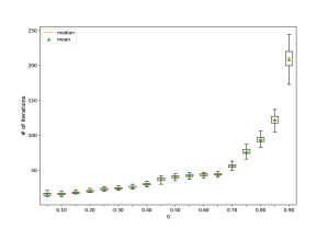
Figure 1: The effect of linear system solver error on the number of iterations of the self-dual embedding IF-IPM.

Fig. 1 illustrates how the noise of the linear system solver affects the number of iterations of the proposed self-dual embedding IF-IPM. The number of iterations of the algorithm increases as the error level increases. However, the algorithm is relatively stable with respect to $\eta$ while it is less than $0.7$. The number of iterations increases rapidly as the error parameter converges to $1$.

As the IF-IPM converges to the central optimal solution, the condition number of linear systems solved at every iteration of the algorithm grows to infinity. The largest condition number of the OSS occurs at the last iterations of IF-IPM. Fig. 2 shows how the largest condition number of the OSS changes in the self-dual IF-IPM with respect to different parameters of the problem and the algorithm. Fig. 2a indicates that the condition number of the OSS is almost indifferent to the smallest singular value of $A^{\prime}$. Here, we adjust the smallest singular value of the matrix $A^{\prime}$ by just changing its condition number while keeping its norm constant. In other words, the condition number of the OSS does not depend directly on the condition number of matrix $A^{\prime}$, which is one of its submatrices. Conversely, the largest singular values of OSS submatrices, i.e., the $\ell_{2}$ norm of those submatrices, affect the OSS condition number. Fig. 2b and Fig. 2d show that the norm of matrix $A^{\prime}$ and right-hand side (RHS) vector $b^{\prime}$ have a direct relationship with the condition number of the OSS. A similar trend can be observed with vector $c^{\prime}$. As shown in Fig. 2c, the condition number of the OSS changes with rate $\frac{1}{\zeta}$. This observation can be explained by the relationship derived in (17).

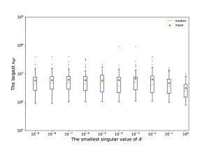
(a) The smallest singular value of matrix $A^{\prime}$

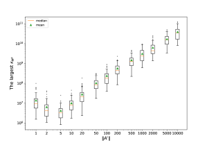
(b) The norm of matrix $A^{\prime}$

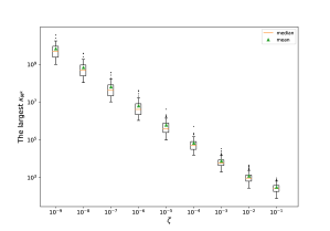
(c) The desired precision

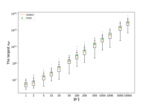
(d) The norm of RHS vector $b^{\prime}$

Figure 2: The effect of different properties on the largest condition number of the OSS in the self-dual embedding IF-IPM.

As we can see in Fig. 3 that the condition number of the OSS system is as good as the one for the full Newton system, and better than the Augmented system and Normal Equation system. Also, Figure 3c verifies that the condition number of the OSS system will go to infinity with rate $\frac{1}{\mu}$ in the worst case, which is better than the Augmented system and Normal Equation System. Figure 3d shows how Iterative Refinement can help to avoid the growing condition number of the Newton system. More precisely, by restarting QIPM in each iteration of IR, the algorithm starts with a system with relatively low condition number.

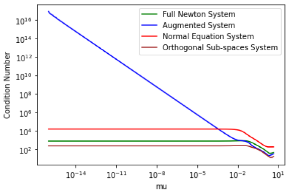
(a) Well-conditoned $A$

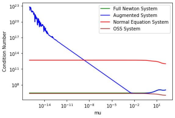
(b) Ill-conditoned $A$

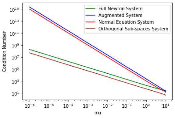
(c) Primal degenerate problem

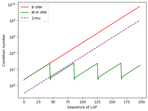
(d) Effect of Iterative Refinement

Figure 3: Iterations of IF-IPM with different levels of error.

9 Conclusion

Motivated by the efficient use of QLSA in IPMs, an Inexact Feasible IPM (IF-IPM) is developed with ${\cal O}(\sqrt{n}L)$ iteration complexity, analogous to the best exact feasible IPM. In terms of classical computing, as well as quantum computing, it is a novel algorithm. The improvement in total complexity comes from taking feasible steps using fast but inexact quantum or classical linear solvers. We proposed a new linear system, called Orthogonal Spaces System, to generate inexact but feasible Newton steps. In consequence, an Inexact Feasible Quantum IPM is developed to solve LO problems nearly as fast as the best classical IPMs. We analyzed the proposed IF-IPM theoretically and empirically. It is necessary to use an iterative refinement scheme to avoid exponential complexity for finding an exact optimal solution using IF-QIPM coupled with QLSAs or IF-IPM with CGMs.

Algorithm	Time Complexity
Best classical bound	${\cal O}(n^{3}L)$
QIPM of [19]	$\tilde{{\cal O}}_{n}\Big{(}n^{2}L\bar{\kappa}^{3}2^{4L}\Big{)}^{*}$
QIPM of [7]	$\tilde{{\cal O}}_{n}\big{(}n^{2}L\bar{\kappa}^{2}2^{2L}\big{)}^{*}$
IR-II-QIPM of [26]	$\tilde{{\cal O}}_{n,\omega,\kappa_{\hat{A}},\|\hat{A}\|,\|\hat{b}\|}\big{(}n^{4}L\kappa_{\hat{A}}^{3}\|\hat{A}\|^{2}\|\hat{b}\|\omega^{8}\big{)}$
IR-II-IPM + CGM of [26]	$\tilde{{\cal O}}_{\omega,\|\hat{A}\|,\|b\|}\big{(}n^{4}L\kappa_{\hat{A}}\omega^{2}\big{)}$
The proposed IR-IF-QIPM	$\tilde{{\cal O}}_{n,\kappa_{Q},\omega,\mu^{0},L}\big{(}n^{2.5}L\kappa_{Q}^{2}\|Q\|\omega^{5}\big{)}$
The proposed IR-IF-IPM + CGM	$\tilde{{\cal O}}_{\mu^{0},L}\big{(}n^{2.5}L\kappa_{Q}\omega^{2}\big{)}$

Table 2: Time complexity of finding the exact solution using different QIPMs ($*$ indicates the time complexity is not attainable)

Table 2 indicates that with respect to dimension the best theoretical bound for solving LO problems has been improved for the first time, but this complexity still depends on constants, such as $\kappa_{Q}$ and $\omega$. The proposed IR-IF-QIPM has much better time complexity than IR-II-QIPM for solving LO problems. The QIPMs proposed in [19, 7] seem to have a better dependence on $n$. However, their time complexities can not be attained since they are on the premises that QLSAs can provide an exact solution. This fundamental assumption invalidates the whole convergence of a QIPM algorithm since quantum algorithms are inherently noisy. All in all, the proposed IR-IF-QIPM has the best complexity among convergent QIPMs and w.r.t the dimension better complexity than classical IPMs.

Quantum algorithms particularly QLSAs have opened up a new avenue of research in solving optimization problems. They can be coupled with classical iterative methods to mitigate their inherent noise. Although this paper just studied an application of QLSAs, the proposed method takes advantage of the best iteration complexity of feasible IPMs and the low cost of iterative methods, such as CGM. The condition number of OSS is increasing more slowly than that of other Newton systems. We also employed an iterative refinement scheme using the proposed IF-QIPM with low precision to address both errors of QLSAs and the growing condition number of Newton systems. Another promising line of research is to study preconditioning and regularization techniques for the OSS to mitigate the impact of the growing condition number in IF-(Q)IPMs through iterative methods. This paper is the first comprehensive approach to develop an inexact but feasible IPMs to solve LO problems. This direction can be pursued by modifying the NES to guarantee the feasibility of the inexact solution but taking advantage of small positive definite coefficient matrices. The proposed IF-IPM can also be extended to other optimization problems, such as conic and nonlinear optimization problems.

References

• [1] G. Al-Jeiroudi and J. Gondzio, Convergence analysis of the inexact infeasible interior-point method for linear optimization, Journal of Optimization Theory and Applications, 141 (2009), pp. 231–247, https://doi.org/10.1007/s10957-008-9500-5.
• [2] E. D. Andersen, C. Roos, T. Terlaky, T. Trafalis, and J. P. Warners, The use of low-rank updates in interior-point methods, in Numerical Linear Algebra and Optimization, J. Y. Yuan, ed., Science Press, Beijing, China, 2004, pp. 3–14, https://bit.ly/3WM0Ly2.
• [3] B. Augustino, G. Nannicini, T. Terlaky, and L. Zuluaga, Solving the semidefinite relaxation of QUBOs in matrix multiplication time, and faster with a quantum computer, arXiv preprint arXiv:2301.04237, (2023).
• [4] B. Augustino, G. Nannicini, T. Terlaky, and L. F. Zuluaga, Quantum interior point methods for semidefinite optimization, arXiv preprint, (2021), https://doi.org/10.48550/arXiv.2112.06025.
• [5] V. Baryamureeba and T. Steihaug, On the convergence of an inexact primal-dual interior point method for linear programming, in Large-Scale Scientific Computing, I. Lirkov, S. Margenov, and J. Waśniewski, eds., Berlin, Heidelberg, 2006, Springer Berlin Heidelberg, pp. 629–637.
• [6] S. Bellavia, Inexact interior-point method, Journal of Optimization Theory and Applications, 96 (1998), pp. 109–121, https://doi.org/10.1023/A:1022663100715.
• [7] P. Casares and M. Martin-Delgado, A quantum interior-point predictor–corrector algorithm for linear programming, Journal of Physics A: Mathematical and Theoretical, 53 (2020), p. 445305, https://doi.org/10.1088/1751-8121/abb439.
• [8] S. Chakraborty, A. Gilyén, and S. Jeffery, The power of block-encoded matrix powers: improved regression techniques via faster Hamiltonian simulation, arXiv preprint arXiv:1804.01973, (2018).
• [9] A. M. Childs, R. Kothari, and R. D. Somma, Quantum algorithm for systems of linear equations with exponentially improved dependence on precision, SIAM Journal on Computing, 46 (2017), p. 1920–1950, https://doi.org/10.1137/16m1087072.
• [10] G. B. Dantzig, Linear Programming and Extensions, Princeton University Press, Princeton, NJ, USA, 1963, https://doi.org/10.1515/9781400884179.
• [11] D. Deutsch and R. Penrose, Quantum theory, the Church-Turing principle and the universal quantum computer, Proceedings of the Royal Society of London. A. Mathematical and Physical Sciences, 400 (1985), pp. 97–117, https://doi.org/10.1098/rspa.1985.0070.
• [12] E. Farhi, J. Goldstone, and S. Gutmann, A quantum approximate optimization algorithm, arXiv preprint, (2014), https://arxiv.org/abs/1411.4028.
• [13] R. W. Freund, F. Jarre, and S. Mizuno, Convergence of a class of inexact interior-point algorithms for linear programs, Mathematics of Operations Research, 24 (1999), pp. 50–71, https://doi.org/10.1287/moor.24.1.50.
• [14] J. Gondzio, Convergence analysis of an inexact feasible interior point method for convex quadratic programming, SIAM Journal on Optimization, 23 (2013), pp. 1510–1527.
• [15] L. K. Grover, A fast quantum mechanical algorithm for database search, in Proceedings of the Twenty-Eighth Annual ACM Symposium on Theory of Computing, Association for Computing Machinery, 1996, pp. 212–219, https://doi.org/10.1145/237814.237866.
• [16] A. W. Harrow, A. Hassidim, and S. Lloyd, Quantum algorithm for linear systems of equations, Physical Review Letters, 103 (2009), https://doi.org/10.1103/PhysRevLett.103.150502.
• [17] R. A. Horn and C. R. Johnson, Matrix Analysis, Cambridge University Press, 2012.
• [18] N. Karmarkar, A new polynomial-time algorithm for linear programming, in Proceedings of the Sixteenth Annual ACM Symposium on Theory of Computing, STOC ’84, New York, NY, USA, 1984, Association for Computing Machinery, p. 302–311, https://doi.org/10.1145/800057.808695.
• [19] I. Kerenidis and A. Prakash, A quantum interior point method for LPs and SDPs, ACM Transactions on Quantum Computing, 1 (2020), pp. 1–32, https://doi.org/10.1145/3406306.
• [20] L. G. Khachiyan, A polynomial algorithm in linear programming, Doklady Akademii Nauk, 244 (1979), pp. 1093–1096, http://mi.mathnet.ru/eng/dan42319.
• [21] V. Klee and G. J. Minty, How good is the simplex algorithm, Inequalities, 3 (1972), pp. 159–175, https://books.google.com/books?id=R843OAAACAAJ.
• [22] M. Kojima, N. Megiddo, and S. Mizuno, A primal—dual infeasible-interior-point algorithm for linear programming, Mathematical Programming, 61 (1993), pp. 263–280, https://doi.org/10.1007/BF01582151.
• [23] J. Korzak, Convergence analysis of inexact infeasible-interior-point algorithms for solving linear programming problems, SIAM Journal on Optimization, 11 (2000), pp. 133–148, https://doi.org/10.1137/S1052623497329993.
• [24] S. Mizuno and F. Jarre, Global and polynomial-time convergence of an infeasible-interior-point algorithm using inexact computation, Mathematical Programming, 84 (1999), pp. 105–122, https://doi.org/10.1007/s10107980020a.
• [25] M. Mohammadisiahroudi, R. Fakhimi, B. Augustino, and T. Terlaky, Generating linear, semidefinite, and second-order cone optimization problems for numerical experiments, arXiv preprint arXiv:2302.00711, (2023).
• [26] M. Mohammadisiahroudi, R. Fakhimi, and T. Terlaky, Efficient use of quantum linear system algorithms in interior point methods for linear optimization, arXiv preprint arXiv:2205.01220, (2022).
• [27] R. D. Monteiro and J. W. O’Neal, Convergence analysis of a long-step primal-dual infeasible interior-point LP algorithm based on iterative linear solvers, Georgia Institute of Technology, (2003), http://www.optimization-online.org/DB_FILE/2003/10/768.pdf.
• [28] G. Nannicini, Fast quantum subroutines for the simplex method, Operations Research, (2022).
• [29] C. Roos, T. Terlaky, and J.-P. Vial, Interior Point Methods for Linear Optimization, Springer Science & Business Media, 2005, https://doi.org/10.1007/b100325.
• [30] Y. Saad, Iterative Methods for Sparse Linear Systems, SIAM, 2003, https://doi.org/10.1137/1.9780898718003.
• [31] P. W. Shor, Algorithms for quantum computation: discrete logarithms and factoring, in Proceedings 35th Annual Symposium on Foundations of Computer Science, IEEE, 1994, pp. 124–134, https://doi.org/10.1109/SFCS.1994.365700.
• [32] T. Terlaky, Interior Point Methods of Mathematical Programming, vol. 5, Springer Science & Business Media, 2013, https://doi.org/10.1007/978-1-4613-3449-1.
• [33] J. van Apeldoorn, A. Cornelissen, A. Gilyén, and G. Nannicini, Quantum tomography using state-preparation unitaries, in Proceedings of the 2023 Annual ACM-SIAM Symposium on Discrete Algorithms (SODA), SIAM, 2023, pp. 1265–1318.
• [34] L. Wossnig, Z. Zhao, and A. Prakash, Quantum linear system algorithm for dense matrices, Physical Review Letters, 120 (2018), https://doi.org/10.1103/physrevlett.120.050502.
• [35] S. J. Wright, Primal-Dual Interior-Point Methods, SIAM, 1997, https://doi.org/10.1137/1.9781611971453.
• [36] Y. Ye, M. J. Todd, and S. Mizuno, An $O(\sqrt{n}L)$-iteration homogeneous and self-dual linear programming algorithm, Mathematics of Operations Research, 19 (1994), pp. 53–67, https://doi.org/10.1287/moor.19.1.53.
• [37] G. Zhou and K.-C. Toh, Polynomiality of an inexact infeasible interior point algorithm for semidefinite programming, Mathematical Programming, 99 (2004), pp. 261–282, https://doi.org/10.1007/s10107-003-0431-5.