Commuting Line Defects At $q^{N}=1$

Abstract

We explain the physical origin of a curious property of algebras ${\mathcal{A}}_{\mathfrak{q}}$ which encode the rotation-equivariant fusion ring of half-BPS line defects in four-dimensional ${\cal N}=2$ supersymmetric quantum field theories. These algebras are a quantization of the algebras of holomorphic functions on the three-dimensional Coulomb branch of the SQFTs, with deformation parameter $\log{\mathfrak{q}}$. They are known to acquire a large center, canonically isomorphic to the undeformed algebra, whenever ${\mathfrak{q}}$ is a root of unity. We give a physical explanation of this fact. We also generalize the construction to characterize the action of this center in the ${\mathcal{A}}_{\mathfrak{q}}$-modules associated to three-dimensional ${\cal N}=2$ boundary conditions. Finally, we use dualities to relate this construction to a construction in the Kapustin-Witten twist of four-dimensional ${\cal N}=4$ gauge theory. These considerations give simple physical explanations of certain properties of quantized skein algebras and cluster varieties, and quantum groups, when the deformation parameter is a root of unity.

1 Introduction

The quantization of a classical, finite-dimensional phase space is a subtle and ambiguous art qm1 ; qm2 ; qm3 . A typical challenge is to produce a quantization which preserves some desirable properties of the original classical system.

The study of supersymmetric quantum field theories has offered several novel ways to address such challenges Kontsevich:1997vb ; Kapustin:2001ij ; Kapustin:2005vs ; Gukov:2008ve ; Nekrasov:2009rc ; Nekrasov:2010ka ; Witten:2010zr ; Yagi:2014toa ; Bullimore:2015lsa ; Beem:2016cbd ; Pestun:2007rz ; Alday:2009fs ; Drukker:2009id ; Gaiotto:2010be ; Dimofte:2011py . The general idea is that protected quantities in certain SQFTs can be organized in the form of an auxiliary one-dimensional quantum mechanical system, whose properties are strongly constrained by the symmetries and dualities of the underlying field theory.

A typical scenario involves a one-parameter family of supersymmetric systems labelled by the quantization parameter $\hbar$, equipped with an algebra $A_{\hbar}$ of topological local operators which are bound to a line in space-time when $\hbar\neq 0$, but free to move away from the line when $\hbar=0$ Kontsevich:1997vb ; Gukov:2008ve ; Yagi:2014toa ; Bullimore:2015lsa ; Beem:2016cbd . The product of local operators bound to a line can be noncommutative, but must become commutative when operators can be moved off the line and switch position without colliding.

In this paper we consider a special situation where the algebra only depends on $\hbar$ through the exponential $q=\text{e}^{2\pi{\mathrm{i}}\hbar}$ Alday:2009fs ; Drukker:2009id ; Gaiotto:2010be ; Dimofte:2011py . In these situations we find that a subset of the local operators can move off the line for rational values of $\hbar$ other than $0$. This implies that the quantum algebra $A_{\hbar}$ develops a large center when $\hbar$ approaches these values, with properties controlled by the underlying physical system.

The prototypical example of this phenomenon occurs for the quantum torus algebra, generated by invertible elements $X$ and $P$ with

$$XP=qPX\,.$$ (1)

At $\hbar=0$, $X$ and $P$ generate the algebra of holomorphic functions on $\mathbb{C}^{*}\times\mathbb{C}^{*}$. Whenever $q$ is specialized to an $N$-th root of unity, i.e. $q^{N}=1$, then $X_{N}\equiv X^{N}$ and $P_{N}\equiv P^{N}$ become central. These central elements generate a commutative subalgebra, which can be canonically identified with the classical algebra, via the algebra morphism generated by $X_{\mathrm{cl}}\mapsto X_{N}$ and $P_{\mathrm{cl}}\mapsto P_{N}$.

This observation may appear rather trivial, but becomes more surprising if we consider a quantum cluster transformation such as

$$P\to(1-X)P$$ (2)

This transformation acts on the center in a remarkably simple manner:

$$P_{N}\to(1-X)P\cdots(1-X)P=(1-X)\cdots(1-q^{1-N}X)P_{N}=(1-X_{N})P_{N}\,,$$ (3)

which is identical to the classical limit of the cluster transformation.

Cluster varieties Fock:2003xxy are a large class of complex symplectic manifolds equipped with an atlas of $(\mathbb{C}^{*})^{d}$ coordinate patches related by cluster transformations. They can be quantized systematically by promoting the $(\mathbb{C}^{*})^{d}$ to quantum torus algebras and gluing them together via quantum cluster transformations. Parsing through the definitions specialized to $q^{N}=1$, one derives a very general result: the quantized algebra ${\cal A}_{q}$ of holomorphic functions on a cluster variety contains a large center if $q$ is a root of unity, which can be canonically identified with the classical algebra ${\cal A}_{1}$, simply by mapping classical cluster variables to the $N$-th power of the quantum cluster variables. This phenomenon was already pointed out in Fock:2003xxy , and has been explored in the physics literature e.g. Cecotti:2010fi .

A particularly important type of cluster variety is a character variety, aka moduli space of flat $G$-connections on a punctured Riemann surface $C$. In this case, the quantized algebra ${\cal A}_{q}$ has a local description on $C$, as a skein algebra of topological line defects in (analytically-continued) Chern-Simons theory. When ${\mathfrak{g}}$ is of type $A_{1}$, the appearance of a large center isomorphic to ${\mathcal{A}}_{1}$ when $q^{N}=1$ has been proved and used to study the representation theory, e.g. Bonahon_2015 ; Bonahon_2017 ; korinman2023classical ; MR3830231 . Another particularly important example of a quantized character variety is the quantized universal enveloping algebra ${\cal A}_{q}=U_{q}({\mathfrak{g}})$; there too, the appearance of a large center isomorphic to ${\mathcal{A}}_{1}$ when $q^{N}=1$ is a known and important phenomenon, e.g. MR1103601 ; MR1124981 ; BECK199429 .

In this paper we offer a simple and transparent physical explanation for this large-center phenomenon, for a particular class of algebras ${\mathcal{A}}_{q}$, namely those which can be defined through the Melvin compactification Melvin:1963qx ; Nekrasov:2003rj ; Hellerman:2012zf ; Gaiotto:2010be ; Braverman:2016wma of 4d ${\cal N}=2$ gauge theories. In the special case of theories of class ${\mathcal{S}}$, our description involves the Melvin compactifications of 6d $(2,0)$ theories, and can be re-expressed in the language of the Kapustin-Witten twist of 4d ${\cal N}=4$ gauge theories Kapustin:2006pk ; Gaiotto:2008sd ; Gaiotto:2008ak ; Gaiotto:2008sa ; Witten:2010cx ; Nekrasov:2010ka ; Witten:2011zz ; Gaiotto:2011nm . In either description, we explain how judicious configurations of supersymmetric defects both justify and extend the expected root-of-unity phenomena, and offer a variety of potential mathematical conjectures.

Our physics perspective is also relevant for a large class of of “$K_{2}$-Lagrangian” submanifolds Dimofte:2013iv ${\cal L}$ of cluster varieties, which are essentially built out of cluster transformations and have nice quantizations as modules ${\cal L}_{q}$ for ${\cal A}_{q}$. Such manifolds emerge naturally from 3d ${\cal N}=2$ boundary conditions of 4d ${\cal N}=2$ gauge theories Dimofte:2011py ; Beem:2012mb ; Dimofte:2013lba . They also arise in the context of character varieties, as spaces of flat connections and skein modules ${\cal L}_{q}$ associated to three-dimensional geometries with boundary $C$ Dimofte:2013lba . Our physics setup predicts a nice behaviour when $q$ is a root of unity: the center of ${\cal A}_{q}$ acting on ${\cal L}_{q}$ should satisfy the same relations as those defining the classical Lagrangian ${\cal L}$.

We conclude this introduction by mentioning just one of the original motivations for this work. The quantization of Coulomb branches of three-dimensional ${\cal N}=4$ SQFTs produces algebras $A_{\hbar}$ akin to the Weyl algebra (i.e. the universal enveloping algebra of the Heisenberg algebra defined by $[x,p]={\mathrm{i}}\hbar$) Yagi:2014toa ; Bullimore:2015lsa ; Beem:2016cbd ; Braverman:2016pwk ; Braverman:2016wma . In these examples one could scale $\hbar$ to $1$, and hence there cannot be root-of-unity phenomena. Instead, these quantized algebras can be defined in characteristic $p$ 2005math1247B and again have a large center which is canonically isomorphic to the classical algebra. This has been used to great effect 2019arXiv190504623W to study the properties of Coulomb branches, but a physical interpretation of characteristic $p$ calculations is missing.

In practice, the quantization in characteristic $p$ is employed to define interesting sheaves on 3d Coulomb branches. The root-of-unity setting in four dimensions can be used in the same manner to produce sheaves on 4d Coulomb branches, to which we can give a clear physical meaning. The 3d Coulomb branches are limits of 4d Coulomb branches. It would be interesting to compare the sheaves obtained by the two methods. For example, we claim that the 4d sheaves have a natural hyperholomorphic structure, and it would be interesting to know whether this structure persists into the 3d version.

2 The centers of algebras of line defects at roots of unity

2.1 Preliminaries on line defects

The main actors in our construction are half-BPS line defects in a four-dimensional ${\mathcal{N}}=2$ supersymmetric quantum field theory we denote as $T$. We refer to Gaiotto:2010be for a detailed discussion of the properties of such line defects and a physical derivation of the algebras ${\cal A}_{\mathfrak{q}}[T]$ associated to these line defects.

Many of the details of the physical definition of half-BPS line defects are actually unnecessary for this physical derivation. In particular, a physical defect may belong to a large deformation class of defects, which would be identified at the level of the algebra.

A more modern perspective would employ a holomorphic-topological (HT) twist of the physical theory, i.e. a twist which makes two directions of space-time topological and combines the remaining two in an holomorphic direction. See e.g. Aganagic:2017tvx ; Costello:2020ndc for a three-dimensional analogue. Supersymmetric line defects map under the twist to topological line defects wrapping one of the topological directions (e.g. “time”) and can be fused along the transverse topological direction.

Working equivariantly for the group $\operatorname{Spin}(2)$ of rotations of the holomorphic direction, such topological defects form a (derived) ${\mathbb{C}}^{*}$-equivariant monoidal category. The “collection of line defects” could be tentatively formalized as the K-theory of such a category. The construction of 2018arXiv180108111C should be understood as an example of such a construction.

In the following we will write formulae assuming the existence of some countable collection of linear generators ${\mathfrak{L}}_{i}$ for the K-theory, so that the fusion of (classes of) line defects will be a direct sum of (classes of) line defects with coefficients which are K-theory classes of “Chan-Paton” vector spaces, which may carry quantum numbers for the symmetries of the problem:

$${\mathfrak{L}}_{i}\,{\mathfrak{L}}_{j}=\bigoplus_{k}[V^{k}_{ij}]\otimes{\mathfrak{L}}_{k}\,.$$ (4)

The language of K-theory is particularly useful in the context of $S^{1}$ compactifications of the theory. Line defects wrapping $S^{1}$ appear as local operators in the three-dimensional effective field theory, which only depend on the K-theory class of the original line. Relations such as (4) capture the product of these 3d local operators, while making manifest integrality properties inherited from the underlying 4d setup: the 3d structure constants in this basis will be expressed as characters of the $[V^{k}_{ij}]$. We will come back to this momentarily in subsection 2.2.

We will not employ the language of twisted SQFT in the rest of this paper, but a translation should be straightforward (and would likely streamline our arguments). Constructions involving six-dimensional $(2,0)$ SCFTs should be analogously recast in terms of their HT twist.

The Melvin space $M_{q}$ is the simplest non-trivial three-dimensional “HT” geometry, i.e. a manifold equipped with a transverse holomorphic foliation Aganagic:2017tvx . A four-dimensional HT theory can thus be defined on $\mathbb{R}\times M_{q}$. This is the context where ${\mathcal{A}}_{\mathfrak{q}}$ will arise.

In the physical theory, it is natural to consider line operators which are equivariant under the $\operatorname{Spin}(3)$ group of rotations. However, both the HT twist and the operation of fusion are only compatible with equivariance under the $\operatorname{Spin}(2)$ subgroup fixing the topological fusion direction. It would be interesting to find criteria to pin down K-theory classes which include $\operatorname{Spin}(3)$-equivariant defects. We suspect they would generate the collection in an appropriate sense; this conjecture could have interesting mathematical consequences, but we will not study it in this paper.

2.2 Line defects and local operators

The four-dimensional SQFT $T$ can be compactified on a circle with Ramond spin structure while preserving all supercharges. The resulting effective three-dimensional ${\mathcal{N}}=4$ SQFT has a Coulomb branch of vacua. Upon choosing a parameter $\zeta\in{\mathbb{C}}^{*}$, we can identify this Coulomb branch as a complex symplectic manifold ${\mathcal{M}}_{-}[T]$, which parameterizes the expectation values of half-BPS line defects wrapping the internal circle. Throughout this paper we will hold $\zeta$ fixed — say, to $\zeta=1$ — and not consider the extra structure coming from varying this choice (with one brief exception, in subsection 2.7.) As a complex symplectic manifold, ${\mathcal{M}}_{-}[T]$ has a weak dependence on the radius $R$ of the circle: a change of radius can be absorbed in a rescaling of the dimensionful parameters of $T$ (if any). Thus we will generally hold $R=1$, except in a few places where we consider the limit of small $R$.

We denote as ${\cal A}_{-}[T]$ the Poisson algebra generated by the half-BPS line defects wrapping the internal circle. This commutative algebra has integral structure constants (“fusion coefficients”) which capture coarse information about the fusion of line defects. If we denote as $L_{i}$ the local operator obtained by circle-wrapping ${\mathfrak{L}}_{i}$, the algebra takes the form

$$L_{i}L_{j}=\sum_{k}n^{k}_{ij}L_{k}\,.$$ (5)

By taking expectation values we can identify ${\mathcal{A}}_{-}[T]$ with the algebra of global holomorphic functions on ${\mathcal{M}}_{-}[T]$, and under this identification the product in (5) is the usual product of functions.

The circle compactification can be twisted by holonomies for every “flavour” symmetry of the theory, i.e. every global symmetry which commutes with the supercharges. This gives commutative deformations of ${\mathcal{A}}_{-}[T]$, as the fusion coefficients in the algebra are replaced by characters of fusion spaces, which are Laurent polynomials in appropriate fugacities $\mu$ for the flavour symmetries:

$$L_{i}L_{j}=\sum_{k,f}n^{k}_{ij}[f]\mu^{f}L_{k}$$ (6)

This is the algebra of functions on “mass deformations” of the 3d Coulomb branch, with $\mu$ being combinations of masses and flavour holonomies. Whenever we refer to ${\mathcal{A}}_{-}[T]$, ${\mathcal{M}}_{-}[T]$ etc. below we will include the possibility of such deformations.

All 4d ${\mathcal{N}}=2$ theories which we will discuss are equipped with an $SU(2)_{R}$ R-symmetry. The $\mathbb{Z}_{2}$ diagonal combination of the centers $(-1)^{F}$ and $(-1)^{R}$ of the centers of the $\operatorname{Spin}(3)$ rotation group and of $SU(2)_{R}$ commutes with the supercharges and is always available to twist the circle compactification. The result is another 3d Coulomb branch ${\mathcal{M}}_{+}[T]$ and Poisson algebra of functions ${\cal A}_{+}[T]$.

In order to “quantize” the Poisson algebras ${\cal A}_{\pm}[T]$, we can further refine the characters of fusion spaces by a fugacity ${\mathfrak{q}}$ for a certain combination of $\operatorname{Spin}(3)$ and $SU(2)_{R}$. This is best formulated in terms of a Melvin compactification of the theory, which we now introduce.

2.3 The Melvin compactification

Fix $q\in{\mathbb{C}}^{\times}$ with $\lvert q\rvert=1$. We consider the 4d Euclidean spacetime

$${{\mathbb{R}}}\times M_{q}\,,$$

where ${{\mathbb{R}}}$ is coordinatized by $t$, and $M_{q}$ is the Melvin space defined by

$$M_{q}=\{(z,x)\in{\mathbb{C}}\times{{\mathbb{R}}}\}\,/\,[(z,x)\sim(qz,x+1)]\,.$$ (7)

We collect here a few preliminary comments on the topology and geometry of $M_{q}$, which will be useful in our subsequent discussion. There is a natural projection $\pi:M_{q}\to S^{1}$, defined by $\pi([z,x]):=[x]$. Each fiber of this projection is $\mathbb{C}$. The resulting bundle has structure group $\operatorname{SO}(2)$ and a natural flat connection with holonomy $R_{q}:z\mapsto qz$. There is also a natural section $\psi:S^{1}\to M_{q}$ defined by $\psi([x]):=[(0,x)]$. The image of $\psi$ is a closed loop in $M_{q}$, whose homotopy class generates $\pi_{1}(M_{q})\simeq\mathbb{Z}$.

When $q$ is a primitive $N^{\mathrm{th}}$ root of unity, the covering map $\mathbb{C}\times\mathbb{R}\to M_{q}$ generated by the deck transformation $\phi_{q}:(z,x)\mapsto(qz,x+1)$ factors through

$$\mathbb{C}\times\mathbb{R}\to\mathbb{C}\times\tilde{S}^{1}\to M_{q}\,,$$ (8)

where the first map has deck group $\mathbb{Z}$ generated by $\phi_{q}^{N}$, and the second is a smooth $N$-fold covering. Here $\tilde{S}^{1}$ is a circle, best thought of as the quotient of $\mathbb{R}$ by $x\mapsto x+N$. In this case, for every $z_{0}\in\mathbb{C}$ there is a map $\psi_{z_{0}}:S^{1}\to M_{q}$ defined by $\psi_{z_{0}}([x]):=[(z_{0},Nx)]$. The image of $\psi_{z_{0}}$ is a loop in $M_{q}$ which lifts to a closed loop in $\mathbb{C}\times\tilde{S}^{1}$ and has a homotopy class which is $N$ times a generator of $\pi_{1}(M_{q})$. Indeed $(\psi_{z_{0}})_{*}\pi_{*}:\pi_{1}(S^{1})\to\pi_{1}(S^{1})$ is multiplication by $N$. For $z_{0}\not=0$, the intersection of this loop with the fiber of $\pi$ above any point $[x]$ is the orbit of $z_{0}$ under the $\mathbb{Z}_{N}$-action generated by $R_{q}$. See subsection 2.4 below.

$M_{q}$ has several useful geometric structures. First, since $R_{q}\in\operatorname{SO}(2)$ the deck transformation $\phi_{q}$ is an isometry of the Euclidean metric, which thus descends to a flat metric on $M_{q}$. Second, there is an action of ${\mathbb{R}}$ on $M_{q}$ by $[(z,x)]\mapsto[(z,x+s)]$, whose orbits give a foliation of $M_{q}$ with $1$-dimensional leaves; this is a transverse holomorphic foliation in the sense of Aganagic:2017tvx . The loops we discussed above are compatible with these geometric structures; indeed, for every $q$ with $|q|=1$, the image of $\psi$ is a compact geodesic, and also a compact leaf of the foliation; similarly, when $q$ is an $N^{\mathrm{th}}$ root of unity, the image of $\psi_{z_{0}}$, for any $z_{0}$, is also a compact geodesic and a compact leaf of the HT foliation.

The manifolds $M_{q}$ are all diffeomorphic to $\mathbb{C}\times S^{1}$ because a diffeomorphism of $\mathbb{C}\times\mathbb{R}$ of the form $f:(z,x)\to(ze^{ax},x)$ conjugates any $\phi_{q}$ to $\phi_{1}$. But these diffeomorphisms are not isometries, and, more to the point, do not preserve the HT structure. (See section 2 of Aganagic:2017tvx .) As HT geometries the $M_{q}$ are all inequivalent for different $q$.

To define the compactification of our ${\mathcal{N}}=2$ theory on ${{\mathbb{R}}}\times M_{q}$, we need to choose a spin structure. Recall that the set of spin structures on $M_{q}$ is a torsor for $H^{1}(M_{q},\mathbb{Z}_{2})\simeq\mathbb{Z}_{2}$. Choosing a spin structure is equivalent to choosing a lift of $R_{q}=q^{J_{3}}$ from $\operatorname{SO}(2)\subset\operatorname{SO}(3)$ to the double cover $\operatorname{Spin}(3)\simeq\operatorname{SU}(2)$. Here $J_{3}$ is a generator of $SU(2)$ normalized so that the eigenvalues of $2J_{3}$ in the fundamental representation are $\{\pm 1\}$. Such a choice can be written as $\tilde{R}_{\mathfrak{q}}=(-{\mathfrak{q}})^{2J_{3}}$ where ${\mathfrak{q}}^{2}=q$. The two choices of ${\mathfrak{q}}$ correspond to the two possible spin structures.

When ${\mathfrak{q}}\neq-1$, the theory on ${{\mathbb{R}}}\times M_{q}$ is not supersymmetric unless we include a flat background $\operatorname{SU}(2)_{R}$-connection on $M_{q}$. This background connection is classified by its holonomy around $S^{1}$. We choose this holonomy to be $(-{\mathfrak{q}})^{2I_{3}}$, where $I_{3}$ is a generator of $SU(2)_{R}$, normalized as above.

With these choices, for generic $q$, the theory on ${{\mathbb{R}}}\times M_{q}$ preserves the $4$ supercharges with $I_{3}+J_{3}=0$. In the exceptional case $q=1$ we have $M_{q}=M_{1}={\mathbb{C}}\times S^{1}$, so putting our theory on $M_{q}$ just means compactifying it on a circle as in subsection 2.2. In that case ${\mathfrak{q}}=-1$ is the case of trivial $\tilde{R}_{\mathfrak{q}}$, which corresponds to Ramond (periodic) spin structure and no $\operatorname{SU}(2)_{R}$ twist, while ${\mathfrak{q}}=+1$ corresponds to Neveu-Schwarz (antiperiodic) spin structure and a twist by $-1\in\operatorname{SU}(2)_{R}$. Thus the choice of ${\mathfrak{q}}=\pm 1$ leads to the algebras ${\mathcal{A}}_{\pm}[T]$ which we discussed in subsection 2.2.

When $q\neq 1$ is a root of unity we only have $4$ supercharges, just as for generic $q$. Nevertheless, the root of unity case turns out to have special features, as we discuss in the next section.

2.4 Line defects in the Melvin background

Now we consider placing supersymmetric line defects in ${{\mathbb{R}}}\times M_{q}$. Each line defect will be placed at a point $t\in{{\mathbb{R}}}$ and extended along a circle in $M_{q}$. In order for the line defect to be supersymmetric, this circle must be a closed Euclidean geodesic in $M_{q}$, i.e. locally a straight line.

When $q\neq 1$ is generic, the only closed Euclidean geodesic in $M_{q}$ is the one located at $z=0$, i.e. the image of $\psi:S^{1}\to M_{q}$ discussed in the previous section. Thus the space of possible insertion locations for the line defects is ${{\mathbb{R}}}_{t}$. The (K-theory classes of) line defects can be fused along the ${{\mathbb{R}}}_{t}$ direction to give an algebra ${\mathcal{A}}_{\mathfrak{q}}[T]$, whose structure coefficients are Laurent polynomials in ${\mathfrak{q}}$ with integer coefficients:

$$L_{i}L_{j}=\sum_{k,s}n^{k}_{ij}[s]{\mathfrak{q}}^{s}L_{k}\,.$$ (9)

The parameter ${\mathfrak{q}}$ plays the role of the fugacity for the combination of spin and R-symmetry rotations. The algebra ${\mathcal{A}}_{\mathfrak{q}}[T]$ is typically not commutative, as wrapped lines cannot exchange their position in ${{\mathbb{R}}}_{t}$ without colliding with each other.

In the $q\to 1$ limit, we recover the commutative algebras ${\mathcal{A}}_{\pm}[T]$. From the geometric perspective, this commutativity arises because we now have closed geodesics at any value $z=z_{0}$, and thus wrapped line defects can be moved away from $z=0$ to exchange their position in ${{\mathbb{R}}}_{t}$ without colliding with each other.

It is also interesting to consider the behavior near $q=1$. One geometric way to realize this is as follows. We rescale the metric in $M_{q}$ by a factor of $R$, so that the geodesic at $z=0$ now has length $R$. Next we set $q={\mathrm{e}}^{2\pi{\mathrm{i}}R\hbar}$, and take $R\to 0$ while holding $\hbar$ fixed. In that limit we are effectively reduced to a 3-dimensional ${\cal N}=4$ theory on ${{\mathbb{R}}}^{3}$, in $\Omega$-background Moore:1997dj ; Moore:1998et ; Nekrasov:2002qd , with $\hbar$ playing the role of the $\Omega$-background parameter. The wrapped line defects reduce to local operators of the ${\cal N}=4$ theory, and their commutator gives a deformation quantization of a naturally-defined Poisson bracket in ${\mathcal{A}}_{\pm}[T]$ (see e.g. Yagi:2014toa and Section 6 of Beem:2018fng ).

Our description in terms of four-dimensional field theory on $M_{q}$ extends this deformation quantization, and shows that the integrality properties of ${\mathcal{A}}_{\pm}$ survive quantization, leading to Laurent polynomials in ${\mathfrak{q}}$.

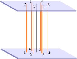
Figure 1: A multiwrapped line defect in $M_{q}$, in the case $N=6$, $q=\text{e}^{2\pi{\mathrm{i}}/6}$. The black segment is the circle $z=0$, while the orange segments are pieces of the multiwrapped defect. The two planes are identified by a rotation $z\mapsto qz$. After this identification the orange segments fit together into a single circle, which is a closed geodesic in $M_{q}$.

Now suppose $q$ is a primitive $N$-th root of unity, i.e. $q=\text{e}^{2\pi{\mathrm{i}}\frac{m}{N}}$ with $(m,N)=1$. In this case, as we remarked above, something special happens: we have again a continuous family of supersymmetric embeddings for a line defect, given by the loops $\psi_{z_{0}}$ in $M_{q}$ for any $z_{0}\in{\mathbb{C}}$. This is illustrated in subsection 2.4 for the example of $N=6$. Thus, any given line defect ${\mathfrak{L}}$ can be wrapped either on the core circle at $z=0$ to give an element $L_{\mathfrak{L}}$ of ${\mathcal{A}}_{\mathfrak{q}}$, or can be multiwrapped at a generic $z=z_{0}$.

Crucially, we can deform the multiwrapped line defect by bringing $z_{0}\to 0$. The result will not be $L_{\mathfrak{L}}$! Instead, it will be some other element $L_{\mathfrak{L},N}$ in ${\mathcal{A}}_{\mathfrak{q}}$, which is central: it can be deformed back to generic $z_{0}$ and moved across any other generator in ${\mathcal{A}}_{\mathfrak{q}}$.

Now let us discuss the fusion of the multiwrapped line defects. Each of the geodesics $\psi_{z_{0}}$ has an open neighborhood of the form $U\times{{\mathbb{R}}}\times\tilde{S}^{1}$, where $U$ is a disc in ${{\mathbb{R}}}^{2}$. Moreover, if we have two multiwrapped line defects on nearby geodesics $\psi_{z_{0}}$, $\psi_{z^{\prime}_{0}}$, we can find a single neighborhood $U\times{{\mathbb{R}}}\times\tilde{S}^{1}$ containing both of them. Since this neighborhood is isometric to an open subset in ${{\mathbb{R}}}^{3}\times\tilde{S}^{1}$, the fusion product of these line defects will be the same as the fusion product of line defects in ${{\mathbb{R}}}^{3}\times\tilde{S}^{1}$.

We need to discuss a detail concerning signs. As we have discussed in subsection 2.3, there are two possible ways of making the theory supersymmetric in ${{\mathbb{R}}}^{3}\times\tilde{S}^{1}$, labeled by a parameter $\tilde{\mathfrak{q}}=\pm 1$: around $\tilde{S}^{1}$ we take $SU(2)_{R}$ holonomy $-\tilde{\mathfrak{q}}$ and a spin structure which is Ramond if $\tilde{\mathfrak{q}}=-1$ and NS if $\tilde{\mathfrak{q}}=1$. What is the value of $\tilde{\mathfrak{q}}$ which actually occurs in our setup? Since $\tilde{S}^{1}$ is homologous to $N$ times $S^{1}$, the $SU(2)_{R}$ holonomy around $\tilde{S}^{1}$ is $(-{\mathfrak{q}})^{N}$; it follows that

$$-\tilde{\mathfrak{q}}=(-{\mathfrak{q}})^{N}\,.$$ (12)

For later convenience we rewrite this slightly: when $q$ is a primitive $N$-th root of unity, $(-{\mathfrak{q}})^{N}=-{\mathfrak{q}}^{N^{2}}\in\{\pm 1\}$ both for $N$ even and odd, and thus (12) becomes

$$\tilde{\mathfrak{q}}={\mathfrak{q}}^{N^{2}}\,.$$ (13)

Altogether, then, we conclude that the fusion algebra of the multiwrapped line defects is the commutative algebra ${\mathcal{A}}_{\pm}$, where the sign $\pm 1=\tilde{\mathfrak{q}}={\mathfrak{q}}^{N^{2}}$.

We now make an important assumption, that the K-theory class of the multi-wrapped ${\mathfrak{L}}$ defect only depends on the K-theory class of the circle-wrapped defect $L_{\mathfrak{L}}$. Under this assumption, we can define a homomorphism of algebras

$${\mathcal{A}}_{\pm}\to{\mathcal{A}}_{\mathfrak{q}}$$ (14)

by

$$L_{\mathfrak{L}}[\tilde{{\mathfrak{q}}}=\pm 1]\mapsto L_{\mathfrak{L},N}[{\mathfrak{q}}]\,.$$ (15)

We call this the multiwrapping map. Its image is central in ${\mathcal{A}}_{\mathfrak{q}}$.

How complicated should the multiwrapping map be in practice? A powerful principle is that the answer is independent of the coupling, and thus the calculation can be done in the most convenient duality frame. In particular, for Wilson line defects in gauge theories we can get good control by working at weak gauge coupling. This kind of argument has been used to predict that Wilson lines should fuse according to the tensor products of their respective representations:

$$L_{{\mathfrak{W}}[R]}L_{{\mathfrak{W}}[R^{\prime}]}=L_{{\mathfrak{W}}[R\otimes R^{\prime}]}$$ (16)

where ${\mathfrak{W}}[R]$ is a Wilson line in representation $R$. In a similar spirit, we conjecture (and verify below in examples) that in $G$ gauge theory we have

$$L_{{\mathfrak{W}}[R],N}=L_{{\mathfrak{W}}[\psi^{N}(R)]}\,,$$ (17)

where $\psi^{N}$ is an Adams operation on the K-theory of the category of $G$-representations, which literally encodes the concept of a multi-wrapped Wilson line:

$$\operatorname{Tr}_{\psi^{N}(R)}(g)=\operatorname{Tr}_{R}(g^{N})\,.$$ (18)

2.5 Line defects in the IR and Seiberg-Witten theory

At generic points $u$ of the 4d Coulomb branch, the theory $T$ admits a low-energy effective description in the form of an abelian gauge theory. Any BPS line defect ${\mathfrak{L}}$ also admits an effective description in terms of abelian line defects $\mathfrak{X}_{\gamma}$ with gauge and flavour charges $\gamma$. The qualifications we made in subsection 2.1 apply here: rather than the full physical line defects, at best we can discuss K-theory classes in some category of topological line defects in a twist of the theory. With this understood we write the UV-IR map as

$${\mathfrak{L}}\quad\rightsquigarrow\quad\bigoplus_{\gamma}\left[V_{{\mathfrak{L}},\gamma}\right]\otimes\mathfrak{X}_{\gamma}$$ (19)

where $V_{{\mathfrak{L}},\gamma}$ are (perhaps virtual) Chan-Paton vector spaces.

The framed BPS degeneracies introduced in Gaiotto:2010be agree with the characters of these Chan-Paton vector spaces,

$$\overline{\underline{\Omega}}(\mathfrak{L},\gamma,{\mathfrak{q}})={\rm Tr}_{V_{{\mathfrak{L}},\gamma}}(-1)^{2J_{3}}(-{\mathfrak{q}})^{2I_{3}+2J_{3}}\,.$$ (20)

These framed BPS degeneracies jump at walls of framed marginal stability in the Coulomb branch. Accordingly, the IR line defects ${\mathfrak{X}}_{\gamma}$ also jump, by cluster-like transformations controlled by the BPS spectrum of the theory.

As we did in subsection 2.4, we can wrap the IR line defects ${\mathfrak{X}}_{\gamma}$ around the core circle $\psi_{0}$, thus obtaining generators $X_{\gamma}:=L_{{\mathfrak{X}}_{\gamma}}$ of a noncommutative algebra ${\mathcal{A}}^{\mathrm{IR}}_{\mathfrak{q}}$ of local operators on the line. Moreover, ${\mathcal{A}}^{\mathrm{IR}}_{\mathfrak{q}}$ can be described explicitly: it is the quantum torus Gaiotto:2010be

$$X_{\gamma}X_{\gamma^{\prime}}={\mathfrak{q}}^{\langle\gamma,\gamma^{\prime}\rangle}X_{\gamma+\gamma^{\prime}}\,.$$ (21)

The fusion of line defects commutes with the flow from UV to IR; thus this flow gives a homomorphism ${\mathcal{A}}_{\mathfrak{q}}\to{\mathcal{A}}^{\mathrm{IR}}_{\mathfrak{q}}$.

All of our arguments about the multiwrapping map apply just as well in the IR theory as in the UV theory. Moreover, since the IR theory is an abelian gauge theory, and any IR line defect is a Wilson line in some duality frame, we can determine the multiwrapping map ${\mathcal{A}}^{\mathrm{IR}}_{\pm 1}\to{\mathcal{A}}^{\mathrm{IR}}_{\mathfrak{q}}$ completely using the Adams operations: indeed (17) just becomes

$$X_{\gamma,N}=X_{N\gamma}\,.$$ (22)

Now we can make a consistency check: we see directly from the quantum torus relation (21) that $X_{N\gamma}$ is central and

$$X_{N\gamma}X_{N\gamma^{\prime}}={\mathfrak{q}}^{N^{2}\langle\gamma,\gamma^{\prime}\rangle}X_{N(\gamma+\gamma^{\prime})}\,,$$ (23)

so the multiwrapped line defects indeed obey the relations of ${\mathcal{A}}^{\mathrm{IR}}_{\pm 1}$, with the sign $\pm 1={\mathfrak{q}}^{N^{2}}$ which we derived from the holonomy of the R-symmetry connection in subsection 2.4.

As we have already remarked, the local geometry around the multiwrapped defects is precisely the same as for the singly-wrapped defects. Moreover, the UV-IR map can be computed using only the local geometry around the defect and the constant vevs of Coulomb branch scalars of the 4d theory. It follows that the UV-IR map commutes with the multiwrapping map. Thus, given a wrapped line defect $L$ (arising as $L=L_{\mathfrak{L}}$ for some ${\mathfrak{L}}$), we may compute its multiwrapped image $L_{N}$ by first flowing to the IR and then applying the simple rule (22) to each IR summand. To summarize: if in some chamber $L$ has the IR expansion

$$L^{\mathrm{IR}}=\sum_{\gamma}c_{\gamma}[L,{\mathfrak{q}}]X_{\gamma}\,,$$ (24)

then the image of $L$ under the multiwrapping map defined in subsection 2.4 has IR expansion

$$L_{N}^{\mathrm{IR}}=\sum_{\gamma}c_{\gamma}[L,{\mathfrak{q}}^{N^{2}}]X_{N\gamma}\,.$$ (25)

This is the main result of this section: it gives a simple way of computing $L^{\mathrm{IR}}_{N}$ in terms of $L^{\mathrm{IR}}$.

We should observe that for gauge theories, the IR image of a non-abelian Wilson line is typically not a direct sum of abelian Wilson lines. The compatibility between our IR and UV predictions for multi-wrapped Wilson lines thus appears to impose strong constraints on the possible framed BPS spectra of non-abelian Wilson lines. We will explore this phenomenon in examples.

Setting aside the physical discussion for a moment, suppose we regard the right side of (25) as the definition of an object $L_{N}^{\mathrm{IR}}$. Then it is easy to see that the composite map $L[{\mathfrak{q}}^{N^{2}}]\mapsto L^{\mathrm{IR}}[{\mathfrak{q}}^{N^{2}}]\mapsto L^{\mathrm{IR}}_{N}$ is a homomorphism ${\mathcal{A}}_{{\mathfrak{q}}^{N^{2}}}\to{\mathcal{A}}^{\mathrm{IR}}_{\mathfrak{q}}$, with central image. What is not obvious is that $L^{\mathrm{IR}}_{N}$ so defined is actually the IR image of an element $L_{N}\in{\mathcal{A}}_{\mathfrak{q}}$. Nevertheless, this follows from our physical construction of $L_{N}$ in terms of multiwrapping line defects.

It also follows from this construction that (25) must be consistent with framed wall-crossing. This requires the quantum wall-crossing transformation of $X_{N\gamma}$ to match the classical wall-crossing transformation of $X_{\gamma}$. This is indeed the case, in a rather non-trivial manner. Indeed, in general, a quantum wall-crossing transformation multiplies $X_{\gamma}$ by products of factors of the form

$$\prod_{s=1}^{\langle\gamma^{\prime},\gamma\rangle}(1-(-{\mathfrak{q}})^{m}q^{-s}X_{\gamma^{\prime}})$$ (26)

or analogous ones depending on certain signs ks1 ; Gaiotto:2010be . If we make the replacement $\gamma\to N\gamma$, the product (26) becomes

$$\prod_{s=1}^{N\langle\gamma^{\prime},\gamma\rangle}(1-(-{\mathfrak{q}})^{m}q^{-s}X_{\gamma^{\prime}})\,,$$ (27)

which telescopes nicely to

$$(1-(-{\mathfrak{q}})^{Nm}X_{N\gamma^{\prime}})^{\langle\gamma^{\prime},\gamma\rangle}\,,$$ (28)

giving the expected classical wall-crossing transformation with sign ${\mathfrak{q}}^{N^{2}}$.

We conclude that different choices of IR chamber give equivalent definitions of $L_{N}$. This means, in particular, that we can try to check our claim that $L_{N}$ belongs to ${\mathcal{A}}_{\mathfrak{q}}$ by going to a convenient IR chamber.

The simplest possibility is that in some chamber we have $L=X$, for some $X=X_{\gamma}$ (i.e., in this chamber the line defect supports only a single framed BPS state). Then we see immediately that

$$L_{N}=L^{N}\,.$$ (29)

The relation (29) then holds universally, independent of a choice of chamber. In particular, it implies that $L_{N}$ is in ${\mathcal{A}}_{\mathfrak{q}}$ as expected, since $L$ is.

A more interesting example occurs in $A_{1}$ theories of class ${\cal S}$. In these theories, many line defects can be expanded as

$$L=X+X^{-1}$$ (30)

in specific chambers, matching their description as Wilson lines in a weakly-coupled $SU(2)$ gauge theory. Then (25) gives $L_{N}=X^{N}+X^{-N}$, and thus

$$L_{N}=2T_{N}(L/2)$$ (31)

where $T_{N}$ are Chebyshev polynomials of the first kind. For instance, $L_{2}=L^{2}-2$, and $L_{3}=L^{3}-3L$.

It follows from (31) that $L_{N}$ defined by (25) indeed lies in ${\mathcal{A}}_{\mathfrak{q}}$, as desired. Thus we recover a fact proven by different means in Bonahon_2015 : the root-of-unity quantization of $A_{1}$ character varieties has a large center generated by the elements $L_{N}=2T_{N}(L/2)$. We note also that (31) matches the expected (17).

This discussion generalizes to all line defects $L$ which can be realized as UV Wilson lines in some duality frame: one can typically define a weakly-coupled IR chamber where the Wilson lines $L$ are identified with Weyl-invariant polynomials in electric Darboux variables, and their multiwrappings $L_{N}$ can be identified as other linear combinations of Wilson lines, just as predicted by (17). We will exhibit some explicit examples in $A_{1}$ and $A_{2}$ theories in subsection 3.3 below.

We find it remarkable that the multiwrapping map $L\mapsto L_{N}$ encodes properties of line defects in a manner which is independent of the duality frame or IR chamber. It would be tempting to try to classify line defects according to how multiwrapping acts on them. For instance, we could call a line defect “pure” if it has $L_{N}=L^{N}$. (We have seen above that this is the case for any line defect which has a single framed BPS state in some chamber, but we stress that the property of being pure is a UV property, independent of any particular chamber.) More generally we could consider, for example, the class of line defects which have $L_{N}=F_{N}(L)$ for some polynomial function $F_{N}$.

2.6 Line defects on the boundary

We can also equip the 4d ${\mathcal{N}}=2$ theory $T$ with a half-BPS boundary condition $B$. Such a boundary condition supports a collection of BPS line defects, which can fuse with each other along the boundary, and also fuse with bulk line defects brought to the boundary. We now repeat all of our earlier constructions in the presence of the boundary.

First, we can consider $T$ on $[0,\infty)_{t}\times{{\mathbb{R}}}^{2}\times S^{1}$, with the boundary condition $B$ at $\{t=0\}\times{{\mathbb{R}}}^{2}\times S^{1}$. Then wrapping boundary line defects on $S^{1}$ gives operators which are free to move in the boundary ${{\mathbb{R}}}^{2}$, and thus form a commutative algebra ${\mathcal{L}}_{\pm}$. The algebra ${\mathcal{L}}_{\pm}$ is also acted on by ${\mathcal{A}}_{\pm}$, since the wrapped line defects in the bulk can fuse with the wrapped line defects on the boundary.

Let us discuss the structure of ${\mathcal{L}}_{\pm}$ as a module over ${\mathcal{A}}_{\pm}$. Given a point $x\in{\mathcal{M}}_{\pm}$ with corresponding maximal ideal $I_{x}\subset{\mathcal{A}}_{\pm}$, we can consider the quotient algebra ${\mathcal{L}}_{\pm}/I_{x}{\mathcal{L}}_{\pm}$; letting $x$ vary this gives a sheaf of quotient algebras over ${\mathcal{M}}_{\pm}[T]$. What can we say about this sheaf? Physically, the boundary condition $B$ descends to a boundary condition for the 3d theory, preserving 2d $(2,2)$ supersymmetry. Such a boundary condition should be supported on some complex Lagrangian submanifold ${\mathcal{M}}_{\pm}[B]$ of the 3d Coulomb branch ${\mathcal{M}}_{\pm}[T]$, consisting of the 3d vacua compatible with the boundary. We thus expect the sheaf representing ${\mathcal{L}}_{\pm}$ to be supported on ${\mathcal{M}}_{\pm}[B]\subset{\mathcal{M}}_{\pm}[T]$.

We can now “quantize” ${\mathcal{L}}_{\pm}$, by placing $T$ on $[0,\infty)_{t}\times M_{q}$, with the half-BPS boundary condition $B$ at $\{t=0\}\times M_{q}$. Boundary line defects wrapping the core circle at $z=0$ in $M_{q}$ form an ${\mathcal{A}}_{\mathfrak{q}}$-module ${\mathcal{L}}_{\mathfrak{q}}$, with a distinguished vector corresponding to the trivial defect. With respect to bases given by boundary line defects, the entries of the matrices giving the action of ${\mathcal{A}}_{\mathfrak{q}}$ in ${\mathcal{L}}_{\mathfrak{q}}$ are again integral Laurent polynomials in ${\mathfrak{q}}$.

For $q\neq 1$ the boundary operators have no room to move, and thus ${\mathcal{L}}_{\mathfrak{q}}$ does not have an algebra structure. When $q=1$ we recover ${\mathcal{L}}_{\pm}$.

When $q$ is a root of unity we can also consider multiwrapped line defects on the boundary. Following the same arguments as we used in the bulk, we can see that these multiwrapped boundary defects make up a commutative algebra, identified with ${\mathcal{L}}_{\pm}$, again with the sign $\pm 1={\mathfrak{q}}^{N^{2}}$. We illustrate single-wrapped and multiwrapped boundary lines in subsection 2.6.

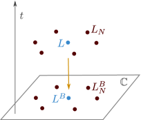
Figure 2: Single-wrapped and multiwrapped lines, both in the bulk ($t>0$) and on the boundary ($t=0$) of $[0,\infty)\times M_{q}$, in the case $N=6$. We have illustrated the fiber above a single point $[x]\in S^{1}$.

As we have emphasized, ${\mathcal{L}}_{\mathfrak{q}}$ is not an algebra, so we cannot literally say that ${\mathcal{L}}_{\pm}$ is “central” in ${\mathcal{L}}_{\mathfrak{q}}$. Nevertheless, the multiwrapping map ${\mathcal{L}}_{\pm}\to{\mathcal{L}}_{\mathfrak{q}}$ plays a role on the boundary analogous to the role the multiwrapping map ${\mathcal{A}}_{\pm}\to{\mathcal{A}}_{\mathfrak{q}}$ plays in the bulk. Furthermore, we can combine a multi-wrapped boundary line with a standard boundary line at the origin to give an action ${\mathcal{L}}_{\pm}\times{\mathcal{L}}_{\mathfrak{q}}\to{\mathcal{L}}_{\mathfrak{q}}$, promoting ${\mathcal{L}}_{\mathfrak{q}}$ to a module for ${\mathcal{L}}_{\pm}$.

In particular, we can use this map to study the structure of ${\mathcal{L}}_{\mathfrak{q}}$. Using the bulk multiwrapping map we have an action of ${\mathcal{A}}_{\pm}$ on ${\mathcal{L}}_{\mathfrak{q}}$, and the quotients ${\mathcal{L}}_{\mathfrak{q}}/I_{x}{\mathcal{L}}_{\mathfrak{q}}$ for $x\in{\mathcal{M}}_{\pm}[T]$ are still supported on the Lagrangian subspace ${\mathcal{M}}_{\pm}[B]$. They are modules for the corresponding quotients ${\mathcal{A}}_{\mathfrak{q}}/I_{x}{\mathcal{A}}_{\mathfrak{q}}$. Finally, if ${\mathcal{L}}_{\pm}$ is not generated by ${\mathcal{A}}_{\pm}$ acting on the identity, we can further decompose these modules under the action of the commutative algebra ${\mathcal{L}}_{\pm}$, to get smaller sheaves over the spectrum of ${\mathcal{L}}_{\pm}$.

2.7 An orbifold defect in 3d

In this section we briefly discuss another point of view on our construction. Assume that $q$ is a primitive $N^{\mathrm{th}}$ root of unity. We can dimensionally reduce along the fibration

$$\pi_{2}:M_{q}\to\mathbb{C}/\mathbb{Z}_{N}$$ (32)

defined by $\pi_{2}:[(z,x)]\mapsto[z]$. The reduced theory is thus a 3d theory on a supersymmetric orbifold ${\mathbb{C}}/\mathbb{Z}_{N}\times{{\mathbb{R}}}$. We can think of this as the 3d theory in the presence of a codimension-2 supersymmetric defect, supported at the orbifold line. Passing to an appropriate topological twist of the 3d theory, the orbifold should be invisible and we should be able to treat this as a standard line defect.

We can then move to the 3d Coulomb branch, where the 3d theory has an effective description as an IR-free non-linear sigma-model with target ${\mathcal{M}}_{\pm}[T]$. In this setup a supersymmetric codimension-2 defect should admit an effective description in terms of some auxiliary finite-dimensional quantum-mechanical system coupled to the sigma model, i.e. a hyperholomorphic sheaf $V_{\mathfrak{q}}$ on ${\mathcal{M}}_{\pm}[T]$ which is a finite-rank vector bundle at least over a Zariski open subset of ${\mathcal{M}}_{\pm}[T]$ Thompson:2000pw . Considering UV line defects at $z=0$ as local operators on the orbifold defect would give a map from ${\mathcal{A}}_{\mathfrak{q}}$ to the space of global sections of ${\mathrm{End}}(V_{\mathfrak{q}})$, compatible with the identification of the multiwrapped subalgebra ${\mathcal{A}}_{\pm}\subset{\mathcal{A}}_{\mathfrak{q}}$ with functions on ${\mathcal{M}}_{\pm}[T]$.

We will now assume that this map is actually an isomorphism. This is a non-trivial assumption: it means that operators which are different in the UV will act differently on the IR data, and every possible operator in the IR description is the image of some UV operator. We will not try to justify this assumption. It is analogous to the observation that ${\mathcal{A}}_{\pm}$ is exactly the algebra of holomorphic functions on ${\mathcal{M}}_{\pm}$, rather than just mapping into it; that appears to be true in practice, but we are not aware of a proof of it.

At any rate, under this assumption, we could glean information about ${\mathcal{A}}_{\mathfrak{q}}$ by considering the sheaf of quotient algebras ${\mathcal{A}}_{\mathfrak{q}}/I_{x}{\mathcal{A}}_{\mathfrak{q}}$ over ${\mathcal{M}}_{\pm}[T]$, where $I_{x}\subset{\mathcal{A}}_{\pm}$ are the maximal ideals associated to points $x\in{\mathcal{M}}_{\pm}[T]$: for sufficiently general $x$, these quotients should generically be finite-dimensional matrix algebras, the fibers of ${\mathrm{End}}(V_{\mathfrak{q}})$.

In various concrete cases, the statement that the fibers ${\mathcal{A}}_{\mathfrak{q}}/I_{x}{\mathcal{A}}_{\mathfrak{q}}$ are matrix algebras for sufficiently general $x\in{\mathcal{M}}_{\pm}$ is known in the mathematics literature — see e.g. Bonahon_2015 ; Bonahon_2017 ; bonahon2015representations ; karuo2022azumaya for skein algebras, MR1124981 ; BECK199429 for quantized universal enveloping algebras, and Fock:2003xxy for cluster varieties. One would like to understand more precisely what “sufficiently general $x$” should mean; for the $\operatorname{{\mathfrak{sl}}}(2)$ skein algebras this question is answered precisely in karuo2022azumaya , and it would be interesting to understand the answer in physical terms.

One new statement we are making here is that the sheaf of algebras ${\mathcal{A}}_{\mathfrak{q}}$ and the sheaf of representations $V_{\mathfrak{q}}$ carry natural hyperholomorphic structures over the hyperkähler space ${\mathcal{M}}_{\pm}[T]$. One could go further and attempt to construct these hyperholomorphic structures concretely. This can be done explicitly in the simple case where $T$ is a pure abelian ${\mathcal{N}}=2$ gauge theory. More generally, one should be able to start with the IR abelian gauge theory and improve it by corrections coming from BPS particles to give the desired hyperholomorphic connections; this would involve an extension of the TBA-type integral equation methods of Gaiotto:2008cd ; hhlb ; Gaiotto:2011tf . It would be very interesting to develop this extension in detail.

3 Examples

3.1 Pure $U(1)$ gauge theory

Let us consider the simplest example, the pure 4d ${\mathcal{N}}=2$ gauge theory with gauge group $U(1)$. In this theory there are Wilson-’t Hooft line defects ${\mathfrak{L}}_{\gamma}$ labeled by electromagnetic charge $\gamma=(e,m)\in{{\mathbb{Z}}}^{2}$,with Dirac-Schwinger-Zwanziger pairing ${\langle{\gamma,\gamma^{\prime}}\rangle}=em^{\prime}-me^{\prime}$.

We denote the single-wrapped Wilson line with unit positive charge as $L_{1,0}\equiv X$, and the single-wrapped ’t Hooft line with unit positive charge as $L_{0,1}\equiv P$. For generic $q\neq 1$, we have the relation in ${\mathcal{A}}_{\mathfrak{q}}$

$$XP=qPX\,,$$ (33)

defining the quantum torus algebra. More generally,

$$L_{e,m}L_{e^{\prime},m^{\prime}}={\mathfrak{q}}^{em^{\prime}-me^{\prime}}L_{e+e^{\prime},m+m^{\prime}}\,.$$ (34)

Notice that the algebras ${\mathcal{A}}_{\mathfrak{q}}$ and ${\mathcal{A}}_{-{\mathfrak{q}}}$ can be identified by the transformation $L_{e,m}\to(-1)^{em}L_{e,m}$. The identification is not canonical: it depends on a choice of electric-magnetic duality frame. When $q$ is a primitive $N$-th root of unity, the quantum torus has a large center, which is precisely spanned by the $L_{\gamma,N}=L_{N\gamma}$, as expected. As discussed in the previous section, the algebra of the $L_{N\gamma}$ can be canonically identified with the commutative algebra ${\mathcal{A}}_{{\mathfrak{q}}^{N^{2}}}$.

We can localize the algebra ${\mathcal{A}}_{\mathfrak{q}}$ by setting $X^{N}=x$, $P^{N}=p$ for some $x,p\in{\mathbb{C}}^{\times}$. The quotient of ${\mathcal{A}}_{\mathfrak{q}}$ by these relations is an algebra of dimension $N^{2}$. Moreover, for any given $(x,p)$ we can represent $X$ and $P$ by clock and shift operators; this identifies the quotient as the algebra of $N\times N$ complex matrices, in keeping with our discussion in subsection 2.7.

Next, we can introduce some half-BPS boundary conditions.

3.1.1 The pure Dirichlet / Neumann boundary condition

The simplest examples are the Dirichlet and pure Neumann boundary conditions. As they are related by electric-magnetic duality, we only really need to describe one of them.

At a Dirichlet boundary, the $U(1)$ gauge symmetry becomes a global symmetry. As we compactify this boundary condition on the circle, we get a family of Dirichlet boundary conditions $D_{\mu}$, labeled by the background holonomy $\mu\in{\mathbb{C}}^{\times}$.

The Wilson line brought to the boundary becomes a flavour Wilson line, and thus acting on the boundary we have $X=\mu$. The left ideal generated by $X-\mu$ determines the left ${\mathcal{A}}_{\mathfrak{q}}$-module ${\mathcal{L}}_{\mathfrak{q}}[D_{\mu}]={\mathcal{A}}_{\mathfrak{q}}/{\mathcal{A}}_{\mathfrak{q}}(X-\mu)$. This module is free on the basis $\{P^{r}:r\in{{\mathbb{Z}}}\}$.

Now suppose $q$ is a primitive $N$-th root of unity. On the boundary we have the relation $X_{N}=\mu^{N}$, so the commutative algebra ${\mathcal{L}}_{\pm}[D_{\mu}]\subset{\mathcal{L}}_{\mathfrak{q}}[D_{\mu}]$ of multiwrapped operators on the boundary is freely generated by $P_{N}=P^{N}$ alone.

We can localize the algebra ${\mathcal{A}}_{\mathfrak{q}}$ by setting $X^{N}=x$, $P^{N}=p$. We find that the ${\mathcal{A}}_{\mathfrak{q}}$-module ${\mathcal{L}}_{\mathfrak{q}}[D_{\mu}]$ is supported on the Lagrangian $x=\mu^{N}$, as expected. The localized module is $N$-dimensional and gives the above-mentioned clock-and-shift representation for the localized algebra.

So far we discussed pure Dirichlet boundary conditions. In the case of pure Neumann boundary conditions all the same discussion applies, with the roles of $X$ and $P$ exchanged.

3.1.2 Neumann boundary conditions enriched by a chiral multiplet

We can also consider a simple type of enriched Neumann boundary condition: a 3d ${\mathcal{N}}=2$ chiral multiplet coupled to the restriction of the bulk $U(1)$ gauge field. Let $a\in{{\mathbb{Z}}}$ be the charge of this boundary chiral multiplet.

For $a=1$, line defects brought to the boundary obey the tetrahedron relation (see Dimofte:2011ju equation (7.5)):

$$X+P=1.$$ (35)

The module ${\mathcal{L}}_{\mathfrak{q}}$ is the quotient of ${\mathcal{A}}_{\mathfrak{q}}$ by the left ideal generated by this relation.

When $q$ is a primitive $N$-th root of unity, our discussion predicts that the multiwrapped lines $X_{N}$ and $P_{N}$ should obey the relation defining ${\mathcal{L}}_{\pm}$, which is again (35). We can check this directly:

$$\begin{split}P_{N}&=P^{N}=(1-X)P^{N-1}\\ &=P^{N-1}(1-q^{N-1}X)\\ &=P^{N-2}(1-q^{N-2}X)(1-q^{N-1}X)\\ &=(1-X)\cdots(1-q^{N-2}X)(1-q^{N-1}X)\\ &=1+(-1)^{N}q^{\frac{N(N-1)}{2}}X^{N}=1-X_{N}~{}~{}\text{for}~{}~{}q=\text{e}^{2\pi\text{i}/N}\end{split}$$ (36)

as desired.

The case of general $a$ follows easily from the $a=1$ case by redefining the charge lattice. Starting from

$$P^{a}=P^{a-1}(1-X)=(1-q^{a-1}X)P^{a-1}=\cdots=(1-X)(1-qX)\cdots(1-q^{a-1}X)$$ (37)

and replacing $P^{a}\to P$, $X\to X^{a}$ (which follows from the relation between the charge lattice of the charge $a$ chiral multiplet and the theory with $a=1$) we obtain the correct generalization of (35):

$$P=(1-X^{a})(1-qX^{a})\cdots(1-q^{a-1}X^{a})\,.$$ (38)

Similarly, taking the $a^{\mathrm{th}}$ power of the charge-$1$ relation

$$P_{N}^{a}=(1-X_{N})^{a}\,,$$ (39)

and substituting $P_{N}^{a}\to P_{N}$, $X_{N}\to X_{N}^{a}$, we obtain the desired relation

$$P_{N}=(1-X_{N}^{a})^{a}\,.$$ (40)

(Note that a direct verification starting from (38) is slightly involved.)

3.2 The $U(1)$ theory with one hypermultiplet

Now let us briefly discuss the 4d ${\mathcal{N}}=2$ theory with gauge group $U(1)$ coupled to a hypermultiplet with charge $1$. In this case the algebra ${\mathcal{A}}_{\mathfrak{q}}$ is slightly more interesting; it is generated by lines $X$, $Y$, $Z^{\pm 1}$ with relations

$$XY =1+{\mathfrak{q}}^{-1}Z,$$ (41)

$$YX =1+{\mathfrak{q}}Z,$$ (42)

$$YZ ={\mathfrak{q}}^{2}ZY,$$ (43)

$$XZ ={\mathfrak{q}}^{-2}ZX.$$ (44)

Here $X$ and $Y$ are ’t Hooft loops with magnetic charge $+1$ and $-1$ respectively, and $Z^{n}$ is the Wilson loop with electric charge $n$. These equations can be deduced from the wall-crossing formulae in Gaiotto:2010be and the bulk BPS spectrum of the theory. In particular, each of $X$, $Y$, $Z^{\pm 1}$ has a chamber in which it supports only one framed BPS state. We can rewrite (41) as wall-crossing equations on the overlap of chambers. But these overlaps are Zariski open, so the relations hold universally. It follows that the multiwrapping map is $X_{N}=X^{N}$, $Y_{N}=Y^{N}$, $Z_{N}^{\pm 1}=Z^{\pm N}$.

When $q$ is a primitive $N$-th root of unity, we can check directly that $X^{N}$, $Y^{N}$, $Z^{\pm N}$ are central. Moreover, we check

$$X^{N}Y^{N}=X^{N-1}(1+{\mathfrak{q}}^{-1}Z)Y^{N-1} =(1+{\mathfrak{q}}Z)X^{N-1}Y^{N-1}$$ (45)

$$=(1+{\mathfrak{q}}Z)(1+{\mathfrak{q}}^{3}Z)X^{N-2}Y^{N-2}$$ (46)

$$=(1+{\mathfrak{q}}Z)(1+{\mathfrak{q}}^{3}Z)\cdots(1+{\mathfrak{q}}^{2N-1}Z)$$ (47)

$$=1\pm Z^{N}$$ (48)

with the sign $\pm 1={\mathfrak{q}}^{N^{2}}$ as usual. This confirms that the generators $X^{N}$, $Y^{N}$, $Z^{N}$ obey the classical relations in ${\mathcal{A}}_{\pm 1}$, i.e. the multiwrapping map embeds ${\mathcal{A}}_{\pm 1}\to{\mathcal{A}}_{\mathfrak{q}}$, as we expect.

We can also give a geometric representation of the line operators in this theory, using its class ${\mathcal{S}}$ realization as the compactification of the 6d $(2,0)$ theory of type $\operatorname{{\mathfrak{sl}}}(2)$ on a sphere with a single irregular singularity. There are four Stokes directions and four anti-Stokes directions associated with this irregular singularity. We illustrate this in subsection 3.2, where we cut out an infinitesimal disc around the irregular singularity. Each Stokes direction carries a labeling by an ordered pair of integers, which keep track of the sheets of a double cover of the boundary circle. The ’t Hooft lines $X$ and $Y$ correspond to open paths connecting two anti-Stokes directions which are not adjacent to each other; each end of the open paths carries a label, specifying one of the sheets of the double cover. Finally, the Wilson lines $Z^{\pm 1}$ are represented by loops traveling around the boundary of the cut-out disc, also carrying a sheet label.

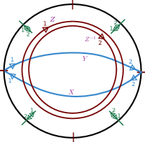
Figure 3: Here we show $\mathbb{CP}^{1}$ minus an infinitesimal disc around an irregular singularity placed at infinity. There are four Stokes directions at the boundary of the disc labeled by green markers, as well as four anti-Stokes directions labeled by red markers. The numbered arrows indicate the canonical orientations on the double cover of $\mathbb{CP}^{1}$ minus the disc. The ’t Hooft lines $X$ and $Y$ (in blue) correspond to open paths connecting two non-adjacent anti-Stokes directions, while the Wilson lines $Z^{\pm}$ (in red) correspond to loops around the boundary of the disc.

The relations obeyed by the line operators now follow from $\operatorname{{\mathfrak{sl}}}(2)$ skein relations on the disc. Rather than formulating and checking these skein relations directly, it is convenient to use the UV-IR map to an abelian skein algebra associated with a branched double cover of the disc; we can compute this map using the methods of Neitzke:2020jik . For example, the verification of (41) is illustrated in subsection 3.2.

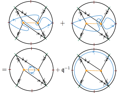
Figure 4: Here we illustrate the two lifts of $XY$ in the abelian skein algebra, with their simplification using the abelian skein relations.

3.3 Class ${\mathcal{S}}$ theories on the four-punctured sphere

Next we discuss some more elaborate ${\mathcal{N}}=2$ theories. We will use class ${\mathcal{S}}$ descriptions of the theories as a convenient tool for computation Klemm:1996bj ; Witten:1997sc ; Gaiotto:2009we ; Gaiotto:2009hg .

We begin with the $SU(2)$ theory with $N_{f}=4$, realized as a class ${\mathcal{S}}$ theory of type $A_{1}$ on the sphere with four regular punctures. In this theory, BPS line defects correspond to isotopy classes of simple closed curve on the four-punctured sphere Drukker:2009id ; Gaiotto:2010be . We consider the two line defects $L^{A,B}$ shown in Figure 5.

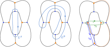
Figure 5: Left, center: two $1/2$-BPS UV line defects in the $SU(2)$ $N_{f}=4$ theory, represented as loops on the four-punctured sphere. Right: the IR electromagnetic charges $\gamma_{1}$, $\gamma_{2}$, represented as cycles on the Seiberg-Witten curve. The blue dots indicate the four punctures; orange crosses indicate the branch points of the Seiberg-Witten curve (49); black arcs show the spectral network associated to the Seiberg-Witten curve.

We will study their IR expansions at a point in the strong coupling region, where the framed BPS spectrum is especially simple. The corresponding Seiberg-Witten curve is

$$\widetilde{C}=\{\lambda:\lambda^{2}+\phi_{2}=0\}\subset T^{*}C,\quad\phi_{2}=-\frac{z^{4}+2z^{2}-1}{2(z^{4}-1)^{2}}dz^{2}.$$ (49)

We express the electromagnetic charges relative to a basis $\{\gamma_{1},\gamma_{2}\}$ with $\langle\gamma_{1},\gamma_{2}\rangle=-1$, also shown in the figure. To shorten expressions we will suppress flavour charges, keeping only the electromagnetic charge.

The Wilson line $L^{A}$ has the following IR expansion Neitzke:2020jik :

$$L^{A}=X_{(1,0)}+X_{(-1,0)}+X_{(-1,2)}+2X_{(0,1)}+2X_{(-1,1)}.$$ (50)

Given this expression we can directly compute the Chebyshev polynomial $T_{N}(L^{A})$ at $q=\text{e}^{2\pi\text{i}/N}$. Using Mathematica, we verified for $N\leq 5$ that it does have the expected expression, obtained by replacing each $\gamma\to N\gamma$:

$$T_{N}(L^{A})=X_{(N,0)}+X_{(-N,0)}+X_{(-N,2N)}+2X_{(0,N)}+2X_{(-N,N)}.$$ (51)

The line defect $L^{B}$ has a more complicated IR expansion, which can be obtained e.g. using the methods of Neitzke:2020jik ; Bonahon_2015 :

$$\begin{split}L^{B}=&\ X_{(-1,1)}+2X_{(-1,2)}+X_{(-1,3)}+6X_{(0,1)}+2({\mathfrak{q}}+{\mathfrak{q}}^{-1})X_{(0,2)}+X_{(1,-1)}\\ &+6X_{(1,0)}+(4+{\mathfrak{q}}^{2}+{\mathfrak{q}}^{-2})X_{(1,1)}+2X_{(2,-1)}+2({\mathfrak{q}}+{\mathfrak{q}}^{-1})X_{(2,0)}+X_{(3,-1)}.\end{split}$$ (52)

Again we verified that $T_{N}(L^{B})$ at $q=\text{e}^{2\pi\text{i}/N}$ looks as expected (for $N=2,3$): we replace each $\gamma\to N\gamma$ and also replace ${\mathfrak{q}}\to{\mathfrak{q}}^{N^{2}}=\pm 1$,

$$\begin{split}T_{N}(L^{B})=&\ X_{(-N,N)}+2X_{(-N,2N)}+X_{(-N,3N)}+6X_{(0,N)}\pm 4X_{(0,2N)}+X_{(N,-N)}\\ &+6X_{(N,0)}+6X_{(N,N)}+2X_{(2N,-N)}\pm 4X_{(2N,0)}+X_{(3N,-N)}\end{split}$$ (53)

All this matches with the expectations from the previous sections, and with the theorems of bonahon2015representations . We remark that this provides a nice check on the IR expansions of line defects; if one modifies the expansion (52), say by changing one of the coefficients, then this match typically does not work out anymore.

Now let us move on to the case of an $A_{2}$ theory of class ${\mathcal{S}}$, again on the four-punctured sphere, with all four punctures “full” in the sense of Gaiotto:2009we . This theory is an $SU(3)$ gauging of two copies of the Minahan-Nemeschansky $E_{6}$ theory Gaiotto:2009we .

The expectations in the $A_{2}$ case are slightly more complicated than for $A_{1}$. If $L$ is a fundamental Wilson line in a weak coupling region, and $\overline{L}$ the corresponding antifundamental Wilson line, then instead of (30) we will have IR expansions of the form

$$L=X+Y+(XY)^{-1}\,,\quad\overline{L}=X^{-1}+Y^{-1}+XY\,,$$ (54)

where $X$ and $Y$ commute. Similarly

$$L_{N}=X^{N}+Y^{N}+(XY)^{-N},\quad\overline{L}_{N}=X^{-N}+Y^{-N}+(XY)^{N}\,.$$ (55)

Using these expansions we can write $L_{N}$ as a polynomial in $L$ and $\overline{L}$, the higher-rank generalization of the Chebyshev polynomials which appeared in the $A_{1}$ case. For instance,

$$L_{2}=L^{2}-2\overline{L}\,,\qquad L_{3}=L^{3}-3L\overline{L}+3\,.$$ (56)

As before, although we used a weak-coupling region to derive these relations, it follows that they hold at any point of the Coulomb branch.

At some points of the Coulomb branch, we can verify (56) directly using the methods of Neitzke:2021gxr . Namely, consider a point of the Coulomb branch where the Seiberg-Witten curve is

$$\widetilde{C}=\{\lambda:\lambda^{3}+\phi_{2}\lambda+\phi_{3}=0\}\subset T^{*}C,$$ (57)

where $\phi_{3}$ is very small and $\phi_{2}$ is as in (49) above. In this case the IR expansions of the line defects are quite long; even for $L^{A}$ we already have $48$ terms $X_{\gamma}$, with each $\gamma$ a vector of length $8$ (since in this theory the electromagnetic charge lattice has rank $8$). Still, with computer assistance we verified that the IR expansions of $L^{A}$ and $\overline{L^{A}}$ indeed obey the expected relations when $q$ is a primitive $N$-th root of unity, for $N=2$ or $N=3$. For instance, evaluating $L^{A}_{2}=(L^{A})^{2}-2\overline{L^{A}}$ for $q=-1$, one obtains again 48 terms, and these 48 terms match what one obtains by starting with the IR expansion of $L^{A}$, setting ${\mathfrak{q}}=1$, and replacing $X_{\gamma}\to X_{2\gamma}$ in each term.

The arXiv version of this paper includes an ancillary Mathematica file which performs these verifications (including the flavour charges, and also including a slight additional enhancement to treat the theories of type $\operatorname{{\mathfrak{gl}}}(2)$ and $\operatorname{{\mathfrak{gl}}}(3)$ rather than $A_{1}$ and $A_{2}$.)

3.4 Coulomb branch algebras and quantum groups

In this section we discuss several classes of quantized Coulomb branch algebras which are related to quantum groups, and the corresponding root-of-unity phenomena.

3.4.1 Quantum groups and class ${\mathcal{S}}$

First we consider theories of class ${\mathcal{S}}$ Klemm:1996bj ; Witten:1997sc ; Gaiotto:2009we ; Gaiotto:2009hg . Recall that these theories are obtained by twisted compactification of 6d $(2,0)$ theories, labelled by an ADE Lie algebra ${\mathfrak{g}}$, on a Riemann surface $C$ possibly decorated with punctures and/or twist lines. The 3d Coulomb branch of a class ${\mathcal{S}}$ theory is a character variety, i.e. a moduli space of flat ${\mathfrak{g}}$-connections on $C$.

The relation to quantum groups arises when we consider class ${\mathcal{S}}$ theories in the case of a surface $C$ with a rank 1 irregular puncture (and any number of other punctures, regular or irregular). By a “rank $1$ irregular puncture” we mean a puncture where the flat ${\mathfrak{g}}$-connection has a second-order pole with semisimple residue. The Stokes data at such a puncture consists of matrices $S^{\pm}$ in opposite Borel subgroups of $G$, together with a formal monodromy matrix $W$ in the Cartan subgroup $H$. The total monodromy around the puncture is $S^{+}WS^{-}$.

To be precise, the theories we need to consider are not exactly the usual class ${\mathcal{S}}$ theories. In a class ${\mathcal{S}}$ theory with a rank $1$ irregular puncture, there is a global $H$ symmetry; the formal monodromy $W$ is fixed in terms of mass parameters for that symmetry, and the matrix elements of $S^{\pm}$ are not well-defined functions on the 3d Coulomb branch: rather, they are well defined only up to the conjugation action of $H$. We modify the class ${\mathcal{S}}$ theory by gauging this global $H$ symmetry. This enlarges the 3d Coulomb branch: it makes $W$ into a function on the Coulomb branch rather than a fixed mass parameter, and removes the identification under conjugation by $H$. The matrix elements of $S^{\pm}$, along with $W$, are well defined functions on the enlarged 3d Coulomb branch; thus they give elements of ${\mathcal{A}}_{1}$.

The matrices $S^{\pm}$ and $W$ associated with a rank $1$ irregular puncture have another interpretation: they parameterize the “dual Poisson-Lie group” $G^{*}$, as originally observed in boalchpoissonlie . Thus we have a map $\mu:{\mathcal{O}}(G^{*})\to{\mathcal{A}}_{1}$. Moreover, this map is actually a Poisson map, and it is known that it lifts to a map between the standard quantizations on the two sides: on the one hand ${\mathcal{A}}_{1}$ quantizes to ${\mathcal{A}}_{\mathfrak{q}}$ as we have been discussing, on the other hand ${\mathcal{O}}(G^{*})$ can be quantized to give the quantum group $U_{q}({\mathfrak{g}})$, and there is a canonical algebra map $U_{q}({\mathfrak{g}})\to{\mathcal{A}}_{\mathfrak{q}}$ Gaiotto:2014lma ; alex2019quantum ; schradershapiro ; shenqg .

If we take ${\mathfrak{q}}$ to be a primitive root of unity with ${\mathfrak{q}}^{N^{2}}=1$, then our general setup predicts that there must be a canonical multiwrapping map ${\mathcal{A}}_{1}\to{\mathcal{A}}_{\mathfrak{q}}$, whose image is central. Anticipating a result from the next section, this multiwrapping map is in an appropriate sense local on $C$. As a consequence, we can focus just on the neighborhood of the irregular singularity. Thus we predict that the composite map ${\mathcal{O}}(G^{*})\to{\mathcal{A}}_{1}\to{\mathcal{A}}_{\mathfrak{q}}$ should factor through a map ${\mathcal{O}}(G^{*})\to U_{q}({\mathfrak{g}})$, in a manner independent of the geometry of the rest of $C$. When ${\mathfrak{q}}^{N^{2}}=-1$ we have a similar statement, replacing $G^{*}$ by its ${\mathfrak{q}}=-1$ analog which we call $G^{*}_{-}$.

In other words, our setup predicts that when $q$ is a primitive root of unity, the center of $U_{q}({\mathfrak{g}})$ should contain a copy of ${\mathcal{O}}(G^{*})$ or ${\mathcal{O}}(G_{-}^{*})$. This is indeed a well known fact in the theory of quantum groups, as described e.g. in MR1124981 ; BECK199429 .

Finally we remark that the map $U_{q}({\mathfrak{g}})\to{\mathcal{A}}_{\mathfrak{q}}$ is compatible with the coproduct and R-matrix of $U_{q}({\mathfrak{g}})$, relating them to the amalgamation of character varieties in the sense of MR2263192 ; alex2019quantum ; shenqg . The amalgamation procedure can be given a physical interpretation, as governing the behaviour of the class ${\mathcal{S}}$ theories in a limit where the gauge coupling associated to the irregular singularity becomes very large. It should be possible to use this interpretation to define 3d ${\cal N}=2$ interfaces which implement the amalgamation/coproduct, and thus physically derive the observation that when $q$ is a root of unity the coproduct localizes on its classical limit, i.e. the Poisson map $G^{*}\times G^{*}\to G^{*}$ which makes $G^{*}$ into a Poisson-Lie group.

3.4.2 Quantum groups and linear quivers

Another physical setting where quantum groups appear is that of 4d linear quiver gauge theories with $n-1$ nodes and unitary gauge groups. In these theories, the 3d Coulomb branch can be described as a moduli space of solutions to the Bogomolny equations for $SL(n)$ on $\mathbb{R}\times\mathbb{C}^{*}$, in the presence of Dirac singularities. On general grounds, one can define an infinite collection of holomorphic functions on such a space (not linearly independent), organized as elements of a “scattering matrix” $T(z)$, a $n\times n$ matrix of Laurent polynomials. Remarkably, this structure survives quantization Bullimore:2015lsa ; Frassek:2020lky , in the form of an algebra map from the loop quantum group $U_{q}(L\mathfrak{sl}(n))$ to the quantized Coulomb branch ${\mathcal{A}}_{\mathfrak{q}}$.

This map can be given a physical interpretation via dualities starting from Witten’s geometric engineering construction Witten:1997sc . Witten’s construction presents the 4d theory as sitting on a collection of D4 branes, coupled to a collection of NS5 branes. The worldvolume theory of the NS5 branes decouples in the 4d field theory limit. Nevertheless, the 4d theory must admit a supersymmetric coupling to the 6d worldvolume theory. Upon compactification on $M_{q}$, we expect the 6d theory to reduce to 4d holomorphic-topological Chern-Simons theory with coupling $(2\pi{\mathrm{i}})^{-1}\log q$ compactified on $\mathbb{C}^{*}$ Costello:2021zcl , while the 4d theory reduces to a quantum-mechanical system coupled to the HT Chern-Simons theory as a topological line defect.. This conjecture is a trigonometric version of the constructions in Ishtiaque:2018str ; Costello:2021zcl ; Dedushenko:2020yzd . The coupling can be precisely expressed via Koszul duality as an algebra map from an “universal gauge algebra” $U_{q}(L\mathfrak{sl}(n))$ for the 4d CS theory to the algebra of local operators of the quantum-mechanical system, i.e. ${\mathcal{A}}_{\mathfrak{q}}$.

The role of $M_{q}$ in this discussion strongly suggests that the root-of-unity behavior we have discussed should also apply to $U_{q}(L{\mathfrak{g}})$ itself, i.e. $U_{q}(L{\mathfrak{g}})$ should have a center isomorphic to the space of functions of scattering matrices $T(z)$ (or its ${\mathfrak{q}}=-1$ analog). This should be compatible with the root-of-unity phenomena in the individual 4d gauge theories. As $U_{q}(L{\mathfrak{g}})$ and its scattering matrices play an important role in integrability, it would be nice to explore the potential applications of the root-of-unity construction in that context, e.g. for the Chiral Potts Model.

3.4.3 Combining these constructions

In the last two subsections we discussed two different ways of relating quantum groups to quantized Coulomb branches: either using class ${\mathcal{S}}$ theories or linear quivers. There are some examples which can be obtained in both ways. In these cases the expected map $U_{q}(L{\mathfrak{g}})\to{\mathcal{A}}_{\mathfrak{q}}$ associated to the brane realization factors through the well-known map $U_{q}(L{\mathfrak{g}})\to U_{q}({\mathfrak{g}})$ to give the map $U_{q}({\mathfrak{g}})\to{\mathcal{A}}_{\mathfrak{q}}$ arising from the class ${\mathcal{S}}$ construction.

The simplest example is a linear quiver with gauge groups $U(1)\times\cdots\times U(n-1)$ and $n$ flavours at the last node. This quiver theory admits a class ${\mathcal{S}}$ realization with ${\mathfrak{g}}=\operatorname{{\mathfrak{sl}}}(N)$, associated to a sphere with a rank $1$ irregular singularity and a regular singularity, following a general recipe given in Witten:1997sc ; Gaiotto:2009hg .

In this case the character variety is parameterized by $S^{\pm}$ and $W$ with the constraint that $S^{+}WS^{-}$ belongs to a fixed conjugacy class, determined by the mass parameter for the flavour symmetry associated to the regular singularity. Thus the Coulomb branch is the intersection of $G^{*}$ and a regular orbit of ${\mathfrak{g}}$. This Coulomb branch is quantized to a central quotient of $U_{q}({\mathfrak{g}})$.

Again, it should be possible to push our analysis to derive statements about the coproduct on $U_{q}({\mathfrak{g}})$ when $q$ is a root of unity.

3.4.4 A simple example

We continue with the setup of the last subsection, further specialized to the case $n=2$ (${\mathfrak{g}}=\operatorname{{\mathfrak{sl}}}_{2}$). In this case the quiver theory is $U(1)$ gauge theory coupled to $2$ hypermultiplets of charges $\pm 1$, with a $SU(2)$ flavour symmetry acting on the hypermultiplets. Thus this case is particularly simple since it only involves an abelian gauge group; in contrast, for $n\geq 3$ we would have a nonabelian gauge theory. A description of this example from the point of view of quantized cluster algebra is given in Example 4.7 of schradershapiro and in Section 15.6 of alex2019quantum ; here we describe it from the point of view of the algebras of line operators.

Let $Z^{\pm 1}$ denote the Wilson lines with electric charges $\pm 1$, and let $X$, $Y$ be ’t Hooft lines with magnetic charges $+1$ and $-1$ respectively. Let $\mu$ denote the $SU(2)$ flavour mass. In the quantized theory these line defects obey

$$XY =(1+{\mathfrak{q}}^{-1}\mu Z)(1+{\mathfrak{q}}\mu Z^{-1})\,,$$ (58)

$$YX =(1+{\mathfrak{q}}\mu Z)(1+{\mathfrak{q}}^{-1}\mu Z^{-1})\,,$$ (59)

$$YZ ={\mathfrak{q}}^{2}ZY\,,$$ (60)

$$XZ ={\mathfrak{q}}^{-2}ZX\,.$$ (61)

These relations are similar to those we discussed in subsection 3.2, and can similarly be derived from wall-crossing. When $q^{N}=1$, the multiwrapping map ${\mathcal{A}}_{\pm}\to{\mathcal{A}}_{\mathfrak{q}}$ is given by $X_{N}=X^{N}$, $Y_{N}=Y^{N}$, $Z^{\pm 1}_{N}=Z^{\pm N}$, just as in subsection 3.2.

The relations (58)-(61) imply in particular

$$XY-YX =({\mathfrak{q}}^{-1}-{\mathfrak{q}})\mu(Z-Z^{-1})\,,$$ (62)

$$XY+YX -({\mathfrak{q}}^{-1}+{\mathfrak{q}})\mu(Z+Z^{-1})=2+2\mu^{2}\,.$$ (63)

Then if we introduce

$$E =\frac{X}{{\mathfrak{q}}^{-1}-{\mathfrak{q}}}\,,$$ (64)

$$F =\mu^{-1}\frac{Y}{{\mathfrak{q}}^{-1}-{\mathfrak{q}}}\,,$$ (65)

$$K =Z\,,$$ (66)

we see that $E$, $F$, $K$ satisfy the standard defining relations of $U_{q}(\operatorname{{\mathfrak{sl}}}_{2})$, with the quadratic Casimir $\frac{1}{2}(({\mathfrak{q}}^{-1}-{\mathfrak{q}})^{2}(EF+FE)-({\mathfrak{q}}^{-1}+{\mathfrak{q}})(K+K^{-1}))$ fixed to $\mu+\mu^{-1}$.

Setting ${\mathfrak{q}}=-1$ in the relations (58)-(61) we see that ${\mathcal{A}}_{-}$ is a commutative algebra on generators $X$, $Y$, $Z^{\pm 1}$, $\mu^{\pm 1}$ with the relation $\mu^{-1}XY=\mu+\mu^{-1}-(Z+Z^{-1})$. This algebra is naturally identified with ${\mathcal{O}}(G^{*}_{-})\simeq{\mathcal{O}}(G^{*})$. Indeed, $Z^{\pm 1}$ become the eigenvalues of the formal monodromy $W$; $X$ and $\mu^{-1}Y$ become the off-diagonal entries of the Stokes matrices $S^{+}W^{1/2}$ and $W^{1/2}S^{-}$; $\mu^{\pm 1}$ become the eigenvalues of the actual monodromy $S^{+}WS^{-}$. This version of the $q\to 1$ limit, giving a commutative algebra, is the one that arises naturally in our 4-dimensional setup.

In contrast, the more conventional description of the $q\to 1$ limit of $U_{q}({\mathfrak{g}})$ leads to the noncommutative algebra $U({\mathfrak{g}})$. That limit corresponds to reducing our 4-dimensional setup to a 3-dimensional theory in $\Omega$-background, by writing $q={\mathrm{e}}^{2\pi{\mathrm{i}}R\hbar}$ and taking $R\to 0$ at fixed $\hbar$, as we discussed in subsection 2.4.

We can also give an explicit geometric representation for the Wilson and ’t Hooft lines in this theory, using its class ${\mathcal{S}}$ description as the compactification of the 6d $(2,0)$ theory of type $\operatorname{{\mathfrak{sl}}}(2)$ on a sphere with a regular singularity and a rank-$1$ irregular singularity. This is illustrated in subsubsection 3.4.4, where we cut out an infinitesimal disc around the irregular singularity and draw its complement in the sphere. There are two Stokes directions and two anti-Stokes directions associated with the irregular singularity. The Wilson lines $Z^{\pm 1}$ with electric charges $\pm 1$ are represented by loops traveling near the boundary of the disc. The ’t Hooft lines $X$, $Y$ with magnetic charges $\pm 1$ correspond to open paths beginning and ending at the anti-Stokes directions. As in subsection 3.2 these paths carry some additional sheet labels. We note that the flavor charges of the ’t Hooft lines realized here are slightly different from those of (58)-(61): the blue open paths in subsubsection 3.4.4 correspond to lines $X^{\prime},Y^{\prime}$ with

$$X^{\prime}=X,~{}Y^{\prime}=\mu^{-1}Y.$$ (67)

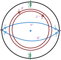
Figure 6: Here we illustrate $\mathbb{CP}^{1}$ minus an infinitesimal disc around an irregular singularity placed at infinity. There are two Stokes directions at the boundary of the disc, represented by green markers, and two anti-Stokes directions represented by red markers. The ’t Hooft lines $X^{\prime}$ and $Y^{\prime}$ (in blue) correspond to open paths ending on the red markers at the boundary. The Wilson lines $Z$ and $Z^{-1}$ correspond to loops traveling around the boundary.

From the geometrical point of view, the relations (58)-(61) obeyed by line defects follow from $\operatorname{{\mathfrak{sl}}}(2)$ skein relations on the punctured disc. As we did in subsection 3.2 we check these relations by lifting to the abelian skein algebra associated with a branched double cover of the disc, following the prescriptions of Neitzke:2020jik . For example, subsubsection 3.4.4 illustrates four lifts of $X^{\prime}Y^{\prime}$ into the abelian skein algebra, which yields

$$X^{\prime}Y^{\prime}=\mu+\mu^{-1}+{\mathfrak{q}}^{-1}Z+{\mathfrak{q}}Z^{-1}.$$ (68)

This recovers (58) up to the convention (67).

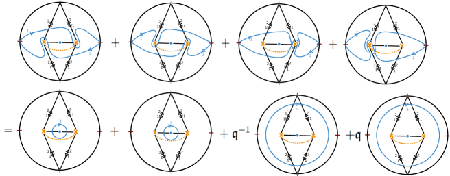
Figure 7: Here we illustrate the four lifts of $X^{\prime}Y^{\prime}$ in the abelian skein algebra, together with their simplification using the abelian skein relations.

4 Class ${\mathcal{S}}$ theories and the Kapustin-Witten twist

There is an alternative point of view on the root-of-unity phenomena in class ${\mathcal{S}}$ theories, which emerges from a connection to the Kapustin-Witten twist of $N=4$ super Yang-Mills.

4.1 The large center from Kapustin-Witten twist

Fix a surface $C$ and Lie algebra ${\mathfrak{g}}$. As in the previous section, we will ignore topological subtleties associated to the global form of the group. The ${\mathfrak{g}}$-character variety of $C$ coincides with the phase space of 3d Chern-Simons theory compactified on $C$. The natural classical observables on this phase space are (networks of) Wilson lines, or “skeins,” in $M=C\times\mathbb{R}$. When ${\mathfrak{g}}$ is a complex Lie algebra their algebra reproduces the algebra of holomorphic functions on the character variety.

The Chern-Simons path integral provides a natural quantization of this classical phase space. The standard path-integration contour is only well-defined if the Chern-Simons level $\kappa$ is appropriately quantized. More generally, the path integral can be done in an “analytically continued” manner for any level $\kappa\in{\mathbb{C}}$ Witten:2010cx ; Witten:2010zr . This theory provides a canonical quantization of the algebra of observables, i.e. a quantization of the algebra of holomorphic functions on the character variety; this is the skein algebra $\mathrm{Sk}_{\mathfrak{q}}[{\mathfrak{g}},C]$ with parameter ${\mathfrak{q}}=\exp\frac{{\mathrm{i}}\pi}{\kappa}$.

The analytically continued Chern-Simons path integral on a 3-manifold $M$ can be given a more robust definition, as the path integral for the Kapustin-Witten twist Kapustin:2006pk of 4d ${\mathcal{N}}=4$ super Yang-Mills with parameter $\Psi=\kappa$, on $M\times[0,\infty)_{t}$, with Neumann boundary conditions at $t=0$. Thus the Chern-Simons theory is “relative” and cannot be assigned a canonical Hilbert space.

From this point of view, the skein algebra is realized by skeins of boundary Wilson line defects, and the root-of-unity phenomena arise from a special property of the Kapustin-Witten twist, as follows. For a generic value of $\Psi$, the twisted theory does not admit any line defects. When $\Psi=p/q\in{\mathbb{Q}}$, the situation is different: a ’t Hooft-Wilson line labeled by electric and magnetic weights $(\lambda,\lambda^{\vee})$ survives into the twisted theory exactly if $q\lambda=p\lambda^{\vee}$ Kapustin:2006pk . Thus for $\Psi\in{\mathbb{Q}}$ (equivalently, for ${\mathfrak{q}}$ a root of unity) the twisted theory has a family of bulk line defects labeled by weights; they are pure Wilson lines in the special case $\Psi=\infty$, and pure ’t Hooft lines if $\Psi=0$. When bulk lines do exist, we can make skeins out of them, and then bring them to the Neumann boundary; the resulting boundary skeins are central in the skein algebra $\operatorname{Sk}_{\mathfrak{q}}[{\mathfrak{g}},C]$, since they are free to move in the fourth dimension. Thus we obtain a large center in $\operatorname{Sk}_{\mathfrak{q}}[{\mathfrak{g}},C]$, isomorphic to the algebra of functions on the character variety.

4.2 A duality

We have now given two different physical points of view on the appearance of the large center in $\operatorname{Sk}_{\mathfrak{q}}[{\mathfrak{g}},C]$: one in section 2 using an ${\mathcal{N}}=2$ theory of class ${\mathcal{S}}$, the other in subsection 4.1 using ${\mathcal{N}}=4$ super Yang-Mills.

The two pictures are related by a chain of dualities. Indeed, we simply need to consider the 6d $(2,0)$ theory of type ${\mathfrak{g}}$ on $M_{q}\times C\times{{\mathbb{R}}}$, with a twist along $C$. We can view this setup in two ways:

• Reducing first on the $C$ factor gives a class ${\mathcal{S}}$ theory on $M_{q}\times{{\mathbb{R}}}$. This is the setup we used in section 2.

• If we replace the $z$-plane in $M_{q}$ by a cigar and reduce along its circle direction, the 6d theory reduces to 5d super Yang-Mills theory on a half-space. The boundary corresponds to the locus $z=0$ in $M_{q}$, and carries a principal Nahm pole boundary condition from the 5d perspective. Reducing along the $x$-circle in $M_{q}$ corresponds to a further circle reduction of the 5d super Yang-Mills, with a twist by the instanton charge; the resulting system is 4d ${\mathcal{N}}=4$ SYM on $[0,\infty)\times C\times{{\mathbb{R}}}$, with coupling $\Psi=\frac{1}{\pi{\mathrm{i}}}\log{\mathfrak{q}}$ and a principal Nahm pole boundary condition. Finally, S-duality maps this to coupling $\Psi^{-1}=\frac{1}{\pi{\mathrm{i}}}\log{\mathfrak{q}}$ and a Neumann boundary condition. This is the setup we discussed in subsection 4.1.

This sketchy derivation can be made more precise by twisting. The 6d $(2,0)$ theory admits a holomorphic-topological twist with four topological directions. We can repeat the above reduction using the twisted theory on $M_{q}\times C\times{{\mathbb{R}}}$, where the holomorphic direction is the $z$-plane in $M_{q}$. The twisted theory then reduces to the holomorphic-topological twist of the class ${\mathcal{S}}$ theory on $M_{q}\times{{\mathbb{R}}}$, and to the Kapustin-Witten twist of ${\mathcal{N}}=4$ super Yang-Mills on $[0,\infty)\times C\times{{\mathbb{R}}}$.

Now let us revisit the skeins of Chern-Simons theory in $C\times{{\mathbb{R}}}$. From the 6-dimensional perspective, we can realize these skeins as 2-dimensional defects: they are the product of a skein in $C\times{{\mathbb{R}}}$ and the geodesic $\psi_{0}$ in $M_{q}$. (Note that these defects continue to exist in the 6-dimensional holomorphic-topological twist, since they are extended only in the 4 topological directions.) In the class ${\mathcal{S}}$ theory, these defects reduce to supersymmetric line defects in $M_{q}\times{{\mathbb{R}}}$ wrapping $\psi_{0}$ in $M_{q}$. In ${\mathcal{N}}=4$ SYM, they become boundary Wilson line skeins lying on the Neumann boundary condition.

When $q$ is a root of unity, we can also consider “multiwrapping” these 2-dimensional defects, by putting them on the product of a skein in $C\times{{\mathbb{R}}}$ and one of the geodesics $\psi_{z_{0}}$ in $M_{q}$. These multiwrapped defects reduce to the multiwrapped line defects in the class ${\mathcal{S}}$ theory, and to the bulk skeins in the ${\mathcal{N}}=4$ SYM theory. Thus the two ways we obtained the large center in $\operatorname{Sk}_{\mathfrak{q}}[{\mathfrak{g}},C]$ are indeed related by our 6-dimensional setup.

We conclude with a few remarks:

1. The 4d SYM perspective allows one further manipulation. We can find an element of the $SL(2,{{\mathbb{Z}}})$ duality group (generalized $S$-duality) which maps $\Psi=m/N$ to $\Psi=\infty$, where the bulk lines are Wilson lines. Correspondingly, this duality maps the Nahm boundary condition to a more general “$(N,m)$-fivebrane” boundary condition.

   We can attempt to describe this $(N,m)$-fivebrane boundary condition as the result of coupling the 4d gauge theory to a 3d SCFT ${\cal T}_{N,m}[{\mathfrak{g}}]$. To do so, we consider the 4d theory on an interval, where at one end we place the $(N,m)$ boundary condition, and at the other end we place a Dirichlet boundary condition; the resulting 3d theory should be ${\cal T}_{N,m}[{\mathfrak{g}}]$. The Dirichlet boundary condition fixes the value of the bulk skeins, so effectively the algebra of skeins in ${\cal T}_{N,m}[{\mathfrak{g}}]$ is a quotient of the full skein algebra, where the central elements are fixed to specific values determined by a point of the character variety. In this way one should be able to identify the theories ${\cal T}_{N,m}[{\mathfrak{g}}]$ with the ones considered in Creutzig:2021ext .

2. A direct consequence of the 4d SYM description is that the construction of $L_{N}$ from $L$ must be a local operation on the skein representing $L$: a bulk line labelled by a representation $R$ must correspond to a boundary line in some (possibly virtual) representation $R_{N}$. We have already seen examples of this, for skeins consisting of a single loop. Similarly, the intertwiners at the junctions of bulk lines must map universally to intertwiners of boundary lines, not depending on the rest of the skein.

   In other words, the construction of $L_{N}$ should follow from a categorical statement about the braided category of lines in analytically continued Chern-Simons theory and the center which appears at roots of unity.

3. Class ${\mathcal{S}}$ theories come equipped with a large collection of “class $R$” boundary conditions, arising from the compactification of the $(2,0)$ 6d theories on 3d manifolds $D$ with cylindrical asymptotic regions Dimofte:2013lba .

   In the 3d Coulomb branch perspective, such a boundary condition is supported on the Lagrangian submanifold of flat connections on $C$ which extend to $D$. Boundary line defects arise from skeins in $D$; upon quantization they give rise to skein modules. For some background on the notion of skein module see e.g. MR1194712 ; 2023arXiv230214734J .

   Following the general picture in subsection 2.6, we predict some additional structure when $q$ is a root of unity. First, the skein module associated to a class $R$ boundary condition will be supported on its classical image in the character variety. Second, this skein module will admit a large submodule which has a natural commutative algebra structure. Concretely, this algebra structure arises from the fact that the skeins in the image of the multiwrapping map can be freely isotoped across one another, so there is a well defined operation of juxtaposing them.

Acknowledgements

We thank Pablo Boixeda Alvarez, Francis Bonahon, Daniel Douglas, Alexander Goncharov, David Jordan, and Ivan Losev for useful discussions. This research was supported in part by a grant from the Krembil Foundation. D.G. is supported by the NSERC Discovery Grant program and by the Perimeter Institute for Theoretical Physics. Research at Perimeter Institute is supported in part by the Government of Canada through the Department of Innovation, Science and Economic Development Canada and by the Province of Ontario through the Ministry of Colleges and Universities. A.N. is supported by NSF grant DMS-2005312. G.M. and F.Y. is supported by DOE grant DE-SC0010008.

References

- (1) H. G. Groenewald, “On the principles of elementary quantum mechanics,” Physica 12 (1946) 405–460.
- (2) L. V. Hove, “Sur les problèmes des relations entre les transformations unitaires de la mécanique quantique et les transformations canoniques de la mécanique classique,” Acad. Roy. Belgique Bull. Cl. Sci 37 (1951) 610–20.
- (3) I. Todorov, “Quantization is a mystery,” 1206.3116.
- (4) M. Kontsevich, “Deformation quantization of Poisson manifolds. 1.,” Lett. Math. Phys. 66 (2003) 157–216, q-alg/9709040.
- (5) A. Kapustin and D. Orlov, “Remarks on A branes, mirror symmetry, and the Fukaya category,” J. Geom. Phys. 48 (2003) 84, hep-th/0109098.
- (6) A. Kapustin, “A-branes and noncommutative geometry,” hep-th/0502212.
- (7) S. Gukov and E. Witten, “Branes and Quantization,” Adv. Theor. Math. Phys. 13 (2009), no. 5, 1445–1518, 0809.0305.
- (8) N. A. Nekrasov and S. L. Shatashvili, “Quantization of Integrable Systems and Four Dimensional Gauge Theories,” in 16th International Congress on Mathematical Physics, pp. 265–289. 8, 2009. 0908.4052.
- (9) N. Nekrasov and E. Witten, “The Omega Deformation, Branes, Integrability, and Liouville Theory,” JHEP 09 (2010) 092, 1002.0888.
- (10) E. Witten, “A New Look At The Path Integral Of Quantum Mechanics,” 1009.6032.
- (11) J. Yagi, “-deformation and quantization,” JHEP 08 (2014) 112, 1405.6714.
- (12) M. Bullimore, T. Dimofte, and D. Gaiotto, “The Coulomb Branch of 3d Theories,” Commun. Math. Phys. 354 (2017), no. 2, 671–751, 1503.04817.
- (13) C. Beem, W. Peelaers, and L. Rastelli, “Deformation quantization and superconformal symmetry in three dimensions,” Commun. Math. Phys. 354 (2017), no. 1, 345–392, 1601.05378.
- (14) V. Pestun, “Localization of gauge theory on a four-sphere and supersymmetric Wilson loops,” Commun. Math. Phys. 313 (2012) 71–129, 0712.2824.
- (15) L. F. Alday, D. Gaiotto, S. Gukov, Y. Tachikawa, and H. Verlinde, “Loop and surface operators in N=2 gauge theory and Liouville modular geometry,” JHEP 01 (2010) 113, 0909.0945.
- (16) N. Drukker, J. Gomis, T. Okuda, and J. Teschner, “Gauge Theory Loop Operators and Liouville Theory,” JHEP 02 (2010) 057, 0909.1105.
- (17) D. Gaiotto, G. W. Moore, and A. Neitzke, “Framed BPS States,” Adv. Theor. Math. Phys. 17 (2013), no. 2, 241–397, 1006.0146.
- (18) T. Dimofte, D. Gaiotto, and S. Gukov, “3-Manifolds and 3d Indices,” Adv. Theor. Math. Phys. 17 (2013), no. 5, 975–1076, 1112.5179.
- (19) V. V. Fock and A. B. Goncharov, “Cluster ensembles, quantization and the dilogarithm,” math/0311245.
- (20) S. Cecotti, A. Neitzke, and C. Vafa, “R-Twisting and 4d/2d Correspondences,” 1006.3435.
- (21) F. Bonahon and H. Wong, “Representations of the Kauffman bracket skein algebra I: invariants and miraculous cancellations,” Inventiones mathematicae 204 (Jul, 2015) 195–243, 1206.1638v3.
- (22) F. Bonahon and H. Wong, “Representations of the Kauffman bracket skein algebra, II: Punctured surfaces,” Algebraic and Geometric Topology 17 (Oct, 2017) 3399–3434, 1206.1639v3.
- (23) J. Korinman and A. Quesney, “Classical shadows of stated skein representations at roots of unity,” 1905.03441.
- (24) C. Frohman and J. Kania-Bartoszynska, “The structure of the Kauffman bracket skein algebra at roots of unity,” Math. Z. 289 (2018), no. 3-4, 889–920.
- (25) C. De Concini and V. G. Kac, “Representations of quantum groups at roots of ,” in Operator algebras, unitary representations, enveloping algebras, and invariant theory (Paris, 1989), vol. 92 of Progr. Math., pp. 471–506. Birkhäuser Boston, Boston, MA, 1990.
- (26) C. De Concini, V. G. Kac, and C. Procesi, “Quantum coadjoint action,” J. Amer. Math. Soc. 5 (1992), no. 1, 151–189.
- (27) J. Beck, “Representations of quantum groups at even roots of unity,” Journal of Algebra 167 (1994), no. 1, 29–56.
- (28) M. A. Melvin, “Pure magnetic and electric geons,” Phys. Lett. 8 (1964) 65–70.
- (29) N. Nekrasov and A. Okounkov, “Seiberg-Witten theory and random partitions,” Prog. Math. 244 (2006) 525–596, hep-th/0306238.
- (30) S. Hellerman, D. Orlando, and S. Reffert, “The Omega Deformation From String and M-Theory,” JHEP 07 (2012) 061, 1204.4192.
- (31) A. Braverman, M. Finkelberg, and H. Nakajima, “Towards a mathematical definition of Coulomb branches of -dimensional gauge theories, II,” Adv. Theor. Math. Phys. 22 (2018) 1071–1147, 1601.03586.
- (32) A. Kapustin and E. Witten, “Electric-Magnetic Duality And The Geometric Langlands Program,” Commun. Num. Theor. Phys. 1 (2007) 1–236, hep-th/0604151.
- (33) D. Gaiotto and E. Witten, “Janus Configurations, Chern-Simons Couplings, And The theta-Angle in N=4 Super Yang-Mills Theory,” JHEP 06 (2010) 097, 0804.2907.
- (34) D. Gaiotto and E. Witten, “S-Duality of Boundary Conditions In N=4 Super Yang-Mills Theory,” Adv. Theor. Math. Phys. 13 (2009), no. 3, 721–896, 0807.3720.
- (35) D. Gaiotto and E. Witten, “Supersymmetric Boundary Conditions in N=4 Super Yang-Mills Theory,” J. Statist. Phys. 135 (2009) 789–855, 0804.2902.
- (36) E. Witten, “Analytic Continuation Of Chern-Simons Theory,” AMS/IP Stud. Adv. Math. 50 (2011) 347–446, 1001.2933.
- (37) E. Witten, “Fivebranes and Knots,” Quantum Topol. 3 (2012) 1–137, 1101.3216.
- (38) D. Gaiotto and E. Witten, “Knot Invariants from Four-Dimensional Gauge Theory,” Adv. Theor. Math. Phys. 16 (2012), no. 3, 935–1086, 1106.4789.
- (39) T. Dimofte, M. Gabella, and A. B. Goncharov, “K-Decompositions and 3d Gauge Theories,” JHEP 11 (2016) 151, 1301.0192.
- (40) C. Beem, T. Dimofte, and S. Pasquetti, “Holomorphic Blocks in Three Dimensions,” JHEP 12 (2014) 177, 1211.1986.
- (41) T. Dimofte, D. Gaiotto, and R. van der Veen, “RG Domain Walls and Hybrid Triangulations,” Adv. Theor. Math. Phys. 19 (2015) 137–276, 1304.6721.
- (42) A. Braverman, M. Finkelberg, and H. Nakajima, “Coulomb branches of quiver gauge theories and slices in the affine Grassmannian,” Adv. Theor. Math. Phys. 23 (2019) 75–166, 1604.03625.
- (43) R. Bezrukavnikov and D. Kaledin, “Fedosov quantization in positive characteristic,” arXiv Mathematics e-prints (Jan., 2005) math/0501247, math/0501247.
- (44) B. Webster, “Coherent sheaves and quantum Coulomb branches I: tilting bundles from integrable systems,” arXiv e-prints (May, 2019) arXiv:1905.04623, 1905.04623.
- (45) M. Aganagic, K. Costello, J. McNamara, and C. Vafa, “Topological Chern-Simons/Matter Theories,” 1706.09977.
- (46) K. Costello, T. Dimofte, and D. Gaiotto, “Boundary Chiral Algebras and Holomorphic Twists,” 2005.00083.
- (47) S. Cautis and H. Williams, “Cluster theory of the coherent Satake category,” arXiv e-prints (Jan., 2018) arXiv:1801.08111, 1801.08111.
- (48) G. W. Moore, N. Nekrasov, and S. Shatashvili, “Integrating over Higgs branches,” Commun. Math. Phys. 209 (2000) 97–121, hep-th/9712241.
- (49) G. W. Moore, N. Nekrasov, and S. Shatashvili, “D particle bound states and generalized instantons,” Commun. Math. Phys. 209 (2000) 77–95, hep-th/9803265.
- (50) N. A. Nekrasov, “Seiberg-Witten prepotential from instanton counting,” Adv. Theor. Math. Phys. 7 (2003), no. 5, 831–864, hep-th/0206161.
- (51) C. Beem, D. Ben-Zvi, M. Bullimore, T. Dimofte, and A. Neitzke, “Secondary products in supersymmetric field theory,” Annales Henri Poincare 21 (2020), no. 4, 1235–1310, 1809.00009.
- (52) D. Gaiotto, G. W. Moore, and E. Witten, “Algebra of the Infrared: String Field Theoretic Structures in Massive Field Theory In Two Dimensions,” 1506.04087.
- (53) M. Kontsevich and Y. Soibelman, “Stability structures, motivic Donaldson-Thomas invariants and cluster transformations,” 0811.2435.
- (54) L. Hollands and A. Neitzke, “Spectral Networks and Fenchel–Nielsen Coordinates,” Lett. Math. Phys. 106 (2016), no. 6, 811–877, 1312.2979.
- (55) G. Thompson, “Holomorphic vector bundles, knots and the Rozansky-Witten invariants,” Adv. Theor. Math. Phys. 5 (2002) 457–481, hep-th/0002168.
- (56) F. Bonahon and H. Wong, “Representations of the Kauffman bracket skein algebra III: closed surfaces and naturality,” 1505.01522.
- (57) H. Karuo and J. Korinman, “Azumaya loci of skein algebras,” 2211.13700.
- (58) D. Gaiotto, G. W. Moore, and A. Neitzke, “Four-dimensional wall-crossing via three-dimensional field theory,” Commun. Math. Phys. 299 (2010) 163–224, 0807.4723.
- (59) A. Neitzke, “On a hyperholomorphic line bundle over the Coulomb branch,” 1110.1619.
- (60) D. Gaiotto, G. W. Moore, and A. Neitzke, “Wall-Crossing in Coupled 2d-4d Systems,” JHEP 12 (2012) 082, 1103.2598.
- (61) S. Alexandrov and B. Pioline, “Theta series, wall-crossing and quantum dilogarithm identities,” Lett. Math. Phys. 106 (2016), no. 8, 1037–1066, 1511.02892.
- (62) V. Fock and A. Goncharov, “Geometric quantization of cluster varieties.” To appear.
- (63) T. Dimofte, D. Gaiotto, and S. Gukov, “Gauge Theories Labelled by Three-Manifolds,” Commun. Math. Phys. 325 (2014) 367–419, 1108.4389.
- (64) F. Costantino and T. T. Q. Lê, “Stated skein algebras of surfaces,” J. Eur. Math. Soc. (JEMS) 24 (2022), no. 12, 4063–4142.
- (65) A. Neitzke and F. Yan, “-nonabelianization for line defects,” JHEP 09 (2020) 153, 2002.08382.
- (66) T. T. Q. Lê and T. Yu, “Quantum traces and embeddings of stated skein algebras into quantum tori,” Selecta Math. (N.S.) 28 (2022), no. 4, Paper No. 66, 48.
- (67) A. Klemm, W. Lerche, P. Mayr, C. Vafa, and N. P. Warner, “Self-Dual Strings and N=2 Supersymmetric Field Theory,” Nucl. Phys. B477 (1996) 746–766, hep-th/9604034.
- (68) E. Witten, “Solutions of four-dimensional field theories via M theory,” Nucl. Phys. B 500 (1997) 3–42, hep-th/9703166.
- (69) D. Gaiotto, “N=2 dualities,” JHEP 08 (2012) 034, 0904.2715.
- (70) D. Gaiotto, G. W. Moore, and A. Neitzke, “Wall-crossing, Hitchin systems, and the WKB approximation,” Adv. Math. 234 (2013) 239–403, 0907.3987.
- (71) A. Neitzke and F. Yan, “The quantum UV-IR map for line defects in (3)-type class S theories,” JHEP 09 (2022) 081, 2112.03775.
- (72) P. P. Boalch, “Stokes matrices, Poisson Lie groups and Frobenius manifolds,” Invent. Math. 146 (2001), no. 3, 479–506.
- (73) D. Gaiotto, “Open Verlinde line operators,” 1404.0332.
- (74) A. Goncharov and L. Shen, “Quantum geometry of moduli spaces of local systems and representation theory,” 1904.10491.
- (75) G. Schrader and A. Shapiro, “A cluster realization of from quantum character varieties,” Invent. Math. 216 (2019), no. 3, 799–846, 1607.00271.
- (76) L. Shen, “Cluster nature of quantum groups,” 2209.06258.
- (77) V. V. Fock and A. B. Goncharov, “Cluster -varieties, amalgamation, and Poisson-Lie groups,” in Algebraic geometry and number theory, vol. 253 of Progr. Math., pp. 27–68. Birkhäuser Boston, Boston, MA, 2006.
- (78) R. Frassek, V. Pestun, and A. Tsymbaliuk, “Lax matrices from antidominantly shifted Yangians and quantum affine algebras: A-type,” Adv. Math. 401 (2022) 108283, 2001.04929.
- (79) K. Costello, D. Gaiotto, and J. Yagi, “Q-operators are ’t Hooft lines,” 2103.01835.
- (80) N. Ishtiaque, S. Faroogh Moosavian, and Y. Zhou, “Topological holography: The example of the D2-D4 brane system,” SciPost Phys. 9 (2020), no. 2, 017, 1809.00372.
- (81) M. Dedushenko and D. Gaiotto, “Correlators on the wall and sln spin chain,” J. Math. Phys. 63 (2022), no. 9, 092301, 2009.11198.
- (82) T. Creutzig, T. Dimofte, N. Garner, and N. Geer, “A QFT for non-semisimple TQFT,” 2112.01559.
- (83) J. H. Przytycki, “Skein modules of -manifolds,” Bull. Polish Acad. Sci. Math. 39 (1991), no. 1-2, 91–100.
- (84) D. Jordan, “Langlands duality for skein modules of 3-manifolds,” arXiv e-prints (Feb., 2023) arXiv:2302.14734, 2302.14734.