Environmental effects on associations of dwarf galaxies

Abstract

We study the properties of associations of dwarf galaxies and their dependence on the environment. Associations of dwarf galaxies are extended systems composed exclusively of dwarf galaxies, considering as dwarf galaxies those galaxies less massive than $M_{\star,\rm max}=10^{9.0}$ ${\rm M}_{\odot}\,h^{-1}$. We identify these particular systems using a semi-analytical model of galaxy formation coupled to a dark matter only simulation in the $\Lambda$ Cold Dark Matter cosmological model. To classify the environment, we estimate eigenvalues from the tidal field of the dark matter particle distribution of the simulation. We find that the majority, two thirds, of associations are located in filaments ($\sim 67$ per cent), followed by walls ($\sim 26$ per cent), while only a small fraction of them are in knots ($\sim 6$ per cent) and voids ($\sim 1$ per cent). Associations located in more dense environments present significantly higher velocity dispersion than those located in less dense environments, evidencing that the environment plays a fundamental role in their dynamical properties. However, this connection between velocity dispersion and the environment depends exclusively on whether the systems are gravitational bound or unbound, given that it disappears when we consider associations of dwarf galaxies that are gravitationally bound. Although less than a dozen observationally detected associations of dwarf galaxies are currently known, our results are predictions on the eve of forthcoming large surveys of galaxies, which will enable these very particular systems to be identified and studied.

1 Introduction

The large-scale structure map of the Universe reveals that galaxy and dark matter distributions are not uniform, describing an intricate interconnected network known as the cosmic web. Within this network, galaxies, intergalactic gas, and dark matter are distributed within high density regions as groups and clusters of galaxies, or along filaments and sheet-like walls, which surround very low density regions known as voids. Most of the galaxies embedded in this cosmic web belong to systems which can contain from a few to hundreds even thousands of members (Huchra & Geller, 1982; Yang et al., 2007; Tempel et al., 2012). These systems have been extensively studied and there is ample evidence that many of their observed properties are influenced by the web-like environment (Dressler, 1980; Kauffmann et al., 2004; O’Mill et al., 2008; Peng et al., 2010; Zheng et al., 2017; Duplancic et al., 2020, among others). For example, it is known that elliptical galaxies are located more frequently in denser regions, while spiral galaxies are more common in the field (Dressler, 1980). Similar trends are also detected for colours, star formation history and the ages of galaxies (Blanton et al., 2005); in denser environments, there is a higher proportion of red and passive galaxies for a given stellar mass (Wetzel et al., 2012; Wang et al., 2018). On the other hand, from a theoretical point of view, many studies show that the orientation of the haloes’ minor axes shows a tendency to be perpendicular to the wall or filament where they reside. The spin orientation also correlates with the halo mass, being parallel to the filaments or walls for low-mass haloes and perpendicular for higher mass haloes (Aragón-Calvo et al., 2007; Hahn et al., 2007a, b; Zhang et al., 2009; Libeskind et al., 2013, among others).

Groups of galaxies are a particular type of system, being the most common structures of galaxies in the Universe. Even though there is no clear demarcation between groups and clusters, the latest one are generally considered to contain hundreds or thousands of galaxies while groups contain only a few, with $\sim 50$ being the most commonly used cut-off value when defining them. Their typical sizes are on average compared to a spherical volume of $\sim 1\,{\rm Mpc}$ of diameter. Their virial masses are, on average, approximately $\sim 10^{13}\,{\rm M}_{\odot}\,h^{-1}$ and the velocity dispersion of their galaxy members are about $\sim 150\,{\rm km\,s^{-1}}$. These groups can host very bright galaxies as well as fainter galaxies. However, the pioneering work of Tully (1987) revealed the existence of a very striking type of groups called ‘associations of dwarf galaxies’. These systems have the particularity of being extended systems , with typical sizes of $\sim 0.2\,{\rm Mpc}\,h^{-1}$, composed only of dwarf galaxies, extracted from the Nearby Galaxies Catalog (Tully, 1988). They use a merging-tree algorithm to define these systems, where the luminosity density, determined by the combined luminosities and separations of contributing systems, was used to characterize the linkages between galaxies. Two levels of structure, namely ‘groups’ and ‘associations’ were defined based on luminosity density thresholds. We focus on ‘associations of dwarf galaxies’ derived from linkages between galaxies that had insignificant luminosities, making the luminosity density fail to reach the threshold required to be classified as a group (see Tully 1987 for a exhaustive depiction of the method).

Among the very few works that study these particular systems, Tully et al. (2006) present a detailed description of the only seven associations of dwarf galaxies observed up to now and their main dynamical properties. Among these properties we can highlight their velocity dispersions covering a range between $\sim 20$ and $\sim 75\,{\rm km\,s^{-1}}$, their sizes around $0.2\,{\rm Mpc}\,h^{-1}$ and their virial masses ranging between $\sim 10^{10.5}$ and $\sim 10^{11.8}\,{\rm M}_{\odot}\,h^{-1}$. From the theoretical point of view, Yaryura et al. (2020) present a study of associations of dwarf galaxies in the cosmological framework of the $\Lambda$ Cold Dark Matter ($\Lambda$CDM) model, applying a semi-analytic model of galaxy formation to a dark matter-only N-body numerical simulation. They conclude that the $\Lambda$CDM model is able to reproduce these particular systems. On average, these simulated systems have typical sizes of $\sim 0.2\,{\rm Mpc}\,h^{-1}$, velocity dispersions of $\sim 30\,{\rm km\,s^{-1}}$ and estimated total masses of $\sim 10^{11}\,{\rm M}_{\odot}\,h^{-1}$. These main dynamical properties mean values are comparable to the observational results presented by Tully et al. (2006). In comparison with groups of galaxies, these associations present lower masses and velocity dispersions despite their large size. Their low masses, in addition to their low luminosity, suggest that their mass–to–light ratio is relatively high if these systems are bound systems. Based on this assertion, Tully et al. (2006) infer that these associations are bound but dynamically unevolved systems. They also suggest that they presumably contain dark matter subhaloes ranging from $10^{9}$ to $10^{10}$ $M_{\odot}$ which contain insufficient amounts of gas and stars to be detected at present.

So far only a few of these associations have been observed and very little is known about their properties. But these systems are of fundamental importance because they could be used as a probe of the cosmological model, if a substantial number of them will be detected in future surveys. Currently, the standard paradigm, $\Lambda$CDM, is a theory predicting evolution of haloes due to mergers. In fact, at virtually any given moment in cosmic time, dark matter haloes undergo mergers. The relevant time scales here are well known. Therefore, it is intriguing to examine the nature of associations that withstand the cosmic forces of tides and gravity.

From the observational point of view, although currently only less than a dozen of these systems of dwarf galaxies are known, their study holds significant importance in anticipation of upcoming galaxy surveys, such as the Dark Energy Spectroscopic Instrument (DESI), the Vera C. Rubin Observatory (Ivezić et al. 2019), the 4-metre Multi-Object Spectroscopic Telescope (4MOST, de Jong et al. 2019), among many others. These surveys hold the promise of providing a highly detailed map of the Local Universe, facilitating the detection of faint galaxies that have remained elusive until now. By detecting these faint galaxies, we anticipate the possibility of identifying new systems exclusively composed of dwarf galaxies. In this sense, our findings will consist of theoretical predictions that await observational confirmation when these future galaxy catalogs become available.

The main goal of this paper is to deepen the theoretical understanding of these associations of dwarf galaxies by analysing the large-scale environment within which they form and evolve, and to study how their main dynamical properties vary with the environment. For this, we use the semi-analytic model of galaxy formation sag (acronym for Semi-Analytic Galaxies, Cora et al., 2018) coupled to the $400\,h^{-1}\,{\rm Mpc}$ Small MultiDark Planck simulation (smdpl) based on the Planck cosmology (Klypin et al., 2016). smdpl simulation is publicly available in the CosmoSim database .

This paper is organized as follows. We describe the smdpl simulation and the sag model in Section 2. In Section 3, we define our sample of associations of dwarf galaxies and describe their main properties. Section 4 classifies the large-scale environment and analyses the dependence of the properties of the associations on the environment. In Section 5, we summarize our main results and present our conclusions.

Parameter	Best-fitting value
$\alpha$	0.08
$\epsilon$	0.53
$\epsilon_{\rm ejec}$	0.01
$f_{\rm BH}$	0.07
$\kappa_{\rm AGN}$	1.18 $\times$ 10-5
$f_{\rm pert}$	31.22
$\gamma$	0.005
$f_{\rm hot,sat}$	0.26

Table 1: Best-fitting values of the free parameters of sag model obtained with the PSO technique. This set of values is obtained from the application of sag to the merger trees of the subbox selected from the SMDPL simulation.

2 Hybrid model of galaxy formation

The sample of associations of dwarf galaxies is extracted from a galaxy catalogue constructed by applying a hybrid model of galaxy formation that couples a semi-analytical model of galaxy formation and evolution with a dark matter-only cosmological simulation. Below, we briefly describe the main aspects of this model.

2.1 Dark matter cosmological simulation

We use the smdpl dark matter-only cosmological simulation, which follows the evolution of $3840^{3}$ particles from redshift $z=120$ to $z=0$, within a (relatively) small volume (a periodic box of side-length of $400\,{\rm Mpc}\,h^{-1}$). This large number of particles within such a volume reaches a mass resolution of $9.63\times 10^{7}\,{\rm M}_{\odot}\,h^{-1}$ per dark matter (DM) particle (see Klypin et al. 2016 for more details). smdpl cosmological parameters are given by a flat $\Lambda$CDM model consistent with Planck measurements: $\Omega_{\rm m}$ = 0.307, $\Omega_{\rm B}$ = 0.048, $\Omega_{\Lambda}$ = 0.693, $\sigma_{8}$ = 0.829, $n_{\rm s}$ = 0.96 and $h$ = 0.678, (Planck Collaboration et al., 2014).

The Rockstar halo finder (Behroozi et al., 2013a) is used to identify DM haloes keeping just overdensities with at least $N_{\text{min}}$ = 20 DM particles. There are two classifications of DM haloes: main host haloes (detected over the background density) and subhaloes (that lie inside other DM haloes). From these haloes, ConsistentTrees (Behroozi et al., 2013b) constructs merger trees, by linking haloes and subhaloes forwards and backwards in time to progenitors and descendants, respectively.

2.2 Semi-analytic model of galaxy formation SAG

In this project, we follow Yaryura et al. (2020) and use the latest version of the semi-analytic model sag presented in Cora et al. (2018), based on the model previously presented by Springel et al. (2001). This is an updated and improved version, including the main physical processes required for galaxy formation: gas cooling, star formation in quiescent and bursty modes (being the latter triggered by disc instabilities and mergers), black hole growth, feedback from supernovae and active galactic nuclei (AGN), environmental effects (ram pressure stripping and tidal stripping), chemical enrichment. The circulation of mass and metals among the different baryonic components (hot gas halo, cold gas disc, stellar disc and bulge) are regulated by ejection and reincorporation mechanisms associated to feedback processes and recycling of stellar mass. We refer the reader to Cora et al. (2018) for a detailed and exhaustive description of the model.

Each sag galaxy populates a DM halo of the simulation in such a way that central galaxies correspond to main host haloes while satellite galaxies are hosted by subhaloes, according to the information provided by the merger trees. A satellite galaxy is defined as an orphan galaxy when its DM substructure is no longer detected by the halo finder. The position and velocity of orphan galaxies are obtained following the model introduced by Delfino et al. (2022) to calculate the orbital evolution of unresolved subhaloes.

The main galaxy properties provided by sag are listed in Knebe et al. (2018, see their Table A2), although the information of many other properties can be obtained as requested by a given project. The properties used in the current work are: a pointer to the DM halo in which a galaxy orbits; galaxy type (central galaxy, satellite with DM substructure, orphan satellite); positions and velocities of a galaxy; stellar mass of a galaxy, $M_{\star}$; mass of the main host DM halo in which a galaxy resides, $M_{200}$. The halo mass is defined as the mass enclosed by a sphere of radius $r_{200}$, within which the mean density is a factor $\Delta=200$ times the critical density of the Universe $\rho_{\textrm{c}}$, i.e.,

$$M_{\textrm{200}}(<r_{\textrm{200}})=\Delta\rho_{\textrm{c}}\frac{4\pi}{3}r_{\textrm{200}}^{3}.$$ (1)

To regulate the physical processes involved in the sag model, a set of free parameters are employed: the star formation efficiency ($\alpha$); the efficiency of SN feedback from stars formed in both the disc and the bulge ($\epsilon$); the efficiency of ejection of gas from the hot phase ($\epsilon_{\text{ejec}}$) and of its reincorporation ($\gamma$); the growth of super massive black holes and efficiency of AGN feedback ($f_{\text{BH}}$ and $\kappa_{\text{AGN}}$, respectively); the factor involved in the distance scale of perturbation to trigger disc instability events ($f_{\rm pert}$); and the fraction that determines the destination of the reheated cold gas of a satellite galaxy ($f_{\text{hot,sat}}$; when the hot gas mass of a satellite drops below a fraction $f_{\text{hot,sat}}$ of its baryonic mass, the reheated mass and associated metals are transferred to the corresponding central galaxy instead of being transported to the satellite’s hot gas halo). The parameter that regulates the redshift dependence of the SNe feedback was not allowed to vary during the calibration process but fixed in $1.3$ according to the fit found by Muratov et al. (2015) from the analysis of their cosmological hydrodynamical simulations; this value allows sag to provide stellar mass and halo mass dependencies of the fractions of local quenched galaxies in better agreement with observational data (Cora et al., 2018, see their fig. 11).

These parameters are calibrated using a set of observed galaxy properties: i) the stellar mass functions at $z=0$ and $z=2$, for which we adopt the compilation data used by Henriques et al. (2015); ii) the star formation rate distribution function, which is the number density of galaxies in a certain interval of star formation rate; in this case, we use data from a flux-limited sample of galaxies observed with the Herschel satellite in the redshift range $z\in[0.0,0.3]$ (Gruppioni et al., 2015); iii) the fraction of mass in cold gas as a function of stellar mass; iv) the relation between bulge mass and the mass of the central supermassive black hole (BH). For these two latter relationships, we adopt observational data from Boselli et al. (2014), which is based on a volume limited sample, within the range $\rm{log}(M_{\star}[{\rm M}_{\odot}])\in[9.15,10.52]$ in stellar mass, and a combination of the datasets from McConnell & Ma (2013) and Kormendy & Ho (2013), respectively. The best-fitting values of the free parameters of sag for the smdpl simulation were selected using the Particle Swarm Optimization technique (PSO, Ruiz et al., 2015), which are presented in Table 1.

Figure 1: Spatial projected distribution of our semi-analytical galaxies (grey small dots) in a slice of $10\,{\rm Mpc}\,h^{-1}$ thickness. Purple empty circles show the position of the centre of mass of systems identified for the sample Dwarf_associations, while orange filled circles correspond to systems identified for the sample Dwarf_groups. Systems in Dwarf_associations dominate in number and there are very few systems in Dwarf_groups, so it is difficult to see them. For both samples, circle radius indicates $5R_{I}$, where $R_{I}$ is the inertial radius defined in equation (2). We do not show systems of Dwarf_mix sample to make the plot clearer.

	$M_{\star}\text{max}[M_{\odot}/h]$	Main dark matter halo	$N_{\text{systems}}$	N=3	N=4	$N\geq 5$
Dwarf_associations	$10^{9.0}$	different	308250	211243	61849	35157
Dwarf_mix	$10^{9.0}$	mix	257277	125006	66487	65783
Dwarf_groups	$10^{9.0}$	same	40789	35243	4622	923
All_associations	$\infty$	different	429444	275708	90465	63270
All_mix	$\infty$	mix	890712	220785	163809	506117
All_groups	$\infty$	same	153368	99957	30247	23163

Table 2: Different samples analysed throughout this paper, described in detail in Section 3.1. First column shows the name of the sample. Second column indicates the maximum stellar mass threshold. Third column indicates if galaxy members belong to the same main host halo, to different ones or to a mix of both previous situations. Fourth column shows the number of systems in each sample. Fifth, sixth and seventh columns indicate the number of systems with 3, 4 and 5 or more members, respectively.

3 Associations of Dwarf Galaxies

3.1 Samples

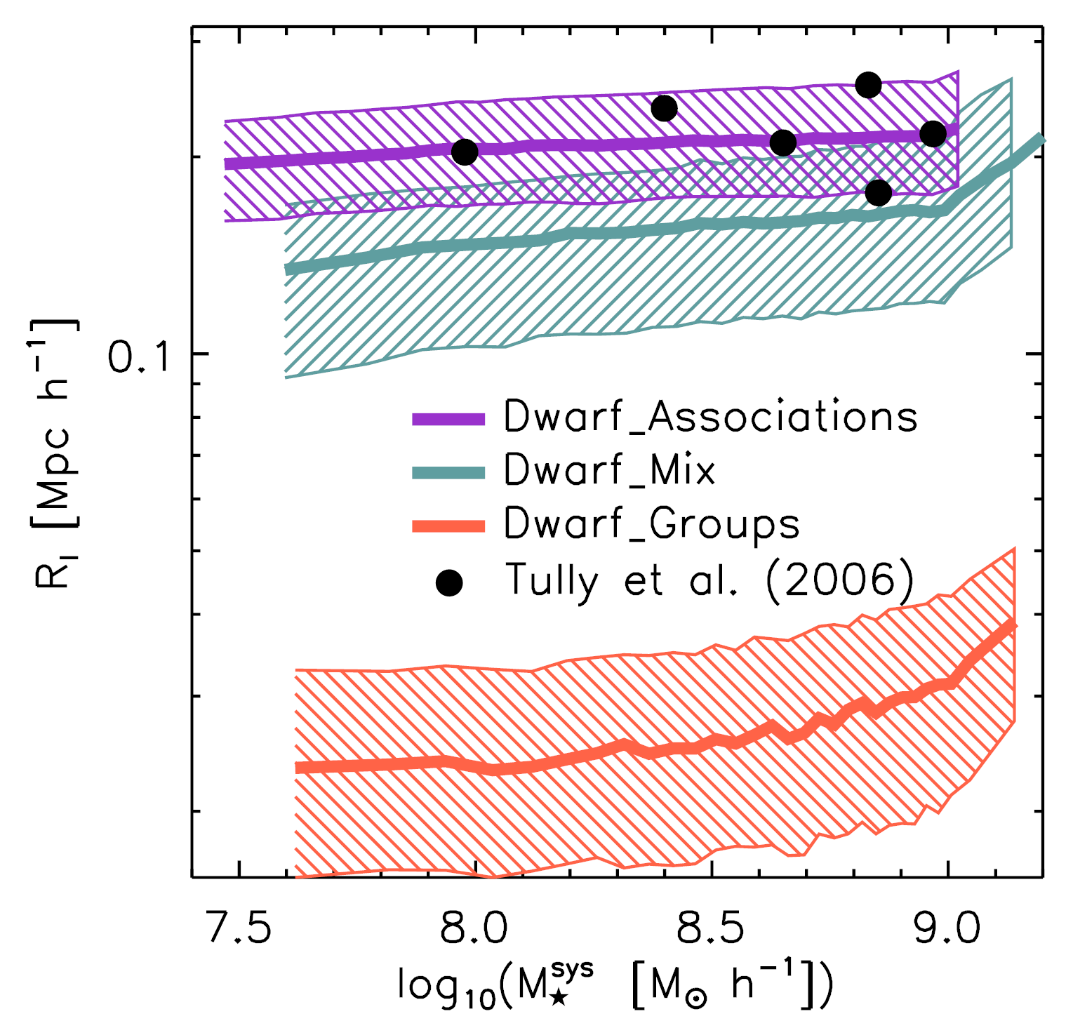
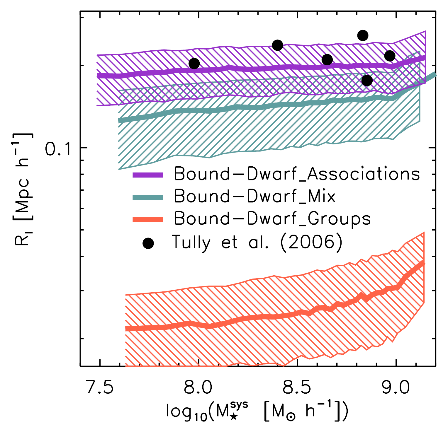
Figure 2: Left panel: Size of dwarf galaxy systems ($R_{I}$) as a function of the stellar mass of the system ($M_{\star}^{\rm sys}$). Different coloured lines correspond to different samples: Dwarf_associations (purple line), Dwarf_mix (green line) and Dwarf_groups (orange line). Solid lines show median values, taking equal number of bins in $M^{\rm sys}_{\star}$. Shaded regions cover from $25$ per cent to $75$ per cent for each sample. They are compared with observational results for dwarf galaxy associations taken from Tully et al. (2006, black filled circles), assuming for them a factor equal to one in the mass-to-light ratio. Rigth panel: Idem as left panel but considering sub–samples of only gravitationally bound systems: Bound–Dwarf_associations (purple line), Bound–Dwarf_mix (green line) and Bound–Dwarf_groups (orange line).

The galaxy samples analyzed in this work are obtained from a set of semi-analytical galaxies built by enforcing a minimum stellar and halo mass of $M_{\star}=10^{6.8}\,{\rm M}_{\odot}\,h^{-1}$, and $M_{200}=10^{9.28}\,{\rm M}_{\odot}\,h^{-1}$ (equivalent to $20$ DM particles), respectively. The final sample has a total of $26\,506\,948$ well resolved, semi-analytical galaxies, with stellar masses ranging between $6.8<{\rm log_{10}}(M_{\star}[{\rm M}_{\odot}\,h^{-1}])<12.9$ and halo masses ranging between $9.28<{\rm log_{10}}(M_{200}[{\rm M}_{\odot}\,h^{-1}])<15.17$. A well-established percolation algorithm, known as friends-of-friends (FOF, Huchra & Geller, 1982), is used to identify galaxy systems with sizes similar to the observed associations presented in Tully et al. (2006). To define our samples, we follow the procedure described in Yaryura et al. (2020). We use a linking length of $0.4\,{\rm Mpc}\,h^{-1}$ and select systems of galaxies with at least 3 members. We select this linking length value following Yaryura et al. (2020) who analyze characteristic sizes of systems identified varying the linking length parameter between $0.3\,{\rm Mpc}\,h^{-1}$ and $0.5\,{\rm Mpc}\,h^{-1}$. Characteristic sizes of the systems are sensitive to the chosen linking length, being more extended when they use a greater linking length value. Comparing with the observational results presented by Tully et al (2006), they conclude that $0.4\,{\rm Mpc}\,h^{-1}$ is the best choice for the analysis of these associations. In a first instance, we do not include the velocity of the systems as a selection criteria since our main objective is to mimic observation. We want to identify systems with properties comparable to the observations, but considering the fewest possible restrictions in their selection.

As we are interested in systems made up only of dwarf galaxies, we remove those systems that have one (or more) galaxy member more massive than a stellar mass threshold $M_{\star,\rm max}$. In this paper, we consider dwarf galaxies as those galaxies less massive than $M_{\star,\rm max}=10^{9.0}$ ${\rm M}_{\odot}\,h^{-1}$ (we check that our results do not vary significantly if we consider a more restrictive value as $M_{\star,\rm max}=10^{8.5}$ ${\rm M}_{\odot}\,h^{-1}$, or a less restrictive value as $M_{\star,\rm max}=10^{9.5}$ ${\rm M}_{\odot}\,h^{-1}$). Once we selected systems made up only of dwarf galaxies, and following the classification made by Yaryura et al. (2020), we split the sample into three different sub-samples according to the following conditions: (i) systems with all their galaxy members belonging to the same main DM halo; (ii) systems with all their galaxy members belonging to different main host DM haloes; (iii) systems for which some of the galaxies belong to the same main DM halo, but others belong to different main host haloes. We refer to these respective sub-samples as: (i) Dwarf_groups, (ii) Dwarf_associations, and (iii) Dwarf_mix. It is important to note that each system belongs to only one of these sub-samples. For comparison, we also consider samples without restriction in the maximum value of the stellar mass of member galaxies. In those cases, the samples are called All_groups, All_associations, and All_mix, according to the previously described criterion of belonging to a DM halo. Table 2 summarises these samples.

Fig. 1 shows the spatial projected distribution of semi-analytical galaxies (small grey dots) in a slice of $10\,{\rm Mpc}\,h^{-1}$ thickness. Open purple circles show the position of the systems in the sample Dwarf_associations, while orange filled circles correspond to systems identified in the sample Dwarf_groups. To make the plot clearer, the circle radius indicates $5R_{\rm I}$, where $R_{\rm I}$ is the inertial radius considered as an indicator of the size of the system, defined by

$$R_{\rm I}=\left(\sum_{i}^{N}r_{i}^{2}/N\right)^{1/2},$$ (2)

where $r_{i}$ is the three–dimensional distance of a galaxy from the system centroid and the sum for each system is performed over all members ($N$). From this plot, it is evident that associations of dwarf galaxies, with all their galaxy members belonging to different main host DM haloes are much more numerous and noticeably larger than systems with all their galaxy members belonging to the same main host DM halo. It is expected that Dwarf_associations are more numerous than Dwarf_groups due to the resolution limit. Requiring a minimum halo mass of $M_{200}=10^{9.28}\,{\rm M}_{\odot}\,h^{-1}$, there are large number of dwarf galaxies that are not resolved and therefore are not taken into account. These ignored dwarf galaxies, which accompany the central galaxy of the main host halo, could form groups of dwarf galaxies that are dismissed in our analysis. However, although resolution effects can affect differently groups and associations, their relative abundance is not the main subject of our paper which focalizes in their dynamical and environmental properties.

Figure 3: Number of galaxy systems as a function of the number of members per system. Different coloured lines correspond to different samples: Dwarf_associations (purple line), Dwarf_mix (green line) and Dwarf_groups (orange line).

To identify which of the previously defined samples most accurately reproduces the observed data, we analyse different dynamical properties and attempt to match the observed size-stellar mass relation from Tully et al. (2006). Left panel of Fig. 2 shows the size of the systems ($R_{\rm I}$, defined in equation (2)) as a function of the stellar mass of the system ($M_{\star}^{\rm sys}$), defined as the sum of the galaxy stellar mass of all the galaxies defining each association or group. For comparison, we also plot the size of the observed dwarf galaxy associations taken from Tully et al. (2006) (black filled circles). This comparison is based on the B-band luminosity, $L_{B}$, of these observed systems, assuming a mass–luminosity ratio equal to 1. Notice that assuming a different value for the mass–luminosity ratio would only cause a horizontal shift in our results, which does not modify the conclusions. Systems in the sample Dwarf_associations do much better in reproducing the empirical characteristic sizes of the observational sample of dwarf galaxies associations, in agreement with the results presented by Yaryura et al. (2020). From this figure, it is evident that systems in the sample Dwarf_groups are systematically smaller than systems in the sample Dwarf_associations by a factor of $\sim 5$.

Associations presented by Tully et al. (2006) are systems identified from the spatial distribution of dwarf galaxies, so we do not have information regarding the full dynamics of these systems. As a next step and taking advantage of the information provided by simulations, we estimate the binding energy of our theoretical systems compound only by dwarf galaxies to deduce whether they are gravitationally bound. Then, we analyze subsamples of previously described samples (Dwarf_associations, Dwarf_mix and Dwarf_groups) considering only gravitationally bound systems. We estimate the binding energy of the systems by considering the contribution of each member galaxy, classifying a system as gravitationally bound if its binding energy is negative. For consistency, we name these sub–samples as Bound–Dwarf_associations (96902 systems, $\sim 31$ per cent of the original sample Dwarf_associations), Bound–Dwarf_mix (181046 systems, $\sim 70$ per cent of the original sample) and Bound–Dwarf_groups (39048 systems, $\sim 96$ per cent of the original sample). Right panel of Fig. 2 shows same as left panel but considering sub–samples of only gravitationally bound systems. There are no significant differences between both panels, indicating that the sample of Bound–Dwarf_associations show more similar results to the observational sample of dwarf galaxies associations, same as left panel.

It is evident that observed associations have characteristic sizes comparable with Dwarf_associations, from where we could infer that member galaxies of the observed associations would be located in different main DM haloes. Furthermore, if the observed associations were in the same DM halo, it would likely be a large halo (due to the extended size of these systems), making it unlikely that the central galaxy is a dwarf galaxy. Therefore, based on Fig. 2, henceforth we concentrate on the samples Dwarf_associations and its sub–sample Bound–Dwarf_associations to analyse how the environment affects their main dynamical properties. The rest of the samples are used for comparison.

Figure 4: Number of systems located in each large-scale environment classification: knot (red bars), filament (blue bars), wall (green bars) and void (magenta bars); for the samples Dwarf_associations (left panel), Dwarf_mix (middle panel) and Dwarf_groups (right panel). Percentage values with respect to the total of each sample are indicated above each bar.

To better understand whether galaxy members of Dwarf_associations are preferably central galaxies, satellite galaxies with DM substructure or orphan galaxies, we study the internal structure of these associations. We find that $90$ per cent of these systems are composed of 3 or 4 members, most of which are central galaxies ($\sim 97.5$ per cent) while the rest are orphan galaxies ($\sim 2.5$ per cent). Fig. 3 shows the number of galaxy systems as a function of the number of members per system. Different coloured lines correspond to different samples: Dwarf_associations (purple line), Dwarf_mix (green line) and Dwarf_groups (orange line). From this figure it is evident that most of the systems are composed just of 3 or 4 members: $90$ per cent for Dwarf_associations, $75$ per cent for Dwarf_mix and $98$ per cent for Dwarf_groups.

4 Environmental effects

4.1 Classification of the environment

In the last few years, many papers have found evidence of properties of galaxies and systems of galaxies that depend on the environment in which they reside (Dressler, 1980; Kauffmann et al., 2004; Blanton et al., 2005; O’Mill et al., 2008; Peng et al., 2010; Wetzel et al., 2012; Zheng et al., 2017; Wang et al., 2018; Duplancic et al., 2020, among others). There are many different methods to classify large-scale cosmic matter distribution (see Libeskind et al., 2018, for a review). Most of these define the Hessian matrix from the density, velocity or potential field using a fixed finite grid. Then, this matrix is diagonalised to determine their eigenvectors and eigenvalues, which give information about the principal directions and strength of local collapse or expansion. The main disadvantage of these methods is the finite resolution assigned by a finite grid. Wang et al. (2020) presented an improvement to these methods given by an adaptive interpolation guaranteeing higher resolution. We apply this method to our samples and refer the reader to Wang et al. (2020) for a detailed description of their method.

To characterise the environment where associations of dwarf galaxies are found, we use the eigenvalues estimated from both the tidal tensor (e.g. Hahn et al., 2007a) and shear velocity (Hoffman et al., 2012) of the DM particle distribution of the parent simulation smdpl. We define four types of environment: knot, filament, wall or void, based on the number of eigenvalues larger than a chosen threshold ($\lambda_{\rm th}$). If we adopt the nomenclature $\lambda_{1}<\lambda_{2}<\lambda_{3}$ for the smallest, intermediate and largest, respectively, then we define

1. Knot: if $\lambda_{\rm th}<\lambda_{1}$

2. Filament: if $\lambda_{1}<\lambda_{\rm th}<\lambda_{2}$

3. Wall: if $\lambda_{2}<\lambda_{\rm th}<\lambda_{3}$

4. Void: if $\lambda_{3}<\lambda_{\rm th}$

We use a grid of $400^{3}$ cells and three different specific smoothing lengths $l=1,\,2$ or 4 $\,{\rm Mpc}\,h^{-1}$ over the tidal and shear velocity tensor. Then, we estimate the three eigenvalues for each cell. According to the position of the centre of mass of each association, we assign to it the eigenvalues of the cell where it is located. Following Wang et al. (2020), we adopted a threshold $\lambda_{\rm th}=0$ to define the four classifications. In this way, each association belongs to a single environment: void, wall, filament or knot.

The distribution of associations among the different environments depends on the choice of the smoothing length, as shown in Appendix A. We have checked that the results obtained in this work do not depend either on the field used to classify the environment (tidal tensor or shear velocity), or on the smoothing length ($l=1,\,2$ or 4 $\,{\rm Mpc}\,h^{-1}$). Therefore, for simplicity and clarity, the results of this paper will be presented only for the tidal tensor and for the smoothing length $l=1\,{\rm Mpc}\,h^{-1}$. This smoothing length represents about 5 times the median size of the associations, so it is a sufficient volume to analyse their environment.

Note that taking $\lambda_{\rm th}=0$, this classification takes into account only the sign of the eigenvalues and not the ratio between the eigenvalues. Furthermore, the tidal tensor eigenvalues refer to the directions of differential motion, namely compression and expansion. This should not be confused with the ellipsoidal shape of the mass distribution, defined by the inertia tensor. In general, however, there is a correlation and an alignment between the inertia tensor and the tidal tensor eigenvalues (Porciani et al., 2002). A knot means that the three eigenvalues are pointing inwards, i.e. the system is collapsing; a filament means that 2 eigenvalues are collapsing and one expanding (the expansion direction corresponds to the filament’s ‘spine’). A wall means that 2 eigenvalues are expanding and one is collapsing (which corresponds to the sheet normal), and a void means that the three eigenvalues are pointing outwards, i.e. the system is expanding.

According to this large-scale environment classification (knot, filament, wall, void), most of the associations in the Dwarf_associations sample are located in filaments ($\sim 67$ per cent), followed by the wall environment ($\sim 26$ per cent), while a minority fraction is in knots ($\sim 6$ per cent) and voids ($\sim 1$ per cent). We specify percentage values for systems with all their galaxy members belonging to different main host DM haloes, i.e. the Dwarf_associations sample, because they are the focus of our work, but these values do not change significantly for other samples. Fig. 4 shows the number of systems located in each large-scale environment classification, for the samples Dwarf_associations, Dwarf_mix and Dwarf_groups (percentage values are indicated above each bar). For the rest of the samples, these values do not change significantly either. For example, for the All_associations sample, $\sim 69$ per cent of the systems are located in filaments, $\sim 24.5$ per cent in walls, $\sim 6$ per cent in knots, and only $\sim 0.5$ per cent in voids. Likewise, if we consider systems without a restriction in the maximum value of the stellar mass of their member galaxies and without distinction of the halo in which their member galaxies are hosted (i.e. All_associations + All_mix + All_groups), the percentages are very similar: $\sim 70$ per cent in filaments, $\sim 22$ per cent in walls, $\sim 7.5$ per cent in knots, and $\sim 0.5$ per cent in voids. Although it is not a strictly direct comparison, we can compare these percentages with the mass fraction assigned to a given environmental classification. As we have already mentioned above, a variety of methods have been developed to classify the cosmic web (see Libeskind et al., 2018, for a review). As these methods identify the web components differently, it is not surprising that there are significant discrepancies in these fractions. Despite these differences, for most of these methods, the largest mass fraction is found in filaments (ranging from $\sim 30$ to $\sim 90$ per cent depending on the method), followed by walls or nodes depending on the method, while the lowest mass fraction is found in voids (less than 10 per cent in most of these methods). Despite not being a direct comparison and taking into account the differences in the percentages, our results follow the same trend presented by these works.

Figure 5: Values of the three eigenvalues as a function of the stellar mass of associations for the sample Dwarf_associations split according to the environment in which they reside as indicated by the legends. Coloured solid lines show median values of eigenvalues taking equal number of bins in $M_{\star}^{\rm sys}$. Shaded regions cover from $25$ per cent to $75$ per cent for each sample.

Fig. 5 shows values of the three eigenvalues as a function of the total stellar mass of the systems ($M_{\star}^{\rm sys}$), for the sample Dwarf_associations, split according to the environment in which they reside as indicated by the legends. Coloured lines show median values of eigenvalues taking equal number of bins in $M_{\star}^{\rm sys}$, while shaded regions cover from $25$ per cent to $75$ per cent for each sample. The eigenvalues do not show a significant dependence on the stellar mass of the association. From this figure, the sign of each eigenvalue is evident, indicating the direction of the tidal field (collapse if positive and expansion if negative) taking into account the adopted threshold $\lambda_{\rm th}=0$ for the classification of the structure in the cosmic web.

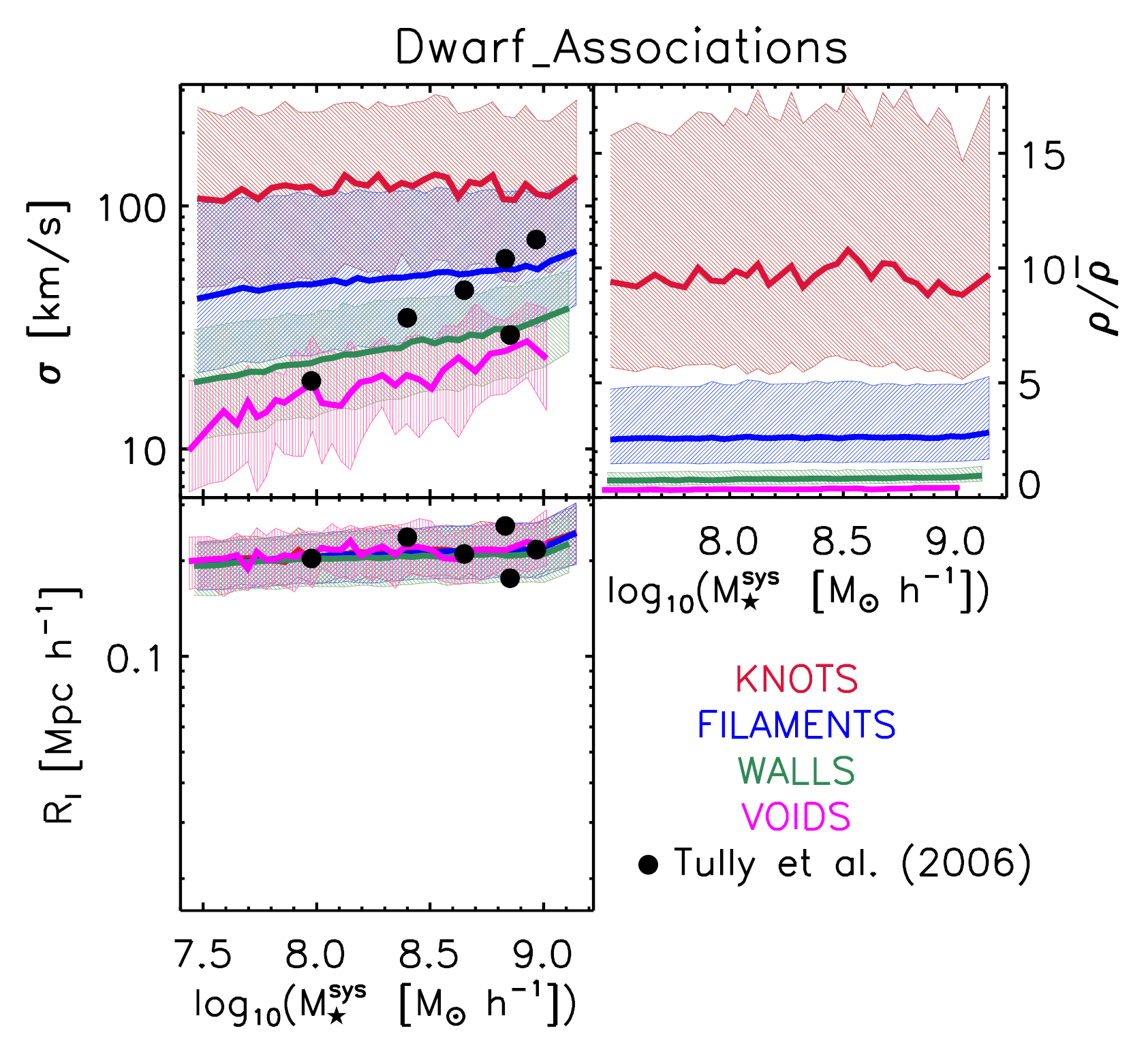
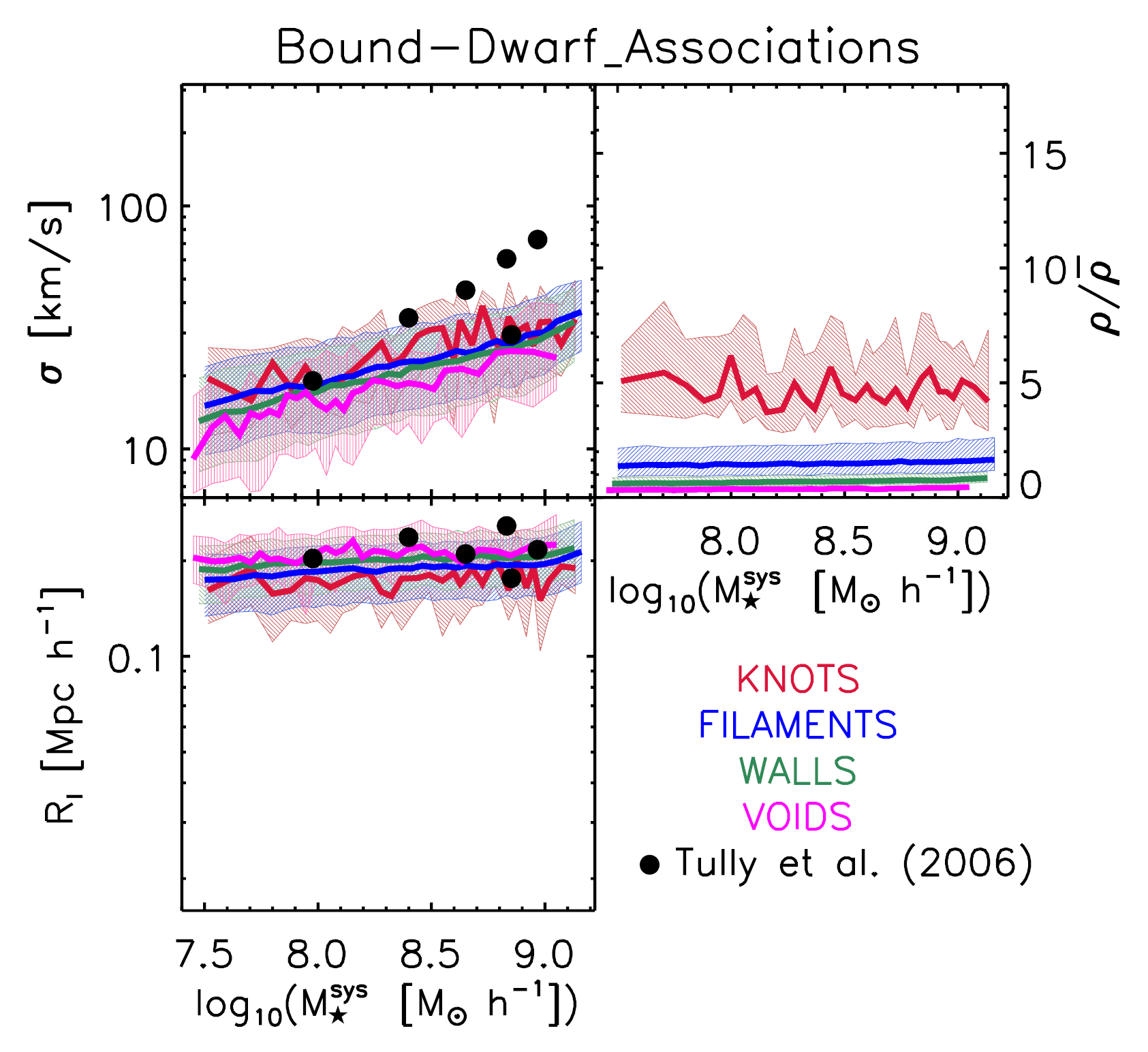
Figure 6: Left panels: Dynamical properties of associations as a function of the stellar mass of the association ($M_{\star}^{\rm sys}$) for systems in the sample Dwarf_associations: velocity dispersion ($\sigma$, top left), size ($R_{\rm I}$, bottom left) and the ratio between the DM particles density $\rho$ in the grid cell where the system is located and the mean density ($\rho/\bar{\rho}$, top right). Solid lines show median values of each property, taking equal number of bins in $M_{\star}^{\rm sys}$. Each colour corresponds to a different environment (knots, filaments, walls and voids) as indicated in the legends. Shaded regions cover from $25$ per cent to $75$ per cent for each sample. Results for simulated associations of dwarf galaxies are compared with observational results taken from Tully et al. (2006, black filled circles), assuming for the latter a factor equal to one in the mass-to-light ratio. Rigth panels: Idem as left panels but considering a sub–sample with only gravitationally bound systems (Bound–Dwarf_associations).

4.2 Properties of dwarf galaxy associations

To analyse the environmental effects on the associations of dwarf galaxies, we study how their main dynamical properties vary according to the environment in which these particular systems reside. As the main intrinsic properties of our systems, we compute the inertial radius ($R_{\rm I}$, defined in eq. (2)) as an indicator of the size of the system, the velocity dispersion ($\sigma$), and the stellar mass of the system ($M_{\star}^{\rm sys}$). The velocity dispersion is computed through the unbiased sample variance of the sample for all member galaxies, defined by

$$\sigma=\left[\sum_{i}^{N}v_{i}^{2}/(N-1)\right]^{1/2}.$$ (3)

where $v_{i}$ is the one-dimensional velocity difference between a galaxy and the mean velocity of the system.

Fig. 6 shows the main dynamical properties of our systems ($R_{\rm I}$ and $\sigma$) as a function of the total stellar mass of the association ($M_{\star}^{\rm sys}$) for systems in the sample of dwarf galaxy associations (Dwarf_associations, left panels). Coloured lines show median values of each property taking an equal number of bins in $M_{\star}^{\rm sys}$. Each colour corresponds to a different environment (knots, filament, walls and voids), as indicated by the legends. Top right panels show the ratio between the DM particles density $\rho$ in the grid cell where the system is located and the mean density ($\rho/\overline{\rho}$) as a function of the stellar mass of the system. This ratio is related with eigenvalues by $\rho/\overline{\rho}-1=\lambda_{1}+\lambda_{2}+\lambda_{3}$. As expected, it is clear that knots correspond to the highest densities, followed by filaments, then walls and finally voids, which correspond to the lowest density. From the results for the associations (Dwarf_associations sample), it is evident that the velocity dispersion depends strongly on the environment where the association is located. Associations have a very low velocity dispersion ($\sigma\sim 20\,{\rm km\,s^{-1}}$) if found in voids, which increases up to $\sigma\sim 140\,{\rm km\,s^{-1}}$ as we move to knots, going through walls and filaments. As associations are composed exclusively of galaxies that do not live in the same DM halo, they are somehow tracing the velocity dispersion of the environment where they are located: knot, filament, wall or void. This dependence of velocity dispersion on the environment has already been previously studied in some published works. Among the most recent, we can mention Taverna et al. (2023) who study the effects of different global environments on the properties of Hickson-like compact groups of galaxies (CGs) identified in the Sloan Digital Sky Survey Data Release 16 (Ahumada et al., 2020). They found that CG velocity dispersion increases with the density of the environment they inhabit, since the median velocity dispersion observed for CGs in the highest-density environments almost doubles that observed for CGs in the lowest-density environments. Furthermore, we can mention the results presented by Ruiz et al. (2019) who compare pairwise velocity ($w$) distributions for all galaxies with pairwise velocity distributions for galaxies located in void regions. They found $w\sim 500\,{\rm km\,s^{-1}}$ for all galaxies, while for void galaxies the pairwise velocity dispersions are in the range $w\sim 50-70\,{\rm km\,s^{-1}}$, roughly one order of magnitude smaller. They found these differences in both the observations and in the simulated galaxies. Our results are in accordance with these results in the sense that the velocity dispersion shows the same trend, being significantly smaller in low-density regions than in high-density regions. Moreover, this progressive increase of the values of the velocity dispersion through different environments, regardless of the total stellar mass of the association, is also accompanied by an increasing trend of the velocity dispersion with increasing $M_{\star}^{\rm sys}$, and this trend is more pronounced for associations residing in filaments and almost non-existent in associations located in knots. In relation to the size of the associations, there are no systematic effects of the environment on the size of associations.

Compared with observational results, the dynamical properties of most of the observed dwarf galaxy associations presented by Tully et al. (2006) (black filled circles) are compatible at first glance with a filament-like (3 systems) or wall-like (2 systems) environment, while just 1 association is compatible with a void-like environment. In a deeper analysis, we compute the probability of each association to belong to a web-type environment classification. We estimate the probability distribution function (PDF) of velocity dispersion for each web-type environment classification, regarding bins of mass. Taking this distribution into account we assign a probability value for each observed association. This probability is shown in Table 3, where the highest probability for each association is highlighted in bold type. The associations are stored in increasing order of their velocity dispersion. Considering the highest values of these probabilities, it appears that two associations belong to the void-like environment (Association 1 and Association 2), two belong to the wall-like environment (Association 3 and Association 4), and two belong to the filament-like environment (Association 5 and Association 6). Nevertheless, these highest probabilities are not significantly larger compared to the others, thereby indicating that the membership in a given web-type classification is not particularly evident. This is primarily due to the large scatter in velocity dispersion for each environment, as evidenced by the shaded regions in the figure. Another important thing to note is that, as the velocity dispersion of the associations increases, the probability of belonging to denser environments also increases.

We also analyze systems in the sample built without restriction in the maximum value of the galaxy stellar mass (All_associations) and there are not significant differences between their results and those previously described. Due to the similarities between results, we do not show the latter ones to make the discussion clearer. In brief, these results show that the increase of $\sigma$ with the density of the environment does not happen only in associations of dwarf galaxies, but is noticed in all systems where their member galaxies belong to different DM haloes.

Observed	$\sigma[{\rm km/s}]$	Knot	Filament	Wall	Void
Associations
1	19.05	6$\%$	16$\%$	34$\%$	44$\%$
2	29.44	6$\%$	21$\%$	33$\%$	40$\%$
3	34.64	10$\%$	26$\%$	36$\%$	28$\%$
4	45.03	17$\%$	30$\%$	32$\%$	20$\%$
5	60.62	24$\%$	35$\%$	29$\%$	12$\%$
6	72.75	34$\%$	39$\%$	27$\%$	0$\%$

Table 3: Probability of each observed association to belong to one environment. First column indicates the association. Second column shows the velocity dispersion of the association. Third, fourth, fifth and sixth columns indicate the probability of each observed association to belong to one web type environment: knot, filament, wall and void, respectively. The highest probability for each association is highlighted in bold type.

Going even further, right panels of Fig. 6 show the same as left panels but considering only gravitationally bound systems (Bound–Dwarf_associations). For this sample, it is evident that the dependence of velocity dispersion on the environment where the association is located is noticeably attenuated. The velocity dispersion covers a narrow range around low velocity dispersions, between $\sigma\sim 10\,{\rm km\,s^{-1}}$ and $\sigma\sim 30\,{\rm km\,s^{-1}}$, depending on the mass of the system, with minimal differences according to the environment in which they are located. Although a trend is slightly visible, it is too weak. Therefore, we can infer that the velocity dispersion of gravitationally bound systems does not depend on the environment in which they reside. Comparing with observational results, the velocity dispersion of at least half of the observed dwarf galaxy associations presented by Tully et al. (2006) (black filled circles) are not compatible with our results. This would indicate that these observed associations could be non–gravitationally bound systems.

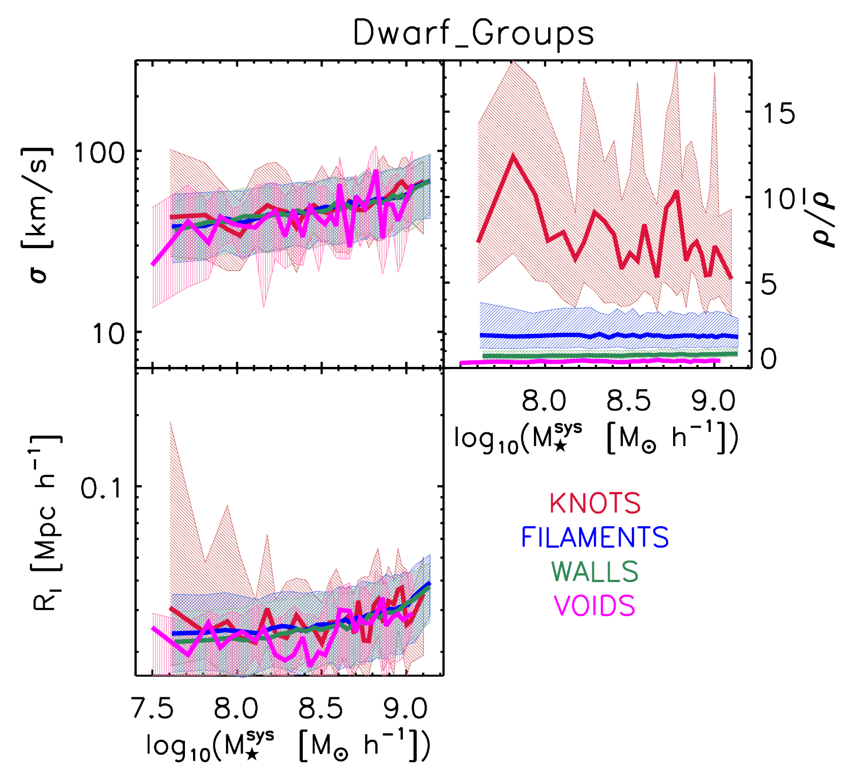
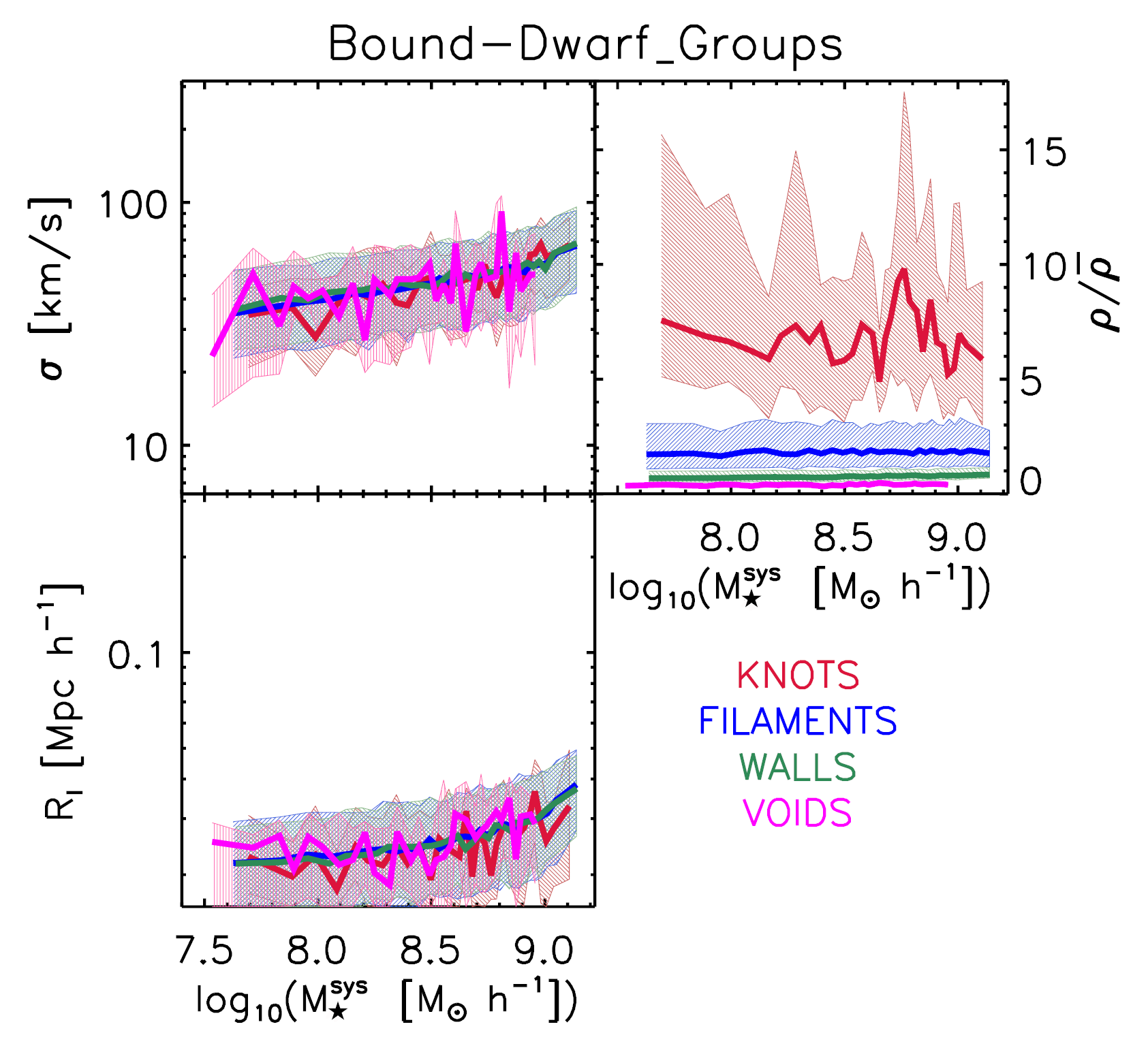
Figure 7: Left panels: Dynamical properties of groups of galaxies as a function of the stellar mass of the group ($M_{\star}^{\rm sys}$) for systems in the sample Dwarf_groups: velocity dispersion ($\sigma$, top left), size ($R_{\rm I}$, bottom left) and the ratio between the DM particles density $\rho$ in the grid cell where the system is located and the mean density ($\rho/\bar{\rho}$, top right). Solid lines show median values of each property, taking an equal number of bins in $M_{\star}^{\rm sys}$. Each colour corresponds to a different environment (knots, filaments, walls and voids) as indicated in the legends. Shaded regions cover from $25$ per cent to $75$ per cent for each sample. Rigth panels: Idem as left panels but considering a sub–sample with only gravitationally bound systems: Bound–Dwarf_groups.

Fig. 7 shows the same relationships as Fig. 6 but considering different samples. Panels in the left box correspond to systems of sample Dwarf_groups while panels in the right box correspond to systems of sample Bound–Dwarf_groups, a sub–sample of the former containing only gravitationally bound systems. In these cases, unlike the samples shown in the previous figure, all member galaxies belong to the same main host DM halo. It is noticeable that the typical size of these systems is much smaller than those of samples Dwarf_associations and Bound–Dwarf_associations shown in Fig. 6. Moreover, the dependence of $\sigma$ on the environment in which the systems reside disappears. It is evident that the behaviour of $\sigma$ with respect to the stellar mass of the system is very similar for all environments. As expected, the results of these two samples are very similar between them, due to the fact that Bound–Dwarf_associations is a sub–sample of Dwarf_groups, which contains about $\sim 96$ per cent of their groups. The remaining $\sim 4$ per cent, that is, the unbound groups of dwarf galaxies, mainly consist of subgroups found within larger DM halos. We also analyze systems in the sample built without an upper limit in their stellar mass (All_groups) and there are not significant differences between their results and those just described. Again, we avoid showing the results of this sample for a less confusing discussion. So, in summary, velocity dispersion does not depend on the environment when all galaxy members of the system belong to the same main DM halo.

Comparing results from Figs. 6 and 7, we infer that, when estimating the velocity dispersion $\sigma$ for systems that belong to the Dwarf_associations sample, we are actually estimating the velocity dispersion of the environment in which the associations are immersed, immediately surrounding them, and not of the system itself. Since galaxy members of these systems belong to different main DM haloes, they are located far from each other. When estimating velocity dispersions of a set of galaxies that are far away from each other, the properties of the environment inevitably affect this estimation. This occurs not only for associations of dwarf galaxies, but for all systems where all their member galaxies belong to different main DM haloes (Dwarf_associations and All_associations samples). In contrast, when we consider gravitationally bound systems, the difference in the velocity dispersion with the environment is noticeably attenuated, completely disappearing if we consider systems where all their member galaxies belong to the same main DM halo. This is true for systems built up only of dwarf galaxies and for systems without restriction in the stellar mass of their member galaxies, i.e., Bound–Dwarf_associations, Bound–Dwarf_groups, Dwarf_groups and All_groups samples. In summary, considering systems whose galaxies belong to the same main DM halo or gravitationally bound systems (despite the fact that their member galaxies may belong to different main DM haloes), the environment does not play a fundamental role when we estimate the velocity dispersion of their member galaxies. The size of dwarf galaxy systems are directly related to the DM halo in which galaxies reside, while the velocity dispersion of dwarf galaxy systems are directly related to the binding energy of the system and not to the environment in which the DM halo is found within the cosmic web.

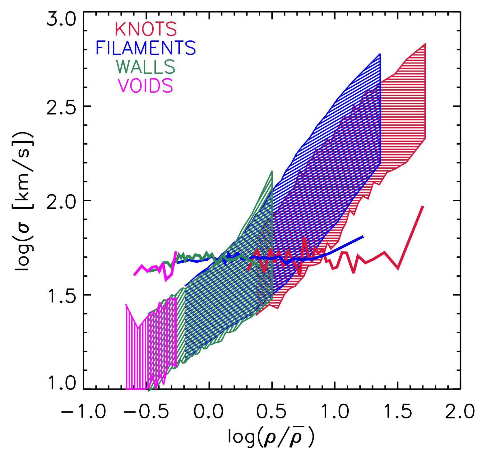
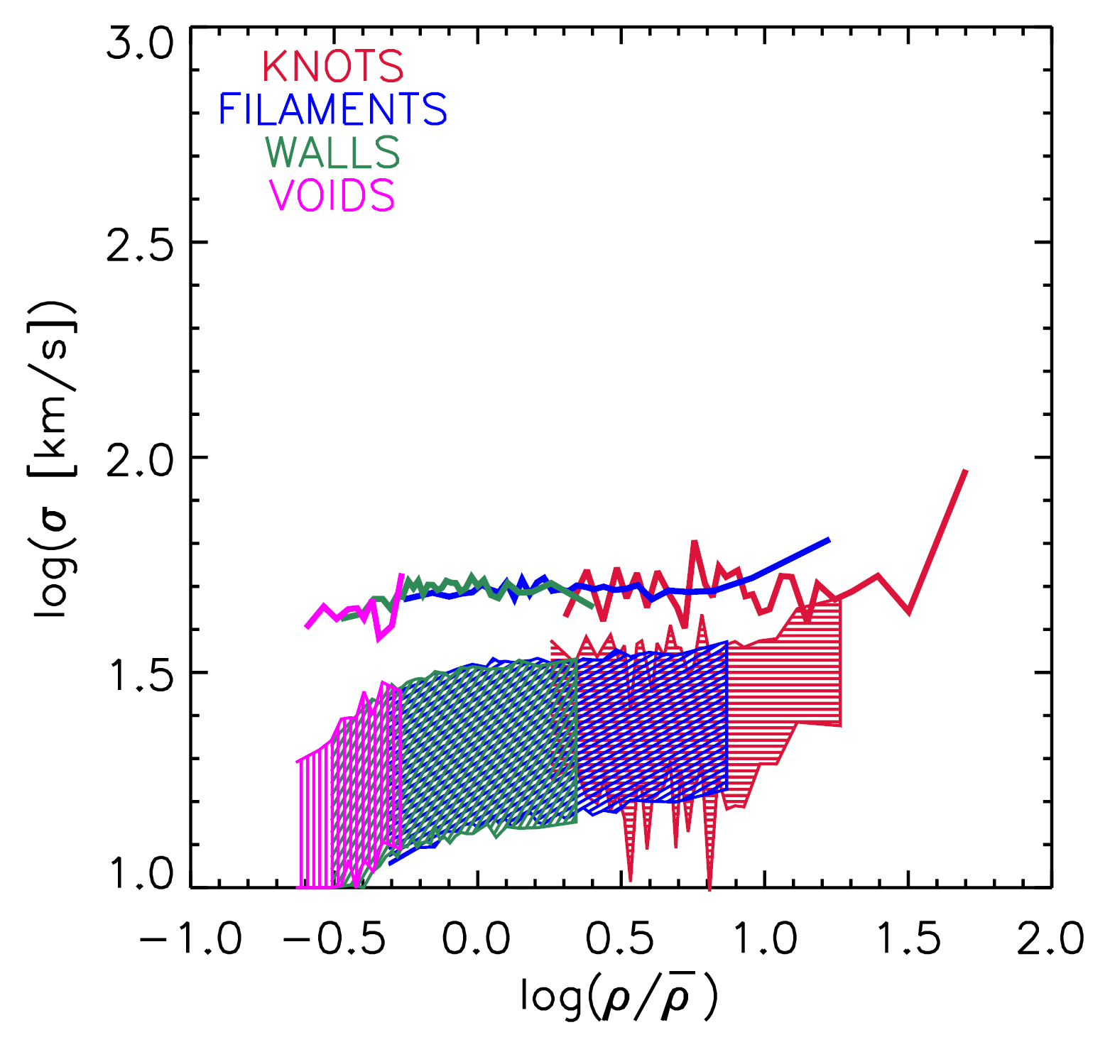
Figure 8: Left panel: Velocity dispersion ($\sigma$) as a function of DM particle density $\rho$ in the grid cell where the system is located divided by the mean density ($\rho/\bar{\rho}$), shown for two different samples, Dwarf_associations (shaded regions) and Dwarf_groups (solid lines), for four different environments, as indicated by the colour code. Shaded regions cover from $25$ per cent to $75$ per cent for the Dwarf_associations sample. For the case of Dwarf_groups, we show only the median values (i.e. corresponding to $50$ per cent of the sample) to make the plot clearer. Rigth panel: Idem as left panel but considering sub–samples with only gravitationally bound systems: Bound–Dwarf_associations and Bound–Dwarf_groups.

The results that we have just reached can be better visualized by Fig. 8. Here, the velocity dispersion ($\sigma$) of the galaxy system as a function of the density field of the environment normalised by the mean density ($\rho/\bar{\rho}$) is shown for different samples. Left panel shows Dwarf_associations (shaded regions) and Dwarf_groups (solid lines) samples, residing in different environments (indicated by the colour code). Shaded regions cover from $25$ per cent to $75$ per cent of each sample of associations of dwarf galaxies; for dwarf groups, we show only median values (i.e., corresponding to $50$ per cent of the sample) to make the figure clearer. In the case of Dwarf_associations, the dependence of the velocity dispersion on density is remarkable. As the density of the system environment increases, the velocity dispersion of the system also increases. On the other hand, it is clear that the velocity dispersion of Dwarf_groups does not depend on the density of the environment in which the system resides. As the density of the system environment increases, the velocity dispersion does not show significant changes. This shows that the velocity dispersion of a system where all its member galaxies belong to different main DM haloes depends strongly on the environment in which the system is located. In contrast, the velocity dispersion of a system where all its member galaxies belong to the same main DM halo does not depend on the environment of the system. On the other side, right panels show samples where all systems are gravitationally bounded: Bound–Dwarf_associations (shaded regions) and Bound–Dwarf_groups (solid lines) samples. This comparison shows that velocity dispersion does not significantly depend on the environment when we restrict our samples to gravitationally bound systems. This figure confirms that the velocity dispersion of dwarf galaxy systems are directly related to the binding energy of the system and not to the environment in which the DM halo is found within the cosmic web, regardless whether member galaxies are hosted by the same main DM halo or by different main DM haloes.

5 Conclusions

We analyze how the dynamical properties of associations of dwarf galaxies depend on their environment. Within the $\Lambda$CDM cosmological context, we identify these particular systems in the high-resolution dark matter-only smdpl simulation (Klypin et al., 2016), coupled to the sag semi-analytical model of galaxy formation (Cora et al., 2018). We compare associations of dwarf galaxies, where all their members belong to different main DM haloes, with close groups of dwarf galaxies hosted by a single massive DM halo. From Yaryura et al. (2020) we know that the so defined associations of dwarf galaxies are the systems which best reproduce the dynamical properties of observed associations presented by Tully et al. (2006). That is why studying associations of dwarf galaxies is our main objective.

We classify the environment into the four different categories of knots, filaments, walls and voids, and analyse its effect on the main properties of the associations and groups of dwarf galaxies. Most dwarf galaxies associations are located in filaments ($\sim 67$ per cent), followed by walls ($\sim 26$ per cent), knots ($\sim 6$ per cent) and voids ($\sim 1$ per cent). So far, only seven associations of dwarf galaxies have been observed (Tully et al., 2006). Based on the observed velocity dispersion we conclude that three of them are most compatible with a filament-like environment, two with a wall-like environment, while just one is most compatible with a void-like environment. Based on the PDF of the velocity dispersion of associations in different environments we estimated the probabilities of the observed associations to be located in a specific environment (Table 3) and found that they tend to be located in low density environment (voids, walls up to filaments) and most probably cannot be found in knots. It is worth noting that as the velocity dispersion of the associations increases, so does the probability of belonging to denser environments.

When we analyze the dependence of the dynamical properties of the associations of dwarf galaxies on the environment, we find that the velocity dispersion strongly depends on the environment. Associations have a very high-velocity dispersion ($\sigma\sim 140\;{\rm km\,s^{-1}}$) if located in knots, which decreases to $\sigma\sim 20\;{\rm km\,s^{-1}}$ as we reach voids, going through filaments and walls. This dependency occurs in systems composed exclusively of dwarf galaxies as well as in systems with no restriction on the maximum value of the stellar mass of their member galaxies. Since the members of the associations belong to different DM haloes, these galaxy systems could be considered as large-scale mass distribution tracers. The velocity dispersion of these galaxies reflects the velocity dispersion of the environment (knot, filament, wall or void) in which they reside. Therefore large-scale environment plays a fundamental role in determining the dynamical properties of associations.

Being more restrictive in the definition of associations, requiring them to be gravitationally bound systems, our results change significantly. When we consider a sub–sample of associations of dwarf galaxies, with only gravitationally bound systems ($\sim 30$ per cent of the total sample of associations of dwarf galaxies), the dependence of the velocity dispersion on the environment is strongly attenuated. This indicates that the environment significantly influences the dynamical properties of systems only when they are not physically bound systems. Comparing with observational results presented by Tully et al. (2006), the velocity dispersion of most of these associations is not compatible with that of the bound systems, which could indicate that these observed associations would not be gravitationally bound systems.

When we focus on the groups of dwarf galaxies, defined as systems where all member galaxies belong to the same main DM halo, we do not find any dependence of the velocity dispersion on the environment. About $\sim 96$ per cent of the groups are gravitational bound systems. So, the dynamical properties of these groups are not influenced by the environment where they reside.

Data availability

The data underlying this article will be shared on reasonable request to the corresponding author.

Appendix A Stability of classification of environment

	TIDAL
	$l=1$	$l=2$	$l=4$
KNOTS	17671	28087	34667
FILAMENTS	206839	182974	165609
WALLS	81407	91564	98662
VOIDS	2333	5625	9312

Table 4: Number of dwarf galaxy associations in different environments (knots, filaments, walls, voids) estimated from the tidal tensor for three different values of smoothing length, $l=1,2$ and 4 $\,{\rm Mpc}\,h^{-1}$.

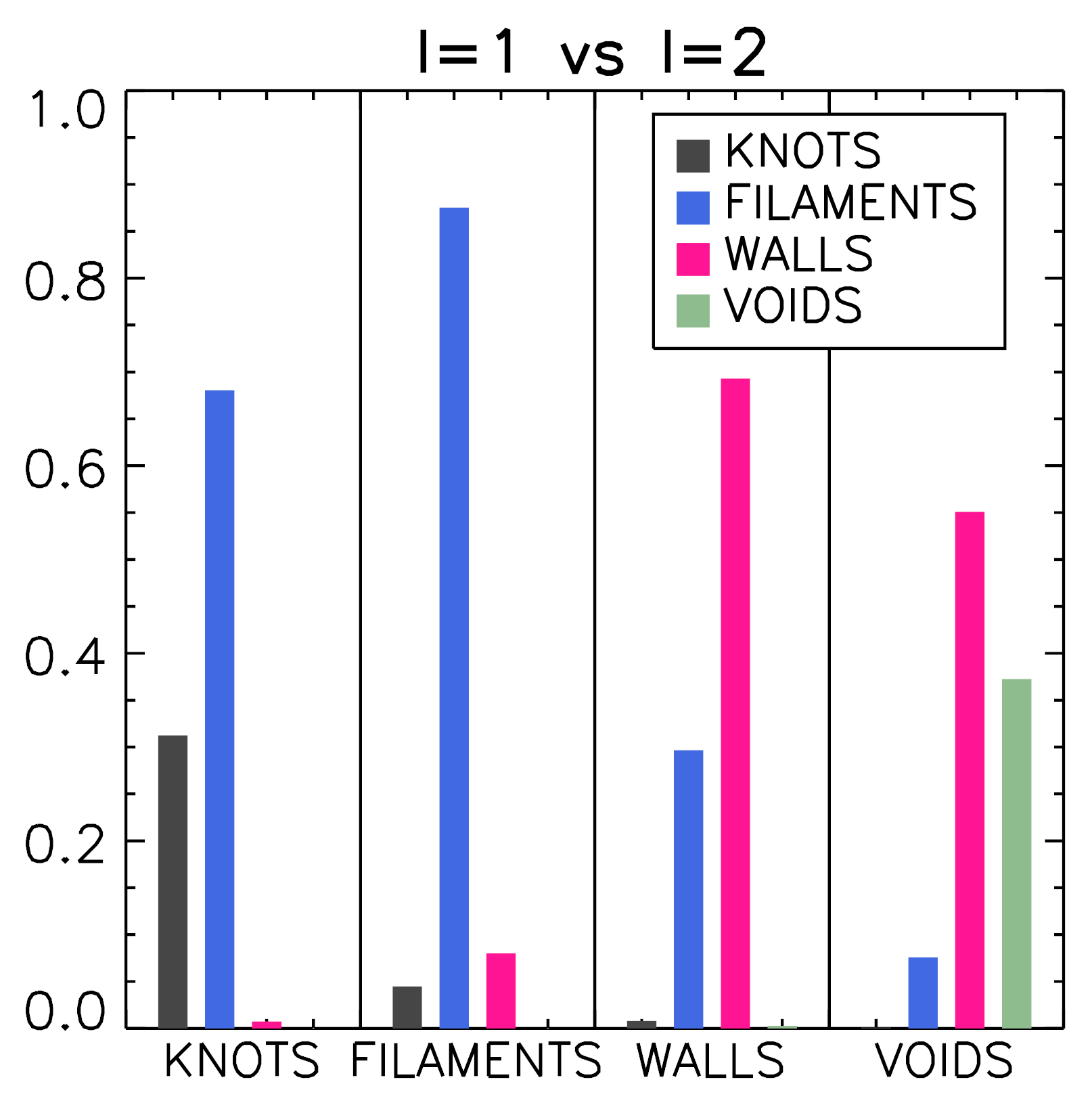
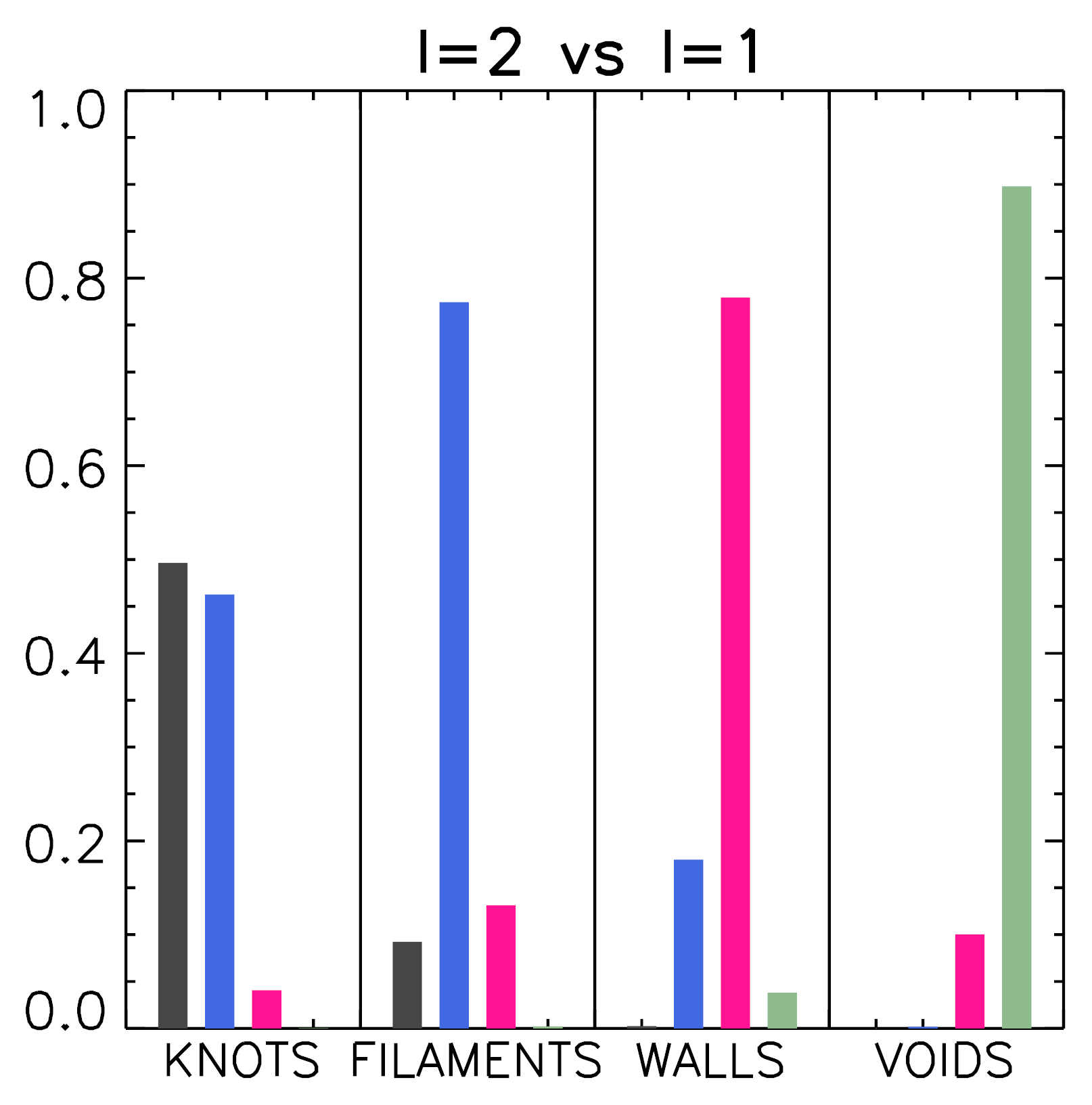
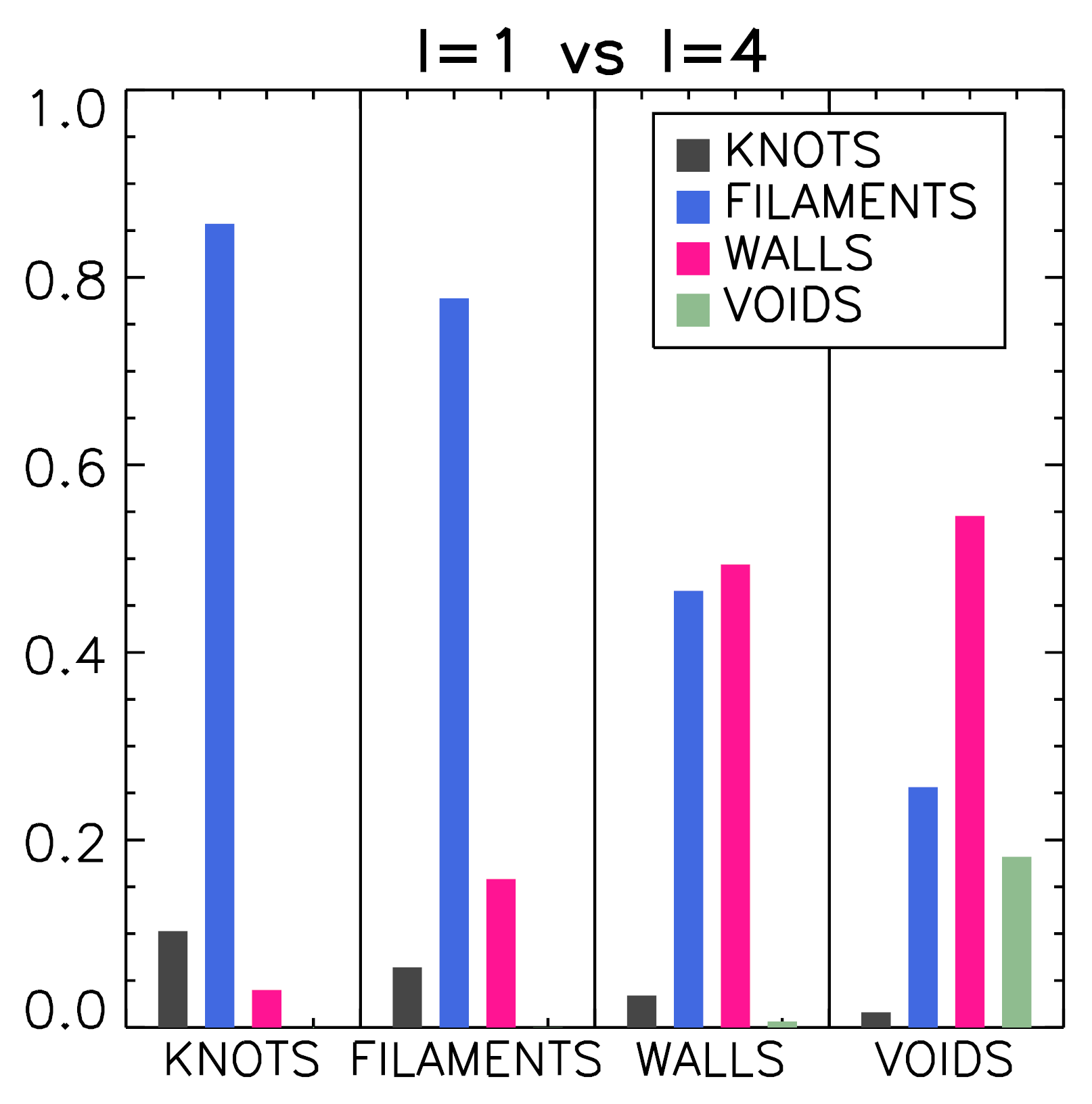
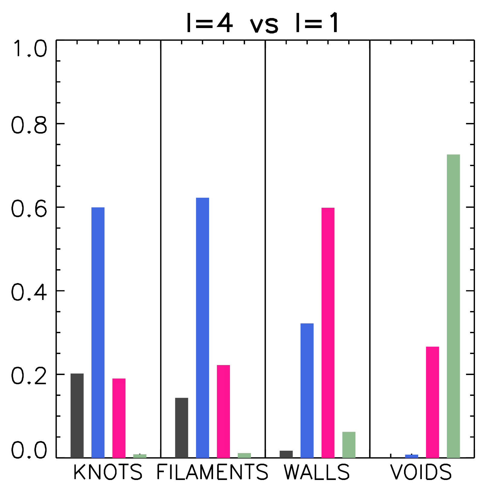
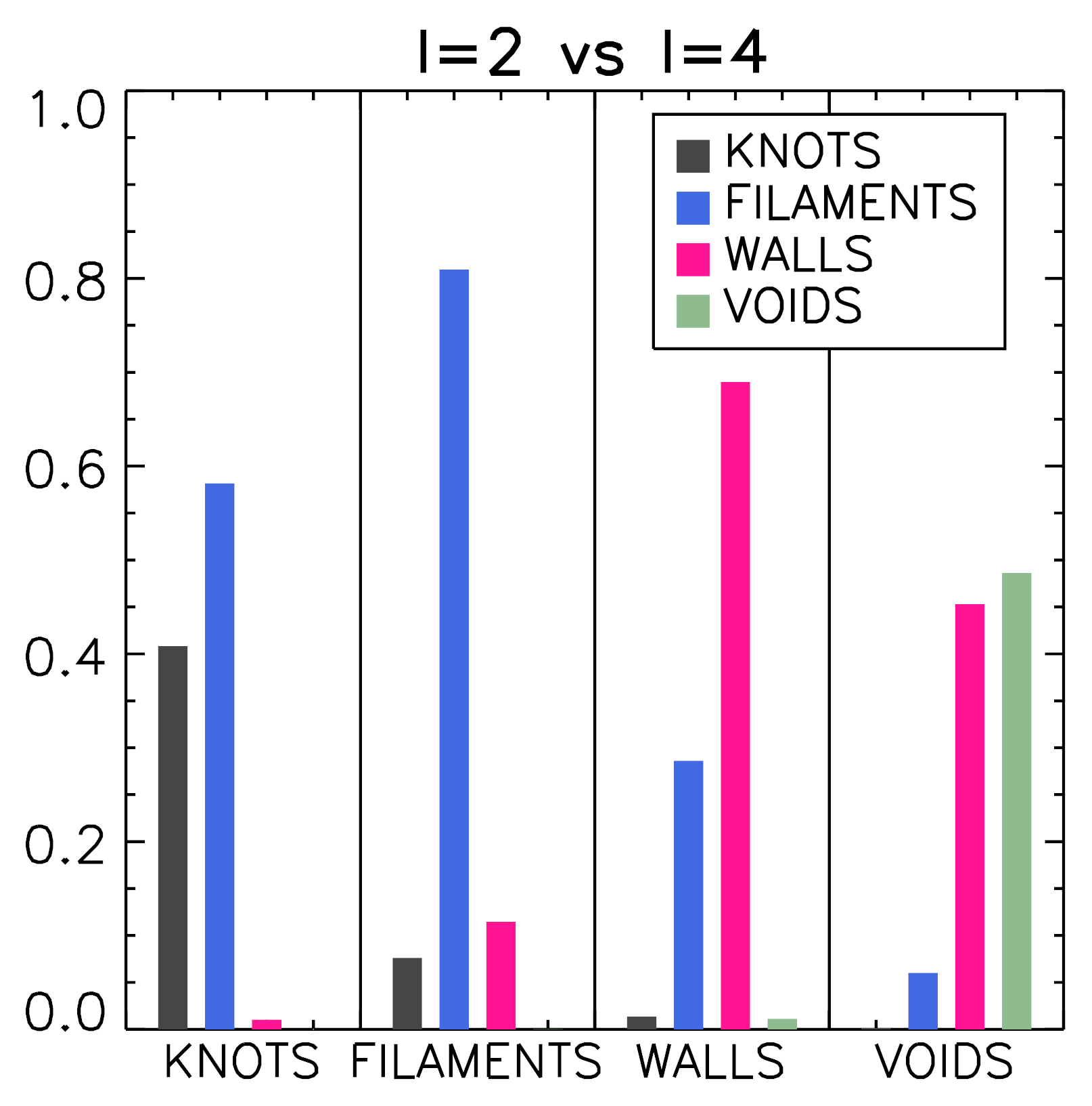
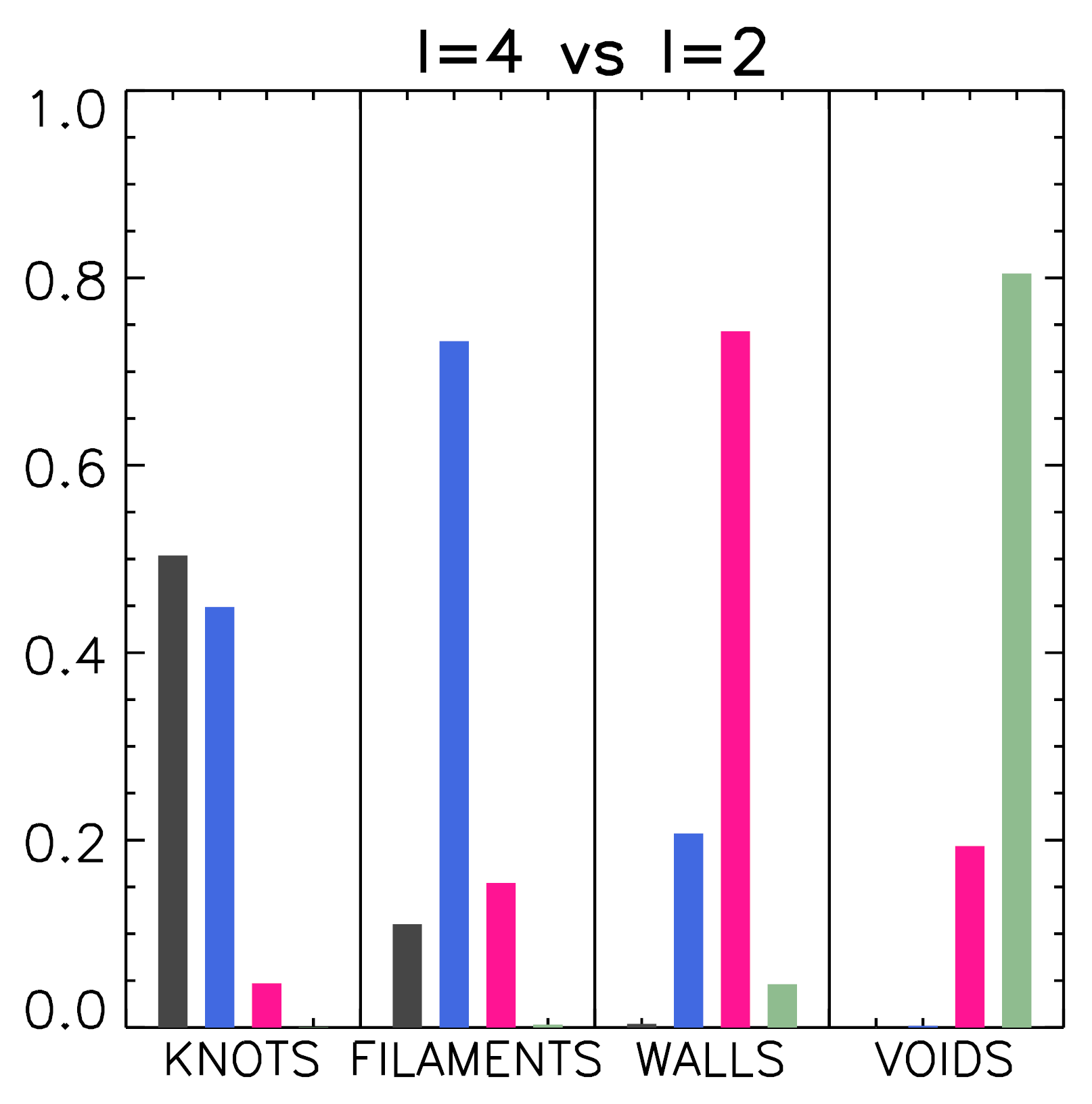
Figure 9: Change of associations from one category (knot, filament, wall or void) to another according to the smoothing length used to estimate the eigenvalues, comparing 2 samples at a time. Upper, middle and lower panels show the comparison between $l=1$ vs. $l=2$, $l=1$ vs. $l=4$ and $l=2$ vs. $l=4$ and their reciprocals, respectively, as indicated by legends.

In this appendix, we analyse the robustness of our classification scheme of the large–scale matter distribution of the cosmic web according to the variation of the characteristic scale adopted to estimate the density of the environment. In particular, we evaluate how the number of associations categorised in a given environment (knot, filament, wall or void) varies when changing the smoothing length ($l=1,2$ or 4 $\,{\rm Mpc}\,h^{-1}$). These four categories are assigned according to the sign of the eigenvalues of the Hessian matrix estimated from the gravitational potential (see Section 4.1). To compute these eigenvalues, first, the full simulated box of the smdpl simulation (described in Section 2.1) is covered with a fixed grid of $400^{3}$ cells. Then, the DM particle overdensity is smoothed using a spherically symmetric Gaussian window function with a given $l$, and the gravitational potential is estimated. The gravitational potential ($\phi$) is normalised by $4\pi G\overline{\rho}$ whereby it satisfies the Poisson equation ($\bigtriangledown^{2}\phi=\delta$), where $\delta$ is the dimensionless matter overdensity, $G$ the gravitational constant and $\overline{\rho}$ is the average density of the Universe. The Hessian matrix is constructed from this peculiar gravitational potential (tidal tensor) and we assign its three eigenvalues to each cell. Finally, we assign to each association the same eigenvalues as those of the cell in which the association centre is located. As expected, these eigenvalues depend on the $l$ of the Gaussian filter. For a given $l$, the number of eigenvalues greater than a given threshold ($\lambda_{\rm th}=0$) is used to classify the type of environment where each association resides: knot, filament, wall or void. Table 4 presents the number of dwarf galaxy associations in each environment for the three different smoothing lengths.

Fig. 9 shows how systems are identified as part of one environment (knot, filament, wall or void) or another according to the $l$ used. The upper, middle and lower panels show the comparison between $l=1$ vs. $l=2$, $l=1$ vs. $l=4$ and $l=2$ vs. $l=4$ and their reciprocals, respectively, as indicated by the legends. On the x-axis of each panel, there are four boxes corresponding to knots, filaments, walls and voids. In each of the boxes, there are four bars with different colours identifying knots (black), filaments (blue), walls (magenta) and voids (green). The length of each bar corresponds to the ratio $N_{XY}/N_{Y}$, where $N_{XY}$ is the number of objects belonging to category $X$ in, for example, $l=1$ but categorised as $Y$ in, for example, $l=2$, while $N_{Y}$ is the total number of associations categorised as $Y$ in $l=2$ following the same example as above, where $X$ and $Y$ can take the values K, F, W or V, for knot, filament, wall and void, respectively. The mentioned example corresponds to $l=1$ vs. $l=2$, shown in the upper left panel of Fig. 9. Notice that with this definition it is true that

$$N_{Y}=N_{{\rm K}Y}+N_{{\rm F}Y}+N_{{\rm W}Y}+N_{{\rm V}Y},$$ (4)

By definition the sum of the length of the bars in each box is equal to 1, so the different lengths give an idea about the ‘wandering’ of objects from one environment to another of the cosmic web. If the bar length equals 1, all objects stay in the same environment. So, if the categorisation does not change from one smoothing length to another, the first box of each panel ($Y={\rm K}$) should show only a black bar, the second box ($Y={\rm F}$) should show only a blue bar, the third box ($Y={\rm W}$) should show only a magenta bar and the fourth box ($Y={\rm V}$) should show only a green bar, all of which should have the same length (equal to 1). Evidently, this is not what we see in Fig. 9. Filaments and walls seem to be the best defined environments. The classification of walls is a bit less stable, in particular, considering the large step from 1 to 4 $\,{\rm Mpc}\,h^{-1}$. The right panels show that decreasing the smoothing length keeps the objects in the same environment. The classification of filaments seems to be the most stable, while the classification of knots is the most unstable for all cases.

Despite the variations described in the different categories when we classify the environment considering different smoothing length values, the results presented in this work are in full agreement for the three chosen smoothing lengths. Therefore, we decided to present only results based on the smoothing length 1 Mpc/h. We have also tested the stability of the environment definition based on tidal tensor versus shear velocity. We find an eighty to ninety percent agreement for filaments, walls and voids. Again, the main results presented in this project are in full agreement if we use the shear velocity field instead of the tidal tensor.

References

- Ahumada et al. (2020) Ahumada R., et al., 2020, ApJS, 249, 3
- Aragón-Calvo et al. (2007) Aragón-Calvo M. A., van de Weygaert R., Jones B. J. T., van der Hulst J. M., 2007, ApJ, 655, L5
- Behroozi et al. (2013a) Behroozi P. S., Wechsler R. H., Wu H.-Y., 2013a, ApJ, 762, 109
- Behroozi et al. (2013b) Behroozi P. S., Wechsler R. H., Wu H.-Y., Busha M. T., Klypin A. A., Primack J. R., 2013b, ApJ, 763, 18
- Blanton et al. (2005) Blanton M. R., Eisenstein D., Hogg D. W., Schlegel D. J., Brinkmann J., 2005, ApJ, 629, 143
- Boselli et al. (2014) Boselli A., Cortese L., Boquien M., Boissier S., Catinella B., Lagos C., Saintonge A., 2014, A&A, 564, A66
- Cora et al. (2018) Cora S. A., et al., 2018, MNRAS, 479, 2
- Delfino et al. (2022) Delfino F. M., Scóccola C. G., Cora S. A., Vega-Martínez C. A., Gargiulo I. D., 2022, MNRAS, 510, 2900
- Dressler (1980) Dressler A., 1980, ApJS, 42, 565
- Duplancic et al. (2020) Duplancic F., Dávila-Kurbán F., Coldwell G. V., Alonso S., Galdeano D., 2020, MNRAS, 493, 1818
- Gruppioni et al. (2015) Gruppioni C., et al., 2015, MNRAS, 451, 3419
- Hahn et al. (2007a) Hahn O., Porciani C., Carollo C. M., Dekel A., 2007a, MNRAS, 375, 489
- Hahn et al. (2007b) Hahn O., Carollo C. M., Porciani C., Dekel A., 2007b, MNRAS, 381, 41
- Henriques et al. (2015) Henriques B. M. B., White S. D. M., Thomas P. A., Angulo R., Guo Q., Lemson G., Springel V., Overzier R., 2015, MNRAS, 451, 2663
- Hoffman et al. (2012) Hoffman Y., Metuki O., Yepes G., Gottlöber S., Forero-Romero J. E., Libeskind N. I., Knebe A., 2012, MNRAS, 425, 2049
- Huchra & Geller (1982) Huchra J. P., Geller M. J., 1982, ApJ, 257, 423
- Ivezić et al. (2019) Ivezić Ž., et al., 2019, ApJ, 873, 111
- Kauffmann et al. (2004) Kauffmann G., White S. D. M., Heckman T. M., Ménard B., Brinchmann J., Charlot S., Tremonti C., Brinkmann J., 2004, MNRAS, 353, 713
- Klypin et al. (2016) Klypin A., Yepes G., Gottlöber S., Prada F., Heß S., 2016, MNRAS, 457, 4340
- Knebe et al. (2018) Knebe A., et al., 2018, MNRAS, 475, 2936
- Kormendy & Ho (2013) Kormendy J., Ho L. C., 2013, ARA&A, 51, 511
- Libeskind et al. (2013) Libeskind N. I., Hoffman Y., Forero-Romero J., Gottlöber S., Knebe A., Steinmetz M., Klypin A., 2013, MNRAS, 428, 2489
- Libeskind et al. (2018) Libeskind N. I., et al., 2018, MNRAS, 473, 1195
- McConnell & Ma (2013) McConnell N. J., Ma C.-P., 2013, ApJ, 764, 184
- Muratov et al. (2015) Muratov A. L., Kereš D., Faucher-Giguère C.-A., Hopkins P. F., Quataert E., Murray N., 2015, MNRAS, 454, 2691
- O’Mill et al. (2008) O’Mill A. L., Padilla N., García Lambas D., 2008, MNRAS, 389, 1763
- Peng et al. (2010) Peng Y.-j., et al., 2010, ApJ, 721, 193
- Planck Collaboration et al. (2014) Planck Collaboration et al., 2014, A&A, 571, A16
- Porciani et al. (2002) Porciani C., Dekel A., Hoffman Y., 2002, MNRAS, 332, 339
- Ruiz et al. (2015) Ruiz A. N., et al., 2015, ApJ, 801, 139
- Ruiz et al. (2019) Ruiz A. N., Alfaro I. G., Garcia Lambas D., 2019, MNRAS, 483, 4070
- Springel et al. (2001) Springel V., White S. D. M., Tormen G., Kauffmann G., 2001, MNRAS, 328, 726
- Taverna et al. (2023) Taverna A., Salerno J. M., Daza-Perilla I. V., Díaz-Giménez E., Zandivarez A., Martínez H. J., Ruiz A. N., 2023, MNRAS, 520, 6367
- Tempel et al. (2012) Tempel E., Tago E., Liivamägi L. J., 2012, A&A, 540, A106
- Tully (1987) Tully R. B., 1987, ApJ, 321, 280
- Tully (1988) Tully R. B., 1988, Science, 242, 310
- Tully et al. (2006) Tully R. B., et al., 2006, AJ, 132, 729
- Wang et al. (2018) Wang H., et al., 2018, ApJ, 852, 31
- Wang et al. (2020) Wang P., Kang X., Libeskind N. I., Guo Q., Gottlöber S., Wang W., 2020, New Astron., 80, 101405
- Wetzel et al. (2012) Wetzel A. R., Tinker J. L., Conroy C., 2012, MNRAS, 424, 232
- Yang et al. (2007) Yang X., Mo H. J., van den Bosch F. C., Pasquali A., Li C., Barden M., 2007, ApJ, 671, 153
- Yaryura et al. (2020) Yaryura C. Y., et al., 2020, MNRAS, 499, 5932
- Zhang et al. (2009) Zhang Y., Yang X., Faltenbacher A., Springel V., Lin W., Wang H., 2009, ApJ, 706, 747
- Zheng et al. (2017) Zheng Z., et al., 2017, MNRAS, 465, 4572
- de Jong et al. (2019) de Jong R. S., et al., 2019, The Messenger, 175, 3