HyperFed: Hyperbolic Prototypes Exploration with Consistent Aggregation for Non-IID Data in Federated Learning

Abstract

Federated learning (FL) collaboratively models user data in a decentralized way. However, in the real world, non-identical and independent data distributions (non-IID) among clients hinder the performance of FL due to three issues, i.e., (1) the class statistics shifting, (2) the insufficient hierarchical information utilization, and (3) the inconsistency in aggregating clients. To address the above issues, we propose HyperFed which contains three main modules, i.e., hyperbolic prototype Tammes initialization (HPTI), hyperbolic prototype learning (HPL), and consistent aggregation (CA). Firstly, HPTI in the server constructs uniformly distributed and fixed class prototypes, and shares them with clients to match class statistics, further guiding consistent feature representation for local clients. Secondly, HPL in each client captures the hierarchical information in local data with the supervision of shared class prototypes in the hyperbolic model space. Additionally, CA in the server mitigates the impact of the inconsistent deviations from clients to server. Extensive studies of four datasets prove that HyperFed is effective in enhancing the performance of FL under the non-IID setting.

1 Introduction

Federated Learning (FL) trains a global model by collaboratively modeling decentralized data in local clients McMahan et al. (2017). Disappointingly, FL comes into a performance bottleneck in many real-world applications, where clients contain data with non-identical and independent distributions (non-IID)  Li et al. (2019); Zhao et al. (2018). Taking a hand-written recognition system as an example, different people have their personalized writing styles, making hand-written characters and letters differ in shape, size, and so on.

Figure 1: A motivation of fixed class prototypes in hyperbolic space.

Existing FL work with non-IID data either improves the performance of the general global model or enhances the personalized local model. First, to obtain better global performance, a number of work tries to modify the local objectives by adding regularization, so as to make them consistent with generic global performance, e.g., FedProx Li et al. (2020). Second, to enhance the performance of the local models, a series of studies encourage training a personalized model for individual clients with meta-learning Fallah et al. (2020), transfer learningLuo et al. (2022), and so on. Recently, FedBABU Oh et al. and Fed-RoD Chen and Chao (2021) find it possible to enhance global and local models simultaneously, which decouple model in FL into two parts, i.e., one for global generalization and the other for personalization.

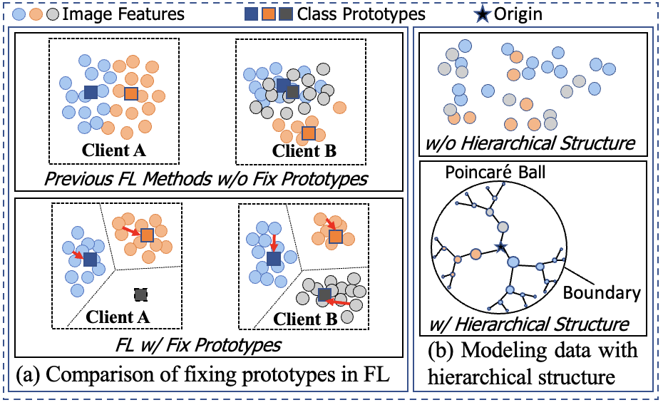
Nevertheless, most existing methods overlook three issues in FL with non-IID data. Firstly, class statistics shifting (Issue 1) happens in FL with non-IID data. Clients have different class statistics information of local data distributions, i.e., the class prototypes, which will shift and bring trivial solutions in FL without fixing. As Fig. 1(a) shows, ignoring fixing class prototypes brings two inevitable limits. Client A fails to recognize the missing class, i.e., data corresponding to some class is missing, while client B causes the class overlapping, i.e., gathering the prototypes of blue and gray classes too tight to discriminate their image features. Though FedBABU Oh et al. and SphereFed Dong et al. (2022) contribute to addressing this issue, they suffer from the dimension dilemma problem, i.e., they either lack scalability in low-dimensional space, or generate sparse representation in high-dimensional space. Secondly, current work only captures the semantic information of non-IID data, having the insufficient hierarchical information utilization issue (Issue 2). As depicted in Fig. 1(b), it is hard to gather the data samples of the same class together without hierarchical information. Hierarchical information can be helpful to group data samples and generate fine-grained representations, which can further bring prediction gains. To take this advantage, hyperbolic models are used for continuously capturing the hierarchical structure of data in the low-dimensional space Liu et al. (2020); Linial et al. (1995), whose effectiveness is proved in computer vision Khrulkov et al. (2020), recommender systems Tan et al. (2022b), and natural language processing Chen et al. (2022b). However, how to integrate existing FL methods with the hierarchical information in hyperbolic space remains unknown. Lastly, the inconsistency in aggregating clients (Issue 3) deteriorates the performance of current FL methods as well. In practice, clients usually have statistically heterogeneous data. Existing aggregation methods, e.g., weighted average with data amounts, result in the aggregated global model deviating from the optimal global model.

In this work, we propose HyperFed which contains three modules to address the above issues, respectively. To solve Issue 1 and avoid dimension dilemma, HyperFed contains hyperbolic prototype Tammes initialization (HPTI) module in server. The server first uses Tammes prototype initialization (TPI) to construct uniformly distributed class prototypes for the whole class set in hyperbolic space. Then the server fixes the position of class prototypes, and shares class prototypes to initialize the hyperbolic predictors of clients. In this way, HyperFed not only guides the consistent and separated criteria, but also introduces the statistics of missing class, both of which encourage discriminative and fine-grained feature representation for non-IID data. To avoid Issue 2, with the supervision of hyperbolic prototypes, hyperbolic prototype learning (HPL) module in each client pulls the data sample close to its ground truth class prototype, and pushes other data samples away. Thus HyperFed enjoys the benefits of predicting with hierarchical information. To tackle Issue 3, HyperFed has a consistent aggregation (CA) module that resolves the inconsistent deviations from clients to server by solving a multi-objective optimization with Pareto constraints. Hence HyperFed obtains consistent updating direction among clients, without the need of cumbersome grid search for aggregating clients.

In summary, we are the first, as far as we know, to explore hyperbolic prototypes in FL with non-IID Data. We contribute in: (1) We adopt uniformly distributed and fixed class prototypes in hyperbolic space to alleviate the impact of statistics shifting. (2) We sufficiently leverage hyperbolic representation space to capture hierarchical information for FL. (3) We optimize the aggregation of different client model to a Pareto stationary point, minimizing the impact of inconsistent clients deviations. (4) Extensive experiments on four benchmark datasets prove the effectiveness of HyperFed.

2 Related Work

2.1 Federated Learning for Non-IID Data

In terms of the goal of optimization, there are mainly three categories of common FL work that tackles non-IID data: (1) Global performance, which modifies the local objectives with a regularization term to obtain a well-performed global model Li et al. (2020). FedProx Li et al. (2020) proposes an additional proximal term to local objective, which penalizes the updated local model that is far away from the global model. FedDYN Acar et al. (2020) and MOON Li et al. (2021a) regularize the model change with both historical global and local models simultaneously. (2) Local performance, which trains a personalized model for individual clients to enhance the performance of local models T Dinh et al. (2020); and (3) Global and local performance, which empirically decomposes the network in FL into the body for universal representation, and the head for personalized classification. Fed-RoD Chen and Chao (2021) consists of two classifiers to maintain the local and global performance, respectively. However, no above work takes action to avoid class shifting. Few work fixes the classifier to fill this gap, e.g., FedBABU Oh et al. and SphereFed Dong et al. (2022). FedBABU randomly initializes and fixes the classifier during training FL, which cannot guarantee the separation of different classes is distinguishable enough. SphereFed considers fixing the classifier in hyperspherical space. But SphereFed either lacks scalability in low-dimensional space, or generates sparse representation in high-dimensional space. VFGNN Chen et al. (2022a) utilizes graph sturcture in vertical FL rather than horizontal FL. Moreover, few existing work considers utilizing hierarchical structure and consistent aggregation, which degrades FL with non-IID data.

2.2 Hyperbolic Representation Learning

Hyperbolic geometry is a non-Euclidean geometry, which can be constructed by various isomorphic models, e.g., Poincaré model Nickel and Kiela (2017). Hyperbolic modeling has been leveraged in various deep networks, such as fully-connected layers Shimizu et al. (2020), convolutional layers Shimizu et al. (2020), recurrent layers Ganea et al. (2018), classification layers Cho et al. (2019); Weber et al. (2020), graph neural networks Liu et al. (2019); Tan et al. (2022a) and Transformer Ermolov et al. (2022). However, the existing work overlooks taking the advantage of hyperbolic learning in FL. Shen et al. (2021); Mettes et al. (2019); Ghadimi Atigh et al. (2021) treat additional prior using orthogonal basis or the prior knowledge embeddings as hyperbolic prototypes, which are positioned as distant as possible from the origin, to avoid frequently updating in prototype learning. These motivate us to utilize hyperbolic prototypes in HyperFed. On the contrary, we contract the class prototypes away from the bound of the Poincaré ball model, aiming to obtain more general class semantic information.

3 Preliminary: Poincaré Ball Model

Poincaré ball model is one of the common models in hyperbolic space, which is a type of Riemannian manifold $\mathcal{M}$ with constant negative curvature. In this work, $||\bm{x}||_{2}=\sqrt{\Sigma_{i=1}^{n}x_{i}^{2}}$ is a Euclidean norm. The Poincaré is an open ball model in $n$-dimensional hyperbolic space defined as $(\mathbb{P}^{n},g^{\mathbb{P}})$, where $\mathbb{P}^{n}=\{\bm{x}\in\mathbb{R}^{n}:||\bm{x}||_{2}<1\}$ and $g^{\mathbb{P}}$ is the Riemannian metric of a Poincaré ball. $g^{\mathbb{P}}$ is conformal to the metric of Euclidean space $g^{\mathbb{E}}$, i.e., $g^{\mathbb{P}}_{\bm{x}}=\lambda_{\bm{x}}^{2}g^{\mathbb{E}},$ where $\lambda_{\bm{x}}=\frac{2}{1-||\bm{x}||_{2}^{2}}$ is the conformal factor. Given two points in the Poincaré ball model, i.e., $\bm{x}_{1},\bm{x}_{2}\in\mathbb{P}^{n}$, the Möbious addition is defined as:

$$\bm{x}_{1}\oplus\bm{x}_{2}=\frac{(1+2\langle\bm{x}_{1},\bm{x}_{2}\rangle+||\bm{x}_{2}||_{2}^{2})\bm{x}_{1}+(1-||\bm{x}_{1}||_{2})\bm{x}_{2}^{2}}{1+2\langle\bm{x}_{1},\bm{x}_{2}\rangle+||\bm{x}_{1}||_{2}^{2}||\bm{x}_{2}||_{2}^{2}}$$

We can define the geodesic, i.e., the shortest distance between these two points in the Poincaré ball as below:

$$d(\bm{x}_{1},\bm{x}_{2})=\operatorname{arcosh}(1+\frac{2||\bm{x}_{1}-\bm{x}_{2}||_{2}^{2}}{(1-||\bm{x}_{1}||_{2}^{2})(1-||\bm{x}_{2}||_{2}^{2})}).$$ (1)

For a point $\bm{x}$ in a manifold $\mathcal{M}$, the tangent space $T_{\bm{x}}\mathcal{M}$ is a vector space comprising all directions that are tangent to $\mathcal{M}$ at $\bm{x}$. Exponential map $\exp_{\bm{x}}:T_{\bm{x}}\mathcal{M}\rightarrow\mathcal{M}$ is a transformation that projects any point $\bm{u}$ from the Euclidean tangent space to the Poincaré ball referred by point $\bm{x}$, defined as:

$$\exp_{\bm{x}}(\bm{u})=\bm{x}\oplus\left(\tanh\left(\frac{\lambda_{\bm{x}}\|\bm{u}\|_{2}}{2}\right)\frac{\bm{u}}{\|\bm{u}\|_{2}}\right).$$ (2)

The reverse of $\exp_{\bm{x}}$ is logarithmic map, i.e., $\log_{\bm{x}}:\mathcal{M}\rightarrow T_{\mathbf{x}}\mathcal{M}$, which projects hyperbolic vector back to Euclidean space.

4 Method

4.1 Problem Statement

In FL with non-IID setting, we assume there are $K$ clients, containing their own models and local datasets, and a central server with global model aggregated from clients. Suppose a dataset $\mathcal{D}$ has $C$ classes indexed by $[C]$, where $[C]$ means the full set of labels in $\mathcal{D}$. Each client $k$ has access to its private local dataset $\mathcal{D}_{k}=\{\bm{x}_{k,i},y_{k,i}\}_{i=1}^{N_{k}}$, containing $N_{k}$ instances sampled from distinct distributions. Therefore, we get $\mathcal{D}=\cup_{k\in[K]}\mathcal{D}_{k}$, where the data distributions of different $\mathcal{D}_{k}$ are different. The overall objective in FL with non-IID setting is defined as below:

$$\small{\operatorname{min}}\mathcal{L}(\bm{\theta}_{1},\dots,\bm{\theta}_{K};\bm{p})=\Sigma_{k=1}^{K}p_{k}\mathbb{E}_{(\bm{x},{y})\sim D_{k}}[\mathcal{L}_{k}(\bm{\theta}_{k};(\bm{x},{y})],$$ (3)

where $\mathcal{L}_{k}(\cdot)$ is the model loss at client $k$, and $p_{k}$ indicates its weight ratio for aggregating.

Figure 2: Framework of HyperFed. We take the modeling of HyperFed with 2-dimensional Poincaré ball predictor on Cifar10 as an example.

4.2 Framework Overview

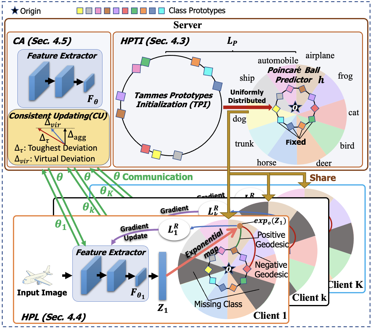
To explain how HyperFed solve the problem in FL with non-IID data, i.e., Eq. (3), we introduce the framework overview of HyperFed. In Fig. 2, there are a server and K clients. Each client or server, similarly consists of a feature extractor, an exponential map, and a Poincaré ball predictor. The feature extractor $\mathcal{F}(\cdot):\mathcal{X}\rightarrow\mathbb{R}^{d}$ maps an input data $\bm{x}$ into a $n$-dimensional vector $\bm{z}=\mathcal{F}(\bm{x})$ as feature representation. Then we get $\operatorname{exp}_{\bm{o}}(\bm{z})$ by leveraging exponential map on the feature representation $\bm{z}$ to the Poincaré ball space referred by the origin $\bm{o}$. Finally, the Poincaré ball predictor $h(\cdot):\mathbb{R}^{d}\rightarrow\mathcal{Y}$ decides class label for input data based on the representation $\operatorname{exp}_{\bm{o}}(\bm{z})$ in Poincaré ball. All Poincaré ball predictors of server and clients are fixed and shared.

As Fig. 2 shows, there are mainly three steps in HyperFed. (1) The server in HyperFed leverages hyperbolic prototype Tammes initialization (HPTI) module to construct a full set of uniformly-distributed class prototypes for the Poincaré ball predictor by Tammes prototype initialization (TPI), contracts class prototypes close to origin, and shares Poincaré ball predictor with fixed class prototypes to all of the clients. (2) Each client models local data distribution independently with the hyperbolic prototype learning (HPL) module, then sends the parameters of the local model to the server for aggregation. (3) Consistent aggregation (CA) module in the server updates the global model parameters using consistent updating (CU) to mitigate the inconsistent deviations from clients to server. After that, the server sends the new global model parameters back to clients. This communication between server and clients, i.e., steps 2-3, iterates until the performance converges.

4.3 Hyperbolic Prototype Tammes Initialization

Motivation.

In this section, we devise HPTI module in server to resolve two limits brought from the class statistics shifting, i.e., missing class and class overlapping, as described in Fig. 1(a). To bypass the dilemma of choosing a dimension, HPTI explores the class statistics in the hyperbolic space, which is scalable and effective in modeling data with low-dimensional space. Firstly, HPTI uses Tammes prototype initialization (TPI) to construct uniformly distributed and distinguishable class prototypes for the entire class set. Then HPTI fixes the position of the class prototypes on the Poincaré ball predictor. Lastly, HPTI sends the Poincaré ball predictor with fixed hyperbolic class prototypes, including the missing classes, to clients. We describe them in detail below.

HPTI first constructs uniformly distributed hyperbolic prototypes with TPI, which is available in data without prior semantic information and efficient in computation. Most work relies on prior semantic knowledge about classes to discover the positions and representations of class prototypes. However, not all datasets contain prior semantic knowledge. Motivated by Ghadimi Atigh et al. (2021), we randomly sample points on the boundary of Poincaré ball for assigning class prototypes, and optimize these points to be uniformly distributed in a ball-shaped space. In this way, we incorporate the prior with large margin separation for Poincaré ball predictor. To be specific, searching for uniformly distributed class prototypes can be formulated as a Tammes problem Tammes (1930), i.e., arranging a set of points on a unit sphere that maximizes the minimum distance between any two points. TPI optimizes this Tammes problem to obtain the class prototypes for all $C$ classes in a dataset, i.e., $\bm{W}^{*}\in\mathbb{R}^{C\times n}$ with $n$ denoting the dimension of prototype:

$$\small\begin{gathered}\bm{W}^{*}=\underset{\bm{W}\in\mathbb{P}^{n}}{\operatorname{argmin}}\left(\max_{(i,j,i\neq j)\in[C]}\bm{w}_{i}{\bm{w}_{j}}^{\top}\right),\\ \text{ s.t. }\forall i\in[C]\quad\left\|\bm{w}_{i}\right\|_{2}=1,\end{gathered}$$ (4)

where $\bm{w}_{i}$ ($\bm{w}_{j}$) is the $i-$th ($j-$th) row of $\bm{W}$ representing as the $i-$th ($j-$th) class prototype. We choose cosine similarity to measure this distance, because Poincaré ball model space is conformal to the Euclidean space Ganea et al. (2018).

Optimizing Eq. (4) requires computing pairwise similarity of class prototypes iteratively, which is inefficient. To mitigate it, we utilize the similarity of Poinecaré ball and hyper-sphere to follow Mettes et al. (2019), and minimize the largest cosine similarity for each prototype in the form of matrix, thus accelerating the optimization:

$$\small\begin{gathered}\mathbf{L}_{P}=\frac{1}{C}\Sigma_{i=1}^{C}\max_{j\in[C]}\mathbf{M}_{ij},\mathbf{M}=\bm{W}\bm{W}^{T}-2\mathbf{I},\\ \text{ s.t. }\forall i\in[C]\quad\left\|\bm{w}_{i}\right\|_{2}=1.\end{gathered}$$ (5)

Next, we find the position to fix the hyperbolic class prototypes. As Fig. 1(b) shows, in Poincaré ball model, the closer the distance from the referred origin to the node, the more general the semantic information of node represents Liu et al. (2020). But the uniformly distributed class prototypes are initially positioned on the boundary of the Poincaré ball, which is against the distribution of hierarchical structure in Poincaré ball. In order to enjoy the benefits of uniformity and generality simultaneously, we contract the class prototypes along with the radius to the origin $\bm{o}$ by a slope degree $s$, i.e., $\bm{W}_{\mathbb{P}}=s\bm{W}^{*}\in\mathbb{R}^{C\times n}$. Lastly, HPTI shares and fixes the Poincaré ball model to clients, which encourages local clients to model local data sufficiently with the supervision of consistent and separated hyperbolic prototypes.

4.4 Hyperbolic Prototype Learning

Motivation.

In this part, we provide the details of HPL, which utilizes the hierarchical information inherent in data to obtain fine-grained and gathered data representations. To utilize the hierarchical information of data, HPL uses Poincaré ball model for the benefits of continuous optimization and effective representation in low-dimensional space. To start with, HPL extracts the feature for data samples and applies an exponential map referred by the origin shared with class prototypes. According to the supervision of shared class prototypes in hyperbolic space, HPL next represents the data features of the same class according to hyperbolic triplet loss.

In the following, we present how to model the hyperbolic representations of data samples for each client $k$ locally. Specifically, we expect to learn a projection of local data $\mathcal{D}_{k}$ to the local Poincaré ball model, i.e., $\mathbb{P}^{n}_{k}$, in which we compute the similarity between data samples and class prototypes for each client. As introduced in Fig. 2, we take a feature extractor $\mathcal{F}_{\bm{\theta}_{k}}(\cdot)$ in Euclidean space to obtain the feature representations of local data samples, i.e., $\bm{z}=\mathcal{F}_{\bm{\theta}_{k}}(\bm{x})$ for an instance pair $(\bm{x},y)$ in $\mathcal{D}_{k}$. Referred by origin $\bm{o}$, we apply an exponential map from tangent space $\mathcal{T}_{\bm{o}}\mathcal{M}$ to the Poincaré ball model $\mathbb{P}^{n}_{k}$ shared with class prototypes. Hence, the representation of data samples in Poincaré ball model $\mathbb{P}^{n}_{k}$ can be:

$$\exp_{\bm{0}}(\bm{z})=\tanh(||\bm{z}||_{2})\frac{\bm{z}}{||\bm{z}||_{2}}.$$ (6)

As mentioned ahead, we seek to construct the hierarchical structure between the feature representations of data samples and their corresponding class prototypes. Triplet loss Movshovitz-Attias et al. (2017); Liu et al. (2021, 2023) optimizes the distances among a set of triplets, denoted as {anchor point, positive point, negative point}, by creating a fixed margin, i.e., $m$, between the anchor-positive points difference and the anchor-negative points difference. Motivated by this, we choose each data sample representation in the Poincaré ball model as anchor point, the ground truth class prototype as positive point, and the remaining prototypes of the full class set as negative points. In this way, each client incorporates the prototypes of its missing class to feature representation, by randomly sampling negative points. We define hyperbolic triplet loss for client $k$ as below:

$$\small\mathbf{L}_{k}^{R}=\max(d(\exp_{\bm{0}}(\bm{z}),\bm{w}_{y})-d(\exp_{\bm{0}}(\bm{z}),\bm{w}_{y^{\prime}})+m,0),$$ (7)

where $\bm{z}=\mathcal{F}_{\bm{\theta}_{k}}(\bm{x})$, $\bm{w}_{y^{\prime}}$ is randomly sampled negative class prototype, $d(\cdot,\cdot)$ is the geodesic distance defined in Eq. (1), and margin $m$ is a hyper-parameter. We obtain fine-grained representation with sufficient hierarchical information, by simultaneously minimizing the positive geodesic, e.g., the green curve in Fig. 2, and maximizing the negative geodesic, e.g., the red curve in Fig. 2. In this way, HyperFed utilizes the data hierarchical information to enhance the prediction.

Algorithm 1 Training procedure of HyperFed

Input: Batch size $B$, communication rounds $T$, number of clients $K$, local steps $E$, dataset $\mathcal{D}=\cup_{k\in[K]}\mathcal{D}_{k}$
Output: hyperbolic class prototypes $\bm{W}_{\mathbb{P}}$, model parameters, i.e., $\bm{\theta}^{T}\text{and}\{\bm{\theta}_{k}^{T}\}$

1:  Server executes():

2:  Initialize $\bm{\theta}^{0}$ with random distribution and $\bm{W}_{\mathbb{P}}$ by HPTI

3:  for $t=0,1,...,T-1$ do

4:     for $k=1,2,...,K$ in parallel do

5:        Send $\{\bm{\theta}^{t},\bm{W}_{\mathbb{P}}\}$ to client $k$ if $t=0$ else $\bm{\theta}^{t}$

6:        $\bm{\theta}_{k}^{t+1}\leftarrow$ HPL: Client executes($k$, $\bm{\theta}^{t}$)

7:     end for

8:     CA: optimize Eq. (10) with CU and update parameters of $\bm{\theta}^{t+1}$ by Eq. (8)

9:  end for

10:  return $\bm{\theta}^{T},\bm{W}_{\mathbb{P}},\{\bm{\theta}_{k}^{T}\}$

11:  HPL: Client executes($k$, $\bm{\theta}^{t}$):

12:  Assign global model to the local model $\bm{\theta}_{k}^{t}\leftarrow\bm{\theta}^{t}$

13:  for each local epoch $e=1,2,...,E$ do

14:     for batch of samples $(\bm{x}_{k,1:B},\bm{y}_{k,1:B})\in\mathcal{D}_{k}$ do

15:        Feature extraction $\bm{z}_{k,1:B}\leftarrow\mathcal{F}_{\bm{\theta}_{k}^{e}}(\bm{x}_{k,1:B})$

16:        Project $\bm{z}_{k,1:B}$ to Poincaré ball by Eq. (6)

17:        Compute loss $\mathbf{L}_{k}^{R}$ by Eq. (7)

18:        Update parameters of $\bm{\theta}_{k}^{e}$ by RSGD

19:     end for

20:  end for

21:  return $\bm{\theta}_{k}^{E}$ to server

4.5 Consistent Aggregation

Motivation.

Finally, we introduce CA which mitigates the inconsistent deviations from clients to server caused by the statistically heterogeneous data distributions. In FL aggregation, CA first formulates the aggregation of local feature extractors in HyperFed  as a multi-objective optimization. Then CA applies consistent updating (CU) to pick the toughest client, i.e., the client with the most divergent deviation, and alleviate the inconsistency between the toughest client and the remaining clients. Lastly, CU iteratively optimizes this multi-objective optimization to yield a Pareto optimal solution and obtain the weight ratio of different client models.

We formulate the aggregation as a multi-objective optimization in the following. Specifically, we first compute the different deviations from clients to server as multiple objectives, then the goal of alleviating the inconsistency of these deviations can be achieved by multiple-objective optimization. We obtain the combination of local parameters in server:

$$\bm{\theta}^{t+1}=\bm{\theta}^{t}+\Sigma_{k=1}^{K}p_{k}\left(\bm{\theta}_{k}^{t+1}-\bm{\theta}^{t}\right),$$ (8)

where $\bm{\theta}^{t}$ is the global model and $\bm{\theta}_{k}^{t}$ is the local model of the client $k$ at $t-$th communication. Next, we denote global and client deviations, i.e., $\Delta_{\bm{\theta}}^{t+1}=\bm{\theta}^{t+1}-\bm{\theta}^{t}$ and $\Delta_{\bm{\theta}_{k}}^{t+1}=\bm{\theta}_{k}^{t+1}-\bm{\theta}^{t}$, respectively, and rewrite Eq. (8) as:

$$\Delta_{\bm{\theta}}^{t+1}=\Sigma_{k=1}^{K}p_{k}\Delta_{\bm{\theta}_{k}}^{t+1}.$$ (9)

Then CA solves this multiple-objective optimization to Pareto stationary point, i.e., minimizing the minimum possible convex combination of inconsistent deviations:

$$\min\frac{1}{2}\left\|\Sigma_{k=1}^{K}p_{k}\Delta_{\bm{\theta}_{k}}^{t+1}\right\|^{2}_{2}\text{, s.t. }\Sigma_{k=1}^{K}p_{k}=1\text{, and }\forall k,p_{k}\geq 0.$$ (10)

Next, we introduce CU which derives from Multiple Gradient Descent Algorithm (MGDA) Désidéri (2012); Sener and Koltun (2018) to solve this optimization. The optimization problem defined in Eq. (10) is equivalent to finding a minimum-norm point in the convex hull of the set of input points, i.e., a convex quadratic problem with linear constraints. CU iteratively optimizes Eq. (10) by linear search, which can be solved analytically Jaggi (2013). In detail, we find the toughest client, treat the combination of the remaining clients as a virtual client, and analyze the solution according to the directions of the toughest client and the virtual client. Firstly, we initialize $\bm{p}_{0}$ with the weight of data samples, i.e., $p_{k}=\nicefrac{{N_{k}}}{{\Sigma_{k=1}^{K}N_{k}}}$, and precompute the consistency of deviations $\bm{V},s.t.\bm{V}_{k,k^{\prime}}={\Delta_{\bm{\theta}_{k}}}^{\top}{\Delta_{\bm{\theta}_{k^{\prime}}}}$. Then we find the toughest client by $\tau=\operatorname{arg}\operatorname{min}_{k^{\prime}}\Sigma_{k=1}^{K}p_{k}\bm{V}_{k^{\prime},k}$ with deviation $\Delta_{\tau}$, and remain the combination of others with historical weights to be a virtual client, i.e., $\Delta_{\text{vir}}=\Sigma_{k=1,k\neq\tau}^{K}p_{k}\Delta_{\bm{\theta}_{k}}$. Thus we simplify Eq. (10), i.e., $\operatorname{min}_{p_{\tau}\in[0,1]}\frac{1}{2}\|p_{\tau}\Delta_{{\tau}}+(1-p_{\tau})\Delta_{{\text{vir}}}\|^{2}_{2}$. According to the directions of $\Delta_{\tau}$ and $\Delta_{\text{vir}}$, we can obtain the analytical solution for $p_{\tau}$:

$$p_{\tau}=\operatorname{CU}^{+}\left[\nicefrac{{{(\Delta_{\text{vir}}-\Delta_{\tau})}^{\top}\Delta_{\text{vir}}}}{{\|\Delta_{\tau}-\Delta_{\text{vir}}\|^{2}_{2}}}\right],$$ (11)

where $\operatorname{CU}^{+}[\cdot]=\operatorname{max}(\operatorname{min}(\cdot,1),0)$. In Appendix C, we present the analysis of optimization for obtaining $\operatorname{CU}^{+}[\cdot]$ based on the computational geometry Sekitani and Yamamoto (1993) of minimum-norm in the convex hull. Given $p_{\tau}$, we update the weight ratio $\bm{p}=(1-p_{\tau})\bm{p}+p_{\tau}\bm{e}$, where $\bm{e}$ is the one-hot vector with 1 in the $\tau-$th position. In order to obtain the Pareto stationary point, CU iterates the process of finding the toughest client several times to obtain the best combination $\bm{p}^{*}$ that alleviates the inconsistent deviations of clients. Finally, we find the consistent optimization direction with the Pareto optimal solution $\bm{p}^{*}$ for aggregating in Eq. (8).

Given three main modules, i.e., HPTI, HPL, and CA, we illustrate the overall algorithm of modeling HyperFed in Algo. 1. Steps 1-10 are the server execution. In step2, the server initializes model parameters and HPTI in it initializes the hyperbolic class prototypes. Then for each communication round, all clients use HPL to train their local model with the shared Poincaré ball predictor in step 6. After that, in step 8, CA in server receives the model parameters of all clients, and mitigates the inconsistency of client deviations in aggregation. The details of client execution is listed in steps 11-21.

5 Experiments and Discussion

5.1 Experimental Setup

Datasets.

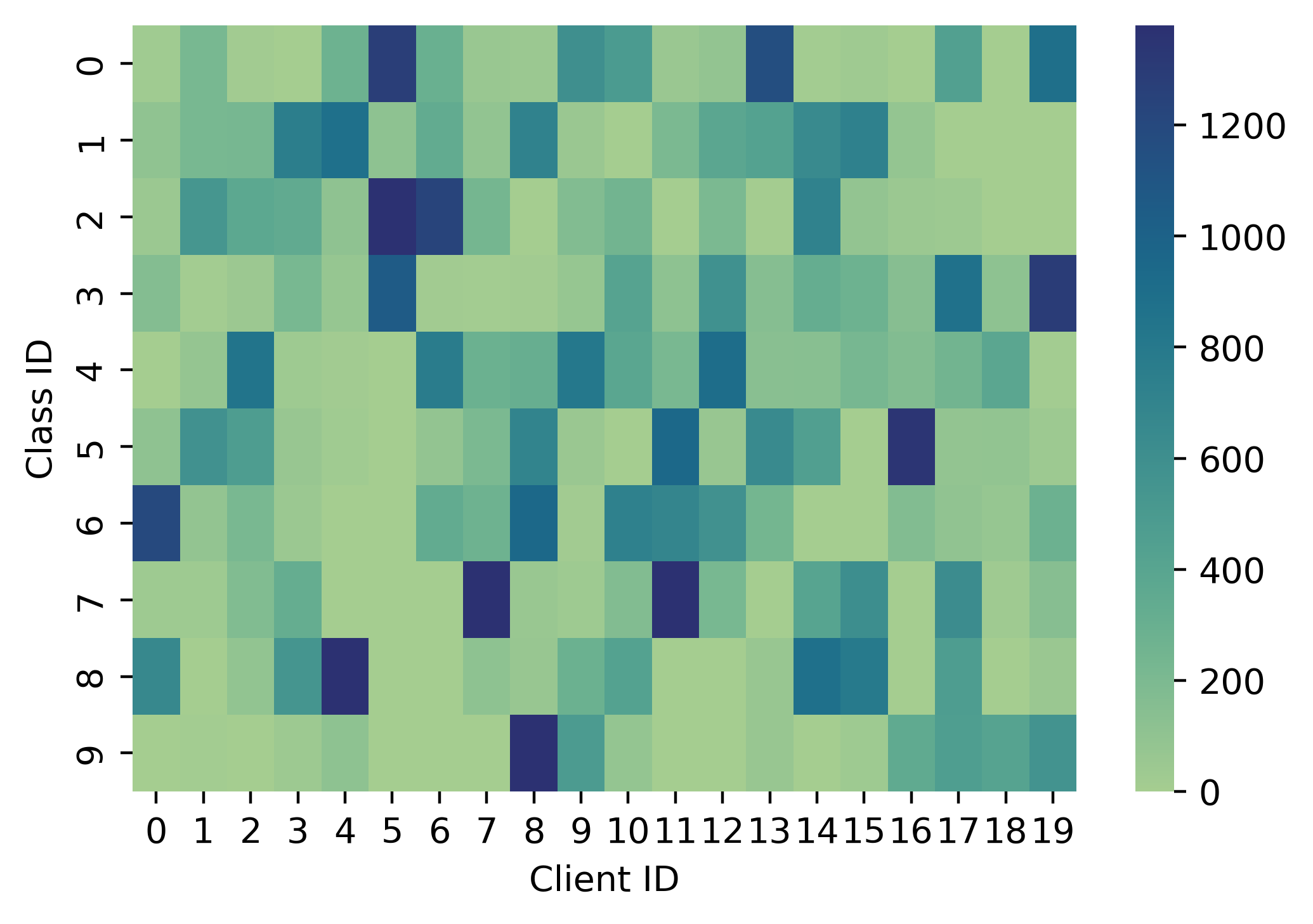
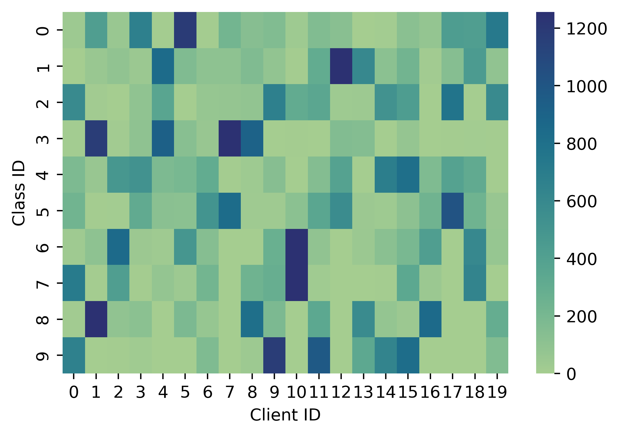
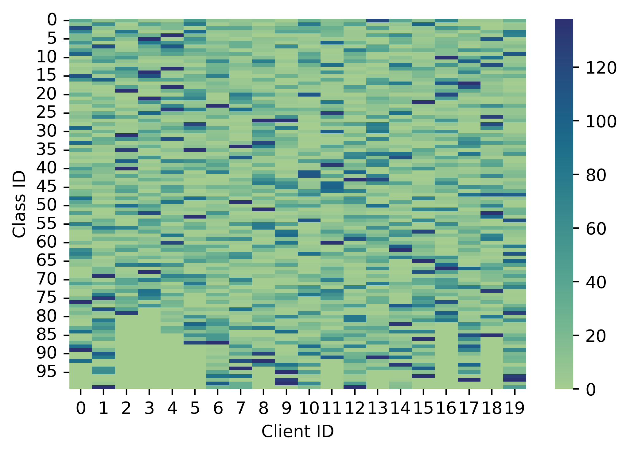
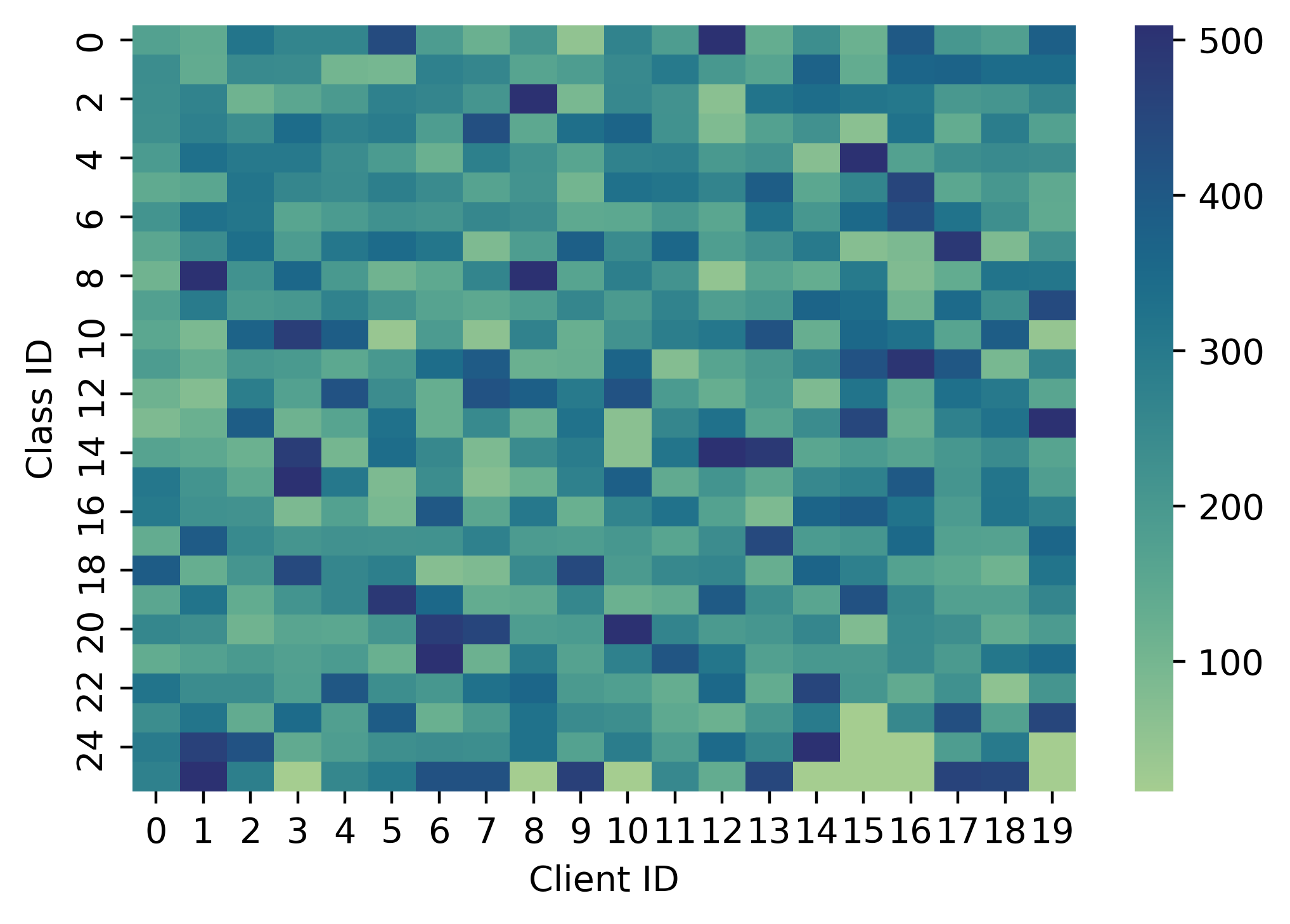
We use four public datasets in torchvision, i.e., EMNIST by Letters Cohen et al. (2017), Fashion-MNIST (FMNIST) Xiao et al. (2017), Cifar10, and Cifar100 Krizhevsky et al. (2009), which are widely-used in the recent FL work Chen and Chao (2021); Oh et al. ; Li et al. (2021a). There are two evaluation goals for FL with non-IID data, i.e., global performance (G-FL) and local personalized performance (P-FL). G-FL tests the global model aggregated in the server by evaluating the test set published in the torchvision. In P-FL, we simulate local data distribution using the train set published in torchvision to evaluate the local models. For all datasets, we simulate the non-IID data distributions following Hsu et al. (2019); Li et al. (2021a). Specifically, we sample a proportion of instances of class $j$ to client $k$ with Dirichlet distribution, i.e., $p_{j,k}\sim{Dir}_{N}(\alpha)$, where $\alpha$ denotes the non-IID degree of every class among the clients. The smaller $\alpha$ indicates the more heterogeneous data distribution. We sample 75% of local data as local training set and the remaining as local test set.

Comparison Methods.

We compare HyperFed with three categories of state-of-the-art approaches according to their optimization goals, i.e., (1) optimizing global model: FedAvg McMahan et al. (2017), FedProx Li et al. (2020), SCAFFOLD Karimireddy et al. (2019), FedDYN Acar et al. (2020), MOON Li et al. (2021a), (2) optimizing local personalized models: FedMTL Smith et al. (2017), FedPer Arivazhagan et al. (2019), pFedMe T Dinh et al. (2020), Ditto Li et al. (2021b), APPLE Luo and Wu (2021), and (3) optimizing both global and local models: Fed-RoD Chen and Chao (2021), FedBABU Oh et al. , and SphereFed Dong et al. (2022).

Implementation Details.

We adopt ConvNet LeCun et al. (1998) as a feature extractor for EMNIST and FMNIST, while ResNet He et al. (2016) for Cifar10 and Cifar100. We set all of the datasets with batch size as 128 and embedding dimension as 20. For HyperFed, we choose RSGD Bonnabel (2013) as the optimizer, set the learning rate $lr=0.3$, the margin $m=3$, and the slope degree $s=0.9$. We conduct training for all of the methods with 5 local epochs per round until converge. We evaluate both G-FL and P-FL by top-1 accuracy. We set the non-IID degree $\alpha=\{0.1,0.5,5\}$, respectively, for evaluating the performance of different methods.

Figure 3: UMAP visualizations on FMNIST ($\alpha=0.5$).

Dataset	EMNIST			FMNIST			Cifar10			Cifar100
Method \NonIID	Dir(0.1)	Dir(0.5)	Dir(5)	Dir(0.1)	Dir(0.5)	Dir(5)	Dir(0.1)	Dir(0.5)	Dir(5)	Dir(0.1)	Dir(0.5)	Dir(5)
FedAvg	88.86	92.86	93.31	78.51	86.75	88.75	36.82	62.44	67.53	27.61	29.26	30.12
FedProx	90.75	93.27	93.65	78.49	86.57	88.68	37.95	63.48	67.23	26.91	29.77	29.98
SCAFFOLD	90.35	93.38	93.70	79.20	87.03	88.80	33.10	66.99	70.53	29.57	33.25	33.86
FedDYN	91.30	92.63	93.13	85.25	89.46	90.51	35.16	65.07	69.04	29.16	31.49	32.21
MOON	91.97	93.50	93.91	83.78	90.27	91.08	33.54	60.23	62.45	22.86	24.49	25.99
Fed-RoD	89.42	92.80	93.52	77.26	89.17	90.78	37.79	66.90	70.81	17.06	24.32	31.99
FedBABU	86.34	91.95	92.74	74.31	82.44	85.21	37.90	60.11	65.16	22.98	24.56	23.89
SphereFed	93.25	93.93	94.07	88.55	90.55	91.17	32.41	70.02	70.13	22.37	24.96	24.72
HyperFed-Geodesic	93.35	94.13	94.43	79.00	90.76	91.48	34.26	65.53	68.65	26.05	29.07	26.62
HyperFed-Shared	93.82	93.98	94.16	85.29	90.48	91.23	36.44	69.21	73.16	33.62	35.31	36.30
HyperFed-Averaged	93.65	94.29	94.45	87.91	90.98	91.69	36.69	70.12	70.81	33.39	36.33	36.93
HyperFed	94.00	94.33	94.46	89.38	91.16	91.83	38.03	71.25	75.22	33.93	38.89	37.50

Table 1: G-FL accuracy ($\%$) of the global model. We bold the best result.

Dataset	EMNIST			FMNIST			Cifar10			Cifar100
Method \NonIID	Dir(0.1)	Dir(0.5)	Dir(5)	Dir(0.1)	Dir(0.5)	Dir(5)	Dir(0.1)	Dir(0.5)	Dir(5)	Dir(0.1)	Dir(0.5)	Dir(5)
FedMTL	96.28	91.08	88.21	97.39	90.89	85.71	90.57	65.68	48.31	46.28	24.72	11.64
FedPer	97.23	94.19	92.97	96.87	90.54	87.21	91.93	75.63	67.20	49.69	32.75	23.89
pFedMe	97.23	94.03	92.62	96.03	88.57	84.95	92.45	77.64	66.09	55.20	36.34	28.19
Ditto	97.72	95.32	94.30	97.79	93.75	92.05	91.34	74.35	69.94	47.08	31.89	27.04
APPLE	97.19	94.08	92.63	96.79	90.49	86.59	89.85	67.96	56.13	42.94	24.61	20.39
Fed-RoD	97.76	95.31	93.99	97.21	93.48	91.62	91.24	72.11	71.33	35.03	27.70	32.22
FedBABU	97.36	94.17	92.81	96.64	89.59	85.57	92.04	64.05	63.46	29.30	25.05	24.01
SphereFed	93.61	94.11	94.34	88.91	90.87	91.88	91.68	78.39	72.86	40.68	32.63	34.90
HyperFed-Geodesic	97.97	95.60	94.48	97.00	93.98	91.89	91.68	72.20	69.02	29.70	27.11	27.03
HyperFed-Fixed	97.96	95.65	94.45	96.53	92.66	90.85	90.57	79.66	59.38	49.08	20.20	11.31
HyperFed-Shared	97.50	95.66	94.39	97.50	93.00	91.52	92.69	77.43	71.62	47.97	33.16	35.19
HyperFed-Averaged	97.71	95.13	94.46	97.83	93.73	91.96	92.63	70.53	69.02	53.50	36.49	35.79
HyperFed	98.76	96.11	94.53	98.13	94.19	92.08	93.49	83.17	74.94	59.85	40.94	36.80

Table 2: P-FL accuracy ($\%$) of the local model. We bold the best result.

(a) G-FL

(b) P-FL

Figure 4: Effect of local epochs $E$ on Cifar10 ($\alpha=0.5$).

(a) G-FL

(b) P-FL

Figure 5: Effect of slope degree $s$ on FMNIST $\&$ Cifar10 ($\alpha=0.5$)

(a) G-FL

(b) P-FL

Figure 6: Effect of margin $m$ on FMNIST $\&$ Cifar10 ($\alpha=0.5$).

(a) G-FL

(b) P-FL

Figure 7: Effect of clients number $K$ on FMNIST ($\alpha=0.5$).

Dataset	Goal	2	5	10	20	25	50	100
FMNIST	P-FL	88.91	93.20	93.84	93.98	93.70	93.73	93.66
($\alpha$=0.5)	G-FL	88.59	91.07	90.91	91.16	90.74	90.74	90.74
Cifar10	P-FL	72.82	80.55	82.83	83.17	82.50	83.15	82.76
($\alpha$=0.5)	G-FL	60.87	68.82	69.84	71.25	70.67	71.51	71.69

Table 3: Effect of the representation dimension in HyperFed.

5.2 Empirical Results

Performance Comparison.

We run each method 5 times and report the performance of G-FL and P-FL in Tab. 1-2 with the average value, respectively. There are mainly three observations. (1) In terms of G-FL evaluated in Tab. 1, generally speaking, the performance of G-FL is increasing along with the increase of non-IID degree $\alpha$. It states that the heterogeneity of data distribution deteriorates the performance of FL methods. FedAvg takes no measure to handle non-IID, which is worse than most methods. Similarly, FedBABU is a variant of FedAvg that fixes the randomly initialized classifier, perform inferior as well. It means that simply fixing the classifier initialized by random is not enough for FL with non-IID data. (2) In terms of P-FL evaluated in Tab. 2, the methods of the third category can achieve accuracy similar as the second category on FMNIST and EMNIST, but cannot maintain the personalization on Cifar100. This indicates that simply fixing class statistics in FL is less promising than personalization strategies on complex dataset. SphereFed is the runner-up of Cifar100 ($\alpha=5$), but it fails to perform well on more heterogeous setting, i.e., Cifar100 ($\alpha=\{0.1,0.5\}$). This phenomenon shows that HyperFed performs better for FL with non-IID data, as a FL method of the third category. (3) In terms of the performance of HyperFed, HyperFed achieves the best results in all kinds of non-IID degrees and different datasets, which verifies the efficacy of HyperFed for non-IID problems. In the results of Cifar100, HyperFed significantly outperforms all of the comparison algorithms listed both in G-FL and P-FL, in terms of at least 10.75% and 5.44%, respectively. This shows that HyperFed can capture more fine-grained representation to improve performance, especially on large and complicated datasets with low dimensional representation.

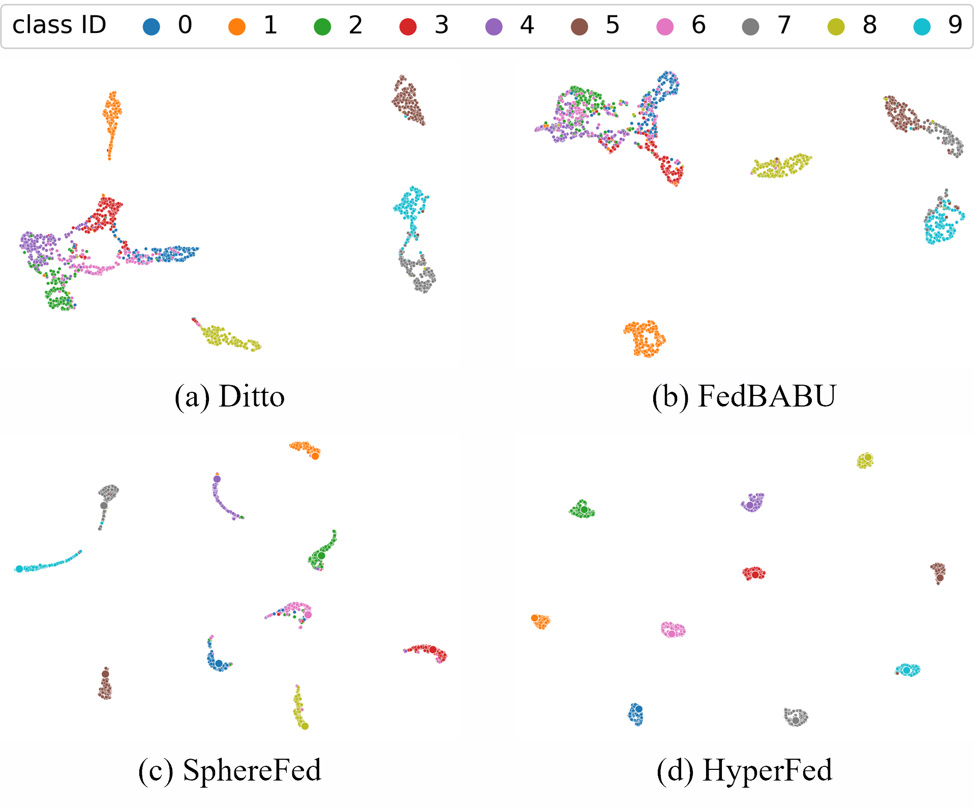
Visualization. To verify the benefits of fixing class statistics in hyperbolic space, we utilize UMAP McInnes et al. (2018) to visualize the G-FL hidden representations of the global model in HyperFed, the runner-up of G-FL,i.e., SphereFed, and P-FL, i.e., Ditto, and FedBABU on FMNIST ($\alpha=0.5$) in Fig. 3. we can find that: (1) Compared with Ditto, methods fixing the class statistics attain more gathered representations. (2) Though FedBABU fixes the classifier, the randomly initialized classifier is limited in resolving class overlapping. (3) Compared with SphereFed whose classifier is initialized with a set of orthogonal basis in hypersphere, HyperFed concentrates the hidden representation tighter due to sufficiently utilizing the hierarchical information.

Ablation Studies.

We consider four variants of HyperFed: (1) HyperFed uses geodesic as metric, i.e., HyperFed-Geodesic, (2) HyperFed uses fixed class prototypes only, i.e., HyperFed-fixed, (3) HyperFed uses shared class prototypes only, i.e., HyperFed-shared, and (4) HyperFed uses weighted average aggregation by data amounts, i.e., HyperFed-Averaged. From Tab. 1-2, we can discover that: All of the variants decrease their performance compared with HyperFed. These results identify that all of the components of HyperFed, contribute to performance enhancement.

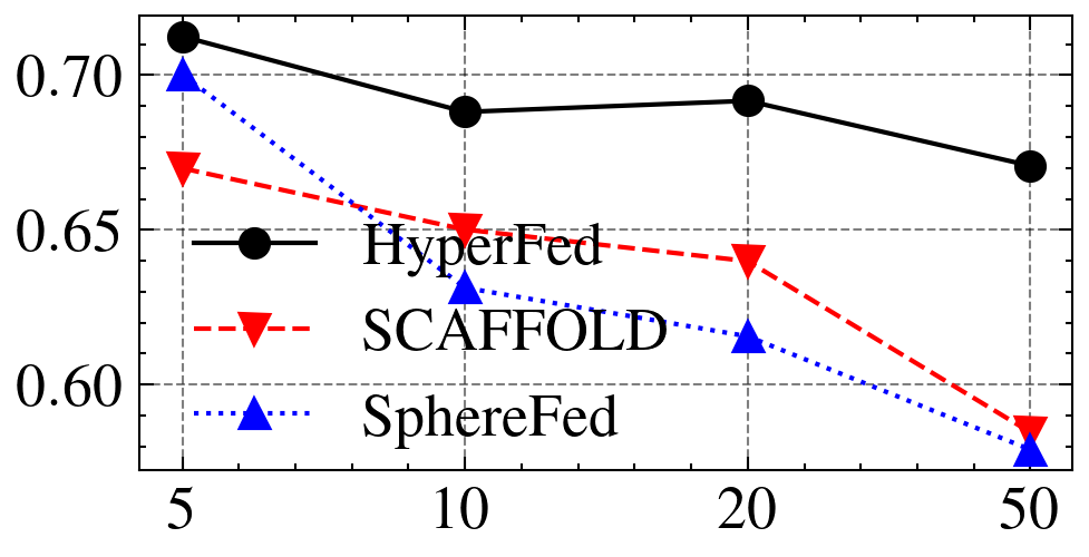
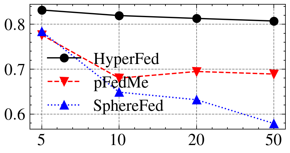
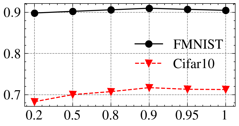
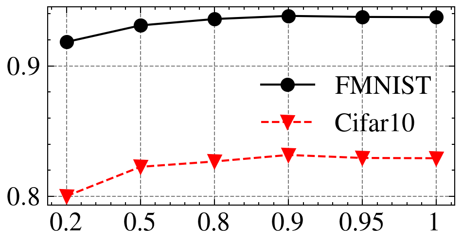
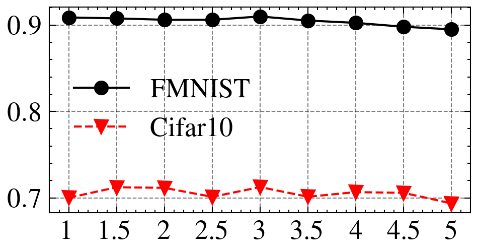
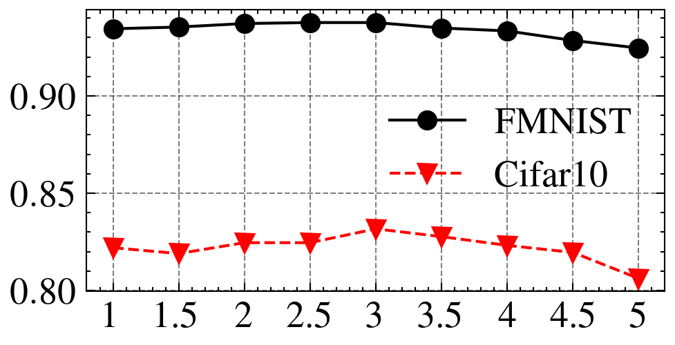
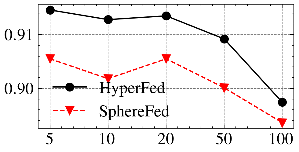
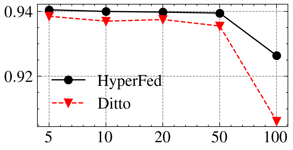
Hyper-parameters Sensitivity. To study the sensitivity of hyper-parameters, we compare the performance of FMNIST and Cifar10 by varying the local epochs $E=\{5,10,20,50\}$ in Fig. 4, slope degree $s=\{0.2,0.5,0.8,0.9,0.95,1\}$ in Fig. 5, margin $m=\{1,1.5,2,2.5,3,3.5,4,4.5,5\}$ in Fig. 6, number of clients $K=\{5,10,20,50,100\}$ in Fig. 7, and the dimension of features representation $d=\{2,5,10,20,25,50,100\}$ in Tab. 3, respectively. We can conclude that: (1) The increase of local epochs per communication round decreases the performance of FL methods. (2) HyperFed nearly converges when $s=0.9$, which indicates that positioning the class prototypes in 90% of radius achieves a balance between the best model performance and the most general class information. (3) The performance of HyperFed varying by $m$ forms a slight bell curve. (4) HyperFed outperforms the runner-up methods in all cases of different number of clients. (5) The dimension changes slightly affect the performance of HyperFed, proving that HyperFed is proficient in low-dimensional representation.

6 Conclusion

To enhance federated learning (FL) with non-IID data, we propose HyperFed which contains hyperbolic prototype Tammes initialization (HPTI) module, hyperbolic prototype learning (HPL) module, and consistent aggregation (CA) module. Firstly, HPTI constructs uniformly distributed and fixed class prototypes on server, and shares them with clients to guide consistent feature representation for local clients. secondly, HPL models client data in the hyperbolic model space with the supervision of shared class prototypes. Additionally, CA mitigates the impact of inconsistent deviations from clients to server. Extensive studies on four datasets prove the effectiveness of HyperFed.

Appendix A Datasets

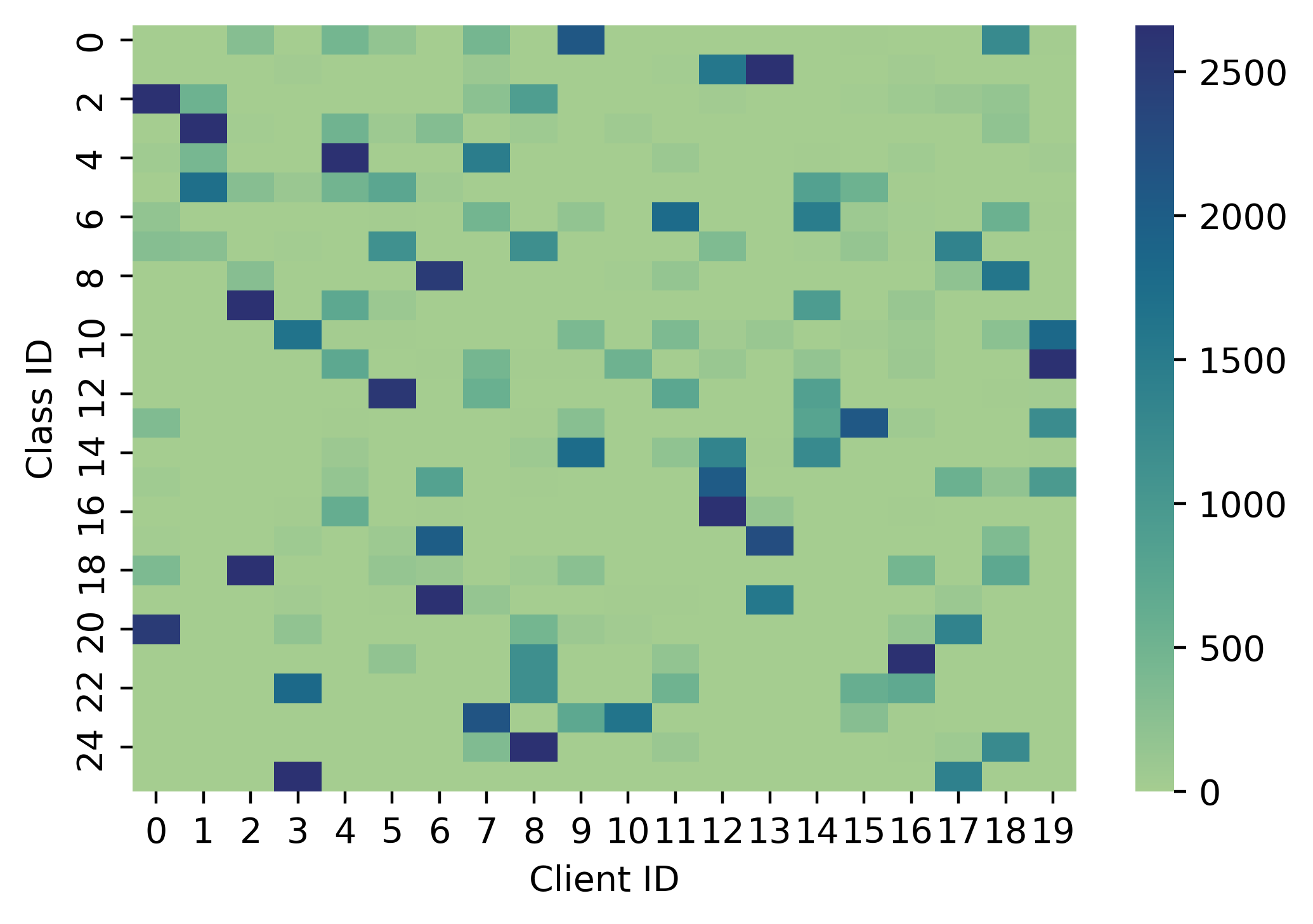
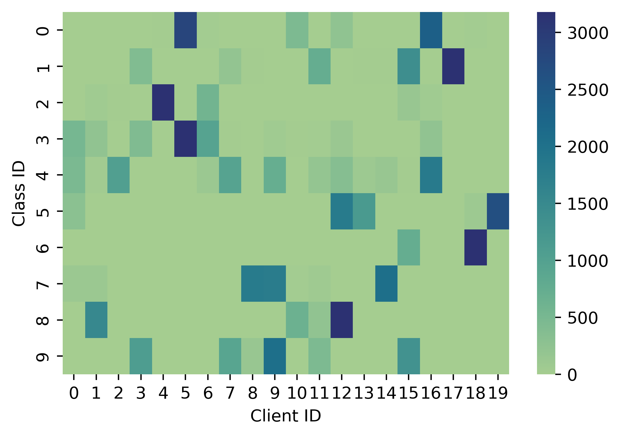
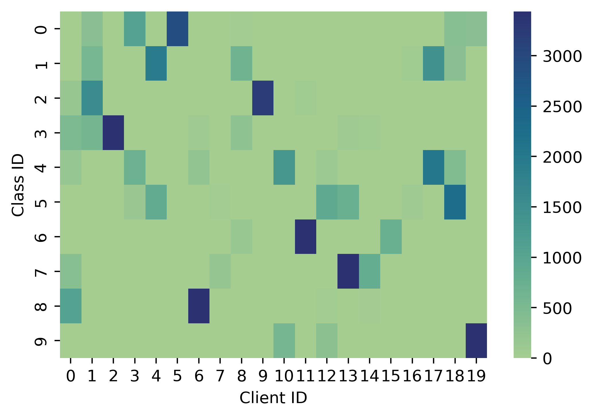
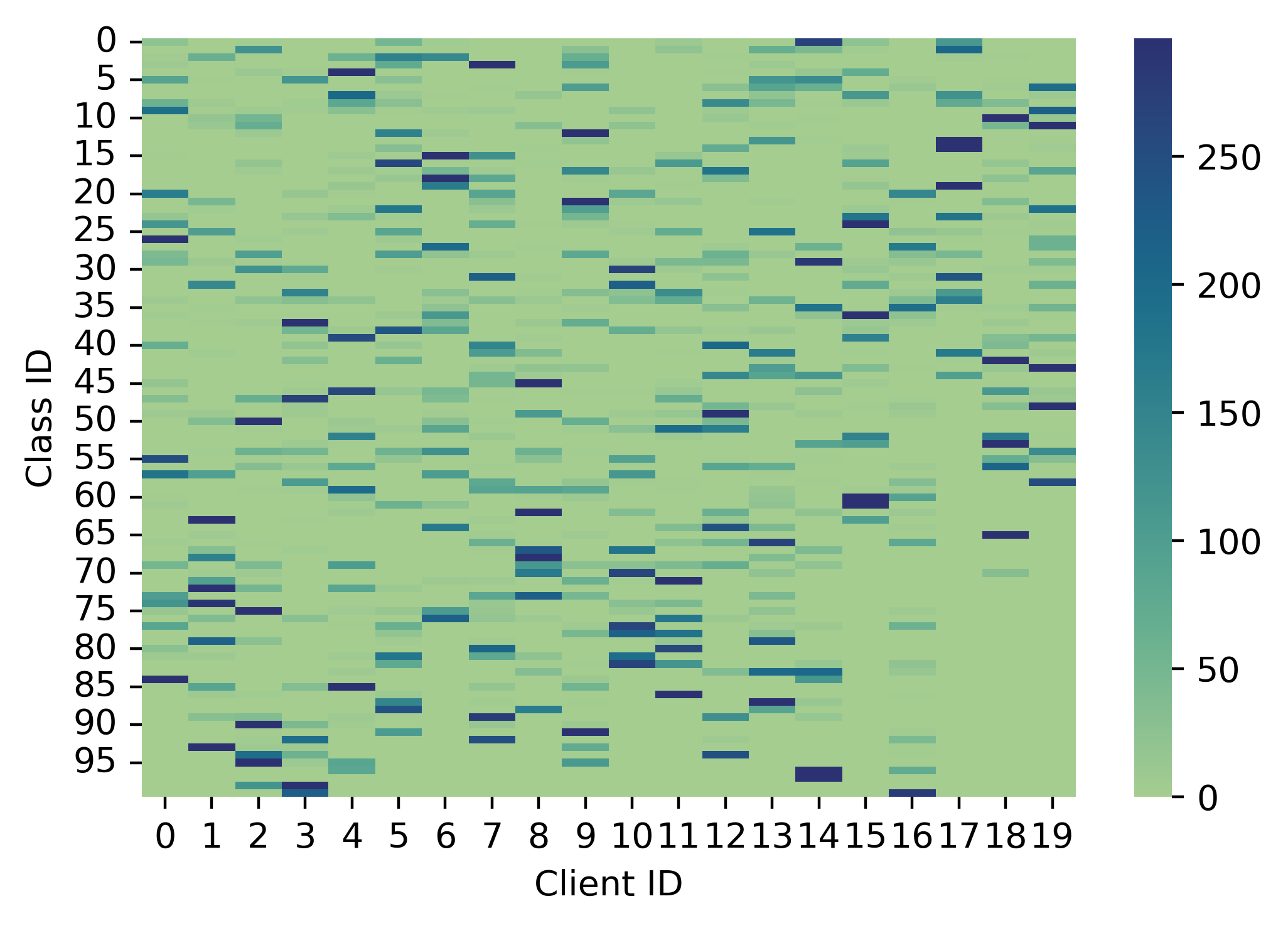
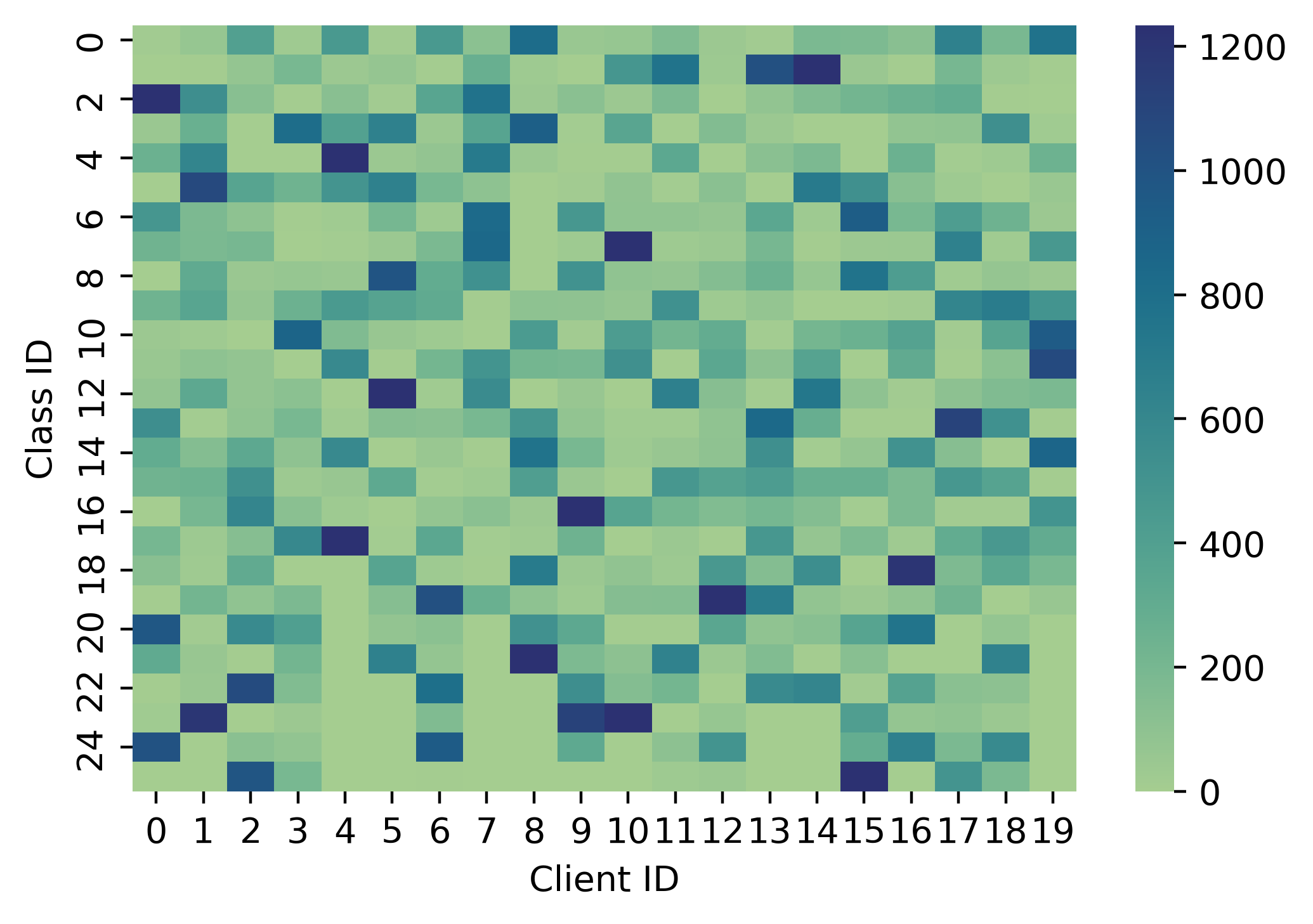
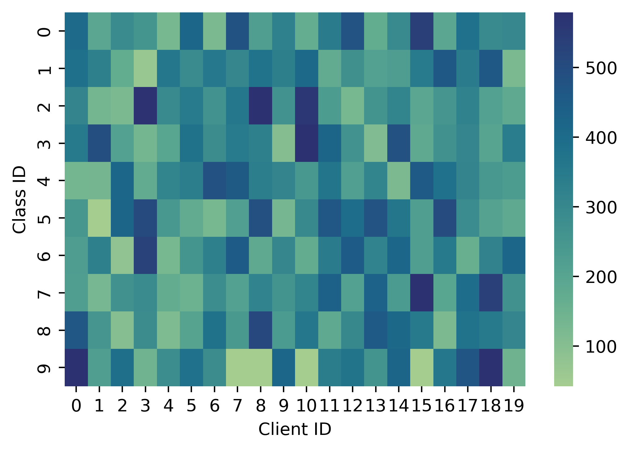
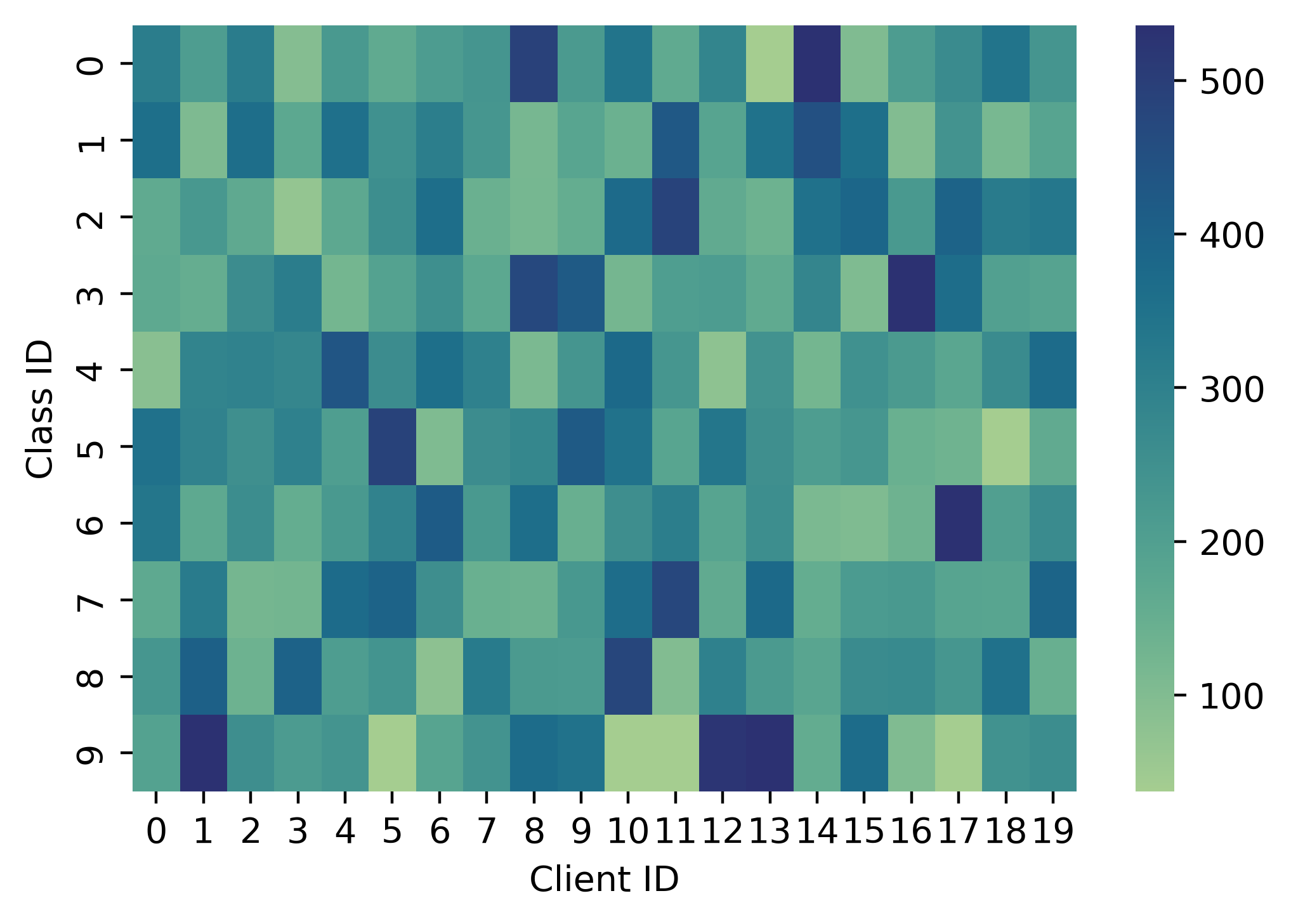
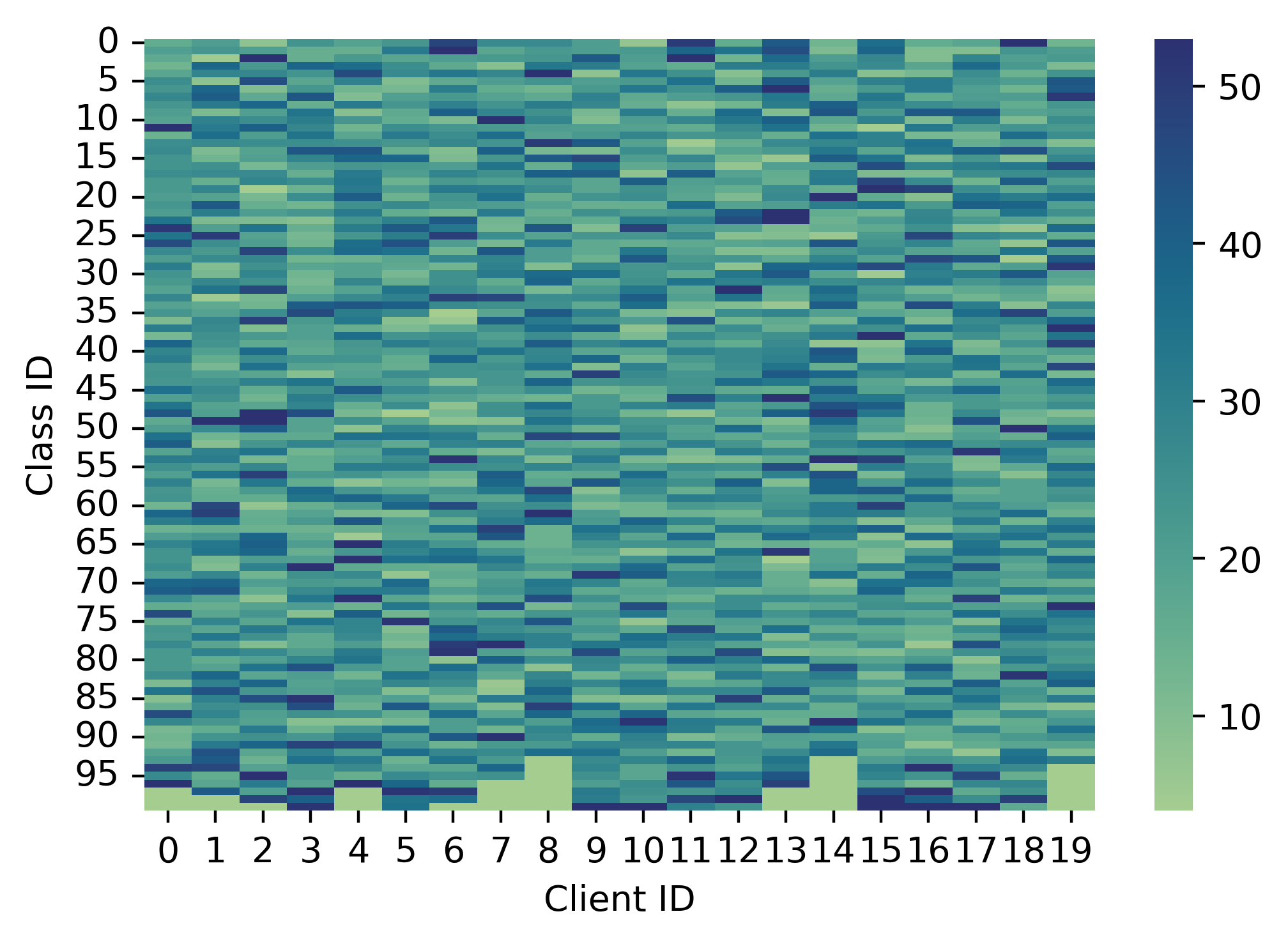
We visualize the data distributions under different degrees of non-IID, i.e., $\alpha=\{0.1,0.5,5\}$ for EMNIST, FMNIST, Cifar10, and Cifar100 in Fig. 8-Fig. 10.

(a) EMNIST $\alpha=0.1$

(b) FMNIST $\alpha=0.1$

(c) Cifar10 $\alpha=0.1$

(d) Cifar100 $\alpha=0.1$

Figure 8: Distributions of $\alpha=0.1$.

(a) EMNIST $\alpha=0.5$

(b) FMNIST $\alpha=0.5$

(c) Cifar10 $\alpha=0.5$

(d) Cifar100 $\alpha=0.1$

Figure 9: Distributions of $\alpha=0.5$.

(a) EMNIST $\alpha=5$

(b) FMNIST $\alpha=5$

(c) Cifar10 $\alpha=5$

(d) Cifar100 $\alpha=5$

Figure 10: Distributions of $\alpha=5$.

Appendix B Details of Comparison Methods

We compare HyperFed with three categories of state-of-the-art approaches according to their optimization goals, i.e., (1) optimizing global model: FedAvg McMahan et al. [2017], FedProx Li et al. [2020], SCAFFOLD Karimireddy et al. [2019], FedDYN Acar et al. [2020], MOON Li et al. [2021a], (2) optimizing local personalized models: FedMTL Smith et al. [2017], FedPer Arivazhagan et al. [2019], pFedMe T Dinh et al. [2020], Ditto Li et al. [2021b], APPLE Luo and Wu [2021], and (3) optimizing both global and local models: Fed-RoD Chen and Chao [2021], FedBABU Oh et al. , SphereFed Dong et al. [2022]. FedAvg is the first vanilla federated learning framework to collaborate among server and clients. FedProx takes a proximal term to regularize the change from global model to the local model. SCAFFOLD considers the variance of global model and local model when updating local gradients. FedDYN applies an dynamic regularizer to pull local model close to the global model, while to push local model away from historical local model. MOON introduces contrastive learning to federated learning. FedMTL is an algorithm that takes personalized learning as a multi-task learning objective. FedPer decouples the global representation and local personalized classification. pFedMe uses Moreau envelopes as clients’ regularized loss functions to decouple personalized model optimization from the global model learning. Ditto is a multi-task learning objective for federated learning that provides personalization while retaining similar efficiency. APPLE adaptively learns to personalize the client models. Fed-RoD explicitly decouples a model’s dual duties with two prediction tasks. FedBABU only updates the representation body of the model during federated training, and the head is fine-tuned for personalization during the evaluation process. SphereFed is a hyperspherical federated learning framework to address PFL problem.

We conduct all of the experiments on one NVIDIA RTX 3090 GPU with 24Gb Memory. In the first category of methods, a hyper-parameter $\mu$ is mainly set to balance the local objective and regularization term (between the global model and local model). According to the optimal results, we set $\mu=0.01,1,0.1,$ for FedProx, MOON, and FedDYN, respectively. Besides, we set $\tau=0.5$, the default temperature of MOON as specified in the original paper. For all of the second category of methods as well as the third category of methods, we follow the personalized way as their original setting. We similarly finetune HyperFed and FedBABU with additional 5 local steps in P-FL. For pFedMe, we set regularization parameter $\mu=1$ for controlling the strength of personalized model, computation complexity $k=5$, the interpolation parameter $\beta=1$ for global weights. We choose hyper-parameter controlling the interpolation between global and local model , i.e., $\lambda=1$ and local personalized iteration as 1 for Ditto. In APPLE, we take the hyper-parameter $\mu=0.001$, and the round number $L=0.2$ for loss scheduler.

Appendix C Theoretical Analysis

C.1 Convex Optimization

Figure 11: Computational geometry of the deviations of the toughest client and the virtual client.

For the simplified optimization of the convex combination between the toughest deviation and the virtual deviation:

$$\operatornamewithlimits{min}\limits_{p_{\tau}\in[0,1]}\frac{1}{2}\|p_{\tau}\Delta_{{\tau}}+(1-p_{\tau})\Delta_{{\text{vir}}}\|^{2}_{2},$$ (12)

we rewrite it as:

$$\min_{p_{\tau}\in[0,1]}J=\frac{1}{2}\left\|p_{\tau}\left(\Delta_{{\tau}}-\Delta_{{\text{vir}}}\right)+\Delta_{{\text{vir}}}\right\|_{2}^{2}.$$ (13)

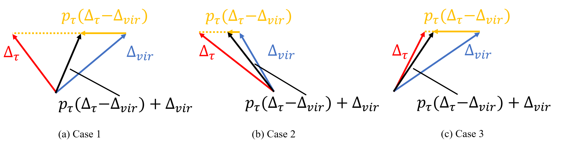
Next, we can analyze the solution according to its geometry, i.e., analyzing the directions among the toughest deviation, the virtual deviation, and their difference. As the geometry suggests in Fig. 11, the solution of finding the minimized norm is either a perpendicular vector or an edge case. Thus we obtain the three cases as bellow:

Case 1

When it has the condition as:

$$\left\{\begin{array}[]{l}\left(\Delta_{{\tau}}-\Delta_{{\text{vir}}}\right)^{\top}\cdot\Delta_{{\tau}}\ >0\\ \left(\Delta_{{\tau}}-\Delta_{{\text{vir}}}\right)^{\top}\cdot\Delta_{{\text{vir}}}<0,\end{array}\right.$$ (14)

Then we should take the differentiation $\frac{\partial J}{\partial p_{\tau}}=0$ and get:

$$\left(\Delta_{{\tau}}-\Delta_{{\text{vir}}}\right)^{\top}\left(p_{\tau}\Delta_{{\tau}}+(1-p_{\tau})\Delta_{{\text{vir}}}\right)=0.$$ (15)

Hence the solution is given:

$$\begin{gathered}p_{\tau}^{*}=\frac{\left(\Delta_{{\text{vir}}}-\Delta_{{\tau}}\right)^{\top}\cdot\Delta_{{\text{vir}}}}{\left\|\Delta_{{\tau}}-\Delta_{{\text{vir}}}\right\|_{2}^{2}}\quad\Leftrightarrow\quad\\ \Delta_{\bm{\theta}}^{t+1}=(1-p_{\tau}^{*})\Delta_{{\text{vir}}}+{p_{\tau}^{*}}\Delta_{\tau}.\end{gathered}$$ (16)

In this scenario, we find the perpendicular vector of the difference between the virtual deviation and the toughest deviation to obtain the minimum-norm.

Case 2

When it has the condition as:

$$\left(\Delta_{{\tau}}-\Delta_{{\text{vir}}}\right)^{\top}\cdot\Delta_{{\text{vir}}}\geq 0,$$ (17)

the solution

$$p_{\tau}^{*}=0\quad\Leftrightarrow\quad\Delta_{\bm{\theta}}^{t+1}=\Delta_{{\text{vir}}}.$$ (18)

In this scenario, the $\left\|\Delta_{{\text{vir}}}\right\|_{2}^{2}$ is smaller than $\left\|\Delta_{{\tau}}\right\|_{2}^{2}$. The smaller deviation will hurdle the optimization on the virtual client. Therefore, we add weight on the virtual client.

Case 3

When it has the condition as:

$$\left(\Delta_{{\tau}}-\Delta_{{\text{vir}}}\right)^{\top}\cdot\Delta_{{\tau}}\leq 0,$$ (19)

the solution

$$p_{\tau}^{*}=1,\quad\Leftrightarrow\quad\Delta_{\bm{\theta}}^{t+1}=\Delta_{{\tau}}.$$ (20)

In this scenario, the $\left\|\Delta_{{\tau}}\right\|_{2}^{2}$ is smaller than $\left\|\Delta_{{\text{vir}}}\right\|_{2}^{2}$. The smaller deviation will hurdle the optimization on the toughest client. Therefore, we add weight on the toughest client.

References

- Acar et al. [2020] Durmus Alp Emre Acar, Yue Zhao, Ramon Matas, Matthew Mattina, Paul Whatmough, and Venkatesh Saligrama. Federated learning based on dynamic regularization. In ICLR, 2020.
- Arivazhagan et al. [2019] Manoj Ghuhan Arivazhagan, Vinay Aggarwal, Aaditya Kumar Singh, and Sunav Choudhary. Federated learning with personalization layers. arXiv preprint arXiv:1912.00818, 2019.
- Bonnabel [2013] Silvere Bonnabel. Stochastic gradient descent on riemannian manifolds. IEEE Transactions on Automatic Control, 58(9):2217–2229, 2013.
- Chen and Chao [2021] Hong-You Chen and Wei-Lun Chao. On bridging generic and personalized federated learning for image classification. In ICLR, 2021.
- Chen et al. [2022a] Chaochao Chen, Jun Zhou, Longfei Zheng, Huiwen Wu, Lingjuan Lyu, Jia Wu, Bingzhe Wu, Ziqi Liu, Li Wang, and Xiaolin Zheng. Vertically federated graph neural network for privacy-preserving node classification. In IJCAI, pages 1959–1965. ijcai.org, 2022.
- Chen et al. [2022b] Weize Chen, Xu Han, Yankai Lin, Hexu Zhao, Zhiyuan Liu, Peng Li, Maosong Sun, and Jie Zhou. Fully hyperbolic neural networks. In Proceedings of the 60th Annual Meeting of the Association for Computational Linguistics, pages 5672–5686, 2022.
- Cho et al. [2019] Hyunghoon Cho, Benjamin DeMeo, Jian Peng, and Bonnie Berger. Large-margin classification in hyperbolic space. In PMLR, pages 1832–1840. PMLR, 2019.
- Cohen et al. [2017] Gregory Cohen, Saeed Afshar, Jonathan Tapson, and Andre Van Schaik. Emnist: Extending mnist to handwritten letters. In IJCNN, pages 2921–2926. IEEE, 2017.
- Désidéri [2012] Jean-Antoine Désidéri. Multiple-gradient descent algorithm (mgda) for multiobjective optimization. Comptes Rendus Mathematique, 350(5-6):313–318, 2012.
- Dong et al. [2022] Xin Dong, Sai Qian Zhang, Ang Li, and HT Kung. Spherefed: Hyperspherical federated learning. In ECCV, pages 165–184. Springer, 2022.
- Ermolov et al. [2022] Aleksandr Ermolov, Leyla Mirvakhabova, Valentin Khrulkov, Nicu Sebe, and Ivan Oseledets. Hyperbolic vision transformers: Combining improvements in metric learning. In CVPR, pages 7409–7419, 2022.
- Fallah et al. [2020] Alireza Fallah, Aryan Mokhtari, and Asuman Ozdaglar. Personalized federated learning with theoretical guarantees: A model-agnostic meta-learning approach. NeurIPS, 33:3557–3568, 2020.
- Ganea et al. [2018] Octavian Ganea, Gary Bécigneul, and Thomas Hofmann. Hyperbolic entailment cones for learning hierarchical embeddings. In ICML, pages 1646–1655. PMLR, 2018.
- Ghadimi Atigh et al. [2021] Mina Ghadimi Atigh, Martin Keller-Ressel, and Pascal Mettes. Hyperbolic busemann learning with ideal prototypes. NeurIPS, 34:103–115, 2021.
- He et al. [2016] Kaiming He, Xiangyu Zhang, Shaoqing Ren, and Jian Sun. Deep residual learning for image recognition. In CVPR, pages 770–778, 2016.
- Hsu et al. [2019] Tzu-Ming Harry Hsu, Hang Qi, and Matthew Brown. Measuring the effects of non-identical data distribution for federated visual classification. arXiv preprint arXiv:1909.06335, 2019.
- Jaggi [2013] Martin Jaggi. Revisiting frank-wolfe: Projection-free sparse convex optimization. In ICML, pages 427–435. PMLR, 2013.
- Karimireddy et al. [2019] Sai Praneeth Karimireddy, Satyen Kale, Mehryar Mohri, Sashank J Reddi, Sebastian U Stich, and Ananda Theertha Suresh. Scaffold: Stochastic controlled averaging for on-device federated learning. In ICML. PMLR, 2019.
- Khrulkov et al. [2020] Valentin Khrulkov, Leyla Mirvakhabova, Evgeniya Ustinova, Ivan Oseledets, and Victor Lempitsky. Hyperbolic image embeddings. In CVPR, pages 6418–6428, 2020.
- Krizhevsky et al. [2009] Alex Krizhevsky, Geoffrey Hinton, et al. Learning multiple layers of features from tiny images. Technical Report, University of Toronto, 2009.
- LeCun et al. [1998] Yann LeCun, Léon Bottou, Yoshua Bengio, and Patrick Haffner. Gradient-based learning applied to document recognition. Proceedings of the IEEE, 86(11):2278–2324, 1998.
- Li et al. [2019] Xiang Li, Kaixuan Huang, Wenhao Yang, Shusen Wang, and Zhihua Zhang. On the convergence of fedavg on non-iid data. arXiv preprint arXiv:1907.02189, 2019.
- Li et al. [2020] Tian Li, Anit Kumar Sahu, Manzil Zaheer, Maziar Sanjabi, Ameet Talwalkar, and Virginia Smith. Federated optimization in heterogeneous networks. Proceedings of Machine Learning and Systems, 2:429–450, 2020.
- Li et al. [2021a] Qinbin Li, Bingsheng He, and Dawn Song. Model-contrastive federated learning. In CVPR, pages 10713–10722, 2021.
- Li et al. [2021b] Tian Li, Shengyuan Hu, Ahmad Beirami, and Virginia Smith. Ditto: Fair and robust federated learning through personalization. In ICML, pages 6357–6368. PMLR, 2021.
- Linial et al. [1995] Nathan Linial, Eran London, and Yuri Rabinovich. The geometry of graphs and some of its algorithmic applications. Combinatorica, 15(2):215–245, 1995.
- Liu et al. [2019] Qi Liu, Maximilian Nickel, and Douwe Kiela. Hyperbolic graph neural networks. NeurIPS, 32, 2019.
- Liu et al. [2020] Shaoteng Liu, Jingjing Chen, Liangming Pan, Chong-Wah Ngo, Tat-Seng Chua, and Yu-Gang Jiang. Hyperbolic visual embedding learning for zero-shot recognition. In CVPR, pages 9273–9281, 2020.
- Liu et al. [2021] Weiming Liu, Jiajie Su, Chaochao Chen, and Xiaolin Zheng. Leveraging distribution alignment via stein path for cross-domain cold-start recommendation. In NeurIPS, pages 19223–19234, 2021.
- Liu et al. [2023] Weiming Liu, Xiaolin Zheng, Chaochao Chen, Jiajie Su, Xinting Liao, Mengling Hu, and Yanchao Tan. Joint internal multi-interest exploration and external domain alignment for cross domain sequential recommendation. In WWW, page 383–394, New York, NY, USA, 2023. Association for Computing Machinery.
- Luo and Wu [2021] Jun Luo and Shandong Wu. Adapt to adaptation: Learning personalization for cross-silo federated learning. arXiv preprint arXiv:2110.08394, 2021.
- Luo et al. [2022] Zhengquan Luo, Yunlong Wang, Zilei Wang, Zhenan Sun, and Tieniu Tan. Disentangled federated learning for tackling attributes skew via invariant aggregation and diversity transferring. In ICML, volume 162 of Proceedings of Machine Learning Research, pages 14527–14541. PMLR, 2022.
- McInnes et al. [2018] Leland McInnes, John Healy, and James Melville. Umap: Uniform manifold approximation and projection for dimension reduction. arXiv preprint arXiv:1802.03426, 2018.
- McMahan et al. [2017] Brendan McMahan, Eider Moore, Daniel Ramage, Seth Hampson, and Blaise Aguera y Arcas. Communication-efficient learning of deep networks from decentralized data. In Artificial intelligence and statistics, pages 1273–1282. PMLR, 2017.
- Mettes et al. [2019] Pascal Mettes, Elise van der Pol, and Cees Snoek. Hyperspherical prototype networks. NeurIPS, 32, 2019.
- Movshovitz-Attias et al. [2017] Yair Movshovitz-Attias, Alexander Toshev, Thomas K Leung, Sergey Ioffe, and Saurabh Singh. No fuss distance metric learning using proxies. In CVPR, pages 360–368, 2017.
- Nickel and Kiela [2017] Maximillian Nickel and Douwe Kiela. Poincaré embeddings for learning hierarchical representations. NeurIPS, 30, 2017.
- [38] Jaehoon Oh, SangMook Kim, and Se-Young Yun. Fedbabu: Toward enhanced representation for federated image classification. In ICLR, 2021.
- Sekitani and Yamamoto [1993] Kazuyuki Sekitani and Yoshitsugu Yamamoto. A recursive algorithm for finding the minimum norm point in a polytope and a pair of closest points in two polytopes. Mathematical Programming, 61(1):233–249, 1993.
- Sener and Koltun [2018] Ozan Sener and Vladlen Koltun. Multi-task learning as multi-objective optimization. Advances in neural information processing systems, 31, 2018.
- Shen et al. [2021] Jiayi Shen, Zehao Xiao, Xiantong Zhen, and Lei Zhang. Spherical zero-shot learning. IEEE Transactions on Circuits and Systems for Video Technology, 32(2):634–645, 2021.
- Shimizu et al. [2020] Ryohei Shimizu, Yusuke Mukuta, and Tatsuya Harada. Hyperbolic neural networks++. arXiv preprint arXiv:2006.08210, 2020.
- Smith et al. [2017] Virginia Smith, Chao-Kai Chiang, Maziar Sanjabi, and Ameet S Talwalkar. Federated multi-task learning. NeurIPS, 30, 2017.
- T Dinh et al. [2020] Canh T Dinh, Nguyen Tran, and Josh Nguyen. Personalized federated learning with moreau envelopes. NeurIPS, 33:21394–21405, 2020.
- Tammes [1930] Pieter Merkus Lambertus Tammes. On the origin of number and arrangement of the places of exit on the surface of pollen-grains. Recueil des travaux botaniques néerlandais, 27(1):1–84, 1930.
- Tan et al. [2022a] Alysa Ziying Tan, Han Yu, Lizhen Cui, and Qiang Yang. Towards personalized federated learning. IEEE Transactions on Neural Networks and Learning Systems, 2022.
- Tan et al. [2022b] Yanchao Tan, Carl Yang, Xiangyu Wei, Chaochao Chen, Longfei Li, and Xiaolin Zheng. Enhancing recommendation with automated tag taxonomy construction in hyperbolic space. In ICDE, pages 1180–1192. IEEE, 2022.
- Weber et al. [2020] Melanie Weber, Manzil Zaheer, Ankit Singh Rawat, Aditya K Menon, and Sanjiv Kumar. Robust large-margin learning in hyperbolic space. NeurIPS, 33:17863–17873, 2020.
- Xiao et al. [2017] Han Xiao, Kashif Rasul, and Roland Vollgraf. Fashion-mnist: a novel image dataset for benchmarking machine learning algorithms. arXiv preprint arXiv:1708.07747, 2017.
- Zhao et al. [2018] Yue Zhao, Meng Li, Liangzhen Lai, Naveen Suda, Damon Civin, and Vikas Chandra. Federated learning with non-iid data. arXiv preprint arXiv:1806.00582, 2018.