When Multi-Task Learning Meets Partial Supervision: A Computer Vision Review

Abstract

Multi-Task Learning (MTL) aims to learn multiple tasks simultaneously while exploiting their mutual relationships. By using shared resources to simultaneously calculate multiple outputs, this learning paradigm has the potential to have lower memory requirements and inference times compared to the traditional approach of using separate methods for each task. Previous work in MTL has mainly focused on fully-supervised methods, as task relationships can not only be leveraged to lower the level of data-dependency of those methods but they can also improve performance. However, MTL introduces a set of challenges due to a complex optimisation scheme and a higher labeling requirement. This review focuses on how MTL could be utilised under different partial supervision settings to address these challenges. First, this review analyses how MTL traditionally uses different parameter sharing techniques to transfer knowledge in between tasks. Second, it presents the different challenges arising from such a multi-objective optimisation scheme. Third, it introduces how task groupings can be achieved by analysing task relationships. Fourth, it focuses on how partially supervised methods applied to MTL can tackle the aforementioned challenges. Lastly, this review presents the available datasets, tools and benchmarking results of such methods.

I Introduction

Convolutional Neural Networks (CNNs) have achieved great success in numerous and diverse computer vision tasks such as classification [1, 2, 3, 4], semantic segmentation [5, 6, 7, 8] and object-detection [9, 10, 8]. These models have the common characteristic of being task specific. However, systems should ideally be capable of sharing knowledge between tasks.

Multi-Task Learning (MTL) [11] aims at providing computational models able to learn multiple tasks. To achieve this, MTL seeks to partition representations into task-agnostic and task-specific features so that each task can utilise a common representation. This is justified by previous work investigating the learning of representations in CNNs that distinguish two types of features. Firstly, shallow layers, which learn simple patterns (i.e., edges and colors), are task-agnostic and should be shared. Secondly, deep layers which learn complex patterns (i.e., objects), should be kept task-specific [12]. However, determining how to partition a specific network hierarchy is not trivial and depends on the tasks at hand [13]. Nonetheless, MTL could help discover relationships and structure amongst tasks [14, 15] which could improve performance compared to task-specific models. From a computational efficiency perspective, sharing representations results in enhanced memory efficiency and a significant reduction in inference time as shared representations only need to be inferred once to predict multiple tasks.

Deep Learning (DL) models generally suffer from a high data-dependency during training, but acquiring large volumes of labeled data is not always feasible. This has motivated the development of various partial supervision configurations, with the unifying goal to create data-efficient DL solutions [16, 17, 18, 19, 20]. MTL brings a new opportunity for such techniques: by leveraging relationships between tasks, MTL can use the available supervisory signals for one task to aid the learning of other tasks.

Applications. MTL is currently being employed in Computer Vision (CV) due to its success in achieving advanced scene understanding. Its most studied area is urban scene detection [21, 22, 23, 24], specifically to address autonomous driving related tasks such as road segmentation and object detection. MTL has also been successfully used in robotics, specifically in robotic-assisted surgery [25, 26] to predict diverse effects from a surgery scene (instruments, tissues etc.). Additionally, this paradigm has been heavily studied in the context of face recognition [27, 28, 29, 30] to enable, for instance, the simultaneous prediction of facial expression, face detection, and identification. MTL has also been explored in medical applications, such as in medical image segmentation in the area of gastroenterology for detection of polyps [31, 32, 33], or in cardiology for atrial segmentation [34]. In addition, MTL has been applied to non-CV scenarios such as Natural Language Processing (NLP) [35, 36, 37, 38, 39, 40] and recommendation systems [41, 42, 43].

Related Work. MTL has been the subject of numerous and diverse review papers [44, 45, 46, 47, 48, 49, 50]. Some of these previous works have focused on specific domains such as NLP. For instance, [50] focuses on MTL-based solutions for various NLP tasks and provides a classification for available solutions, whilst [49] focuses on NLP-related training procedures and task relatedness. Alternatively, [48] reviews MTL in the domain of deep reinforcement learning (DRL). Other published reviews have focused on MTL from an optimisation perspective, for instance by comparing the different loss weighting techniques [51] or by evaluating task-specific transfer learning strategies [52, 53].

Some works have, however, aimed at providing a less constrained review of MTL. For instance, [44, 45] reviews fully-supervised MTL methods as well as the inherent optimisation challenges under the deep learning framework. Moreover, [46] provides a full-fledged and comprehensive review on both linear and DL solutions as well as the underlying optimisation techniques.

Previous work has focused on area more closely related to this study. For example, a CV-focused review [47] analyses how MTL has been applied to pixel-wise prediction tasks and provides benchmark results on common fully-supervised MTL architecture. [47] further differentiates MTL architectures based on the location where task interactions take place (encoder vs decoder). This paper, in contrast, does not highlight such differentiation as architectural issues are not the focus of our analysis. This review instead focuses on partially-supervised learning paradigms applied to CV tasks in a multi-task fashion. Although the vast majority of multi-task learning solutions has been applied to dense prediction tasks, this work aims at providing a comprehensive understanding of how MTL’s future improvement might be underpinned by increasing the number and diversity of tasks. This study is the first, to the best of our knowledge, to focus on partially-supervised MTL for CV.

Paper overview. Section II reviews traditional fully-supervised MTL methods from a parameter-sharing perspective. Section III introduces challenges arising from such multi-objective optimisation. Section IV analyses relationships between common CV tasks, and how task groupings can be used to identify mutually beneficial tasks. Section V discusses how MTL can be used under partially-supervised paradigms. Last, Section VI-A is dedicated to an introduction to available datasets, code repositories and tools as well as a comparison of the solutions introduced in this review.

II Multi-Task Parameter Sharing

In order to understand the underlying challenges to MTL, Section II-A reviews cross-task parameter sharing introduced in traditional settings. Subsequently, Section II-B will review feature fusion paradigms under two major frameworks: CNN and Vision Transformers. Then, Section II-C investigates how learned representations can be partitioned and further shared. Finally, Section II-D will focus on architecture search based strategies as a way to share parameters across different tasks.

II-A Traditional Parameter Sharing

II-A1 Sparse Multi-Task Representations

The core of the early work in MTL has focused on obtaining a sparse multi-task parameter matrix generally obtained by linear models such as support vector machines (SVM) or ridge regression. The sparsity objective is based on the assumption that only a low-dimensional sub-representation of parameters should be shared across all the tasks. For example, Multi-Task Feature Learning (MTFL) [54] defines the objective as a regularisation optimisation using the $L_{1}$-normalisation. Considering a linear feature matrix $\mathbf{U}\in\mathbb{R}^{dxd}$ where $d$ is the parameter dimension, MTFL [54] aims at learning a transformation matrix $\mathbf{A}\in\mathbb{R}^{dxT}$ where $T$ is the number of tasks, such that $\mathbf{W}$ = $\mathbf{UA}$, with $\mathbf{W}\in\mathbb{R}^{dxT}$. Formally, such optimisation can be defined as:

$$f(\textbf{A},\textbf{U})=\sum_{t=1}^{T}\sum_{i=1}^{m}L(y_{ti},a_{t}\cdot(\textbf{U}^{T}x_{ti}))+\gamma||\textbf{A}||^{2}_{1}$$ (1)

where the first term is the empirical error for the $i^{th}$ data-label pair $(x_{ti},y_{ti})$ for a task $t$. In the second term, the transformation matrix A is constrained by the $L_{1}$-norm. The sparsity is controlled by the non-negative parameter $\gamma$. Intuitively, the sparsity imposed on the transformation matrix $\mathbf{A}$ will lead to most rows in $\mathbf{A}$ being equal to 0. After the transformation W = UA, these rows will represent task-specific parameters whilst others represent the shared low-dimensional subspace W across tasks. Finally, MTFL [54] introduces a convex formulation of this optimisation and jointly learns both the partition and the parameters. Alternatively, the authors suggest that non-linear features can be obtained through the use of kernels [55].

Following this optimisation objective, previous work has investigated using different linear models such as the Group Lasso Method [56], by improving over the convergence and speed of the sparsity constraint, or by minimising the trace-norm of $\mathbf{A}$ [57, 58]. Nonetheless, this paradigm is essentially constrained to only a small subset of shared features. Moreover, it also assumes tasks are related as some features are shared anyway. However, intuition suggests it should not always be the case. To counter this, some works [59, 60] allow for an adaptive and partial overlapping of the task parameters to only share parameters when necessary.

II-A2 Clustering

To mitigate the a-priori assumption that all tasks are related, some works have investigated how to identify task relationships under a task clustering framework. Such methods are motivated by the assumption that similar tasks have similar weight vectors. Obtaining such clusters helps narrow down the search space for the shared low-dimensional parameter space. For instance, [61] introduces a Task Clustering (TC) algorithm based on K-nearest Neighbours (KNN) in which information is shared within clusters. Specifically, given two tasks $T_{1}$ and $T_{2}$, performance gain (PG) is calculated for the task pair through transfer learning (i.e., $PG_{T_{1}\rightarrow T_{2}}$ if knowledge is transferred from $T_{1}$ to $T_{2}$). The task clusters are formed based on such pair-wise performance gains, then knowledge transfer is performed only within the most related tasks. Similarly, [62] introduces an automatic identification of such clusters based on the Dirichlet Process (DP) prior distribution. Later, with the aim of providing a convex formulation to this framework, [63] suggests regularising the multi-task parameter space $\mathbf{W}$ by imposing norms $\Omega$ to model several orthogonal properties: the mean weight vector size, the between-cluster and the within-cluster variance. This leads to a decomposition of W such that similar tasks are close in parameter space. Therefore, in addition to the minimisation of the empirical loss, the clustering objective can be simplified as in Eq. 2:

$$min\sum_{i=1}^{m}L(t_{ti},(W^{T}x_{ti})+\sum_{y\in{mean,between,within}}^{m^{\prime}}\gamma_{y}\Omega_{y}(A)$$ (2)

where $\lambda$ is a weight parameter for the norm $\Omega$ over the weight matrix $W$.

To explicitly model the distributions of the tasks to better identify their relationships, [64, 65] introduces a kernel learning strategy to find a Reproducing Kernel Hilbert Space (RKHS) in which task-respective distributions are close together in parameter space if their relatedness is high enough. Finally, [66] interestingly derives the relationships between Clustered Multi-Task Learning (CMTL) in which similar tasks are clustered and sparse multi-task representations are learnt within clusters, as seen in Section II-A1. The work introduces three algorithms to perform CMTL and demonstrates how the clustering approach is significantly more efficient than the low-dimensional subspace learning solution, especially under high-dimensional data settings.

II-A3 Common-Trunk

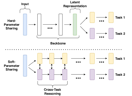
Figure 1: Multi-Task Learning has mainly been divided into two architectural design schemes. Hard-parameter sharing (top) splits a shared backbone into task-specific heads which receives input from from the same set of features. Soft-parameter sharing (bottom) uses task-specific networks, but allows information to be shared between them.

Early DL methods involved attaching task-specific heads to a CNN encoder’s latent representation as shown in Fig. 1 (top) [11]. For example, Ubernet [67] introduced a CNN designed to tackle seven CV tasks. Many subsequent studies followed this design [34, 68, 21, 69]. This architecture shares a CNN backbone which gets updated by gradients aggregated by multiple tasks. As a result, all the tasks pull features from this backbone, which makes a global learned representation critical, although not trivial to obtain as different tasks need different representations to perform well. Hence, recent works suggest sharing parameters as part of multi-task encoder-decoder architectures at the decoder level [70, 71, 72, 73, 74] to exchange high-level semantic features. For instance, Prediction-and-distillation Network (PAD-NET) [70] suggest sharing knowledge after predictions and allows the training of a distillation module to learn what to share. [72] expends on this idea whilst incorporating multi-scale prediction for better dense prediction task performance. Similarly, at the prediction level, Pattern-Affinitive-Propagation (PAP) [71] proposes learning pair-wise task relationship to produce affinity matrices for each task to further guide the sharing strategy.

II-B Feature Fusion

This section introduces parameter fusion techniques used in the two most pre-dominant vision models. First, Section II-B1 introduces methods to share parameters across CNNs. Then, Section II-B2 reviews recent attention-based methods to fuse parameters in Vision Transformers (ViTs) [75].

II-B1 CNN Sharing Strategies

Cross-stitch networks [13] introduce a model-agnostic fusion technique. As opposed to the hard-parameter sharing paradigm, in which task-decoders are attached to a shared backbone encoder (Fig. 1 (top)), [13] introduces a soft-parameter sharing paradigm in which task networks are processed independently and through which parameter fusion is executed in parallel at a similar level of abstraction (Fig. 1 (bottom)). Given two task activation maps $\mathbf{A}$ and $\mathbf{B}$, cross-stitch units [13] compute the dot product between a vector representing their respective values $x^{i,j}_{A}$ and $x^{i,j}_{B}$ at a shared location (i, j) and a trainable weight matrix $\mathbf{W}\in\mathbb{R}^{kxk}$ , where k is the number of tasks. The values in $\mathbf{W}$ represent task-specific (diagonal entries) and shared parameters (non-diagonal entries). Eq. 3 illustrates the process for k = 2

$$\begin{bmatrix}\tilde{x}^{i,j}_{A}\\ \tilde{x}^{i,j}_{B}\end{bmatrix}=\begin{bmatrix}w_{AA}&w_{AB}\\ w_{BA}&w_{BB}\end{bmatrix}\begin{bmatrix}x^{i,j}_{A}\\ x^{i,j}_{B}\end{bmatrix}$$ (3)

Despite being a locally-flexible, easy-to-implement and model-agnostic method, its design results in a complex and expensive model. First, studies investigating CNN layers have shown that shallow layers are usually task-agnostic and cross-stitch units would eventually represent such task-agnostic parameters, but at an expensive of training cost. Second, the overall solution is expensive as the training costs increase with the number of tasks and the size of the network.

Sluice Networks [76] generalise cross-stitch units by increasing the flexibility and sharing parameter space. In particular, [76] allows for selective sharing of layers, parameter subspaces and skip connections. To expand on this soft-parameter sharing structure, [77] proposes a solution based on the principle of Discriminative Dimensionality Reduction (NDDR). This principle attempts to minimise the number of features whilst keeping the maximum amount of representative information, similarly to Linear Discriminant Analysis (LDA) or Principal Component Analysis (PCA). Therefore, NDDR [77] formulates the multi-task feature fusion problem as a discriminative dimensionality reduction problem by first concatenating parallel feature maps, then task-specific 1x1 convolutions [78] are run on such representation to perform dimensionality reduction. In addition, the authors employ batch normalisation and $L_{2}$ weight decay to stabilise learning. This method is illustrated in Fig. 2.

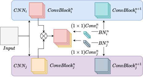
Figure 2: Two task-specific CNN models CNN_i and CNN_j. The NDDR-layer [77] first concatenates the representations of the respective convolutional blocks. 1x1 convolutions are then run on this concatenation, one per task. Last, after batch normalisation, the features are propagated on to the next convolutional block of each model.

As a result, NDDR [77] enables learnable local representation parameter sharing in a similar manner to cross-stitch and sluice networks [13, 76]. However, these techniques hypothesise that all tasks should be processed together, computational cost could therefore be reduced using prior knowledge on task groupings to avoid redundant computation.

II-B2 Attention-based Sharing Strategies

With the advent of the transformer model [79], originally applied to NLP, and subsequently to CV [75], there has been a great improvement in dense prediction tasks in CV [80, 81, 82, 83] due to the non-local feature acquisition inherent to these models as well as their capacity to exploit long-range dependencies. Similar to the aforementioned soft-parameter sharing techniques [13, 76, 77], Multi-Task Attention Network (MTAN) first trains a shared CNN network which is designed to learn general features. This shared framework is attached and at each convolutional operations, a task-specific network with attention modules which learn soft-attention masks over the shared features.

Unified Transformer (UniT) [84] learns a multi-modal encoder-decoder transformer model. UniT [84] learns modality-specific encoders using multi-head self-attention, the modalities are then simply concatenated before a joint decoder performs cross-attention to mix the multiple representations. Similarly, Multi-Task Transformer Network [85] (MulT) performs feature fusion at the decoding level and introduces a shared attention mechanism. Specifically, MulT chooses a reference task $t^{ref}$, then the reference task encoded representation $x$ is used to compute a query $q^{t^{ref}}_{x}$ and a key $k^{t^{ref}}_{x}$. Let us denote $v^{t}$ the values for the other tasks based on the previous stage output. The attention values for this task are then calculated as:

$$A^{t^{ref}}_{x}=softmax\left(\frac{q^{t^{ref}}_{x}\cdot{k^{t^{ref}}_{x}}^{T}}{\sqrt{C_{qkv}^{t^{ref}}}}\right)+B^{t^{ref}}\$$ (4)

Subsequently, for any task $t$, the shared representation is obtained as follows: $\tilde{x}^{t}=A^{t^{ref}}_{x}v^{t}$. The term $x^{t}$ is then used for the multi-head attention.

MTFormer [86] also chooses to compute cross-task interactions at task-specific heads. However, the authors choose to concatenate the projected representations at each transformer block, based on multi-head self-attention operations. To merge the attention maps of $n$ tasks, the authors show it is beneficial to consider self-task attention as a primary task and to consider cross-task attention as playing an auxiliary role in order to perform cross-task feature propagation. To reflect this, the authors choose to reduce the number of projected feature channels $C$ of auxiliary tasks such that $C^{\prime}=\frac{C}{n-1}$, whilst keeping the original dimension for the main task.

Finally, motivated by the success of pyramid-based transformer-based encoded representations for dense prediction tasks [82, 80, 81], InvPT [74] proposes a cross-scale self-attention mechanism for multiple tasks. In this method, the attention maps are linearly combined by learnable weights, the result is also constrained by a residual feature map from the input image.

II-C Knowledge Decomposition

Knowledge Decomposition aims at partitioning a large set of features into smaller and meaningful components. In the context of MTL, one might be interested in recycling large models into smaller multi-task models. First, Section II-C1 reviews how tensor factorization can operate over CNN kernels to construct MTL components. Second, Section II-C2 introduces methods to transfer information from a large single-task teacher model to a smaller multi-task student model. Last, Section II-C3 reviews how adapters can be used to achieve multi-task continual learning by fine-tuning a large single-task model.

II-C1 Tensor Factorization

Section II-A1 reviewed solutions employing the low-rank approximation of a multi-task weight matrix using linear models. Deep Multi-Task Representation Learning (DMTRL) [87] generalises this idea to tensors (N-way arrays with $N\geq 3$). In fact, as per the nature of a CNN, kernels are N-way tensors and fully convolutional (FC) layers are 2-way tensors, stacking those by a number of tasks $T$, usually resulting in large tensors. Tensor Factorization (TF) is a generalisation of some form of matrix decomposition, such as Singular Value Decomposition (SVD) [88]. DMTRL [87] accomplishes soft-parameter sharing in a layer-wise manner between parallel and identical CNNs, similarly to [13, 77]. First, single-task CNNs are trained, then layer-wise parameters are concatenated during backpropagation and subsequently fed as input to SVD-based solutions for decomposition. DMTRL [87] uses multiple sharing strategies, including one based on the Tucker Decomposition (TD) [89], to learn parameters of this SVD-based solution to generate the decomposed units.

Further to this strategy, [90] uses the tensor trace norm (the sum of a matrix’s singular values) as a proxy of the tensor rank on the layer-wise parameters’ concatenation. In this way, each CNN is encouraged to use the other network’s parameters. However, these methods have the same drawback as the previously introduced parameter-fusion based techniques [13, 77, 76] as parameters are shared in a layer-wise fashion which introduces constraints including architectural parallelism and locality in the parameter sharing strategy.

II-C2 Knowledge Distillation

Another perspective to parameter sharing is to design strategies based on Knowledge Distillation (KD). KD is a form a model compression that transfers knowledge from a large model to a smaller model. Early KD work in MTL explored how to compress DRL methods. For instance, [91, 92, 93] introduced a policy distillation strategy to derive lighter multi-task policies from task-specific deep Q-network (DQN) policies. However, as per the nature of DRL, these strategies approach tasks for which the set of actions was finite and would therefore struggle in more complex prediction visual tasks. As a result, [70] introduces, as part of a multi-task multi-modal network, a distillation module to merge predictions from intermediate and complementary tasks from different modalities to subsequently pass representations on to task-specific decoders. The variations for this distillation module include cross-prediction reasoning as well as attention-guided mechanisms. Hence, [94] suggests a two-step solution in which: (1) task-specific models are first trained before freezing their respective parameters; (2) a multi-task model is optimized to minimise a multi-loss objective through the use of adaptors (reviewed in Section II-C3) that align task-specific and task-agnostic parameters together in order for the multi-task model to use the same features as the task-specific models. Following a similar strategy, [95] extends this strategy to a self-supervised pre-training procedure through the use of intermediate pseudo-labeling.

Recently, [96] introduces a new alternative to KD, namely, Knowledge Factorization (KF). Instead of distilling knowledge from a task-specific teacher model to a multi-task student model, KF aims at decomposing a pre-trained, large multi-task model into k task-disentangled factor networks modelling both task-agnostic and task-specific parameters of the teacher model. The resulting lightweight networks can be assembled to create custom multi-task models.

II-C3 Adapters

With the aim of learning universal representations that can perform well across multiple domains, [97] introduces residual adapter modules. Adapters are small neural networks that learn to recognise task-specific parameters given a model pre-trained on another task. Inspired by the ResNet [98] architecture where residual connections are introduced across the sequential process of a CNN, adapters are modules attached after each convolutional block that learn to select parameters to be utilised for a downstream task. This presents an alternative to traditional fine-tuning as only the adapters are trained. [97] demonstrates the capacity of adapter modules to maintain performance across 10 domains by just tuning a small portion of domain-specific parameters, and also their capacity to overcome the challenge of learning without forgetting [99].

[100] introduces parallel adapters as a simpler variant and show that only a few parameters need to be re-trained. As opposed to domain learning, [101] shows how adapters can be used in Incremental Multi-Task Learning (I-MTL). As a new task is optimised, [101] trains task-specific adapters to identify what parameters to retrain and Squeeze-and-Excitation [102] modulation blocks perform channel-wise attention. Furthermore, to address the challenges raised by I-MTL, AdapterFusion [103], inspired by the multi-task objective adapter training strategy proposed by [104], introduces a 2-stage algorithm that enables task-specific parameters inside a transformer model to re-use other task-specific parameters contained in adapters. It is worth noting that, apart from the few aforementioned studies, adaptors have been studied far less in CV than in NLP. There is thus scope for exploiting this efficient parameter-sharing more fully in CV applications

II-D Neural Architecture Search

Neural Architecture Search (NAS) generally attempts to find the best network architecture given a specific problem by manipulating neural modules. However, in case of a multi-task objective, NAS can be seen as a way to partition the parameter space. For instance, [105] introduces parameter sharing through soft ordering (as opposed to parallel ordering). The idea is to learn individual weight scalars per shared layers to soft-merge parameters at different depths of a network. This comes down to learning a N-way tensor of task-specific parameters. Alternatively, Multi-gate Mixture of Experts (MMoE) [106] embeds the Mixture of Experts (MoE) framework [107] in MTL by sharing expert task-specific networks and optimising a gating network to select what features to use for each task. Following the same framework, [108] further improves the efficiency and stability of the selection of experts process and demonstrates its significant improvement on large-scale multi-task datasets.

With the aim of learning an even more flexible assembling strategy, evolutionary algorithms have been proposed as a training strategy in which agents are network inference routes consisting of a set of computational blocks [109, 110]. Similarly, to learn large-scale MTL systems that tackle catastrophic forgetting in the I-MTL paradigm, [111] adopts an evolutionary algorithm to dynamically optimise a model each time a new task is added. Moreover, motivated by even more flexible ways to share features, some work has investigated using computational operations inherent to CNN layers as modulation units. For instance, [112] introduces the Gumbel-SoftMax Matrix model by modulating inner components of a layer, and shows how their activation is learned to optimise tasks through logits. Alternatively, [113] shows how routing policies can be learned through the Gumbel-Softmax sampling method [114] taking into account computational resources. Recently [115] uses this trick to integrate the learning of such policies into its programming framework. [116] modulates networks the same way as [114], however stochastic filter groups are introduced as a way to model the distributions, approximated via variational inference [117], over the possible kernel groupings. More recently, Adashare [113] introduced MTL in such architecture search-based systems to model relationships between tasks by studying the partitioned feature space. As a result, recent studies have focused on leveraging these relationships to route information through networks. For instance, [118] incrementally expands on an initially small network, at each step, grouping similar tasks based on a measure of task affinity. Similarly, [119] implements a low-resource, layer-wise sharing strategy driven by NAS, exploiting task affinity measures. In a CV context, [120] leverages hardware-aware NAS [121] together with MTL to improve the accuracy of dense-prediction tasks on edge devices.

III Optimisation Challenges

MTL has underlying optimisation challenges due to it being a Multi-Objective problem. MTL is subject to two major optimization issues. First, overall performance is dependent on the relatedness of the tasks being optimised. Unrelated tasks can have conflicting gradients that will lead to a non-convergence of a multi-task solution. This phenomenon is called negative transfer. Second, multi-objective performance relies on a thorough task balancing problem as respective complexities interfere during training. For example, easier tasks converge faster, resulting in larger gradients being back-propagated across all tasks. This makes the acquisition of aggregated representations for different task gradients non-trivial. This section reviews solutions aiming to tackle the aforementioned challenges. First, Section III-A reviews how individual losses can be adjusted to balance tasks in a MTL training. Second, Section III-B focuses on techniques that directly operate over gradient updates during training. Third, Section III-C reviews techniques directly inspired from Multi-Objective Optimisation to perform gradient-descent under a MTL configuration. Last, Section III-D introduces other task balancing approaches.

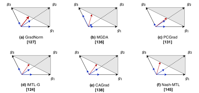
Figure 3: Visualisation of the different gradient update methods in MTL. The blue arrows represent the projections of the task-specific gradient update noted as $g_{1}$, $g_{2}$ and $g_{3}$. The red arrow represents the aggregated gradient update.

III-A Loss-based Techniques

Early work in deep MTL studied a weighted average of the task-specific losses. By considering $\mathit{I}$ tasks and their respective weights $\mathit{w_{i}}$, this model objective can be summarised in Eq. 5.

$$L_{MTL}=\sum_{i}w_{i}L_{i}$$ (5)

Rather than setting weights manually, solutions have been proposed to incorporate the weights into the objective function to adaptively weigh tasks during training. For example, AdaLoss [122] suggests adaptively tweaking weights in such a way that they are inversely proportional to the average of each loss in order to project losses onto the same scale. Alternatively, [68] introduces learnable scalar parameters into the minimisation objective. The authors derive their loss weighting strategy based on the Homoscedastic (or task-dependent) uncertainty which captures the uncertainty of a model, this type of uncertainty is invariant to different inputs. The authors follow a Gaussian likelihood maximisation setting and show that the loss optimisation given two tasks can be approximated as shown in Eq. 6.

$$L_{uncert}(W,\sigma_{1}.\sigma_{2})=\frac{1}{2\sigma_{1}^{2}}L_{1}+\frac{1}{2\sigma_{2}^{2}}L_{2}+log\sigma_{1}\sigma_{2}$$ (6)

Following the same strategy, [123] suggests a slight difference in the $log$ regularisation term, by changing it to $ln(1+\sigma)$. This is to prevent values of $\sigma<1$ yielding negative loss values. We refer to this method as revised uncertainty. However, uncertainty-based task balancing strategies have certain drawbacks and in practice, task-wise terms need to be changed in Eq. 6 depending on the type of task (classification or regression) and depending on the task-specific loss. As a result, IMTL [124] introduces a hybrid method using both gradient methods and adaptive loss tuning. The loss component IMTL-L updates task-specific parameters and learns task-wise scaling parameters $s_{t}$ by minimising a function $g$ for each task $t$ as demonstrated in Eq. 7.

$$g(s)=e^{s}L(\theta)-s$$ (7)

Eq. 7 shows that each task loss is scaled by $e^{s}$ and regularised by the term $-s$ to avoid trivial solutions. In practice, this technique allows tasks to all have comparable scales. Moreover, as opposed to uncertainty weighting [68], IMTL-L does not bias towards any type of task such as regression or classification. Alternatively, [125] introduces a Geometric Loss Strategy (GLS), using the geometric loss to weigh $n$ individual losses. The geometric loss is invariant to individual loss scales which makes it an easy way to balance tasks, as shown in Eq. 8

$$L_{geometric}=\Pi_{i=1}^{n}\sqrt[n]{L_{i}}$$ (8)

Additionally, the authors introduce a variant to focus on $m$ ($m<n$) ‘more important’ tasks and therefore attribute more weighting to these as demonstrated as in Eq. 9,

$$L^{\prime}_{geometric}=\Pi_{i=1}^{n}\sqrt[n]{L_{i}}\times\Pi_{j=1}^{m}\sqrt[m]{L_{j}}$$ (9)

Alternatively, balance of tasks can be achieved through averaging task weights over time by considering the rate of change in the respective task-specific loss. [126] introduces Dynamic Weight Average (DWA). DWA [126] calculates a specific task-specific weight $\lambda_{k}$ for a task $k$ by obtaining a relative descending rate compared to other tasks with respect to the previous iteration (averaged over multiple epochs) as in Eq. 10

$$\lambda_{k}(t)=\frac{Kexp(w_{k}(t-1)/T)}{\sum_{i}exp(w_{i}(t-1)/T)},w_{k}(t-1)=\frac{L_{k}(t-1)}{L_{k}(t-2)}$$ (10)

where $T$ is a temperature parameter controlling the stiffness of the weighting distribution and $K$ ensures that $\sum_{i}\lambda_{i}(t)=K$.

More recently, Random Loss Weighting (RLW) [127] has drawn task-specific weights from a probability distribution at each epoch before normalising them and shows comparable results to SOTA loss-weighting strategies. As a result, [127] provides a more generalisable solution than the baseline (Eq. 5), due to its additional randomness. Finally, [51] provides benchmark results comparing Single Task Learning (STL) to DWA [126], uncertainty [68] and revised uncertainty [123] and suggests that, given careful task selection, the revised uncertainty method [123] generally performs best but suffers when there is lack of training samples.

III-B Gradient-based Techniques

Weighting losses is an indirect way of changing the model’s gradients. Therefore, a line of work has investigated how to optimise MTL models by directly operating over the gradients. Throughout this section, we refer to the illustration in Fig. 3 which provides a visualisation of the gradient update techniques introduced by the presented methods. Formally, the problem is that during multi-task optimisation, a subset of parameters $\theta$ is shared across multiple tasks, as a result, $\theta$ generally receives gradient updates to optimise all tasks at once. In practice, this is achieved by finding an aggregated representation of the vectors. However, finding such representation is not trivial as task-respective gradients might conflict. Hence, GradNorm [128] proposes a method that balances training by automatically tuning the gradient magnitudes. Considering a subspace of weights of a model $W$ (generally chosen as the last shared layer for computational purposes), GradNorm [128] defines the $L_{2}$ norm of the gradient for a particular weighted task loss i, and similarly defines $\overline{G_{W}}(t)$ the average gradient norm across all tasks at time $t$. Additionally, GradNorm [128] defines training rates as $\widetilde{L}_{i}(t)=L_{i}(t)/L(0)$, the loss ratio for a task $i$ at time $t$ and defines a relative training rate for a task $i$ as shown in Eq. 11:

$$r_{i}(t)=L_{i}(t)/E_{task}[\widetilde{L}_{i}(t)]$$ (11)

Subsequently, GradNorm [128] calculates new task-specific gradients for the weight subspace $W$ based on the update rule shown in Eq. 12:

$$G_{W}^{i}(t)=\overline{G}_{W}(t)\times[r_{i}(t)]^{\alpha}$$ (12)

where $\alpha$ is a hyper-parameter controlling the force of traction towards a similar training rate for all tasks. This method, by directly operating over gradients during training, adaptively tunes the speed to which tasks are being trained. However, solely balancing tasks does not prevent conflicting gradients (negative transfer).

GradDrop [129] proposes adding a modular layer that operates during back-propagation to first select a sign (positive or negative) based on the initial distribution of gradient values. It then proposes masking out all gradient values of the opposite sign. Similarly, [130] leverages auxiliary tasks in order to optimise a main task. During training, [130] only minimises the auxiliary losses if their gradient update at epoch $t$ is non-conflicting with the main task gradient update. Specifically, [130] uses the cosine similarity to measure the gradients relation. Conceptually, if the cosine similarity between the main and auxiliary gradients is positive, it suggests that the auxiliary loss should be minimised alongside the main loss, otherwise, it should not. [131] uses a similar strategy in a more conventional MTL setting, in which multiple tasks are optimised simultaneously. [131] uses the cosine similarity to ensure shared gradients are near orthogonal, leading to a non-destructive training between tasks. Unlike [131] which ensures ‘near orthogonal’ properties of the gradients via the minimisation of the loss, PCGrad [132] projects the conflicting gradients of task $i$ onto the normal plane of task $j$ as shown in Fig. 4 (b). Formally, such projection can be defined as in Eq. 13:

$$\Delta g_{i}=g_{i}-\frac{g_{i}\cdot g_{j}}{\lVert g_{j}\rVert^{2}}g_{j}$$ (13)

However, imposing such strong orthogonality constraint upon gradients implies that all tasks at hand should benefit from similar gradient interactions, ignoring complex relationships and destructing natural optimisation behaviour. Moreover, PCGrad [132] stays idle when the gradients have positive cosine similarity, which still might not be optimal as a more desirable similarity (closer a positive cosine similarity) might be preferred. Hence, GradVac [133] leverages both directions and magnitudes in an adaptive strategy. Specifically, given two tasks $i$ and $j$, a similarity goal $\phi^{T}_{i,j}$ is fixed between two gradients $\mathbf{g_{i}}$ and $\mathbf{g_{j}}$ such that $\phi^{T}_{i,j}>\phi_{i,j}$ for which $\phi_{i,j}$ is the cosine similarity, as computed in PCGrad [132]. To achieve this, GradVac [133] derives the projection equation (Eq. 13 by fixing the gradient of $\mathbf{g_{i}}$ and rather estimates the weight of $\mathbf{g_{j}}$ via the Law of Sines in the gradients plane. This process can be summarised as in Eq. 14:

$$\Delta g_{i}=g_{i}+\frac{\lVert g_{i}\rVert(\phi_{ij}\sqrt{1-\phi_{ij}^{2}}-\phi_{ij}\sqrt{1-(\phi_{ij}^{T})^{2})}}{\lVert g_{j}\rVert\sqrt{1-(\phi_{ij}^{T})^{2}}}\cdot g_{j}$$ (14)

Furthermore, using an Exponential Moving Average (EMA) (similar to DWA [126]), $\phi^{T}_{ij}$ is estimated in an adaptive manner during training, over a subset of shared parameters $\mathbf{w}$ belonging to the same layer as illustrated in Eq. 15:

$$\Delta\phi_{ijw}=(1-\beta)\phi^{t}_{ijw}+\beta\phi^{t-1}_{ijw}$$ (15)

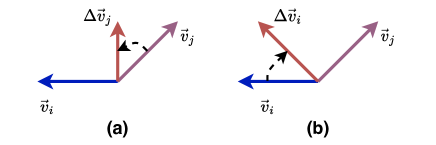
Figure 4: Conflicting vectors (with negative cosine similarity), where $\vec{v}_{i}$ and $\vec{v}_{j}$ represent task-specific updates. In case (a) PCgrad [132] projects $\vec{v}_{j}$ onto the normal space of $\vec{v}_{i}$ resulting in $\Delta\vec{v}_{j}$. In case (b), PCgrad [132] oppositely projects $\vec{v}_{i}$ onto the normal space of $\vec{v}_{j}$. The resulting projections are later added to update the model parameters.

Similarly, [124] suggests a hybrid method leveraging both loss and gradient tweaking, IMTL [124] chooses, in their gradient component IMTL-G, to make all the projections from each task equal to balance the tasks. Recently, RotoGrad [134] proposed a solution to both homogenise gradients magnitude and resolve conflicting ones. To achieve this, a 2-step algorithm is implemented. The first step consists in homogenising the gradients such that the tasks that have progressed the least are encouraged to learn more. Therefore, to project the gradients $\mathbf{G_{k}}$, for a task $k$, Rotograd [134] assigns weights to gradients such that their weighted combination is $\mathbf{C=\sum_{k}\alpha_{k}\lVert G_{k}\rVert}$. Precisely, $\alpha$ is adaptively calculated every $i^{th}$ iteration as shown in Eq. 16:

$$\alpha_{k}=\frac{\lVert G_{k}\rVert/\lVert G_{k}^{0}\rVert}{\sum_{i}\lVert G_{i}\rVert/\lVert G_{i}^{0}\rVert}$$ (16)

In the second step, Rotograd [134] tunes the gradients by learning a task-specific rotation matrix $\mathbf{R_{k}}$ on the last shared representation $\mathbf{z}$. Hence, $\mathbf{R_{k}}$ aims to maximise the cosine similarity between the gradients across tasks given a batch of size $n$; or equivalently, to minimise the loss function shown in Eq. 17.

$$L_{rot}^{k}=-\sum\left\langle R^{T}_{k}g_{n,k},v_{k}\right\rangle$$ (17)

III-C Multi-Objective Optimisation

Multi-Objective Optimisation (MOO) addresses the challenge of optimising a set of possibly conflicting objectives. This section reviews gradient-based multi-objective optimisation methods applied to MTL. First, Section III-C1 formally defines Pareto optimisation and how it is relevant to MTL under gradient descent techniques. Then, Section III-C2 reviews gradient-descent optimisation solutions applied to MTL.

III-C1 Pareto Optimality

As presented in Section III-A, tuning the task-specific weights is not trivial and usually comes at the cost of computational overhead. One way to remedy this is to reframe the MTL optimisation into a MOO problem. Motivation to use MOO for MTL comes from the fact that global optimality for multiple tasks is unconceivable unless a pair-wise equivalence between tasks exists, which is unrealistic. For a hard-parameter sharing network as depicted in Fig. 1 (top), $\theta^{sh}$ represents parameters that are shared and where $\theta^{s}$ are task-specific parameters. Additionally, $\widehat{L^{t}}(\theta^{sh},\theta^{s})$ is the empirical loss for a specific task $t$ in the task set $T$. Then, a multi-objective loss function can be defined as shown in Eq. 18:

$$\min_{\theta^{s},...,\theta^{T}}(\widehat{L}^{t}(\theta^{sh},\theta^{t}),...,\widehat{L}^{T}(\theta^{sh},\theta^{T}))^{\mathbf{T}}$$ (18)

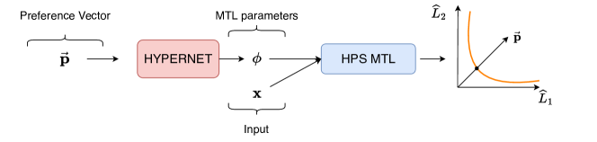
Figure 5: Controllable Pareto MTL [135] approximates the Pareto and allows for real-time trade-off optimisation. A preference vector is sampled using Monte-Carlo methods. This vector is given as input to a Hypernet which outputs the parameters of Hard-Parameter Sharing (HPS) model. The returned Pareto optimal solution is the closest to the preference vector.

Minimising Eq. 18 leads to Pareto-optimal solutions. In other words, in a MTL setting, considering both shared and specific parameters $\theta_{i}^{sh,s}$ and $\theta_{j}^{sh,s}$ for task $i$ and $j$ respectively, a Pareto-optimal solution is one for which a change in $\theta^{i}_{sh,s}$ would damage the performance of task $j$ and vice-versa. The set of Pareto-optimal solutions can therefore be considered as a set of trade-offs between tasks. This set is called the Pareto front ($P_{\theta}$).

Pareto optimality has extensively been studied leveraging the Multiple Gradient Descent Algorithm (MGDA) [136] which supports the Karush-Khun-Tucker (KKT) conditions that are necessary conditions for Pareto optimality. [136] demonstrates that minimising Eq. 19 supports the KKT constraints and either leads to null or to a descent direction that improves all tasks.

$$\min_{\alpha^{1},...,\alpha^{T}}\left\{\left\|\sum_{t=1}^{T}\alpha^{t}\nabla_{\theta^{sh}}\widehat{L}^{t}(\theta^{sh},\theta^{s})\right\|^{2}_{2}\right\}$$ (19)

where $\alpha^{t}$ are non-negative scaling factors such that: $\sum^{T}_{t}\alpha^{t}=1$.

III-C2 Gradient Descent Solutions

In a MTL context, [137] shows that MTL optimisation can be regarded as a MOO problem using MGDA and demonstrates that solving Eq. 18 is equivalent to finding the min-norm point in the convex hull formed by the input points. That is, finding the closest point in a convex hull to a query point. As a result, [137] obtains the aggregated projection of the task-specific gradient vector updates. Subsequently, to solve Eq. 18, [137] uses the Frank-Wolfe solver [138] and ensures, with negligible additional training time, the convergence to a Pareto-optimal solution. CAGrad [139] generalises the MGDA algorithm and chooses to ensure the convergence of the MTL objective to the equally weighted average of task-respective losses. To achieve this, CAGrad [139] first obtains an average vector $d$ of individual task updates $g_{i}$. Then, it aims to find an update vector $g_{w}^{t}$ on a pre-defined ball around $d$, which maximises the conflict between ${T}$ tasks defined as: $-\min_{i\in{T}}\langle g_{i},d\rangle$. Furthermore, the authors show the dominance of CAGrad in a semi-supervised setting compared to MGDA [137]. However, this approach ensures the convergence to any point along the Pareto front which might not be representative of the desired task balance, an unbalanced solution might be preferred to enhance a target task. Therefore, Pareto MTL [140] proposes generalising MGDA to generate a set of multiple Pareto optimal solutions along the Pareto front which would serve as different trade-offs to choose from. To achieve this, [140] takes inspiration from [141] and decomposes the objective space into $K$ well-distributed unit preference vectors $u_{k}$ to guide solutions. Formally, this is achieved through a sub-problem to Eq. 18 where a dot-product maximisation constraint is imposed between $u_{k}$ and a given vector $v$ to guide the learning onto a targeted area of the Pareto front. A sub-region is defined as shown in Eq. 20:

$$\Omega_{k}={v\in\mathbb{R}_{+}^{m}|u_{k}^{T}v\leq u_{k}^{T}v,\forall j=1,...,K}$$ (20)

In contrast to its predecessors, [142] suggests generating continuous Pareto optimal solutions along the Pareto front. To achieve this, [142] proposes a 2-stage training algorithm that, in its first stage, generates a single Pareto stationary point $x_{0}$ from a network’s initialisation. Then, a set of points $x_{n}$ is explored along the tangent plane direction $v_{i}$ and the points are calculated as follows: $x_{i}=x_{0}+sv_{i}$ where $s$ is a step size. As a result, a set of directions is obtained. Finally, [142] combines the tangent vectors acquired in the previous step through linear combination to form convex hulls in which Pareto solutions are obtained, resulting in a continuous approximation of a larger Pareto front.

All the solutions introduced thus far in this section initialise network parameters per trade-off, resulting in a large storage demand and making solutions computationally inefficient. Additionally, the generated solutions are either singular [137] or subject to the practitioner’s preferences [140, 142]. To alleviate both issues, [135] proposes utilising a HyperNet [143], a type of neural network that learns to generate the weights of another network, rendering storage less demanding. Additionally, [135] introduces preference-based training to perform trade-off selection in real-time. More specifically, the objective space is sampled into $K$ subspaces (similarly to [142]). Specifically, given a preference vector $\mathbf{p}$, the goal is to find a local Pareto optimal solution within such subspace for which the angle is the smallest to $\mathbf{p}$. To train the network on representative trade-off preference vectors, vectors are sampled using Monte Carlo methods and are given as input to the HyperNetwork $\mathbf{G}$. Then, the network is updated using normal gradient descent with the loss $\widehat{L}(G(p|\theta))$ in which $\theta$ represents the parameters for the MTL network. Specifically, [135] uses a standard hard-parameter sharing strategy and such a process is depicted in Fig. 5. Similarly, along the lines of preference-driven Pareto optimal solution, [144] chooses to directly cast the MOO optimisation as a Weighted Chebyshev (WC) problem which consists of finding the Pareto front by minimising the $l_{+\infty}$-norm between the initialisation point and the Pareto front.

Recently, Nash-MTL [145] suggests a different approach to obtain an Pareto optimal solution. Inspired by the game theory literature, the authors directly aim at obtaining the Nash Bargaining Solution [146]. This solution can be found on the Pareto front and translates to a proportionally fair solution where any change to the state results in a negative update for at least one task. As a result, the authors show that the aggregated update vector can be obtained as in Eq. 21.

$$\theta^{(t)}= \theta^{(t)}-\eta G^{(t)}\alpha^{(t)}$$ (21)

s.t. $$\textit{solve for $\alpha$ : }(G^{(t)})^{\textbf{T}}G^{(t)}\alpha=\frac{1}{\alpha}$$

where $t$ is a training time-step, $\theta$ represents the shared parameter networks, $\theta$ the learning rate. $G^{t}$ is a task-specific vector update matrix with columns $g^{t}_{i},i\in T$. The results obtained by [145] suggest Nash-MTL achieves current state of the art weighting strategy under many MTL configurations.

However, recently [147] instead demonstrated that most MTL optimisation strategies [137, 128, 132, 129] do not improve MTL training beyond what careful choice of scalar weights in MTL weighted average (Eq. 5 can achieve. Rather, [147] identifies MTL optimisation is particularly sensitive to the choice of hyper-parameters.

III-D Other Task Balancing Techniques

III-D1 Stopping Criterion Techniques

Previous techniques balanced tasks either by finding a combination of the task weights or through gradient manipulation to prevent destructive learning. However, these techniques globally penalise some tasks over others by constraining certain parameters in the objective space. Therefore, [148], as part of their solution leveraging multiple auxiliary tasks to perform facial landmark detection, proposes a task-wise early stopping strategy. The intuition is that once a task starts to overfit a dataset, it will harm the main task as it will force the optimisation to be stuck in a non-global optimum. Hence, a task is stopped if its performance, measured as the product between the training error tendency, noted as $L_{tr}$ and the generalisation error w.r.t $L_{tr}$, noted as $L_{val}$, has not exceeded a certain threshold $\epsilon$. Formally, a training error rate $E_{tr}$ is calculated over a patience epoch length $k$ w.r.t a current epoch $t$. Intuitively, the smaller $E_{tr}$, the greater the signal to continue the training for the task as the training loss substantially drops over the period of time $k$ as shown in Eq. 22:

$$E_{tr}=\frac{k\cdot med_{j=t-k}^{t}L_{tr}(j)}{\sum_{j=t-k}^{t}L_{tr}(j)-k\cdot med_{j=t-k}^{t}L_{tr}(j)}$$ (22)

where $med$ represents the median operation. Similarly, $E_{val}$ measures the overfitting w.r.t $L_{tr}$. [148] defines $\lambda$ as an additional learnable parameter to measure the importance of the task’s loss. This process is shown in Eq. 23.

$$E_{val}=\frac{L_{val}(t)-\min_{j=1..t}L_{tr}(j)}{\lambda\cdot\min_{j=1..t}L_{tr}(j)}$$ (23)

Overall, if $E_{tr}\cdot E_{val}>\epsilon$, the stopping criterion is met.

In a MTL configuration in which all the tasks are aimed to be optimised equally, stopping a task might result in catastrophic forgetting. Therefore, [149] proposes a simple dynamic Stop-and-Go procedure that continually checks for task-wise improvement and degradation during training. Precisely, if performance, measured as the task-wise validation loss term for a given epoch $n$, noted as $L_{t}^{n}$, has not met the performance threshold $\epsilon_{stop}$ over the patience parameter $k$ such that $L_{t}^{n\rightarrow k}<\epsilon_{stop}$. Then, task $t$ is set to STOP mode. If during STOP mode, $L_{t}^{n}$ is degraded and meets the degradation threshold $\epsilon_{go}$ such that $L_{t}^{n}<\epsilon_{go}$, then task $t$ is set back within the MTL training and is set to GO mode. In [149], the authors set $\epsilon_{stop}$ to be 0.1% and $\epsilon_{go}$ to be a degradation of 0.5% of the task’s best performance.

III-D2 Prioritisation Techniques

An alternative to balancing the learning of multiple tasks simultaneously is to instead focus on easier or complex tasks to benefit the training for all tasks. For example, [150] chooses to guide their MTL training by gradually incorporating both harder tasks and harder instances into the objective function. By considering a number of tasks $m$ and a number of instances per task $n$, the authors propose a regularisation $f$ over $\mathbf{W}\in\mathbb{R}^{mxn}$ as shown below:

$$f(W,\lambda,\gamma)=-\lambda\sum_{i=1}^{m}\lVert W^{\mathbf{T}}\rVert_{1}+\gamma\sum_{i=1}^{m}\frac{\lVert W\rVert_{2}}{\sqrt{n_{i}}}$$ (24)

in which the first term imposes the $L_{1}$-norm on the instances $n$, leading to sparsity. This is motivated by the fact that easy instances, for which the empirical loss will be small, have bigger gradients. As training continues, gradually increasing $\lambda$ will introduce harder instances. Similarly, the second term imposes the $L_{2-1}$-norm on $\mathbf{W}$, motivated by the fact that harder tasks exhibit larger empirical losses and gradually reducing $\gamma$ will introduce harder tasks as the corresponding vectors in $\mathbf{W}$ will exhibit near-0 vectors.

On the other hand, some works have focused on starting with harder tasks to benefit easier tasks. For instance, [151] proposes a loss weighting strategy leveraging the focal loss [152]. Although the focal loss is primarily intended for classification, [151] suggests using key performance metrics (KPIs) per task $t$ to generalise the method. Specifically, they adjust these task-specific KPIs $\kappa_{t}$ in an EMA approach as shown below:

$$\bar{\kappa}_{t}^{(\tau)}=\alpha\kappa_{t}^{(\tau)}+(1-\alpha)\kappa_{t}^{(\tau-1)}$$ (25)

where $\alpha$ is a discount factor and $\tau$ is the iteration. Therefore, [151] utilises $\bar{\kappa}_{t}^{(\tau)}$ to change the cross-entropy classification probability $\mathbf{p}$ originally defined as shown in Eq. 26:

$$FL(\mathbf{p},\alpha)=-(1-\mathbf{p})^{\alpha}\log(\mathbf{p})$$ (26)

Finally, [151] defines a task difficulty as a combination of the task-specific loss and its respective KPI-based focal loss as shown in Eq. 27:

$$L_{DTP}=\sum_{t=1}^{T}FL(\bar{\kappa_{t}};\gamma_{t})\widehat{L}_{t}$$ (27)

Alternatively, [153] proposes prioritising harder tasks through active sampling (i.e., choosing what data to train a model with at a particular time $t$ during training). More specifically, the model keeps track of two performance estimations: $t_{i}$ and $c_{i}$ which are a target performance and current performance, respectively, for a task $i$. The task performance is measured as follows: $m_{i}=\frac{t_{i}-c_{i}}{t_{i}}$, where a higher value of $m_{i}$ indicates the model is currently bad at task $i$. Therefore, to encourage the model to prioritise harder tasks, a task-wise sampling strategy is modeled by a distribution $p_{i}$ at every $k$ decision steps which is calculated as follows.

$$p_{i}=\frac{\exp^{\frac{m_{i}}{\tau}}}{\sum_{c=1}^{k}\exp^{\frac{m_{c}}{\tau}}}$$ (28)

IV Task Grouping

As explained in Section III, the overall performance of a MTL model heavily depends on the set of tasks. The optimisation space could be simplified by only processing related tasks together. This chapter focuses on how Task Relationship Learning (TRL) can be achieved through Task Grouping (TG).

Thus far, most works relied on human judgment concerning the relatedness of the tasks. However, these assumptions can be mitigated by quantitatively measuring task relationships. Early attempts in this area aimed to model task relationships (TR) based on vectors in a shared low-dimensional subspace. For example, [154] explicitly builds upon MTFL [54] (introduced in Section II-A) and frames the task grouping problem as a mixed integer programming problem. GO-MTL [60] learns a linear combination of task-specific vectors. Later, [155] expands on previous works modelling TRs using matrix-variate normal distribution over task-specific parameters regularisation techniques to identify positive task correlations [156]. However, to embed this regularisation technique into DL, [155] uses the tensor normal distribution [157] as a prior over task-specific tensors and learns task relationships by learning task covariance matrices. Similarly, [106] learns gating networks in a MoE framework to implicitly model task interactions. However, these works model relationships from a high-level perspective and generally poorly describe pair-wise relatedness. To tackle TG, a body of work focused on studying relationship based on Transfer Task Learning (TTL) by directly learning a mapping between the learned parameters for a task $a$ to a target task $b$ in a MTL setting. For instance, Taskonomy [52] introduced a computational approach to perform TG based on finding transfer learning dependencies between tasks. More specifically, [52], after training task-specific networks, the encoder parts of the networks are frozen and transfer task functions and dependencies are estimated via a target task decoder. Motivated by the idea that multiple source tasks can help provide a more meaningful dependency estimation for a mutual source task, the authors include high-order transfers where a mapping function receives the five best representation as inputs (from the five best first-order source tasks mappings), as illustrated in Fig. 6.

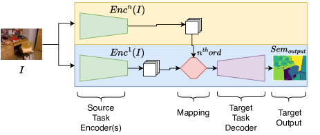
Figure 6: Taskonomy [52] leverages pre-trained encoder(s) (in green) and estimates a mapping (in red) from the latent representation to the input of the target task’s decoder (in purple).

Additionally, Taskonomy [52] derives a vision task clustering architecture and shows that 4 major clusters stand out, namely: 3D tasks, 2D tasks, low dimensional geometric tasks and semantic tasks. Calculating the affinities in such a way is extremely computationally expensive. To alleviate such demand for computation, as opposed to analysing the performance of TTL, Representation Similarity Analysis (RSA) [158] directly investigates the feature maps learned by the task specific networks. The authors choose to leverage RSA to frame the task relationship problem by computing correlation through task-specific inferences on pairs of images. As a result, a dissimilarity matrix is obtained for each task-specific network and a similarity score is obtained through the Spearman’s correlation. However, these latter works only highlight the relationships from a transfer-learning perspective and do not present performance in a multi-task setting. Hence, [159] proposes an alternative to transfer-learning based solutions to highlight task relationships. This alternative is motivated by two findings. First, results obtained by [159] do not show any correlation in the performances between measured task affinities and multi-task learning setting. Second, transfer-learning affinities highlight high-level semantic dependencies as only the bottleneck of the source task encoder is used for the mapping. However, MTL should benefit from clean structural dependencies in all abstraction levels of the features. Instead, the authors in [159] frame this TG problem as an architecture search. Specifically, given an input image, [159] aims to determine the best combinations of encoder backbones and task-specific decoders and perform an exhaustive search over these components. The process is constrained by a search time budget value given a number of tasks $T$. Moreover, [159] optimises the search space using a branch-and-bound procedure and trains between $\binom{T}{2}+T$ and $2^{T}-1$ networks given $T$ tasks before performing TG. However, this search performance is computationally expensive and as a result, [160] directly builds upon this framework and obtains task groups in a single run only. To achieve this, the authors introduce Task Affinity Grouping (TAG) which is a look-ahead algorithm that tracks changes in the MTL loss (in this case, Eq. 5) under different task groupings. Therefore, the authors introduce the notion of task affinity between two tasks $a$ and $b$ defined by $\mathcal{\hat{Z}}_{a\rightarrow b}$ as shown in Eq. 29:

$$\mathcal{\hat{Z}}^{t}_{a\rightarrow b}=1-\frac{L_{b}(X^{t},\theta^{t+1}_{s|a},\theta^{t}_{b})}{L_{b}(X^{t},\theta^{t}_{s},\theta^{t}_{b})}$$ (29)

In which $t$ is the step during the estimation procedure and where the loss $L_{b}$ for task $b$ is parameterised by $X,\theta_{s},\theta_{b}$ which represents the input, the shared parameters and task-specific parameters for task b, respectively. The look-ahead term $\theta^{t+1}_{s|a}$ represents the update of the shared parameters w.r.t. the update on task $a$. Subsequently, a network selection procedure is implemented to maximise the total inter-task affinity score. For instance, for a number of tasks $|T|$ the affinity scores onto a task $a$ are averaged over all the tasks.

$$\mathcal{Z}_{a}=\frac{\sum_{t}^{|T|}\mathcal{\hat{Z}}_{t\rightarrow a}}{|T|},a\in|T|,t\neq a$$ (30)

This problem is NP-Hard and can therefore be solved by a branch-and-bound algorithm.

V Partially Supervised Multi-Task Learning

Methods reviewed so far have mainly focused on a fully-supervised setup which assumes that data is sufficient and all task labels are available. However, this setting is not always realistic as both acquiring data and task labels is an expensive process in certain cases. In practice, the diversity of the task set is limited as required data and labels generally do not co-exist within the same datasets and therefore, not in the same quantities and/or domains. Thus, there is a need to explore MTL in settings that utilise all available source of information. Thankfully, MTL systems can mitigate their data dependency by using available supervisory information of one task to enhance the training of the unlabelled tasks by leveraging task relationships. Therefore, in this chapter, Section V-A reviews how leveraging multiple auxiliary tasks in a self-supervised manner can help obtain a general representation tailored to downstream tasks. Then, Section V-B studies MTL solutions in a semi-supervised settings in which all tasks are optimised. Finally, Section V-C introduces how MTL can be framed in a low-data availability learning paradigm: Few-Shot Learning. Throughout this chapter, we refer to Partial Supervision as an umbrella term encompassing self-supervised learning, semi-supervised learning and few-shot learning.

V-A Self-Supervised Representation Learning

As seen in this review, finding a task-agnostic representation suitable for all the tasks is crucial. However, most previous work in MTL assumed high availability of data and focused on obtaining such representations without diminishing the demand for labels. To remedy this issue, an alternative way to obtain a shared representation is to exploit tasks in a self-supervised fashion. Self-supervised tasks are tasks for which labels can be created without manual annotations. Such tasks hold a strong advantage in the context of MTL as downstream tasks benefit from the representation induced by multiple tasks [13]. As a result, Self-supervised Multi Task Learning (Self-MTL) can be leveraged as a pre-training strategy.

For instance, [161] suggests leveraging 4 self-supervised vision tasks as a pre-training procedure.Relative Position [162] is a task which consists of finding the relative positions of a pair of patches sampled from the same unlabeled image. [162] claims to perform well at this task enhances object recognition. Colorization [163] which requires predicting the original RGB pixel color values given a greyscale image. This task acts as a cross-channel encoder and helps pixel-level dense prediction tasks. The ‘Exemplar’ task [164] where pseudo-classes are estimated for each sample and the network is trained to discriminate between these. This task aims to improving classification properties in the learned representation. Last, Motion Segmentation [165] is a task that learns, given an image $I_{t}$ at a time $t$ to recognise pixels that will move in $I_{t+1}$. This task helps refine the features necessary to both object detection and segmentation prediction through movement cues.

The authors of [161] identify two possible sources of conflict in a Self-MTL setting. First, there are conflicts in the task respective inputs, as for instance, the colorization tasks receive greyscale images whilst others receive RGB images. This results in an network architectural problem. To resolve this conflict, the authors suggest performing input harmonisation by duplicating the greyscale image over the RGB channels. Second, there is conflict in whether the features being trained should generalise to the class at hand or to the specific input image. To resolve this, the authors incorporate their CNN into a lasso regularisation block where each task-specific decoder receives a layer-wise linear combination of the shared backbone convolutional blocks. Hence, a matrix $A\in\mathbb{R}^{TxD}$ is trained to be sparse where $T$ is the number of task-specific decoders and $D$ is the number of convolutional blocks being shared. This regularisation allows the network to factorise the features to enhance the generalisation of the network. [161] presents results matching fully-supervised single-task performance on diverse CV tasks such as classification, detection and depth prediction. The authors’ solution is illustrated in Fig. 7.

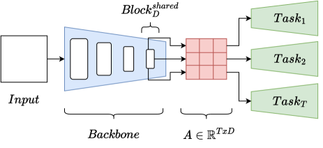
Figure 7: In [161]’s self-supervised solution, the task-specific heads (in green) receive a linear combination of high-level features from the last residual layers of a ResNet-101 [98] encoder. The features are then selected via a matrix $\mathbf{A}$ which is trained to be sparse. This allows for a task-wise factorisation of the learned features to improve the generalisation of the CNN.

MuST [95] uses specialised teacher models to pseudo-label unlabeled multi-task datasets and suggests a pre-training strategy based on the following tasks: classification, detection, segmentation and depth estimation. Subsequently, a multi-task student model is trained on the pseudo-labeled dataset. Fine-tuning on downstream tasks shows that the self-supervised pre-training outperforms traditional ImageNet pre-training baseline [166] and additionally, the authors identify that a large number of tasks and datasets benefit the representation for downstream tasks.

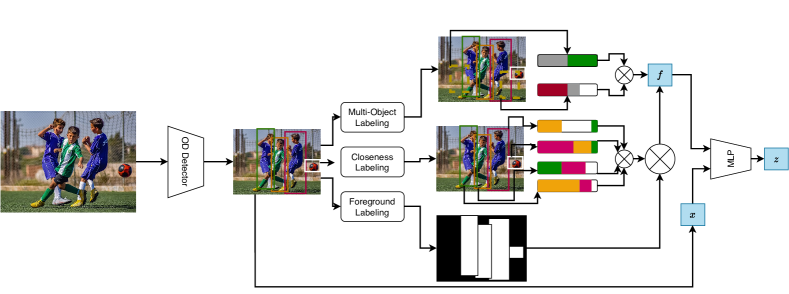
Figure 8: Auxiliary Tasks implemented by [167]. From top to bottom, Multi-object labeling, Closeness labeling, Foreground labeling. Outputs are concatenated and the resulting representation $f$ is fed as input to a Multi-Layer Perceptron (MLP), along with the initial prediction $x$ for refinement.

This capacity to leverage MTL to enhance the shared representation of tasks has motivated applications in diverse areas. For instance, [168] pre-trains a CNN encoder on stereo-paired images from the well-known road object detection dataset KITTI [169] to perform monocular road segmentation. To achieve this, the authors choose to learn two tasks; Drivable Space Estimation and Surface Normal Estimation. Given a stereo-pair of images $(I_{left},I_{right})$, the authors obtain a pseudo disparity map $I_{disparity}$ by using semi-global matching (SGM) [170]. Subsequently, the authors run the Stixel World algorithm [171] which, given a RGB image $I_{RGB}$ ($I_{left}$ or $I_{right}$), exploits the corresponding disparity map $I_{disparity|I_{RGB}}$ to return a semantically segmented representation. MAP estimation is then performed based on the resulting distribution of the predicted pixel labels to extract the drivable area. Subsequently, surface normals are obtained by following the method introduced by [172]. Specifically, given camera-related information such as the baseline distance $D$ and the focal length $D_{focal}$, the previously calculated diversity map $I_{disparity}$ is converted into a depth map $I_{depth}$. This depth map is later projected onto 3D world space $W$ given $D$ and $I_{normals}$ and is obtained via calculating the least-squares plane within $W$ and allocating the planes to neighbouring set of pixels. The authors fine-tune the learned features to perform monocular road segmentation and show impressive results whilst heavily reducing the demand for data.

[167] utilises Self-MTL as a way to refine preliminary Object Detection (OD) predictions. In particular, assuming bounding box labels ${A_{OD}}$ are only available for object detection, 3 auxiliary tasks recycle ${A_{OD}}$ to produce their own respective labels ${A^{t}}$. Such a strategy has two main goals: (1) to learn robust discriminatory features for OD, (2) to refine the preliminary OD prediction. These auxiliary tasks are carefully chosen as follows. First, Multi-Object Labelling randomly produces bounding boxes over the input image, constrained by the fact that one must overlap with at least one Ground Truth (GT) bounding box. Then, labels are assigned to the sampled bounding boxes based on GT Bounding Box area it overlaps the most with. The intuition behind this task is to perform augmentation on the input image to enhance globalisation. Second, Closeness Labeling accounts for the inherent proximity in object classes in an image. This task consists in iterating over the GT bounding box annotations to provide a one-hot encoding based on the proximity of neighbouring GT bounding boxes. Finally, Foreground labeling encodes the foreground and background, assigning 1’s to pixels within GT bounding boxes and 0’s otherwise. These tasks are illustrated in Fig. 8. Information encoded by these tasks is concatenated into a representation $f$ and is used to update the original prediction $x$ via a 1-layer FC layer to obtain a final refined prediction $z$ such that: $z=f\oplus x$.

These methods demonstrate how effectively leveraging multiple self-supervised objectives can improve a shared representation suitable for MTL. Such efficiency has motivated some works to employ Self-MTL for diverse target downstream tasks in CV. For example, [173] suggests a meaningful self-supervised pre-training strategy for Image Aesthetic Assessment (IAA). IAA models, which are usually trained an aesthetic-labeled ImageNet dataset [166], do not provide much information for why an image is not aesthetically good, for example, intrinsic image characteristics (i.e., brightness, blurriness, contrast etc). Therefore, the authors train a comparative network of 2 distorted images, the distortion is chosen as one of the aforementioned characteristics and the networks aim at estimating the type of distortion as well as its intensity in an unsupervised manner. The goal of the MTL system is to recognise the less distorted image. Moreover, additional tasks are added to recognise the type and intensity of the distortion operation applied to the two input images. The authors report a decrease in 47% in the number of epochs necessary for convergence compared to a IAA network pre-trained on Imagenet [166], notwithstanding the reduced need for data.

Alternatively, self-MTL framework has shown state-of-the-art results in real-time applications. For example, SSMTL [174] tackles anomaly detection in videos. Acquiring anomalous labels is difficult and as a result, the authors leverage self-supervised tasks to train a 3D CNN to recognise anomaly in videos. SSTML [174] first runs a pre-trained YOLOv3 [10] to identify objects on a set of object-level frames ${I_{n}}$. Then, the authors choose three tasks to identify anomalous objects. First, irregularity is identified through the arrow of time task, which involves obtaining an abnormal label by training the 3D CNN on the video in reverse mode. Second, motion irregularity detection for which abnormal events are obtained via skipping frames is used to identify irregular motions such as someone running, falling etc. Third, a middle box prediction task is implemented to predict the middle frame. Last, the authors enhance their multi-task 3D CNN through knowledge distillation where the object detector YOLOv3 [10] is trained to predict the last layer of a ResNet-50 [98], which predicts whether the middle box frame is abnormal or not. The key point is that, in the knowledge distillation head, the authors expect a high difference between the object-level predictions of the 3D CNN and the ResNet-50 predictions when an anomaly is observed. The results significantly outperform previous state-of-the-art methods. Moreover, SSMMTL++ [175] recently reviews this framework and further improves it through the introduction of different tasks such as optical flow and advanced architectures such as the ViT [75].

In addition to using multiple auxiliary tasks to enhance the learned representation, multiple modalities can be utilised to provide even more useful sources of information for models to learn. Multi-modal representation learning can be achieved by pre-training on diverse datasets. For instance, [149] obtains a vision-language representation by pre-training on 12 vision-linguistic datasets and shows impressive results on common multi-modal tasks such as visual question answering and caption-based image retrieval. The authors utilise multi-modal self-supervision, inspired by [176], by masking proportional amounts of both image and word tokens and also by performing multi-modal alignment, by predicting if two instances belong together. Similarly, [177] introduces Multi-SSL, a multi-modal (sound and image) pre-training strategy aiming to provide a shared representation for both sound and image modalities that could be used for downstream tasks.

[178] leverages the recent the success of Masked Auto-Encoders (MAEs) [179]. MAEs [179] are asymmetric encoder-decoder models in which the encoder only operates on a small portion (about 15 %) of a patch-wise masked input image and the decoder aims at regenerating the missing patches. In particular, [178] proposes Multi-Task MAE (MultiMAE), a pre-training strategy reconstructing diverse image modalities. To achieve this, given a set of RGB images, image modalities are acquired solely via Pseudo-labeling. First, the depth modality is approximated by running a pre-trained DPT-Hybrid [180], a ViT-based model. Similarly, Semantic Segmentation pseudo-labels are obtained via Mask2Former [181] trained on the COCO dataset [182]. Once these labels are obtained, similar to original MAE [179], the authors sample a large portion of the image modalities divided into 16x16 patches. Subsequently, a number of tokens corresponding to approximately $\frac{1}{8}$ of the entire number of tokens for the 3 modalities (RGB, depth and semantic) are kept visible. The sampling strategy follows a symmetric Dirichlet distribution (with $\alpha$=1), equivalent to a uniform distribution so that no modality is prioritised. Then, the authors perform a 2D-sine-cosine linear embedding on the patches which are fed as input to the multimodal ViT encoder which operates only on the visible tokens, tremendously reducing the cost of computation [179]. For downstream tasks, the multi-modal self-trained encoder can be used to fine tune a single task whilst benefiting from geometrical cues induced by other modalities. This framework is illustrated in Fig. 9.

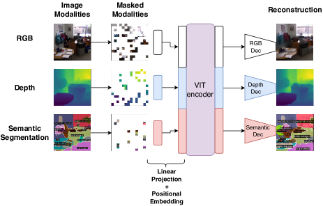
Figure 9: [178] leverages three image modalities, obtained via pre-trained models, as a pre-training strategy. Respective image modalities are patch-wise masked in a similar way as MAE [179]. Subsequently, linear projection and positional embedding are applied on patches. Then, patches are given as input to a shared ViT [75] encoder which processes all the different representations. Finally, task-specific decoders aim at reconstructing each modality.

In addition, Muli-Task Self-Supervised pre-training has been investigated in medical applications [183, 184, 185], in music classification [186] or in NLP for multilingual reverse dictionaries [187].

V-B Semi-Supervised Learning Methods

V-B1 Traditional Methods

[19] proposes the first semi-supervised MTL framework. The framework consists of $T$ classifiers whose parameters share a joint probability distribution based on a soft variant of a Dirichlet Process. This allows for the parameters to be trained together and for the predictions to be obtained all at once. The probability distribution variant retains the inherent clustering property of Dirichlet Processes and as a result, the authors process unlabeled data via Parameterized Neighborhood-based Classification (PNBC). More specifically, the authors perform a Markov random walk over neighbouring data points obtained via supervised training, then, classifiers learn to assign unlabeled data to its closest point. Later, [188] expands on this setting by framing MTL as a clustering problem. To achieve this, after training $T$ linear classifiers, the authors improve their generalisation w.r.t. to their respective data by imposing a norm over the classification weights. Subsequently, the algorithm follows the same procedure, frames the respective classifiers into clusters via K-means clustering and assigns unlabeled points to nearby classifiers within that space. The authors also show this framework can be extended to non-linear classification through the use of kernels. It is worth noting that these traditional methods had a different notion of the MTL problem. In fact, the tasks are classification tasks in which ‘tasks’ are either different datasets [188] or classes, resulting in multi-class classification [19]. As a result, only one loss function is used for the optimisation which significantly differs from the contemporary definition of MTL.

V-B2 Self-Supervised-Semi-Supervised Methods

The methods introduced in Section V-A highlight how multi-task learning can be used with self-supervised auxiliary tasks to minimise the overall training cost and demand for data. This characteristic has motivated numerous works to leverage both semi-supervised learning and self-supervised learning.

As explained in Section IV, some tasks provide global understanding of scene geometry (i.e., surface normals, depth prediction …) and when trained adequately, translate into low-level features tailored for dense prediction tasks. Therefore, there has been effort to investigate these tasks to improve an important CV task: Semantic Segmentation (SS). For instance, [189, 190] use depth prediction as a proxy task for supervised urban scene understanding tasks such as car detection, road and semantic segmentation. Similarly, [191] uses both depth estimation and colorization as a pre-training strategy for semantic segmentation in autonomous driving. To expand upon the idea that self-supervised depth estimation (SDE) can be effective to reduce data dependency, [192] introduces three ways to leverage SDE to improve semantic segmentation in a semi-supervised learning paradigm.

First, the authors suggest an active learning strategy based on depth prediction. Specifically, given a set of images of the same domain ${G}$, the authors aim to split it into two image subsets. On the one hand, ${G_{A}}\subset{G}$ will be used for pseudo-labeled annotations for SDE, whilst ${G_{U}}\subset{G}$ is the set of unlabelled images. To obtain these, the authors iteratively choose ${G_{A}}$ through diversity sampling. Precisely, diversity is obtained when the chosen images are most representative of the dataset distribution. In urban scene understanding, this could result in the most frequent types of buildings, cars, bicycles, etc being chosen. To achieve diversity, the authors first populate ${G_{A}}$ with a random image and iteratively select the farthest $L_{2}$ distance between two sets of features of both ${G_{A}}$ and ${G_{U}}$. The features correspond to the same layer $l$ of a pre-trained SDE network $f_{SDE}(\theta,I)$. Formally, the active learning procedure can be formulated as in Eq. 31:

$$G_{A_{n+1}}=\arg\max\min\lVert f_{SDE}(\theta,G_{U})-f_{SDE}(\theta,G_{A})\rVert_{2}$$ (31)

Subsequently, the authors aim to incorporate another important aspect to this active sampling: Uncertainty Sampling which consists in choosing samples that are hard to learn for the current state of the model: formally, instances in ${G_{U}}$ for which the model’s decision is close to the decision boundary. To achieve this, a student model $f^{\prime}_{SDE}(\theta,I)$ is trained on ${G_{A}}$. The authors then measure the disparity, on ${G_{U}}$, of both the predictions of $f_{SDE}$ and those of $f^{\prime}_{SDE}$. Formally, the difference is calculated using the $L_{1}$ distance as shown in equation Eq. 34:

$$E(i)=\lVert log(1+f_{SDE}(\theta,I))-log(1+f^{\prime}_{SDE}(\theta,I))\rVert_{1}$$ (32)

The authors choose to use the $log$ regulator to avoid close-range objects dominating the disparity difference. Conceptually, sampling based on these two characteristics benefits from diversified, complex and representative instances which results in a decreased demand for data samples.

Second, inspired by the success of pair-wise data augmentation in CV [193, 194], [192] introduces DepthMix as a way to further reduce this labeling demand. In this method, considering 2 images $I_{source}$ and $I_{target}$, the goal is to learn a binary mask $M$ over $I_{source}$. Specifically, the positive values in $M$ represent regions to be copied over $I_{target}$. As a result, the augmented image $I_{augmented}$ is obtained as shown in Eq. 33:

$$I_{augmented}=M\odot I_{source}+(1-M)\odot I_{target}$$ (33)

where $\odot$ is the element-wise product. In contrast to existing data augmentation methods, [192] leverages depth to avoid violating geometric semantic relationships between objects. For example, it is undesirable to have a distant object in $I_{source}$ to be copied onto the forefront of $I_{target}$, or worse, to result in geometrically implausible situations like a close-range motorbike copied on the top of a close-range car. To mitigate this problem, the authors use depth predictions for both images noted as $D_{source}$ and $D_{target}$. To achieve this, given a shared location $(x,y)$, $M$ is constrained to select only pixels for whose depth values are smaller on $I_{source}$ than on $I_{target}$. This process is demonstrated in Eq. 34:

$$M(a,b)=\left\{\begin{array}[]{ll}1&\mbox{if }D_{source}(a,b)<D_{target}(a,b)+\epsilon\\ 0&\mbox{otherwise}\end{array}\right.$$ (34)

where $\epsilon$ is a small noise value to avoid conflicts of objects that are the same depth plane on both images such as curb, road and sky.

The final component introduced in [192] is a semi-supervised MTL network to perform both Depth Estimation and Semantic Segmentation.

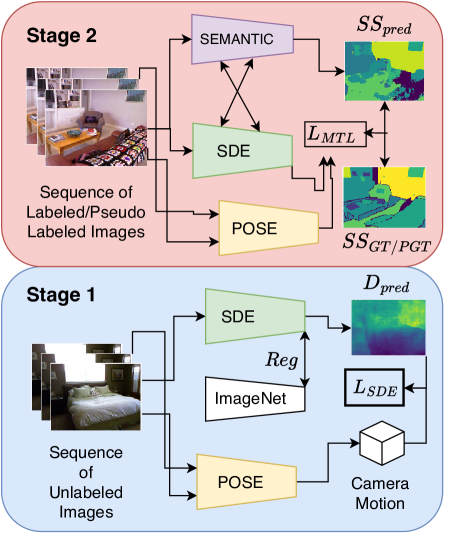
Figure 10: [192] leverages Self-supervised Depth Estimation (SDE) to improve Semantic Segmentation. The training strategy is composed of two stages. In stage 1, a camera pose estimation network along with a SDE encoder is trained on an unlabeled sequence of images. Then, in stage 2, semantic segmentation is added and is trained on a sequence of images containing a mixture of labeled and pseudo-labeled images.

The authors train their MTL network in 2 stages. The first stage is depth pre-training. This stage consists in a self-supervised training for both depth estimation and pose estimation on an unlabeled sequence of images. As part of this procedure, a shared encoder $f_{\theta}^{E}$ is initialised with ImageNet [166]. Additionally, in order not to forget the semantic features during training, the initialised features, noted as $f_{I}^{E}$, serve as a regulator for the SDE pre-training and the authors use the $L_{2}$-norm in order to guide the multi-task representation. The resulting loss term is formulated as shown in Eq. 35:

$$L_{SDE}=\lVert f_{\theta}^{E}-f_{I}^{E}\rVert_{2}$$ (35)

In the second stage, the authors introduce semantic segmentation to form a semi-supervised network. In this stage, the network is trained on depth estimation on both labeled and pseudo-labeled (using the mean teacher algorithm [195]) instances. Their solution is illustrated in Fig. 10. As a result, the authors manage to achieve 92% accuracy on a baseline fully-supervised model whilst using 1/30 of labeled image segmentation instances. Furthermore, whilst using 1/8 of the SS labels, it outperforms this supervised baseline by a small margin. The authors then improve their solution to perform domain adaptation [196].

Recently, [197] leverages both depth and surface normals estimation to improve on semantic segmentation. In addition, the authors show how Nash-MTL [145] can lead to efficient solutions.

V-B3 Generative Modeling

Recent advances of general self-supervised methods such as adversarial training with Generative Adversarial Networks (GANs) [198], as well as the ability of generative modeling to learn useful visual representations from unlabeled images [199], have motivated the investigation of generative modeling in MTL to lower the demand for labeled data [200, 201].

For example, [16] proposes a self-supervised semi-supervised MTL ($S^{4}MTL$) solution leveraging adversarial learning and semi-supervision to teach simultaneously two commonly tackled CV tasks, namely: Image Classification (for diagnostic classification) and Semantic Segmentation. By considering two datasets, one labeled $D_{A}$ and one unlabeled $D_{U}$, the authors define their respective losses as $L_{A}$ and $L_{U}$. If $\theta$ and $\upsilon$ define the network parameters for semantic segmentation and diagnostic classification respectively, then the overall objective can be summarised as:

$$\min_{\upsilon,\theta}L_{A}(D_{A},(\upsilon,\theta))+\alpha L_{U}(D_{U},(\upsilon,\theta))$$ (36)

where $\alpha$ is a positive weight for the unsupervised loss. Subsequently, the authors train two networks: $G$, a mask generator for semantic segmentation and $D$ a classifier which is trained in an adversarial fashion. These two networks are divided into two branches. For supervised images, $G$ wants $D$ to maximise the likelihood of the segmentation masks given a regular image-label pair. For the unsupervised images, the model performs a transformation $t(x)$ over the input image $x$ such as rotation to enable $G$ to make predictions. Such a framework is illustrated in Fig. 11.

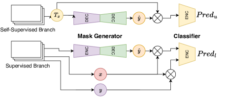
Figure 11: In [16]’s solution, a two-branch MTL network shares the same Generator and Discriminator trained in an adversarial fashion. For the self-supervised branch, a transformation $T_{x}$ is applied to the input image.

Using this framework, the model is claimed to outperform fully-supervised single task models whilst diminishing the availability of data/label up to 50%.

[18] extends on this framework and introduces SemiMTL. This method performs urban scene segmentation and depth estimation. However, the authors leverage multiple datasets in a heterogeneous (trained on different datasets) MTL framework and train their discriminator in a domain-aware fashion to compensate for the domain shift inherent to this environment. To do this, the authors add a inter-domain loss between the labeled dataset $A$ and unlabeled dataset $B$ which can be illustrated as below:

$$L_{inter}^{t}=-\sum_{h,w}\log(D_{t}(\hat{y}^{B}_{t})^{(h,w,y^{A}_{t})})$$ (37)

where the ground-truth value for the datasets $A$ and $B$ for an arbitrary task $t$ is noted as $y^{A}_{t}$ and $y^{B}_{t}$, respectively. Moreover, the respective two predictions are noted $\hat{y}^{A}_{t}$ and $\hat{y}^{B}_{t}$. Conceptually, the loss in Eq. 37 aligns the unlabelled task prediction $\hat{y}^{B}_{t}$ onto the labelled task ground-truth $y^{A}_{t}$ to compensate for domain shifts. Additionally, the authors introduce different ground-truth and prediction alignment strategies such as aligning the unlabelled prediction $\hat{y}^{B}_{t}$ onto the labelled task prediction $\hat{y}^{A}_{t}$ or aligning $\hat{y}^{B}_{t}$ onto the intersection of the labelled ground-truth $y^{A}_{t}$ and prediction $\hat{y}^{A}_{t}$.

V-B4 Discriminative Methods

Discriminative methods aim at determining boundaries between image representations by directly comparing them. This section focuses on MTL works introducing this technique under semi-supervised training paradigms. One type of discriminative method that has shown great success in many CV tasks is Contrastive Learning (CL). CL was originally introduced by [202]. It involves learning a joint-space in which similar pairs of images are close to each other and in which different pairs are far part. Momentum Contrast (MoCo) [203] extends this concept for unsupervised visual learning and sees this framework as a dictionary look-up problem where an image $I$ is encoded by a network $f$, this is denoted as the query $q=f(I)$. Then, a queue of size $n$ of image representations ${I_{k}}$, or keys, chosen as the preceding mini-batch, which are encoded by a momentum encoder $f_{m}$ are compared $k_{n}=f_{m}({I_{k}})$. Subsequently, the matching key $k_{+}$ is noise-augmented. Finally, $f$ is updated via the InfoNCE [204] loss shown in Eq. 38.

$$L_{InfoNCE}=-\log\frac{\exp(q\cdot k_{+}/\tau)}{\sum_{i=1}^{N}\exp(q\cdot k_{i}/\tau)}$$ (38)

SimCLR [205] suggests a simpler version comparing diverse augmented versions of the same image, however it requires larger batch sizes.

Table I: MTFormer[86] treats a target task annotations as few-shot samples whilst keeping two other tasks fully-supervised.
Results are reported on the PASCAL dataset [206].

Method		Few-Shot Task		SS $\uparrow$		Human Part Seg. $\uparrow$		Saliency $\uparrow$
				mIoU $\uparrow$		mIoU $\uparrow$		mIoU $\uparrow$
STL		SS		3.34		63.90		66.71
MTFormer [86]		SS		35.26		64.26		67.26
STL		Human Part Seg.		71.17		11.27		66.71
MTFormer [86]		Human Part Seg.		73.36		51.74		67.74
STL		Saliency		71.17		63.90		44.39
MTFormer [86]		Saliency		76.00		66.89		55.55

Motivated by the aforementioned approaches, MTSS [207] suggests a simple, yet effective, semi-supervised MTL framework to optimise a discriminative self-supervised auxiliary task and a supervised main task simultaneously.

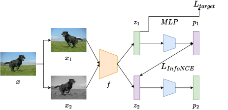
Figure 12: [207] suggests to perform two augmentations of the same image. Each of the representations are encoded through the CNN encoder $f$, resulting in representations $z_{1,2}$. Whilst one representation (i.e $z_{1}$) can be processed by the main task, the InfoNCE [204] loss is minimised between $z_{2}$ and the encoded representation $p_{1}$.

Specifically, the authors choose to maximise the similarity between two different views of the same image. First, two augmentations on the same image are performed, these views are $x_{1}$ and $x_{2}$. Then, a shared CNN classifier process them leading to two representations $z_{1}$ and $z_{2}$. One, for example $z_{1}$, is chosen to be processed by the supervised main task. Similarly to SimCLR [205], the authors choose to attach a Multi-Layer Perceptron (MLP) in order to map representations to a similar space, let us denote the resulting representations as $p_{1}$ or $p_{2}$. Finally, the cosine similarity $D$ between $p_{1}$ and $z_{2}$ is calculated as shown below:

$$D(p_{1},z_{2})=-\frac{p_{1}}{\lVert p_{1}\rVert_{2}}\cdot\frac{z_{2}}{\lVert z_{2}\rVert_{2}}$$ (39)

to minimise the cosine similarity between the representations of augmented views. The symmetric auxiliary loss, introduced by BYOL [208] and depicted in Eq. 40, is used as follows:

$$L_{aux}=\frac{1}{2}D(p_{1},z_{2})+\frac{1}{2}D(p_{2},z_{1})$$ (40)

This auxiliary loss is then added to the overall MTL objective. The semi-supervised framework is depicted in Fig. 12.

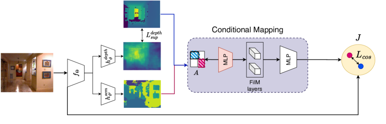
Figure 13: Considering an input image for which only the depth ground truth is available, [17] performs cross-task consistency and maps the depth ground-truth to the semantic segmentation prediction to a joint space $J$ through a conditional mapping network (in purple). The cosine distance between the two representations is minimised.

Another recent task discriminatory approach, Cross-Task Consistency (XTC), is introduced by [209]. Conceptually, this notion comes from the dependency between two tasks. For instance, in the context of urban scene semantic segmentation with depth estimation, there would be inconsistency if depth estimation evaluated a flat surface where a car is detected. Therefore, [209] aims to compute task pair-wise mapping to map the prediction from a source task to the label of the target task. However, each of those mapping functions are parameterised by two DNNs and leverage labels from each task. To mitigate the use of labeled data, [17] leverages cross-task relations in a semi-supervised framework. Specifically, [17] suggests a framework to map the prediction of an unlabeled task $\hat{y}^{s}$ to the ground truth of another task $y^{t}$ through an adaptive encoder which embeds only shared parameters. Therefore, the two representations $\hat{y}^{s}$ and $y^{t}$ are mapped on to a joint space and their cosine distance is minimised.

The authors in [17] leverage XTC in their framework for semantic segmentation, depth estimation and surface normals estimation. Let us consider a partially-supervised image $I$, for which only $y^{depth}$ or $y^{semantic}$ is available. $I$ is then processed through a shared backbone network $f_{\Theta}$ to which task-specific decoders $h_{\vartheta}^{depth}$ and $h_{\vartheta^{\prime}}^{semantic}$ are attached. The obtained predictions are noted as $\hat{y}^{depth}$ and $\hat{y}^{semantic}$. For the sake of illustration, let us consider $\hat{y}^{semantic}$ not to be labelled and therefore to leverage the available ground-truth from the depth estimation task. Now describing the XTC mechanism, let us consider a matrix $A$ for which entries correspond to $source\rightarrow target$, (in our example, $A[semantic,depth]=1$) and all other entries are 0. An auxiliary network $k_{\theta}$ is used to conditionally parameterise a mapping network $m_{\psi}$. Similar to [210], $k_{\theta}$ is used to update the layers of $m_{\psi}$. This mechanism is to allow for a conditional source-to-target mapping. The two resulting representations are then projected on to the same joint-space $J$. The authors use the cosine similarity to minimise their distance. Additionally, to avoid trivial mappings, the features from $f_{\Theta}$ are used as a regularisation term of the distance between the mapping function’s output and the encoded features $f_{\Theta}(I)$. The explained mapping is illustrated in Fig. 13.

V-C Few-Shot Learning Methods

Few-Shot Learning (FSL) is a learning paradigm that aims to learn unseen classes from a few examples. This training paradigm is motivated by the fact that humans do not need hundreds or thousands of exemplar images to learn to recognise an object. Typically, FSL systems consist of two stages. First, a general feature extractor is learned from a large annotated dataset in a stage called meta-training. Second, an adaption strategy is used to classify the new sample/class (also known as the query sample) based on a small labeled support set. This stage is called meta-testing. A similarity function is then used on the support set to identify the matching class given the query sample. Traditionally, in FSL-MTL, the goal is to adapt to unseen classes for a specific task within a MTL model. In the context of MTL, cross-task interactions within a multi-task system could help enhance the generalisation to the few-shot target task. In fact, [211] shows that MTL models generally focus on tasks that have the least training samples, which is due to the feature sharing process across tasks.

Recently, the FSL literature has heavily focused on the initial meta-training stage in which multiple datasets serve to train a model to obtain global representations for a target few-shot task, most commonly being image classification. For example, [212] suggests training such a model in a MTL fashion by leveraging self-supervised tasks (similar to solutions introduced in Section V-A), on both labelled and unlabelled images. The shared encoder is regularised by the contrastive learning method: BYOL [208]. Subsequently, the MTL system is evaluated on traditional few-shot image classification.

MTFormer [86] suggests different dense prediction tasks as few-shot tasks and evaluates a MTL system leveraging a cross-task attention mechanism at the decoder level of a ViT [75] on the PASCAL dataset [206]. The authors evaluate three tasks, in turn, as a few-shot sampled task by randomly sampling about 1 % of the annotated data for the few-shot task and keeping all available labels for other tasks. MTFormer [86] chooses to evaluate Semantic Segmentation, Human Part Segmentation and Saliency Detection which consists of identifying interesting points in an image (points that the human eye would focus on straight away). The results, presented in Table I, display an impressive improvement over the single-task FSL baseline. This improvement is explained by two techniques: the feature propagation across tasks to enhance the few-shot task representation, and the use of CL in [86], in which different task representations of the same image are considered as positive samples, which further reinforces the shared representation’s quality.

Visual Token Matching (VTM) [213] proposes a continual few-shot learning framework for dense prediction vision tasks. In this setting, a universal few-shot learner can learn new dense prediction tasks given extremely limited labelled task images, most often only using 10 labelled examples of image-label pairs. VTM employs a encoder-decoder architecture using ViT encoders [75] to encode both image and label. As a way to propagate features across the model hierarchies, the authors perform token matching using an attention mechanism similar to MTFormer [86]. More specifically, given a target few-shot task $t$, a query image $Q_{t}$ and support set of image-label pairs of length $N$ ($(X,Y)^{1...N}_{t}$), a task-specific shared encoder $f_{t}$ is used to process both $Q_{t}$ and $X^{i}_{t}$. On the other hand, a label encoder $g$ is used to encode $Y^{i}_{t}$. Subsequently, the token matching mechanism based on attention operates on ViT blocks representations. The block-wise query label predictions are then concatenated before a classification head provides the final prediction. Finally, the results reported by [213] suggest similar strategies should be elevated to the simultaneous MTL settings.

Table II: Self-supervised MTL

Method	Dataset	Tasks	Labels	Backbone	SS		OD		C
					mIoU $\uparrow$		mAp $\uparrow$		Top-1 Acc $\uparrow$	Top-5 Acc $\uparrow$
[161]	ImageNet [166]	C	-	Resnet-101 [98]	-		-		-	85.10
	Pascal VOC [206]	OD	-	Resnet-101 [98]	-		74.17		-	-
[168]	KITTI [169]	SS (Drivable Space)	-	VGG-net [98]	94.23		-		-	-
[167]	Pascal VOC [206]	OD	-	Fast R-CNN [6]	-		77.5		-	-
	COCO [182]	OD	-	Fast R-CNN [6]	-		34.6		-	-
[192]	Cityscapes [214]	SS	1/30	ResNet [98]	62		-		-	-
[178]	NYUv-2 [215]	SS	-	ViT [75] (RGB-only)	50.6		-		-	-
	NYUv-2 [215]	SS	-	ViT [75] (RGB+Depth)	53.6		-		-	-
	ImageNet-1K [166]	C	-	ViT [75] (RGB-only)	-		-		83.3	-
[197]	NYUv-2 [215]	SS	-	ResNet [98] (Nash-MTL)	80.0		-		-	-
	NYUv-2 [215]	SS	-	ResNet [98] (Unc.W)	74.8		-		-	-

Table III: NYUv2 and Cityscapes

Dataset	Method	SS		Depth			SN
		mIoU $\uparrow$		aErr $\downarrow$	AbR $\downarrow$		mErr $\downarrow$
NYUv2 [215]	$STL_{SS}$	37.45		-	-		-
	$STL_{Depth}$	-		0.61	-		-
	$STL_{SN}$	-		-	-		25.94
	$MTL_{CNN}$	36.95		0.55	-		29.5
	[17] MTPSL (1/3)	28.43		0.63	-		33.01
	[17] MTPSL (one)	31.00		0.51	-		28.58
Cityscapes [214]	$STL_{Seg}$	74.19		-	-		-
	$STL^{SegNet}_{Depth}$	-		0.012	-		-
	$STL^{ResNet}_{Depth}$	-		-	0.41		-
	$MTL_{CNN}$	73.36		0.016	-		-
	[17] MTPSL (one)	74.90		0.016	-		-
	[17] MTPSL (1:9)	71.89		0.013	-		-
	[17] MTPSL (9:1)	74.23		0.026	-		-
	[18] SemiMTL	71.9		-	0.28		-

VI Datasets & Tools

Section VI-A refers the reader to a list of datasets commonly utilised in MTL for computer vision. Additionally, Section VI-B provides a summary of the results achieved by partially-supervised MTL solutions. Based on these results, we discuss and analyse common trends and suggest interesting paths of exploration to further improve MTL. Last, we introduce a table summarising the different open-source MTL code.

VI-A Datasets

Below is a list of common multi-task CV datasets.

1. Taskonomy. [52] This dataset is the largest multi-task dataset. It contains 4.5 million indoor scene images, each labeled with 25 annotations. These images include: scene annotations, camera information, 2D/3D keypoints, surface normals and various-level object annotations. The foundational work [52] on this dataset performed experiments on 26 diverse tasks.

2. NYUv2-Depth v2. [215] This dataset comprises 1449 labeled images drawn from indoor scene videos for which each pixel is annotated with a depth value and an object class. Additionally, there are 407,024 unlabeled images which contain RGB, depth and accelerometer data, rendering this dataset useful for real-time applications as well.

3. Cityscapes. [214] This dataset consists of 5000 urban scenes. Each image is annotated with pixel-level labels for 30 classes. Additionally, the dataset includes image stereo pairs associated camera shift metadata. Therefore, [214] leverages stereo-paired information to produce accurate depth labels. As a result, Cityscapes [214] is typically used as a 7-class semantic segmentation class and depth estimation task.

4. KITTI. [169] This dataset is one of the most popular datasets for Autonomous Driving. The images result from hours of driving in diverse traffic environments. This dataset has been utilised for 3-class [216], 10-class [217] or 11-class [218] semantic segmentation or object detection. Additionally, the dataset includes 3D labeled point clouds for 15,000 images.

VI-B Results and Discussion

This section presents results for partially supervised MTL. Moreover, an attempt to derive both general performance guidelines and future areas of investigation is made.

Table II summarises some of the self-supervised methods introduced in Section V-A. The methods covered in this table leverage MTL as a pre-training strategy and subsequently fine-tune on a single target task. This table considers three common CV tasks: Semantic Segmentation (SS), Object Detection (OD) and Classification (C). Task metrics reported are respectively, mean Intersection over Union (mIoU), mean Average Precision (mAP) and classification accuracy on top-1 and top-5 images. By analysing the aforementioned methods, we first find that studies aiming to acquire global representations almost never leverage a large number of tasks and often leverage tasks based on the authors’ assumption of the relatedness of the tasks. As a result, we find that there is a lack of adaptive methods to deal with possibly unrelated tasks too. For instance, an interesting path would be to explore multi-task representations based on the task affinities (as presented in Section IV). Furthermore, we identify that, although the methods in Table II train the representations in a self-supervised MTL setting, the fine-tuning procedure often aims at optimising a single/target task. Therefore, it would be interesting to see how a large number of tasks could enhance a representation in a MTL setting [178]. Last, we point out that for pseudo-labeling, authors generally use single-task pre-trained networks. An interesting path of exploration would be to explore pre-trained MTL networks to give accurate labels to further improve the accuracy of pseudo-labels.

Table IV: MTL open-source code repositories

Type	Link	Description
Paper Repository	Awesome Multi-Task Learning 1	This repository regroups MTL-related papers in a chronological order.
	Awesome Multi-Task Learning 2	This repository gathers MTL papers and provides a categorisation.
Programming Framework	AutoMTL [115]	This solution performs automatic MTL model compression given an arbitrary backbone and a set of tasks.
	LibMTL [219]	This is a Python library for MTL built on Pytorch. The implementation supports a large number of SOTA solutions, weighting strategies and data loaders.
Benchmarking	Dense Prediction Tasks [47]	This solution benchmarks a 2 MTL solutions on CV dense prediction tasks on 2 datasets. It is implemented in Pytorch.
	Taskonomy [52]	In addition to providing web-based visualisations. Taskonomy [52] introduces a API to group 25 vision tasks. Pre-trained models are available in Tensorflow and Pytorch.
Self/Semi-supervision	MTPSL [17]	This solution implements different cross-task mapping under balanced and imbalanced semi-supervised settings for dense prediction tasks. This solution is implemented in Pytorch and supports two datasets.
	MultiMAE [178]	This solution implements a pre-trained strategy inspired by Masked Auto-Encoders (MAEs). In addition to visualisations, tutorials are presented. The solution is implemented in Pytorch.

Table III presents some of the results obtained by MTPSL [17] and SemiMTL [18] on two commonly used MTL datasets: NYUv2 [215] and Cityscapes [214]. The results are reported on three tasks for NYUv2 [215] including semantic segmentation, depth estimation and surface normals. Additionally, the results are reported on semantic segmentation and depth estimation for Cityscapes [214]. First, MTPSL [17] evaluates its cross-task consistency mapping method under two data availability settings. The first configuration consists of $\frac{1}{3}$ of the images, labelled with the three tasks, noted as MTPSL (1/3). The results reported in this setting suggest a degradation in performance compared to the single task learning (STL) baselines. However, the other setting, consisting of all images being labelled with only one of the tasks and noted as MTPSL (one) present better results closer to the STL baseline for all tasks. Although the two data settings present the same labeling demand, they showcase different performance. Therefore, this difference demonstrates that the joint space mapping is efficient [17] under semi-supervised settings. Moreover, MTPSL [17] displays, as part of their evaluation on Cityscapes [214], that some tasks are worth being shared more than others. The authors introduce an imbalanced supervision paradigm option and choose to use only 10% of a task whilst keeping 90% of the other task, noted as MTPSL (1:9), meaning 10% of input images are annotated with segmentation ground truth and 90% are labelled with depth ground truth. The results for imbalanced tasks present strong robustness, whereas the advantaged tasks outperform STL baselines.

Table IV shows a range of publicly available code repositories for MTL including paper repositories, programming framework, benchmarking and partially-supervised code resources.

VII Conclusion

This review provided an extensive and comprehensive analysis of MTL systems in Computer Vision. Firstly, this work studied how architectural implications impact parameter sharing across tasks. Second, we analysed the concept of negative transfer and introduced MTL methods to remedy this issue through balancing the pace to which tasks learn during the training of a MTL system. Third, this paper briefly reviewed how task relationships can be leveraged to provide new insights to task hierarchies to further improve the performance of MTL systems. Fourth, we extensively reviewed how MTL can be utilised under partially supervised settings, for instance, as a self-supervised pre-training strategy for representation learning, or by exploiting task relationships to reduce the demand for labelled tasks in semi-supervised learning or finally by enhancing few-shot target tasks through cross-task parameter sharing. Last, we summarised common multi-task datasets and code repositories to provide the interested reader with the necessary toolkits. We provide an analysis of results for partially-supervised MTL techniques. Our key insights for future work under this paradigm are as follows: (1) MTL generally processes a small and constrained set of presumably related tasks. We identify there is a lack of adaptive methods, capable of learning relevant features from a large pool of tasks; otherwise, (2) research in partially-supervised learning suggest MTL strongly enhances established single-task baselines (i.e., Few-Shot Learning, Self-MTL) but is rarely applied to conventional MTL systems where multiple tasks are trained simultaneously. Finally, (3) we identify that MTL requires more benchmarking tools on large datasets. Taskonomy [52] is the first step towards this direction and similar work could bring new insights to future research in MTL.

References

- [1] A. Bruno, D. Moroni, and M. Martinelli, “Efficient adaptive ensembling for image classification,” 2022. [Online]. Available: https://arxiv.org/abs/2206.07394
- [2] K. Simonyan and A. Zisserman, “Very deep convolutional networks for large-scale image recognition,” in International Conference on Learning Representations, 2015.
- [3] G. Huang, Z. Liu, L. van der Maaten, and K. Q. Weinberger, “Densely connected convolutional networks,” 2018.
- [4] M. Tan and Q. V. Le, “Efficientnet: Rethinking model scaling for convolutional neural networks,” 2020.
- [5] W. Wang, J. Dai, Z. Chen, Z. Huang, Z. Li, X. Zhu, X. Hu, T. Lu, L. Lu, H. Li, X. Wang, and Y. Qiao, “Internimage: Exploring large-scale vision foundation models with deformable convolutions,” 2022. [Online]. Available: https://arxiv.org/abs/2211.05778
- [6] R. Girshick, “Fast r-cnn,” 2015.
- [7] O. Ronneberger, P. Fischer, and T. Brox, “U-net: Convolutional networks for biomedical image segmentation,” 2015.
- [8] K. He, X. Zhang, S. Ren, and J. Sun, “Deep residual learning for image recognition,” 2015.
- [9] Y. Shinya, “Usb: Universal-scale object detection benchmark,” 2021. [Online]. Available: https://arxiv.org/abs/2103.14027
- [10] J. Redmon and A. Farhadi, “Yolov3: An incremental improvement,” 2018. [Online]. Available: https://arxiv.org/abs/1804.02767
- [11] R. Caruana, “Multitask learning,” Machine Learning, vol. 28, 07 1997.
- [12] M. D. Zeiler and R. Fergus, “Visualizing and understanding convolutional networks,” CoRR, vol. abs/1311.2901, 2013. [Online]. Available: http://arxiv.org/abs/1311.2901
- [13] I. Misra, A. Shrivastava, A. Gupta, and M. Hebert, “Cross-stitch networks for multi-task learning,” CoRR, vol. abs/1604.03539, 2016. [Online]. Available: http://arxiv.org/abs/1604.03539
- [14] R. Ando and T. Zhang, “A framework for learning predictive structures from multiple tasks and unlabeled data,” Journal of Machine Learning Research, vol. 6, pp. 1817–1853, 11 2005.
- [15] J. Bingel and A. Søgaard, “Identifying beneficial task relations for multi-task learning in deep neural networks,” 01 2017, pp. 164–169.
- [16] A.-A.-Z. Imran, C. Huang, H. Tang, W. Fan, Y. Xiao, D. Hao, Z. Qian, and D. Terzopoulos, “Partly supervised multitask learning,” 2020. [Online]. Available: https://arxiv.org/abs/2005.02523
- [17] W.-H. Li, X. Liu, and H. Bilen, “Learning multiple dense prediction tasks from partially annotated data,” in IEEE/CVF International Conference on Computer Vision and Pattern Recognition (CVPR), June 2022.
- [18] Y. Wang, Y.-H. Tsai, W.-C. Hung, W. Ding, S. Liu, and M.-H. Yang, “Semi-supervised multi-task learning for semantics and depth,” 2021. [Online]. Available: https://arxiv.org/abs/2110.07197
- [19] Q. Liu, X. Liao, and L. Carin, “Semi-supervised multitask learning,” in Advances in Neural Information Processing Systems, J. Platt, D. Koller, Y. Singer, and S. Roweis, Eds., vol. 20. Curran Associates, Inc., 2007. [Online]. Available: https://proceedings.neurips.cc/paper/2007/file/a34bacf839b923770b2c360eefa26748-Paper.pdf
- [20] N. Khosravan and U. Bagci, “Semi-supervised multi-task learning for lung cancer diagnosis,” in 2018 40th Annual International Conference of the IEEE Engineering in Medicine and Biology Society (EMBC), 2018, pp. 710–713.
- [21] S. Chowdhuri, T. Pankaj, and K. Zipser, “Multi-modal multi-task deep learning for autonomous driving,” CoRR, vol. abs/1709.05581, 2017. [Online]. Available: http://arxiv.org/abs/1709.05581
- [22] K. Ishihara, A. Kanervisto, J. Miura, and V. Hautamäki, “Multi-task learning with attention for end-to-end autonomous driving,” CoRR, vol. abs/2104.10753, 2021. [Online]. Available: https://arxiv.org/abs/2104.10753
- [23] X. Liang, Y. Wu, J. Han, H. Xu, C. Xu, and X. Liang, “Effective adaptation in multi-task co-training for unified autonomous driving,” 2022. [Online]. Available: https://arxiv.org/abs/2209.08953
- [24] A. Karpathy, “Multi-task learning in the wilderness,” ICML, 2019. [Online]. Available: https://slideslive.com/38917690/multitask-learning-in-the-wilderness
- [25] M. Islam, V. S. Vibashan, and H. Ren, “AP-MTL: Attention pruned multi-task learning model for real-time instrument detection and segmentation in robot-assisted surgery,” in 2020 IEEE International Conference on Robotics and Automation (ICRA). IEEE, may 2020. [Online]. Available: https://doi.org/10.1109%2Ficra40945.2020.9196905
- [26] M. Islam, V. VS, C. M. Lim, and H. Ren, “St-mtl: Spatio-temporal multitask learning model to predict scanpath while tracking instruments in robotic surgery,” 2021. [Online]. Available: https://arxiv.org/abs/2112.08189
- [27] Z. Ming, J. Xia, M. M. Luqman, J.-C. Burie, and K. Zhao, “Dynamic multi-task learning for face recognition with facial expression,” 2019. [Online]. Available: https://arxiv.org/abs/1911.03281
- [28] Q. Zheng, J. Deng, Z. Zhu, Y. Li, and S. Zafeiriou, “Decoupled multi-task learning with cyclical self-regulation for face parsing,” in 2022 IEEE/CVF Conference on Computer Vision and Pattern Recognition (CVPR), 2022, pp. 4146–4155.
- [29] C. Zhang, X. Hu, Y. Xie, M. Gong, and B. Yu, “A privacy-preserving multi-task learning framework for face detection, landmark localization, pose estimation, and gender recognition,” Frontiers in Neurorobotics, vol. 13, 2020. [Online]. Available: https://www.frontiersin.org/articles/10.3389/fnbot.2019.00112
- [30] Z. Huang, J. Zhang, and H. Shan, “When age-invariant face recognition meets face age synthesis: A multi-task learning framework,” 2021. [Online]. Available: https://arxiv.org/abs/2103.01520
- [31] X. Zhang, T. Yu, W. Zheng, N. Lin, Z. Huang, J. Liu, W. hu, H. Duan, and J. Si, “Upper gastrointestinal anatomy detection with multi-task convolutional neural networks,” Healthcare Technology Letters, vol. 6, 10 2019.
- [32] Z. Kong, M. He, Q. Luo, H. Xiansong, P. Wei, Y. Cheng, L. Chen, Y. Liang, Y. Lu, X. Li, and J. Chen, “Multi-task classification and segmentation for explicable capsule endoscopy diagnostics,” Frontiers in Molecular Biosciences, vol. 8, 08 2021.
- [33] X. Yu, S. Tang, C. F. Cheang, H. H. Yu, and I. C. Choi, “Multi-task model for esophageal lesion analysis using endoscopic images: Classification with image retrieval and segmentation with attention,” Sensors, vol. 22, no. 1, 2022. [Online]. Available: https://www.mdpi.com/1424-8220/22/1/283
- [34] S. M. K. Hasan and C. A. Linte, “A multi-task cross-task learning architecture for ad-hoc uncertainty estimation in 3d cardiac mri image segmentation,” 2021. [Online]. Available: https://arxiv.org/abs/2109.07702
- [35] X. Liu, P. He, W. Chen, and J. Gao, “Multi-task deep neural networks for natural language understanding,” CoRR, vol. abs/1901.11504, 2019. [Online]. Available: http://arxiv.org/abs/1901.11504
- [36] J. Pilault, A. E. hattami, and C. Pal, “Conditionally adaptive multi-task learning: Improving transfer learning in NLP using fewer parameters & less data,” in International Conference on Learning Representations, 2021. [Online]. Available: https://openreview.net/forum?id=de11dbHzAMF
- [37] G. Aguilar, S. Maharjan, A. P. López-Monroy, and T. Solorio, “A multi-task approach for named entity recognition in social media data,” in Proceedings of the 3rd Workshop on Noisy User-generated Text. Copenhagen, Denmark: Association for Computational Linguistics, Sept. 2017, pp. 148–153. [Online]. Available: https://aclanthology.org/W17-4419
- [38] L. T. Nguyen and D. Q. Nguyen, “Phonlp: A joint multi-task learning model for vietnamese part-of-speech tagging, named entity recognition and dependency parsing,” 2021. [Online]. Available: https://arxiv.org/abs/2101.01476
- [39] S. Changpinyo, H. Hu, and F. Sha, “Multi-task learning for sequence tagging: An empirical study,” in Proceedings of the 27th International Conference on Computational Linguistics. Santa Fe, New Mexico, USA: Association for Computational Linguistics, Aug. 2018, pp. 2965–2977. [Online]. Available: https://aclanthology.org/C18-1251
- [40] D. Anastasyev, I. Gusev, and E. Indenbom, “Improving part-of-speech tagging via multi-task learning and character-level word representations,” CoRR, vol. abs/1807.00818, 2018. [Online]. Available: http://arxiv.org/abs/1807.00818
- [41] Y. Deng, W. Zhang, W. Xu, W. Lei, T.-S. Chua, and W. Lam, “A unified multi-task learning framework for multi-goal conversational recommender systems,” 2022. [Online]. Available: https://arxiv.org/abs/2204.06923
- [42] X. Ning and G. Karypis, “Multi-task learning for recommender system,” in Proceedings of 2nd Asian Conference on Machine Learning, ser. Proceedings of Machine Learning Research, M. Sugiyama and Q. Yang, Eds., vol. 13. Tokyo, Japan: PMLR, 08–10 Nov 2010, pp. 269–284. [Online]. Available: https://proceedings.mlr.press/v13/ning10a.html
- [43] Z. Chen, X. Wang, X. Xie, T. Wu, G. Bu, Y. Wang, and E. Chen, “Co-attentive multi-task learning for explainable recommendation,” in Proceedings of the Twenty-Eighth International Joint Conference on Artificial Intelligence, IJCAI-19. International Joint Conferences on Artificial Intelligence Organization, 7 2019, pp. 2137–2143. [Online]. Available: https://doi.org/10.24963/ijcai.2019/296
- [44] S. Ruder, “An overview of multi-task learning in deep neural networks,” 2017. [Online]. Available: https://arxiv.org/abs/1706.05098
- [45] M. Crawshaw, “Multi-task learning with deep neural networks: A survey,” 2020. [Online]. Available: https://arxiv.org/abs/2009.09796
- [46] Y. Zhang and Q. Yang, “A survey on multi-task learning,” IEEE Transactions on Knowledge and Data Engineering, vol. 34, no. 12, pp. 5586–5609, 2022.
- [47] S. Vandenhende, S. Georgoulis, W. V. Gansbeke, M. Proesmans, D. Dai, and L. V. Gool, “Multi-task learning for dense prediction tasks: A survey,” IEEE Transactions on Pattern Analysis and Machine Intelligence, pp. 1–1, 2021. [Online]. Available: https://doi.org/10.1109%2Ftpami.2021.3054719
- [48] N. Vithayathil Varghese and Q. H. Mahmoud, “A survey of multi-task deep reinforcement learning,” Electronics, vol. 9, no. 9, 2020. [Online]. Available: https://www.mdpi.com/2079-9292/9/9/1363
- [49] Z. Zhang, W. Yu, M. Yu, Z. Guo, and M. Jiang, “A survey of multi-task learning in natural language processing: Regarding task relatedness and training methods,” 2022. [Online]. Available: https://arxiv.org/abs/2204.03508
- [50] S. Chen, Y. Zhang, and Q. Yang, “Multi-task learning in natural language processing: An overview,” 2021. [Online]. Available: https://arxiv.org/abs/2109.09138
- [51] T. Gong, T. Lee, C. Stephenson, V. Renduchintala, S. Padhy, A. Ndirango, G. Keskin, and O. H. Elibol, “A comparison of loss weighting strategies for multi task learning in deep neural networks,” IEEE Access, vol. 7, pp. 141 627–141 632, 2019.
- [52] A. R. Zamir, A. Sax, W. B. Shen, L. J. Guibas, J. Malik, and S. Savarese, “Taskonomy: Disentangling task transfer learning,” CoRR, vol. abs/1804.08328, 2018. [Online]. Available: http://arxiv.org/abs/1804.08328
- [53] T. Mensink, J. R. R. Uijlings, A. Kuznetsova, M. Gygli, and V. Ferrari, “Factors of influence for transfer learning across diverse appearance domains and task types,” CoRR, vol. abs/2103.13318, 2021. [Online]. Available: https://arxiv.org/abs/2103.13318
- [54] A. Argyriou, T. Evgeniou, and M. Pontil, “Multi-task feature learning,” in Advances in Neural Information Processing Systems, B. Schölkopf, J. Platt, and T. Hoffman, Eds., vol. 19. MIT Press, 2006. [Online]. Available: https://proceedings.neurips.cc/paper/2006/file/0afa92fc0f8a9cf051bf2961b06ac56b-Paper.pdf
- [55] T. Evgeniou, C. A. Micchelli, and M. Pontil, “Learning multiple tasks with kernel methods,” Journal of Machine Learning Research, vol. 6, no. 21, pp. 615–637, 2005. [Online]. Available: http://jmlr.org/papers/v6/evgeniou05a.html
- [56] K. Lounici, M. Pontil, A. B. Tsybakov, and S. van de Geer, “Taking advantage of sparsity in multi-task learning,” 2009. [Online]. Available: https://arxiv.org/abs/0903.1468
- [57] J. Liu, S. Ji, and J. Ye, “Multi-task feature learning via efficient l2,1-norm minimization,” CoRR, vol. abs/1205.2631, 2012. [Online]. Available: http://arxiv.org/abs/1205.2631
- [58] S. Ji and J. Ye, “An accelerated gradient method for trace norm minimization,” 01 2009, p. 58.
- [59] A. Jalali, S. Sanghavi, C. Ruan, and P. Ravikumar, “A dirty model for multi-task learning,” in Advances in Neural Information Processing Systems, J. Lafferty, C. Williams, J. Shawe-Taylor, R. Zemel, and A. Culotta, Eds., vol. 23. Curran Associates, Inc., 2010. [Online]. Available: https://proceedings.neurips.cc/paper/2010/file/00e26af6ac3b1c1c49d7c3d79c60d000-Paper.pdf
- [60] A. Kumar and H. Daume, “Learning task grouping and overlap in multi-task learning,” 2012. [Online]. Available: https://arxiv.org/abs/1206.6417
- [61] S. Thrun and J. O’Sullivan, Clustering Learning Tasks and the Selective Cross-Task Transfer of Knowledge. USA: Kluwer Academic Publishers, 1998, p. 235–257.
- [62] Y. Xue, X. Liao, L. Carin, and B. Krishnapuram, “Multi-task learning for classification with dirichlet process priors,” Journal of Machine Learning Research, vol. 8, no. 2, pp. 35–63, 2007. [Online]. Available: http://jmlr.org/papers/v8/xue07a.html
- [63] L. Jacob, F. Bach, and J.-P. Vert, “Clustered multi-task learning: A convex formulation,” 2008. [Online]. Available: https://arxiv.org/abs/0809.2085
- [64] C. Micchelli and M. Pontil, “Kernels for multi–task learning,” in Advances in Neural Information Processing Systems, L. Saul, Y. Weiss, and L. Bottou, Eds., vol. 17. MIT Press, 2004. [Online]. Available: https://proceedings.neurips.cc/paper/2004/file/c4f796afbc6267501964b46427b3f6ba-Paper.pdf
- [65] Q. Gu, Z. Li, and J. Han, “Learning a kernel for multi-task clustering,” Proceedings of the AAAI Conference on Artificial Intelligence, vol. 25, no. 1, pp. 368–373, Aug. 2011. [Online]. Available: https://ojs.aaai.org/index.php/AAAI/article/view/7914
- [66] J. Zhou, J. Chen, and J. Ye, “Clustered multi-task learning via alternating structure optimization,” in Advances in Neural Information Processing Systems, J. Shawe-Taylor, R. Zemel, P. Bartlett, F. Pereira, and K. Weinberger, Eds., vol. 24. Curran Associates, Inc., 2011. [Online]. Available: https://proceedings.neurips.cc/paper/2011/file/a516a87cfcaef229b342c437fe2b95f7-Paper.pdf
- [67] I. Kokkinos, “Ubernet: Training a ’universal’ convolutional neural network for low-, mid-, and high-level vision using diverse datasets and limited memory,” CoRR, vol. abs/1609.02132, 2016. [Online]. Available: http://arxiv.org/abs/1609.02132
- [68] A. Kendall, Y. Gal, and R. Cipolla, “Multi-task learning using uncertainty to weigh losses for scene geometry and semantics,” CoRR, vol. abs/1705.07115, 2017. [Online]. Available: http://arxiv.org/abs/1705.07115
- [69] F. Heuer, S. Mantowsky, S. S. Bukhari, and G. Schneider, “Multitask-centernet (mcn): Efficient and diverse multitask learning using an anchor free approach,” 2021. [Online]. Available: https://arxiv.org/abs/2108.05060
- [70] D. Xu, W. Ouyang, X. Wang, and N. Sebe, “Pad-net: Multi-tasks guided prediction-and-distillation network for simultaneous depth estimation and scene parsing,” 2018. [Online]. Available: https://arxiv.org/abs/1805.04409
- [71] Z. Zhang, Z. Cui, C. Xu, Y. Yan, N. Sebe, and J. Yang, “Pattern-affinitive propagation across depth, surface normal and semantic segmentation,” 2019.
- [72] S. Vandenhende, S. Georgoulis, and L. V. Gool, “Mti-net: Multi-scale task interaction networks for multi-task learning,” 2020.
- [73] D. Bruggemann, M. Kanakis, A. Obukhov, S. Georgoulis, and L. V. Gool, “Exploring relational context for multi-task dense prediction,” 2021.
- [74] H. Ye and D. Xu, “Invpt: Inverted pyramid multi-task transformer for dense scene understanding,” 2022. [Online]. Available: https://arxiv.org/abs/2203.07997
- [75] A. Dosovitskiy, L. Beyer, A. Kolesnikov, D. Weissenborn, X. Zhai, T. Unterthiner, M. Dehghani, M. Minderer, G. Heigold, S. Gelly, J. Uszkoreit, and N. Houlsby, “An image is worth 16x16 words: Transformers for image recognition at scale,” 2020. [Online]. Available: https://arxiv.org/abs/2010.11929
- [76] S. Ruder, J. Bingel, I. Augenstein, and A. Søgaard, “Latent multi-task architecture learning,” 2017. [Online]. Available: https://arxiv.org/abs/1705.08142
- [77] Y. Gao, Q. She, J. Ma, M. Zhao, W. Liu, and A. L. Yuille, “NDDR-CNN: layer-wise feature fusing in multi-task CNN by neural discriminative dimensionality reduction,” CoRR, vol. abs/1801.08297, 2018. [Online]. Available: http://arxiv.org/abs/1801.08297
- [78] M. Lin, Q. Chen, and S. Yan, “Network in network,” 2013. [Online]. Available: https://arxiv.org/abs/1312.4400
- [79] A. Vaswani, N. Shazeer, N. Parmar, J. Uszkoreit, L. Jones, A. N. Gomez, L. Kaiser, and I. Polosukhin, “Attention is all you need,” 2017. [Online]. Available: https://arxiv.org/abs/1706.03762
- [80] W. Wang, E. Xie, X. Li, D.-P. Fan, K. Song, D. Liang, T. Lu, P. Luo, and L. Shao, “Pyramid vision transformer: A versatile backbone for dense prediction without convolutions,” 2021. [Online]. Available: https://arxiv.org/abs/2102.12122
- [81] ——, “PVT v2: Improved baselines with pyramid vision transformer,” Computational Visual Media, vol. 8, no. 3, pp. 415–424, mar 2022. [Online]. Available: https://doi.org/10.1007%2Fs41095-022-0274-8
- [82] Z. Liu, Y. Lin, Y. Cao, H. Hu, Y. Wei, Z. Zhang, S. Lin, and B. Guo, “Swin transformer: Hierarchical vision transformer using shifted windows,” 2021. [Online]. Available: https://arxiv.org/abs/2103.14030
- [83] J. Yang, C. Li, P. Zhang, X. Dai, B. Xiao, L. Yuan, and J. Gao, “Focal self-attention for local-global interactions in vision transformers,” 2021.
- [84] R. Hu and A. Singh, “Unit: Multimodal multitask learning with a unified transformer,” 2021. [Online]. Available: https://arxiv.org/abs/2102.10772
- [85] D. Bhattacharjee, T. Zhang, S. Süsstrunk, and M. Salzmann, “Mult: An end-to-end multitask learning transformer,” 2022. [Online]. Available: https://arxiv.org/abs/2205.08303
- [86] X. Xu, H. Zhao, V. Vineet, S.-N. Lim, and A. Torralba, “Mtformer: Multi-task learning via transformer and cross-task reasoning,” in Computer Vision – ECCV 2022: 17th European Conference, Tel Aviv, Israel, October 23–27, 2022, Proceedings, Part XXVII. Berlin, Heidelberg: Springer-Verlag, 2022, p. 304–321. [Online]. Available: https://doi.org/10.1007/978-3-031-19812-0˙18
- [87] Y. Yang and T. M. Hospedales, “Deep multi-task representation learning: A tensor factorisation approach,” CoRR, vol. abs/1605.06391, 2016. [Online]. Available: http://arxiv.org/abs/1605.06391
- [88] V. Klema and A. Laub, “The singular value decomposition: Its computation and some applications,” IEEE Transactions on Automatic Control, vol. 25, no. 2, pp. 164–176, 1980.
- [89] L. R. Tucker, “Some mathematical notes on three-mode factor analysis,” Psychometrika, vol. 31, pp. 279–311, 1966c.
- [90] Y. Yang and T. M. Hospedales, “Trace norm regularised deep multi-task learning,” CoRR, vol. abs/1606.04038, 2016. [Online]. Available: http://arxiv.org/abs/1606.04038
- [91] A. A. Rusu, S. G. Colmenarejo, C. Gulcehre, G. Desjardins, J. Kirkpatrick, R. Pascanu, V. Mnih, K. Kavukcuoglu, and R. Hadsell, “Policy distillation,” 2015. [Online]. Available: https://arxiv.org/abs/1511.06295
- [92] E. Parisotto, J. L. Ba, and R. Salakhutdinov, “Actor-mimic: Deep multitask and transfer reinforcement learning,” 2015. [Online]. Available: https://arxiv.org/abs/1511.06342
- [93] Y. W. Teh, V. Bapst, W. M. Czarnecki, J. Quan, J. Kirkpatrick, R. Hadsell, N. Heess, and R. Pascanu, “Distral: Robust multitask reinforcement learning,” 2017. [Online]. Available: https://arxiv.org/abs/1707.04175
- [94] W.-H. Li and H. Bilen, “Knowledge distillation for multi-task learning,” 2020. [Online]. Available: https://arxiv.org/abs/2007.06889
- [95] G. Ghiasi, B. Zoph, E. D. Cubuk, Q. V. Le, and T.-Y. Lin, “Multi-task self-training for learning general representations,” 2021. [Online]. Available: https://arxiv.org/abs/2108.11353
- [96] X. Yang, J. Ye, and X. Wang, “Factorizing knowledge in neural networks,” 2022. [Online]. Available: https://arxiv.org/abs/2207.03337
- [97] S.-A. Rebuffi, H. Bilen, and A. Vedaldi, “Learning multiple visual domains with residual adapters,” in Advances in Neural Information Processing Systems, I. Guyon, U. V. Luxburg, S. Bengio, H. Wallach, R. Fergus, S. Vishwanathan, and R. Garnett, Eds., vol. 30. Curran Associates, Inc., 2017. [Online]. Available: https://proceedings.neurips.cc/paper/2017/file/e7b24b112a44fdd9ee93bdf998c6ca0e-Paper.pdf
- [98] K. He, X. Zhang, S. Ren, and J. Sun, “Deep residual learning for image recognition,” 2015. [Online]. Available: https://arxiv.org/abs/1512.03385
- [99] Z. Li and D. Hoiem, “Learning without forgetting,” 2016. [Online]. Available: https://arxiv.org/abs/1606.09282
- [100] S.-A. Rebuffi, H. Bilen, and A. Vedaldi, “Efficient parametrization of multi-domain deep neural networks,” 2018. [Online]. Available: https://arxiv.org/abs/1803.10082
- [101] K.-K. Maninis, I. Radosavovic, and I. Kokkinos, “Attentive single-tasking of multiple tasks,” 2019. [Online]. Available: https://arxiv.org/abs/1904.08918
- [102] J. Hu, L. Shen, S. Albanie, G. Sun, and E. Wu, “Squeeze-and-excitation networks,” 2017. [Online]. Available: https://arxiv.org/abs/1709.01507
- [103] J. Pfeiffer, A. Kamath, A. Rücklé, K. Cho, and I. Gurevych, “Adapterfusion: Non-destructive task composition for transfer learning,” 2020. [Online]. Available: https://arxiv.org/abs/2005.00247
- [104] A. C. Stickland and I. Murray, “Bert and pals: Projected attention layers for efficient adaptation in multi-task learning,” 2019. [Online]. Available: https://arxiv.org/abs/1902.02671
- [105] E. Meyerson and R. Miikkulainen, “Beyond shared hierarchies: Deep multitask learning through soft layer ordering,” 2017. [Online]. Available: https://arxiv.org/abs/1711.00108
- [106] J. Ma, Z. Zhao, X. Yi, J. Chen, L. Hong, and E. H. Chi, “Modeling task relationships in multi-task learning with multi-gate mixture-of-experts,” Proceedings of the 24th ACM SIGKDD International Conference on Knowledge Discovery & Data Mining, 2018.
- [107] N. Shazeer, A. Mirhoseini, K. Maziarz, A. Davis, Q. Le, G. Hinton, and J. Dean, “Outrageously large neural networks: The sparsely-gated mixture-of-experts layer,” 2017.
- [108] H. Hazimeh, Z. Zhao, A. Chowdhery, M. Sathiamoorthy, Y. Chen, R. Mazumder, L. Hong, and E. H. Chi, “Dselect-k: Differentiable selection in the mixture of experts with applications to multi-task learning,” 2021. [Online]. Available: https://arxiv.org/abs/2106.03760
- [109] C. Fernando, D. Banarse, C. Blundell, Y. Zwols, D. Ha, A. A. Rusu, A. Pritzel, and D. Wierstra, “Pathnet: Evolution channels gradient descent in super neural networks,” 2017. [Online]. Available: https://arxiv.org/abs/1701.08734
- [110] J. Liang, E. Meyerson, and R. Miikkulainen, “Evolutionary architecture search for deep multitask networks,” 2018. [Online]. Available: https://arxiv.org/abs/1803.03745
- [111] A. Gesmundo and J. Dean, “An evolutionary approach to dynamic introduction of tasks in large-scale multitask learning systems,” 2022. [Online]. Available: https://arxiv.org/abs/2205.12755
- [112] K. Maziarz, E. Kokiopoulou, A. Gesmundo, L. Sbaiz, G. Bartok, and J. Berent, “Flexible multi-task networks by learning parameter allocation,” 2019. [Online]. Available: https://arxiv.org/abs/1910.04915
- [113] X. Sun, R. Panda, and R. S. Feris, “Adashare: Learning what to share for efficient deep multi-task learning,” CoRR, vol. abs/1911.12423, 2019. [Online]. Available: http://arxiv.org/abs/1911.12423
- [114] E. Jang, S. Gu, and B. Poole, “Categorical reparameterization with gumbel-softmax,” 2016. [Online]. Available: https://arxiv.org/abs/1611.01144
- [115] L. Zhang, X. Liu, and H. Guan, “Automtl: A programming framework for automating efficient multi-task learning,” 2021. [Online]. Available: https://arxiv.org/abs/2110.13076
- [116] F. J. S. Bragman, R. Tanno, S. Ourselin, D. C. Alexander, and M. J. Cardoso, “Stochastic filter groups for multi-task cnns: Learning specialist and generalist convolution kernels,” 2019. [Online]. Available: https://arxiv.org/abs/1908.09597
- [117] D. M. Blei, A. Kucukelbir, and J. D. McAuliffe, “Variational inference: A review for statisticians,” Journal of the American Statistical Association, vol. 112, no. 518, pp. 859–877, apr 2017. [Online]. Available: https://doi.org/10.1080%2F01621459.2017.1285773
- [118] Y. Lu, A. Kumar, S. Zhai, Y. Cheng, T. Javidi, and R. Feris, “Fully-adaptive feature sharing in multi-task networks with applications in person attribute classification,” 2016. [Online]. Available: https://arxiv.org/abs/1611.05377
- [119] S. Vandenhende, B. D. Brabandere, and L. V. Gool, “Branched multi-task networks: Deciding what layers to share,” CoRR, vol. abs/1904.02920, 2019. [Online]. Available: http://arxiv.org/abs/1904.02920
- [120] T. Vu, Y. Zhou, C. Wen, Y. Li, and J.-M. Frahm, “Toward edge-efficient dense predictions with synergistic multi-task neural architecture search,” 2022. [Online]. Available: https://arxiv.org/abs/2210.01384
- [121] H. Benmeziane, K. E. Maghraoui, H. Ouarnoughi, S. Niar, M. Wistuba, and N. Wang, “A comprehensive survey on hardware-aware neural architecture search,” 2021. [Online]. Available: https://arxiv.org/abs/2101.09336
- [122] H. Hu, D. Dey, M. Hebert, and J. A. Bagnell, “Learning anytime predictions in neural networks via adaptive loss balancing,” 2017. [Online]. Available: https://arxiv.org/abs/1708.06832
- [123] L. Liebel and M. Körner, “Auxiliary tasks in multi-task learning,” 2018. [Online]. Available: https://arxiv.org/abs/1805.06334
- [124] L. Liu, Y. Li, Z. Kuang, J.-H. Xue, Y. Chen, W. Yang, Q. Liao, and W. Zhang, “Towards impartial multi-task learning,” in International Conference on Learning Representations, 2021. [Online]. Available: https://openreview.net/forum?id=IMPnRXEWpvr
- [125] S. Chennupati, G. Sistu, S. Yogamani, and S. A. Rawashdeh, “Multinet++: Multi-stream feature aggregation and geometric loss strategy for multi-task learning,” 2019. [Online]. Available: https://arxiv.org/abs/1904.08492
- [126] S. Liu, E. Johns, and A. J. Davison, “End-to-end multi-task learning with attention,” CoRR, vol. abs/1803.10704, 2018. [Online]. Available: http://arxiv.org/abs/1803.10704
- [127] B. Lin, F. Ye, Y. Zhang, and I. W. Tsang, “Reasonable effectiveness of random weighting: A litmus test for multi-task learning,” 2021. [Online]. Available: https://arxiv.org/abs/2111.10603
- [128] Z. Chen, V. Badrinarayanan, C.-Y. Lee, and A. Rabinovich, “Gradnorm: Gradient normalization for adaptive loss balancing in deep multitask networks,” 2017. [Online]. Available: https://arxiv.org/abs/1711.02257
- [129] Z. Chen, J. Ngiam, Y. Huang, T. Luong, H. Kretzschmar, Y. Chai, and D. Anguelov, “Just pick a sign: Optimizing deep multitask models with gradient sign dropout,” 2020. [Online]. Available: https://arxiv.org/abs/2010.06808
- [130] Y. Du, W. M. Czarnecki, S. M. Jayakumar, M. Farajtabar, R. Pascanu, and B. Lakshminarayanan, “Adapting auxiliary losses using gradient similarity,” 2018. [Online]. Available: https://arxiv.org/abs/1812.02224
- [131] M. Suteu and Y. Guo, “Regularizing deep multi-task networks using orthogonal gradients,” 2019. [Online]. Available: https://arxiv.org/abs/1912.06844
- [132] T. Yu, S. Kumar, A. Gupta, S. Levine, K. Hausman, and C. Finn, “Gradient surgery for multi-task learning,” 2020. [Online]. Available: https://arxiv.org/abs/2001.06782
- [133] Z. Wang, Y. Tsvetkov, O. Firat, and Y. Cao, “Gradient vaccine: Investigating and improving multi-task optimization in massively multilingual models,” in International Conference on Learning Representations, 2021. [Online]. Available: https://openreview.net/forum?id=F1vEjWK-lH˙
- [134] A. Javaloy and I. Valera, “Rotograd: Gradient homogenization in multitask learning,” 2021. [Online]. Available: https://arxiv.org/abs/2103.02631
- [135] X. Lin, Z. Yang, Q. Zhang, and S. Kwong, “Controllable pareto multi-task learning,” 2020. [Online]. Available: https://arxiv.org/abs/2010.06313
- [136] J.-A. Désidéri, “Multiple-gradient descent algorithm (mgda) for multiobjective optimization,” Comptes Rendus Mathematique, vol. 350, p. 313–318, 03 2012.
- [137] O. Sener and V. Koltun, “Multi-task learning as multi-objective optimization,” 2018. [Online]. Available: https://arxiv.org/abs/1810.04650
- [138] M. Jaggi, “Revisiting Frank-Wolfe: Projection-free sparse convex optimization,” in Proceedings of the 30th International Conference on Machine Learning, ser. Proceedings of Machine Learning Research, S. Dasgupta and D. McAllester, Eds., vol. 28, no. 1. Atlanta, Georgia, USA: PMLR, 17–19 Jun 2013, pp. 427–435. [Online]. Available: https://proceedings.mlr.press/v28/jaggi13.html
- [139] B. Liu, X. Liu, X. Jin, P. Stone, and Q. Liu, “Conflict-averse gradient descent for multi-task learning,” 2021. [Online]. Available: https://arxiv.org/abs/2110.14048
- [140] X. Lin, H.-L. Zhen, Z. Li, Q. Zhang, and S. Kwong, “Pareto multi-task learning,” 2019. [Online]. Available: https://arxiv.org/abs/1912.12854
- [141] H.-L. Liu, F. Gu, and Q. Zhang, “Decomposition of a multiobjective optimization problem into a number of simple multiobjective subproblems,” IEEE Transactions on Evolutionary Computation, vol. 18, no. 3, pp. 450–455, 2014.
- [142] P. Ma, T. Du, and W. Matusik, “Efficient continuous pareto exploration in multi-task learning,” 2020. [Online]. Available: https://arxiv.org/abs/2006.16434
- [143] D. Ha, A. Dai, and Q. V. Le, “Hypernetworks,” 2016. [Online]. Available: https://arxiv.org/abs/1609.09106
- [144] M. Momma, C. Dong, and J. Liu, “A multi-objective / multi-task learning framework induced by pareto stationarity,” in Proceedings of the 39th International Conference on Machine Learning, ser. Proceedings of Machine Learning Research, K. Chaudhuri, S. Jegelka, L. Song, C. Szepesvari, G. Niu, and S. Sabato, Eds., vol. 162. PMLR, 17–23 Jul 2022, pp. 15 895–15 907. [Online]. Available: https://proceedings.mlr.press/v162/momma22a.html
- [145] A. Navon, A. Shamsian, I. Achituve, H. Maron, K. Kawaguchi, G. Chechik, and E. Fetaya, “Multi-task learning as a bargaining game,” 2022. [Online]. Available: https://arxiv.org/abs/2202.01017
- [146] J. Nash, “Two-person cooperative games,” Econometrica, vol. 21, no. 1, pp. 128–140, 1953. [Online]. Available: http://www.jstor.org/stable/1906951
- [147] D. Xin, B. Ghorbani, J. Gilmer, A. Garg, and O. Firat, “Do current multi-task optimization methods in deep learning even help?” in Advances in Neural Information Processing Systems, A. H. Oh, A. Agarwal, D. Belgrave, and K. Cho, Eds., 2022. [Online]. Available: https://openreview.net/forum?id=A2Ya5aLtyuG
- [148] Z. Zhang, P. Luo, C. C. Loy, and X. Tang, “Facial landmark detection by deep multi-task learning,” 09 2014.
- [149] J. Lu, V. Goswami, M. Rohrbach, D. Parikh, and S. Lee, “12-in-1: Multi-task vision and language representation learning,” 2019. [Online]. Available: https://arxiv.org/abs/1912.02315
- [150] C. Li, J. Yan, F. Wei, W. Dong, Q. Liu, and H. Zha, “Self-paced multi-task learning,” 2016. [Online]. Available: https://arxiv.org/abs/1604.01474
- [151] M. Guo, A. Haque, D.-A. Huang, S. Yeung, and L. Fei-Fei, “Dynamic task prioritization for multitask learning,” in Proceedings of the European Conference on Computer Vision (ECCV), September 2018.
- [152] T.-Y. Lin, P. Goyal, R. Girshick, K. He, and P. Dollár, “Focal loss for dense object detection,” 2017. [Online]. Available: https://arxiv.org/abs/1708.02002
- [153] S. Sharma, A. Jha, P. Hegde, and B. Ravindran, “Learning to multi-task by active sampling,” 2017. [Online]. Available: https://arxiv.org/abs/1702.06053
- [154] Z. Kang, K. Grauman, and F. Sha, “Learning with whom to share in multi-task feature learning,” in Proceedings of the 28th International Conference on International Conference on Machine Learning, ser. ICML’11. Madison, WI, USA: Omnipress, 2011, p. 521–528.
- [155] M. Long, Z. Cao, J. Wang, and P. S. Yu, “Learning multiple tasks with multilinear relationship networks,” in Proceedings of the 31st International Conference on Neural Information Processing Systems, ser. NIPS’17. Red Hook, NY, USA: Curran Associates Inc., 2017, p. 1593–1602.
- [156] y. Zhang and D.-Y. Yeung, “A regularization approach to learning task relationships in multitask learning,” ACM Transactions on Knowledge Discovery from Data, vol. 8, pp. 1–31, 06 2014.
- [157] M. Ohlson, M. Rauf Ahmad, and D. von Rosen, “The multilinear normal distribution: Introduction and some basic properties,” Journal of Multivariate Analysis, vol. 113, pp. 37–47, 2013, special Issue on Multivariate Distribution Theory in Memory of Samuel Kotz. [Online]. Available: https://www.sciencedirect.com/science/article/pii/S0047259X11001047
- [158] K. Dwivedi and G. Roig, “Representation similarity analysis for efficient task taxonomy & amp; transfer learning,” 2019. [Online]. Available: https://arxiv.org/abs/1904.11740
- [159] T. Standley, A. R. Zamir, D. Chen, L. Guibas, J. Malik, and S. Savarese, “Which tasks should be learned together in multi-task learning?” 2019. [Online]. Available: https://arxiv.org/abs/1905.07553
- [160] C. Fifty, E. Amid, Z. Zhao, T. Yu, R. Anil, and C. Finn, “Efficiently identifying task groupings for multi-task learning,” 2021. [Online]. Available: https://arxiv.org/abs/2109.04617
- [161] C. Doersch and A. Zisserman, “Multi-task self-supervised visual learning,” 2017. [Online]. Available: https://arxiv.org/abs/1708.07860
- [162] C. Doersch, A. Gupta, and A. A. Efros, “Unsupervised visual representation learning by context prediction,” 2015. [Online]. Available: https://arxiv.org/abs/1505.05192
- [163] R. Zhang, P. Isola, and A. A. Efros, “Colorful image colorization,” 2016. [Online]. Available: https://arxiv.org/abs/1603.08511
- [164] A. Dosovitskiy, P. Fischer, J. T. Springenberg, M. Riedmiller, and T. Brox, “Discriminative unsupervised feature learning with exemplar convolutional neural networks,” 2014. [Online]. Available: https://arxiv.org/abs/1406.6909
- [165] D. Pathak, R. Girshick, P. Dollár, T. Darrell, and B. Hariharan, “Learning features by watching objects move,” 2016. [Online]. Available: https://arxiv.org/abs/1612.06370
- [166] J. Deng, W. Dong, R. Socher, L.-J. Li, K. Li, and L. Fei-Fei, “Imagenet: A large-scale hierarchical image database,” in 2009 IEEE Conference on Computer Vision and Pattern Recognition, 2009, pp. 248–255.
- [167] W. Lee, J. Na, and G. Kim, “Multi-task self-supervised object detection via recycling of bounding box annotations,” in Proceedings of the IEEE Conference on Computer Vision and Pattern Recognition, 2019.
- [168] J. Cho, Y. Kim, H. Jung, C. Oh, J. Youn, and K. Sohn, “Multi-task self-supervised visual representation learning for monocular road segmentation,” in 2018 IEEE International Conference on Multimedia and Expo (ICME), 2018, pp. 1–6.
- [169] A. Geiger, P. Lenz, and R. Urtasun, “Are we ready for autonomous driving? the kitti vision benchmark suite,” in Conference on Computer Vision and Pattern Recognition (CVPR), 2012.
- [170] H. Hirschmuller, “Accurate and efficient stereo processing by semi-global matching and mutual information,” in 2005 IEEE Computer Society Conference on Computer Vision and Pattern Recognition (CVPR’05), vol. 2, 2005, pp. 807–814 vol. 2.
- [171] D. Hernandez-Juarez, A. Espinosa, D. Vázquez, A. M. López, and J. C. Moure, “Gpu-accelerated real-time stixel computation,” 2016. [Online]. Available: https://arxiv.org/abs/1610.04124
- [172] N. Silberman, D. Hoiem, P. Kohli, and R. Fergus, “Indoor segmentation and support inference from rgbd images,” vol. 7576, 10 2012, pp. 746–760.
- [173] J. Pfister, K. Kobs, and A. Hotho, “Self-supervised multi-task pretraining improves image aesthetic assessment,” in Proceedings of the IEEE/CVF Conference on Computer Vision and Pattern Recognition (CVPR) Workshops, June 2021, pp. 816–825.
- [174] M.-I. Georgescu, A. Barbalau, R. T. Ionescu, F. S. Khan, M. Popescu, and M. Shah, “Anomaly detection in video via self-supervised and multi-task learning,” 2020. [Online]. Available: https://arxiv.org/abs/2011.07491
- [175] A. Barbalau, R. T. Ionescu, M.-I. Georgescu, J. Dueholm, B. Ramachandra, K. Nasrollahi, F. S. Khan, T. B. Moeslund, and M. Shah, “Ssmtl++: Revisiting self-supervised multi-task learning for video anomaly detection,” 2022. [Online]. Available: https://arxiv.org/abs/2207.08003
- [176] J. Lu, D. Batra, D. Parikh, and S. Lee, “Vilbert: Pretraining task-agnostic visiolinguistic representations for vision-and-language tasks,” 2019. [Online]. Available: https://arxiv.org/abs/1908.02265
- [177] A. B. Vasudevan, D. Dai, and L. Van Gool, “Sound and visual representation learning with multiple pretraining tasks,” 2022. [Online]. Available: https://arxiv.org/abs/2201.01046
- [178] R. Bachmann, D. Mizrahi, A. Atanov, and A. Zamir, “Multimae: Multi-modal multi-task masked autoencoders,” 2022. [Online]. Available: https://arxiv.org/abs/2204.01678
- [179] K. He, X. Chen, S. Xie, Y. Li, P. Dollár, and R. Girshick, “Masked autoencoders are scalable vision learners,” 2021. [Online]. Available: https://arxiv.org/abs/2111.06377
- [180] R. Ranftl, A. Bochkovskiy, and V. Koltun, “Vision transformers for dense prediction,” 2021. [Online]. Available: https://arxiv.org/abs/2103.13413
- [181] B. Cheng, I. Misra, A. G. Schwing, A. Kirillov, and R. Girdhar, “Masked-attention mask transformer for universal image segmentation,” in 2022 IEEE/CVF Conference on Computer Vision and Pattern Recognition (CVPR), 2022, pp. 1280–1289.
- [182] T.-Y. Lin, M. Maire, S. Belongie, L. Bourdev, R. Girshick, J. Hays, P. Perona, D. Ramanan, C. L. Zitnick, and P. Dollár, “Microsoft coco: Common objects in context,” 2014. [Online]. Available: https://arxiv.org/abs/1405.0312
- [183] Z. Tu, Q. Zhou, H. Zou, and X. Zhang, “A multi-task dense network with self-supervised learning for retinal vessel segmentation,” Electronics, vol. 11, no. 21, 2022. [Online]. Available: https://www.mdpi.com/2079-9292/11/21/3538
- [184] W. Liao, H. Xiong, Q. Wang, Y. Mo, X. Li, Y. Liu, Z. Chen, S. Huang, and D. Dou, “Muscle: Multi-task self-supervised continual learning to pre-train deep models for x-ray images of multiple body parts,” in Medical Image Computing and Computer Assisted Intervention – MICCAI 2022, L. Wang, Q. Dou, P. T. Fletcher, S. Speidel, and S. Li, Eds. Cham: Springer Nature Switzerland, 2022, pp. 151–161.
- [185] L. Chaves, A. Bissoto, E. Valle, and S. Avila, “An evaluation of self-supervised pre-training for skin-lesion analysis,” 2021. [Online]. Available: https://arxiv.org/abs/2106.09229
- [186] H.-H. Wu, C.-C. Kao, Q. Tang, M. Sun, B. McFee, J. P. Bello, and C. Wang, “Multi-task self-supervised pre-training for music classification,” 2021. [Online]. Available: https://arxiv.org/abs/2102.03229
- [187] B. Li, Y. Weng, F. Xia, S. He, B. Sun, and S. Li, “LingJing at SemEval-2022 task 1: Multi-task self-supervised pre-training for multilingual reverse dictionary,” in Proceedings of the 16th International Workshop on Semantic Evaluation (SemEval-2022). Seattle, United States: Association for Computational Linguistics, July 2022, pp. 29–35. [Online]. Available: https://aclanthology.org/2022.semeval-1.4
- [188] F. Wang, X. Wang, and T. Li, “Semi-supervised multi-task learning with task regularizations,” in 2009 Ninth IEEE International Conference on Data Mining, 2009, pp. 562–568.
- [189] H. Jiang, E. Learned-Miller, G. Larsson, M. Maire, and G. Shakhnarovich, “Self-supervised relative depth learning for urban scene understanding,” 2017. [Online]. Available: https://arxiv.org/abs/1712.04850
- [190] M. Klingner, J.-A. Termöhlen, J. Mikolajczyk, and T. Fingscheidt, “Self-supervised monocular depth estimation: Solving the dynamic object problem by semantic guidance,” 2020. [Online]. Available: https://arxiv.org/abs/2007.06936
- [191] J. Novosel, “Boosting semantic segmentation with multi-task self-supervised learning for autonomous driving applications,” 2019.
- [192] L. Hoyer, D. Dai, Y. Chen, A. Köring, S. Saha, and L. Van Gool, “Three ways to improve semantic segmentation with self-supervised depth estimation,” 2020. [Online]. Available: https://arxiv.org/abs/2012.10782
- [193] S. Yun, D. Han, S. J. Oh, S. Chun, J. Choe, and Y. Yoo, “Cutmix: Regularization strategy to train strong classifiers with localizable features,” 2019. [Online]. Available: https://arxiv.org/abs/1905.04899
- [194] V. Olsson, W. Tranheden, J. Pinto, and L. Svensson, “Classmix: Segmentation-based data augmentation for semi-supervised learning,” 2020. [Online]. Available: https://arxiv.org/abs/2007.07936
- [195] A. Tarvainen and H. Valpola, “Mean teachers are better role models: Weight-averaged consistency targets improve semi-supervised deep learning results,” 2017. [Online]. Available: https://arxiv.org/abs/1703.01780
- [196] L. Hoyer, D. Dai, Q. Wang, Y. Chen, and L. Van Gool, “Improving semi-supervised and domain-adaptive semantic segmentation with self-supervised depth estimation,” 2021. [Online]. Available: https://arxiv.org/abs/2108.12545
- [197] L. Gao, C. Khamesra, U. Kumbhar, and A. Aglawe, “Multi-task self-supervised learning for image segmentation task,” 2023. [Online]. Available: https://arxiv.org/abs/2302.02483
- [198] I. J. Goodfellow, J. Pouget-Abadie, M. Mirza, B. Xu, D. Warde-Farley, S. Ozair, A. Courville, and Y. Bengio, “Generative adversarial networks,” 2014. [Online]. Available: https://arxiv.org/abs/1406.2661
- [199] J. Donahue, P. Krähenbühl, and T. Darrell, “Adversarial feature learning,” 2016. [Online]. Available: https://arxiv.org/abs/1605.09782
- [200] W.-C. Hung, Y.-H. Tsai, Y.-T. Liou, Y.-Y. Lin, and M.-H. Yang, “Adversarial learning for semi-supervised semantic segmentation,” 2018. [Online]. Available: https://arxiv.org/abs/1802.07934
- [201] J. Zhang, Z. Li, C. Zhang, and H. Ma, “Robust adversarial learning for semi-supervised semantic segmentation,” in 2020 IEEE International Conference on Image Processing (ICIP), 2020, pp. 728–732.
- [202] R. Hadsell, S. Chopra, and Y. LeCun, “Dimensionality reduction by learning an invariant mapping,” in 2006 IEEE Computer Society Conference on Computer Vision and Pattern Recognition (CVPR’06), vol. 2, 2006, pp. 1735–1742.
- [203] K. He, H. Fan, Y. Wu, S. Xie, and R. Girshick, “Momentum contrast for unsupervised visual representation learning,” 2019. [Online]. Available: https://arxiv.org/abs/1911.05722
- [204] D. Pathak, P. Krahenbuhl, J. Donahue, T. Darrell, and A. A. Efros, “Context encoders: Feature learning by inpainting,” 2016. [Online]. Available: https://arxiv.org/abs/1604.07379
- [205] T. Chen, S. Kornblith, M. Norouzi, and G. Hinton, “A simple framework for contrastive learning of visual representations,” 2020. [Online]. Available: https://arxiv.org/abs/2002.05709
- [206] M. Everingham, L. Van Gool, C. K. I. Williams, J. Winn, and A. Zisserman, “The pascal visual object classes (voc) challenge,” International Journal of Computer Vision, vol. 88, no. 2, pp. 303–338, June 2010.
- [207] Y. Li, J. Hu, J. Sun, S. Zhao, Q. Zhang, and Y. Lin, “A novel multi-task self-supervised representation learning paradigm,” in 2021 IEEE International Conference on Artificial Intelligence and Industrial Design (AIID), 2021, pp. 94–99.
- [208] J.-B. Grill, F. Strub, F. Altché, C. Tallec, P. H. Richemond, E. Buchatskaya, C. Doersch, B. A. Pires, Z. D. Guo, M. G. Azar, B. Piot, K. Kavukcuoglu, R. Munos, and M. Valko, “Bootstrap your own latent: A new approach to self-supervised learning,” 2020.
- [209] A. Zamir, A. Sax, T. Yeo, O. Kar, N. Cheerla, R. Suri, Z. Cao, J. Malik, and L. Guibas, “Robust learning through cross-task consistency,” 2020. [Online]. Available: https://arxiv.org/abs/2006.04096
- [210] E. Perez, F. Strub, H. de Vries, V. Dumoulin, and A. Courville, “Film: Visual reasoning with a general conditioning layer,” 2017. [Online]. Available: https://arxiv.org/abs/1709.07871
- [211] B. McCann, N. S. Keskar, C. Xiong, and R. Socher, “The natural language decathlon: Multitask learning as question answering,” 2018.
- [212] N. Simard and G. Lagrange, “Improving few-shot learning with auxiliary self-supervised pretext tasks,” 2021.
- [213] D. Kim, J. Kim, S. Cho, C. Luo, and S. Hong, “Universal few-shot learning of dense prediction tasks with visual token matching,” in The Eleventh International Conference on Learning Representations, 2023. [Online]. Available: https://openreview.net/forum?id=88nT0j5jAn
- [214] M. Cordts, M. Omran, S. Ramos, T. Rehfeld, M. Enzweiler, R. Benenson, U. Franke, S. Roth, and B. Schiele, “The cityscapes dataset for semantic urban scene understanding,” 2016.
- [215] P. K. Nathan Silberman, Derek Hoiem and R. Fergus, “Indoor segmentation and support inference from rgbd images,” in ECCV, 2012.
- [216] J. M. Alvarez, T. Gevers, Y. Lecun, and A. López, “Road scene segmentation from a single image,” 10 2012.
- [217] R. Zhang, S. A. Candra, K. Vetter, and A. Zakhor, “Sensor fusion for semantic segmentation of urban scenes,” in 2015 IEEE International Conference on Robotics and Automation (ICRA), 2015, pp. 1850–1857.
- [218] G. Ros, S. Ramos, M. Granados, A. Bakhtiary, D. Vazquez, and A. M. Lopez, “Vision-based offline-online perception paradigm for autonomous driving,” in 2015 IEEE Winter Conference on Applications of Computer Vision, 2015, pp. 231–238.
- [219] B. Lin and Y. Zhang, “Libmtl: A python library for multi-task learning,” 2022.