Non-Hermitian tearing by dissipation

Abstract

In the paper, we study the non-Hermitian system under dissipation, where the energy band shows an imaginary line gap and energy eigenstates are bound to a specific region. To describe these phenomena, we propose the concept of “non-Hermitian tearing”  in which the tearability we define reveals a continuous phase transition at the exceptional point. The non-Hermitian tearing manifests in two forms — bulk state separation and boundary state decoupling. For a deeper understanding of non-Hermitian tearing, we give the effective $2\times 2$ Hamiltonian in the $k$-space by reducing the $N\times N$ Hamiltonian in the real space. In addition, we also explore the non-Hermitian tearing in the one-dimensional Su-Schrieffer-Heeger model and the Qi-Wu-Zhang model. Our results provide a theoretical approach for studying non-Hermitian tearing in more complex systems.

I Introduction

Non-Hermitian systems have been a hot topic owing to their unique properties and potential applications in various fields, such as optics C2010 ; A2009 ; Y2011 ; R2018 ; L2013 ; H2014 ; L2014 ; W2019 , condensed matter physics V2017 ; Z2018 ; H2018 ; F2019 ; M2020 ; K2019 ; K2021 ; Y2020 , and quantum mechanics Bender02 ; I2009 ; F2012 ; M2002 . In the fundamental principles of quantum mechanics, the physical quantity describing the state of a microscopic system is a Hermitian operator in Hilbert space, whose expected value is a real number. However, in practice, we find that the probability of a system does not always conserve, and the eigenvalues of energy can also be complex N2011 ; U2020 ; Bender07 . Thus, non-Hermitian operators become crucial. The origins of the non-Hermitian Hamiltonian can be traced back to the lifetime of a quasiparticle G1928 ; P1982 ; R1971 , columnar defects in the superconductor H1996 , and so on. Gradually, people’s understanding of quantum mechanics extended from Hermitian systems to non-Hermitian systems.

In recent years, non-Hermitian physics has witnessed remarkable advancement. Bender pointed out in 1998 that the energy spectrum of a Hamiltonian satisfying parity-time ($\mathcal{PT}$) symmetry can be classified into three cases: all real numbers, complex conjugate pairs, and a situation with spectral degeneracy and eigenstates merging, which is known as $\mathcal{PT}$-symmetry spontaneously broken Bender98 . This discovery has inspired an array of theoretical and experimental breakthroughs in non-Hermitian physics, including the non-Hermitian skin effect V2018 ; Y2018 ; L2020 ; K2020 ; D2020 ; N2020 and the breakdown of bulk-boundary correspondence D2020 ; X2018 ; T2016 ; F2018 ; S2018 ; H2021 ; X2020 . There has been a great deal of research focused on non-Hermitian systems with global non-Hermitian effects, such as gain and loss H2019 ; Y2022 ; J2022 ; D2023 , and nonreciprocal hopping D2023 ; S2023 ; T2019 ; J2023 . Meanwhile, some works are devoted to the local non-Hermitian C2023 ; B2022 . In particular, Ref. H2019 demonstrated the arbitrary, robust light steering in reconfigurable non-Hermitian gain–loss junctions by projecting the designed spatial pumping patterns onto the photonic topological lattice. Ref. Y2022 studied photonic topological insulators with different types of gain-loss domain walls, and proposed an effective Hamiltonians describing localized states and the corresponding energies occurring at the domain walls.

In the paper, we study a simple one-dimensional tight binding model with uniform hopping under dissipation where the left and right sites are subject to different imaginary potentials. Its energy band shows an imaginary line gap, and energy eigenstates are bound to a specific region. To describe these novel phenomena, we propose the concept of “non-Hermitian tearing”, in which the system is either in partial tearing or in complete tearing. During these processes, the energy eigenvalues display a $\mathcal{PT}$ transition. Furthermore, we define the tearability to characterize the degree to which an eigenstate is torn, and it exhibits a continuous phase transition at the exceptional point. The non-Hermitian tearing has two types — bulk state separation and boundary state decoupling. For a deeper understanding of non-Hermitian tearing, we provide the effective $2\times 2$ Hamiltonian in the $k$-space by reducing the $N\times N$ Hamiltonian in the real space, which explains these phenomena of the energy spectrum and all eigenstates very well. In addition, we also explore the non-Hermitian tearing in the one-dimensional Su-Schrieffer-Heeger (SSH) model and the Qi-Wu-Zhang (QWZ) model. Our study contributes a theoretical approach to studying non-Hermitian tearing in more complex systems.

The outline of this paper is as follows. In Sec. II, we explore a simple one-dimensional tight binding model with uniform hopping under the imaginary potential and present the concept of “non-Hermitian tearing”. To quantify the eigenstate’s tearing degree, we define the tearability which shows a continuous phase transition at the exceptional point. Moreover, we recognize the bulk state separation in this model. In Sec. III, we study the non-Hermitian tearing in the one-dimensional SSH model and find that two pairs of boundary states appear after the tearing of bulk states, which these boundary states display a $\mathcal{PT}$ transition and decoupling. Then we give the effective Hamiltonian of bulk and boundary states, respectively. In Sec. IV, we discuss the same issue in the QWZ model. In particular, its boundary states undergo reconstruction in the case of periodic boundary condition along the x-direction and open boundary condition along the y-direction. In Sec. V, we draw the conclusion.

II Non-Hermitian tearing

We discuss the physical phenomena of the system under dissipation where the left and right sites are subject to different imaginary potentials by a simple one-dimensional tight binding model with uniform hopping. Its Hamiltonian in real space is

$$H_{0}=t_{1}\sum_{n=1}^{N}c_{n}^{{\dagger}}c_{n+1}+h.c.,$$ (1)

where $t_{1}$ represents the hopping amplitude of the electron jumping from site $n$ to site $n+1$. $c_{n}^{{\dagger}}$ and $c_{n}$ are the creation and annihilation operators of electron at site $n$, respectively. The Bloch Hamiltonian in the $k$-space is

$$H_{0}\left(k\right)=2t_{1}\sum_{k}\cos kc_{k}^{{\dagger}}c_{k},$$ (2)

and its eigenvalue is

$$E_{0}=2t_{1}\cos k.$$ (3)

We consider an imaginary potential for the model

$$V=iv_{1}\sum_{n=1}^{N_{1}}c_{n}^{{\dagger}}c_{n}+iv_{2}\sum_{n=N_{1}+1}^{N}c_{n}^{{\dagger}}c_{n},$$ (4)

where $v_{1}\neq v_{2}$, as is shown in Fig.1. For simplicity, we set $N_{1}=N_{2}=\frac{N}{2}$ and $v_{2}=-v_{1}=v$. In the paper, we use $t_{1}$ as the unit.

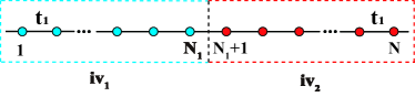
Figure 1: Illustration of the one-dimensional tight binding model with uniform hopping amplitude $t_{1}$ under the periodic boundary condition. The potential $iv_{1}$ is applied to the left $N_{1}$ sites, whereas the potential $iv_{2}$ is applied to the remaining sites.

Figure 2 plots the system’s complex energy spectra and bulk states under the periodic boundary condition. As the imaginary potential goes up, the eigenvalues gradually move along the positive or negative direction of the imaginary axis. Upon reaching a particular imaginary potential, one energy band of the system is divided into two energy bands: an up band $E_{\mathrm{up}}$ with a positive imaginary part and a down band $E_{\mathrm{down}}$ with a negative imaginary part, as shown in Fig.2(c). An imaginary line gap appears between the two energy bands. In particular, there is a $\mathcal{PT}$ transition in which the energy eigenvalues transition from real to complex. Blue circles (red circles) represent the energy eigenvalues moving along the positive (negative) direction of the imaginary axis, whereas black circles represent unmoved energy eigenvalues. The wave functions of moved energy eigenvalues (depicted by the blue curve or the red curve) are bound to the left $N_{1}$ sites or the right $N_{2}$ sites, while the wave functions of unmoved energy eigenvalues (depicted by the black curve) still spread across all sites.

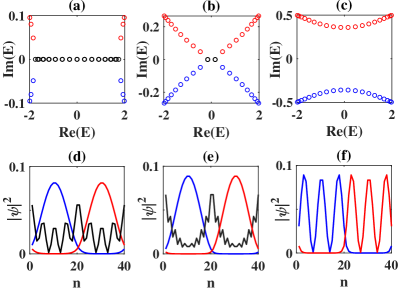
Figure 2: (a), (b) and (c) are complex energy spectra for the imaginary potential strength $v=0.1$, $0.2695$ and $0.5$, respectively. (d), (e) and (f) are their corresponding bulk states versus site $n$. Energy eigenvalues represented by red, black and blue circles correspond to wave functions depicted by red, black and blue curves. Here, $t_{1}=1$ and $N=40$.

The probabilities of an eigenstate $\Psi=\left(\psi_{1},\cdots,\psi_{n}\cdots,\psi_{N}\right)^{{\dagger}}$ of the system in the left $N_{1}$ and right $N_{2}$ sites are

$$\rho_{\mathrm{L}}=\sum_{n=1}^{N_{1}}|\psi_{n}|^{2},\text{ \ \ }\rho_{\mathrm{R}}=\sum_{n=N_{1}+1}^{N}|\psi_{n}|^{2}.$$ (5)

with $\rho_{\mathrm{L}}+\rho_{\mathrm{R}}=1$. Given that the energy eigenvalues move along the imaginary axis, we arrange it in ascending order by imaginary part and show the corresponding probability in Fig.3. It is evident that the probabilities of energy eigenvalues moving along the negative (positive) direction of the imaginary axis are $\rho_{\mathrm{L}}>\rho_{\mathrm{R}}\left(\rho_{\mathrm{L}}<\rho_{\mathrm{R}}\right)$. The left and right probabilities of unmoved energy eigenvalues are equal with $\rho_{\mathrm{L}}=\rho_{\mathrm{R}}=0.5$.

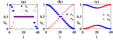
Figure 3: The probability of the one-dimensional tight binding model with uniform hopping. (a), (b) and (c) are the probabilities for the imaginary potential strength $v=0.1$, $0.2695$ and $0.5$, respectively. Here, $t_{1}=1$ and $N=40$.

In order to describe the above phenomena, we give the following concepts:

Theorem-1 — Under the imaginary potential $V=iv_{1}\sum_{n=1}^{N_{1}}c_{n}^{{\dagger}}c_{n}+iv_{2}\sum_{n=N_{1}+1}^{N}c_{n}^{{\dagger}}c_{n}\left(v_{1}<v_{2}\right)$, we arrange the energy eigenvalues of the system in ascending order by imaginary part, $E_{1},\cdots,E_{i},\cdots,E_{N}$. The corresponding eigenstates are $\Psi_{1},\cdots,\Psi_{i},\cdots,\Psi_{N}$, where $i$ is the sort number. In the thermodynamic limit, if

$$\rho_{i,\mathrm{L}}\neq\rho_{i,\mathrm{R}}$$

for all eigenstates, then one energy band of the system can be divided into two energy bands: the down energy band $E_{\mathrm{down}}$ and the up energy band $E_{\mathrm{up}}$. An imaginary line energy gap emerges between these two bands,

$$\Delta=\min\left(\operatorname{Im}E_{\mathrm{up}}\right)-\max\left(\operatorname{Im}E_{\mathrm{down}}\right).$$ (6)

The phenomenon is named “non-Hermitian tearing”.

Theorem-2 — Assuming that there is an eigenstate $\Psi_{i}$, if

$$\rho_{i,\mathrm{L}}=\rho_{i,\mathrm{L}}=0.5,$$

then $\Delta=0$, implying the absence of an imaginary line energy gap. This process is called “partial tearing”. On the contrary, if

$$\rho_{i,\mathrm{L}}\neq\rho_{i,\mathrm{R}}$$

holds true for all eigenstates, then $\Delta>0$, signifying the formation of an imaginary line energy gap. This process is called “complete tearing”.

Definition-1 — The ratio of the probability of an eigenstate $\Psi_{i}$ in the right $N_{2}$ and left $N_{1}$ sites is defined as the tearability of this eigenstate

$$t_{i}=\frac{\rho_{i,\mathrm{R}}}{\rho_{i,\mathrm{L}}}.$$ (7)

Definition-2 — The adjacent part between different imaginary potentials is called the domain wall. The tearing of a state moving perpendicular to the direction of the domain wall is called “separation”. The tearing of a state moving along the direction of the domain wall is called “decoupling”. In particular, we define the direction of the domain wall of a one-dimensional model as the vertical direction.

In Fig.4 (a) and (c), we calculate the tearability $t$ of the $i=11$ and the $i=31$ bulk states, respectively. The tearability $t=1$ indicates that the bulk state is in the phase with $\mathcal{PT}$ symmetry and the tearability $t\rightarrow 0$ $\left(i=11\right)$ or $t\rightarrow\infty$ $\left(i=31\right)$ indicates that the bulk state is in the phase with $\mathcal{PT}$-symmetry breaking. They are continuous at the exceptional point where their energy eigenvalues transition from real to complex numbers. Furthermore, we calculate their derivatives $\frac{\partial t}{\partial v}$ in Fig.4 (b) and (d). $\frac{\partial t}{\partial v}$ is discontinued at the exceptional point, which means a second-order phase transition at the exceptional point.

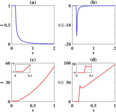
Figure 4: (a) and (b) are the tearability $t$ and the derivative $\frac{\partial t}{\partial v}$ of the $i=11$ bulk state, respectively. (c) and (d) are the tearability $t$ and derivative $\frac{\partial t}{\partial v}$ of the $i=31$ bulk state, respectively. Here, $t_{1}=1$ and $N=40$.

To better understand non-Hermitian tearing, we give an effective $2\times 2$ Hamiltonian $H_{\mathrm{eff}}$ in the $k$-space, obtained from reducing the $N\times N$ Hamiltonian $H=H_{0}+V$ in the real space, which can explain the imaginary line gap and the $\mathcal{PT}$ transition.

Theorem-3: The effective $2\times 2$ Hamiltonian $H_{\mathrm{eff}}$ can be written as $H_{\mathrm{eff}}=\sum_{k}\left(\begin{array}[c]{cc}a_{k}^{{\dagger}}&b_{k}^{{\dagger}}\end{array}\right)h_{\mathrm{eff}}\left(k\right)\left(\begin{array}[c]{c}a_{k}\\ b_{k}\end{array}\right)$, where

$$h_{\mathrm{eff}}\left(k\right)=\left(\begin{array}[c]{cc}h_{0}-ivI&\alpha\\ \alpha&h_{0}+ivI\end{array}\right)$$ (8)

with the Bloch Hamiltonian $h_{0}$ of $H_{0}$ and the coupling term $\alpha$ between the left $N_{1}$ and right $N_{2}$ sites. Here, $k=\frac{2\pi}{N_{1}}i,i=1,2,\cdots,N_{1}$ and $I$ is the identity matrix. The eigenvalues are

$$E_{\mathrm{eff}}\left(k\right)=E_{0}\pm\frac{\Delta}{2},$$ (9)

where $E_{0}$ is eigenvalue of $H_{0}$. When $\Delta$ is real, the eigenstate of the system is in the phase with $\mathcal{PT}$-symmetry; when $\Delta$ is complex, the eigenstate of the system is in the phase with $\mathcal{PT}$-symmetry breaking.

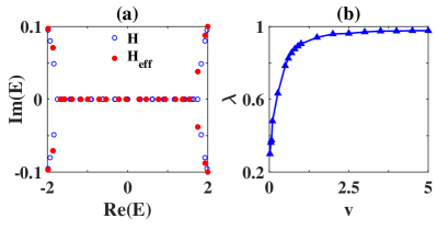
Figure 5: (a) The complex energy spectra from numerical solutions of the Hamiltonian $H$ in the real space and the analytical solutions of the effective Hamiltonian $H_{\mathrm{eff}}$ in the $k$-space, where $v=0.1$ and $\lambda=0.493$. (b) The fitting parameter $\lambda$ versus the imaginary potential strength $v$. Here, $t_{1}=1$ and $N=40$.

For the simple one-dimensional tight binding model with uniform hopping under the imaginary potential, $h_{\mathrm{eff}}\left(k\right)$ is expressed as

$$h_{\mathrm{eff}}\left(k\right)=\left(\begin{array}[c]{cc}E_{0}-iv&\alpha\\ \alpha&E_{0}+iv\end{array}\right),$$ (10)

where $\alpha=\frac{2t\sin k}{\sqrt{N_{1}}}\cdot\lambda$ and $\lambda$ is a fitting parameter related to $v$. The eigenvalues are

$$E_{\mathrm{eff}}=E_{0}\pm\sqrt{\alpha^{2}-v^{2}}.$$ (11)

The complex energy spectra from numerical solutions of the Hamiltonian $H$ in the real space and the analytical solutions of the effective Hamiltonian $H_{\mathrm{eff}}$ in the $k$-space fit well, as shown in Fig.5(a). For a given $k$, if $\alpha^{2}-v^{2}>0$, then $E_{\mathrm{eff}}$ is a real number and this corresponding bulk state is in partial tearing. As $v^{2}>>\alpha^{2}$ for all $k$, then $E_{\mathrm{eff}}$ is a complex number and all bulk states is in complete tearing. The imaginary line gap is

$$\Delta=2\sqrt{\alpha^{2}-v^{2}}.$$ (12)

As $\alpha^{2}-v^{2}=0$, that is,

$$k=k_{0}=\pm\arcsin\frac{v\sqrt{N_{1}}}{2t\lambda},$$ (13)

then $E_{\mathrm{eff}}\left(k_{0}\right)=E_{0}\left(k_{0}\right)$ and the bulk state is at the $\mathcal{PT}$ transition. Because bulk states move perpendicular to the direction of the domain wall, bulk states show separation. See the detailed calculations regarding the probability and tearability of eigenstates of $H_{\mathrm{eff}}$ in Appendix A. Besides, we also give the fitting parameter $\lambda$ as a function of $v$ in Fig.5(b). $\lambda$ reaches a saturation value $1$ when $v$ is increased to a large value.

Given a more general case, a complex potential for the system is

$$V =v_{1}e^{i\phi_{1}}\sum_{i=1}^{N_{1}}c_{i}^{{\dagger}}c_{i}+v_{2}e^{i\phi_{2}}\sum_{i=N_{1}+1}^{N_{1}+N_{2}}c_{i}^{{\dagger}}c_{i}$$

$$+\cdots+v_{n}e^{i\phi_{n}}\sum_{i=N_{n-1}+1}^{N_{1}+\cdots+N_{n}}c_{i}^{{\dagger}}c_{i},$$ (14)

where the real number $v_{1,2,\cdots,n}$ represents the magnitudes of the $n$ uniform complex potentials and $\phi_{1,2,\cdots,n}$ is their phase angle with $\phi_{1,2,\cdots,n}\in\left[0,2\pi\right]$. Here, $N=N_{1}+N_{2}+\cdots+N_{n}$. In the system, the uniform complex potential $v_{1}e^{i\phi_{1}}$ is applied to the $N_{1}$ sites, the uniform complex potential $v_{2}e^{i\phi_{2}}$ is applied to the $N_{2}$ sites, and so on. Using a two-dimensional square lattice model as an example, we consider the complex potential in Fig.6(a). The energy spectra of the system are torn to different positions along different directions, depending on the form of the uniform complex potential, as illustrated in Fig.6(b). The direction is the phase angle of the uniform complex potential, and the position is relevant to the amplitude of the uniform complex potential, as shown in Fig.6(b).

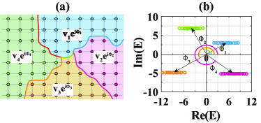
Figure 6: The two-dimensional square lattice model with uniform hopping under the periodic boundary conditions along the x-direction and y-direction. The four different uniform complex potentials are $v_{1}e^{i\phi_{1}}$, $v_{2}e^{i\phi_{2}}$, $v_{3}e^{i\phi_{3}}$, and $v_{4}e^{i\phi_{4}}$, respectively. (a) The model diagram. (b) The energy spectrum. Here, $v_{1}=6$, $v_{2}=8$, $v_{3}=10$, $v_{4}=9$, and $\phi_{1}=\frac{\pi}{6}$, $\phi_{2}=\frac{2\pi}{3}$, $\phi_{3}=\frac{7\pi}{6}$, $\phi_{4}=\frac{9\pi}{5}$.

III Non-Hermitian tearing in one-dimensional SSH model

In this section, we consider the one-dimensional tight binding model with non-uniform hopping. Here, we take the one-dimensional SSH model as an example, which its Hamiltonian is

$$H_{\mathrm{SSH}}=t_{1}\sum_{n=1}^{N}|n,B\rangle\langle n,A|+t_{2}\sum_{n=1}^{N-1}|n+1,A\rangle\langle n,B|+h.c.,$$ (15)

where $A$ and $B$ denote the two sublattices of each pair of lattice sites. $t_{1}$ and $t_{2}$ describe the intra-cell and inter-cell hopping strengths, respectively. Here, we set $t_{2}=2t_{1}=2$. The Bloch Hamiltonian of this model is

$$H_{\mathrm{SSH}}\left(k\right)=\left(t_{1}+t_{2}\cos k\right)\sigma_{x}+\left(t_{2}\sin k\right)\sigma_{y},$$ (16)

where $\sigma_{i}$’s are the Pauli matrices acting on the sublattice subspace. Its eigenvalue in the $k$-space is

$$E_{\pm}\left(k\right)=\pm\sqrt{\left(t_{1}+t_{2}\cos k\right)^{2}+\left(t_{2}\sin k\right)^{2}}.$$ (17)

Here, we consider the imaginary potential for the one-dimensional SSH model, as shown in Fig.7.

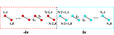
Figure 7: The one-dimensional Su-Schrieffer-Heeger model under the periodic boundary condition. $t_{1}$ and $t_{2}$ describe the intra-cell and inter-cell hopping strengths, respectively. The $N$ pairs of lattice sites are divided equally into two parts, which the left $N/2$ pairs of lattice sites are subject to the potential $-iv$, and the remaining $N/2$ pairs of lattice sites are subject to the potential $iv$.

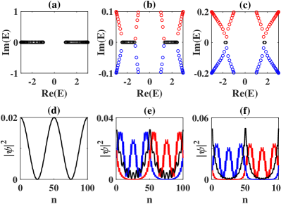
Figure 8: (a), (b) and (c) are the complex energy spectra for the imaginary potential strength $v=0,0.1$ and $0.2$, respectively. (d) to (f) are their corresponding bulk states versus site $n$. Energy eigenvalues represented by red, black and blue circles correspond to wave functions depicted by red, black and blue curves. Here, $t_{1}=1,t_{2}=2,$ and $N=50$.

We show the complex energy spectra and eigenstates of the system under the periodic boundary condition in Fig.8 and Fig.9. The one-dimensional SSH model also exhibits non-Hermitian tearing, accompanied by a $\mathcal{PT}$ transition and the separation of bulk states. However, after bulk states are torn apart, two pairs of boundary states emerge, as depicted in Fig.9. As the imaginary potential strength $v$ continues to increase, these two pairs of boundary states also show non-Hermitian tearing along with a $\mathcal{PT}$ transition. As a result, the wave function of the boundary state, depicted by the blue curve with asterisks corresponding to the down energy band (represented by blue asterisks), is localized on the two boundaries of the left $N/2$ pairs of lattice sites. On the contrary, the wave function of the boundary state, depicted by the red curve with red plus signs corresponding to the up energy band (represented by red plus signs), is localized on the two boundaries of the right $N/2$ pairs of lattice sites in Fig.9(f). Since these boundary states move along the direction of the domain wall, their tearing manifests as decoupling.

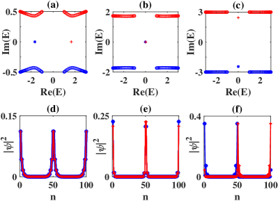
Figure 9: (a), (b) and (c) are the complex energy spectra for the imaginary potential strength $v=0.5,1.732$ and $3$, respectively. (d), (e) and (f) are one of the left (depicted by blue curve with asterisks) and right (depicted by red curve with plus sign) boundary states, respectively. Here, $t_{1}=1,t_{2}=2,$ and $N=50$.

To better analyse the tearing of boundary states, we calculate the tearability $t$ for the $i=1$ and the $i=4$ boundary states in Fig.10 (a) and (c), respectively. $t=1$ indicates that the boundary state is in the phase with $\mathcal{PT}$-symmetry, whereas $t\rightarrow 0$ $\left(i=1\right)$ or $t\rightarrow\infty$ $\left(i=4\right)$ indicates that the boundary state is in the phase with $\mathcal{PT}$-symmetry breaking. They are continuous at the exceptional point where their energy eigenvalues transition from real to imaginary numbers. Their derivatives $\frac{\partial t}{\partial v}$ are displayed in Fig.10 (b) and (d). At the exceptional point, $\frac{\partial t}{\partial v}$ is discontinued, which implies a second-order phase transition at the exceptional point.

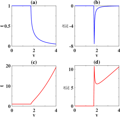
Figure 10: (a) and (b) are the tearability $t$ and the derivative $\frac{\partial t}{\partial v}$ of the $i=1$ boundary state, respectively. (c) and (d) are the tearability $t$ and the derivative $\frac{\partial t}{\partial v}$ of the $i=4$ boundary state, respectively. Here, $t_{1}=1$ and $N=40$.

According to Theorem-3, we give the effective Hamiltonian of one-dimensional SSH model subject to the imaginary potential under the periodic boundary condition to understand its non-Hermitian tearing for the bulk states and boundary states. Firstly, the effective Hamiltonian of bulk states is written as

$$h_{\mathrm{eff}}=\left(\begin{array}[c]{cc}h_{11}&h_{12}\\ h_{21}&h_{22}\end{array}\right)$$ (18)

with

$$h_{11} =\left(\begin{array}[c]{cc}-iv&t_{1}+t_{2}e^{-ik}\\ t_{1}+t_{2}e^{ik}&-iv\end{array}\right),$$ (21)

$$h_{12} =h_{21}=i\frac{\lambda}{\sqrt{N_{1}}}\left(\begin{array}[c]{cc}0&t_{1}+t_{2}e^{-i\left(k+\pi\right)}\\ -\left[t_{1}+t_{2}e^{i\left(k+\pi\right)}\right]&0\end{array}\right),$$ (24)

$$h_{22} =\left(\begin{array}[c]{cc}iv&t_{1}+t_{2}e^{-ik}\\ t_{1}+t_{2}e^{ik}&iv\end{array}\right).$$ (27)

Here, $k=\frac{2\pi}{N_{1}}i,i=1,2,\cdots,N_{1}$. These solutions from the Hamiltonian $H=H_{\mathrm{SSH}}+V$ in the real space and the effective Hamiltonian $H_{\mathrm{eff}}$ in the $k$-space for bulk states fit well in Fig.11.

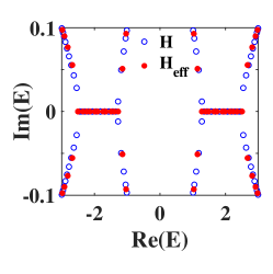
Figure 11: The complex energy spectra from numerical solutions of the Hamiltonian $H$ in the real space and the analytical solutions of the effective Hamiltonian $H_{\mathrm{eff}}$ in the $k$-space, respectively, where $v=0.1$ and $\lambda=0.392$. Here, $t_{1}=1,t_{2}=2,$ and $N=50$.

Secondly, the effective Hamiltonian of boundary states is given by $h_{\mathrm{eff}}=I\otimes h$, where

$$h=iv\sigma_{z}+\sqrt{3}\sigma_{y},$$ (28)

and $I=\left(\begin{array}[c]{cc}1&0\\ 0&1\end{array}\right)$. The eigenvalue is

$$E_{\mathrm{eff}}=\pm\sqrt{3-v^{2}},$$ (29)

The solutions of the effective Hamiltonian $H_{\mathrm{eff}}$ in the $k$-space for boundary states agree with those of the Hamiltonian $H=H_{\mathrm{SSH}}+V$ in the real space in Fig.12. There is a $\mathcal{PT}$ transition: in the case of $v<\sqrt{3}$, the eigenvalues are all real and boundary states are at $\mathcal{PT}$ -symmetry; and in the case of $v>\sqrt{3}$, the eigenvalues are all imaginary and boundary states are at $\mathcal{PT}$ -broken. At $v=\sqrt{3}$, boundary states are at the exceptional point with energy degeneracy, i.e., $E_{\mathrm{eff}}\left(k\right)=0$.

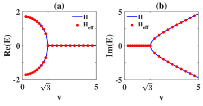
Figure 12: The numerical solutions of boundary states from the Hamiltonian $H$ in the real space and the analytical solutions of the effective Hamiltonian $H_{\mathrm{eff}}$ in the $k$-space, respectively. Here, $t_{1}=1,t_{2}=2,$ and $N=50$.

IV Non-Hermitian tearing in the QWZ model

In the section, we take the QWZ model as an example and discuss the non-Hermitian tearing in the two-dimensional model. The Hamiltonian of the QWZ model in the real space is

$$H_{\mathrm{QWZ}} =\sum_{m_{x}=1}^{N_{x}-1}\sum_{m_{y}=1}^{N_{y}}\left(|m_{x}+1,m_{y}\rangle\langle m_{x},m_{y}|\otimes t_{x}+h.c.\right)$$

$$+\sum_{m_{x}=1}^{N_{x}}\sum_{m_{y}=1}^{N_{y}-1}\left(|m_{x},m_{y}+1\rangle\langle m_{x},m_{y}|\otimes t_{y}+h.c.\right)$$

$$+u\sum_{m_{x}=1}^{N_{x}}\sum_{m_{y}=1}^{N_{y}}|m_{x},m_{y}\rangle\langle m_{x},m_{y}|\otimes\sigma_{z},$$ (30)

where $u$ is the staggered on site potential. The model describes a particle with two internal states hopping on a lattice where the nearest neighbour hopping is accompanied by an operation on the internal degree of freedom, and this operation is different for the hopping along the x with $t_{x}=\frac{\sigma_{z}+i\sigma_{x}}{2}$ and y directions with $t_{y}=\frac{\sigma_{z}+i\sigma_{y}}{2}$. The Bloch Hamiltonian in the $k$-space is given by

$$H_{\mathrm{QWZ}}\left(k\right)=\sin k_{x}\cdot\sigma_{x}+\sin k_{y}\cdot\sigma_{y}+\left(\cos k_{x}+\cos k_{y}+u\right)\cdot\sigma_{z},$$ (31)

and its eigenvalue is

$$E_{\pm}\left(k\right)=\pm\sqrt{\left(\sin k_{x}\right)^{2}+\left(\sin k_{y}\right)^{2}+\left(\cos k_{x}+\cos k_{y}+u\right)^{2}}.$$ (32)

The imaginary potential is

$$V =-iv\sum_{m_{x}=1}^{L/2}\sum_{m_{y}=1}^{N/2}|m_{x},m_{y}\rangle\langle m_{x},m_{y}|\otimes I$$

$$+iv\sum_{m_{x}=L/2+1}^{L}\sum_{m_{y}=N/2+1}^{N}|m_{x},m_{y}\rangle\langle m_{x},m_{y}|\otimes I.$$ (33)

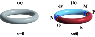
Figure 13: The diagram of the Qi-Wu-Zhang model under the periodic conditions along the x-direction and y-direction. (a) represents the case without imaginary potential. (b) represents the case with imaginary potential. M, N, O, and P denote two sides of two domain walls, respectively. The arrow represents the chiral direction.

We first discuss the case of the periodic boundary both along the x-direction and the y-direction, as plotted in Fig.13. The complex energy spectra and eigenstates of the model are shown in Fig.14 and Fig.15. Obviously, bulk states have a $\mathcal{PT}$ transition and separation. After the separation of bulk states, the system appears a number of boundary states in Fig.15. Each energy eigenvalue of the boundary state has two eigenstates. Therefore, here we only take one of the eigenstates in Fig.15.

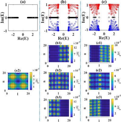
Figure 14: The Qi-Wu-Zhang model under the periodic conditions both along the x-direction and y-direction. (a), (b) and (c) are the complex energy spectra for the imaginary potential strength $v=0$, $0.1$ and $0.21$, respectively. (a2) is a bulk state versus the site $n$ and $l$ for $v=0$. (b1)-(b3) are bulk states versus the site $n$ and $l$ corresponding to the energy eigenvalues represented by the red, black, and blue circles for $v=0.1$, respectively. (c1)-(c3) are bulk states versus the site $n$ and $l$ corresponding to the energy eigenvalues represented by the red, black, and blue circles for $v=0.21$, respectively. Here, $N=L=20$ and $u=-1$.

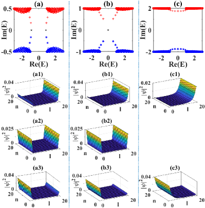
Figure 15: The Qi-Wu-Zhang model under the periodic conditions both along the x-direction and y-direction. (a), (b) and (c) are the complex energy spectra for the imaginary potential strength $v=0.5$, $1$ and $2$, respectively. (a1)-(a3) are boundary states versus the site $n$ and $l$ corresponding to the energy eigenvalues represented by the red plus signs, black crosses, and blue asterisks for $v=0.5$, respectively. (b1)-(b3) are boundary states versus the site $n$ and $l$ corresponding to the energy eigenvalues represented by the red plus signs, black crosses, and blue asterisks for $v=1$, respectively. (c1) and (c3) are boundary states versus the site $n$ and $l$ corresponding to the energy eigenvalues represented by the red plus signs and blue asterisks for $v=2$, respectively. Here, $N=L=20$ and $u=-1$.

With the increase of the imaginary potential strength $v$, these boundary states show non-Hermitian tearing with a $\mathcal{PT}$ transition. As a consequence, the wave functions of boundary states, corresponding the down energy band with a negative imaginary part (represented by blue asterisks), are only localized at the position M or N, in Fig13.(b). The wave functions of boundary states, corresponding the up energy band with a positive imaginary part (represented by red plus signs), are only localized at the position O or P, in Fig13.(b). The chiral direction of boundary states is along the direction of domain walls, thus boundary states appear decoupling. Moreover, we plot the probabilities $\rho_{\mathrm{L},\mathrm{R}}$ of boundary states in Fig.16. The probabilities of the coupled boundary states are $\rho_{\mathrm{L}}=\rho_{\mathrm{R}}=0.5$, whereas the probabilities of decoupled boundary states are $\rho_{\mathrm{L}}\neq\rho_{\mathrm{R}}$. We calculate the tearability and its derivative of the $i=350$ and the $i=450$ eigenstates in Fig.17. There is a second-order phase transition about the tearability at the exceptional point.

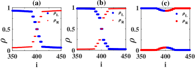
Figure 16: The probabilities of the Qi-Wu-Zhang model under the periodic conditions both along the x-direction and y-direction. (a), (b) and (c) are the probabilities for the imaginary potential strength $v=0.5$, $1$ and $2$, respectively. Here, $N=L=20$ and $u=-1$.

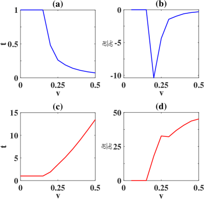
Figure 17: The tearability $t$ and the derivative $\frac{\partial t}{\partial v}$ of the Qi-Wu-Zhang model under the periodic conditions both along the x-direction and y-direction. (a) and (b) are $t$ and $\frac{\partial t}{\partial v}$ of the $i=350$ eigenstate, respectively. (c) and (d) are $t$ and $\frac{\partial t}{\partial v}$ of the $i=450$ eigenstate, respectively. Here, $N=L=20$ and $u=-1$.

We provide the effective Hamiltonian for this situation. The effective Hamiltonian of bulk states is

$$h_{\mathrm{eff}}=\left(\begin{array}[c]{cc}h_{11}&h_{12}\\ h_{21}&h_{22}\end{array}\right),$$ (34)

where

$$h_{11} =H_{\mathrm{QWZ}}\left(k\right)-ivI,$$

$$h_{12} =h_{21}=\frac{\lambda_{1}}{\sqrt{L_{1}}}\left[\sin\left(k_{x}+\pi\right)\cdot\sigma_{x}+\cos\left(k_{x}+\frac{\pi}{2}\right)\cdot\sigma_{z}\right],$$

$$h_{22} =H_{\mathrm{QWZ}}\left(k\right)+ivI.$$ (35)

$\lambda_{1}$ is the fitting parameter. Here, $k=\frac{2\pi}{L_{1}}i,i=1,2,\cdots,L_{1}$ and $L_{1}=L/2$. For the boundary states, the effective Hamiltonian is

$$h_{\mathrm{eff}}=\left(\begin{array}[c]{cc}-\sin k_{x}-iv&\frac{\lambda_{2}}{\sqrt{L_{1}}}\\ \frac{\lambda_{2}}{\sqrt{L_{1}}}&\sin k_{x}+iv\end{array}\right),$$ (36)

where $\lambda_{2}$ is the fitting parameter. The numerical solutions of the Hamiltonian $H=H_{\mathrm{SSH}}+V$ (blue circles) in the real space and the analytical solutions of the effective Hamiltonian $H_{\mathrm{eff}}$ (red dots) in the $k$-space for bulk states and boundary states are shown in Fig.18.

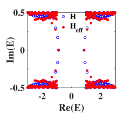
Figure 18: The complex energy spectra from numerical solutions of the Hamiltonian $H$ in the real space and the analytical solutions of the effective Hamiltonian $H_{\mathrm{eff}}$ in the $k$-space, where $v=0.5$ $\lambda_{1}=0.75$ and $\lambda_{2}=3.162$.

Furthermore, we study the case of the periodic boundary condition along the x-direction and the open boundary condition along the y-direction, as shown in Fig.19. In the absence of imaginary potential, the system exhibits a series of intrinsic boundary states that are localized on one side of the y-direction boundary (at the position Q or R). Here, we only provide the wave function of one of the intrinsic boundary states in Fig.20(a2). Obviously, there are also the $\mathcal{PT}$ transition and the separation of bulk states in Fig.20.

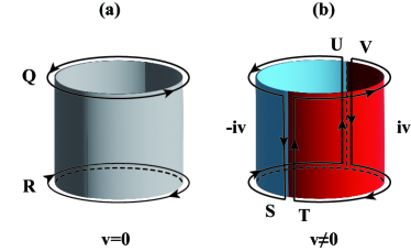
Figure 19: The diagram of the Qi-Wu-Zhang model under the periodic boundary condition along the x-direction and the open boundary condition along the y-direction. (a) represents the case without imaginary potential. Q and R denote two sides of the y-direction boundary, respectively. (b) represents the case with imaginary potential. M, N, O, and P denote two points of two domain walls. The arrow represents the chiral direction.

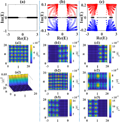
Figure 20: The Qi-Wu-Zhang model under the periodic boundary condition along the x-direction and the open boundary condition along the y-direction. (a), (b) and (c) are the complex energy spectra for the imaginary potential strength $v=0$, $0.1$ and $0.21$, respectively. (a1) and (a2) are a bulk state and a topological boundary state versus the site $n$ and $l$ corresponding to the energy eigenvalues represented by the black circles and black crosses for $v=0$, respectively. (b1)-(b3) are bulk states versus the site $n$ and $l$ corresponding to the energy eigenvalues represented by the red, black, and blue circles for $v=0.1$, respectively. (c1)-(c3) are bulk states versus the site $n$ and $l$ corresponding to the energy eigenvalues represented by the red, black, and blue circles for $v=0.21$, respectively. $N=L=20$ and $u=-1$.

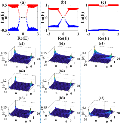
Figure 21: The Qi-Wu-Zhang model under the periodic boundary condition along the x-direction and the open boundary condition along the y-direction. (a), (b) and (c) are the complex energy spectra for the imaginary potential strength $v=0.5$, $0.7135$ and $2$, respectively. (a1)-(a3) are boundary states versus the site $n$ and $l$ corresponding to the energy eigenvalues represented by the red plus signs, black crosses and blue asterisks for $v=0.5$, respectively. (b1)-(b3) are boundary states versus the site $n$ and $l$ corresponding to the energy eigenvalues represented by the red plus signs, black crosses and blue asterisks for $v=0.7135$, respectively. (c1) and (c3) are bulk states versus the site $n$ and $l$ corresponding to the energy eigenvalues represented by the red plus signs and blue asterisks for $v=2$, respectively. Here, $N=L=20$ and $u=-1$.

As the imaginary potential increases, new boundary states (represented by blue asterisks or red plus signs) appear and form a $\mathcal{PT}$ transition with intrinsic boundary states (represented by black crosses) in Fig.21. The wave function of the intrinsic boundary state, corresponding the energy band with zero imaginary part (represented by black crosses), is equally located on the points S and T or the points U and V due to chiral skin effect, as shown in Fig.21(a2) and (b2) X2023 . Due to the unequal imaginary potentials of $-iv$ and $iv$ at the two domain walls, the wave function at both sides of the two domain walls tends to localize at the points T and V in Fig21.(a1) or the points S and U in Fig.21(a3). In this process, intrinsic boundary states and the wave function at both sides of the two domain walls occur reconstruction. After the $\mathcal{PT}$ transition of boundary states, these boundary states show decoupling in Fig.21(c). The wave function of the boundary state, corresponding the down energy band with negative imaginary part (blue asterisks), is only distributed at the points S and U, in Fig21.(c3). The wave function of the boundary state, corresponding the up energy band with positive imaginary part (red plus signs), is only distributed at the points T and V, in Fig21.(c1).

V Conclusions

In the paper, we study the non-Hermitian system under dissipation, where the left and right sites are subject to different imaginary potentials. We find that the energy band shows an imaginary line gap and energy eigenstates are bound to a specific region. For these phenomena, we propose the non-Hermitian tearing theory, in which the system is either in partial tearing or complete tearing, accompanied by a $\mathcal{PT}$ transition. The ‘tearability’ we define exhibits a continuous phase transition at the exceptional point. During the non-Hermitian tearing, the system has the following properties: (1) bulk states show separation; (2) in a topological system, there is the emergence and decoupling of boundary states; (3) with nonreciprocal hopping, bulk states will display skin effect in the bound region, which will be our subsequent study. To better understand the non-Hermitian tearing, we provide the effective $2\times 2$ Hamiltonian in the $k$-space for both bulk and boundary states by reducing the $N\times N$ Hamiltonian in the real space. In particular, boundary states undergo reconstruction in the QWZ model under the periodic boundary condition along the x-direction and open boundary condition along the y-direction. In the future, we will study the interplay of non-Hermitian tearing with other effects, such as the skin effect, to discover more novel phenomena and mechanisms.

Appendix A The probability and tearability of eigenstates of the effective Hamiltonian

For the simple one-dimensional tight binding model with uniform hopping under the imaginary potential, $h_{\mathrm{eff}}\left(k\right)$ is expressed as

$$h_{\mathrm{eff}}\left(k\right)=\left(\begin{array}[c]{cc}E_{0}-iv&\alpha\\ \alpha&E_{0}+iv\end{array}\right),$$ (37)

where $\alpha=\frac{2t\sin k}{\sqrt{N_{1}}}\cdot\lambda$ and $\lambda$ is a fitting parameter related to $v$. The eigenvalues are

$$E_{\mathrm{eff}}=E_{0}\pm\sqrt{\alpha^{2}-v^{2}}.$$ (38)

The eigenstates are

$$\Psi_{+}=\frac{1}{A}\binom{1}{\frac{iv+\sqrt{\alpha^{2}-v^{2}}}{\alpha}},\Psi_{-}=\frac{1}{B}\binom{1}{\frac{iv-\sqrt{\alpha^{2}-v^{2}}}{\alpha}},$$ (39)

where $A=\sqrt{1+\left(\frac{iv+\sqrt{\alpha^{2}-v^{2}}}{\alpha}\right)^{2}}$ and $B=\sqrt{1+\left(\frac{iv-\sqrt{\alpha^{2}-v^{2}}}{\alpha}\right)^{2}}$. The corresponding probabilities are

$$\rho_{+,\mathrm{L}} =\frac{\alpha^{2}}{\alpha^{2}+\left(iv+\sqrt{\alpha^{2}-v^{2}}\right)^{2}},$$

$$\rho_{+,\mathrm{R}} =\frac{\left(iv+\sqrt{\alpha^{2}-v^{2}}\right)^{2}}{\alpha^{2}+\left(iv+\sqrt{\alpha^{2}-v^{2}}\right)^{2}},$$

$$\rho_{-,\mathrm{L}} =\frac{\alpha^{2}}{\alpha^{2}+\left(iv-\sqrt{\alpha^{2}-v^{2}}\right)^{2}},$$

$$\rho_{-,\mathrm{R}} =\frac{\left(iv-\sqrt{\alpha^{2}-v^{2}}\right)^{2}}{\alpha^{2}+\left(iv-\sqrt{\alpha^{2}-v^{2}}\right)^{2}}.$$ (40)

The tearability are

$$t_{+} =\frac{\left(iv+\sqrt{\alpha^{2}-v^{2}}\right)^{2}}{\alpha^{2}},$$

$$t_{-} =\frac{\left(iv-\sqrt{\alpha^{2}-v^{2}}\right)^{2}}{\alpha^{2}}.$$ (41)

References

- (1) C. E. Rüer, K. G. Makris, R. El-Ganainy, D. N. Christodoulides, M. Segev, and D. Kip, Observation of parity–time symmetry in optics, Nat. Phys. 6, 192 (2010).
- (2) A. Guo, G. J. Salamo, D. Duchesne, R. Morandotti, M. Volatier-Ravat, V. Aimez, G. A. Siviloglou, and D. N. Christodoulides, Observation of -Symmetry Breaking in Complex Optical Potentials Phys. Rev. Lett. 103, 093902 (2009).
- (3) Y. D. Chong, L. Ge, and A. D. Stone, -Symmetry Breaking and Laser-Absorber Modes in Optical Scattering Systems, Phys. Rev. Lett. 106, 093902 (2011).
- (4) R. El-Ganainy, K. G. Makris, M. Khajavikhan, Z. H. Musslimani, S. Rotter, and D. N. Christodoulides, Non-Hermitian physics and PT symmetry, Nat. Phys. 14, 11 (2018).
- (5) L. Feng, Y.-L. Xu, W. S. Fegadolli, M.-H. Lu, J. E. B. Oliveira, V. R. Almeida, Y.-F. Chen, and A. Scherer, Experimental demonstration of a unidirectional reflectionless parity-time metamaterial at optical frequencies, Nat. Mater. 12, 108 (2013).
- (6) H. Hodaei, M.-A. Miri, M. Heinrich, D. N. Christodoulides, and M. Khajavikhan, Parity-time-symmetric microring lasers, Science 346, 975 (2014).
- (7) L. Feng, Z. J. Wong, R.-M. Ma, Y. Wang, and X. Zhang, Single mode laser by parity-time symmetry breaking, Science 346, 972 (2014).
- (8) W. Song, W. Sun, C. Chen, Q. Song, S. Xiao, S. Zhu, and T. Li, Breakup and Recovery of Topological Zero Modes in Finite Non-Hermitian Optical Lattices, Phys. Rev. Lett. 123, 165701 (2019).
- (9) V. Kozii and L. Fu, Non-Hermitian Topological Theory of Finite-Lifetime Quasiparticles: Prediction of Bulk Fermi Arc due to Exceptional Point, arXiv:1708.05841.
- (10) Z. Gong, Y. Ashida, K. Kawabata, K. Takasan, S. Higashikawa, and M. Ueda, Topological Phases of Non Hermitian Systems, Phys. Rev. X 8, 031079 (2018).
- (11) H. Shen, B. Zhen, and L. Fu, Topological Band Theory for Non-Hermitian Hamiltonians, Phys. Rev. Lett. 120, 146402 (2018).
- (12) F. Song, S. Yao, and Z. Wang, Non-Hermitian Topological Invariants in Real Space, Phys. Rev. Lett. 123, 246801 (2019).
- (13) N. Matsumoto, K. Kawabata, Y. Ashida, S. Furukawa, and M. Ueda, Continuous Phase Transition without Gap Closing in Non-Hermitian Quantum Many-Body Systems, Phys. Rev. Lett. 125, 260601 (2020).
- (14) K. Kawabata, K. Shiozaki, M. Ueda, and M. Sato, Symmetry and Topology in Non-Hermitian Physics, Phys. Rev. X 9, 041015 (2019).
- (15) K. Kawabata, K. Shiozaki, and S. Ryu, Topological Field Theory of Non-Hermitian Systems, Phys. Rev. Lett. 126, 216405 (2021).
- (16) Y. Michishita and R. Peters, Equivalence of Effective Non-Hermitian Hamiltonians in the Context of Open Quantum Systems and Strongly Correlated Electron Systems, Phys. Rev. Lett. 124, 196401 (2020).
- (17) C. M. Bender, D. C. Brody, and H. F. Jones, Complex Extension of Quantum Mechanics, Phys. Rev. Lett. 89, 270401 (2002).
- (18) I. Rotter, A non-Hermitian Hamilton operator and the physics of open quantum systems, J. Phys. A: Math. Theor. 42, 153001 (2009).
- (19) F. Reiter and A. S. Sørensen, Effective operator formalism for open quantum systems, Phys. Rev. A 85, 032111 (2012).
- (20) A. Mostafazadeh, Pseudo-Hermiticity versus PT symmetry: The necessary condition for the reality of the spectrum of a non-Hermitian Hamiltonian J. Math. Phys. 43 205 (2002); A. Mostafazadeh, Pseudo-Hermiticity versus PT-symmetry. II. A complete characterization of non-Hermitian Hamiltonians with a real spectrum, ibid, 43 2814 (2002); A. Mostafazadeh A, Pseudo-Hermiticity versus PT-symmetry III: Equivalence of pseudo-Hermiticity and the presence of antilinear symmetries, ibid, 43 3944, (2002).
- (21) N. Moiseyev, Non-Hermitian Quantum Mechanics (Cambridge University Press, Cambridge, 2011).
- (22) Y. Ashida, Z. Gong, and M. Ueda, Non-Hermitian physics, Adv. Phys. 69, 249 (2020).
- (23) C. M. Bender, Making sense of non-Hermitian Hamiltonians, Rep. Prog. Phys. 70, 947 (2007).
- (24) G. Gamow, Zur Quantentheorie des Atomkernes, Z. Phys. 51, 204 (1928).
- (25) P. M. Radmore and P. L. Knight, Population trapping and dispersion in a three-level system, J. Phys. B: Atom. Mol. Phys., 15, 561 (1982).
- (26) R. M. More, Theory of decaying states, Phys. Rev. A 4, 1782 (1971).
- (27) N. Hatano and D. R. Nelson, Localization Transitions in Non-Hermitian Quantum Mechanics, Phys. Rev. Lett. 77, 570 (1996).
- (28) C. M. Bender, and S. Boettcher, Phys. Rev. Lett. 80, 5243 (1998).
- (29) V. M. Martinez Alvarez, J. E. Barrios Vargas, and L. E. F. Foa Torres, Non-Hermitian robust edge states in one dimension: Anomalous localization and eigenspace condensation at exceptional points, Phys. Rev. B 97, 121401(R) (2018).
- (30) S. Yao and Z. Wang, Edge States and Topological Invariants of Non-Hermitian Systems, Phys. Rev. Lett. 121, 086803 (2018).
- (31) L. Li, C. H. Lee, S. Mu, and J. Gong, Critical non-Hermitian skin effect, Nat. Commun. 11, 5491 (2020).
- (32) K. Kawabata, M. Sato, and K. Shiozaki, Higher-order non-hermitian skin effect, Phys. Rev. B 102, 205118 (2020).
- (33) D. S. Borgnia, A. J. Kruchkov, and R.-J. Slager, Non-Hermitian Boundary Modes and Topology, Phys. Rev. Lett. 124, 056802 (2020).
- (34) N. Okuma, K. Kawabata, K. Shiozaki, and M. Sato, Topological Origin of Non-Hermitian Skin Effects, Phys. Rev. Lett. 124, 086801 (2020).
- (35) Y. Xiong, Why does bulk boundary correspondence fail in some non-hermitian topological models, J. Phys. Commun. 2 035043 (2018).
- (36) T. E. Lee, Anomalous Edge State in a Non-Hermitian Lattice, Phys. Rev. Lett. 116, 133903 (2016).
- (37) F. K. Kunst, E. Edvardsson, J. C. Budich, and Emil J. Bergholtz, Biorthogonal Bulk-Boundary Correspon dence in Non-Hermitian Systems, Phys. Rev. Lett. 121, 026808 (2018).
- (38) S. Yao, F. Song and Z. Wang, Non-Hermitian Chern Bands, Phys. Rev. Lett. 121, 136802 (2018).
- (39) H.-G. Zirnstein, G. Refael, and B. Rosenow, Bulk Boundary Correspondence for Non-Hermitian Hamilto nians via Green Functions, Phys. Rev. Lett. 126, 216407 (2021).
- (40) X.-R. Wang, C.-X. Guo, and S.-P. Kou, Defective edge states and number-anomalous bulk-boundary correspondence in non-Hermitian topological systems, Phys. Rev. B 101, 121116(R) (2020).
- (41) H. Zhao, X. Qiao, T. Wu, B. Midya, S. Longhi, and L. Feng, Non-Hermitian topological light steering, Science 365, 1163 (2019).
- (42) Y. Li, C. Fan, X.g Hu, Y. Ao, C. Lu, C. T. Chan, D. M. Kennes, and Q. Gong, Effective Hamiltonian for Photonic Topological Insulator with Non-Hermitian Domain Walls, Phys. Rev. Lett. 129, 053903 (2022).
- (43) Y.-J. Wu, C.-C. Liu and J. Hou, Wannier-type photonic higher-order topological corner states induced solely by gain and loss, Phys. Rev. A 101, 043833 (2020).
- (44) D. Halder, S. Ganguly, and S. Basu, Properties of the non-Hermitian SSH model: role of symmetry, J. Phys.: Condens. Matter 35, 105901 (2023).
- (45) S. Jana, and L. Sirota, Emerging exceptional point with breakdown of skin effect in non-Hermitian systems, arXiv:2303.15050v2 (2023).
- (46) T.-S. Deng and W. Yi, Non-Bloch topological invariants in a non-Hermitian domain wall system, Phys. Rev. B 100, 035102 (2019).
- (47) J.-R. Li, C. Luo, L.-L. Zhang, S.-F. Zhang, P.-P. Zhu, and W.-J. Gong, Band structures and skin effects of coupled nonreciprocal Su-Schrieffer-Heeger lattices, Phys. Rev. A 107, 022222 (2023).
- (48) C.-X. Guo, X. Wang, H. Hu, and S. Chen, Accumulation of scale-free localized states induced by local non-Hermiticity, Phys. Rev. B 107, 134121 (2023).
- (49) B. Li, H.-R. Wang, F. Song and Z. Wang, Scale-free localization and pt symme try breaking from local non-hermiticity, arXiv:2302.04256v1 (2022).
- (50) X. Ma, K. Cao, X. Wang, Z. Wei, S.-P. Kou, Chiral Skin Effect, arXiv:2304.01422v1 (2023).