Flow of gas detected from beyond the filaments to protostellar scales in Barnard 5

Abstract

Context. The infall of gas from outside natal cores has proven to feed protostars after the main accretion phase (Class 0). This changes our view of star formation to a picture that includes asymmetric accretion (streamers), and a larger role of the environment. However, the connection between streamers and the filaments that prevail in star-forming regions is unknown.

Aims. We investigate the flow of material toward the filaments within Barnard 5 (B5) and the infall from the envelope to the protostellar disk of the embedded protostar B5-IRS1. Our goal is to follow the flow of material from the larger, dense core scale, to the protostellar disk scale.

Methods. We present new HC3N line data from the NOEMA and 30m telescopes covering the coherence zone of B5, together with ALMA H2CO and C^18O maps toward the protostellar envelope. We fit multiple Gaussian components to the lines so as to decompose their individual physical components. We investigated the HC3N velocity gradients to determine the direction of chemically fresh gas flow. At envelope scales, we used a clustering algorithm to disentangle the different kinematic components within H2CO emission.

Results. At dense core scales, HC3N traces the infall from the B5 region toward the filaments. HC3N velocity gradients are consistent with accretion toward the filament spines plus flow along them. We found a $\sim 2800$ au streamer in H2CO emission, which is blueshifted with respect to the protostar and deposits gas at outer disk scales. The strongest velocity gradients at large scales curve toward the position of the streamer at small scales, suggesting a connection between both flows.

Conclusions. Our analysis suggests that the gas can flow from the dense core to the protostar. This implies that the mass available for a protostar is not limited to its envelope, and it can receive chemically unprocessed gas after the main accretion phase.

1 Introduction

Stars form in dense cores, which are defined as local overdensities at a sub-parsec scale with respect to their background. These contain cold ($\sim 10$ K) and dense ($n\geq 10^{5}$ cm^-3) gas from which an individual star or a bound stellar system could form (Bergin & Tafalla, 2007; Pineda et al., 2022). The classical picture of low-mass star formation ($\lesssim 1$ $\rm M_{\sun}$) considers a core as an isolated unit with initial angular momentum that collapses to form a protostar and a protostellar disk (Shu, 1977; Terebey et al., 1984). However, cores do not live in isolation: observations of star-forming regions show that they are mostly harbored within filaments, which continuously accrete gas from the larger molecular cloud and evolve (André et al., 2010; Könyves et al., 2015). Filaments themselves are highly structured and present preferential velocity-coherent flows of gas within them, called fibers (e.g., Hacar et al., 2013, 2017). Observations show that material tends to collapse to the densest parts of filaments on $\sim 0.1$ pc scales ($\sim 20\,000$ au) and toward cores while star formation is underway (André et al., 2010; Arzoumanian et al., 2011). Therefore, the assumption of isolation and symmetry breaks when looking at cores harbored within filaments, and understanding the kinematics of dense cores allows us to trace the origin of gas that forms a protostar. In particular, infall phenomena are vital to understand the growth and final masses of protostars and their planetary systems.

Recently, it has been found that at smaller scales ($\sim 1000$ au) within the core, infall also proceeds in an asymmetric manner, through channels called streamers (Pineda et al., 2020; Garufi et al., 2022; Valdivia-Mena et al., 2022). Streamers are found from the highly embedded Class 0 phase (Le Gouellec et al., 2019; Pineda et al., 2020) to Class II sources (e.g., Yen et al., 2019; Akiyama et al., 2019; Alves et al., 2020; Garufi et al., 2022; Ginski et al., 2021). They have also been found feeding not only single protostars, but also protostellar binaries, both funneling material toward the inner circumstellar disks (Phuong et al., 2020; Alves et al., 2019; Dutrey et al., 2014) and to the binary system as a whole (Pineda et al., 2020). It has been suggested that streamers can deliver material from beyond the dense core (Kuffmeier et al., 2023), bringing even more material toward protostars than that supplied from their own envelopes (Pineda et al., 2020; Valdivia-Mena et al., 2022). These results show that star formation is an asymmetric and chaotic process driven by the motions of gas within a molecular cloud. A new picture of low-mass star formation is thus emerging, where the relationship of the protostar and the local environment, together with asymmetries, is much more relevant (Pineda et al., 2022).

While our understanding of both streamers and infall toward filaments is growing, if and how these infall mechanisms connect at large and small scales is still an open question. For this work, we probed two scales of infall, first the infall of fresh gas toward the filaments and condensations, and then the infall of gas from a protostellar envelope to a protostar. For this, we studied the dense core region of Barnard 5 (B5), regarded as a quiescent core at a distance of 302 pc from our Solar System (Zucker et al., 2018), located at the eastern edge of the Perseus molecular cloud. Barnard 5 has been the subject of several studies, most of them tracing the dense gas structure using NH3, but also through other tracers such as CO, C^18O, N2H+, and HCN (Fuller et al., 1991; Pineda et al., 2010, 2015; Schmiedeke et al., 2021). We refer to Pineda et al. (2015) as P15 and Schmiedeke et al. (2021) as S21. Within this core, there is a clear coherence region, defined as the area where the nonthermal velocity dispersion of dense gas is subsonic (Pineda et al., 2010). Inside this coherent zone, there are two filaments seen in NH3, each about 0.3 pc ($\sim 60\,000$ au) long (Fig. 1). These filaments have supercritical masses per unit length, indicating that they are not supported against gravitational collapse and that they are currently fragmenting (S21). Within these filaments, there are three condensations likely to form stars and a Class I protostar, B5-IRS1, which together will form a wide-separation (more than 1000 au) quadruple system (P15).

B5-IRS1, also known as Per-emb-53, is identified as a Class I protostar from its spectral energy distribution (SED, Enoch et al., 2009). It is located at the northern edge of Fil-2, between Cond-2 and 3 (using the nomenclature from ; , ) and it has a central velocity $\rm\textit{v}_{LSR}=10.2$ $\rm km\,s^{-1}$ (P15). It has a disk, which remains spatially unresolved, with an estimated mass of $0.03$ $\rm M_{\sun}$ at most, using the mass found by Zapata et al. (2014) and correcting for a distance of 302 pc to B5 (Zucker et al., 2018). Its outflow cone is almost perpendicular to the orientation of the filament it is embedded in (Fig. 1, Zapata et al., 2014).

This paper is organized as follows. In Sect. 2, we describe the data from several different telescopes we used for this work and how they were processed. In Sect. 3 we describe the new data cubes and how we discovered individual velocity components in the spectra. Section 4 explains how we analyzed the discovered velocity components and determined the kinematic properties of B5 and the envelope surrounding IRS1. In Sect. 5 we discuss our results and connect the (large-scale) kinematic properties of the filaments within B5 to the (small-scale) infalling gas in the protostellar envelope. Section 6 summarizes the main results and conclusions of our work.

2 Observations and data reduction

Table 1: Properties of the molecular line observations and telescopes used in this work.

Molecule	Transition	Frequency1	Telescope	Spatial resolution	Spectral resolution	rms
		(GHz)		(″)	(km s-1)	(K)
HC3N	8 – 7	72.783822	NOEMA + 30m	$5.13\times 4.70$	0.257	0.17
HC3N	10 – 9	90.979023	NOEMA + 30m	$4.07\times 3.79$	0.206	0.15
H2CO	30,3 – 20,2	218.222195	ALMA	$0.41\times 0.27$	0.084	0.98
C^18O	2 – 1	219.560354	ALMA	$0.40\times 0.27$	0.042	1.47

We used observations from different telescopes to investigate the kinematics of the two B5 filaments within the coherent core, and the envelope around B5-IRS1 (3^h47^m41.591^s, +32°51′43.672″(J2000), Tobin et al., 2016). We used HC3N ($10-9$) and ($8-7$) line observations taken on the Northern Extended Millimeter Array (NOEMA) at Plateau the Bure (France) and the 30m telescope at Pico Veleta (Spain), from Institut de Radioastronomie Milimétrique (IRAM). We also used H2CO ($3_{0,3}-2_{0,2}$) and C^18O ($2-1$) line cubes observed with the Atacama Large Millimeter/Submillimeter Array (ALMA) at the Chajnantor Plateau (Chile). We refer to H2CO ($3_{0,3}-2_{0,2}$) and C^18O ($2-1$) as H2CO and C^18O for the rest of this work, respectively. A summary of the molecular transitions used in this work and the data properties are in Table 1. Additionally, we used NH3 (1,1) line observations and spectral fit from P15, taken with the Karl G. Jansky Very Large Array (VLA) in New Mexico and with the Green Bank Telescope (GBT) in West Virginia (USA). Details about these observations and fits can be found in Appendix A.

2.1 NOEMA

NOEMA observations were carried out under project S18AL (PI: J. E. Pineda) using the Band 1 receiver. B5 was observed on 2018 August 24 and between 2018 September 15 and September 23 in D configuration, using a mosaic with 53 pointings. We used the PolyFix correlator tuned with a LO frequency of 82.499 GHz. The HC3N ($8-7$) and ($10-9$) line frequencies (Table 1) are located at high resolution chunks, with a channel width of 62.5 kHz. For the observing period between August 24 and September 16, the source was observed with eight antennas, while the rest of the period there were ten antennas available. The data were calibrated using the standard observatory pipeline in the Continuum and Line Interferometer Calibration (CLIC) program, which is part of the Grenoble Image and Line Data Analysis Software (GILDAS) package.

2.2 30m Telescope

Observations of Barnard 5 with the IRAM 30 telescope were obtained with the EMIR 090 receiver. The observations were made under project 034-19 (PIs: J. E. Pineda and A. Schmiedeke), between 2019 August 24 and 26, using on-the-fly mapping and connected to the FTS50 backend. The 30m data were reduced using CLASS. We used J0319+4130 for pointing and the data are calibrated using the two-load method (Carter et al., 2012).

2.3 Combination of NOEMA and 30m

We used the GILDAS software mapping to combine and image the NOEMA and 30m data of both HC3N molecular transitions used in this work. The command uv_short is used to combine the 30-m and NOEMA data into a combined uv-table. We used natural weight and the multiscale CLEAN algorithm implemented in mapping to obtain a CLEANed datacube. We manually did the mask using the support command in mapping. The final properties of the HC3N data cubes are in Table 1. Finally, we integrated the obtained cubes to make velocity integrated images from 9.2 to 11.2 $\rm km\,s^{-1}$, so as to cover the full range of velocities where emission has a signal-to-noise ratio $(S/N)>3$.

2.4 ALMA

We observed the envelope surrounding B5-IRS1 at high resolution with ALMA Band 6 under project 2017.1.01078.S (PI: D. Segura-Cox). Observations were done during 2018 September 22 with the 12m array using 49 antennas. The total integration time was 20.16 minutes. The phasecenter of our observations is 3^h47^m41.588^s, +32°51′43.643″(J2000). The minimum baseline length was 15.07 m, resulting in a maximum recoverable scale (MRS) of 4″, and maximum baseline of 1398 m. The primary beam for our observations is approximately 15$\aas@@fstack{\prime\prime}$4 for both molecules.

We used the Common Astronomy Software Applications (CASA, McMullin et al., 2007) version 5.4.0-68 for data calibration. We used the calibration results from the pipeline ran by the ALMA OSF. We used J0237+2848 and J0510+1800 as bandpass calibrators. J0336+3218 was used by the pipeline for gain calibration. The data presented here are self-calibrated in an iterative process, with phase-only self-calibration having a shortest solution interval of the integration time (6.05s) and a final round including amplitude self-calibration with an infinite solution interval.

We imaged the data using CASA version 6.4.0. The H2CO and C^18O spectral cubes are produced using robust (Briggs) weight with a parameter $r=0.5$ to balance flux sensitivity and resolution. We used the tclean procedure through a manually selected mask on the visible signal. We first use the classic Hogbom CLEAN algorithm to create the masks. For the final cubes, we used multiscale CLEAN with scales [0, 5, 25, 50] pixels (which correspond to scales of [0, 0.27, 1.35, 2.7]″  in angular units, approximately [0, 0.7, 3 and 7] times the beam) for the H2CO emission, and the same for C^18O plus 100 pixels, which corresponds to 5$\aas@@fstack{\prime\prime}$2. This significantly reduces the presence of artifacts (or regions of negative emission) due to the presence of extended emission that we cannot fully recover. The final properties of the H2CO and C^18O emission cubes are in Table 1.

After imaging, we found that the calibration process over-subtracted continuum emission around the position of the protostar. This effect is small and reduces the baseline of line emission only by 0.5 K on average. To correct for this, we took the median value of each spectrum in channels that do not have emission and subtract this median value to each spectrum. As the median value around the protostar’s position is negative, this subtraction raises the values of the spectra.

3 Results

3.1 Morphology of HC3N emission

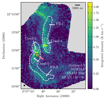
Figure 1: Velocity integrated HC3N $(10-9)$ emission. HC3N is integrated from 9.2 to 11.2 $\rm km\,s^{-1}$. White dashed contours correspond to the filaments identified in NH3 emission by P15 and S21. White solid contours outline the edges of the condensations labeled as in P15. The gray star marks the position of the protostar B5-IRS1. The black square represents the area observed with ALMA. The blue and red arrows indicate the direction of the blueshifted and redshifted lobes of the outflow in B5-IRS1 (Zapata et al., 2014).

Figure 2: Channel maps between 9.081 and 11.347 $\rm km\,s^{-1}$ for the NOEMA and 30m HC3N (10 – 9) spectral cube, in 0.206 $\rm km\,s^{-1}$ steps. The white dashed contours outline the NH3 filaments defined in P15. The white star represents the location of the protostar, which has a systemic velocity $\rm\textit{v}_{LSR}=10.2$ $\rm km\,s^{-1}$ (P15). The white ellipse at the bottom left corner represents the size of the beam. The white line in the top left channel map is a scalebar representing a length of 5000 au.

Figure 1 shows the integrated intensity of HC3N ($10-9$) emission. We overplot the contours from the NH3 condensations and filaments from P15 and S21, data which we further describe in Appendix A. HC3N ($8-7$) emission shows the same morphology, so this description applies to the ($8-7$) transition as well. The HC3N ($8-7$) integrated intensity map is shown in Appendix E.1. In general, HC3N ($10-9$) follows the shape of the NH3 (1,1) filaments, but its emission is more extended than the filaments, with a width of $\sim 40\arcsec$. Toward the northeast, the HC3N ($10-9$) emission continues beyond the edge of Fil-1 with a bright peak ($S/N>10$) near the edge of the NOEMA map, possibly connecting to the region defined as Clump 1 in S21. We note that, with the exception of the extended emission toward the north, HC3N emission is not detected in the extended coherent core defined in Pineda et al. (2010). The peak of HC3N ($10-9$) emission is located toward B5-IRS1, with two dimmer peaks in integrated emission, one centered on Cond-1 and the other at the southern edge of Cond-2.

Figure 2 shows the HC3N ($10-9$) channel maps in approximately 0.2 $\rm km\,s^{-1}$ steps. These channel maps show that HC3N ($10-9$) emission consists of two lanes of extended emission, one lane for each filament seen in NH3 (1,1), and peaks of emission located at the condensations, the protostar and toward the north of Fil-1 in the direction of Clump-1. Emission along the filaments is usually detected within 3 to 4 channels, except at locations such as Cond-1 and the protostar, where emission is present in more than 5 channels.

3.2 Morphology of H2CO line emission

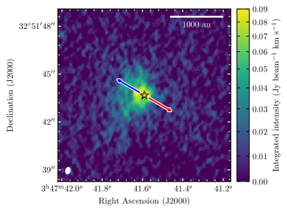
Figure 3: Velocity integrated image of H2CO from 8 to 12 $\rm km\,s^{-1}$. The black star represents the position of the protostar. The blue and red arrows indicate the directions of the blue and redshifted outflow lobes from Zapata et al. (2014). The scalebar indicates a length of 1000 au. The white ellipse in the bottom left corner represents the beam size. The primary beam of the image is out of the map.

Figure 4: Channel maps between 8.45 and 12.2 $\rm km\,s^{-1}$ for the ALMA H2CO (3_0,3 – 2_0,2) spectral cube, in steps of 0.25 $\rm km\,s^{-1}$. The white star represents the location of the protostar, which has a systemic velocity $\rm\textit{v}_{LSR}=10.2$ $\rm km\,s^{-1}$ (P15). The white dotted circle marks the extent of the primary beam. The white ellipse at the bottom left corners represents the beam size. The scalebar in the bottom left panel shows a 500 au length in the map.

Figure 3 shows the H2CO integrated image from 8 to 12 $\rm km\,s^{-1}$, and Fig. 4 shows channel maps of H2CO emission in approximately 0.2 $\rm km\,s^{-1}$ steps. The details of the observed C^18O emission morphology are described in Appendix C. The integrated image peaks toward the position of B5-IRS1 and shows stronger emission toward the east of the protostar than to the west, immediately hinting at asymmetries in the envelope. In the channel maps it is shown that the asymmetry is due to strong emission surrounding the protostar (within a $\sim 500$ au diameter) only toward the northeast, showing a curved shaped emission between 9.20 and 9.54 $\rm km\,s^{-1}$, which then decreases in intensity but expands toward the east in consecutive channels as it reaches the central velocity of the protostar $\rm\textit{v}_{LSR}=10.2$ $\rm km\,s^{-1}$ (P15). Channels from 9.7 to 10.3 $\rm km\,s^{-1}$ are affected by negative emission bowls adjacent to the extended emission, due to missing short-spacing data in the uv-plane. In the rest of the channels emission is more compact, and it is well recovered with the ALMA only observations. In higher velocity channels, from 10.45 to 10.95 $\rm km\,s^{-1}$ in fig. 4, there is asymmetric envelope emission toward the west of the protostar that is not evident in the integrated image. These features are evident in the image moments 1 and 2, which are shown in Appendix B. The peak of velocity dispersion is offset from the protostar to the east, where two sections with different velocities are joined. Also, there is an increase in velocity dispersion toward the southeast of the protostar, where emission is primarilly blueshifted. The moment maps and channel maps reveal that H2CO emission shows complex structure both spatially and spectrally.

3.3 HC3N (10 – 9) line fitting

We fit one Gaussian profile to the HC3N ($10-9$) line emission using the Python package pyspeckit (Ginsburg & Mirocha, 2011; Ginsburg et al., 2022). We describe our procedure in detail in Appendix D. In summary, we fit one Gaussian to all spectra with $S/N>5$ using moment maps to estimate the initial parameters, and then attempt the fit again using the results as initial guesses. The best fit parameters of each spectrum are shown in Fig. 5. We select four locations within each filament, labeled N-1 to N-4 and S-1 to S-4 for Fil-1 and Fil-2, respectively, to show their spectra in Fig. 6. The spectra are taken from a single pixel, which has a size of (0.6″)². Almost all spectra with $S/N>5$ are well fit using only one Gaussian, as seen in Fig. 6, with the exception of spectra located within a beam of the protostar’s position, which we explore further.

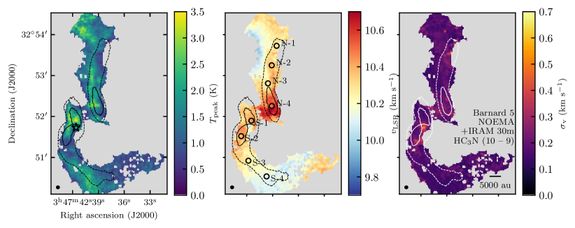
Figure 5: Peak intensity, central velocity, and velocity dispersion resulting from the Gaussian fit to the HC3N ($10-9$) spectra. Black and white dashed contours represent the edges of the filaments as defined in P15 and S21. The black and white solid contours mark the condensations as defined in P15. The black star marks the position of B5-IRS1. Black labeled circles indicate the position of the sampled spectra in Fig. 6. The black ellipse represents the beam size.

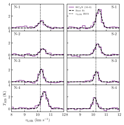
Figure 6: HC3N ($10-9$) spectra at selected locations within both filaments, ordered in position from north to south. Fil-1 spectra, labeled N-X, are on the left column and Fil-2 spectra, labeled S-X, are on the right. Purple lines show the spectra, whereas black curves show the best fit Gaussian curve for each.

At the position of B5-IRS1, there are several spectra within a radius of $\sim 4\arcsec$ where it is possible to fit a second component to the HC3N ($10-9$) emission that has a lower velocity than its surroundings. We describe this second fit in more detail in Appendix D.1. Previous works have been able to detect two and even three Gaussian components in NH3 emission (Choudhury et al. submitted, Chen et al., 2022), so it is expected that HC3N ($10-9$) can trace more than one component as well. We describe how we evaluated this second fit in Appendix D. According to our criteria, there are not enough spectra with a good enough two Gaussian fit to justify keeping it in our analysis. To separate the gas emission into more components in this region, we require observations with higher spectral resolution, as the Gaussians are covered by 3 or 4 channels only in most cases (Fig. 6), which is not enough to fit two Gaussians with certainty. Therefore, we stay with the one Gaussian fit for all regions for further analysis.

The central velocities $\rm\textit{v}_{LSR}$ of each spectrum, shown in Fig. 5 center, range from 9.8 to 10.7 $\rm km\,s^{-1}$. The uncertainties in $\rm\textit{v}_{LSR}$ are 0.025 $\rm km\,s^{-1}$ on average, ranging from 0.01 $\rm km\,s^{-1}$ at the center of the filaments and condensations, and increasing to approximately 0.05 $\rm km\,s^{-1}$ toward the edges of the filaments, where the $S/N\approx 5$. The $\rm\textit{v}_{LSR}$ map shows filament-scale gradients both parallel to the direction of the filaments and perpendicular to them. The central velocity within Fil-1 shows a velocity gradient parallel to the filament length of approximately 0.4 $\rm km\,s^{-1}$, starting from 10.3 $\rm km\,s^{-1}$ at the northern tip of Fil-1 and ending toward Cond-1 with 10.7 $\rm km\,s^{-1}$. Perpendicular to this filament, there is a gradient from lower to higher $\rm\textit{v}_{LSR}$ from east to west, starting from 10.0 $\rm km\,s^{-1}$ outside of the filament defined in NH3 and reaching 10.4 $\rm km\,s^{-1}$ on the opposite side. The gas within Fil-2 contour also shows a parallel velocity gradient, from 10.1 $\rm km\,s^{-1}$ in the south tip to 10.4 $\rm km\,s^{-1}$ in the north, reaching its maximum velocity within Cond-2 and 3. There is also a perpendicular gradient that is not apparent at first sight because it is smaller than the one present in its northern counterpart. The largest observed difference between the edges of Fil-2 is at the southern edge of Cond-3, where the $\rm\textit{v}_{LSR}$ goes from 10.4 $\rm km\,s^{-1}$ in the east to 10.2 $\rm km\,s^{-1}$ in the west. The HC3N ($10-9$) velocity gradients are produced by two continuous bodies of extended emission, one spatially correlated to Fil-1 and another to Fil-2, as seen in the channel maps (Fig. 2), and not from two or more spatially separated components in each filament.

Within a beam of the protostar there is a decrease in velocities with respect to its surroundings. At Cond-2 and 3, the velocity is around 10.4 $\rm km\,s^{-1}$, whereas around B5-IRS1, the velocity drops down to 10.0 $\rm km\,s^{-1}$. This sudden blueshift is partially due to the second component suggested at that location. However, the main peak at the location of the protostar is still blueshifted with respect to B5-IRS1 $\rm\textit{v}_{LSR}$ (Fig. 19).

The HC3N ($10-9$) velocity dispersion stays rather constant along both filaments, varying within beam areas randomly between 0.12 and 0.2 $\rm km\,s^{-1}$, except at the position of the protostar, where it increases suddenly to 0.5 $\rm km\,s^{-1}$, and toward the south of Cond-3, where the dispersion increases to $\sim 0.33$ $\rm km\,s^{-1}$. This is the reason why the peak of integrated emission (Fig. 1) is at the protostar’s location but the peak in the $T_{\mathrm{peak}}$ map (Fig. 5 left) is located inside of Cond-2. The protostar might produce the higher velocity dispersion around it, including toward Cond-3. Assuming the gas temperature in this region is 9.7 K (obtained from Pineda et al., 2021), the sound speed is $c_{\mathrm{s}}=0.18$ $\rm km\,s^{-1}$, so for the most part, the obtained velocity dispersion indicates the gas speed is mostly subsonic.

3.4 H2CO multicomponent line fitting

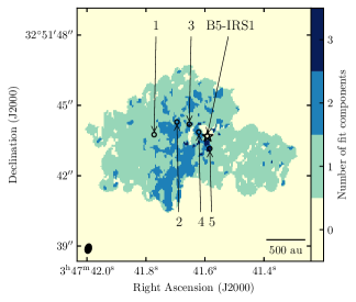
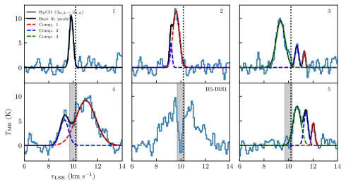
Figure 7: Results of the Gaussian fit to the ALMA H2CO spectra. Left: Number of components that best fit each H2CO spectrum according to the criteria described in Appendix D. The black ellipse in the bottom left corner represents the beam size. The black star marks the position of the protostar. Locations of sampled spectra are marked with empty black circles and labeled. Right: Selected H2CO spectra with the best fit Gaussian components. The spectra are taken from one single pixel. The data are plotted with a solid blue line. The dashed lines represent the best fit Gaussians, with red for the first component, blue for the second and green for the third. The black solid line represents the sum of all components. The gray vertical area marks the channels that were masked for the fit for spectra located within 0$\aas@@fstack{\prime\prime}$8  from the protostar. The dotted black vertical line marks the protostar’s $\rm\textit{v}_{LSR}$.

Figure 7 shows a sample of spectra from the ALMA H2CO emission cube, with increasing numbers representing decreasing distance to the protostar. The spectra are taken from a single pixel, which has an area of (0.003″)². The spectra show that close to and at the location of B5-IRS1, H2CO emission has more than one velocity component along the line-of-sight. This component multiplicity explains the sudden increase of velocity dispersion shown in the moment 2 map (Fig. 16 right).

We fit one, two, and three Gaussians to the H2CO line emission for each spectrum inside a mask created using all pixels with $S/N>5$. The details of the procedure, including the mask creation and the criteria to determine the number of components along each line of sight, are detailed in Appendix D. The general procedure is similar to the Gaussian fit in Sect. 3.3, but takes into account the possible effects of missing short- and zero-spacings in our interferometric data by masking the spectra between 9.7 and 10.3 $\rm km\,s^{-1}$ for pixels within a radius of 0$\aas@@fstack{\prime\prime}$8  from the protostar. An observation of these central spectra determines that these are the most affected by missing short-spacing data.

The number of Gaussian components that best fit the spectra are shown in Fig. 7 left and we show spectra with their corresponding best fits in Fig. 7 right. Most of the spectra are best fit using only one Gaussian, but closer to the protostar and toward the south, there are spectra that are better fit with 2 and 3 Gaussians. There are very few spectra that are best fit with 3 Gaussians, and most of these are located in the region where we mask the central velocity channels (between 9.7 and 10.3 $\rm km\,s^{-1}$) for the fit. Our criteria determined that in 0.1% of the spectra, located at a distance $<500$ au from the protostar, the best model has a probability lower than 95% of representing a considerable improvement in comparison to the other models. In paritcular, at the position of the protostar, the spectrum shows two peaks with a dip at the $\rm\textit{v}_{LSR}$ of the protostar. This dip is most probably caused by the missing short-spacing information, as it is located right on the channels that are masked. At this location, the Gaussian fits showed very large uncertainties for its parameters (more than 50%), and therefore the spectra within one beam of the protostar are left unfit.

4 Analysis

4.1 Gas flow from Barnard 5 dense core to the filaments

4.1.1 Comparison between core HC3N and NH3 velocities

We compared the HC3N ($10-9$) central velocities $\rm\textit{v}_{LSR}$ with the NH3 (1,1) $\rm\textit{v}_{LSR}$ found in P15 (shown in Fig. 15) to observe the relative motions of the chemically fresh gas with respect to the filaments. According to chemical models of cold, dark molecular clouds, NH3 and other nitrogen-bearing molecules are regarded as a “late-type” molecule, tracing advanced stages of gravitational core collapse, whereas HC3N and the cyanopolyyne (HC_2n+1N) molecule family trace chemically fresh gas (i.e., unprocessed by core collapse processes, Herbst & Leung, 1989; Bergin & Tafalla, 2007; Aikawa et al., 2001). We subtracted the NH3 $\rm\textit{v}_{LSR}$ from the HC3N ($10-9$) $\rm\textit{v}_{LSR}$, obtaining $\delta$$\rm\textit{v}_{LSR}$ $=v_{\mathrm{LSR,HC}_{3}\mathrm{N}}-v_{\mathrm{LSR,NH}_{3}}$. For this, we first convolved the HC3N ($10-9$) $\rm\textit{v}_{LSR}$ (Fig. 5 Center) to the spatial resolution of the NH3 (1,1) data (Table 1), using the photutils routine create_matching_kernel to obtain the matching kernel between the image beams and the astropy.convolution function convolve to smooth the map. Afterwards, we reprojected the spatial grid of the NH3 (1,1) central velocities image to the HC3N ($10-9$) spatial grid, using the reproject_exact routine from the reproject python package. We regridded the NH3 map to the HC3N ($10-9$) map grid because the pixel size of the NH3 map is about 1.5 times smaller than the HC3N ($10-9$) image pixel size. Finally, we subtracted the $\rm\textit{v}_{LSR}$ of NH3 from the HC3N ($10-9$) $\rm\textit{v}_{LSR}$.

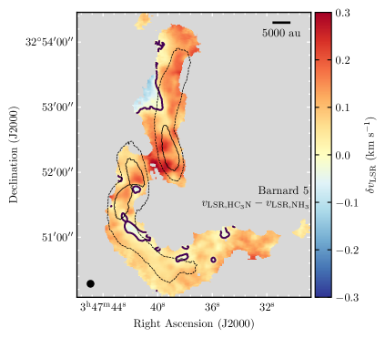
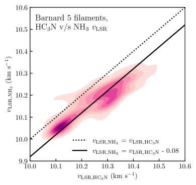
Figure 8: Difference between HC3N ($10-9$) line emission and NH3 (1,1) line emission central velocities in both filaments of Barnard 5. Left: Spatial map showing the difference of HC3N ($10-9$) central velocities with respect to NH3 (1,1) velocities. Black thick contours mark the positions where the difference is 0. The resolution of the HC3N ($10-9$) data is on the lower left corner. The dotted contours show the filaments and the black solid contours outline the condensations as defined in P15 and S21. Right: v${}_{\mathrm{LSR},\mathrm{HC}_{3}\mathrm{N}}$ versus v${}_{\mathrm{LSR},\mathrm{NH}_{3}}$ Distribution of the velocity difference shown using its KDE. The dashed vertical line represents the 1:1 line, and the solid line is shifted by -0.08, which is the median value of the difference between both velocities.

Figure 8 left shows the resulting $\delta$$\rm\textit{v}_{LSR}$ in the image plane. The map shows that HC3N ($10-9$) is consistently redshifted with respect to NH3 except for a few locations, mostly without systematic variations within the NH3 filament regions. The median value of $\delta$$\rm\textit{v}_{LSR}$ is $0.08^{+0.06}_{-0.05}$ $\rm km\,s^{-1}$. This difference is more than 3 times larger than the average uncertainty for $\delta$$\rm\textit{v}_{LSR}$, which is dominated by the uncertainty of the HC3N ($10-9$) $\rm\textit{v}_{LSR}$ (Sect. 3.3). Toward the southern tip of Cond-1, HC3N ($10-9$) $\rm\textit{v}_{LSR}$ is larger than NH3 (1,1) $\rm\textit{v}_{LSR}$ by $\approx 0.28$ $\rm km\,s^{-1}$, but the rest of the spectra are consistent with the median value. Figure 8 Right shows the HC3N ($10-9$) central velocities versus the respective NH3 $\rm\textit{v}_{LSR}$ at the same location, estimated using a two-dimensional Gaussian Kernel Density Estimate (KDE) obtained with the scipy.stats python package gaussian_kde function (Virtanen et al., 2020) assuming all pixels have the same weight. The KDE shows there is an approximately linear relation between both $\rm\textit{v}_{LSR}$ with a shift of $-0.08$ $\rm km\,s^{-1}$. This comparison shows that HC3N ($10-9$) follows a different kinematic component of the gas in Barnard 5 than NH3.

There are a few locations where HC3N ($10-9$) emission is blueshifted with respect to NH3 (1,1) emission. At the right of Fil-1, $\delta$$\rm\textit{v}_{LSR}$ drops down to $\approx-0.1$ $\rm km\,s^{-1}$. Also, just below Cond-3 in Fil-2, there is a region where $\delta$$\rm\textit{v}_{LSR}$ also reaches $\approx-0.1$. The blueshifted emission at these positions, which are elongated along the filaments, suggest there is a perpendicular velocity gradient of HC3N with respect to NH3. In particular, there is a sudden shift from positive to negative $\delta$$\rm\textit{v}_{LSR}$ at the location of the protostar, reaching down to $\delta$$\rm\textit{v}_{LSR}$ $\approx-0.06\rm km\,s^{-1}$. The area of the reversal is approximately the NH3 (1,1) beam size. Comparing the HC3N ($10-9$) fit with the NH3 (1,1) fit (Fig. 15) shows that both molecules present a sudden decrease in $\rm\textit{v}_{LSR}$ at that location, but the difference between $\rm\textit{v}_{LSR}$ in this position and its surroundings is larger for HC3N ($10-9$) than for NH3.

4.1.2 HC3N velocity gradients

In Fig. 5 center, there is a velocity gradient perpendicular to Fil-1 observed in HC3N ($10-9$) central velocities. The perpendicular gradient in Fil-2 is overshadowed by a strong gradient running parallel to the filament length. We calculated the velocity gradients $\nabla$$\rm\textit{v}_{LSR}$ present in the map to determine the direction of gas flow at the positions where the condensations and the protostar are and to determine if there are gradients perpendicular to Fil-2 that are hidden by an analysis by eye. We employed the same procedure used to calculate velocity gradients in Barnard 5 NH3 (1,1) emission by Chen et al. (2022), which is described in detail in Chen et al. (2020b). In summary, we calculated the gradient pixel-by-pixel by fitting a plane centered around the pixel, using a square aperture with a width of 2 beams ($\approx 8\arcsec$ width), to ensure the capture of velocity gradients across non-correlated regions. We only fit pixels which have a number of neighboring pixels equivalent to one third of the aperture area available to ensure the quality of the fit.

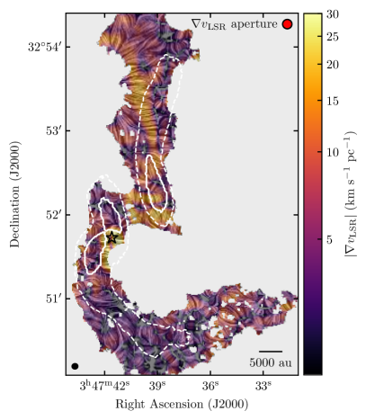
Figure 9: Velocity gradient intensities $|\nabla\rm\textit{v}_{LSR}|$ calculated from the Gaussian fit to HC3N ($10-9$) emission, with the gradient directions visualized as an overplotted texture using line integral convolution (LIC, Cabral & Leedom, 1993). The black star indicates the position of B5-IRS1. The black ellipse in the bottom left corner represents the beam size. The red circle at the top right corner represents the area used to calculate the gradients. White dashed contours outline the NH3 filaments (; ). White solid contours outline the edges of the condensations (P15). The scalebar at the bottom right corner represents a physical distance of 5000 au.

Figure 9 shows the resulting HC3N ($10-9$) $\nabla$$\rm\textit{v}_{LSR}$ visualized using line integral convolution (LIC, Cabral & Leedom, 1993) textures over the absolute magnitude of the gradient $|\nabla\rm\textit{v}_{LSR}|$. We used the LicPy package (Rufat, 2017) to generate a texture that represents the directions of the gradients, and then overlaid the resulting texture. The uncertainty in $|\nabla\rm\textit{v}_{LSR}|$ is between 0.3 and 1 $\rm km\,s^{-1}$ pc^-1 and increases toward the edges of the HC3N ($10-9$) emitting region. We focus our discussion on a qualitative description of the resulting $\nabla$$\rm\textit{v}_{LSR}$ map.

The vector field is well ordered within the brightest HC3N emissions, in particular, in and around the condensations and filaments defined by NH3 contours and toward the bright emission toward the north of the map (which connects with Clump-1 from S21, ). Figure 9 reveals that gas in and around both filaments have both parallel and perpendicular gradients.

The $\nabla$$\rm\textit{v}_{LSR}$ field reveals the flow of gas toward the condensations. Within the contours of Fil-1, the perpendicular gradients are toward the edges of HC3N emission with $|\nabla\rm\textit{v}_{LSR}|\,\approx 12-15$ $\rm km\,s^{-1}$ pc^-1). The vector field reveals a strong (—$\nabla$$\rm\textit{v}_{LSR}$ $|\,\approx 20$ $\rm km\,s^{-1}$ pc^-1 ) parallel gradient of $\sim 8000$ au in length above Cond-1. The vector field is particularly well ordered at the north of Fil-1, where there is HC3N emission which could possibly connect to Clump-1 toward the north. Cond-1 is surrounded by flows with magnitudes between 25 and 30 $\rm km\,s^{-1}$ pc^-1. that point toward its center, but at the center of the condensation the flow stagnates (i.e., drops to 0 $\rm km\,s^{-1}$ pc^-1). This indicates HC3N moves inward to Cond-1 from all directions.

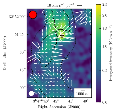
Figure 10: Zoom of the integrated intensity map toward Cond-2, -3 and the protostar, with the $\nabla$$\rm\textit{v}_{LSR}$ vector orientations from Fig. 9 shown with white lines. The black line at the top represents a gradient magnitude of 10 $\rm km\,s^{-1}$ pc^-1. The black star indicates the position of B5-IRS1. The white ellipse in the bottom left corner represents the beam size. Black dashed contours outline the NH3 filaments (; ). Black solid contours outline the edges of the condensations (P15). The red circle at the top left corner represents the area used to calculate the gradients. The scale bar at the bottom right marks a length of 1000 au.

The $\nabla$$\rm\textit{v}_{LSR}$ calculation also reveals the parallel flow of gas in Fil-2 that was not evident by eye. Toward the south of Cond-3, most of Fil-2 shows perpendicular gradients with $|\nabla v_{\mathrm{LSR}}|$ between 3 and 10 $\rm km\,s^{-1}$ pc^-1, much lower than the perpendicular gradients at Fil-1. The western edge of Cond-3 presents the strongest velocity gradient of the map ($\nabla v_{\mathrm{LSR}}\approx 40$ $\rm km\,s^{-1}$ pc^-1) and its direction is parallel to the filament. Both condensations (Cond-2 and -3) show stagnating flows within them. This indicates that gas flows from the outside in, as in the case of Cond-1. Most notably, a zoom into the condensations within Fil-2, shown in Fig. 10, reveals that the gradient direction curves toward the protostar and the parallel gradient ends there as well. This plot suggests that fresh gas, traced by HC3N, flows toward the protostar, and the large-scale flow along the filament is hence shared by the protostar, Cond-2 and Cond-3.

4.1.3 Mass inflow from Barnard 5 dense core to the filaments

We estimated the mass transport and the infall rate from the flows traced by HC3N emission. In Choudhury et al. (submitted), they estimate an infall rate $\dot{m}$ for Fil-1 of $1.1\times 10^{-4}$ $\rm M_{\sun}$ yr^-1 and for Fil-2 of $1.8\times 10^{-4}$ $\rm M_{\sun}$ yr^-1. We used the same geometry for both filaments and their Eq. 8 to estimate $\dot{m}$:

$$\dot{m}=S\rho v_{\mathrm{inf}},$$ (1)

where $S$ is the surface area where infall occurs, $\rho$ is the total mass volume density within the surface area and $v_{\mathrm{inf}}$ is the estimated infall velocity.

We obtained $\rho=n(\mathrm{H}_{2})\mu m_{\mathrm{H}}$ by using the line ratio between HC3N ($10-9$) and ($8-7$) molecular transitions. This procedure is described in detail in Appendix E. In summary, we obtained a number density $n(\mathrm{H}_{2})\approx 10^{5}$ cm^-3 based on the non-LTE radiative transfer code RADEX (van der Tak et al., 2007). The mean difference in velocity, which is defined as half the difference in $\rm\textit{v}_{LSR}$ across a filament, is $v_{\mathrm{inf}}=0.2$ $\rm km\,s^{-1}$ for Fil-1 (the same as the one observed in Choudhury et al. submitted) and 0.1 $\rm km\,s^{-1}$ for Fil-2 (Sect. 3.3). The resulting mass infall rate is $\dot{m}=4.3\times 10^{-5}$ $\rm M_{\sun}$ yr^-1 in Fil-1 and $\dot{m}=3.5\times 10^{-5}$ $\rm M_{\sun}$ yr^-1 for Fil-2, about 3 times lower than the Fil-1 infall rate found in Choudhury et al. (submitted). The difference is due to the obtained $n(\mathrm{H}_{2})$ in both works. We estimated $n(\mathrm{H}_{2})$ using our observed HC3N transitions (Appendix E). On the other hand, Choudhury et al. (submitted) used the filament masses from S21, which in turn were calculated by comparing Barnard 5’s NH3 emission and the JCMT 0.45 mm emission.

4.2 Infall from envelope to disk scales

4.2.1 Clustering of physically related structures in H2CO

We separated the different Gaussian components found in H2CO in Sect. 3.4 into clusters, which helps to interpret the kinematic properties of the B5-IRS1 envelope. It is challenging to do this separation by eye, especially where there are two components in the same line of sight that can belong to two different components indistinguishably. For example, in the boundary between blueshifted and redshifted sides of the H2CO emission, toward the south and east of the protostar, there are two Gaussian components with velocities blueshifted with respect to the protostar’s $\rm\textit{v}_{LSR}$ (see Fig. 7 Left). Also, the locations where there are three Gaussian components are small and sparse, as well as spectra at the east and west edges of the H2CO emission. It is possible that the additional fitted components are either noise or extended emission that is not fully sampled due to missing short- and zero-spacing observations. We describe our procedure in Appendix F, where we also show the resulting clusters in Fig. 23. In summary, we employed the density-based spatial clustering of applications with noise (DBSCAN) algorithm to separate the different physical components in position-position-velocity space.

The two largest clusters returned by DBSCAN (Groups 0 and 1 from Fig. 23) contain about 90% of the points not categorized as noise. The largest cluster is a group of points that are all blueshifted with respect to the protostar’s $\rm\textit{v}_{LSR}$ (10.2 $\rm km\,s^{-1}$), and the second largest, a fully redshifted group. We refer to these two groups as blueshifted and redshifted clusters throughout the rest of this work. More details about these two clusters are in Appendix F. The central velocities of the Gaussian fits belonging to each of these clusters are shown in Fig. 11. The blueshifted cluster has a velocity gradient toward lower (more blueshifted) velocities as it gets closer to the protostar. This gradient is stronger for higher declinations. The redshifted cluster has an increase in velocity when it gets closer to the protostar.

The remaining three clusters represent $\approx 10$% of the points not considered noise. The clustering algorithm is able to assign one of the two blueshifted Gaussian components toward the south of the protostar (Fig. 7) to the blueshifted cluster and leave the other as another group (Group 3 from Fig. 23). This allows us to observe the velocity gradient more clearly. The main difference between the largest clusters and groups 4 and 5 is these two last groups show highly blueshifted and redshifted $\rm\textit{v}_{LSR}$ very close to the protostar, representing a jump in the velocity gradient of groups 0 and 1. Group 3 has a central velocity of 10.8 $\rm km\,s^{-1}$ and group 4, of 9.2 $\rm km\,s^{-1}$. Groups 3, 4, and 5, as well as possibly part of the points categorized as noise, could be emission coming from other mechanisms observed in H2CO, such as inner gas disk rotation or a more extended envelope, that due to the resolution or the missing short-spacing data cannot be fully observed. Group 3, for example, shows a central velocity redshifted with respect to the protostar at the same position as the redshifted high-velocity C^18O emission, described in Appendix D. We suggest the high-velocity C^18O and H2CO emission components trace the protostellar disk kinematics. Another possibility is that within 500 au from the protostar H2CO gas is optically thick, which would cause self-absorbed emission that is being fitted as separate velocity components and then categorized as the purple and orange groups (labeled as 3 and 4, respectively) by the algorithm.

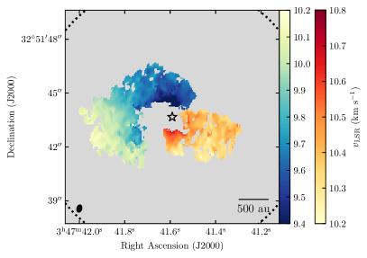
Figure 11: Central velocities for the blueshifted and redshifted clusters found using the methods described in Appendix F. The colorbar from yellow to blue corresponds to the velocities for blueshifted cluster, whereas from yellow to red corresponds to the redshifted cluster. The black ellipse in the bottom left corner represents the beam size. The black star represents the position of the protostar. The black dashed circle (only seen at the corners) represents the size of the primary beam. We note that the velocity ranges for both envelope components are not symmetric.

4.2.2 Streamline model of the H2CO clusters

The two main clusters found by DBSCAN each have a gradient where velocity (with respect to the protostar) increases as distance decreases, similar to streamers confirmed kinematically toward other protostars, for example Per-emb-2 (Pineda et al., 2020) and Per-emb-50 (Valdivia-Mena et al., 2022). We determined if the kinematics of the blueshifted and redshifted components are consistent with streamers infalling toward the protostellar disk of B5-IRS1.

First, we checked if H2CO emission is tracing or is affected by the outflow. In some protostellar sources, H2CO traces the outflow or the extremely high-velocity jet (Tychoniec et al., 2021). The position of the blueshifted component is at the east of the protostar, in the same side as the blueshifted outflow cone, and the redshifted component and outflow cone are both toward the west (Fig. 3). However, the velocity gradients of the blueshifted and redshifted components are opposite to the gradient expected for an outflow. For the blueshifted component, $\rm\textit{v}_{LSR}$ goes from 10.1 $\rm km\,s^{-1}$ at a distance of about 1000 au to 9.2 $\rm km\,s^{-1}$ at approximately 200 au from the protostar. This means that it is accelerating toward more blueshifted velocities with respect to the protostar’s $\rm\textit{v}_{LSR}$ (10.2 $\rm km\,s^{-1}$) as distance decreases. For the redshifted component, $\rm\textit{v}_{LSR}$ is approximately 10.3 $\rm km\,s^{-1}$ at about 1000 au and accelerates to 10.6 $\rm km\,s^{-1}$ at a distance of 300 au, which also represents an acceleration with respect to the protostar’ $\rm\textit{v}_{LSR}$ with decreasing distance. For an outflow, the velocity with respect to the protostar increases with distance, opposite to the behavior of $\rm\textit{v}_{LSR}$ shown by both components. Therefore, the motion observed in these H2CO components is not consistent with outflow motion.

Second, we checked the velocity dispersion $\sigma_{\mathrm{v,fit}}$ of the Gaussians in the blueshifted and redshifted clusters and compare them to the thermal sound speed. Nonthermal velocity dispersion larger than the sound speed can indicate that the motion traced by H2CO is not simple envelope infall, but can be affected by turbulence and shocks produced by the outflow in the same line of sight. We describe the procedure and the resulting nonthermal velocity dispersion of the blueshifted and redshifted clusters in Appendix F.1. The velocity dispersion is subsonic for the majority of the emission in both components, but it becomes trans-sonic for emission within $r<600$ au from the protostar. This suggests that within this radius, H2CO gas is possibly affected by the outflow. Additionally, there is a larger density of trans-sonic emission for the redshifted component. This is due to the smaller area covered by this component and the fact that it is mostly contained in the observed direction of the outflow cone. The H2CO gas contained in this cluster is therefore contaminated by outflow emission. For this reason, we leave the redshifted component as a streamer candidate and do not do further analysis on it in this work.

We modeled the kinematics of the blueshifted cluster observed with H₂CO emission to confirm that the velocity gradient observed in Fig. 11 is consistent with streamer motion, using the analytic solution for material falling from a rotating, finite-sized cloud toward a central object, dominated by the gravitational force of the latter. We used the analytic solutions of Mendoza et al. (2009), previously used by Pineda et al. (2020) and Yen et al. (2014). The model’s input and output are described in detail in Valdivia-Mena et al. (2022), here we describe briefly the input parameters used for this source.

The streamline model requires the central mass that is causing the gravitational pull as input, which is the sum of the masses of the protostar, disk, and envelope, $M_{\mathrm{tot}}=M_{*}+M_{\mathrm{disk}}+M_{\mathrm{env}}$. We estimate the protostellar mass by fitting a two-dimensional Gaussian to individual C^18O (2 – 1) channels and comparing the resulting distance and velocity (with respect to B5-IRS1) with the Keplerian curves predicted for different protostellar masses. We describe the process in detail in Appendix G. Through this analysis, we obtain a central protostellar mass $M_{*}\approx 0.2$ $\rm M_{\sun}$. For the disk mass, we use an upper limit of $M_{\mathrm{disk}}=0.03$ $\rm M_{\sun}$ found by Zapata et al. (2014). As this value is small, it does not have a significant effect on the resulting parameters of the model. We use an envelope mass of $M_{\mathrm{env}}=0.27$ $\rm M_{\sun}$ from Andersen et al. (2019), obtained through the comparison of continuum observations from the Submillimeter Array (SMA) and single-dish observations. The disk and envelope mass are corrected for a distance to B5 of 302 pc (Zucker et al., 2018), as the original masses reported in those works are calculated with a distance of 240 pc.

To decrease the number of free parameters to explore, we fixed the inclination angle $i$ and position angle $PA$ of the rotating cloud using previous information from the outflow and disk in B5-IRS1. The outflow inclination angle is -13°(where 0°is on the plane of the sky and positive is away from the observer, Yu et al., 1999) and its position angle is 67$\aas@@fstack{\circ}$1 (where 0°is north, Zapata et al., 2014). Assuming the disk belongs in a plane perpendicular to the outflow, then $PA=157\aas@@fstack{\circ}1$ (from north, if 0°is a disk aligned in the north to south direction) and $i=13\degr$ (from the plane of the sky). In this setup, the angular velocity vector of the disk $\@vec{\omega}$, and therefore of the streamer, points toward the southwest, away from the observer.

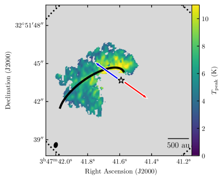
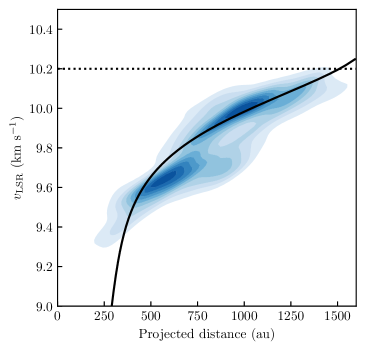
Figure 12: Streamline model that best fits the observed blueshifted envelope component in H₂CO line emission. In both image and velocity space, the black curve represents the streamline model solution that best describes the bulk motion of the streamer. Left: Peak main beam temperature $T_{\mathrm{peak}}$ for each pixel in the blue component found with DBSCAN. The blue and red arrows show the direction of the blue and red outflow lobes from Zapata et al. (2014), respectively. The black ellipse in the bottom left corner represents the beam size. The black star represents the position of the protostar. The black dashed circle represents the size of the primary beam. Right: central velocity KDE for the blueshifted envelope plotted against the projected distance from the protostar.

We explored the initial position ($r_{0}$, $\vartheta_{0}$ and $\varphi_{0}$) and velocity $\mathrm{v}_{r,0}$ to find the set that best fits the observed positions and velocities. We manually changed the parameters to obtain streamline model curves that resemble the shapes of both the peak emission and the line-of-sight velocities of each component (Fig. 12). As the infall motion covers a large area in the image plane and does not look like a thin, collimated streamer (as in the cases of Pineda et al., 2020; Valdivia-Mena et al., 2022), there must be a family of solutions that describe the whole streamer. We find the streamline model that best describes the bulk motion of the blue cluster, that is, the one that best fits the observed velocities and is contained within the emission region of the blue cluster in the image plane. Its parameters are in Table 2. We explored other combinations of $r_{0}$, $\vartheta_{0}$ and $\varphi_{0}$ to find other possible solutions. The parameters presented in Table 2 are the ones that replicate best the approximate shape of the streamer in the image plane and the velocities at the same time.

Figure 12 shows the projected trajectory of the streamline model over the blue cluster peak temperature (left panel) and over the KDE of the velocities and projected distance in the streamer (right panel). We used the KDE implementation in the python package SciPy (Virtanen et al., 2020) over the resulting central velocities obtained for the cluster. The streamline model reproduces the velocity gradient shown in the KDE. The resulting centrifugal radius $r_{\mathrm{c}}$ (as defined in Mendoza et al., 2009), which is the distance down to which the movement can be modeled with constant angular momentum, is 249 au. This radius is an upper limit to the location where the mass flow ends, as any process that can affect the streamer motion, such as interaction with the outflow (as mentioned in Appendix F.1), will decelerate the gas flow and therefore, reduce its angular momentum. This radius is consistent with the infall material being deposited at gas disk-scale distances from the protostar: the dust disk has an estimated radius $\sim 50$ au using mm-continuum emission (Yang et al., 2021), and although we cannot define a gas disk radius with our C^18O data (Appendix G), the gas disk extension tends to be much larger than what can be seen in dust emission, up to several 100 au (Miotello et al., 2022, and references within).

Table 2: Parameters of the streamline model that reproduce best the H₂CO blueshifted cluster and resulting centrifugal radius.

Parameter	Unit	Value
$\vartheta_{0}$	deg	101
$\varphi_{0}$	deg	65
$r_{0}$	au	2810
$v_{r,0}$	$\rm km\,s^{-1}$	0
$\Omega_{0}$	s-1	$2.8\times 10^{-13}$
$i$	deg	13
P.A.	deg	157.1
$r_{\mathrm{c}}$	au	245

5 Discussion

5.1 Chemically fresh gas feeds the filaments

In this work, we present new HC3N ($10-9$) and ($8-7$) emission data within the coherent core of B5. Our results and analysis of HC3N ($10-9$) velocities and its comparison to previous results with NH3 (1,1) emission indicate that HC3N traces chemically fresh gas infalling toward the filaments and condensations, following the curvature of the filaments. We explain our reasoning below.

Figure 8 shows that HC3N emission is consistently redshifted with respect to NH3. The systematic difference in centroid velocities shows these molecules do not trace the same material within B5. As mentioned in Sect. 4.1.1, HC3N traces material unprocessed by core collapse, whereas NH3 is expected to be more abundant in regions where core collapse is underway. Previous results in other star formation regions also show kinematic differences between carbon-chain molecules and nitrogen bearing molecules (e.g., Friesen et al., 2013). Therefore, HC3N traces the kinematics of chemically fresh material with respect to the main filamentary structure.

That being said, the velocities shown by HC3N emission are consistent with infall from the B5 dense core to the filaments and condensations. The Gaussian fit to the HC3N spectra (Fig. 5) and the further velocity gradient analysis (Sect. 4.1.2) reveal that both filaments show a velocity gradient running parallel to the filaments’ full length. The velocity gradients of the filaments run in opposite directions: in Fil-1, the global gradient runs from lower $\rm\textit{v}_{LSR}$ toward the north to higher $\rm\textit{v}_{LSR}$ in the south, with the highest $\rm\textit{v}_{LSR}$ in Cond-1, whereas in Fil-2 the global gradient starts from lower $\rm\textit{v}_{LSR}$ at the south and increases toward the north, following the curvature of the filament. We interpret this as a flow of gas running along the direction of the filaments toward the condensations. NH3 (1,1) emission also shows parallel velocity gradients with the same orientations (Fig. 15, S21, ). These large-scale parallel velocity gradients are similar in to those found in other filament, such as NGC 1333 (Hacar et al., 2017; Chen et al., 2020b) and L1517 (Hacar & Tafalla, 2011). Assuming filament lengths of 0.24 pc for Fil-1 and 0.31 for Fil-2 from S21, the average gradients along each filament are approximately 1.7 $\rm km\,s^{-1}$ pc^-1 and 1.0 $\rm km\,s^{-1}$ pc^-1, respectively. These values resemble the magnitude of the parallel velocity gradients found in other filaments and fibers ($\sim 1$ $\rm km\,s^{-1}$ pc^-1, e.g., Kirk et al., 2013; Fernández-López et al., 2014; Chen et al., 2020b).

The velocity gradients running perpendicular to the filament orientations are suggestive of infall from the B5 dense core to the filaments themselves. Fil-1 and the HC3N emission just outside of it to the north and to the east show an east-west velocity gradient that crosses the full width of the filament (Fig. 5 center) whereas small-scale perpendicular gradients in Fil-2 are revealed when calculating $\nabla$$\rm\textit{v}_{LSR}$ at scales of 2.5 times the beam (Fig. 9). This type of velocity gradient is consistent with the contraction of a sheet-like cloud, as argued in filament simulations (Chen et al., 2020a), as well as rotation around the filaments’s main axis. This type of gradient has been observed in other filaments, for example, within Perseus and Serpens molecular clouds (Fernández-López et al., 2014; Dhabal et al., 2018). We interpret the velocity gradient as infall dominated gas because these filaments are not supported against gravitational collapse given the turbulence in the B5 core, unless a magnetic field is present, and show signs of contraction (S21). Infall of material toward the center of the filaments has been suggested for B5 in previous works which analyze the kinematics of NH3 (1,1) (Schmiedeke et al., 2021; Chen et al., 2022, Choudhury et al. submitted). Our results support the interpretation that the additional components found by Choudhury et al. (submitted) are, as suggested, signs of infall from the coherent core. We suggest that HC3N is more sensitive to the flow of mass from the Barnard 5 core to the filaments, whereas NH3, as it is a later type molecule, only traces the flow of gas within the filaments toward the condensations and differentiates regions of subsonic and supersonic turbulent motions (Pineda et al., 2010).

5.2 A streamer toward B5-IRS1

The two main H2CO emission clusters in position-position-velocity space found in Sect. 4.2.1 have velocity gradients consistent with infall motion. We confirmed that most of the emission on these structures is not affected by the outflow, at least beyond $\sim 600$ au from the protostar. The nonthermal dispersion decreases as the distance to the protostar increases for both clusters (Fig. 24). Most of the spectra located at distances $>600$ au have subsonic $\sigma_{\mathrm{v,nt}}$. There are, however, some spectra with trans-sonic velocity dispersion ($\mathcal{M}_{s}\gtrsim 1$) within 600 au of the protostar. This result suggests that H2CO gas located closer to the protostar is becoming affected by the outflow, which increases $\sigma_{\mathrm{nt}}$.

We were able to confirm the infall nature of the blueshifted streamer using the streamline model. The best fit solution starts from the outer edge of the blue cluster’s emission with null initial radial velocity. We note that the blue streamer is not a thin, long structure such as other streamers in the literature, but more similar to a bulk of gas infalling due to gravity. Moreover, as the channels that trace the streamer at a distance of about 2800 au from the protostar are affected by missing short-spacing data (as seen in Fig. 4, between 9.6 and 10.4 $\rm km\,s^{-1}$), it is possible we miss some of the extent of this bulk. The spatial width of the emission we do trace suggests that the component could be fitted by a family of streamlines. We only took the one that best matches the general velocity KDE that passes through the emission seeen in the plane of the sky, because this allowed us to confirm its infalling nature. Nevertheless, this streamer has a similar length ($\approx 2800$ au) to other streamers found toward Class I protostars (Yen et al., 2014; Valdivia-Mena et al., 2022).

Understanding the kinematic nature of envelope emission helps disentangle the chemical history of the protostar. A previous work by van’t Hoff et al. (2022) shows H^13CO+ (2 – 1) emission with a ridge-like structure toward the east of B5-IRS1, similar to the arc shaped blueshifted envelope cluster. They suggest that emission is either associated with an extended water snowline due to a previous accretion burst in this source, or the larger protostellar envelope. We compare the H2CO blueshifted envelope component with the H^13CO+ emission from van’t Hoff et al. (2022) in Appendix H. Both emissions overlap in the image plane, although H^13CO+ is more extended than H2CO. The velocity gradients are the same and there are no significant differences between the central velocities of both molecular emissions. Therefore, we confirm that H^13CO+ traces the envelope’s infalling motion and not an extended snowline due to an accretion burst in this source. This suggest that using the H^13CO+ emission without further kinematic information about the source can overestimate the water snowline distance. This example highlights the importance of the kinematic information toward a source to interpret its chemical history.

Confirming the streamer nature of the redshifted cluster is not as clear as for the blueshifted cluster. The red cluster could be described using the same initial distance and angular velocity as the blue cluster streamline model. However, this model assumes that the blue and red clusters are part of the same envelope (i.e. have the same $\Omega_{0}$, $i$ and $PA$), which cannot be confirmed with the available data. Also, it is possible that the red streamer is more affected by missing short-spacings of our interferometric data than the blue streamer. In projected distance (i.e. in the RA-DEC plane), the streamline model of the blue streamer measures approximately 12″, so if the red streamer emission extends as suggested by the streamline model, the MRS of our data ($\approx 6\arcsec$, Sect. 2.4) does not allow us to detect its emission and we are only detecting the brightest part. Therefore, the classification of “streamer” is left as tentative for the red component of the envelope, and ALMA ACA observations of this region are required to confirm its streamer nature. If confirmed, B5-IRS1 would have twin streamers instead of only one as in other protostellar sources. This is similar to the case of L1489 IRS (Yen et al., 2014), a Class I source with two streamers observed in C^18O (2 – 1), and of [BHB2007] 11 (Alves et al., 2020), a Class I/II source with two streamers detected with ^12CO (2 – 1). Simulations show that when a protostar is still embedded in its natal core, there are several asymmetric channels from which matter is funneled (e.g., Padoan et al., 2014; Kuffmeier et al., 2017, 2023), but in most cases, only one streamer is observed (e.g., Pineda et al., 2020; Garufi et al., 2022; Valdivia-Mena et al., 2022). The fact that we do not see multiple streamers in other sources does not mean that they are not present, it is possible that their column density is too low to be detected. Further discoveries of streamers will help determine if dual streamers are a common occurrence or an exceptional phenomenon.

5.3 Connection between large scale and small scale infall

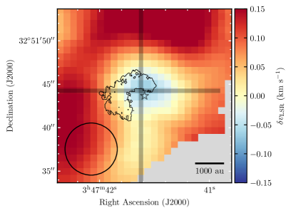
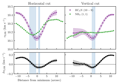
Figure 13: Left: Zoom into $\delta$$\rm\textit{v}_{LSR}$ from Fig. 8 toward the position of the protostar. The black contours mark the region of the blue streamer found in Sect. 4.2.1. The horizontal and vertical black lines show the positions of the horizontal and vertical cuts for the plots on the right. The black circle at the lower left corner represents the beam size of the NH3 (1,1) observations. Right: Horizontal and vertical cuts of HC3N $\rm\textit{v}_{LSR}$ and NH3 $\rm\textit{v}_{LSR}$. The purple points with the purple area represent the HC3N ($10-9$) $\rm\textit{v}_{LSR}$ and its associated uncertainty after smoothing to reach the same resolution as the NH3 (1,1) $\rm\textit{v}_{LSR}$. The green points represent the NH3 (1,1) $\rm\textit{v}_{LSR}$ (the uncertainties are roughly the size of the points). The black curves and black areas represent the difference between HC3N ($10-9$) NH3 (1,1) $\rm\textit{v}_{LSR}$. The blue areas represent the location covered by the blue streamer.

In this work, we observed infall motions both at large scales, from the core to the filaments, and at small scales, from the protostellar envelope to the disk. Even if the difference in resolution for these datasets is approximately tenfold, our results suggest that the confirmed streamer’s origin lies within the fresh gas flowing from the B5 dense core. We discuss the connection between these infall mechanisms.

Figure 8 shows that the relative velocity of HC3N with respect to NH3 reverses at the position of the protostar, showing a blueshifted zone about the size of the NH3 beam. Interestingly, zooming into this region (Fig. 13 Left) reveals that this blueshifted area is located approximately at the position of the blue streamer found using H2CO with ALMA data, which has a 10 times smaller beam. To prove that the difference between HC3N and NH3 bluehsifted emission is significant, we show horizontal and vertical cuts of HC3N ($10-9$) and NH3 (1,1) $\rm\textit{v}_{LSR}$, centered at the position of the minimum $\delta$$\rm\textit{v}_{LSR}$, in Fig. 13. The difference between both molecules’ velocities is larger than the uncertainties of each fit: HC3N decreases within a beam-sized area at the location of the protostar by approximately 0.4 $\rm km\,s^{-1}$ with respect to its surroundings, whereas NH3 has a decrease in $\rm\textit{v}_{LSR}$ of about 0.1 $\rm km\,s^{-1}$ in the same region, only evident in the horizontal cut. Therefore, HC3N ($10-9$) emission has larger variations around the protostar than NH3 (1,1). Moreover, this region coincides with where the AIC suggests two Gaussians fit HC3N better than one Gaussian, but with not enough certainty (Fig. 20). The low certainty from the AIC criterion is caused by insufficient spectral resolution to separate both components, but it suggests that, with better spectral resolution, we might be able to disentangle two velocity components, one related to the kinematics of the core gas infalling toward the filaments, and another, more blueshifted gas component which could trace the streamer. Overlaying the region where the streamer is present (blue vertical bands in Fig. 13 Right), the streamer is close to the location of the minimum $\rm\textit{v}_{LSR}$ for HC3N. This coincidence suggests that HC3N is sensitive to the infall motions close to the protostar in the dense core.

The velocity gradients seen in HC3N also suggest the streamer is connected to chemically fresh gas. The strongest HC3N velocity gradients are present toward Cond-1 and the protostar. A zoom into the north of Fil-2, shown in Fig. 10, shows that gas flows along the filaments and reaches the condensations and the protostar, where they distribute between the three, as seen from the change in direction in the $\nabla$$\rm\textit{v}_{LSR}$ vectors. The gradient orientation at the east of the protostar is similar to the orientation of the velocity gradient of the blue cluster as seen in Fig. 11, which in Sect. 4.2.2 we determine is consistent with an accretion streamer. Consequently, HC3N could trace the streamer’s motion.

These results suggest that the large scale flow traced by HC3N connects to the tail of the streamer and, therefore, fresh gas coming from the B5 dense core reaches the protostellar disk through the streamer. Previously discovered streamers have large extensions ($\sim 10\,000$ au, e.g., Pineda et al., 2020) and for others, their full extension has not been imaged (Valdivia-Mena et al., 2022), showing that streamers can originate from great distances from the protostar. Due to the limited MRS of our data, this can be the case for B5-IRS1 as well. However, our current dataset’s difference in resolution is too large to connect the two structures seamlessly. Higher spectral resolution observations ($\lesssim 0.1$ $\rm km\,s^{-1}$) are required disentangle the second velocity component where the decrease in $\rm\textit{v}_{LSR}$ occurs. Intermediate resolution ($\approx 1\arcsec$) observations of HC3N, together with and a spectral resolution comparable to our H2CO data, could connect the flow from filament to streamer directly.

6 Summary

We studied the kinematic properties of gas at 4″($\sim 1200$ au) scales toward the B5 coherent core filaments using HC3N ($10-9$) and ($8-7$) transition line maps, and 0$\aas@@fstack{\prime\prime}$4 ($\sim 120$ au) scales toward the protostellar envelope surrounding B5-IRS1 using H2CO (3_0,3 – 2_0,2) and C^18O ($2-1$) line emission maps. We compared our results with previous NH3 emission observed toward this region. The main structures seen in HC3N and H2CO are summarized in Fig. 14. Our main results are summarized below.

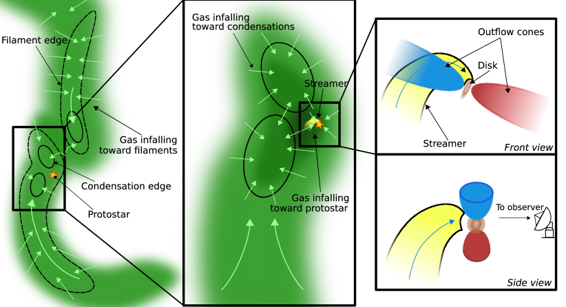
Figure 14: Diagram showing the flows of gas at the different scales investigated in this work. The yellow star indicates the position of the protostar. Left: Infall of fresh gas (green clouds) from B5 dense core toward the filaments (black dashed contours), with the flow direction indicated by the light green arrows. Black solid contours outline the condensations. Center: Infall of fresh gas from the filament toward the condensations (black solid contours) and the protostar, showing the change in direction from the filament to the condensations. The yellow curve shows the streamer transporting material toward the protostellar disk. Top Right: Infall of gas into the protostellar disk (brown disk) through the streamer (yellow flow), which is behind the blue outflow cone (blue cone). The blue arrow indicates the flow direction of the blueshifted streamer. Bottom right: Same as in the top right, but rotated by 90° to observe the streamer unobstructed by the outflow cone.

1. HC3N emission traces the gas flow from the coherent core to the filaments. It is consistently redshifted with respect to the dense gas, observed in NH3, which indicates that it follows different kinematic properties than the dense core tracer. HC3N ($10-9$) shows velocity gradients perpendicular to the filament length, which is consistent with the velocity profile expected from the contraction of a sheet-like cloud forming a filament (Chen et al., 2020a).

2. Using HC3N ($10-9$) and ($8-7$) transitions, we obtain a mean H₂ volume density $n(\mathrm{H}_{2})\approx 10^{5}$ cm^-3. With this value, we estimate that HC3N traces accretion rates of $\dot{m}=4.3\times 10^{-5}$ $\rm M_{\sun}$ yr^-1 in Fil-1 and $\dot{m}=3.5\times 10^{-5}$ $\rm M_{\sun}$ yr^-1 in Fil-2, similar to the accretion rates obtained in previous works which used NH3 emission.

3. We find one streamer and one streamer candidate toward B5-IRS1, using a clustering algorithm on the velocity components found in H2CO emission. We confirm that H2CO emission is mostly unaffected by the outflow cone in this region. We confirm the infalling nature of the clustered component which is blueshifted with respect to the protostar using a streamline model. The categorization of the component that is redshifted with respect to IRS1 is left as tentative as we only traced a small part of this infall. We estimate that the streamer has a total length of around 2800 au through the resulting parameters of the applied streamline model.

4. We sugest that the infall of chemically fresh gas toward the condensations and filaments is connected to the protostar via the streamer. At the location of the protostar, HC3N ($10-9$) central velocities decrease with respect to its surroundings. The location of the blueshift coincides with the location of the streamer and the velocity gradients seen in HC3N coincide in orientation with the velocity gradient shown by the streamer. We suggest HC3N is also sensitive to the infall at small scales, which we know are present because of the high-resolution observations.

Our results highlight the importance of the environment in the comprehension of the physical and chemical processes around protostars. The properties of both the core and the protostellar disk can be affected by the infall mechanisms we observe: there is both chemically fresh gas being deposited toward the filaments, as well as a preferential channel to deposit gas from the envelope to the disk. Intermediate spatial resolution observations are required to confirm the large-scale infall traced using HC3N ($10-9$) with the small-scale infall seen in H2CO emission.

Appendix A Very Large Array and Green Bank Telescope observations

We used the NH3 (1,1) inversion transition data from P15 to define the filaments and cores and compare them to our NOEMA and 30m observations. The details of the reduction can be found in P15 and S21. In summary, VLA observations using the K-band were taken using D and CnD configuration (project number 11B-101), and GBT observations were included to recover the zero-spacing information in the UV plane (project number 08C-088). The data were reduced and imaged using CASA, with multiscale CLEAN and a Briggs weight (robust parameter of 0.5).

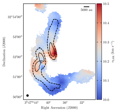
Figure 15: Central velocities of the NH3 (1,1) spectra from P15. The dashed lines outline the filaments seen in NH3 (1,1). The solid lines outline the condensations seen through the same molecule emission. The star marks the position of B5-IRS1.

Figure 1 shows the contours of the dense filaments and condensations found in NH3 (1,1) emission from P15 as defined in S21, which used dendogram analysis to define the filaments and condensations. We use their nomenclature to name the filaments and cores throughout this work. Figure 15 shows the central velocities $\rm\textit{v}_{LSR}$ obtained in P15 from a line fit to the NH3 (1,1) hyperfine components using the cold-ammonia model implemented in pyspeckit (Ginsburg & Mirocha 2011; Ginsburg et al. 2022). The central velocities range from 10 to approximately 10.5 $\rm km\,s^{-1}$ and vary smoothly across the map. The central velocities’ uncertainties are on average $7\times 10^{-5}$ $\rm km\,s^{-1}$ and range from $3\times 10^{-5}$ $\rm km\,s^{-1}$ within the condensations and $2\times 10^{-4}$ $\rm km\,s^{-1}$ at the edges of the filaments. Fil-1 shows a velocity gradient from 10.1 to 10.5 $\rm km\,s^{-1}$ approximately from north to south, and Fil-2, from 10 to 10.3 $\rm km\,s^{-1}$ from south to north, except near the protostar.

Appendix B H2CO moment maps

Figure 16 shows moments 1 (weighted velocity) and 2 (weighted velocity dispersion) for H2CO emission with $S/N>5$. The moment maps show that emission has different velocities in the east-west direction. Emmision toward the east of the protostar has a larger extension and is blueshifted with respect to B5-IRS1’s $\rm\textit{v}_{LSR}$ (10.2 $\rm km\,s^{-1}$, P15, ). Emission toward the west covers less area and is mostly redshifted with respect to the protostar. The moment 1 map shows a curved boundary within a beam of the protostar for the blue and redshifted sides.

The moment 2 map shows that most H_2CO emission has a variance $\sigma^{2}$ of about 0.1 $\rm km\,s^{-1}$, except within a radius of approximately 0$\aas@@fstack{\prime\prime}$5 from the protostar and toward the south of it as well. Most notably, the peak of $\sigma^{2}$ is within a resolved distance (one beam) of B5-IRS1, toward the east.

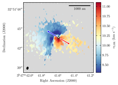
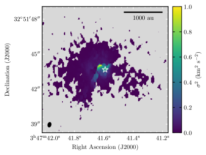
Figure 16: Moments 1 (left) and 2 (right) of the ALMA H2CO ($3_{0,3}-2_{0,2}$) line emission. The black (left) and white (right) stars represent the position of the protostar. The blue and red arrows indicate the directions of the blue and redshifted outflow lobes from Zapata et al. (2014). The scalebars indicate a length of 1000 au. The black ellipse in the bottom left corner represents the beam size.

Appendix C C^18O line emission images

Figure 17 shows the integrated emission of C^18O from 7.8 to 12.4 $\rm km\,s^{-1}$. Figure 18 shows the channel maps of C^18O between 7.8 and 12.3 $\rm km\,s^{-1}$ in 0.3 $\rm km\,s^{-1}$ steps. C^18O traces both the envelope and the natal cloud and is more extended than H2CO. Channels between 9.6 and 10.4 $\rm km\,s^{-1}$ are affected by strong bowls of negative emission due to missing short-spacing data, but C^18O is more affected by the missing scales than H2CO, as it has larger regions with negative emission artifacts. C^18O shows point-like emission between 7.8 and 9.0 $\rm km\,s^{-1}$ and from 11.1 to 12.3 $\rm km\,s^{-1}$, which we suggest comes from the gas disk surrounding the protostar.

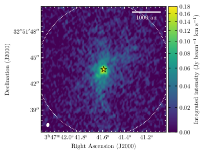
Figure 17: Velocity integrated image of C^18O emission from 7.8 to 12.4 $\rm km\,s^{-1}$. We note that the area covered in the C^18O map is larger than for the H2CO image, shown in Fig. 3. The black star represents the position of the protostar. The scalebar indicates a length of 1000 au. The white ellipse in the bottom left corner represents the beam size. The primary beam of the image is drawn with a white dotted circle.

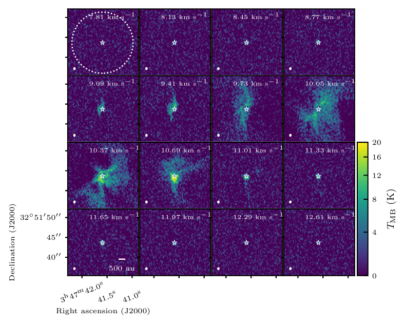
Figure 18: Channel maps between 7.81 and 12.61 $\rm km\,s^{-1}$ for the ALMA C^18O (2 – 1) spectral cube. The white star represents the location of the protostar. The white dotted circle marks the extent of the primary beam. The white ellipse at the bottom left corners represents the beam size. The scalebar shows a 500 au length in the map.

Appendix D Gaussian fit to the spectra and selection criterion

We fit a single Gaussian component to the spectra in the HC3N (10–9) cube and one, two, and three Gaussian components in the H₂CO (3_0,3–2_0,2) cube, using the Python pyspeckit library (Ginsburg & Mirocha 2011). We leave out of the analysis all spectra with a peak S/N lower than 5 for the case of HC3N and lower than 3 for H2CO.

We created a mask with the pixels to fit. First, we select all pixels with $S/N>5$. Then, we did a series of morphological operations on the mask using the morphology library from scikit-image python package (van der Walt et al. 2014). For HC3N we did the following operations in order: first, we removed islands with fewer than 100 pixels using the function remove_small_objects. Secondly, we filled the holes smaller than 100 pixels with the function remove_small_holes. Finally, we did a morphological closing of the mask to fill cracks in the mask, using the closing function with a circular footprint with radius of 6 pixels.

For H2CO, we built the mask with the following sequence: first, we removed islands with fewer than 50 pixels using the function remove_small_objects. Secondly, we filled the holes smaller than 50 pixels with the function remove_small_holes. Then, we did a morphological closing of the mask to soften cracks in the edges, using the closing function with a circular footprint with radius of 3 pixels. Afterwards, we filled the holes with fewer than 200 pixels. Finally, we did a morphological opening of the mask to round the edges using a disk footprint of radius 4 pixels. This mask allowed us to capture pixels with significant H2CO emission, larger than $S/N>3$, that are connected to significant areas of emission and not in disconnected islands that are associated to artifacts.

The initial guesses are fundamental in all of our fits to obtain reasonable results. For HC3N, we first obtained the moments of the cube, as described in the Minimal Gaussian cube fitting example from pyspeckit. Then, we checked the initial guesses to replace any value that is not within acceptable ranges, as follows. If the initial peak is negative, we replace it with a value of 0 K. If the initial central value was not within the range of observed velocities (between 9 and 11.3 $\rm km\,s^{-1}$), we replaced it with 9 $\rm km\,s^{-1}$ if the value was lower than 9 $\rm km\,s^{-1}$ and with 11.3 $\rm km\,s^{-1}$ if the value was higher than 11.3 $\rm km\,s^{-1}$. We replaced all initial velocity dispersions larger than 2.3 $\rm km\,s^{-1}$ to 2.3 $\rm km\,s^{-1}$, which is the difference between the observed velocity boundaries. In the pixels where the initial guesses were not a number (NaN), we replaced the peak intensity for 1 K, the central velocity for 10.2 $\rm km\,s^{-1}$ and the dispersion for 1 $\rm km\,s^{-1}$.

The initial guesses for H2CO fit were different in the cases we fit one, two and three Gaussians. For one Gaussian, we used the same initial guesses for all pixels: a peak temperature $T_{\mathrm{peak}}$ of 10 K, central velocity $\rm\textit{v}_{LSR}$ of 10.2 $\rm km\,s^{-1}$ and dispersion $\sigma_{\mathrm{v}}$ of 0.8 $\rm km\,s^{-1}$. For two Gaussians, we use the same initial guesses for most of the pixels except for select regions where we input different guesses manually. For most of the pixels, the first component had initial guesses of $T_{\mathrm{peak}}=10$ K, $v_{\mathrm{LSR}}=10.5$ $\rm km\,s^{-1}$ and $\sigma_{\mathrm{v}}=0.3$ $\rm km\,s^{-1}$, and the second, $T_{\mathrm{peak}}=10$ K, $v_{\mathrm{LSR}}=9.2$ $\rm km\,s^{-1}$ and $\sigma_{\mathrm{v}}=0.3$ $\rm km\,s^{-1}$. For three Gaussians, our initial guesses were $T_{\mathrm{peak}}=10$ K, $v_{\mathrm{LSR}}=11.3$ $\rm km\,s^{-1}$ and $\sigma_{\mathrm{v}}=0.3$ $\rm km\,s^{-1}$ for the first component, $T_{\mathrm{peak}}=10$ K, $v_{\mathrm{LSR}}=10.7$ $\rm km\,s^{-1}$ and $\sigma_{\mathrm{v}}=0.3$ $\rm km\,s^{-1}$ for the second, and $T_{\mathrm{peak}}=5$ K, $v_{\mathrm{LSR}}=9.5$ $\rm km\,s^{-1}$ and $\sigma_{\mathrm{v}}=0.3$ $\rm km\,s^{-1}$ for the third, except for selected regions where we input different guesses manually.

After fitting once, we did a second fit, using the resulting output from the first fit as initial guesses. To do this, we selected for further analysis the fitted spectra that met all of the following requirements and the rest are replaced with NaNs: the parameter uncertainties had to be all smaller than 50%; the amplitude of the Gaussian was a positive value; the Gaussian component had a central velocity in the observed emission velocity range (between 8 and 12 $\rm km\,s^{-1}$ for H₂CO, and between 9 and 11.3 $\rm km\,s^{-1}$ for HC3N); and finally, the fitted amplitude had $S/N>2$ for the case of H2CO and $S/N>5$ for HC3N. Then, we interpolated the parameters obtained that passed this filter to fill in the pixels where the fit did not converge to a solution with the initial guesses, or where the first fit did not pass the filter described above. For the interpolation we used the griddata function from the scipy.interpolate python library (Virtanen et al. 2020). Afterwards, we input the interpolated values as initial guesses for the fits.

To mitigate the effects of the missing short- and zero-spacing information in our interferometric data for the H2CO fit, we fit one, two and three Gaussian components using the spectra with the values between 9.7 and 10.3 $\rm km\,s^{-1}$ masked, following the same procedure above. This only has a positive net effect on the final results for the spectra within a 500 au radius from the protostar. For the rest of the spectra, masking the channels has no net positive effect on the final results and misses Gaussian components that peak within the masked channels. Therefore, we only used the fit with masked central channels for the spectra within a 500 au radius.

We kept the second fit results and did a further quality assessment. For HC3N, the assessment included the requirements mentioned above. For H2CO, we added the following criteria after evaluating the previous requirements: first, the fitted amplitudes selected all had $S/N>3$; the uncertainty in the central velocity for each fit had to be less than the channel size (0.08 $\rm km\,s^{-1}$ for the H2CO ALMA cube, Table 1); and finally, for pixels where the fit was done with masked channels, there could not be a peak located at the masked channels. After this evaluation, we also filtered islands of pixels in the image space that had fewer than 50 pixels for the one Gaussian fit, and fewer than 15 pixels for the two Gaussian fitting, as this would only add noise to the clustering.

We used the Akaike information criterion (AIC) to decide how many Gaussian components reproduced best each spectra, in a similar manner as applied in Choudhury et al. (2020) and Valdivia-Mena et al. (2022), for the case where we fit up to 3 Gaussians in H2CO. This criterion uses the AIC value $AIC$ to determine which model minimizes information loss:

$$AIC=2k+\chi^{2}+C,$$ (2)

where $k$ is the number of free parameters of the model, $\chi^{2}$ is the classical chi-squared statistic and C is a constant defined by the number of independent channels and the uncertainties (Choudhury et al. 2020). Because each Gaussian component has three free parameters, $k=3g$, where $g$ is the number of Gaussian components in each model. For $C$, we assumed that each channel in the spectra has a constant normal error, which corresponds to the rms of each cube. As we used the same data to test the three models, C is the same for all models and does not play a role in choosing the best, so we set $C=0$.

We evaluated the probability that the model with the minimum information loss, which is the one with the minimum $AIC$, is a considerable improvement from the other models for each spectrum. The probability that model $i$ is as good as the model with minimum $AIC$ to minimize information loss is proportional to the differencce between the minimum AIC, $AIC_{min}$ and the AIC value of model i, $AIC_{i}$:

$$P=\exp\Big{(}\frac{AIC_{min}-AIC_{i}}{2}\Big{)}.$$ (3)

For each spectrum, the fit with the lowest AIC value is the preferred one. We also checked that the best fit has at least a 95% probability of minimizing the information loss better than when compared with any other of the models applied: this translates to a value of $P<0.05$. For the case of H2CO, there are very few spectra (around 0.1%) where the probability is less than 95% for the best model, so we leave the fit with the lowest AIC value.

D.1 HC3N two Gaussian fit

The best fit parameters for the HC3N emission spectra are in Figure 5. Figure 19 shows the spectrum at the position of the protostar and its Gaussian fit with a dashed line. We also did a two Gaussian fit to the central 4″around the protostar in the HC3N map. This possible second feature is hinted at in the residuals of the one Gaussian fit at the position of the protostar, seen in Fig. 19, where some residuals reach $S/N\gtrsim 3$. We fit two Gaussians and compare the results using the Akaike Information Criterion (AIC). The resulting fit at the location of the protostar is shown in Fig. 19 with solid lines. The residuals from both fits show that two Gaussians fit the spectrum better than one at the position of the protostar. However, as too few spectra were actually better fitted with two Gaussians that with one when evaluated with AIC (less than 10% of the pixels, Fig. 20), we decided to leave all spectra with only one Gaussian.

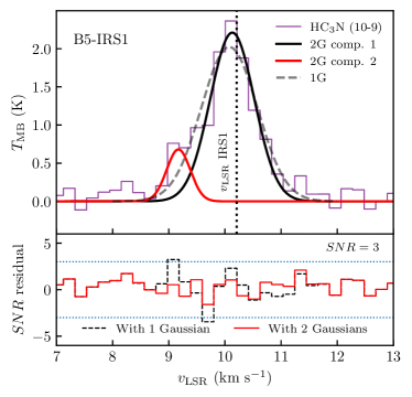
Figure 19: Results from the one- and two-Gaussian fit to the HC3N (10–9) emission at the position of the protostar B5-IRS1. Top: HC3N (10–9) emission spectrum at the position of B5-IRS1, together with the best fit results using one and two Gaussian curves. The vertical dashed line represents the central velocity of the protostar from P15. Bottom: residuals from the fit in terms of $S/N$. The dashed purple line represents the residuals after the 1 Gaussian fit, whereas the solid purple line, the residuals after the 2 Gaussian fit. The horizontal blue dashed lines mark the $S/N=3$ and $-3$ levels.

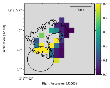
Figure 20: Probability $P$ (Eq. 3) for two Gaussian components fit in HC3N (10–9) around 4″from the protostar. Contours indicate the location of the blue streamer found in Sect. 4.2.1.

Appendix E Core and filament volume density traced by HC3N

We obtained the volume density of H2 gas $n(H_{2})$ using the HC3N line ratio between the 10 – 9 and 8 – 7 level transitions and the non-LTE radiative transfer code RADEX (van der Tak et al. 2007), with the goal of calculating the infall rate of material from the core to the filaments in Barnard 5.

E.1 HC3N (8 – 7) integrated image

Figure 21 shows the integrated intensity of HC3N $(8-7)$ emission. We integrated the line cube between 9.2 and 11.2 $\rm km\,s^{-1}$, the same range as for HC3N $(10-9)$. The morphology is similar to the HC3N $(10-9)$ integrated map, but the peak in integrated intensity is located within Cond-2 instead of the protostar.

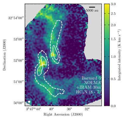
Figure 21: Velocity integrated HC3N $(8-7)$ line emission, from 9.2 to 11.2 $\rm km\,s^{-1}$. White dashed contours correspond to the filaments identified in NH3 emission by P15 and S21. White solid contours outline the edges of the condensations labeled as in P15. The gray star marks the position of the protostar B5-IRS1.

E.2 HC3N line ratio

We used the integrated line intensity maps for both HC3N transitions to obtain a line ratio map. First, we smoothed the HC3N ($10-9$) integrated image with a Gaussian kernel in CASA to the reach the resolution of the ($8-7$) transition map ($\approx 5\arcsec$, Table 1). Then, we regridded the resulting convolved image to match the ($8-7$) line map pixel grid. Finally, we divided the regrid HC3N ($10-9$) integrated intensity map by the HC3N ($8-7$) integrated image:

$$R_{\frac{10-9}{8-7}}=\frac{\int T_{R,10-9}dv}{\int T_{R,8-7}dv},$$ (4)

where $\int T_{R}dv$ is the integrated intensity of a spectrum in K $\rm km\,s^{-1}$. The resulting map is in Fig. 22 and includes pixels where $S/N>5$ for both $10-9$ and $8-7$ transitions.

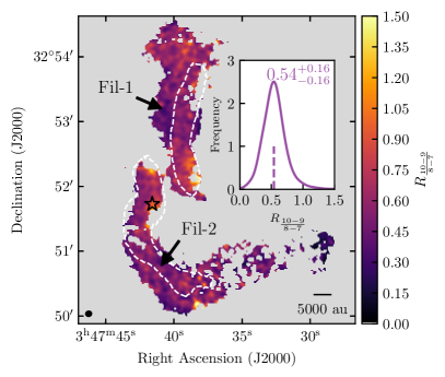
Figure 22: Map of the line ratio between the HC3N ($10-9$) and (8 – 7) transitions. White dashed contours correspond to the filaments identified in NH3 emission by P15 and S21. The black star marks the position of the protostar B5-IRS1. Inset: KDE of the line ratios obtained. The dashed vertical line shows the median value of the distribution, and the uncertainties correspond to the distance to the 1st and 3rd quartiles.

In general, $R_{\frac{10-9}{8-7}}$ does not present large systematic variations along the filaments, and variations are usually clumpy and reach differences of up to 0.2 within one beam. The distribution of line ratios of the whole map is shown in the inset of Fig. 22: it has a median of 0.54 and its shape resembles a Gaussian. The ratio does reach values up to 1.0 in the vicinity of the protostar, which could occur due to higher temperatures and/or higher optical thickness in the region. Very low values of $R_{\frac{10-9}{8-7}}$, under 0.2, and very high values, over 1.1, are located in the edges of the filaments and are due to the detection edges of either HC3N ($10-9$) or HC3N ($8-7$). Near the condensations the ratio is also slightly higher, increasing from $\approx 0.55$ to $\approx 0.65$. This could be due to a higher temperature closer to the condensation, caused by mass infall, which would then populate more the ($10-9$) transition, and/or emission in the condensations becoming optically thick. As the map shows no considerable spatial variations, it is safe to take its mean to describe the volume density of the whole emission.

E.3 H2 volume density traced by HC3N

We took the mean value of the distribution, $<R>=0.56\pm 0.01$, to estimate the H₂ density $n(H_{2})$ and the excitation temperature $T_{ex}$ for the HC3N ($10-9$) transition. We compared this ratio with the results from the RADEX models run by Pineda et al. (2020), as their input parameters result in similar emission intensities $T_{R}$ as the ones observed in this work and the line ratios resulting from their test (between 0.2 and 0.8) include our resulting line ratio. A line ratio $<R>=0.56\pm 0.01$ corresponds to a density of $\approx 10^{5}$ cm^-3 (based on the Extended data fig. 1 from Pineda et al. (2020)) and results in an excitation temperature $T_{ex}\approx 6.4$ K for the $10-9$ molecular transition.

Appendix F Clustering of H2CO Gaussian components

We clustered the different Gaussian components found in Sect. 3.4 to aid in their physical interpretation. We applied the unsupervised learning tools from the scikit-learn Python library (Pedregosa et al. 2011) to the results of our 1, 2 and 3 Gaussian component fitting of the ALMA H2CO emission. We used the right ascension (RA), the declination (DEC) and central velocities ($\rm\textit{v}_{LSR}$) of each Gaussian component as features for clustering. Using all properties of the fits as features, or using the three mentioned parameters plus either amplitude or velocity dispersion, does not represent an improvement in the clustering of the Gaussian components. We first scaled all the features to a range from -1 to 1 using the StandardScaler class in the preprocessing Python library. By doing so, we assigned the same relative weight to all the features. Then, we used the algorithm DBSCAN (Ester et al. 1996), implemented in the DBSCAN class, with parameters eps $=0.248$ and min_samples $=100$. The rest of the parameters are left as default. This results in 5 clusters in (RA, DEC, $\rm\textit{v}_{LSR}$) space. The resulting groups found by DBSCAN are shown in Fig. 23.

There are a total of 11992 individual Gaussian components in the cube, out of which DBSCAN determined 3042 (25%) are outliers, and do not belong to any cluster. This does not imply that these Gaussians are fitting noise, only that the features could not be grouped. In particular, points within 1″to the east of the protostar could not be grouped. This region is dominated by emission with $\rm\textit{v}_{LSR}$ $\approx 9.25$ $\rm km\,s^{-1}$. We suggest this emission is also part of the blueshifted streamer described in Sect. 4.2.2, as it follows the same apparent gradient. Adding these points to the blueshifted cluster does not affect the streamline model nor the resulting centrifugal radius, so we decided to follow the grouping resulting from the clustering algoithm. Out of all the clustered points, the largest group is a fully blueshifted cluster (consisting of 5529 individual points) and the second largest, a fully redshifted cluster (with 2557 individual points), with respect to the protostar’s $\rm\textit{v}_{LSR}$ (10.2 $\rm km\,s^{-1}$).

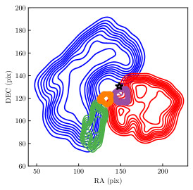
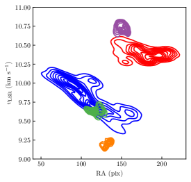
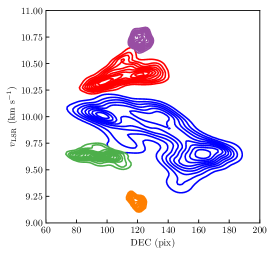
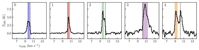
Figure 23: Results from the clustering of the Gaussian components in the ALMA H2CO spectra. Each cluster is labeled with a number from 0 to 4, in order of descending number of points. Blue and red points (labeled 0 and 1) represent the clusters named blueshifted and redshifted component, respectively. Orange, purple and green points represent the other three found clusters. Top: Density plots of the clustered groups using Gaussian KDEs, seen in the image plane (RA and DEC in pixels, left), in RA versus $\rm\textit{v}_{LSR}$ (middle) and in DEC versus $\rm\textit{v}_{LSR}$ (right). The black star marks the position of the protostar. Bottom: average spectra taken from the area covered by each group, labeled with the numbers from the Top Left panel. The ALMA H2CO spectra are drawn with black solid lines. The colored vertical areas represent the location of average $\rm\textit{v}_{LSR}$ and FWHM of each cluster. The vertical dotted line marks the protostar’s $\rm\textit{v}_{LSR}$.

F.1 Nonthermal velocity dispersion of H2CO emission

We checked the velocity dispersion $\sigma_{\mathrm{v,fit}}$ of the Gaussians in the blueshifted and redshifted clusters and compared them to the thermal sound speed. Nonthermal velocity dispersion larger than the sound speed can be attributed to the outflow or to gas tracing rotation motions instead of infall.

First, we deconvolved the velocity dispersion with respect to the channel size of our data using

$$\sigma_{\mathrm{v}}^{2}=\sigma_{\mathrm{v,\,fit}}^{2}-\frac{2\Delta_{\mathrm{ch}}}{2.355},$$ (5)

where $\Delta_{\mathrm{ch}}$ is the channel width (Table 1). Then, we subtracted in quadrature the thermal dispersion $\sigma_{\mathrm{th}}$ from the deconvolved velocity dispersion, thus obtaining $\sigma_{\mathrm{v,\,nt}}$:

$$\sigma_{\mathrm{v,\,nt}}^{2}=\sigma_{\mathrm{v}}^{2}-\sigma_{\mathrm{th}}^{2}.$$ (6)

The thermal dispersion is

$$\sigma_{\mathrm{th}}=\sqrt{\frac{k_{B}T}{\mu_{\mathrm{H}_{2}\mathrm{CO}}m_{\mathrm{H}}}}=0.052\,\mathrm{km\,s}^{-1},$$ (7)

where $k_{B}$ is the Boltzman constant, $T$ is the kinetic temperature of the gas, which we assumed is 9.7 K from Pineda et al. (2021), $\mu_{\mathrm{H}_{2}\mathrm{CO}}=30.026$ is the molecular weight of the H2CO molecule and $m_{\mathrm{H}}$ is the mass of a Hydrogen atom.

The resulting $\sigma_{\mathrm{v,\,nt}}$ for the two envelope components are in Fig. 24. The dispersion increases when the distance to the protostar decreases for both components, but it is mostly subsonic for both parts of the envelope. H2CO emission becomes transonic (larger than $c_{\mathrm{s}}=0.18$ $\rm km\,s^{-1}$) within $r\lesssim 600$ au approximately. This means that, for majority of the emission within both components, the H2CO gas is unaffected by the outflow and is not caused by Keplerian rotation.

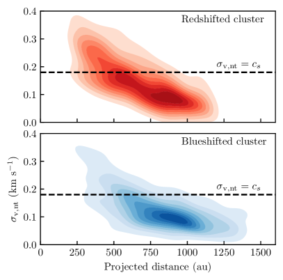
Figure 24: KDE of the nonthermal velocity dispersion for the blueshifted and redshifted envelopes. The dashed line represents where $\sigma_{\mathrm{v,\,nt}}$ equals the sound speed for gas at 9.7 K (0.18 $\rm km\,s^{-1}$).

Appendix G Estimate of the protostellar mass

We used the C^18O ($2-1$) ALMA data to estimate the protostellar mass of B5-IRS1. We first looked at the position-velocity (PV) diagram of C^18O using the astropy package pvextractor (Ginsburg et al. 2016). We generated the PV diagram along a path centered on the protostar with a total length of 1600 au, with a position angle (PA) of 157$\aas@@fstack{\circ}$1 (with 0°  pointing toward the north), obtained from the outflow PA (Zapata et al. 2014), and a width of 0$\aas@@fstack{\prime\prime}$4. The pixel size of the C^18O cube is 0$\aas@@fstack{\prime\prime}$054, so we chose to take an integer number of pixels as the width of the PV sampling path that was as close to the beam width as possible (7 pixels, or 0$\aas@@fstack{\prime\prime}$4). The resulting PV diagram is in Fig. 25 and shows the classical diamond shape that is attributed to a combination of Keplerian rotation and infall motion of the inner envelope (e.g., Lee et al. 2014; Sakai et al. 2014). When we compare the PV diagram with the Keplerian curve produced by a 0.1 $\rm M_{\sun}$ protostellar mass (the previously reported protostellar mass in Brassfield & Bourke 2011) and for a disk with an inclination $i=77\degr$ (obtained from the outflow inclination angle $i=13\degr$, Yu et al. 1999), the PV diagram 5$\sigma$ limit is above the curve, indicating the protostar’s mass is possibly higher. We plotted over the PV diagram the Keplerian curve for 0.2 $\rm M_{\sun}$ with the same disk $i$ and we saw that it is closer to the 5$\sigma$ edge than 0.1 $\rm M_{\sun}$. From this simple observation, we suspect the central protostar’s mass is be higher. To confirm, we did a deeper analysis into the C^18O data.

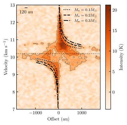
Figure 25: Position-velocity diagram of the ALMA C^18O datacube, centered at the position of the protostar, with a PA of 157$\aas@@fstack{\circ}$1 and a width of 0$\aas@@fstack{\prime\prime}$4. The black curves show the Keplerian rotation profile produced by three protostellar massses: the dotted line shows the Keplerian curve for a protostar of 0.1 $\rm M_{\sun}$ (Brassfield & Bourke 2011), the dashed line for 0.2 $\rm M_{\sun}$, and the dash-dotted line for 0.3 $\rm M_{\sun}$. The dotted horizontal line marks the protostar’s $v_{\mathrm{LSR}}=10.2$ $\rm km\,s^{-1}$. The scalebar represents one beam width (120 au or 0$\aas@@fstack{\prime\prime}$4)

We obtained the central position of C^18O emission in each velocity channel and determine if it is consistent with Keplerian motion. For this, we fit a two-dimensional Gaussian at each of the channels of the C^18O ($2-1$) cube between 7.9 and 9.2 $\rm km\,s^{-1}$ and between 10.8 and 12.4 $\rm km\,s^{-1}$. These ranges cover the velocities of C^18O emission that are the most blueshifted and redshifted with respect to the protostar, and miss the central channels seen in Fig.  18, where emission is affected by missing short- and zero-spacings. We used the models.Gaussian2D class and fit the Gaussian model using least-squares minimization with the Levenberg-Marquardt algorithm, implemented in the fitting.LevMarLSQFitter class. Both classes are part of the astropy python package. We use the peak value of each channel, the position of the peak, and the beam width $\sigma_{\mathrm{beam}}=\theta_{\mathrm{FWHM}}/2.355$ (Table 1) as initial guesses for the amplitude, central position and dispersion of the Gaussian at each channel. We used the channels between $v_{\mathrm{LSR}}=7.9-8.8$ $\rm km\,s^{-1}$ and $11.1-12.4$ $\rm km\,s^{-1}$ to calculate the barycenter (i.e. the rotation center) of the points blueshifted and redshifted with respect to the protostar’s $v_{\mathrm{LSR}}$. Finally, we calculated the distance of each point to the calculated barycenter $d$ and plot $d$ against the corresponding channel’s velocity with respect to the protostar’s $v_{\mathrm{LSR}}$, $\delta v_{\mathrm{LSR,IRS1}}=v_{LSR}-10.2$ $\rm km\,s^{-1}$. Using the corrected center instead of the position from Tobin et al. (2016) returns a more precise velocity versus distance plot. Nevertheless, the distance between the barycenter and the protostar’s coordinates is $\lessapprox 0\aas@@fstack{\prime\prime}1$.

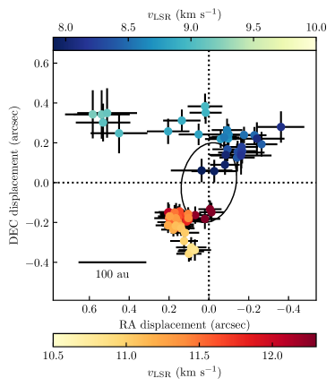
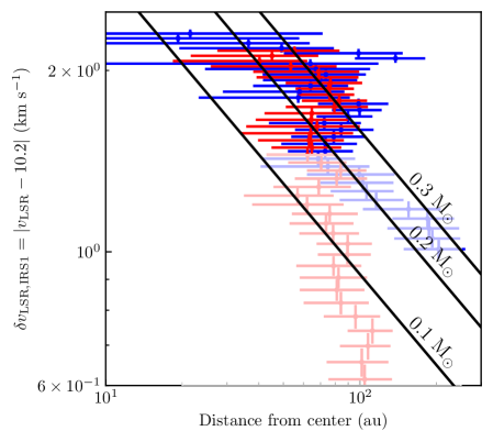
Figure 26: Results from the two-dimensional Gaussian fit to the C^18O channel maps. Left: Best fit central positions with respect to the image plane, where their colors represent the velocity of the channel $\rm\textit{v}_{LSR}$. The dashed lines represent the position of the barycenter. The ellipse centered at the barycenter represents the beam size (FWHM). Right: C^18O emission velocity with respect to the protostar’s $\rm\textit{v}_{LSR}$ versus distance from the protostar. Blue dots are obtained from the C^18O emission blueshifted with respect to the protostar and red dots from the redshifted emission. Faded dots come from velocity channels with considerable extended emission, and therefore their properties are affected by motions other than Keplerian. The solid black lines are the Keplerian rotation profiles for 0.1, 0.2 and 0.3 $\rm M_{\sun}$.

The resulting C^18O central positions per velocity channel are in Fig. 26 Left and the velocity versus distance plot is in Fig. 26 Right. The faded blue and red points represent the fitted positions where there is extended emission in the velocity channel, which affected the Gaussian fit. For emission peaks located from 0 to about 70 au (0$\aas@@fstack{\prime\prime}$2), as distance from the protostar increases, $\delta\mathrm{v}_{LSR,\mathrm{IRS1}}$ tends to decrease. In the image plane, as $\delta\mathrm{v}_{LSR,\mathrm{IRS1}}$ decreases, the points tend to get away from the protostar in opposite directions along a northwest to southeast orientation, similar to the orientation of the disk used to obtain the PV diagram. These two behaviors are expected for Keplerian rotation. However, emission centered farther away than $\sim 70$ au show a change in direction: as $\rm\textit{v}_{LSR}$ gets closer to the protostar’s $\rm\textit{v}_{LSR}$, the blueshifted points move toward the east instead of northwest, and the redshifted points move toward the west instead of southeast. These low $\delta\mathrm{v}_{LSR,\mathrm{IRS1}}$ “tails” have different behaviors in velocity versus distance: $\delta\mathrm{v}_{LSR,\mathrm{IRS1}}$ drops faster with distance for the redshifted points than for the blueshifted ones. Moreover, the blueshifted and redshifted points that are the farthest away from the protostar are at the edges of the blueshifted and redshifted envelope components, respectively. We note that these points come from the channels which have considerable extended emission. This suggest that C^18O emission is tracing part of the infall that we trace with H2CO emission as C^18O extended emission.

We plotted the Keplerian velocity versus distance curve expected for a protostellar mass of 0.1, 0.2 and 0.3 $\rm M_{\sun}$ over the velocity versus distance plot for C^18O positions (in Fig. 26 Right). The uncertainty in central position is too large to fit a Keplerian rotation curve to these data, so we only overplot the expected Keplerian curves for the selected masses and do not attempt to obtain a radius from these data points. Most of the points less than 100 au away from the protostar fall between the 0.2 and 0.3 $\rm M_{\sun}$ curves. However, the large uncertainty of the points that are closer to the protostar are too large to clearly distinguish between both cases, some also reaching values consistent with 0.1 $\rm M_{\sun}$. We decide to use a protostellar mass of 0.2 $\rm M_{\sun}$, as this is not far from the value presented in Brassfield & Bourke (2011) but still looks consistent with most of the points obtained from our Gaussian fit and the 5$\sigma$ contours of the PV diagram (Fig. 25).

Appendix H Comparison between H2CO and H^13CO+

We compared the emission coming from the blueshifted component from the DBSCAN analysis (Sect. 4.2.1) with the H^13CO+ emission from van’t Hoff et al. (2022) both in the image plane and in velocity space. We first looked at the location of emission. van’t Hoff et al. (2022) show that H^13CO+ emission has a ridge-like shape toward the west of B5-IRS1. H^13CO+ peak emission ridge coincides with the area occupied by the blueshifted component, although emission with $S/N>3$ is more extended than the blue streamer. Spatial coincidence does not mean both molecules trace the same part of the envelope, so we looked into the kinematics of H^13CO+.

We fit a Gaussian curve to the H^13CO+ spectra with the same procedure as for HC3N (Appendix D) but first selecting all spectra with $S/N>3$ to make the mask. The resulting central velocities are in Fig. 27 Left. We note that all the velocities in the east side of B5-IRS1 are blueshifted with respect to the protostar. H^13CO+ shows a velocity gradient from 10.1 to 9.4 $\rm km\,s^{-1}$ as distance to the protostar decreases. This gradient is similar to the gradient seen in the blueshifted component in Fig. 11, which suggest both molecules trace an infall motion. This also confirms that H^13CO+ does not trace outflow motion, using the same arguments as in Sect. 4.2.2.

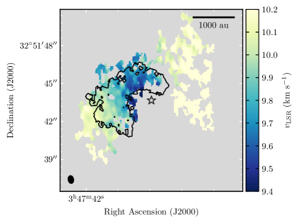
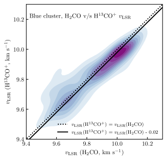
Figure 27: Comparison between the $\rm\textit{v}_{LSR}$ found for H^13CO+ observations from van’t Hoff et al. (2022) and our H2CO $\rm\textit{v}_{LSR}$ results. Left: Central velocities obtained through the Gaussian fit to H^13CO+ observations from van’t Hoff et al. (2022). The black ellipse represents the beam size. The black contour indicates the area covered by the H2CO blueshifted cluster found using DBSCAN. The black star represents the position of B5-IRS1. Right: KDE of the difference between the central velocities of H2CO and H^13CO+ emission. The dotted line shows the one-to-one relation, and the solid line shows the same relation but displaced by 0.02 $\rm km\,s^{-1}$

We calculated the difference between $\rm\textit{v}_{LSR}$ for H2CO and H^13CO+ spectra to investigate if H2CO has any additional movement with respect to H^13CO+ or if differences are random. For this, we reprojected the spatial grid of H2CO to the one of H^13CO+ using the astropy package reproject. The KDE of the difference is in Fig. 27 Right. Differences in velocity appear to be random; there appears to be no tendency for a preferential redshift of blueshift of H2CO with respect to H^13CO+ for any velocity. The median value of the difference is $0.02^{+0.07}_{-0.09}$ $\rm km\,s^{-1}$, smaller than the channel width for H2CO data (Table 1). This means both molecules share the same velocities and velocity gradients. We therefore conclude that both H2CO and H^13CO+ trace the infall motion of the blueshifted streamer.