Effective-Hamiltonian theory: An approximation to the equilibrium state of open quantum systems

Abstract

We extend and benchmark the recently-developed Effective-Hamiltonian (EFFH) method [PRX Quantum 4, 020307 (2023)] as an approximation to the equilibrium state (“mean-force Gibbs state”) of a quantum system at strong coupling to a thermal bath. The EFFH method is an approximate framework. Through a combination of the reaction-coordinate mapping, a polaron transformation and a controlled truncation, it imprints the system-bath coupling parameters into the system’s Hamiltonian. First, we develop a variational EFFH technique. In this method, system’s parameters are renormalized by both the system-bath coupling parameters (as in the original EFFH approach) and the bath’s temperature. Second, adopting the generalized spin-boson model, we benchmark the equilibrium state from the EFFH treatment against numerically-exact simulations and demonstrate a good agreement for both polarization and coherences using the Brownian spectral function. Third, we contrast the (normal and variational) EFFH approach with the familiar (normal and variational) polaron treatment. We show that the two methods predict a similar structure for the equilibrium state, albeit the EFFH approach offers the advantage of simpler calculations and closed-form analytical results. Altogether, we argue that for temperatures comparable to the system’s frequencies, the EFFH methodology provides a good approximation for the mean-force Gibbs state in the full range of system-bath coupling, from ultraweak to ultrastrong.

I Introduction

As an emerging field, strong-coupling thermodynamics aims to expand conventional thermodynamics to account for the impact of the interaction energy between a quantum system and its surroundings on dynamical and thermodynamical processes BookQT . Strong coupling effects may play a crucial role in determining the behavior of various quantum thermal machines such as heat diodes diodeSC0 ; diodeSC1 ; diodeSC2 ; diodeSC3 , thermal transistors transSC1 , engines Brandes ; engineSC ; Marti:2018Engine and refrigerators RefSC1 ; RefSC2 ; RefSC3 ; references here are only examples of a rich literature. Similarly, in complex structures such as light-harvesting systems, the interaction between electronic excitations and the protein complex reveals distinct dynamics compared to the weak coupling regime lphotoSC .

However, prior to delving into the exploration of the nonequilibrium functionality of quantum thermal machines, we encounter a fundamental question concerning the equilibrium (long-time) state of a stationary system when it is coupled to a heat bath. This equilibrium state, referred to as the mean-force Gibbs state (MFGS) represents the reduced state of the overall system when traced over environmental degrees of freedom, see Refs. Hu:2012Eq ; Lutz:2011Eq ; JanetPRL ; Keeling2022 ; JanetQC23 for some recent works. Classically, the Gibbs state is commonly accepted as the equilibrium state of a system interacting with a thermal environment. However, when the interaction between the system and the heat bath cannot be neglected, the state of the system is going to deviate from this conventional state JanetRev .

Various methods have been developed to examine the equilibration dynamics and steady state behavior of open quantum systems, going beyond the weak coupling assumption. These methods can be broadly classified into two categories: numerically-exact methods; such as the Hierarchical Equations of Motion (HEOM) TanimuraHEOM ; Kawai2020 , path integral implementations TEMPO ; Keeling2022 , Monte Carlo methods Guy , generalizations of trace estimators and Krylov subspace methods Cheng2022 , and approximate-perturbative techniques JanetPRL ; Hu:2012Eq ; Lutz:2011Eq ; JanetRev ; JanetQC23 ; Thoss:2009 ; Ahsan14 ; Brumer20 ; Silbey ; ReichS ; Cao1 ; Cao2 ; Cao3 ; LatunePRE ; LatuneMFGS22 ; Valkunas20 ; Becker:2022PRL ; Thingna:2012JCP ; Thingna:2014JCP ; Tupkary:2023PRA ; Lee:2022PRE ; Correa:2023Shift ; Becker:2021PRE ; HanggiRev ; Miller ; Zhang_2022 ; Giacomo that are commonly developed based on the quantum master equation (QME) formalism Nitzan ; Breuer .

In a recent study PRXRC , we introduced a reaction-coordinate polaron-transform framework that enables the analytical and numerical study of strong-coupling thermodynamics problems. By employing two exact transformations of the Hamiltonian followed by a controlled truncation, this approach generates an Effective Hamiltonian (EFFH). This new Hamiltonian resembles the original Hamiltonian, with the dimensionality of the Hilbert space being identical to the starting one, but with dressed parameters that depend on the system-bath coupling parameters.

The essence of the EFFH approach is that strong-coupling effects are directly embedded in the system’s effective Hamiltonian, which after the transformations and truncation can become weakly coupled to the (residual) surroundings, thus allowing applications of weak-coupling techniques to study the resulting dynamics and steady state. Altogether, as demonstrated in Ref. PRXRC , the EFFH method allows a direct and easy analysis of strong-coupling effects. It also provides a route for performing numerical simulations that include strong-coupling effects nonperturbatively—at the cost of a weak-coupling treatment.

The EFFH method was exercised in Ref. PRXRC on several canonical problems, including models for quantum thermalization and charge, spin, and energy transport at the nanoscale. Specifically, it was proposed in Ref. PRXRC that the effective Hamiltonian of the system can be regarded as the Hamiltonian of mean force (HMF) HanggiRev ; Miller . This supposition was supported by demonstrating that a Gibbs state constructed from the system’s EFFH was in fact the exact equilibrium state for the spin-boson model at both the ultraweak and ultrastrong coupling limits JanetPRL . Furthermore, in the intermediate system-bath coupling regime the equilibrium state constructed by the EFFH method agreed qualitatively with the state achieved using the numerical reaction coordinate simulation method.

The analysis in Ref. PRXRC was yet limited in several ways: First, the equilibrium state of the EFFH was not tested against independent tools, specifically numerically-exact approaches. Second, while the generated EFFH of the system depends on the system-bath coupling parameters, it does not depend on the bath’s temperature, contrary to other approaches, specifically the polaron technique Silbey ; Cao1 ; Cao2 ; Cao3 . Furthering the development of the EFFH mapping to cover broader regimes of parameters is necessary. Third, the polaron transform Cao1 ; Cao2 ; Cao3 ; Legget is an established tool for calculating the MFGS of open quantum systems. A relationship between the EFFH method and the standard-popular polaron-frame technique should be established.

The objective of this study is to develop the Effective-Hamiltonian theory and test its viability as a tool for describing the MFGS of open quantum systems, encompassing the full spectrum of system-bath coupling; the ultraweak, intermediate and strong regimes. We contribute the following:

1. Benchmarking: Using the spin-boson model as a case study, we benchmark the EFFH predictions against other methods. Particularly, we show that for a Brownian spectral function EFFH results well agree with numerically-exact simulations at arbitrary coupling, a striking result given that the EFFH state is constructed effortlessly.

2. Extending range of applicability: We extend the Effective Hamiltonian method by introducing a variational optimization to the mapping. As a result, the renormalized parameters of the system become dependent on both the spectral properties of the bath and its temperature. Importantly, the variational effective Hamiltonian (var-EFFH) approach does not require the strict separation of energy scales between a small system splittings ($\Delta$) and a large bath characteristic frequency $\Omega$, so long as the coupling energy is weak-to-intermediate.

3. Contrasting: We study in details the relationship between the MFGS as constructed by the EFFH method and the polaron-transformed approach, particularly, the variational flavors of both tools. We show that both the EFFH method and the polaron approach expose analogous physical effects, such as dressing of the system’s parameters. However, the EFFH framework offers a clear advantage with the simplicity of its derivation and it catering closed-form expressions for the MFGS.

Beyond the spin-boson model, we further reinforce the applicability of the EFFH framework by applying it onto a fully harmonic model.

The paper is organized as follows. In Sec. II we introduce the research question and the principles of the “normal” EFFH method. We further provide benchmarking against numerically-exact simulations. In Sec. III we introduce the principles of the variational EFFH method. A comparative analysis between the EFFH technique and the polaron-transformed approach is provided in Sec. IV. Analytical results for the MFGS and the spin expectation values are given in Sec. V, further presenting extensive numerical simulations in Sec. VI. We conclude in Sec. VII.

II Research question and the EFFH method

We start by presenting the MFGS in general terms. We then provide an overview of the EFFH technique of Ref. PRXRC and introduce the model we use throughout.

II.1 The MFGS

We focus on open quantum systems described by a system’s Hamiltonian $\hat{H}_{S}$ coupled to a reservoir including a collection of harmonic oscillators. The total Hamiltonian comprising the system, the reservoir and their interaction is given by ($\hbar\equiv 1$)

$$\hat{H}=\hat{H}_{S}+\sum_{k}\nu_{k}\left(\hat{c}_{k}^{\dagger}+\frac{t_{k}}{\nu_{k}}\hat{S}\right)\left(\hat{c}_{k}+\frac{t_{k}}{\nu_{k}}\hat{S}\right).$$ (1)

Here, $\hat{S}$ is an operator defined over the system’s degrees of freedom that couples to the reservoir. The bosonic creation (annihilation) operators of the bath are $\hat{c}_{k}^{\dagger}$ ($\hat{c}_{k}$) with frequency $\nu_{k}$ for the $k$-th harmonic mode. The coupling between the system and the reservoir is captured by a spectral density function, $J(\omega)=\sum_{k}|t_{k}|^{2}\delta(\omega-\nu_{k})$.

It is postulated that the appropriate equilibrium state of the total Hamiltonian is a Gibbs state at an inverse temperature $\beta=1/T$, given by $\hat{\rho}=e^{-\beta\hat{H}}/\mathrm{Tr}\left(e^{-\beta\hat{H}}\right)$. Here, we set $k_{B}\equiv 1$ and ${\rm Tr}$ indicates a full trace over all degrees of freedom. By taking a partial trace over the bath (${\rm Tr_{B}}$), the state of the system at equilibrium is given by

$$\hat{\rho}_{S}=\frac{\mathrm{Tr}_{B}\left(e^{-\beta\hat{H}}\right)}{\mathrm{Tr}\left(e^{-\beta\hat{H}}\right)}.$$ (2)

We refer to this state as the MFGS. One wonders however whether the state of the system $\hat{\rho}_{S}$ can be expressed solo in terms of system’s operators as

$$\hat{\rho}_{S}=\frac{e^{-\beta\hat{H}_{S}^{*}}}{{\rm Tr}_{S}\left(e^{-\beta\hat{H}_{S}^{*}}\right)}.$$ (3)

Here, $H_{S}^{*}$, an operator of the system, is referred to as the Hamiltonian of mean force and it is typically defined based on this equation. In this work, we test whether the effective Hamiltonian of the system as constructed in Ref. PRXRC can serve as $\hat{H}_{S}^{*}$, to offer a good approximation for the MFGS.

We now discuss the different coupling regimes using $\lambda$ to represent the system-bath coupling energy. For concreteness, we consider the bath to be characterized by a Brownian spectral density function,

$$J(\omega)=\frac{4\gamma\Omega^{2}\lambda^{2}\omega}{(\omega^{2}-\Omega^{2})^{2}+(2\pi\gamma\Omega\omega)^{2}}.$$ (4)

It scales with $\lambda^{2}$ and it is peaked around $\Omega$ with a width parameter $\gamma$.

First, in the limit of asymptotically-weak coupling, we neglect the interaction energy in the Hamiltonian of Eq. (2). We then find that the state of the system reduces to the standard Gibbs state of classical physics,

$$\lim_{\lambda\xrightarrow{}0}\hat{\rho}_{S}=\frac{e^{-\beta\hat{H}_{S}}}{\mathrm{Tr}\left(e^{-\beta\hat{H}_{S}}\right)}.$$ (5)

On the opposite limit, there exists a general expression for the MFGS in the ultrastrong coupling limit JanetPRL ,

$$\lim_{\lambda\to\infty}\hat{\rho}_{S}=\frac{e^{-\beta\sum_{n}\hat{P}_{n}\hat{H}_{S}\hat{P}_{n}}}{\mathrm{Tr}\left(e^{-\beta\sum_{n}\hat{P}_{n}\hat{H}_{S}\hat{P}_{n}}\right)},$$ (6)

where now the system thermalizes to a state that is generally non-diagonal in the system’s Hamiltonian. Rather, the MFGS is obtained by projecting the system’s Hamiltonian onto the eigenspace of the coupling operator $\hat{S}$. In Eq. (6), the projectors $\hat{P}_{n}=\ket{s_{n}}\bra{s_{n}}$ are generated from $\ket{s_{n}}$, the eigenvectors of $\hat{S}$.

Besides these two exact results, there are limited tools capable to analytically describe the equilibrium state of a general open quantum system. Notably, there are perturbative expansions developed either from the weak coupling limit LatunePRE ; LatuneMFGS22 ; AntonT22 or the ultrastrong regime AntonUSQME22 . We next summarize the general idea behind the effective Hamiltonian mapping introduced in Ref. PRXRC , which can tackle thermalization at arbitrary coupling while providing analytical insights.

II.2 Principles of the EFFH method

An effective Hamiltonian may be obtained by applying a general transformation to the total Hamiltonian in Eq. (1) followed by subsequent approximations. The transformation is defined such that the coupling of the system to the reservoir is weakened in the new basis, while the effects of strong coupling become embedded in the system’s degrees of freedom. In mathematical language, we apply some operation $\hat{O}$ which may comprise a sequence of transformations and truncations. The operation $\hat{O}$ is defined such that after its application, the dimension of the system’s Hamiltonian is preserved but the system-reservoir coupling energy is reduced.

In a general language, the effective Hamiltonian takes the following form PRXRC [compare to Eq. (1)],

$$\hat{H}^{\rm{eff}} = \hat{O}\hat{H}\hat{O}^{\dagger}$$

$$= \hat{{H}}^{\rm{eff}}_{S}+\sum_{k}\omega_{k}\left(\hat{b}_{k}^{\dagger}-\frac{2\lambda f_{k}}{\Omega\omega_{k}}\hat{{S}}\right)\left(\hat{b}_{k}-\frac{2\lambda f_{k}}{\Omega\omega_{k}}\hat{{S}}\right),$$

where individual terms may be affected from the transformation, but the overall structure is preserved. Here, $\omega_{k}$ are the frequencies of the modes comprising the bosonic bath. The operators $\hat{b}^{\dagger}_{k}$ and $\hat{b}_{k}$ are linear combinations of the original harmonic modes. The coupling energies to this modified bath are given by $f_{k}$, coupled to the system through the same system’s operator $\hat{{S}}$. The parameters $\lambda$ and $\Omega$ are calculated from the original spectral density function as

$$\lambda^{2}=\frac{1}{\Omega}\int_{0}^{\infty}{\rm{d}}\omega\;\omega J(\omega),\quad\Omega^{2}=\frac{\int_{0}^{\infty}{\rm{d}}\omega\;\omega^{3}J(\omega)}{\int_{0}^{\infty}{\rm{d}}\omega\;\omega J(\omega)}.$$ (8)

The spectral density function is a density of states weighted by the system-bath coupling energies. The bare system’s Hamiltonian is transformed into $\hat{{H}}^{\rm{eff}}_{S}$, which may depend on the parameters of the bath. If the transformation successfully weakens the interaction between the system and bath, we may approximate the equilibrium state using a Gibbs state with respect to the effective system Hamiltonian $\hat{{H}}^{\rm{eff}}_{S}$. In the EFFH framework, $\hat{O}$ comprises three steps as detailed in Ref. PRXRC :

1. Reaction coordinate (RC) mapping: This exact unitary mapping acted on Eq. (1) is performed on the bosonic reservoir by identifying a collective degree of freedom (reaction coordinate) to be extracted from the reservoir and incorporated into the system. The resulting extended open system comprises the original system along with the reaction-coordinate mode. It is coupled to a so-called residual bath with a modified spectral density function Nazir18 . The goal of this transformation is to weaken the system-bath coupling strength, compared to the original model.

2. Polaron transformation: This unitary operation is applied on the reaction coordinate. It imprints the RC coupling into the original system and at the same time, it partially decouples the RC and the system. This step further generates new direct interaction terms between the original system and the residual bath.

3. Truncation: The Hamiltonian resulting from the previous step is truncated, assuming that only the ground state of the polaron-transformed reaction coordinate is populated. This approximation relies on the reaction-coordinate frequency (which derives from the spectral function of the original bath) being the largest energy scale in the problem, exceeding the thermal energy and the systems’ frequencies.

Once the procedure as detailed above is performed, an effective Hamiltonian emerges in the form of Eq. (LABEL:eq:Heff). Mathematically, it resembles the original model. However, the parameters in the EFFH contain an explicit dependence on the original system-bath coupling parameters. Since the procedure is carried out in order to weaken the system-bath coupling, we conjecture that the dynamics and steady state properties of the EFFH can be studied using weak coupling techniques such as the Redfield equation Nitzan ; Breuer . Altogether, the EFFH method allows studies of strong coupling thermodynamics at the cost of weak coupling approaches.

We will keep the discussion in this paper as general as possible, but to illustrate our approach we use the generalized spin-boson model, a ubiquitous model in open quantum systems. It has a wide variety of effects and applications from quantum phase transitions, reactions dynamics, heat transport to thermometry. The model consists a central spin impurity (spin splitting $2\Delta$) coupled to a bath of noninteracting harmonic oscillators. It is given by the Hamiltonian

$$\hat{H}=\Delta\hat{\sigma}_{z}+\sum_{k}\nu_{k}\left(\hat{c}_{k}^{\dagger}+\frac{t_{k}}{\nu_{k}}\hat{\sigma}_{\theta}\right)\left(\hat{c}_{k}+\frac{t_{k}}{\nu_{k}}\hat{\sigma}_{\theta}\right),$$ (9)

which is a special case of Eq. (1). In the above, the coupling operator $\hat{\sigma}_{\theta}=\cos(\theta)\hat{\sigma}_{z}+\sin(\theta)\hat{\sigma}_{x}$ spans between that of the usual spin-boson model at $\theta=\pi/2$ where the bath leads to relaxation dynamics and, at the other extreme, when $\theta=0$ where the spin qubit experiences purely dephasing dynamics due to the reservoir. In the general case, the spin dynamics reflects both population relaxation and decoherence due to its interaction with the bath.

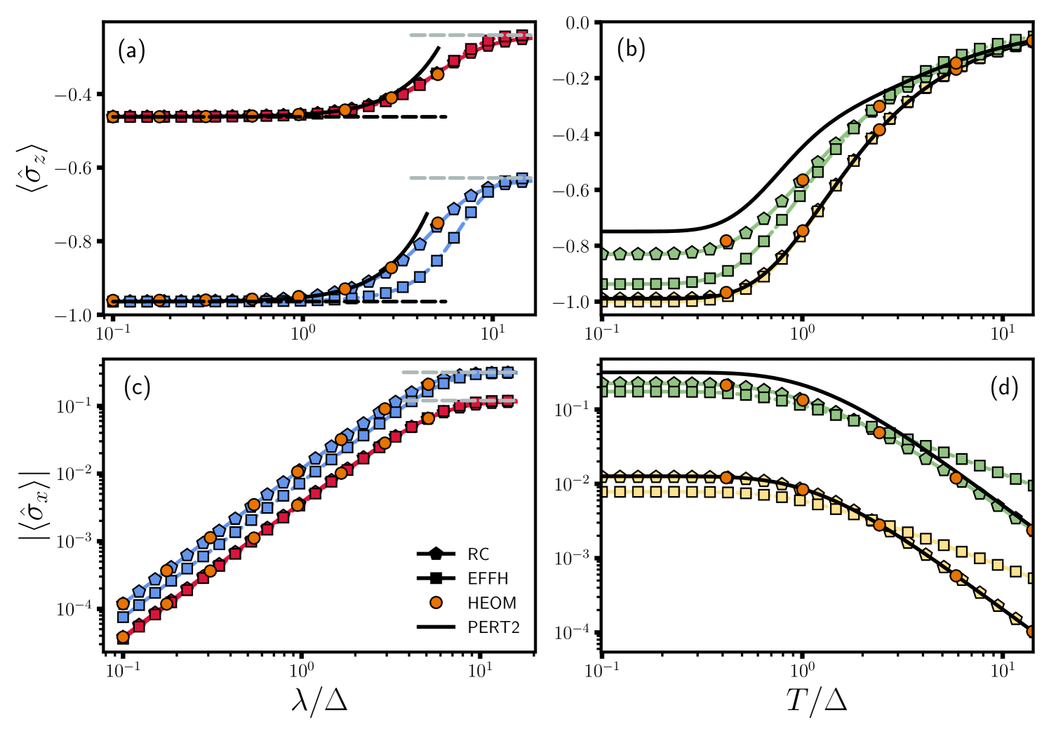
Figure 1: Comparison of the equilibrium state (top) polarization and the (bottom) coherence of the spin-boson model for $\theta=\pi/4$ as a function of the [(a),(c)] coupling strength $\lambda$ and [(b),(d)] temperature $T$. The calculations are shown for $\Omega=8\Delta$. Pentagons denote the quantities obtained from the RC approach using $M=50$, which is sufficient to guarantee convergence in the regime showed. Squares denote the result with the effective Hamiltonian model. Circles are computed from the hierarchical equations of motion ($N_{k}=15$ and $N_{c}=5$). In panels [(a),(c)], calculations are shown for two different values of the temperature. $T=0.5\Delta$ (blue) and $2.0\Delta$ (red). In panels [(b),(d)] two values of $\lambda=\Delta$ (yellow) and $5\Delta$ (green) are chosen. The dashed lines show the values in both the weak-coupling (black-dashed) and ultrastrong coupling (grey-dashed) approximations. The solid-black lines depict results using the second order correction to the Gibbs state. We use a Brownian spectral function with width parameter $\gamma=0.0075$.

II.3 Benchmarking the EFFH against numerically exact results

To test the accuracy of the EFFH method, we proceed to benchmark the expectation values of observables using the generalized spin-boson model [Eq. (9)] against some other approaches including numerically-exact simulations.

As for the EFFH method described before, we now recount its steps on the spin-boson model. First, the reaction coordinate mapping leads to

$$\hat{H}_{\rm RC} =\hat{H}_{S}+\Omega\left(\hat{a}^{\dagger}+\frac{\lambda}{\Omega}\hat{S}\right)\left(\hat{a}+\frac{\lambda}{\Omega}\hat{S}\right)$$ (10)

$$+\sum_{k}\omega_{k}\left(\hat{b}_{k}^{\dagger}+\frac{f_{k}}{\omega_{k}}(\hat{a}^{\dagger}+\hat{a})\right)\left(\hat{b}_{k}+\frac{f_{k}}{\omega_{k}}(\hat{a}^{\dagger}+\hat{a})\right),$$

where $\hat{a}$ and $\hat{a}^{\dagger}$ are canonical bosonic operators for the reaction coordinate PRXRC . It is clear from Eq. (8) that $\lambda$ grows as the system-bath coupling is increased. Henceforth, we thus regard $\lambda$ as the system-bath interaction energy. The residual bath operators can be related to the operators previous to the mapping, as described in Ref. Nazir18

Second, we apply the polaron transformation $\hat{U}_{P}={\rm{exp}}[\frac{\lambda}{\Omega}(\hat{a}^{\dagger}-\hat{a})\hat{S}]$ after the reaction coordinate mapping [step (ii) in Sec. II.2]. This operation transforms Eq. (10) to

$$\hat{\tilde{H}}_{\rm RC-P} =\hat{\tilde{H}}_{S}+\Omega\hat{a}^{\dagger}\hat{a}$$

$$+\sum_{k}\omega_{k}\left\{\left[\hat{b}_{k}^{\dagger}+\frac{f_{k}}{\omega_{k}}\Big{(}\hat{a}^{\dagger}+\hat{a}-\frac{2\lambda}{\Omega}\hat{S}\Big{)}\right]\right.$$

$$\times\left.\left[\hat{b}_{k}+\frac{f_{k}}{\omega_{k}}\Big{(}\hat{a}^{\dagger}+\hat{a}-\frac{2\lambda}{\Omega}\hat{S}\Big{)}\right]\right\}.$$ (11)

After the truncation of the degree of freedom of the reaction-coordinate [step (iii) in Sec. II.2], we find

$$\hat{H}^{\rm{eff}}=\hat{{H}}^{\rm{eff}}_{S}+\sum_{k}\omega_{k}\left[\hat{b}_{k}^{\dagger}-\frac{2\lambda f_{k}}{\Omega\omega_{k}}\hat{S}\right]\left[\hat{b}_{k}-\frac{2\lambda f_{k}}{\Omega\omega_{k}}\hat{S}\right].$$ (12)

Here,

$$\hat{{H}}^{\rm{eff}}_{S} =\hat{Q}_{0}\hat{U}_{P}\hat{H}_{S}\hat{U}_{P}^{\dagger}\hat{Q}_{0},$$ (13)

where $Q_{0}\mathrel{\vbox{\hbox{\scriptsize.}\hbox{\scriptsize.}}}=\ket{0}\bra{0}$ is the projector onto the ground-state subspace of the polaron-transformed reaction coordinate. We note that these operations leave the form in Eq. (9) unchanged. As described in Ref. PRXRC , the redefined system in Eq. (12) may be weakly coupled to the bath depending on the form of the original spectral function. For example, the Brownian function in Eq. (4) needs to be narrow to justify weak coupling at the end of the process ($\gamma\ll 1$ for the spin-boson model).

A simple calculation on the spin-boson model allows us to build the effective Hamiltonian of the system. Considering Eq. (9), we obtain

$$\hat{{H}}^{\rm{eff}}_{S} =\frac{\Delta}{2}\left[(1+e^{-\frac{2\lambda^{2}}{\Omega^{2}}})+(1-e^{-\frac{2\lambda^{2}}{\Omega^{2}}})\cos(2\theta)\right]\hat{\sigma}_{z}$$

$$+\frac{\Delta}{2}\left(1-e^{-\frac{2\lambda^{2}}{\Omega^{2}}}\right)\sin(2\theta)\hat{\sigma}_{x},$$ (14)

which is our EFFH for the spin-boson model. Since we work in the regime where the newly-mapped system Hamiltonian is weakly-coupled to the residual reservoir, we conjecture that the MFGS follows from the Gibbs state of the above Hamiltonian,

$$\hat{\rho}_{S}=\frac{e^{-\beta\hat{{H}}^{\rm{eff}}_{S}}}{{\rm Tr}_{S}\left(e^{-\beta\hat{{H}}^{\rm{eff}}_{S}}\right)}.$$ (15)

Note that calculating this state is straightforward since the dimensionality of the effective system Hamiltonian is simply a two-level system. In fact, the MFGS of the EFFH method can be obtained analytically as we showed in Ref. PRXRC .

To benchmark the ability of the EFFH method to describe the MFGS, we compute expectation values $\langle\hat{O}\rangle=\mathrm{Tr}[\hat{\rho}_{S}\hat{O}]$. For the spin-boson model, both $\hat{O}=\hat{\sigma}_{x}$ and $\hat{O}=\hat{\sigma}_{z}$ completely determine the state. As for the spectral function of the bath, we work with the Brownian spectral function [Eq. (4)] since it can be effectively simulated with alternative numerical techniques that will serve as benchmarks.

In Fig. 1 we display both $\langle\hat{\sigma}_{z}\rangle$ and $\langle\hat{\sigma}_{x}\rangle$ as a function of the coupling $\lambda$ at fixed temperature $T$ [Fig. 1(a),(c)] and as a function of $T$ at fixed $\lambda$ [Fig. 1(b),(d)]. We compare the equilibrium state obtained from the effective Hamiltonian treatment with results from the HEOM method, a numerically-exact approach. Appendix A provides technical details on the HEOM simulations. We further display simulations from the reaction-coordinate (RC) technique NickRC ; NickRC2 . This amounts to constructing the Gibbs state from the original system Hamiltonian $\hat{H}_{S}$ together with the degrees of freedom of the reaction coordinate [first line in Eq. (10)], followed by a partial trace over the degrees of freedom of the reaction coordinate. We remark that, for our chosen parameters, converging the HEOM equations becomes increasingly difficult as $\lambda$ increases, particularly in the low temperature regime. Nevertheless, it can be observed that for the results shown in Fig. 1 the reaction coordinate perfectly agrees with HEOM simulations. On the other hand, the EFFH approximation coincides with these results depending on both $\lambda$ and $T$. We also show in Fig. 1 results based on the 2^nd order perturbation scheme for the MFGS as presented in Ref. JanetPRL ; details of this calculation are provided in Appendix B. As expected, this approximation is only valid for moderate coupling strength $\lambda$. Limiting cases are also marked in Fig. 1 with dashed lines for the ultraweak coupling limit and ultrastrong coupling limits. Focusing our attention on the coupling-strength dependence of both polarization and coherences, we make the following observations based on Fig. 1:

(i) RC simulations perfectly agree with numerically exact results. We further verified this correspondence for a smaller characteristic frequency of the bath, $\Omega=1$ (not shown). Below, this excellent agreement allows us to test the EFFH method against RC simulations, rather than perform the computationally-costly HEOM calculations.

(ii) The EFFH treatment provides accurate results at both the ultraweak and ultrastrong coupling limits. Furthermore, it is correct quantitatively at all coupling regimes as long as the temperature is comparable to the spin splitting $\Delta$. The EFFH method struggles in the intermediate coupling regime either when the temperature is very low $T\ll\Delta$ or high $T\gtrsim\Omega$. In the former case, one requires the residual coupling to the bath to be sufficiently weak for the effective Hamiltonian treatment to provide accurate results for the MFGS. We can argue that at low $T$, correlations between the system and the reservoir are more prominent. This requires a more detailed description than our effective Hamiltonian for the physical effects to be captured. As for high temperatures, the extreme truncation of the RC limits the applicability of the EFFH method to the regime of $\Omega\gg T$. Looking at $\langle\hat{\sigma}_{x}\rangle$ in Fig. 1[(c),(d)], we particularly note that the coherence as calculated from the EFFH method are underestimated at low temperature and overestimated at high $T$.

(iii) The second-order correction to the Gibbs state only provides an accurate representation of the equilibrium state at weak-to-moderate coupling $\lambda$, while our effective Hamiltonian model is able to capture the full range of coupling. It is intriguing that the effective Hamiltonian model describes the ultrastrong coupling limit so well; this result was discussed in Ref. PRXRC .

Summarizing our benchmark efforts, we conclude that the EFFH method is a highly-reliable tool in situations when the residual coupling of the system to the bath is weak. It provides quantitatively-correct results to the MFGS at any coupling for temperatures in the range $\Delta\approx T\ll\Omega$. Significantly, with its minimal computational effort, the EFFH approach produces results on par with numerically-exact simulations.

III The Variational EFFH (var-EFFH) method

III.1 Presentation of Method

Due to the truncation of the polaron-transformed reaction coordinate harmonic ladder to the ground state, the EFFH method is limited to handle situations in which $\Omega\gg T,\Delta$. In physical terms, the collective bath’s degree of freedom to which the system is strongly coupled needs to be of high frequency relative to other energy scales in the system.

In this Section, we introduce a variational EFFH (var-EFFH) method, extending the original EFFH framework of Ref. PRXRC to handle the regime in which $\Omega\approx T,\Delta$. The outcome of the var-EFFH method is an effective Hamiltonian that depends on both the system-bath energy parameters and the bath’s temperature. Simulations presented in Sec. VI demonstrate that this tool indeed can capture the behavior of polarization of the spin-boson model when $\Omega$ is comparable to $\Delta$.

We recall the three steps in deriving the effective Hamiltonian, as summarized in Sec. II.2. The first step in the protocol involves performing a reaction coordinate transformation. In the second step, a polaron transformation is applied on the RC. In the variational EFFF approach, rather than applying a “normal” (or complete) polaron transform, we apply it in a variational manner defining

$$\hat{\tilde{H}}=\hat{U}_{P}\hat{H}_{\rm{RC}}\hat{U}^{\dagger}_{P},$$ (16)

with $\hat{U}_{P}={\rm{exp}}[\eta(\hat{a}^{\dagger}-\hat{a})\hat{S}]$. Here, $\eta$ is a real-valued variational parameter to be optimized later through the minimization of the free energy, based on the effective Gibbs state being thermal Cao2 , leading to $\eta\leq\lambda/\Omega$. The $\hat{U}_{P}$ transformation shifts the RC operator according to $\hat{a}\to\hat{a}-\eta\hat{S}$. The total Hamiltonian is given by

$$\hat{\tilde{H}}_{\rm RC-P} = \hat{\tilde{H}}_{S}+\Omega\left[\hat{a}^{\dagger}+\left(\frac{\lambda}{\Omega}-\eta\right)\hat{S}\right]\left[\hat{a}+\left(\frac{\lambda}{\Omega}-\eta\right)\hat{S}\right]$$ (17)

$$+ \sum_{k}\omega_{k}\left\{\left[\hat{b}^{\dagger}+\frac{f_{k}}{\omega_{k}}\Big{(}\hat{a}^{\dagger}+\hat{a}-2\eta\hat{S}\Big{)}\right]\right.$$

$$\times \left.\left[\hat{b}+\frac{f_{k}}{\omega_{k}}\Big{(}\hat{a}^{\dagger}+\hat{a}-2\eta\hat{S}\Big{)}\right]\right\}.$$

This Hamiltonian replaces Eq. (11). As we show below, $\eta$ is in general a function of the parameters of the system and its environment, including the temperature.

The third step in the procedure is to project this Hamiltonian onto a subspace in which the RC occupies only its ground state, $\ket{0}$. This is achieved using the operator $\hat{Q}_{0}=\ket{0}\bra{0}$. The result is the variational-effective Hamiltonian, and we highlight its dependence on $\eta$,

$$\hat{H}^{\rm{Veff}}(\eta) = \hat{Q}_{0}\hat{\tilde{H}}_{S}\hat{Q}_{0}+\Omega\left(\frac{\lambda}{\Omega}-\eta\right)^{2}\hat{S}^{2}$$ (18)

$$+ \sum_{k}\omega_{k}\left[\hat{b}^{\dagger}-\frac{2\eta f_{k}}{\omega_{k}}\hat{S}\right]\left[\hat{b}-\frac{2\eta f_{k}}{\omega_{k}}\hat{S}\right].$$

We now identify the system’s contribution to the var-EFFH, given by

$$\hat{H}^{{\rm Veff}}_{S}(\eta)=\hat{Q}_{0}\hat{\tilde{H}}_{S}\hat{Q}_{0}+\Omega\left(\frac{\lambda}{\Omega}-\eta\right)^{2}\hat{S}^{2}.$$ (19)

As expected, when performing the full polaron transform using $\eta=\frac{\lambda}{\Omega}$, the second term disappears and we recover Eq. (13). The bath Hamiltonian is simply $\hat{H}_{B}=\sum_{k}\omega_{k}\hat{b}^{\dagger}_{k}\hat{b}_{k}$, and the system-bath coupling is given by $\hat{H}_{I}=-2\eta\hat{S}\sum_{k}\frac{f_{k}}{\omega_{k}}\left(\hat{b}^{\dagger}+\hat{b}\right)$.

To find the parameter $\eta$, we minimize the Gibbs-Bogoliubov-Feynman upper bound on the free energy Silbey ; Cao2 given by the following expression

$$A_{B}=-\frac{1}{\beta}\ln\mathrm{Tr}\left[e^{-\beta[\hat{H}^{\text{Veff}}_{S}(\eta)+\hat{H}^{\text{Veff}}_{B}]}\right]+\langle\hat{H}^{\text{Veff}}_{I}\rangle_{\hat{H}^{\text{Veff}}_{S}(\eta)+\hat{H}^{\text{Veff}}_{B}}.$$ (20)

Here, the average is done over a canonical state with respect to the written Hamiltonian. Since $\langle\hat{H}^{\text{Veff}}_{I}\rangle_{\hat{H}^{\text{Veff}}_{S}(\eta)+\hat{H}^{\text{Veff}}_{B}}=0$ by construction, and the bath Hamiltonian is independent of the parameter $\eta$, we simply solve for $\eta$ using

$$\frac{\partial}{\partial\eta}\left[-\frac{1}{\beta}\ln\mathrm{Tr}_{S}\left(e^{-\beta\hat{H}^{\text{Veff}}_{S}(\eta)}\right)\right]=0.$$ (21)

This equation readily simplifies to

$$\mathrm{Tr}_{S}\left[e^{-\beta\hat{H}_{S}^{{\rm Veff}}(\eta)}\frac{d}{d\eta}\hat{H}_{S}^{{\rm Veff}}(\eta)\right]=0.$$ (22)

To compute the left hand side, one can build a closed-form expression for $\hat{H}_{S}^{{\rm Veff}}(\eta)$ for the particular model and set up a transcendental equation for $\eta$, which is then solved numerically. This approach is feasible if $\hat{S}^{2}\propto\hat{I}$ since computing the exponential term analytically can be a difficult task. An alternative approach is to solve the problem fully numerically by calculating the derivative of $\hat{H}_{S}^{{\rm Veff}}(\eta)$ with respect to $\eta$ then implementing the routine numerically. Once the optimal value of $\eta$ (denoted as $\eta_{v}$) has been obtained, the thermal state of the system is approximated as

$$\hat{\rho}^{\rm Veff}_{S}=\frac{e^{-\beta\hat{H}_{S}^{{\rm Veff}}(\eta_{v})}}{\mathrm{Tr}_{S}\left[e^{-\beta\hat{H}_{S}^{{\rm Veff}}(\eta_{v})}\right]},$$ (23)

where we emphasize again, $\eta_{v}=\eta(\lambda,\Omega,T,...)$.

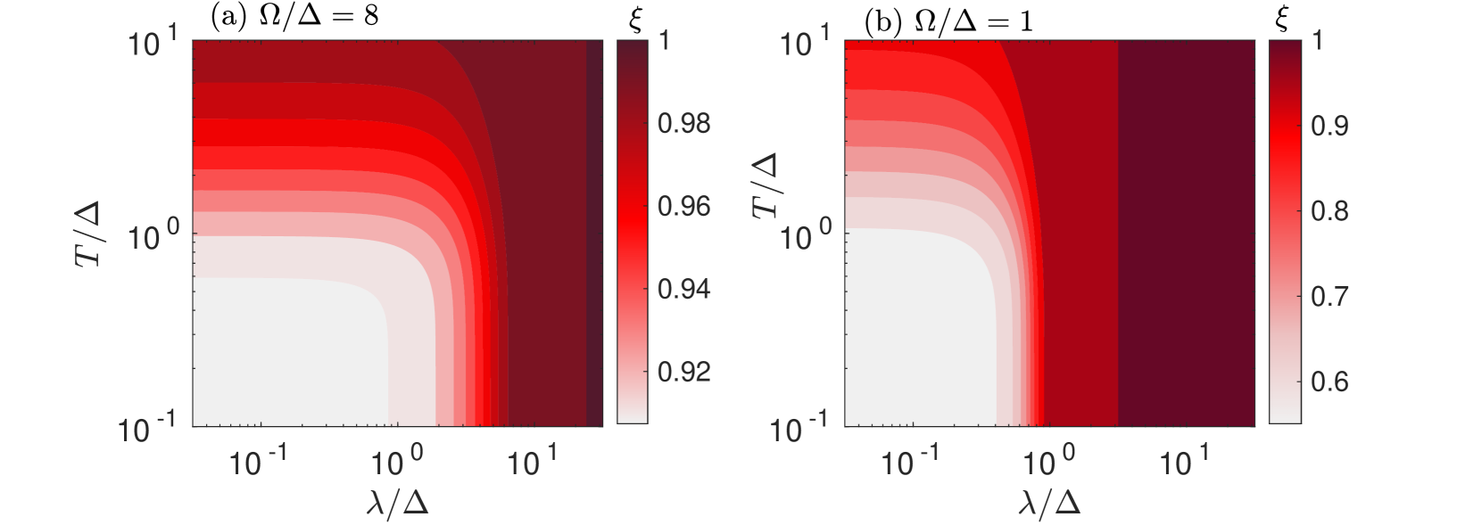
Figure 2: The variational parameter $\xi$ for the generalized spin-boson model as a function of coupling strength $\lambda$ and temperature $T$. This parameter, defined from the relation, $\eta_{v}=\xi\frac{\lambda}{\Omega}$, satisfies $0\leq\xi\leq 1$. When $\xi\to 1$, the variational treatment is redundant and the original EFFH method can be used. (a) $\Omega/\Delta=8$, (b) $\Omega/\Delta=1$. Other parameters are $\Delta=1$ and $\theta=\pi/4$.

III.2 Application to the generalized spin-boson model

Following the var-EFFH procedure described in Sec. III.1, we write down the corresponding var-EFFH system Hamiltonian for the spin-boson model,

$$\hat{H}^{\rm{Veff}}_{S}(\eta) = \frac{\Delta}{2}\left[(1+e^{-2\eta^{2}})+(1-e^{-2\eta^{2}})\cos(2\theta)\right]\hat{\sigma}_{z}$$

$$+ \frac{\Delta}{2}\left(1-e^{-2\eta^{2}}\right)\sin(2\theta)\hat{\sigma}_{x}+\Omega\left(\frac{\lambda}{\Omega}-\eta\right)^{2}.$$

To find the optimal value of $\eta$ we first compute

$$\frac{d}{d\eta}\hat{H}^{\rm{{\rm Veff}}}_{S}(\eta) = -2\Omega\left(\frac{\lambda}{\Omega}-\eta\right)$$

$$+ 2\Delta\eta e^{-2\eta^{2}}\left[(\cos(2\theta)-1)\hat{\sigma}_{z}+\sin(2\theta)\hat{\sigma}_{x}\right].$$

Then, using properties of Pauli matrices we analytically solve this problem from Eq. (22), revealing a transcendental equation of the form,

$$\frac{\lambda}{\Omega}=\eta_{v}\left[1+\frac{2\Delta e^{-4\eta_{v}^{2}}(1-\cos 2\theta)}{\Omega|\vec{v}|}\tanh\left(\frac{\beta\Delta}{2}|\vec{v}|\right)\right].$$

(26)

In the above expression, $|\vec{v}|$ depends on $\theta$ and $\eta_{v}$ as

$$|\vec{v}|=\sqrt{2(1+e^{-4\eta_{v}^{2}})+2(1-e^{-4\eta_{v}^{2}})\cos 2\theta}.$$ (27)

Setting $\eta_{v}\equiv\xi\frac{\lambda}{\Omega}$, which implies that $0\leq\xi\leq 1$, Eq. (26) transforms into

$$1=\xi\left[1+\frac{2\Delta e^{-4\xi^{2}\frac{\lambda^{2}}{\Omega^{2}}}(1-\cos 2\theta)}{\Omega|\vec{v}|}\tanh\left(\frac{\beta\Delta}{2}|\vec{v}|\right)\right].$$

(28)

It is clear that the effective parameter $\eta_{v}$ depends not only on the system-bath characteristic interaction energy scale $\lambda$ and frequency $\Omega$, but also on the bath temperature, extending the results of Ref. PRXRC . We now study particular cases and show how the variational parameter $\eta_{v}$ behaves in interesting limits.

(i) Ultrastrong coupling limit, $\lambda\xrightarrow{}\infty$. In this case, we get from Eq. (28) that

$$\xi=1,$$ (29)

which implies that the variational approach is redundant in the ultrastrong coupling limit. This is to be expected since we know that the EFFH method of Ref. PRXRC is exact for the spin-boson model in the ultrastrong coupling limit, as observed in Sec. II.3.

(ii) Asymptotically weak coupling $\lambda\xrightarrow{}0$. In this regime,

$$\xi \approx \frac{1}{1+\frac{\Delta}{\Omega}[1-\cos 2\theta]\tanh(\Delta\beta)}$$ (30)

$$\approx 1-\frac{\Delta}{\Omega}[1-\cos 2\theta]\tanh(\Delta\beta),$$

derived once requiring that $\Omega$ is the largest energy scale in the problem. Note that the correction to unity is small as a function of temperature since $\tanh\beta\Delta$ extends from $\beta\Delta$ at high temperature to one at very low temperatures.

(iii) Low temperature, $\beta\xrightarrow{}\infty$. In this case we find from Eq. (28) that

$$1=\xi\left[1+\frac{2\Delta e^{-4\xi^{2}\frac{\lambda^{2}}{\Omega^{2}}}(1-\cos 2\theta)}{\Omega|\vec{v}|}\right].$$ (31)

In this regime, the temperature only minimally impacts the variational parameter.

(iv) High temperature $\beta\xrightarrow{}\infty$. In this limit we find that

$$1=\xi\left[1+\beta\frac{\Delta^{2}e^{-4\xi^{2}\frac{\lambda^{2}}{\Omega^{2}}}(1-\cos 2\theta)}{\Omega}+\mathcal{O}(\beta^{3})\right].$$ (32)

In Fig. 2 we present simulations of $\xi$ as a function of system bath-coupling strength and temperature for $\theta=\pi/4$. We find that for $\Omega\gg T,\Delta$, the variational parameter $\xi$ does not reduce below 0.88 throughout the full range of coupling energies and temperatures. Thus, the expected correction due to the variational treatment is not large in this regime and the regular-nonvariational EFFH method is sufficient. On the other hand, for small values of the bath’s spectral frequency, $\Omega/\Delta=1$, corrections can be as substantial as 0.5.

We note that the variational approach corrects the EFFH method in the low temperature and weak-to-intermediate coupling regime. In the strong coupling limit and at high temperatures, we find that $\xi\approx 1$, thus one need not be concerned with these corrections.

The modification to the spin-boson Hamiltonian appears with the renormalization factor that we now define as

$$\kappa_{\rm E}\equiv e^{-2\xi^{2}\frac{\lambda^{2}}{\Omega^{2}}}.$$ (33)

Using $\xi=1$, this expression reduces to the non-variational treatment of Ref. PRXRC .

IV Comparative analysis: The variational polaron MFGS

The polaron transform is a well-established and popular treatment to study strong system-bath coupling effects in spin-boson type models. In particular, it has been extensively employed to study heat transfer in nonequilibrium settings where a few level system(s) are coupled to two or more reservoirs diodeSC0 ; diodeSC1 ; diodeSC2 ; diodeSC1b ; Pollock_2013 ; Hsieh_2019 ; Zhang_2015 ; Zhang_2015_2 ; Liu_2018 ; Wang_2015 ; Liu_2017 ; Koch_2011 ; Dominguez_2011 ; Lu_2019 ; Wachtler_2020 ; Koch_2010 ; Chen_2019 ; Wang_2017 . Furthermore, the polaron transform has also been utilized to analytically and numerically gain insights on experimental works on superconducting circuits Dai_2022 ; Agarwal_2013 ; Shi_2018 . Non-Markovian dynamics in cavity quantum electrodynamics have been also examined using polaron transformed QME Zhangg_2022 ; bn_2021 . Critical phenomena in dissipative models Kopylov_2019 and the robustness of topological order in two-dimensional spin lattice coupled to bosonic reservoir Pedrocchi_2013 are other recent examples where the transform was found useful. In the context of quantum thermodynamics JanetRev ; Cao1 ; Cao2 ; Cao3 , although the polaron transform was used to build the MFGS in the intermediate system-bath coupling regime, the discussion has been mostly limited to the spin-boson model.

In what follows, we first introduce the procedure of obtaining an approximate MFGS for a general open system using the variational polaron transformation. We then exercise this method on the generalized spin-boson model described in Eq. (9). We discuss the relationship of the MFGS as obtained from the variational polaron (var-POL) to the MFGS of the var-EFFH method. Finally, we present simulations for the spin polarization and coherences for baths with spectral function peaked either at high or low frequencies.

IV.1 Polaronic MFGS: Generic open quantum system

The variational polaron MFGS was constructed for the spin-boson model and benchmarked against other methods Cao1 ; Cao2 . Here, we present the generalization of the procedure to obtain the MFGS for a generic open quantum system as in Eq. (1). The polaron transform is generated here by the following unitary,

$$\hat{W}=\exp(-\mathrm{i}\hat{S}\hat{B}/2),$$ (34)

where $\hat{B}=2\mathrm{i}\sum_{k}\frac{f_{k}}{\nu_{k}}(\hat{c}^{\dagger}_{k}-\hat{c}_{k})$ and $\hat{S}$ is the system operator coupled to the bath, introduced in Eq. (1). The transformation is referred to as “full-polaron” if the variational parameters $\{f_{k}\}$ are simply set to $\{t_{k}\}$, the original system-reservoir couplings. If, instead, the optimal values for $\{f_{k}\}$ are obtained by minimizing the Gibbs-Bogoliubov-Feynman upper bound on the free energy, the transform is called “variational” Silbey ; Silbey_2 . Performing the transform on the Hamiltonian Eq. (1) we obtain

$$\hat{H}^{\text{pol}}= \hat{W}\hat{H}_{S}\hat{W}^{\dagger}+\hat{S}^{2}\sum_{k}\frac{(t_{k}-f_{k})^{2}}{\nu_{k}}+\hat{H}_{B}$$ (35)

$$+ \hat{S}\sum_{k}(t_{k}-f_{k})\left(\hat{c}^{\dagger}_{k}+\hat{c}_{k}\right),$$

with $\hat{H}_{B}=\sum_{k}\nu_{k}c^{\dagger}_{k}c_{k}$.

The next stage in building a Hamiltonian of mean force is to add and subtract the bath-averaged expectation value of the transformed system Hamiltonian. This ensures that the thermal average of the interaction operator diminishes. We thus write down the above total Hamiltonian as

$$\hat{H}^{\text{pol}}=\hat{H}^{\text{pol}}_{S}+\hat{H}^{\text{pol}}_{B}+\hat{H}^{\text{pol}}_{I},$$ (36)

identifying the system, bath, and the interaction terms, respectively, by

$$\hat{H}^{\text{pol}}_{S} = \langle\hat{W}\hat{H}_{S}\hat{W}^{\dagger}\rangle_{\hat{H}_{B}}+\hat{S}^{2}\sum_{k}\frac{(t_{k}-f_{k})^{2}}{\nu_{k}},$$

$$\hat{H}^{\text{pol}}_{B} = \hat{H}_{B},$$

$$\hat{H}^{\text{pol}}_{I} = \hat{W}\hat{H}_{S}\hat{W}^{\dagger}-\langle\hat{W}\hat{H}_{S}\hat{W}^{\dagger}\rangle_{\hat{H}_{B}}$$ (37)

$$+ \hat{S}\sum_{k}(t_{k}-f_{k})\left(\hat{c}^{\dagger}_{k}+\hat{c}_{k}\right).$$

The system’s Hamiltonian $\hat{H}^{\rm pol}_{S}$ includes two terms. First, the original system Hamiltonian is rotated to the polaron frame. Second, a new term emerges, related to the original system-bath coupling operator. This second term in particular could realize bath-induced interactions between individual impurities (e.g., spins) immersed in a bath. We now make the assumption that the polaron-transformed Hamiltonian is weakly coupled to the bath, thus the MFGS can be approximated from the system Hamiltonian as

$$\hat{\rho}^{\rm pol}_{S}=\frac{e^{-\beta\hat{H}^{\rm pol}_{S}}}{\mathrm{Tr}\left(e^{-\beta\hat{H}^{\rm pol}_{S}}\right)}.$$ (38)

We note that it is often useful to diagonalize the system operator $\hat{S}$ that couples to the bath modes prior to the polaron transform. This is indeed the case in the general spin-boson model where $\hat{S}=\cos(\theta)\hat{\sigma}_{z}+\sin(\theta)\hat{\sigma}_{x}$. Rotating $\hat{S}$ to $\hat{\sigma}_{z}$ via the rotation matrix $\hat{R}=\exp(-\frac{\mathrm{i}}{2}\theta\hat{\sigma}_{y})$ allows us to compute the nested commutator involved in $\langle\hat{W}\hat{H}_{S}\hat{W}^{\dagger}\rangle_{\hat{H}_{B}}$ with more ease. Once the transformed Hamiltonian is written down, the optimal values for $\{f_{k}\}$ are obtained by minimizing the free energy given by an expression analogous to Eq. (20),

$$A_{B}=-\frac{1}{\beta}\ln\mathrm{Tr}\left[e^{-\beta(\hat{H}^{\rm pol}_{S}+\hat{H}^{\rm pol}_{B})}\right]+\langle\hat{H}^{\rm pol}_{I}\rangle_{\hat{H}^{\rm pol}_{S}+\hat{H}^{\rm pol}_{B}}.$$ (39)

Since $\langle\hat{H}^{\rm pol}_{I}\rangle_{\hat{H}^{\rm pol}_{S}+\hat{H}^{\rm pol}_{B}}=0$ by construction, and the bath Hamiltonian is independent of the parameters $\{f_{k}\}$, the minimization of the free energy requires solving

$$\frac{\partial}{\partial f_{k}}\left[-\frac{1}{\beta}\ln\mathrm{Tr}_{S}\left(e^{-\beta\hat{H}^{\rm pol}_{S}}\right)\right]=0.$$ (40)

Once the set of parameters $f_{k}$ is obtained, it is used in Eq. (37) to build the system’s Hamiltonian, and then proceed to compute the MFGS.

IV.2 Application to the spin-boson model

We apply the var-POL approach on the general spin-boson model and construct the approximate MFGS. Applying Eq. (37) on the model (9), we write down $\hat{H}^{\rm pol}=E_{0}\hat{I}+\hat{H}^{\rm pol}_{S}+\hat{H}^{\rm pol}_{B}+\hat{H}^{\rm pol}_{I}$ with

$$\hat{H}^{\rm pol}_{S} = \Delta\left[\cos^{2}(\theta)+\sin^{2}(\theta)\kappa_{P}\right]\hat{\sigma}_{z}$$ (41)

$$+ \Delta\cos(\theta)\sin(\theta)(1-\kappa_{P})\hat{\sigma}_{x},$$

$$\hat{H}^{\rm pol}_{B} = \sum_{k}\nu_{k}\hat{c}^{\dagger}_{k}\hat{c}_{k},$$ (42)

$$\hat{H}^{\rm pol}_{I} = \hat{V}_{x}\hat{\sigma}_{x}+\hat{V}_{y}\hat{\sigma}_{y}+\hat{V}_{z}\hat{\sigma}_{z}.$$ (43)

Here, $\hat{H}^{\rm pol}_{S}$ is obtained by first diagonalizing the system operator $\hat{S}$ via the rotation matrix $\hat{R}=\exp(-\frac{\mathrm{i}}{2}\theta\hat{\sigma}_{y})$. We then perform the var-POL transform with the new interaction term, being the $\hat{\sigma}_{z}$ operator. Once we construct the new system Hamiltonian, we rotate it back to the original basis via $\hat{R}^{\dagger}$. $E_{0}=\sum_{k}\frac{(f_{k}-t_{k})^{2}}{\nu_{k}}$ is a trivial energy shift. The system’s Hamiltonian depends on $0\leq\kappa_{P}\leq 1$, which is given by

$$\kappa_{P}=\exp\left[-2\sum_{k}\frac{f^{2}_{k}}{\nu^{2}_{k}}\coth\left(\frac{\beta\nu_{k}}{2}\right)\right].$$ (44)

To be concrete, at specific angles of interest the system’s Hamiltonian is given by

$$\hat{H}^{\rm pol}_{S}(\theta=0) =\Delta\hat{\sigma}_{z},$$ (45)

$$\hat{H}^{\rm pol}_{S}(\theta=\pi/2) =\Delta\kappa_{P}\hat{\sigma}_{z},$$ (46)

$$\hat{H}^{\rm pol}_{S}(\theta=\pi/4) =\frac{\Delta}{2}\left[\left(1+\kappa_{P}\right)\hat{\sigma}_{z}+\left(1-\kappa_{P}\right)\hat{\sigma}_{x}\right].$$ (47)

The angle $\theta=0$ corresponds to the exactly-solvable pure decoherence model. For $\theta=\pi/2$, we retrieve the standard spin-boson model with renormalized spin splitting $\Delta\kappa_{P}$. In between, for $\theta=\pi/4$, the polaron-transformed system’s Hamiltonian includes both spin splitting and tunneling between levels.

It can be readily shown that Eq. (41) has the exact same form as the EFFH for the same system, as shown in Eq. (LABEL:eq:HSBVeff). The two approaches thus build a similar approximation for the MFGS with $\kappa_{P}$ of the var-POL mirroring the $\kappa_{E}$ factor appearing in the var-EFFH Hamiltonian, Eq. (33). However, calculating $\kappa_{P}$ is significantly more complicated numerically than evaluating $\kappa_{E}$, since the optimization process in the former involves many (in principle infinite) modes, leading at times to convergence problems at strong coupling, as we show below in simulations.

As for the system-bath coupling operators, the bath’s operators coupled to the system are notably more complicated in the polaron approach than those showing up in Eq. (LABEL:eq:HSBVeff). In the polaron-transformed spin-boson model we obtain

$$\hat{V}_{x} = \sin(\theta)\sum_{k}(t_{k}-f_{k})(\hat{c}^{\dagger}_{k}+\hat{c}_{k})-\Delta\sin(\theta)\cos(\theta)\left[\cos(\hat{B})-\kappa_{P}\right],$$

$$\hat{V}_{y} = -\Delta\sin(\theta)\sin(\hat{B}),$$

$$\hat{V}_{z} = \cos(\theta)\sum_{k}(t_{k}-f_{k})(\hat{c}^{\dagger}_{k}+\hat{c}_{k})+\Delta\sin^{2}(\theta)\left[\cos(\hat{B})-\kappa_{P}\right].$$ (48)

These terms however do not impact the MFGS as constructed from Eq. (38). We recall that the parameters $\{f_{k}\}$ are obtained through a variational approach. As detailed in Appendix. C, we rewrite the relationship between the physical coupling energies $\{t_{k}\}$ and the sought-after parameters $\{f_{k}\}$ through a self-consistent set of equations

$$f_{k}=F(\nu_{k})t_{k},$$ (49)

where, for the selected models, we get

$$F(\nu_{k},\theta=\pi/2)=\left[1+\tanh\left(\beta\Delta\kappa_{P}\right)\coth\left(\frac{\beta\nu_{k}}{2}\right)\frac{2\Delta\kappa_{P}}{\nu_{k}}\right]^{-1},$$

$$F(\nu_{k},\theta=\pi/4)=\Bigg{[}1+\tanh\left(\beta\Delta\sqrt{\frac{1+\kappa_{P}^{2}}{2}}\right)\coth\left(\frac{\beta\nu_{k}}{2}\right)\sqrt{\frac{2}{1+\kappa_{P}^{2}}}\frac{\Delta\kappa_{P}^{2}}{\nu_{k}}\Bigg{]}^{-1}.$$ (50)

The parameter $\kappa_{P}$ is defined in Eq. (44). In practice, the numerical procedure to solve for the set of variational parameters $\{f_{k}\}$ involves first constructing a finite-truncated set of system-bath coupling energies $\{t_{k}\}$ based on the model spectral function and initializing $\kappa_{P}$ as a guess. Then, we calculate $\{f_{k}\}$ using Eqs. (49)-(50), regenerate the dressing parameter $\kappa_{P}$ in Eq. (44), and iterate this process until convergence.

At the technical level, the main differences between the two procedures, the var-EFFH mapping and the var-POL, are that in the former, we first extract a collective degree of freedom from the bath (reaction coordinate), then rotate it individually to the polaron frame. In contrast, in the var-POL framework a polaron transform is operated directly on the original Hamiltonian, affecting all modes in the bath. As for the resulting Hamiltonian, the distinction lies in the interaction terms: although the var-POL produces a system Hamiltonian analogous to that from the EFFH method, interaction terms are modified. This difference between the methods does not show up in the MFGS, but it will be displayed in the study of dynamics, e.g., via the usual weak-coupling master equation technique. Concretely, in case of the general spin-boson model, the var-POL transform will induce all $\hat{\sigma}_{x}$, $\hat{\sigma}_{y}$, and $\hat{\sigma}_{z}$ couplings with the bath displacement operators as described by Eq. (43) and Eq. (48). This is in contrast to the EFFH which retains its original coupling structure, see Eq. (18).

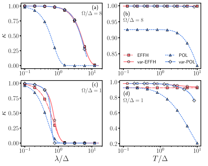
Figure 3: The renormalization factor $\kappa$ for the generalized spin-boson model computed via Eq. (44) for the polaron (blue triangles) and variational polaron (diamonds). For the effective approach (red squares) and the variational effective approach (circles) we employ Eq. (33). $\kappa$ is plotted as a function of (a)-(c) coupling strength $\lambda$ and (b)-(d) temperature $T$. Results are shown for $\Delta=1$, $\theta=\pi/4$, $T=\Delta$ (a)-(c), and $\lambda=0.2\Delta$ (b)-(d).

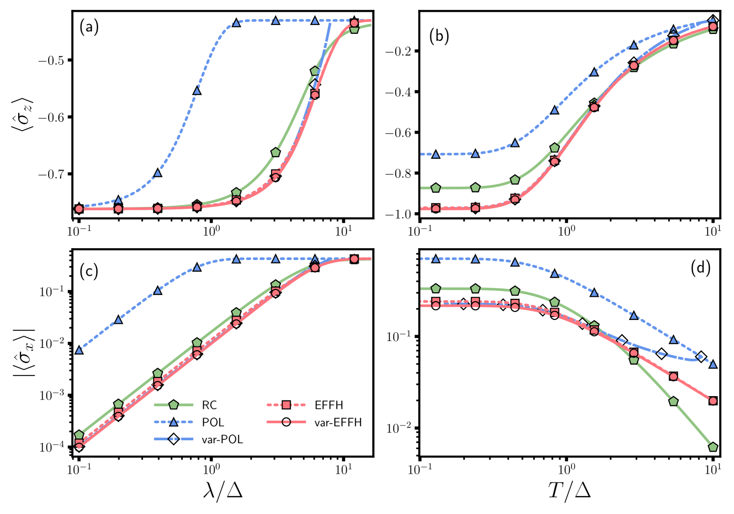
Figure 4: The $\langle\hat{\sigma}_{x}\rangle$ and $\langle\hat{\sigma}_{z}\rangle$ spin polarizations for the generalized spin-boson model as a function of (a) and (c) coupling strength $\lambda$ and (b) and (d) temperature $T$. Results are shown for the effective approach (red squares), variational effective approach (circles), polaron (blue triangles) and variational polaron (diamonds) and the reaction coordinate method (green pentagons). Parameters are: $\Delta=1$, $\theta=\pi/4$, $\Omega=8$, $T=1$ (a-c), and $\lambda=4$ (b-d).

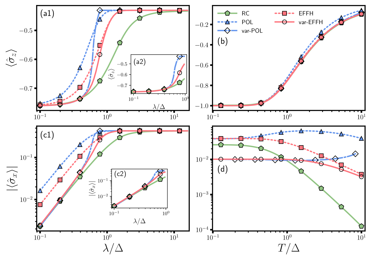
Figure 5: The $\langle\hat{\sigma}_{x}\rangle$ and $\langle\hat{\sigma}_{z}\rangle$ spin polarizations for the generalized spin-boson model as a function of (a) and (c) coupling strength $\lambda$ and (b) and (d) temperature $T$. Results are shown for the effective approach (red squares), variational effective approach (circles), polaron (blue triangles) and variational polaron (diamonds) and the reaction coordinate method (green pentagons). Parameters are: $\Delta=1$, $\theta=\pi/4$, $\Omega=1$, $T=1$ (a-c), and $\lambda=0.2$ (b-d). The small panels (a2) and (c2) zoom over the weak-coupling regime.

V MFGS: Analytical results

We found that for the generalized spin-boson model, the EFFH and the POL methods generate the same form for the Hamiltonian of the system, Eq. (LABEL:eq:HSBVeff) and Eq. (41), respectively. The only difference between them is the scheme for achieving the parameter $\kappa=\{\kappa_{E},\kappa_{P}\}$, and the resulting value. We recall that $\kappa$ embodies the impact of the system-bath coupling on the system through a renormalization effect to level splitting and the generation of new terms. Using the EFFH/POL form for the system’s Hamiltonian, we calculate the MFGS, arriving at PRXRC

$$\hat{\rho}_{S}=\frac{1}{2}\left[\hat{I}-\frac{(\vec{v}\cdot\vec{\sigma})}{|\vec{v}|}\tanh\left(\frac{\beta\Delta}{2}|\vec{v}|\right)\right],$$ (51)

where $\vec{\sigma}=(\hat{\sigma}_{x},\hat{\sigma}_{y},\hat{\sigma}_{z})$ and

$$\vec{v}=[(1-\kappa)\sin(2\theta),0,(1+\kappa)+(1-\kappa)\cos(2\theta)].$$

Here, $\hat{v}$ is the unit vector associated to $\vec{v}$ of magnitude

$$|\vec{v}|=\sqrt{2(1+\kappa^{2})+2(1-\kappa^{2})\cos(2\theta)}.$$ (53)

Using these expressions and choosing as an example the angle $\theta=\pi/4$, we get a closed-form expression for the polarization, covering its behavior at arbitrary coupling strength,

$$\langle\hat{\sigma}_{z}\rangle=-\frac{1}{|\vec{v}|}(1+\kappa)\tanh\left(\frac{\beta\Delta}{2}|\vec{v}|\right).$$ (54)

This result approaches the canonical solution in the ultraweak coupling limit, which corresponds to $\kappa=1$,

$$\langle\hat{\sigma}_{z}\rangle\xrightarrow{\kappa\to 1}-\tanh\left(\beta\Delta\right).$$ (55)

In contrast, in the ultrastrong coupling limit we get

$$\langle\hat{\sigma}_{z}\rangle\xrightarrow{\kappa\to 0}-\frac{1}{\sqrt{2}}\tanh\left(\frac{\beta\Delta\sqrt{2}}{2}\right),$$ (56)

which approaches (in magnitude) $1/\sqrt{2}$ at low temperatures and $\beta\Delta/2$ at high temperatures.

As for coherences, we find that (for the particular case of $\theta=\pi/4$)

$$\langle\hat{\sigma}_{x}\rangle=-\frac{1}{|\vec{v}|}(1-\kappa)\tanh\left(\frac{\beta\Delta}{2}|\vec{v}|\right).$$ (57)

While in the weak coupling limit the coherences vanish, in the ultrastrong limit we find that they sustain the same value as that of the polarization,

$$\langle\hat{\sigma}_{x}\rangle\xrightarrow{\kappa\to 0}-\frac{1}{\sqrt{2}}\tanh\left(\frac{\beta\Delta\sqrt{2}}{2}\right).$$ (58)

These expressions were derived for $\theta=\pi/4$; the behavior of the expectation values for any $\theta$ is straightforward to obtain PRXRC .

At the mathematical level, the expressions for the polarization and the coherence are identical between the POL and the EFFH methods, both variational and non-variational. However, at finite coupling we have that $0<\kappa<1$ and so the actual values of $\kappa_{E}$ and $\kappa_{P}$ differ, leading to quantitative deviations between the methods.

VI Simulations

We established in Fig. 1 the validity of the numerical reaction coordinate approach NickRC on the equilibrium spin-boson model by benchmarking it against numerically-exact simulations. In this Section, our focus is on the var-EFFH method, and we ask three questions: (i) How well does the var-EFFH method perform compared to RC simulations? We assume that the latter results are very close to numerically-exact simulations in our parameter range. (ii) What is the range of parameters where it is imperative to employ the var-EFFH tool, compared to the non-variational treatment? (iii) How do the var-EFFH and the var-POL methods compare in their ability to treat strong coupling effects?

We begin in Fig. 3 by comparing parameters in the effective models generated by the var-POL and the var-EFFH methods, as well as with their non-variational analogs. We present simulations of the renormalization parameters $\kappa_{P}$ and $\kappa_{E}$, defined respectively in Eq. (44) for the polaron method and in Eq. (33) for the EFFH treatment. In the spin-boson model, this parameter uniquely impacts the original Hamiltonian by system-bath coupling effects. The renormalization parameters are studied as a function of the coupling strength in Fig. 3(a) and Fig. 3(c) and as a function of temperature in Fig. 3(b) and Fig. 3(d), for the particular choice of $\theta=\pi/4$. We show both the “bare” parameters without a variational treatment and variational results. We test the behavior of $\kappa$ for both large $\Omega$ in Fig. 3(a)-(b) and small $\Omega$ Fig. 3(c)-(d).

Beginning with the $\lambda$ dependence, in Fig. 3(a), we report a nearly-perfect agreement between the EFFH and var-EFFH for $\Omega\gg T,\Delta$, suggesting that the variational scheme is not necessary in this regime, which is expected. Furthermore, the var-POL approach predicts very similar trends for the coupling dependence, from ultraweak well into the intermediate coupling regime. However in the ultrastrong coupling limit the var-POL algorithm did not converge. Lastly, the full polaron displays stark numerical deviations. This is to be expected since a full-polaron transform is suitable for Ohmic spectral functions Legget ; Weiss but not for (narrow) Brownian spectral functions. Repeating the analysis for small $\Omega$, of order of both the spin splitting energy and the temperature, we find that the var-EFFH brings a smaller renormalization ($\kappa\approx 1$) than the full EFFH, with more qualitative deviations of the var-POL method at strong coupling.

In Fig. 3(b) and Fig. 3(d) we display the temperature dependence of $\kappa$. We point out the lack of temperature dependence in the non-variational EFFH approach; the influence of the bath’s temperature does not come into the protocol of generating the effective Hamiltonian in Ref. PRXRC . In contrast, the var-EFFH method that we introduced in this work shows temperature dependence due to the inclusion of the temperature and other system parameters in the transcendental equation, Eq. (44). The dependence of $\kappa_{E}$ on temperature is more pronounced at high temperatures and less so at low temperatures, which is expected. At the chosen coupling strength, the dependence on temperature is modest. The var-POL approach also displays a temperature dependence: At low temperature, the induced renormalization effects are similar to those observed by the var-EFFH method. Deviations show up at higher temperatures ($T/\Delta>1$) and for small $\Omega$, where there is a rapid suppression in the var-POL renormalization parameter. Lastly, the full polaron transformation significantly overestimates the effect of dressing, especially at high temperatures.

To study the MFGS, we analyze physical observables of the spin, $\langle\hat{\sigma}_{z}\rangle$ and $\langle\hat{\sigma}_{x}\rangle$, displayed in Fig. 4 and Fig. 5 for high and low characteristic bath frequencies, respectively. We compare the following approaches: The non-variational EFFH and POL methods, along with their variational analogs. We further display RC simulations (green pentagons) serving as a benchmark to verify the numerical accuracy of each approach. In Fig. 4(a) and Fig. 4(c) we display the coupling-strength dependence of the spin polarization and coherences. We report a near-perfect agreement between the EFFH, var-EFFH and the var-POL methods, which are also qualitatively similar to the RC technique. On the other hand, the full polaron method falls short again, underestimating the spin polarization and overshooting the coherence. The temperature dependence of the spin is presented in Fig. 4(b) and Fig. 4(d). In Fig. 4(b) we see similar trends as before, namely, the spin polarization is well approximated by the EFFH, var-EFFH and the var-POL approach, with relatively small deviations from the RC method; the full polaron approach shows once again larger discrepancies. As for the coherences shown in Fig. 4(d), they are not well captured in the high temperature limit by any of the approximate approaches: The scaling of the coherences with temperature at high temperature, predicted by the var-EFFH method is different from that of the RC technique. This deviation can be rationalized by recalling that the EFFH method is not suitable to high temperature settings given the truncation of the reaction coordinate to its ground state.

Next, in Fig. 5 we study analogous results compared to Fig. 4, yet for small bath frequency, with $\Omega$ being comparable to both $\Delta$ and $T$. The EFFH method is not expected to perform well in this parameter range given that it is based on a complete truncation of the reaction coordinate. This truncation is justified when there is a separation of energy scales of the bath from the system with high levels of the reaction coordinate (above thermal energy) approximately not populated. Focusing first on the behavior of polarization and coherences as a function of coupling strengths in Fig. 5(a) and Fig. 5(c), we note on the substantial success of the var-EFFH to capture the weak-to-intermediate coupling regime. The var-POL method is also successful in this regime, but at a certain value of the coupling it “collapses” into the inaccurate non-variational polaron result. As for the temperature dependence shown in Fig. 5, we focus on the weak coupling limit where the methods perform relatively well. We note that the polarization in Fig. 5(b) is very well captured by all the approaches employed. However, coherences in Fig. 5(d) are captured only qualitatively by the variational and non-variational EFFH methods. Nevertheless, this moderate success should be contrasted with the fact that the POL and the var-POL methods are unreliable in the small $\Omega$ case beyond low temperatures, providing incorrect (non-monotonic) trends.

Returning to questions posed at the beginning of this Section, our results point towards the following conclusions: (i) The var-EFFH method can be used with confidence across the entire system-bath coupling range as long as $\Omega>T,\Delta$. Furthermore, it can be employed at smaller values of $\Omega$ provided one is interested only in the regime of weak-to-intermediate coupling energy. (ii) The non-variational EFFH method is powerful and qualitatively correct whenever $\Omega\gg T$. Given its analytical form and simplicity, we argue in favor of this approach over the var-EFFH technique, since the latter requires a numerical optimization procedure to build its parameter. (iii) The non-variational polaron approach should be avoided if one is interested in the description of equilibrium states at strong coupling when using structured spectal functions. The var-POL technique in contrast performs well over a broad range of both coupling strength and temperature. Its main caveat lies in its “collapse” to full polaron results (or altogether non-convergence) in difficult parameter regimes, e.g., at ultrastrong couplings or at high temperatures, unlike the EFFH method that is always well behaved.

VII Discussion and Summary

We have focused on approximation schemes for the equilibrium state of a quantum system, the so-called MFGS. Our main focus has been the EFFH method that was first introduced in Ref. PRXRC , which is semi-analytical and handles strong system-bath coupling effects. Using the spin-boson model as a case study, we validated the EFFH method from weak to strong coupling, developed a variational flavor that extends the regime of applicability of the original method and compared it to the well-known polaron-transform treatment. In more details, our contributions are threefold:

(i) First, we examined the effectiveness of the EFFH method in building an approximate MFGS of the general spin-boson model by benchmarking it against the numerically-exact HEOM. In addition to the excellent quantitative agreement in the ultraweak and ultrastrong system-bath coupling limits, we observed a correct qualitative behavior at all intermediate couplings. Furthermore, we emphasize that for the specific temperatures in the range $\Delta\approx T\ll\Omega$ we find quantitatively-accurate results of the EFFH MFGS in all system-bath coupling strength.

(ii) The basic drawback of the EFFH treatment as introduced in Ref. PRXRC is that it is limited to parameter regimes where the typical energy scale of the system ($\Delta$) is close to the bath temperature ($T$) while sitting below the characteristic frequency of the bath ($\Omega$). To relax this limitation, we developed here the var-EFFH method where the original, full polaron transform, enacted after the RC mapping, is replaced with a variational one. The consequence of the variational polaron procedure is the dressing of the original system parameters with not only the residual coupling ($\lambda$) and the characteristic frequency of the bath ($\Omega$), but also with the bath temperature ($T$). As a result, we extended the applicability of the original EFFH method even to parameter regimes where $\Omega\simeq\Delta$. In particular, the var-EFFH method captures the MFGS in the weak-to-intermediate coupling regime especially well. However, although the var-EFFH method can be used even when $\Omega$ is not large relative to the system energy scale $\Delta$ and the bath temperature $T$, the chosen values for $\Delta$ and $T$ must still be on the same scale, particularly when studying coherences. High temperature effects cannot be well captured given the extreme truncation of the reaction coordinate, while low-temperature effects are still missing in the construction of the MFGS; possibly due to the development of strong system-bath correlations. These aspects require further investigation.

(iii) Equipped with the new var-EFFH technique, we compare its efficacy in describing the MFGS against the popular polaron transformation. Both the POL/var-POL approach lead to the same system Hamiltonian structure as the EFFH/var-EFFH framework, where the only distinction lies in the value of the renormalized system parameters captured by $\kappa_{P}$ and $\kappa_{E}$, respectively. Qualitatively analogous simulation results were obtained in predicting the MFGS using the two methods. However, for structured spectral functions, the EFFH is advantageous over the polaron technique in accuracy, computational cost and stability. While the methods display the same physics, the EFFH is simpler and more robust in computations.

We focused in this paper on the spin-boson model to understand and test the validity of the variational and non-variational EFFH and POL approaches. For the spin-boson model, we showed that these approaches built an identical system Hamiltonian, only with different parameters. In Appendix D and Appendix E, we further examine the Caldeira-Leggett model of a single harmonic mode bilinearly coupled to harmonic bath, and derive the system’s Hamiltonian under the EFFH and the POL methods. We find that the two methods again reach the same result: The system’s Hamiltonian after the EFFH mapping is identical to the original one only with a constant shift, thus indicating that the state of the system is still the standard Gibbs state, even at strong coupling. This conclusion indeed holds at high temperatures, $\Delta\ll T$, as discussed in Refs. Lutz:2011Eq ; HO1 ; HO2 ; HO3 ; HO4 .

A natural extension of our work is to test the validity of the var-EFFH treatment in obtaining the MFGS for a variety of bath spectral functions. In our work, we only studied Brownian-structured spectral functions where the RC is most-easily computed. To capture other situations, e.g., a structured bath with multiple peaks or the popular Ohmic-type spectral functions, the procedure of the RC extraction has to be made into a numerical process. Once a reliable machinery of extracting RC modes from the bath is established, the EFFH method could be trivially executed.

Another avenue for the var-EFFH treatment is to study systems with multiple building blocks with or without direct interactions between them Archak ; Kawai_2019 . In the case of noninteracting spins coupled to a common bath, bath-mediated spin-spin interaction terms arise beyond weak coupling. This was recently demonstrated numerically, using the RC method in Ref. Brenes_2023 , with applications to quantum thermometry. However, studying the development of cooperative effects with analytical tools such as the var-EFFH method is still missing.

The EFFH method can be readily used to treat systems out-of-equilibrium, as demonstrated in Ref. PRXRC . With it generating closed-form expressions for the Hamiltonian with built-in strong system-bath couplings, it can be used to e.g., test concepts in nonequilibrium thermodynamics such as the identification of temperature-like measures in nonequilibrium quantum systems Alipour_2021 . Another interesting application of the var-EFFH method is to focus on time-evolution problems, e.g., related to cavity-modified chemical reactivity ReichmanP23 . Recall that the method retains the original system-bath Hamiltonian structure [Eq. (12)]. On the other hand, the usual polaron approach altered the system-bath coupling term as shown in Eq. (48). Since the system-bath operators are distinct between the var-EFFH and the var-POL, a careful comparison to numerically-exact methods is required to establish the correct physics.

Appendix A The Hierarchical Equations of Motion

The Hierarchical equations of motion (HEOM) is a numerically-exact technique used to solve for the dynamics and equilibrium state of open quantum systems. This method goes beyond standard quantum master equation approaches by avoiding the Born-Markov approximation, thus providing a rigorous and reliable tool to benchmark new methodologies in open quantum systems TanimuraHEOM ; Kawai2020 ; TanimuraBook ; Lambert2023 . The HEOM starts by discretizing the continuum of states in the environment and organizing them in a hierarchy of equations of motion for auxiliary density matrices to be solved simultaneously. Care must be taken to ensure a sufficient number of hierarchies are maintained in the dynamics to allow for the discretized environment to correctly model the reservoir. Beyond this, one assumes that the bath correlation functions are represented as a sum of exponential terms. The exact form of these exponential terms can be determined analytically for certain classes of spectral density functions. A sufficient number of exponential terms should be incorporated in the sum to ensure physical and converged results for the state of the system. More concretely, following the style of Ref. Lambert2023 , the bath correlation function is given by

$$C(t) = \langle\hat{X}(\tau+t)\hat{X}(\tau)\rangle_{B}$$

$$= \int_{0}^{\infty}{\rm{d}}\omega J(\omega)\left[\coth\left(\frac{\beta\omega}{2}\right)\cos(\omega t)-\mathrm{i}\sin(\omega t)\right],$$

where $\hat{X}=\sum_{k}t_{k}(\hat{c}_{k}^{\dagger}+\hat{c}_{k})$ according to Eq. (1). Assuming that the real and imaginary parts of the bath correlation functions can be decomposed into a sum of exponential terms, we may write the above expression as

$$C(t)=\sum_{k=1}^{N_{R}}c_{k}^{R}e^{-\gamma_{k}^{R}t}+\mathrm{i}\sum_{k=1}^{N_{I}}c_{k}^{I}e^{-\gamma_{k}^{I}t},$$ (60)

where in the above expression, $N_{R}$ and $N_{I}$ are convergence parameters controlling the number of Matsubara terms in the real and imaginary parts of the expansion. Moreover, the expansion coefficients $c_{k}^{R}$ and $c_{k}^{I}$ as well as the Matsubara frequencies $\gamma_{k}^{R}$ and $\gamma_{k}^{I}$ can be both real or complex. For the Brownian bath model studied in the main text, these parameters are given by Eqs. (24)-(27) in Ref. Lambert2023 .

Using this, the $n$-th equation in the hierarchy can be constructed as

$$\dot{\rho}^{n}(t) = \left(-\mathrm{i}\hat{H}_{S}^{\times}-\sum_{j=R,I}\sum_{k=1}^{N_{j}}n_{jk}\gamma_{k}^{j}\right)\rho^{n}(t)$$

$$- \mathrm{i}\sum_{k=1}^{N_{R}}c_{k}^{R}n_{Rk}\hat{S}^{\times}\rho^{n^{-}_{Rk}}(t)+\sum_{k=1}^{N_{I}}c_{k}^{I}n_{Ik}\hat{S}^{\circ}\rho^{n^{-}_{Ik}}(t)$$

$$- \mathrm{i}\sum_{j=R,I}\sum_{k=1}^{N_{j}}\hat{S}^{\times}\rho^{n^{+}_{jk}}(t).$$

In the above expression, we use the following notation for the operators $\hat{O}^{\times}\bullet=[\hat{O},\bullet]$ and $\hat{O}^{\circ}\bullet=\{\hat{O},\bullet\}$. Furthermore, $n=(n_{R1},n_{R2},...,n_{RN},n_{I1},n_{I2},...n_{IN})$ is a multidimensional index used to label the auxiliary density matrices with each $n_{jk}$ taking values in the set $\{0,1,2,\cdots,N_{c}\}$, with $N_{c}$ being a convergence parameter indicating the number of hierarchies to include. Worthy of note, the state labelled by (0,…,0) corresponds to the system density matrix of interest. Furthermore, terms such as $\rho^{n^{\pm}_{jk}}(t)$ correspond to an auxiliary density matrix with index $n_{jk}$ raised or lowered by one.

We use the HEOM implementation from the Quantum Toolbox in Python (QuTiP) package Lambert2023 ; QuTip1 ; QuTip2 to solve for the steady state polarization in the generalized spin-boson model in order to benchmark the EFFH approach in Fig. 1.

Appendix B Second order correction to the Gibbs state

In Fig. 1 we compared the second order correction to the mean force Gibbs state against our effective Hamiltonian approach. The correction to the MFGS was derived in Ref. JanetPRL , and we briefly summarize it here.

For a given system Hamiltonian $\hat{H}_{S}$ and coupling operator $\hat{S}$, the second order correction to the mean force Gibbs state is given by

$$\hat{\rho}^{(2)}_{S} = \hat{\tau}_{S}+\epsilon^{2}\beta\sum_{n}\hat{\tau}_{S}(\hat{S}_{n}\hat{S}_{n}^{\dagger}-\mathrm{Tr}_{S}[\hat{\tau}_{S}\hat{S}_{n}\hat{S}_{n}^{\dagger}])D_{\beta}(\omega_{n})$$

$$+ \epsilon^{2}\sum_{n}[\hat{S}_{n}^{\dagger},\hat{\tau}_{S}\hat{S}_{n}]\frac{dD_{\beta}(\omega_{n})}{d\omega_{n}}$$

$$+ \sum_{n\neq m}([\hat{S}_{m},\hat{S}_{n}^{\dagger}\hat{\tau}_{S}]+{\rm h.c.})\frac{D_{\beta}(\omega_{n})}{\omega_{nm}}.$$

This result is obtained by performing a perturbative expansion of the mean force Gibbs state to second order in the system-bath coupling parameter $\epsilon$, $\hat{\rho}_{S}=\frac{\mathrm{Tr}_{B}\left(e^{-\beta\hat{H}}\right)}{Z}$, where $\hat{H}$ is the total Hamiltonian of the system and reservoir. In the above expression, $\hat{S}=\sum_{n}\hat{S}_{n}$. The operators $\hat{S}_{n}$ are the energy eigenoperators obtained from solving the eigenoperator equation $[\hat{H}_{S},\hat{S}_{n}]=\omega_{n}\hat{S}_{n}$, with $\omega_{n}$ the eigenvalues. We further define $\omega_{nm}\equiv\omega_{n}-\omega_{m}$. Moreover, $\hat{\tau}_{S}$ is the standard weak coupling Gibbs state with respect to $\hat{H}_{S}$, and lastly, $D_{\beta}(\omega_{n})$ contains nontrivial temperature dependence. For the case where $\hat{S}^{2}\propto\hat{I}$ (such as the case in our study), we have

$$D_{\beta}(\omega_{n})=\int_{0}^{\infty}{\rm d}\omega J(\omega)\frac{\omega_{n}\coth(\frac{1}{2}\beta\omega)+\omega}{\omega^{2}-\omega_{n}^{2}}.$$ (63)

For the generalized spin-boson model studied in the main text, $\hat{S}=\hat{\sigma}_{z}\cos(\theta)+\hat{\sigma}_{x}\sin(\theta)$, for which the associated eigenoperators and eigenvalues are given by

$$\hat{S}_{1} = \sin(\theta)\hat{\sigma}_{+}\,\,\,\,\,\,\omega_{1}=2\Delta$$ (64)

$$\hat{S}_{0} = \cos(\theta)\hat{\sigma}_{z}\,\,\,\,\,\,\omega_{0}=0$$ (65)

$$\hat{S}_{-1} = \sin(\theta)\hat{\sigma}_{-}\,\,\,\,\,\,\omega_{-1}=-2\Delta.$$ (66)

As a result, one can write the second order correction of the mean force Gibbs state as JanetPRL

$$\hat{\rho}_{S}^{(2)}=\hat{\tau}_{S}+\frac{\langle\hat{\sigma}_{x}\rangle}{2}\hat{\sigma}_{x}+\frac{\langle\hat{\sigma}_{z}\rangle-\langle\hat{\sigma}_{z}\rangle_{0}}{2}\hat{\sigma}_{z},$$ (67)

with the coefficients

$$\langle\hat{\sigma}_{x}\rangle=-\frac{\epsilon^{2}\sin(2\theta)}{\Delta}\left[\tanh(\beta\Delta)\int_{0}^{\infty}{\rm d}\omega J(\omega)\coth\left(\beta\omega/2\right)\frac{2\Delta}{\omega^{2}-4\Delta^{2}}-\int_{0}^{\infty}{\rm d}\omega J(\omega)\frac{\omega}{\omega^{2}-4\Delta^{2}}+\int_{0}^{\infty}{\rm d}\omega\frac{J(\omega)}{\omega}\right].$$ (68)

$$\langle\hat{\sigma}_{z}\rangle-\langle\hat{\sigma}_{z}\rangle_{0} = 2\epsilon^{2}\sin^{2}(\theta)\Bigg{[}\tanh(\beta\Delta)\int_{0}^{\infty}{\rm d}\omega J(\omega)\coth\left(\beta\omega/2\right)\frac{\omega^{2}+4\Delta^{2}}{(\omega^{2}-4\Delta^{2})^{2}}-\int_{0}^{\infty}{\rm d}\omega J(\omega)\frac{4\omega\Delta}{(\omega^{2}-4\Delta^{2})^{2}}$$

$$+ \frac{\beta}{2}{\rm{sech}}^{2}(\beta\Delta)\int_{0}^{\infty}{\rm d}\omega J(\omega)\coth\left(\beta\omega/2\right)\frac{2\Delta}{\omega^{2}-4\Delta^{2}}\Bigg{]}.$$

Note the difference in notation between these expressions and Ref. JanetPRL . Namely, the sign difference in the parameter $\theta$ and the factor of two in the spin-splitting. In the main text, we computed the spin polarization and coherences, which for this second order approach are represented by the solid black lines in Fig. 1.

Appendix C Details on the self-consistent calculation in the var-POL MFGS

We provide here details on the var-POL method, adding the derivation of the self-consistent equation used to solve for the optimal parameters $\{f_{k}\}$, Eqs. (49)-(IV.2). Recall that we minimize the Gibbs-Bogoliubov-Feynman upper bound on the free energy, which is given by

$$A_{B}=-\frac{1}{\beta}\ln\mathrm{Tr}\left(e^{-\beta\hat{H}^{\text{pol}}_{0}}\right)+\langle\hat{H}^{\text{pol}}_{I}\rangle_{\hat{H}^{\text{pol}}_{0}},$$ (70)

where $\hat{H}^{\text{pol}}_{0}=E_{0}\hat{I}_{2}+\hat{H}^{\text{pol}}_{S}+\hat{H}^{\text{pol}}_{B}$. Since the bath Hamiltonian does not depend on $\{f_{k}\}$, we can simply minimize the system free energy. Furthermore, since $\langle\hat{H}^{\text{pol}}_{I}\rangle_{\hat{H}^{\text{pol}}_{0}}$ is zero by construction, we end up by minimizing

$$A_{B}=-\frac{1}{\beta}\ln Z_{S},$$ (71)

where $Z_{S}$ is the partition function for $E_{0}\hat{I}_{2}+\hat{H}^{\text{pol}}_{S}$. It is given by

$$Z_{S}=2e^{-\beta E_{0}}\cosh\left(\frac{\beta\Delta\sqrt{1+\kappa_{P}^{2}-(\kappa_{P}^{2}-1)\cos(2\theta)}}{\sqrt{2}}\right).$$ (72)

This leads to the free energy expression

$$A_{B}=-\frac{1}{\beta}\ln\left[2e^{-\beta E_{0}}\cosh\left(\frac{\beta\Delta\sqrt{1+\kappa_{P}^{2}-(\kappa_{P}^{2}-1)\cos(2\theta)}}{\sqrt{2}}\right)\right].$$ (73)

Minimizing it with respect to $f_{k}$, $\frac{\partial A_{B}}{\partial f_{k}}=0$, we obtain

$$\frac{2(f_{k}-t_{k})}{\nu_{k}}-\frac{\Delta}{\sqrt{2}}\tanh\left(\frac{\beta\Delta\sqrt{1+\kappa_{P}^{2}-(\kappa_{P}^{2}-1)\cos(2\theta)}}{\sqrt{2}}\right)\frac{(1-\cos(2\theta))\kappa_{P}^{2}}{\sqrt{1+\kappa_{P}^{2}-(\kappa_{P}^{2}-1)\cos(2\theta)}}\left[-4\coth\left(\frac{\beta\nu_{k}}{2}\right)\frac{f_{k}}{\nu^{2}_{k}}\right]=0.$$ (74)

Replacing $f_{k}=t_{k}F(\omega_{k})$, and solving for $F(\nu_{k})$, we find

$$F(\nu_{k})=\left[1+\sqrt{2}\Delta\tanh\left(\frac{\beta\Delta\sqrt{1+\kappa_{P}^{2}-(\kappa_{P}^{2}-1)\cos(2\theta)}}{\sqrt{2}}\right)\coth\left(\frac{\beta\nu_{k}}{2}\right)\frac{(1-\cos(2\theta))\kappa_{P}^{2}}{\nu_{k}\sqrt{1+\kappa_{P}^{2}-(\kappa_{P}^{2}-1)\cos(2\theta)}}\right]^{-1}.$$ (75)

This result applies for a general choice of $\theta$. Specifically, for $\theta=\pi/2$ and $\theta=\pi/4$ the above condition simplifies to the results in the main text, Eq. (IV.2).

To summarize, our transformed Hamiltonians in these two limits are

$$\begin{cases}\hat{H}^{\text{pol}}=E_{0}\hat{I}_{2}+\Delta\kappa_{P}\hat{\sigma}_{z}+\sum_{k}\nu_{k}\hat{c}^{\dagger}_{k}\hat{c}_{k}+\vec{V}\cdot\vec{\sigma}&\text{for $\theta=\pi/2$}\\ \hat{H}^{\text{pol}}=E_{0}\hat{I}_{2}+\frac{\Delta}{2}\left(1+\kappa_{P}\right)\hat{\sigma}_{z}+\frac{\Delta}{2}\left(1-\kappa_{P}\right)\hat{\sigma}_{x}+\sum_{k}\nu_{k}\hat{c}^{\dagger}_{k}\hat{c}_{k}+\vec{V}\cdot\vec{\sigma}&\text{for $\theta=\pi/4$},\end{cases}$$ (76)

where $\vec{\sigma}=\left(\hat{\sigma}_{x},\hat{\sigma}_{y},\hat{\sigma}_{z}\right)$ and

$$\begin{cases}\vec{V}=\left[\sum_{k}(t_{k}-f_{k})(\hat{c}^{\dagger}_{k}+\hat{c}_{k}),-\Delta\sin(\hat{B}),\Delta\left(\cos(\hat{B})-\kappa_{P}\right)\right]&\text{for $\theta=\pi/2$}\\ \vec{V}=\left[\frac{\sum_{k}(t_{k}-f_{k})(\hat{c}^{\dagger}_{k}+\hat{c}_{k})}{\sqrt{2}}-\frac{\Delta}{2}\left(\cos(\hat{B})-\kappa_{P}\right),-\frac{\Delta}{\sqrt{2}}\sin(\hat{B}),\frac{\sum_{k}(t_{k}-f_{k})(\hat{c}^{\dagger}_{k}+\hat{c}_{k})}{\sqrt{2}}+\frac{\Delta}{2}\left(\cos(\hat{B})-\kappa_{P}\right)\right]&\text{for $\theta=\pi/4$}.\end{cases}$$ (77)

We emphasize that the main distinction between the var-EFFH mapping and the var-POL transformation is the generated system-bath interaction Hamiltonian.

Appendix D Effective Hamiltonian theory of the Calderia-Leggett model

In this Appendix, we derive the effective Hamiltonian of the Calderia-Leggett model, describing in particular a dissipative quantum harmonic oscillator Legget ; Weiss . The EFFH allows capturing strong system-bath coupling effects within the system’s Hamiltonian, thus building the MFGS. In the main text we showed that the MFGS resulting from the EFFH largely deviates from the Gibbs state beyond ultraweak coupling. In this Appendix we will find out what that means for a fully harmonic model.

We begin with a harmonic-oscillator (HO) model for the system’s Hamiltonian ($\hbar=1$ and $m=1$), but as we point out below Eq. (86), our conclusions hold for a general potential $V(\hat{x})$,

$$\hat{H}_{S}=\frac{1}{2}\omega^{2}_{0}\hat{x}^{2}+\frac{1}{2}\hat{p}^{2}.$$ (78)

The position operator of the HO couples to the environment, $\hat{S}=\hat{x}$. Using the approach delineated in Ref. PRXRC the effective Hamiltonian of the system is constructed as

$$\hat{H}_{S}^{\rm eff} = e^{-\frac{\lambda^{2}}{2\Omega^{2}}\hat{x}^{2}}\sum_{n=0}^{\infty}\frac{\lambda^{2n}}{\Omega^{2n}n!}\hat{x}^{n}\left(\frac{1}{2}\omega^{2}_{0}\hat{x}^{2}+\frac{1}{2}\hat{p}^{2}\right)\hat{x}^{n}e^{-\frac{\lambda^{2}}{2\Omega^{2}}\hat{x}^{2}}$$ (79)

$$= \frac{1}{2}\omega_{0}^{2}\hat{x}^{2}+\frac{1}{2}e^{-\frac{\lambda^{2}}{2\Omega^{2}}\hat{x}^{2}}\sum_{n=0}^{\infty}\frac{\lambda^{2n}}{\Omega^{2n}n!}\hat{x}^{n}\hat{p}^{2}\hat{x}^{n}e^{-\frac{\lambda^{2}}{2\Omega^{2}}\hat{x}^{2}}.$$

Since the position operator commutes with powers of itself, the first term is unaffected by the system-reservoir coupling. All changes occur in the second term due to the non-commutation of $\hat{x}$ and $\hat{p}$. We first need to learn how to deal with commutators of $\hat{p}^{2}$ and functions of $\hat{x}$, $f(\hat{x})$. Acting on a test function, we note that $[\hat{p},f(\hat{x})]=-\mathrm{i}f^{\prime}(\hat{x})$, and

$$[\hat{p}^{2},f(\hat{x})]=\frac{2}{\mathrm{i}}f^{\prime}(\hat{x})\hat{p}-f^{\prime\prime}(\hat{x}).$$ (80)

We use this result to rearrange the second term in Eq. (79),

$$e^{-\frac{\lambda^{2}}{2\Omega^{2}}\hat{x}^{2}}\sum_{n=0}^{\infty}\frac{\lambda^{2n}}{\Omega^{2n}n!}\hat{x}^{n}\hat{p}^{2}\hat{x}^{n}e^{-\frac{\lambda^{2}}{2\Omega^{2}}\hat{x}^{2}}=e^{-\frac{\lambda^{2}}{2\Omega^{2}}\hat{x}^{2}}\sum_{n=0}^{\infty}\frac{\lambda^{2n}}{\Omega^{2n}n!}\hat{x}^{n}([\hat{p}^{2},\hat{x}^{n}]+\hat{x}^{n}\hat{p}^{2})e^{-\frac{\lambda^{2}}{2\Omega^{2}}\hat{x}^{2}}$$

$$=e^{-\frac{\lambda^{2}}{2\Omega^{2}}\hat{x}^{2}}\left(\frac{2}{\mathrm{i}}\sum_{n=0}^{\infty}\frac{\lambda^{2n}}{\Omega^{2n}(n-1)!}\hat{x}^{2n-1}\hat{p}-\sum_{n=0}^{\infty}\frac{\lambda^{2n}}{\Omega^{2n}(n-2)!}\hat{x}^{2n-2}\right)e^{-\frac{\lambda^{2}}{2\Omega^{2}}\hat{x}^{2}}+e^{\frac{\lambda^{2}}{2\Omega^{2}}\hat{x}^{2}}\hat{p}^{2}e^{-\frac{\lambda^{2}}{2\Omega^{2}}\hat{x}^{2}}.$$ (81)

Next, we use properties of Poisson distributions to evaluate the two sums in the above expression,

$$\sum_{n=0}^{\infty}\frac{\lambda^{2n}}{\Omega^{2n}(n-1)!}\hat{x}^{2n-1} = \frac{\lambda^{2}}{\Omega^{2}}\hat{x}e^{\frac{\lambda^{2}}{\Omega^{2}}\hat{x}^{2}},$$ (82)

and

$$\sum_{n=0}^{\infty}\frac{\lambda^{2n}}{\Omega^{2n}(n-2)!}\hat{x}^{2n-2} = \frac{\lambda^{4}}{\Omega^{4}}\hat{x}^{2}e^{\frac{\lambda^{2}}{\Omega^{2}}\hat{x}^{2}}.$$ (83)

Combining these expressions we obtain,

$$\hat{H}_{S}^{\rm eff} = \frac{1}{2}\omega^{2}_{0}\hat{x}^{2}-\mathrm{i}\frac{\lambda^{2}}{\Omega^{2}}\hat{x}e^{\frac{\lambda^{2}}{2\Omega^{2}}\hat{x}^{2}}\hat{p}e^{-\frac{\lambda^{2}}{2\Omega^{2}}\hat{x}^{2}}-\frac{1}{2}\frac{\lambda^{4}}{\Omega^{4}}\hat{x}^{2}+\frac{1}{2}e^{\frac{\lambda^{2}}{2\Omega^{2}}\hat{x}^{2}}\hat{p}^{2}e^{-\frac{\lambda^{2}}{2\Omega^{2}}\hat{x}^{2}}.$$ (84)

Lastly, we note that

$$e^{\frac{\lambda^{2}}{2\Omega^{2}}\hat{x}^{2}}\hat{p}e^{-\frac{\lambda^{2}}{2\Omega^{2}}\hat{x}^{2}} = \hat{p}+\mathrm{i}\frac{\lambda^{2}}{\Omega^{2}}\hat{x},$$ (85)

and

$$e^{\frac{\lambda^{2}}{2\Omega^{2}}\hat{x}^{2}}\hat{p}^{2}e^{-\frac{\lambda^{2}}{2\Omega^{2}}\hat{x}^{2}} = \hat{p}^{2}+2\mathrm{i}\frac{\lambda^{2}}{\Omega^{2}}\hat{x}\hat{p}-\frac{\lambda^{4}}{\Omega^{4}}\hat{x}^{2}+\frac{\lambda^{2}}{\Omega^{2}}.$$ (86)

Combining all of the above we get the final expression for the effective system Hamiltonian

$$\hat{H}_{S}^{{\rm eff}}=\hat{H}_{S}+\frac{\lambda^{2}}{2\Omega^{2}}.$$ (87)

Notably, we re-obtained a HO system, only with a constant shift. The MFGS is given by this effective Hamiltonian, along with term representing the “reorganization energy”. This equilibrium state will be the same as that obtained in the weak coupling limit. The dynamics of the HO at strong coupling would show a more involved behavior: Given $J(\omega)$ for the original model, Eq. (78), after the EFFH mapping we retrieve this Hamiltonian, yet with a different spectral function for the bath. Thus, the argument is that one can study the dynamics of the newly mapped problem using weak coupling tools to capture strong coupling effects in the original picture.

Two comments are in place: (i) The EFFH mapping does not affect any Hamiltonian of $V(\hat{x})$ form, as long as the interaction with the bath is done through $\hat{x}$. Thus, the EFFH method does not provide any advantage into calculating strong coupling effects for this class of models. However, once more the dynamics as predicted by the EFFH method would capture strong coupling effects given that it now takes into account a modified spectral function. (ii) An analogy to the present case is the pure decoherence model, where again the EFFH does not impact the system’s Hamiltonian [compare Eq. (9) to (14) at $\theta=0$] yet working with different spectral functions (before and after the EFFH process) do lead to differences in the decoherence dynamics as demonstrated in Ref. RCM .

Appendix E Variational polaron transformation of the harmonic model

We apply here the variational polaron approach as presented in Sec. IV onto the harmonic-oscillator model, and show that the resulting system’s Hamiltonian, thus the MFGS, agree with the outcome of the EFFH method, as described in Appendix D. It is convenient to work here in second-quantized form as in Eq. (1). The system (a single harmonic mode of frequency $\nu_{0}$) and its interaction with the bath are given by

$$\hat{H}_{S}=\nu_{0}\hat{c}^{\dagger}\hat{c}\quad\text{and}\quad\hat{S}=\frac{1}{\sqrt{2\nu_{0}}}\left(\hat{c}^{\dagger}+\hat{c}\right)=\ell\left(\hat{c}^{\dagger}+\hat{c}\right).$$ (88)

We perform the var-POL transform with $U=\exp(-\mathrm{i}\hat{S}\hat{B}/2)$ where $\hat{B}=2\mathrm{i}\sum_{k}\frac{f_{k}}{\nu_{k}}\left(\hat{c}^{\dagger}_{k}-\hat{c}_{k}\right)$, on the following Hamiltonian,

$$\hat{H}= \nu_{0}\hat{c}^{\dagger}\hat{c}+\sum_{k}\nu_{k}\left(\hat{c}^{\dagger}_{k}+\frac{t_{k}}{\nu_{k}}\hat{S}\right)\left(\hat{c}_{k}+\frac{t_{k}}{\nu_{k}}\hat{S}\right),$$ (89)

and obtain

$$\hat{H}^{\text{pol}}=\nu_{0}\hat{c}^{\dagger}\hat{c}-\frac{\mathrm{i}\ell}{2}\left(-\hat{c}^{\dagger}+\hat{c}\right)\hat{B}-\left(-\frac{\mathrm{i}\ell}{2}\right)^{2}\hat{B}^{2}+\hat{S}^{2}\sum_{k}\frac{(t_{k}-f_{k})^{2}}{\nu_{k}}+\sum_{k}\nu_{k}\hat{c}^{\dagger}_{k}\hat{c}_{k}+\hat{S}\sum_{k}(t_{k}-f_{k})(\hat{c}^{\dagger}_{k}+\hat{c}_{k}).$$ (90)

Considering the first four terms, we calculate their thermal average with respect to the thermal state of the bath and obtain

$$\hat{H}^{\text{pol}}_{S}=\left[\nu_{0}+2\ell^{2}\sum_{k}\frac{(t_{k}-f_{k})^{2}}{\nu_{k}}\right]\hat{c}^{\dagger}\hat{c}+\ell^{2}\sum_{k}\frac{(t_{k}-f_{k})^{2}}{2}\left[\hat{c}^{\dagger}\hat{c}^{\dagger}+\hat{c}\hat{c}\right]+\ell^{2}\sum_{k}\left[\frac{(t_{k}-f_{k})^{2}}{\nu_{k}}+\frac{f^{2}_{k}}{\nu^{2}_{k}}(1+2n(\nu_{k}))\right].$$ (91)

Here, $n(\nu_{k})=1/(e^{\beta\nu_{k}}-1)$ is the Bose-Einstein distribution. For the full polaron transform ($f_{k}=t_{k}$), this expression reduces to

$$\hat{H}^{\text{pol}}_{S}=\nu_{0}\hat{c}^{\dagger}\hat{c}+\ell^{2}\sum_{k}\frac{t^{2}_{k}}{\nu^{2}_{k}}[1+2n(\nu_{k})].$$ (92)

Hence, we end up with the original system Hamiltonian with a constant energy shift that depends on the system-bath coupling strength and the bath temperature.

It is significant to note that the var-POL approach generates a system Hamiltonian with additional terms, beyond the original harmonic Hamiltonian. However, to understand their impact one needs to first achieve the variational parameters $f_{k}$ through a self-consistent approach, which is not a trivial task.

References

- (1) Thermodynamics in the quantum regime, F. Binder, L. A. Correa, C. Gogolin, J. Anders, and G. Adesso, Fundamental Theories of Physics 195, 1-2 (2018).
- (2) D. Segal and A. Nitzan, Spin-boson thermal rectifier, Phys. Rev. Lett. 94, 034301 (2005).
- (3) D. Segal, Heat flow in nonlinear molecular junctions: Master equation analysis, Phys. Rev. B 73, 205415 (2006).
- (4) H. M. Friedman, B. K. Agarwalla, and D. Segal, Quantum energy exchange and refrigeration: A full-counting statistics approach, New J. Phys. 20, 083026 (2018).
- (5) D. He, J. Thingna, and J. Cao, Interfacial thermal transport with strong system-bath coupling: A phonon delocalization effect, Phys. Rev. B 97, 195437 (2018).
- (6) C Wang, X.-M. Chen, K.-W. Sun, and J. Ren, Heat amplification and negative differential thermal conductance in a strongly coupled nonequilibrium spin-boson system, Phys. Rev. A 97, 052112 (2018).
- (7) P. Strasberg, G. Schaller, N. Lambert, and T. Brandes, Nonequilibrium thermodynamics in the strong coupling and non-Markovian regime based on a reaction coordinate mapping, New J. Phys. 18, 073007 (2016).
- (8) D. Newman, F. Mintert, and A. Nazir, Performance of a quantum heat engine at strong reservoir coupling, Phys. Rev. E 95, 032139 (2017).
- (9) M. Perarnau-Llobet, H. Wilming, A. Riera, R. Gallego, and J. Eisert, Strong Coupling Corrections in Quantum Thermodynamics, Phys. Rev. Lett. 120, 120602 (2018)
- (10) A. Mu, B. K. Agarwalla, G. Schaller, and D. Segal, Qubit absorption refrigerator at strong coupling, New J. Phys. 19, 123034 (2017).
- (11) A Kato and Y Tanimura, Quantum heat current under non-perturbative and non-Markovian conditions: Applications to heat machines, J. Chem. Phys. 145, 224105 (2016).
- (12) F. Ivander, N. Anto-Sztrikacs, and D. Segal, Strong system-bath coupling effects in quantum absorption refrigerators, Phys. Rev. E 105, 034112 (2022).
- (13) H. G. Duan, et al. Quantum coherent energy transport in the Fenna–Matthews–Olson complex at low temperature, Proceedings Nat. Acad. Sci. 119, e2212630119 (2022).
- (14) Y. F. Chiu, A. Strathearn, and J. Keeling, Numerical evaluation and robustness of the quantum mean-force Gibbs state, Phys. Rev. A 106, 012204 (2022).
- (15) Y. Subasi, C. H. Fleming, J. M. Taylor and B. L. Hu, Equilibrium states of open quantum systems in the strong coupling regime, Phys. Rev. E 86, 061132 (2012)
- (16) S. Hilt, B. Thomas and E. Lutz, Hamiltonian of mean force for damped quantum systems, Phys. Rev. E 84, 031110 (2011)
- (17) J. D. Cresser and J. Anders, Weak and Ultrastrong Coupling Limits of the Quantum Mean Force Gibbs State, Phys. Rev. Lett. 127, 250601 (2021).
- (18) F. Cerisola, M. Berritta, S. Scali, S. A. R. Horsley, J. D. Cresser, and J. Anders, Quantum-classical correspondence in spin-boson equilibrium states at arbitrary coupling, arXiv:2204.10874.
- (19) A. S. Trushechkin, M. Merkli, J. D. Cresser, and J. Anders, Open quantum system dynamics and the mean force Gibbs state, AVS Quantum Sci. 4, 012301 (2022).
- (20) Y Tanimura, Numerically “exact” approach to open quantum dynamics: The hierarchical equations of motion (HEOM), J. Chem. Phys. 153, 020901 (2022).
- (21) P. L. Orman and R. Kawai, A qubit strongly interacting with a bosonic environment: Geometry of thermal states, arXiv:2010.09201.
- (22) A. Strathearn, P. Kirton, D. Kilda, J. Keeling, and B. W. Lovett, Efficient non-Markovian quantum dynamics using time- evolving matrix product operators, Nat. Commun. 9, 3322 (2018).
- (23) A. Erpenbeck, E. Gull, and G. Cohen, Quantum Monte Carlo Method in the Steady State, Phys. Rev. Lett. 130, 186301 (2023).
- (24) T. Chen and Y. C. Cheng, Numerical computation of the equilibrium-reduced density matrix for strongly coupled open quantum systems, J. Chem. Phys. 157, 064106 (2022).
- (25) M. F. Gelin and M. Thoss, Thermodynamics of a subensemble of a canonical ensemble, Phys. Rev. E 79, 051121 (2009).
- (26) J. Iles-Smith, N. Lambert, and A. Nazir, Environmental dynamics, correlations, and the emergence of noncanonical equilibrium states in open quantum systems, Phys. Rev. A 90, 032114 (2014).
- (27) M. Reppert, D. Reppert, L. A. Pachon, and P. Brumer, Equilibrium stationary coherence in the multilevel spin-boson model, Phys. Rev. A 102, 012211 (2020).
- (28) R. Silbey and R. A. Harris, Variational calculation of the dynamics of a two level system interacting with a bath, J. Chem. Phys. 80, 2615 (1984).
- (29) D. R. Reichman and R. J. Silbey, On the relaxation of a two‐level system: Beyond the weak‐coupling approximation. J. Chem. Phys. 104, 1506 (1996).
- (30) C. K. Lee, J. Moix, and J. Cao, Accuracy of second order perturbation theory in the polaron and variational polaron frames, J. Chem. Phys. 136, 204120 (2012).
- (31) D. Xu and J. Cao, Non-canonical distribution and non-equilibrium transport beyond weak system-bath coupling regime: A polaron transformation approach, Front. Phys. 11, 110308 (2016).
- (32) C. K. Lee, J. Cao, and J. Gong, Noncanonical statistics of a spin-boson model: Theory and exact Monte Carlo simulations, Phys. Rev. E 86, 021109 (2012).
- (33) C. L. Latune, Steady state in strong system-bath coupling regime: Reaction coordinate versus perturbative expansion, Phys. Rev. E 105, 024126 (2022).
- (34) C. L. Latune, Steady State in Ultrastrong Coupling Regime: Expansion and First Orders, Quanta 11, 53 (2022).
- (35) A. Gelzinis and L. Valkunas, Analytical derivation of equilibrium state for open quantum system, J. Chem. Phys. 152, 051103 (2020).
- (36) T. Becker, A. Schnell and J. Thingna, Canonically Consistent Quantum Master Equation, Phys. Rev. Lett. 129, 200403 (2022)
- (37) J. Thingna, J.-S. Wang and P. Hänggi, Generalized Gibbs state with modified Redfield solution: Exact agreement up to second order, J. Chem. Phys. 136, 194110 (2012).
- (38) J. Thingna, H. Zhou and J.-S. Wang, Improved Dyson series expansion for steady-state quantum transport beyond the weak coupling limit: Divergences and resolution, J. Chem. Phys. 141, 194101 (2014).
- (39) D. Tupkary, A. Dhar, M. Kulkarni and A. Purkayastha, Searching for Lindbladians obeying local conservation laws and showing thermalization, Phys. Rev. A 107, 062216 (2023).
- (40) J. S. Lee and J. Yeo, Perturbative steady states of completely positive quantum master equations, Phys. Rev. E 106, 054145 (2022).
- (41) L. A. Correa and J. Glatthard, Potential renormalisation, Lamb shift and mean-force Gibbs state – to shift or not to shift?, arXiv:2305.08941 (2023).
- (42) T. Becker, L.-N. Wu and A. Eckardt, Lindbladian approximation beyond ultraweak coupling, Phys. Rev. E 104, 014110 (2021).
- (43) P. Talkner and P. Hänggi, Colloquium: Statistical mechanics and thermodynamics at strong coupling: Quantum and classical, Rev. Mod. Phys. 92, 041002 (2020).
- (44) H. J. D. Miller, Hamiltonian of Mean Force for Strongly-Coupled Systems in Thermodynamics in the Quantum Regime: Fundamental Aspects and New Directions, edited by F. Binder, L.A. Correa, C. Gogolin, J. Anders, and G. Adesso (Springer, Cham, Switzerland, 2019), pp. 531-549.
- (45) W. M. Huang and W. M. Zhang, Nonperturbative renormalization of quantum thermodynamics from weak to strong couplings, Phys. Rev. Research 4, 023141 (2022).
- (46) G. Guarnieri, M. Kolář, and R. Filip, Steady-State Coherences by Composite System-Bath Interactions, Phys. Rev. Lett. 121, 070401 (2018).
- (47) A. Nitzan, Chemical Dynamics in Condensed Phases: Relaxation, Transfer and Reactions in Condensed Molecular Systems, (Oxford University Press, Oxford, UK, 2006).
- (48) H. P. Breuer and F. Petruccione, The Theory of Open Quantum Systems (Oxford University Press, Oxford, UK, 2007).
- (49) N. Anto-Sztrikacs, A. Nazir, and D. Segal, Effective Hamiltonian theory of open quantum systems at strong coupling, PRX Quantum 4, 020307 (2023).
- (50) A. J. Leggett, S. Chakravarty, A. T. Dorsey, Matthew P. A. Fisher, Anupam Garg, and W. Zwerger, Dynamics of the dissipative two-state system, Rev. Mod. Phys. 59, 1 (1987).
- (51) G. M. Timofeev and A. S. Trushechkin, Hamiltonian of mean force in the weak-coupling and high-temperature approximations and refined quantum master equations, Int. J. Mod. Phys. A 37, 2243021 (2022).
- (52) A. Trushechkin, Quantum master equations and steady states for the ultrastrong-coupling limit and the strong-decoherence limit, Phys. Rev. A 106, 042209 (2022).
- (53) A. Nazir and G. Schaller, The Reaction Coordinate Mapping in Quantum Thermodynamics in Thermodynamics in the Quantum Regime: Fundamental Aspects and New Directions, edited by F. Binder, L. A. Correa, C. Gogolin, J. Anders, and G. Adesso (Springer, Cham, Switzerland, 2019), pp. 551-577.
- (54) N. Anto-Sztrikacs and D. Segal, Strong coupling effects in quantum thermal transport with the reaction coordinate method, New J. Phys. 23, 063036 (2021).
- (55) N. Anto-Sztrikacs, F. Ivander, and D. Segal, Quantum Thermal Transport Beyond Second Order with the Reaction Coordinate Mapping, J. Chem. Phys. 156, 214107 (2022).
- (56) D. Segal, Heat transfer in the spin-boson model: A comparative study in the incoherent tunneling regime, Phys. Rev. E 90, 012148 (2014).
- (57) F. A. Pollock, D. P. S. McCutcheon, B. W. Lovett, E. M. Gauger, and A. Nazir, A multi-site variational master equation approach to dissipative energy transfer, New J. Phys. 15, 075018 (2013).
- (58) C. Hsieh, J. Liu, C. Duan, and J. Cao, A Nonequilibrium Variational Polaron Theory to Study Quantum Heat Transport, J. Phys. Chem. C 123, 28, 17196 (2019).
- (59) Y. Zhang, C. Yam, Y. Kwok, and G. Chen, A variational approach for dissipative quantum transport in a wide parameter space, J. Chem. Phys. 143, 104112 (2015).
- (60) Y. Zhang, C. Yam, and G. Chen, Dissipative time-dependent quantum transport theory: Quantum interference and phonon induced decoherence dynamics, J. Chem. Phys. 142, 164101 (2015).
- (61) J. Liu, C. -Yu. Hsieh, C. Wu, and J. Cao, Frequency-dependent current noise in quantum heat transfer: A unified polaron calculation, J. Chem. Phys. 148, 234104 (2018).
- (62) C. Wang, J. Ren, and J. Cao, Nonequilibrium Energy Transfer at Nanoscale: A Unified Theory from Weak to Strong Coupling. Sci Rep 5, 11787 (2015).
- (63) J. Liu, H. Xu, B. Li, and C. Wu, Energy transfer in the nonequilibrium spin-boson model: From weak to strong coupling, Phys. Rev. E 96, 012135 (2017).
- (64) T. Koch, J. Loos, A. Alvermann, and H. Fehske, Nonequilibrium transport through molecular junctions in the quantum regime, Phys. Rev. B 84, 125131 (2011).
- (65) F. Domínguez, S. Kohler, and G. Platero, Phonon-mediated decoherence in triple quantum dot interferometers, Phys. Rev. B 83, 235319 (2011).
- (66) J. Lu, R. Wang, J. Ren, M. Kulkarni, and J. -H. Jiang, Quantum-dot circuit-QED thermoelectric diodes and transistors, Phys. Rev. B 99, 035129 (2019).
- (67) C. W. Wächtler, and G. Schaller, Transport through a quantum critical system: A thermodynamically consistent approach, Phys. Rev. Research 2, 023178 (2020).
- (68) T. Koch, J. Loos, A. Alvermann, A. R. Bishop, and H. Fehske, Transport through a vibrating quantum dot: Polaronic effects, J. Phys.: Conf. Ser. 220, 012014 (2010).
- (69) X. -M. Chen, and C. Wang, Unifying quantum heat transfer and superradiant signature in a nonequilibrium collective-qubit system: A polaron-transformed Redfield approach, Chinese Phys. B 28, 050502 (2019).
- (70) C. Wang, J. Ren, and J. Cao, Unifying quantum heat transfer in a nonequilibrium spin-boson model with full counting statistics, Phys. Rev. A 95, 023610 (2017).
- (71) X. Dai, et al., Dissipative Landau-Zener tunneling: crossover from weak to strong environment coupling, arXiv:2207.02017 (2022).
- (72) K. Agarwal, I. Martin, M. D. Lukin, and E. Demler, Polaronic model of two-level systems in amorphous solids, Phys. Rev. B 87, 144201 (2013).
- (73) T. Shi, Y. Chang, and J. J. García-Ripoll, Ultrastrong Coupling Few-Photon Scattering Theory, Phys. Rev. Lett. 120, 153602 (2018).
- (74) C. Zhang, M. Yu, Y. Yan, L. Chen, Z. Lü, and Y. Zhao, Emission spectral non-Markovianity in qubit–cavity systems in the ultrastrong coupling regime, J. Chem. Phys. 157, 214116 (2022).
- (75) M. Bundgaard-Nielsen, J. Mørk, E. V. Denning, Non-Markovian perturbation theories for phonon effects in strong-coupling cavity quantum electrodynamics, Phys. Rev. B 103, 235309 (2021).
- (76) W. Kopylov and G. Schaller, Polaron-transformed dissipative Lipkin-Meshkov-Glick model, Phys. Rev. A 100, 063815 (2019).
- (77) F. L. Pedrocchi, A. Hutter, J. R. Wootton, and D. Loss, Enhanced thermal stability of the toric code through coupling to a bosonic bath, Phys. Rev. A 88, 062313 (2013).
- (78) R. A. Harris and R. Silbey, Variational calculation of the tunneling system interacting with a heat bath. II. Dynamics of an asymmetric tunneling system , J. Chem. Phys. 83, 1069 (1985).
- (79) T. G. Philbin and J. Anders, Thermal energies of classical and quantum damped oscillators coupled to reservoirs, J. Phys. A Math. Theor. 49, 215303 (2016).
- (80) P. Hänggi and G. Ingold, Fundamental aspects of quantum Brownian motion, Chaos 15, 026105 (2005).
- (81) H. Grabert and U. Weiss, Quantum theory of the damped harmonic oscillator, Z. Phys. B 55, 87 (1984).
- (82) H. Grabert, P. Schramm, and G.-L. Ingold, Quantum Brownian motion: The functional integral approach, Phys. Rep. 168, 115–207 (1988).
- (83) A. Purkayastha, G. Guarnieri, M. T. Mitchison, R. Filip and J. Goold, Tunable phonon-induced steady state coherence in a double-quantum-dot charge qubit, npj Quantum Inf. 6, 27 (2020).
- (84) K. Goyal and R. Kawai, Steady state thermodynamics of two qubits strongly coupled to bosonic environments, Phys. Rev. Research 1, 033018 (2019).
- (85) M. Brenes and D. Segal, Multi-spin probes for thermometry in the strong-coupling regime, arXiv:2307.04232 (2023).
- (86) S. Alipour, M. Afsary, F. Bakhshinezhad, M. Ramezani, F. Benatti, T. Ala-Nissila, and A. T. Rezakhani, Temperature in nonequilibrium quantum systems, arXiv:2105.11915 (2021).
- (87) N. Lambert, T. Raheja, S. Cross, P. Menczel, S. Ahmed, A. Pitchford, D. Burgarth, and F. Nori, QuTiP-BoFiN: A bosonic and fermionic numerical hierarchical-equations-of-motion library with applications in light-harvesting, quantum control, and single-molecule electronics Phys. Rev. Research 5, 013181 (2023).
- (88) A. Kato and Y. Tanimura, Hierarchical Equations of Motion Approach to Quantum Thermodynamics in Thermodynamics in the quantum regime - Recent Progress and Outlook, edited by F. Binder, L. A. Correa, C. Gogolin, J. Anders, and G. Adesso (Springer, Cham, Switzerland, 2018) pp. 579-595.
- (89) J. R. Johansson, P. D. Nation, and F. Nori, QuTiP: An open-source Python framework for the dynamics of open quantum systems, Comput. Phys. Commun. 183, 1760 (2012).
- (90) J. R. Johansson, P. D. Nation, and F. Nori, QuTiP 2: A Python framework for the dynamics of open quantum systems, Comput. Phys. Commun. 184, 1234 (2013).
- (91) U. Weiss, Quantum Dissipative Systems (Singapore: World Scientific) 2012.
- (92) N. Anto-Sztrikacs and D. Segal, Capturing non-Markovian dynamics with the reaction coordinate method, Phys. Rev. A 104, 052617 (2021).
- (93) L. P. Lindoy, A. Mandal and D. R. Reichman, Quantum Dynamics of Vibrational Polariton Chemistry, Nature Communications 14:2733 (2023).