Generation and Life Cycle of Solar Spicules

Abstract

Physical mechanism for the creation of solar spicules with three stages of their life cycle is investigated. It is assumed that at stage-I, the density hump is formed locally in the chromosphere in the presence of temperature gradients of electrons and ions along the z-axis. The density structure is accelerated in the vertical direction due to the thermal force ${\bf F}_{th}\propto\nabla n(x,y,t)\times(\nabla T_{e}+\nabla T_{i})$. The exact time-dependent 2D analytical solution of two fluid plasma equations is presented assuming that the exponentially decaying density structure is created in the xy plane and evolves in time as a step function $H(t)$. The upward acceleration $a$ produced in this density structure is greater than the downward solar acceleration $g_{\odot}$. The vertical plasma velocity turns out to be the ramp function of time $R(t)$ whereas the source term for the density follows the delta function $\delta(t)$. In the transition region (TR), the temperature gradients are steeper and upward acceleration increases in magnitude $g_{\odot}<<a$ and density hump spends lesser time here. This is stage-II of its life cycle. In stage-III, the density structure enters the corona where the gradients of temperatures vanish and structure moves upward with almost constant speed which is slowly reduced to zero due to negative solar gravitational force because ${\bf a}\simeq-{\bf g}_{\odot}$. The estimates of height $H$ and life time $\tau_{l}$ of the spicule are in agreement with the observed values.

1 Introduction

Material ejection in the vertical direction from the surfaces of astronomical objects is a very common phenomenon. Small-scale plasma jets, the spicules, were first observed long ago Secchi (1877) in the solar atmosphere, and after about a gap of thirty years another similar but large-scale phenomenon was detected, namely the astrophysical jets Curtis (1918). Later observations revealed that the collimated outflows of gases and plasmas from young stellar objects (YSOs) in the form of jets posses sizes smaller than a parsec $(10^{-4}-1)pc$ and the material moves in vertical direction with speeds $v\leq(10^{-3})c$ where $c$ is the speed of light. On the other hand, relativistic plasma jets emerging from active galactic nuclei (AGN) have speeds approaching the speed of light $c$ and are much longer than the classical jets and have sizes of the order of ($10^{6}$) parsecs. There lie a great variety of jets in between these two extremes which are commonly observed emerging from different astronomical objects such as normal stars, massive X-ray binary systems, neutron stars, and massive galactic black holes (quasars) Jennison & Das Gupta (1953); Mestel (1961); Ferrari (1998); Bellan (2018). These ordered structures are apparently created by turbulent gases and plasmas. These large-scale highly collimated material outflows emerge in the vertical direction from astrophysical objects with very complex structures of magnetic fields. The physical mechanism for the generation of large-scale classical plasma jets has similarities with the small-scale outflows of plasma observed in different regions of the solar atmosphere.

Vertical plasma jets emerging in the perpendicular direction to the solar disk can always be observed which have lengths of the order of thousands of kilo meters, diameters of the order of hundreds of kilo meters and a life time of the order of $(5-10)$ minutes Priest (1982). These density structures move in an upward direction with speeds of tens of kilo meters per second. About a million spicules can always be seen at the solar disk with small variations in size. So far, there has been no consensus on the fundamental mechanism for the generation of astrophysical jets at different spatial scales. Several physical mechanisms can be involved in producing these jet-like flows in different astronomical environments.

Sun is the closest astronomical object to our home, Earth, and a great variety of small-scale localized jet-like plasma flows and mass ejections have been detected in the three regions of its atmosphere; the surface, the chromosphere and the corona Priest (2014); Woo (1996); De Pontieu et al. (2007a); Aschwanden & Peter (2017); Klimchuk (2006). It includes spicules, coronal loops, coronal mass ejections (CMEs), and the much smaller cylindrical plasma structures; the threads and strands observed within the coronal loops Goddard et al. (2017).

During the past several years, a lot of interest has been invoked in the study of solar spicules, particularly because of the advancement in observational techniques which led De Pontieu et al. (2007b) to divide the spicules into two categories; one has been named as Type-I and the other Type-II. Type-I spicules exhibit slower velocities $(10-40)kmS^{-1}$ and longer life times $(3-10)$ minutes, while Type-II spicules have larger velocities $(80-300)kmS^{-1}$ and shorter life times $(1-3)$ minutes. In addition to upward plasma motions, downward flows have also been observed in the transition region (TR) and lower chromosphere. High-speed downward flows with velocities $(60-200)kmS^{-1}$ occur near the active regions as well as in the quiet Sun Bose et al. (2021). Thermal energy flows from the chromosphere to the corona, but only a small fraction of energy escapes to the corona Carlsson et al. (2019) and the rest remains trapped within the chromosphere. Spicules are thin thread-like plasma structures that are believed to be created in the lower chromosphere and rise up to several thousands of kilo meters in the corona. After their life time, they either fade out or fall back into the chromosphere Bose et al. (2021); Scalisi et al. (2021a).

In order to gain a deeper understanding of the morphology and characteristics of solar jets, a few physical mechanisms have been proposed. These mechanisms include the shock waves generated by pressure/velocity pulses Hollweg (1982); Shibata et al. (1982); Kuźma et al. (2017), shock waves driven by nonlinear Alfven waves in magnetic flux tubes Matsumoto & Shibata (2010), as well as the creation of jets by the magnetic reconnection Yokoyama & Shibata (1995); González-Avilés et al. (2017). The reflection of Alfven waves has also been considered as one of the possible mechanisms for the creation of spicules Scalisi et al. (2021b).

Numerical simulations can consider a multitude of physical effects by including the terms representing radiation, conduction, resistivity, and pressure in the set of plasma equations to investigate the evolution of jet-like flows. The series of numerical experiments have been performed using single fluid magnetohydrodynamics (MHD). The role of several parameters in determining the dynamics of spicules has been studied Martínez-Sykora et al. (2017, 2020). The 2D simulations provide a clue to the existence of pressure force within the spicule structure, and the plasma within the boundaries is found to be in the state of non-equilibrium. The non-uniform internal pressure force and magnetic field tension counterbalance each other and cause cross-sectional deformation. Regions of high density and pressure have been given the names of knots by some authors Dover et al. (2021). A new phenomenon of nanojets has also been observed recently Antolin et al. (2021).

The creation and dynamical evolution of the spicules have been investigated through numerical simulations using MHD equations that include the dynamics of neutrals Kuźma et al. (2017). The set of equations used in this simulation reduces to MHD if neutrals are ignored. The authors have considered several physical effects, such as gravitational field, ionization, recombination, collisions, and pressure gradient forces. The current-free plasma is considered, and in equilibrium the pressure gradient balances the gravity. Then a time-dependent perturbation is introduced at the bottom of the plasma boundary to investigate the temporal evolution of densities and pressures. The results indicate a rapid increase in the plasma density with height which is not in complete agreement with the observations. However, several other features indicated by the simulations match with the observations. The MHD simulations Dover et al. (2021); Kuźma et al. (2017) predict the role of pressure gradients in the formation and evolution of spicules, and they do not rely only on magnetic reconnection mechanism. The terminology used in the work of Kuźma et al. (2017) is different from the one used commonly by plasma physicists. The two-fluid plasma equations involve the conservation equations of the mass and momentum of both electrons and ions in plasma physics. But the so-called two-fluid equations in the work of these authors are basically MHD equations that involve dynamics of neutral particles as well. Anyway, this is just a matter of terminology and needs clarification.

Long ago Biermann (1950), it was proposed that the electron baro clinic vector $(\nabla n_{e}\times\nabla T_{e})$ generates the seed magnetic fields in stars. Ions were assumed to be static $(m_{i}\rightarrow\infty)$ and electrons were considered to be inertialess $(m_{e}\rightarrow 0)$ in this theoretical model. The spatial variations of density and temperature were assumed to be constant in time and the electron Lorentz force term was also ignored. The large magnetic fields observed in classical laser plasma experiments of the order of mega Gauss ($10^{6}G$) Brueckner & Jorna (1974) were explained on the basis of the Biermann battery mechanism. Keeping in view the intermediate temporal and spatial scales for the case $m_{i}\rightarrow\infty$ and $m_{e}\rightarrow 0$, a theoretical model named electron magnetohydrodynamics (EMHD) was presented Kingsep et al. (1990); Bol’shov et al. (1991). This mechanism was also used to estimate seed fields in galaxies of the order of micro Gauss ($10^{-6}G$) Lazarian (1992); Widrow (2002).

It was suggested that the ions cannot remain stationary during a physical plasma process in which electrons are assumed to be inertia-less Saleem (1996, 1999). Therefore, the Biermann mechanism was modified by including ion dynamics and plasma flows to generate the coupled seed magnetic field ${\bf B}$ and plasma vorticity $(\nabla\times{\bf v}_{i})$. The 2D exact solutions of the two fluid plasma equations were found assuming gradients of density and temperatures to be constant with respect to time using Cartesian geometry Saleem (2007, 2010). Using cylindrical coordinates, it has also been shown that plasma flows in the perpendicular direction to the surface are generated if the density attains locally the spatial profile like the Bessel function of order one in the radial direction and the temperatures vary linearly along the axial direction Saleem2021. But in this case, the jet-like flows are produced in both directions; upward and downward.

Recently, 3D exact solutions of two fluid plasma, MHD and neutral fluid equations have been presented in Cartesian geometry Saleem & Saleem (2022) assuming the gradients of density and temperatures to be constant with respect to time. The authors also presented a model for the generation of jet-like flows. They have shown that plasma flow in the upward direction is produced when the density has a spatial dependence on the surface coordinates $n=n(x,y)$ in a local region and the electron and ion temperatures have positive gradients along the vertical direction, that is, $\nabla T_{j}=\mid\frac{dT_{i}}{dz}\mid\hat{\bf z}$. Both the density and temperature profiles have been assumed to be time-independent. This exact analytical solution of plasma equations has been applied to explain the generation of spicules by the plasma baro clinic vectors $\nabla n\times\nabla T_{j}$. The length of the spicule is divided into plasma slabs of each thickness $h$, and these slabs move upward one after the other due to the vertical acceleration generated by the density and temperature gradients at the bottom of the spicule. The slab at the bottom of the spicule can be divided into four quadrants in the xy plane. The density is assumed to be maximum at the center. Considering only one out of four quadrants, it has been shown that a slab of a small height at the bottom of the structure will be lifted upward with the acceleration greater than the solar gravity constant. When the slab enters into upper regions, either the density gradient or temperature gradient vanishes and its speed becomes constant in agreement with the observations. In that solution, the density profile and temperature gradients have been assumed to be time independent. The vorticity and magnetic field turn out to be linearly growing with time by the time-independent baro clinic vectors of electrons and ions.

If constant temperature gradients are given as is the case in different regions of the solar atmosphere, then wherever a density hump or dip is created locally as a function of $(x,y)$, it must be time-dependent at least at initial evolution stage of the ordered plasma structure; the plasma jet. A more realistic solution of plasma equations must have a time-dependent density $n=n(x,y,t)$ to produce upward flows locally in the presence of constant temperature gradients along the $z$ axis.

Our task is two fold; first we find the exact analytical solution of two fluid plasma equations with time-dependent density $n=n(x,y,t)$ and constant gradients of temperatures along the positive z-axis $T_{j}=T_{j}(z)$. This solution can also be used to investigate the generation of large-scale plasma jets emerging from YSOs and other astronomical objects in the classical limit. Second, we apply the above mentioned 2D solution of two fluid plasma equations to explain the evolution of spicules and their life cycle. The birth and death of spicules are explained by considering three stages in three different regions; lower chromosphere, transition region (TR), and lower corona. The 2D time-dependent density structure presented in this work will be used in the evolution stage of the spicule in the chromosphere. Then the 2D solution Saleem & Saleem (2022) obtained for time-independent density will be employed to elaborate the dynamics of the spicule in TR and corona.

2 Theoretical Model for Jet Formation

Two fluid classical equations of momentum conservation for electrons and ions in the presence of constant gravitational acceleration ${\bf g}$ are written, respectively, as,

$$m_{e}n_{e}(\partial_{t}+{\bf v}_{e}\cdot\nabla){\bf v}_{e}=-en_{e}({\bf E}+\frac{1}{c}{\bf v}_{e}\times{\bf B})-\nabla p_{e}+m_{e}n_{e}{\bf g}$$ (1)

and

$$m_{i}n_{i}(\partial_{t}+{\bf v}_{i}\cdot\nabla){\bf v}_{i}=en_{i}({\bf E}+\frac{1}{c}{\bf v}_{i}\times{\bf B})-\nabla p_{i}+m_{i}n_{i}{\bf g}$$ (2)

Since spicules have strong ambient magnetic field created by solar plasma dynamics, therefore we add a unidirectional constant magnetic field ${\bf B}_{0}=B_{0}\hat{\bf z}$ to the weak magnetic field generated by the baro clinic vectors ${\bf B}_{(}x,y,t)=\tilde{\bf B}$ and write the total field within the structures ${\bf B}_{T}$ as,

$${\bf B}_{T}={\bf B}(x,y,t)+{\bf B}_{0}$$ (3)

Both electrons and ions are assumed to obey the ideal gas law i.e.$p_{j}=n_{j}T_{j}$ where subscript $j=(e,i)$ denotes electrons and ions. It is assumed that in the presence of constant temperature gradients along ${\bf B}_{0}$, the density hump is created within a local region of the chromosphere and accelerates upward due to the force of the baro clinic vectors $\nabla n\times\nabla T_{j}$. The quasineutral plasma $n_{e}\simeq n_{i}=n(x,y,t)$ is in a state of non-equilibrium i.e. $T_{e}\neq T_{i}$. The continuity equations require a source term $S(x,y,t)$, and they can be written for jth species in the following form,

$$\partial_{t}n+\nabla\cdot(n{\bf v}_{j})=S(x,y,t)$$ (4)

Since the current density is ${\bf j}=en({\bf v}_{i}-{\bf v}_{e})$, therefore Amperes’ law gives electron velocity in terms of ions velocity,

$${\bf v}_{e}={\bf v}_{i}-\frac{c}{4\pi e}(\frac{\nabla\times{\bf B}}{n})$$ (5)

The equations of motion of electrons and ions for longitudinally uniform flow $\nabla\cdot{\bf v}_{j}=0$ take the form of following two coupled equations Saleem (2010), respectively,

$$\partial_{t}{\bf B}=\nabla\times({\bf v}_{i}\times{\bf B})+\nabla\times({\bf v}_{i}\times{\bf B}_{0})-(\frac{c}{4\pi ne})\{\nabla\times[(\nabla\times{\bf B})\times{\bf B}]\}$$ (6)

$$-(\frac{c}{4\pi ne})\{\nabla\times[(\nabla\times{\bf B})\times{\bf B}_{0}]\}+\frac{c}{4\pi ne}\{\nabla\psi\times[(\nabla\times{\bf B})\times{\bf B}]\}$$

$$+\frac{c}{4\pi ne}\{\nabla\psi\times[(\nabla\times{\bf B})\times{\bf B}_{0}]\}-\frac{c}{e}(\nabla\psi\times\nabla T_{e})$$

and

$$a\partial_{t}{\bf B}+\partial_{t}(\nabla\times{\bf v}_{i})=\nabla\times[{\bf v}_{i}\times(\nabla\times{\bf v}_{i})]+a\nabla\times({\bf v}_{i}\times{\bf B})$$ (7)

$$+a\nabla\times({\bf v}_{i}\times{\bf B}_{0})+\frac{1}{m_{i}}(\nabla\psi\times\nabla T_{i})$$

where $a=\frac{e}{m_{i}c}$, $\psi=\ln\bar{n}$, $\bar{n}=\frac{n}{N_{0}}$, $N_{0}$ is arbitrary constant density, and $p_{j}=n_{j}T_{j}$ has been used. If following two conditions also hold,

$$\nabla\psi\cdot{\bf v}_{i}=0$$ (8)

and

$$\nabla\psi\cdot(\nabla\times{\bf B})=0$$ (9)

then all nonlinear and complicated terms of Eqs. (6) and (7) vanish and they reduce to two simpler equations Saleem (2010, 2021); Saleem & Saleem (2022), respectively, given as,

$$\partial_{t}{\bf B}=-\frac{c}{e}(\nabla\psi\times\nabla T_{e})$$ (10)

and

$$\frac{e}{m_{i}c}\partial_{t}{\bf B}+\partial_{t}(\nabla\times{\bf v}_{i})=\frac{1}{m_{i}}(\nabla\psi\times\nabla T_{i})$$ (11)

We assume $\nabla\psi$ is not parallel to $\nabla T_{j}$. Then (10) and (11) give an expression for the generation of ions vorticity by baro clinic vectors,

$$\partial_{t}(\nabla\times{\bf v}_{i})=\frac{1}{m_{i}}\nabla\psi\times(\nabla T_{e}+\nabla T_{i})$$ (12)

If $\psi=\psi(x,y,t)$ and $T_{j}=T_{j}(z)$ then the above relation can be expressed as,

$$\partial_{t}(\partial_{y}v_{iz},-\partial_{x}v_{iz},0)=a_{0}(\partial_{y}\psi,-\partial_{x}\psi,0)$$ (13)

where $a_{0}=(\frac{T_{0e}^{\prime}+T_{0i}^{\prime}}{m_{i}})$. Observations reveal that constant gradients of temperatures in the axial direction prevail in the chromosphere and in the transition layer. Therefore, the temperatures are assumed to follow the spatial profiles given by,

$$T_{j}=T_{0j}^{\prime}z+T_{00j}$$ (14)

where $T_{0j}^{\prime}=\frac{dT_{j}}{dz}$ and $T_{00j}$ are constants. Density is assumed to be the spatial function of the coordinates $(x,y)$ and time, therefore $\psi=\psi(x,y,t)$. Equation (13) is satisfied if the ions have only vertical velocity, viz,

$${\bf v}_{i}=v_{iz}(x,y,t)\hat{\bf z}$$ (15)

Equations (10) and (11) imply that the baroclinic vectors of ions and electrons are parallel to each other and Eq. (13) indicates that the spatial profile of $v_{iz}$ is similar to $\psi$, therefore, ${\bf B}$ is also parallel to the ion vorticity $\nabla\times{\bf v}_{i}$. Hence, we assume,

$${\bf B}=b_{0}(\nabla\times{\bf v}_{i})$$ (16)

where $b_{0}$ is constant. The form of $v_{iz}$ given by Eq. (15) yields,

$$\nabla\times[{\bf v}_{i}\times(\nabla\times{\bf v}_{i})]=0$$ (17)

Equations (16) and (17) imply,

$$\nabla\times({\bf v}_{i}\times{\bf B})=0$$ (18)

Equation (16) gives,

$$\nabla\times{\bf B}=-b_{0}\nabla^{2}{\bf v}_{i}$$ (19)

If

$$\nabla^{2}{\bf v}_{i}=\eta{\bf v}_{i}$$ (20)

where $\eta$ is constant, then both generated fields ${\bf B}$ and ${\bf v}_{i}$ are curls of each other. Equations (13) and (20) demand that the spatial profile of $\psi$ must satisfy the condition,

$$\nabla^{2}\psi=\eta\psi$$ (21)

3 Analytical Solutions

The general solutions of Eqs. (10), (11) and (12) depend on the form of $\psi$ in the presence of given spatial gradients of temperatures along the z direction by Eq. (14). Next, we will try to find an exact analytical solution of two fluid equations with a time-dependent density function $\psi=\psi(x,y,t)$, and then we will obtain the previous solution for a time-independent density function $\psi=\psi(x,y)$ as a limit of the present solution. Both of these solutions will be applicable to the complete life cycle of spicules at different stages.

3.1 The $\psi$ as Step Function in Time

Let us choose the form of density function $\psi$ as follows,

$$\psi(x,y,t)=F(x,y)f(t)$$ (22)

with

$$F(x,y)=(A_{1}e^{-(\mu x+\nu y)}+A_{2}e^{(\mu x-\nu y)})$$ (23)

where $A_{1}$, $\mu$, $\nu$, $A_{2}$ are constants. We obtain the following from Eq. (23),

$$\nabla^{2}F=\eta F$$ (24)

where $\eta=(\mu^{2}+\nu^{2})$ and it is in agreement with Eq. (21). Let,

$$f(t)=H(t)$$ (25)

where $H(t)$ is the step function with respect to time and hence at $t=0$, we find $H(t)=1$ which gives,

$$\psi(x,y,0)=F(x,y)$$ (26)

Thus we have,

$$\psi(x,y,t)=F(x,y)H(t)$$ (27)

where $0\leq t\leq\tau_{ev}$, and $\tau_{ev}$ is the evolution (or birth) time of the density hump. We choose a rectangle within the chromosphere with $-x_{m}\leq x\leq x_{m}$ and $-y_{m}\leq x\leq y_{m}$. Keeping in view the observed order of the spatial dimensions of the spicules, we choose $x_{m}=(2\times 10^{7})cm$ and $y_{m}=(3\times 10^{7})cm$ and assume $\mu x_{m}=(0.5)$ and $\nu y_{m}=(0.7)$. The density function $F$ is maximum at the center $(0,0)$ and decreases smoothly within the rectangular area. Let density be four times the constant density at the center at initial time $t=0$ i.e. $n(0,0,0)=4N_{0}=F(0,0)$. We assume $A_{2}=(0.1)A_{1}$, and using the expression of $F$, we can evaluate $A_{1}$ which turns out to be $A_{1}=(1.26)$ for $F(0,0)=\ln 4=(1.386)$ which gives $F(x_{m},y_{m})=(0.388)$. Equation (13) yields,

$$\partial_{t}v_{iz}(x,y,t)=a_{0}\psi=a_{0}F(x,y)H(t)$$ (28)

Integration of this equation gives the ions vertical flow as a ramp function of time,

$$v_{iz}(x,y,t)=a_{0}F(x,y)R(t)$$ (29)

for $0<t\leq\tau_{ev}$ where $R(t)$ is ramp function.. Integration of Eq. (10) gives the magnetic field created by baro clinic vectors as a ramp function of time,

$${\bf B}_{(}x,y,t)=-\frac{cT_{0e}^{\prime}}{e}(\partial_{y}F,-\partial_{x}F,0)R(t)$$ (30)

Since $\mu$ and $\nu$ are very small on astrophysical scales, including the solar atmosphere, the seed magnetic field generated by the baro clinic vectors is very small, in general.

Now we want to check whether the assumed step function in time for $\psi$ satisfies the continuity equations of electrons and ions or not. If the source is assumed to be,

$$S(x,y,t)=nF(x,y)\delta(t)$$ (31)

then continuity equations become,

$$\partial_{t}\psi=F(x,y)\delta(t)$$ (32)

Since $\frac{d}{dt}H(t)=\delta(t)$, therefore integration of above equation yields Eq. (27) and the form chosen for source $S$ in Eq. (31) remains consistent with the initial assumptions.

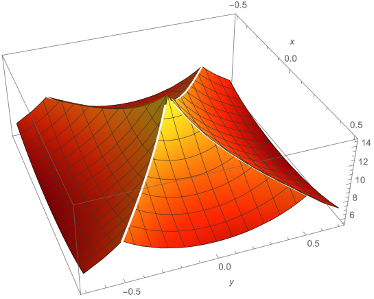
Figure 1: The function used to plot the above figure is $H(x+y)e^{\psi_{0}e^{(-\mu x-\nu y)}}+H(-x+y)e^{\psi_{0}e^{(\mu x-\nu y)}}+H(x-y)e^{\psi_{0}e^{(-\mu x+\nu y)}}+H(-x-y)e^{\psi_{0}e^{(\mu x+\nu y)}}$ where $H(x)$ is the Heaviside function. The above form of the function allows us to plot the solution in all four quadrants. It represents the density profile in xy-plane in the simpler case corresponding to $A_{2}=0$ in Eq. (23).

3.2 The $\psi$ as Exponential Function in Time

It may be mentioned here that we can also get a mathematically consistent solution by considering,

$$f(t)=e^{\gamma t}$$ (33)

where $\gamma$ is a constant. Then we obtain,

$${\bf B}(x,y,t)=-\frac{cT_{0e}^{\prime}}{e\gamma}(\partial_{y}F,-\partial_{x}F,0)(e^{\gamma t}-1)$$ (34)

The jet-like flow ${\bf v}_{i}$ gets the following form,

$${\bf v}_{i}=\frac{a_{0}}{\gamma}F(x,y,t)(e^{\gamma t}-1)\hat{z}$$ (35)

The source term can be defined as,

$$S(x,y,t)==\gamma n(x,y,t)(e^{\gamma t}\psi_{0}F(x,y,t))=\gamma n\psi$$ (36)

The continuity equations reduce to,

$$\partial_{t}\psi=\gamma\psi$$ (37)

At $t=0$, we obtain,

$$\psi(x,y,0)=F(x,y)$$ (38)

Since density becomes double exponential function of time, therefore the parameter $\gamma$ must be chosen very carefully. Note that in this case, the density $n(x,y,t)$ increases very rapidly with time and this solution can be valid only over an extremely short duration of time. Thus, the choice of step function form of $\psi$ during evolution time seems to be physical, and we will use it to investigate the birth and death of spicules in the next section.

3.3 The $\psi$ Constant in Time

If evolution process of the spicule is ignored, then density function $\psi$ can assumed to be time-independent and Eq. (22) for $f(t)=1$ becomes,

$$\psi(x,y)=F(x,y)$$ (39)

Interesting point is that the created fields ${\bf v}_{i}$ and $\tilde{\bf B}$ turn out to be the linear functions of time and Eqs. (29) and (30) remain valid. In this case, the density becomes constant over time, and the source function vanishes, i.e. $S=0$.

4 Creation and Life Cycle of Spicules

In the solar atmosphere, the temperature first decreases from the surface value $T\simeq 6600\;$K to $T\simeq(4300)\;K$ at an altitude of about $500\;$ km from the surface. Above this altitude, the temperature increases from $T\simeq(4300)\;K$ to $10^{4}\;$ K in the upper chromosphere and then after passing through the thin transition region (TR), the temperature increases rapidly to $T\simeq 8\times 10^{5}\;$K Slemzin et al. (2014). Above the transition region lies the lower corona, where the electron temperature reaches the value of $T\simeq 10^{6}\;$K and its gradient becomes very small. The temperature of ions is about two times higher than that of electrons.

We divide the spicule generation process into three different stages keeping in view the temperature variation in the above-mentioned regions. The first stage is its evolution in the lower chromosphere, where the density hump in the $(x,y)$ coordinates is created due to the plasma dynamics in the presence of constant vertical temperature gradients. The vector force $\nabla\psi\times(\nabla T_{e}+\nabla T_{i})$, produces the ion vorticity that is associated with their vertical flow. We assume that the spicule evolves in a time denoted by $\tau_{ev}$ in this region and leaves after attaining a certain upward velocity. Then it crosses the transition region in a shorter time $\tau_{TR}$, because the acceleration produced in TR is greater due to the larger temperature gradients there. However, we assume, for simpler physical picture, that the process of the formation of density structure attains its completion in the lower chromosphere and does not change with time in TR. After gaining a larger velocity in TR, it enters the corona with the final velocity gained in TR that remains almost constant in the lower corona because the upward acceleration is negligible there compared to the lower regions since $\nabla T_{j}\rightarrow 0$. The smaller downward solar gravitational deceleration $(-g_{\odot})$ plays a role in limiting the height of the structure. The final velocity of the density structure becomes zero in the corona after a time $\tau_{l}$ and this is the life time of the spicule.

Figure 2: Schematic diagram of density hump and its velocity in three different regions of solar atmosphere.

4.1 Evolution in Chromosphere

Let us estimate the magnitudes of the acceleration and velocity of the density hump during its evolution in the chromosphere for $t=0\rightarrow\tau_{ev}$. Let $T_{0e}(z_{1})=4\times 10^{3}\;$K be the electron temperature in the lower chromosphere and $T_{0e}(z_{2})=2\times 10^{4}\;$ K be the electron temperature in the upper chromosphere. We choose the thickness of density structure in chromosphere $h_{ch}=z_{2}-z_{1}=10^{3}\;$km and estimate the approximate electron temperature gradient as,

$$T_{0e}^{\prime}\simeq\frac{T_{0e}(z_{2})-T_{0e}(z_{1})}{h}=(2.2)\times 10^{-20}\;\hbox{K}.$$ (40)

Assuming $T_{0i}\simeq 1.5\;T_{0e}$ for hydrogen plasma $m_{i}=1.67\times 10^{-24}$ $gm$, we obtain,

$$a_{0}=\frac{T_{0i}^{\prime}+T_{0e}^{\prime}}{m_{i}}=(3.29)\times 10^{4}cm/S^{2}$$ (41)

Since $(0.388)\leq F(x,y)\leq(1.386)$ within the the density structure, we consider $\mid F(x,y)\mid\simeq 1$ and hence,

$$(v_{iz})_{ev}\simeq(a_{0}-g_{\odot})\tau_{ev}=a\tau_{ev}$$ (42)

where $g_{\odot}=(2.74)\times 10^{4}$ $cm/s^{2}$ is the solar gravitational acceleration in downward direction and it gives $a\simeq(0.55)\times 10^{4}cm/S^{2}$. We assume $\tau_{ev}=(10)$ $S$ and it gives the velocity gained by the density structure of the order of,

$$(v_{iz})_{ev}=(5.5)\times 10^{4}cm/S$$ (43)

4.2 Velocity Gain in the Transition Region

After creation, the density structure enters into the transition region (TR) where its upward acceleration is enhanced due to larger temperature gradients there. If the electron temperature is assumed to increase from $T_{0e}(z_{2})=2\times 10^{4}\;$ K to $T_{0e}(z_{3})=8\times 10^{5}\;$ K at the point $z_{3}$ (top of TR) while the thickness of this layer is $500\;$ km, the gradient of electron temperature turns out to be $T_{0e}^{\prime}=(2.15)\times 10^{-18}\;$ergs/cm which gives $(a)_{TR}=32\times 10^{5}\;$cm/S². We assume that the form of the density function does not change with time in this region. Since $g_{\odot}<<(a)_{TR}$, therefore, the effect of solar gravitational attraction is neglected. The velocity gained in this region by density structure $F(x,y)$ is estimated using the basic relation of classical mechanics,

$$(v_{iz})_{TR}=(v_{iz})_{ev}+[(a)_{TR}]\tau_{TR}$$ (44)

where $\tau_{TR}$ is the time spent by the spicule density structure in TR and $(v_{iz})_{ev}$ is the initial velocity when it enters into TR from chromosphere. Its final velocity in TR becomes $(v_{iz})_{TR}=(128)\;$ km/s.

4.3 Rise and Fall of the Spicule in the Corona

In corona, the upward acceleration vanishes because $\nabla T_{j}\rightarrow 0$ and the density structure enters into this region with the constant velocity gained in TR i.e. $(v_{iz})_{TR}$. Solar gravity acts in downward direction to reduce its vertical speed. The final velocity in corona ,say $(v_{iz})_{cf}$, becomes zero after the life time of spicule $\tau_{l}$ spent in corona which is much longer than its evolution time and the time spent in TR. Following relation holds in corona,

$$(v_{iz})_{cf}=(v_{iz})_{TR}-g_{\odot}\tau_{l}=0.$$ (45)

In this region, the downward solar acceleration does not allow the spicule to move continuously in the vertical direction. In fact, its velocity decreases very slowly here because $g_{\odot}$ is small. The above relation gives $\tau_{l}\simeq(7.78)$ minutes. From this we can compute the maximum height $H$ of the spicule $H\simeq(2.98)\times 10^{4}\;$km. Both the lifetime $\tau_{l}$ and the height $H$ are in the range of the observed values.

Now, we explain why we used the time spent by the spicule center in the TR $\tau_{TR}=4\;$S. The vertical distance covered by the center point of the spicule with a large upward acceleration is $L_{TR}=500\;$km. Then, the following relation can be used to estimate approximately the time spent by the density point in the TR,

$$(500)km\simeq[(v_{iz})_{TR}]\tau_{TR}+[\frac{1}{2}(a_{0})_{TR}]\tau_{TR}^{2}.$$ (46)

We have already estimated the large upward acceleration in this region $(a)_{TR}=(32)km/s^{2}$, and initial velocity is small, therefore we ignore the first term on right hand side of above equation and use,

$$500\;\hbox{km}\simeq[\frac{1}{2}(a)_{TR}]\tau_{TR}^{2},$$ (47)

which gives $\tau_{TR}\simeq(8)S$. Density structures are created one after the other in the chromosphere until the velocity of the first such structure in the corona becomes zero. At this stage, the formation of the density lump at the bottom of the spicule stops.

Figure 3: Schematic diagram of how the upward velocity of density hump increases slowly in stage-I, gets larger speed in stage-II and finally decreases to zero in corona after lifetime $\tau_{l}$. $\tau_{ev}$ is the time for which the spicule evolves in the chromosphere and $\tau_{TR}$ is the time the spicule spends in the transition region.

5 Discussion

Creation process of spicules and their life cycle have been studied by using exact analytical solutions of two fluid plasma equations in three different regions of the solar atmosphere. There are two interesting questions related to this phenomena; one is how the density structure is created in chromosphere with vertical velocity and the other is why this density structure decays in corona after getting a certain height. The first question is explained by showing that if a spatial density structure in xy plane is created in chromosphere in the presence of linear variation of electron and ion temperatures along the z axis, then a thermodynamic force ${\bf F}_{th}$ is produced along the vertical direction and the local density structure moves upward. These structures are created one after the other in chromosphere and attain a form of a plasma jet; the spicule. Plasma is assumed to be quasi-neutral $n_{e}\simeq n_{i}=n$ in a state of non-equilibrium $T_{e}\neq T_{e}$. The second question has a simple explanation based on the fact that if the density structure has almost constant velocity in corona then the solar gravitation acting in downward direction limits the height of density profile in vertical direction.

To understand the mechanism of spicule creation, it is necessary to consider the development of spatial density profile in a local region of the xy plane within a finite time. The density function $\psi=F(x,y)H(t)$ decays exponentially in space away from the origin $(0,0)$.

The life cycle of the spicule is divided into three stages. In stage I, the spicule takes birth in the chromosphere where the density function $F(x,y)$ with exponential decay away from the origin $(0,0)$ is created with the step function $H(t)$ at $t=0$ while the temperatures vary linearly along the z direction. The upward acceleration becomes greater than the solar gravitational constant $g_{\odot}<a$. The source $S(x,y,t)$ of the density increase has the form of a delta function $\delta(t)$ in time. Ions vorticity $(\nabla\times{\bf v}_{i})$ is created by the time-dependent baro clinic vectors $\nabla n(x,y,t)\times(\nabla T_{e}+\nabla T_{i})$. The generated vorticity requires the ions to flow in a vertical direction, viz. ${\bf v}_{i}=v_{iz}(x,y,t)\hat{\bf z}$. The ion velocity is related to the flow of electrons through Ampere’s law, and hence the plasma jet-like flow along the z-axis is generated during a short time of about $10$ seconds. In stage II, the density hump enters the transition region (TR) where the temperature gradients are large and $g_{\odot}<<a$. After achieving a high speed during its passage through TR in a short time span of about $4$ seconds, the spicule enters the corona, where the temperature gradients are vanishingly small, and it moves upwards with almost constant speed. This is the stage-III of the density structure. The solar gravitational acceleration acting in opposite direction to its motion reduces its vertical speed to zero after a long time $\tau_{l}$, which is the life time of the spicule.

The density profile in the xy plane is shown in Fig. (1). Figure (2) explains schematically the three stages of density hump and its upward movement. In the chromosphere, the density structure takes birth during a finite time and is pushed upward. In TR, it gets larger vertical speed, and in corona this speed becomes almost constant initially and reduces slowly to zero due to the action of downward solar gravitational force. The time spent by the density structure in different regions is shown schematically in Fig. (3). It may be noted that Figs. (2) and (3) represent the behavior of physical quantities, but are not according to physical scales. The estimate of the time spent in the corona is the longest time approximately $8$ minutes, and the height attained by the spicule is approximately $30$ thousand kilo meters. Both height $H$ and life time $\tau_{l}$ depend on the magnitudes of the gradients. By varying the scale lengths of the gradients, one can obtain several different sizes of the density structures. This is a general model which can be applied to investigate several different types of jet-like flows.

References

- Antolin et al. (2021) Antolin, P., Pagano, P., Testa, P., Petralia, A., & Reale, F. 2021, Nature Astronomy, 5, 54
- Aschwanden & Peter (2017) Aschwanden, M. J., & Peter, H. 2017, The Astrophysical Journal, 840, 4
- Bellan (2018) Bellan, P. 2018, Journal of Plasma Physics, 84, 755840501
- Biermann (1950) Biermann, L. 1950, Zeitschrift Naturforschung Teil A, 5, 65
- Bol’shov et al. (1991) Bol’shov, L., Dykhne, A., Kowalski, N., et al. 1991, Handbook of Plasma Physics, North-Holland, New York
- Bose et al. (2021) Bose, S., Joshi, J., Henriques, V. M., & van der Voort, L. R. 2021, Astronomy & Astrophysics, 647, A147
- Brueckner & Jorna (1974) Brueckner, K. A., & Jorna, S. 1974, Reviews of modern physics, 46, 325
- Carlsson et al. (2019) Carlsson, M., De Pontieu, B., & Hansteen, V. H. 2019, Annual Review of Astronomy and Astrophysics, 57, 189
- Curtis (1918) Curtis, H. D. 1918, Publications of Lick Observatory, vol. 13, pp. 55-74, 13, 55
- De Pontieu et al. (2007a) De Pontieu, B., McIntosh, S., Carlsson, M., et al. 2007a, science, 318, 1574
- De Pontieu et al. (2007b) De Pontieu, B., McIntosh, S., Hansteen, V. H., et al. 2007b, Publications of the Astronomical Society of Japan, 59, S655
- Dover et al. (2021) Dover, F. M., Sharma, R., & Erdélyi, R. 2021, The Astrophysical Journal, 913, 19
- Ferrari (1998) Ferrari, A. 1998, Annual Review of Astronomy and Astrophysics, 36, 539
- Goddard et al. (2017) Goddard, C. R., Pascoe, D. J., Anfinogentov, S., & Nakariakov, V. 2017, Astronomy & Astrophysics, 605, A65
- González-Avilés et al. (2017) González-Avilés, J., Guzmán, F., & Fedun, V. 2017, The Astrophysical Journal, 836, 24
- Hollweg (1982) Hollweg, J. V. 1982, The Astrophysical Journal, 257, 345
- Jennison & Das Gupta (1953) Jennison, R., & Das Gupta, M. 1953, Nature, 172, 996
- Kingsep et al. (1990) Kingsep, A., Chukbar, K., Yankov, V., & Kadomtsev, B. 1990, Electron Magnetohydrodynamics, 243
- Klimchuk (2006) Klimchuk, J. A. 2006, Solar Physics, 234, 41
- Kuźma et al. (2017) Kuźma, B., Murawski, K., Zaqarashvili, T., Konkol, P., & Mignone, A. 2017, Astronomy & Astrophysics, 597, A133
- Lazarian (1992) Lazarian, A. 1992, Astronomy and Astrophysics, 264, 326
- Martínez-Sykora et al. (2017) Martínez-Sykora, J., De Pontieu, B., Hansteen, V. H., et al. 2017, Science, 356, 1269
- Martínez-Sykora et al. (2020) Martínez-Sykora, J., Leenaarts, J., De Pontieu, B., et al. 2020, The Astrophysical Journal, 889, 95
- Matsumoto & Shibata (2010) Matsumoto, T., & Shibata, K. 2010, The Astrophysical Journal, 710, 1857
- Mestel (1961) Mestel, L. 1961, Monthly Notices of the Royal Astronomical Society, 122, 473
- Priest (1982) Priest, E. 1982, Solar Magnetohydrodynamics (Dordrecht: D. Reidel Publ. Co.), Ch
- Priest (2014) —. 2014, Magnetohydrodynamics of the Sun (Cambridge University Press)
- Saleem (1996) Saleem, H. 1996, Physical Review E, 54, 4469
- Saleem (1999) —. 1999, Physical Review E, 59, 6196
- Saleem (2007) —. 2007, Physics of plasmas, 14
- Saleem (2010) —. 2010, Physics of Plasmas, 17, 092102
- Saleem (2021) —. 2021, Physics of Plasmas, 28
- Saleem & Saleem (2022) Saleem, H., & Saleem, Z. H. 2022, The Astrophysical Journal, 927, 72
- Scalisi et al. (2021a) Scalisi, J., Oxley, W., Ruderman, M. S., & Erdélyi, R. 2021a, The Astrophysical Journal, 911, 39
- Scalisi et al. (2021b) Scalisi, J., Ruderman, M. S., & Erdélyi, R. 2021b, The Astrophysical Journal, 922, 118
- Secchi (1877) Secchi, A. 1877, Le soleil (Gauthier-Villars)
- Shibata et al. (1982) Shibata, K., Nishikawa, T., Kitai, R., & Suematsu, Y. 1982, Solar Physics, 77, 121
- Slemzin et al. (2014) Slemzin, V., Goryaev, F., & Kuzin, S. 2014, Plasma Physics Reports, 40, 855
- Widrow (2002) Widrow, L. M. 2002, Reviews of Modern Physics, 74, 775
- Woo (1996) Woo, R. 1996, Nature, 379, 321
- Yokoyama & Shibata (1995) Yokoyama, T., & Shibata, K. 1995, Nature, 375, 42