Simulation of Open Quantum Systems via Low-Depth Convex Unitary Evolutions

Abstract

Simulating physical systems on quantum devices is one of the most promising applications of quantum technology. Current quantum approaches to simulating open quantum systems are still practically challenging on NISQ-era devices, because they typically require ancilla qubits and extensive controlled sequences. In this work, we propose a hybrid quantum-classical approach for simulating a class of open system dynamics called random-unitary channels. These channels naturally decompose into a series of convex unitary evolutions, which can then be efficiently sampled and run as independent circuits. The method does not require deep ancilla frameworks and thus can be implemented with lower noise costs. We implement simulations of open quantum systems up to dozens of qubits and with large channel rank.

I Introduction

System-environment interactions play an important role in the dynamics of quantum systems, giving rise to phenomena such as dissipation, decoherence, relaxation, and particle or energy transfer processes Breuer and Petruccione (2007); Head-Marsden et al. (2020). Ideal simulations of open quantum systems on classical computers suffer from exponentially scaling memory and runtime requirements, leaving complex physical systems largely out of reach without major approximations Brown et al. (2010). Using quantum computers, several proposed techniques for simulating open systems exist, with a common theme being to encode the challenging non-unitary dynamics on a larger, dilated Hilbert space Paulsen (2003). Numerous techniques make use of Stinespring dilation Stinespring (1955); Hu et al. (2020), Sz.-Nagy dilation Langer (1972); Schlimgen et al. (2021), and linear combination of unitaries Childs and Wiebe (2012); Suri et al. (2022); Head-Marsden et al. (2021). In practice, this dilation leads to long controlled gate sequences and large ancilla frameworks, both of which are practically at odds with NISQ-oriented applications.

An important subset of open system dynamics is the random-unitary channels, which admit an operator-sum decomposition Sudarshan et al. (1961); Hellwig and Kraus (1970) of the form:

$$\mathcal{E}(\rho)=\sum_{i}p_{i}\left(U_{i}\rho U_{i}^{\dagger}\right),$$ (1)

where $p_{i}$ are probabilities and $U_{i}$ are unitary operators Mendl and Wolf (2009). Random-unitary channels, also known as mixed-unitary, naturally represent many probabilistic processes, including the well-known Pauli channels, and have found widespread utility across quantum information science. In fact, general Markovian processes can be mapped onto effective random-unitary channels through Pauli twirling Dür et al. (2005); Cai and Benjamin (2019) and randomized compiling techniques Wallman and Emerson (2016). They are particularly useful for noise modeling of quantum devices Moueddene et al. (2020); Suzuki et al. (2021), as well as within error correction Terhal (2015) and mitigation Temme et al. (2017) schemes. They have also been implemented in the context of quantum simulations of thermal relaxation Rost et al. (2020); Tolunay et al. (2023). As quantum computers continue to grow in size, efficient simulation of random-unitary channels thus becomes increasingly imperative.

To address this need, we propose a hybrid quantum-classical method for simulating random-unitary channels. Our approach involves classically sampling a channel’s probability distribution $\{p_{i}\}$, and then running a series of corresponding circuits on a quantum computer. Compared to ancilla-based methods, this reduces both the number of qubits and the depth of circuits required, thereby widening the class of simulations feasible on near-term quantum computers. By outlining a practical and efficient algorithm, we seek to enhance both the understanding and utility of random-unitary channels.

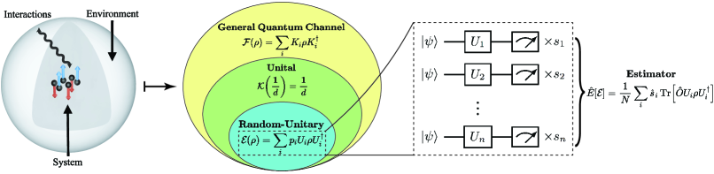
Figure 1: Schematic for simulating random-unitary channels via low-depth convex unitary evolutions. Open system dynamics are described mathematically by their operator-sum representation $\mathcal{F}$, where $K_{i}$ are Kraus operators. Processes which preserve the maximally mixed state are called unital channels, of which random-unitary channels $\mathcal{E}$ are the subset described by Equation 1. An observable $\hat{O}$ of states evolved via random-unitary channels can be simulated via the low-depth, parallel quantum circuits depicted. Here, each circuit corresponding to the unitary $U_{i}$ is simulated with $\mathbb{E}[s_{i}]$ shots, generated from the multinomial distribution $\operatorname{Mult}(N,\{p_{i}\})$. Each measurement is performed with respect to the observable $\hat{O}$, and the results are then aggregated to compute the unbiased estimator $\hat{E}$.

II Random-Unitary Estimation

We present a hybrid quantum-classical method of simulating random-unitary channels for open quantum systems. For an ideal state evolved under a random-unitary channel of the form  (1), $\rho\rightarrow\tilde{\rho}=\mathcal{E}(\rho)$, the expectation value of an observable $\hat{O}$ is:

$$\expectationvalue{\hat{O}}_{\tilde{\rho}} =\operatorname{Tr}\left[\hat{O}\tilde{\rho}\right]$$ (2)

$$=\sum_{i}p_{i}\operatorname{Tr}\left[\hat{O}U_{i}\rho U_{i}^{\dagger}\right].$$ (3)

Typically, ancilla-based methods attempt to faithfully produce $\tilde{\rho}$, which can be accessed directly via measurement.

In our approach, we obtain the above expectation via an estimator of the random-unitary channel, following the formalism of Arrasmith et al. Arrasmith et al. (2020). We generate a multinomial distribution $S\sim\operatorname{Mult}(N,\{p_{i}\})$, with $N$ total number of shots, and $S=(\hat{s}_{1},\hat{s}_{2},\cdot\cdot\cdot\hat{s}_{k})$. The $\hat{s}_{i}$ outcomes correspond to quantum circuits measuring the operator $U_{i}\hat{O}U^{\dagger}_{i}$. Then, the estimator of the expectation values has the form:

$$\hat{E}=\frac{1}{N}\sum_{i}\hat{s}_{i}\operatorname{Tr}\left[\hat{O}U_{i}\rho U^{\dagger}_{i}\right],$$ (4)

where $\mathbb{E}[\hat{s}_{i}]=p_{i}N$. This matches the form of Eq. (2) and is an unbiased estimator. Figure 1 represents this scheme pictorially. The variance of the estimator does not depend on the complexity or size of the random-unitary channel. Rather, it scales with $O(||\hat{O}||/N)$ and is thus efficient up to the operator norm.

We note that a similar heuristic approach was tried for low-dimensional systems, but associated with exponential scaling problems Rost et al. (2020) and was limited to single-qubit applications Tolunay et al. (2023). Crucially, this work demonstrates the feasibility and scalability of this method even for exponentially sized probability distributions $\{p_{i}\}$, as long as this distribution can be sampled efficiently. We demonstrate these ideas for simple open systems which, even in lieu of error mitigation, show constant scaling over an exponential classical problem.

III Demonstrations of Scalable Random-Unitary Simulations

To highlight our approach, we present two cases, both of which lead to exponentially scaling problems. We first look at examples of the depolarizing channel, a Pauli channel which grows exponentially with the number of qubits. We then look at a discretized time-evolution process, which grows exponentially in time. In the first instance, due to the simplicity of the method and the lack of ancilla costs required, we are able to easily demonstrate this approach on superconducting transmon qubit devices. The second example allows for a straightforward demonstration on quantum devices as well, although it can also be classically simulated via exact storage of the two-qubit density matrix.

III.1 Depolarizing Channel

Let $P_{i}^{(n)}$ denote an $n$-qubit Pauli string, i.e. $P_{i}^{(n)}\in\{I,X,Y,Z\}^{\otimes n}$. Then the $n$-qubit depolarizing channel Nielsen and Chuang (2010) can be written as:

$$\mathcal{E}(\rho)=(1-p)\rho+\frac{p}{4^{n}-1}\sum_{i=1}^{4^{n}-1}P_{i}^{(n)}\rho P_{i}^{(n)}.$$ (5)

For $n\in[1,27]$ (with ibmq_montreal having $27$ qubits), we simulate the depolarizing channel on ibmq_montreal with strength parameter $p=0.5$ and an initial state of $|0^{n}\rangle$. For $n\in[1,3]$, we also demonstrate an ancilla-based approach, using a simple linear combination of unitaries. While many such methods exist, we compare simply against the most common example Childs and Wiebe (2012), as generally all of these methods require ancilla circuits. The general resource scaling of the two methods are compared in Table 1. We measure the set of single-Z observables $\langle Z^{(i)}\rangle$, e.g. $Z\otimes I$ for two qubits or $I\otimes Z\otimes I$ for three, and compare to the following analytic result:

$$\langle\hat{Z}^{(i)}\rangle=1-\left(\frac{4^{n}}{4^{n}-1}\right)p.$$ (6)

We plot the mean squared error, ${\rm MSE}=\frac{1}{n}\sum_{i}^{n}(\langle Z^{(i)}\rangle-\langle\hat{Z}^{(i)}\rangle)^{2}$, against the number of qubits for both the ancilla and low-depth methods.

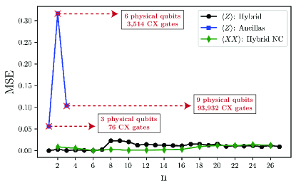
Figure 2: Simulation of the $n$-qubit depolarizing channel on the ibmq_montreal device. The black and blue curves use the starting state of $\left|0^{n}\right\rangle$, and compare the ancilla-based approach to the proposed hybrid sampling method. As suggested by the red $\times$ marks, the ancilla data is shown purely to contrast with the hybrid method. Based on the average errors, the number of CNOTs even for $n=1$ would result in a highly decohered state, so the specific MSE values are not particularly meaningful. The green curve performs the same hybrid simulation but with each pair of qubits prepared in the non-Clifford (NC) starting state $\frac{1}{\sqrt{2}}\ket{00}+\frac{e^{i\pi/4}}{\sqrt{2}}\ket{11}$, and with measurements in the $X$ basis. Each point corresponds to $10^{3}$ shots.

The probabilities associated with each unitary of the depolarizing channel are able to be sampled efficiently. However, due to each of these operations belonging to the Clifford group Gottesman (1998a), this simulation can be classically simulated in polynomial time via the Gottesman-Knill theorem Gottesman (1998b). We also include an instance of a simple non-Clifford state, where we prepare the qubits pairwise in the entangled state $\frac{1}{\sqrt{2}}\ket{00}+\frac{e^{i\pi/4}}{\sqrt{2}}\ket{11}$ and simulate the depolarizing channel for even values of $n$. We measure the set of pairwise observables $\left\langle\hat{X}^{(2i)}\hat{X}^{(2i+1)}\right\rangle$ and compare to the following analytic result:

$$\left\langle\hat{X}^{(2i)}\hat{X}^{(2i+1)}\right\rangle=\frac{1}{\sqrt{2}}\left(1-\left(\frac{4^{n}}{4^{n}-1}\right)p\right).$$ (7)

We plot the mean squared error against the number of simulated qubits using our low-depth hybrid method. All results are combined in Figure 2. As shown, our hybrid sampling method clearly outperforms the traditional ancilla-based approach. It also demonstrates consistently reliable results up to the maximum number of qubits. In contrast, circuits to run the multiplexing operations for the ancilla-based method become infeasible after 3 qubits.

Despite the high numbers of qubits and the prevalence of errors, the simulations here still manage to faithfully capture the simulated state dynamics. In Figure 3, we plot the Hamming weight distribution of the 27-qubit measurements alongside analytic expectation values. Expected bit-flip errors across each qubits skew the results away from the all zero state, yet not in a way that corrupts the overall distribution. We model the overall distribution as the depolarizing channel coupled with bit-flip errors of $p_{X}=4.7\%$ per qubit.

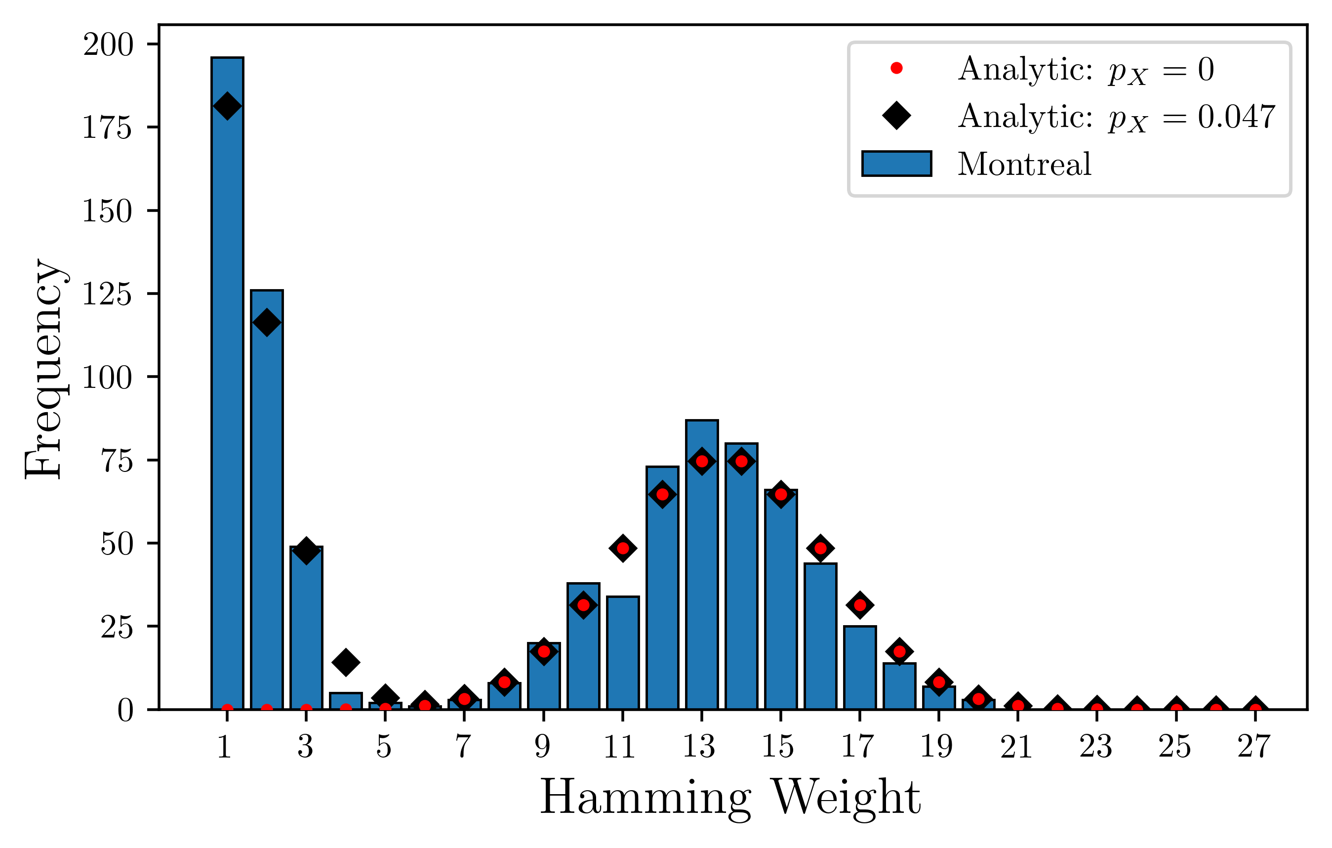
Figure 3: Hamming weight distribution for the 27-qubit depolarizing channel, with starting state $\left|0^{n}\right\rangle$. From the 1000 total measurements, we plot the frequency of each Hamming weight. The blue bars are data from the ibmq_montreal device, the red dots are analytically calculated ideal results, and the black diamonds are analytically calculated results that account for bit-flip errors. The bit-flip effects are most visible at the start of the distribution, as many bit-flip errors symmetrically cancel around the center.

Method	Stinespring	Hybrid
	Dilation	Sampling
Qubits	$n+\lceil\log(m)\rceil$	$n$
Depth	$\Omega(m)$	$1$
Circuits	$1$	$\min(m,N)$
Variance	$\frac{1}{N}\left(\left\langle O^{2}\right\rangle_{\tilde{\rho}}-\left\langle O\right\rangle^{2}_{\tilde{\rho}}\right)$	$\frac{1}{N}\left(\sum_{i}p_{i}\left\langle O^{2}\right\rangle_{\tilde{\rho_{i}}}-\langle O\rangle_{\tilde{\rho}}^{2}\right)$

Table 1: Comparison of resources used in simulating $n$-qubit quantum channels, comprised of a convex sum of $m$ unitary evolutions.

III.2 Noisy Hamiltonian Evolution

To look at the performance under a different exponentially propagating scheme, we simulate the two-qubit transverse-field Ising model (TFIM) under a noise channel which occurs at each discretized step.

The TFIM Hamiltonian is

$$H=-J\sigma_{z}^{(1)}\sigma_{z}^{(2)}-h\left(\sigma_{x}^{(1)}+\sigma_{x}^{(2)}\right),$$ (8)

where $J$ is the exchange interaction parameter and $h$ quantifies the strength of the transverse magnetic field. For small time steps $\Delta t$, we evolve this system as the Hamiltonian propagator composed with random-unitary channel $\mathcal{S}$. The resulting composed operator is itself a random-unitary channel, denoted as $\tilde{\mathcal{S}}$. We generate each time step recursively, by sampling a distribution as in Eq. (4):

$$\tilde{\mathcal{S}}_{t+1}=\tilde{\mathcal{S}}\circ\tilde{\mathcal{S}}_{t}.$$ (9)

We simulate these dynamics on the ibmq_kolkata device, with a depolarizing strength of $p=0.05$ per time step, and with TFIM parameters $J=1$ and $h=1$. Figure 4 shows the populations over time, both in the standard computational basis and in the eigenbasis of the Hamiltonian. Fitting exponential decay functions to the eigenstate population curves yields an estimated decoherence time of $T_{1}=4.84\pm 0.46$ (a.u.), encompassing the predicted time of $T_{1}=5.25$ (a.u.).

In this example, the possible number of circuits to sample from grows exponentially with the number of time steps. For our simulations, after 25 time steps there are $16^{25}$ circuit permutations to consider, a seemingly intractable sample space. However, due to the constant norm of the probability distribution vector, the measurement statistics are agnostic to the complexity of the sample space. This enables our results to accurately capture the system-environment dynamics while using only $10^{3}$ shots at each time point.

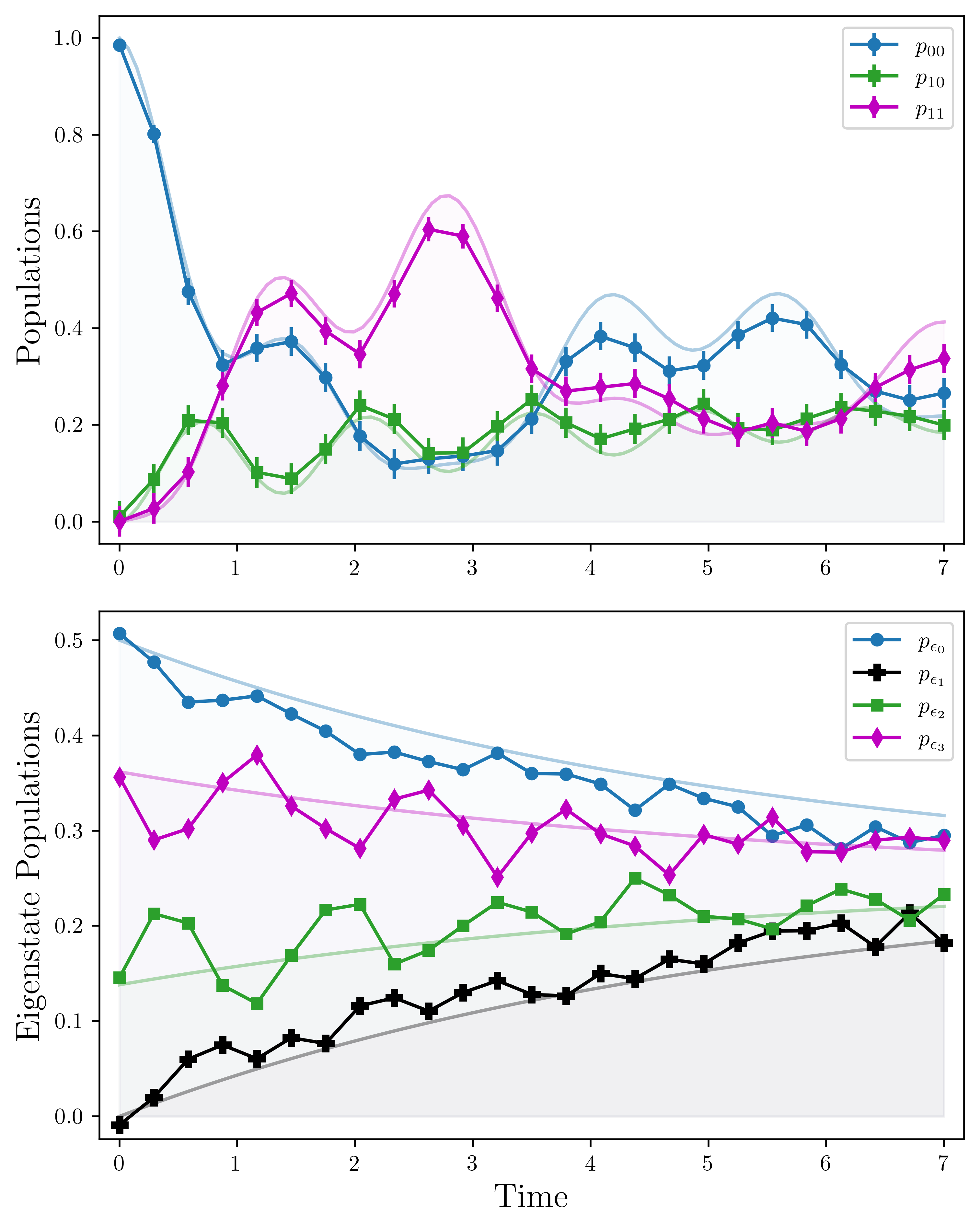
Figure 4: Simulation of the two-qubit TFIM subject to depolarizing noise. The points represent data from ibmq_kolkata, and the smooth curves represent the analytic results. The top figure displays populations over time in the standard basis, while the bottom figure displays populations in the eigenbasis of the TFIM Hamiltonian. Note that analytically $p_{01}(t)=p_{10}(t)$, so we omit $p_{01}(t)$ for visual clarity.

IV Discussion and Conclusion

These results demonstrate that for a certain class of quantum channels, we can obtain a significant benefit via the proposed hybrid quantum-classical approach. By delegating unitary transformations to the quantum device, exponentially complex processes can potentially be handled efficiently and are combined through classical sampling and processing.

This advantage is clearly seen against the ancilla-based method, although there is at least one limitation. Even though our method is more efficient, it does not prepare a coherent quantum state as an output. This means that any observables obtained via further evolutions of the state must also be processed through an estimator. For instance, if one wishes to use a mixed state as input to some broader algorithm, then any desired observables at the end of this algorithm must themselves be sampled using an estimator of the form in Equation 4. However, if the channel’s Stinespring circuit has an exponential number of compiled gates, implementation via any quantum processor will likely be significantly challenging as well. This problem is demonstrated in Figure 2, where simulating 3 qubits with dilation techniques requires nearly $10^{5}$ CX gates.

We point out that our method joins a prolific space of stochastic techniques within quantum simulation, and open quantum systems in particular. This is evidenced by many of the aforementioned works Wallman and Emerson (2016); Moueddene et al. (2020); Suzuki et al. (2021); Terhal (2015); Temme et al. (2017); Rost et al. (2020); Tolunay et al. (2023). Stochastic compilation methods have also notably been used to construct first-order dynamics of Hamiltonian evolution Campbell (2019) and twirled channels Kim et al. (2023), and as a tool in implementing certain shallow channels Rost et al. (2020).

Other difficulties exist in practically implementing these simulations on quantum computers. For instance, random distributions that cannot be sampled in constant or polynomial time could themselves result in memory issues. Another problem exists for $U_{i}$ that cannot be efficiently implemented as products of two-qubit unitaries, i.e. unitaries with exponential complexity in their generators, although this does not exclude their generation via more sophisticated quantum simulators. These problems would also plague ancilla-based approaches. Finally, while the generality of the method in the context of the entire operator space is quite limited, for random-unitary channels the proposed method offers a straightforward approach for simulating complex dynamics.

Modeling environmental effects are essential in understanding the dynamics of many physical systems. The current work proposes a straightforward way to simulate random-unitary noise channels via classical probabilistic sampling of low-depth unitaries. For quantum simulations of random-unitary processes, the proposed hybrid approach has clear advantages over ancilla-based techniques. While the scope is limited to random-unitary channels, these represent an important class of quantum channels, opening the door for a variety of other dynamics to be simulated on near-term quantum devices.

V Acknowledgements

This work is supported by the NSF RAISE-QAC-QSA, Grant No. DMR-2037783; the Department of Energy, Office of Basic Energy Sciences, Grant No. DE-SC0019215; the NSF DGE NRT-QISE, Grant No. 2125924; the NSF ECCS CAREER, Grant No. 1944085; and the NSF CNS, Grant No. 2247007.

The authors acknowledge the use of IBM Quantum services for this work. The views expressed are those of the authors, and do not reflect the official policy or position of IBM or the IBM Quantum team.

VI Appendix

VI.1 Shot Allocation

While the hybrid simulation method laid out in Section I is robust to different sampling schemes, we optimize the use of valuable computing resources with shot-frugal allocation methods. Practically, some of the operators within a random-unitary channel demand higher priority due to their different weightings $p_{i}$ in Equation 2. Throughout these results, we use weighted random sampling of the probability distributions $\{p_{i}\}$ to allocate shots, thus optimizing the use of computing time Arrasmith et al. (2020). More precisely, we sample the operator space $\{U_{i}\}$ with corresponding probabilities $\{p_{i}\}$ to determine the circuit run for each shot. This means that for a simulation using a total of $N$ shots, on average $p_{i}N$ shots will be allocated to each operator $U_{i}$ within the sampled space.

To compute the variance of our estimator in Equation 4, we follow the weighted random sampling calculations of Arrasmith et al. Arrasmith et al. (2020). This gives the following variance:

$$\operatorname{Var}(\hat{E})=\frac{1}{N}\left(\sum_{i}p_{i}\left\langle O^{2}\right\rangle_{\tilde{\rho_{i}}}-\langle O\rangle_{\tilde{\rho}}^{2}\right),$$ (10)

where $\tilde{\rho_{i}}:=U_{i}\rho U_{i}^{\dagger}$. In comparison, when using Stinespring dilation, the variance of the estimator $\hat{E}_{S}$ is simply $\frac{1}{N}$ times the variance of the expectation value $\expectationvalue{O}_{\tilde{\rho}}$:

$$\operatorname{Var}(\hat{E}_{S})=\frac{1}{N}\left(\left\langle O^{2}\right\rangle_{\tilde{\rho}}-\left\langle O\right\rangle^{2}_{\tilde{\rho}}\right).$$ (11)

Analytically, these expressions are equivalent: Applying Equation 2 to $O^{2}$ yields $\expectationvalue{O^{2}}_{\tilde{\rho}}=\sum_{i}p_{i}\left\langle O^{2}\right\rangle_{\tilde{\rho_{i}}}$. However, our hybrid sampling can only provide access to the individual expectation values $\left\langle O^{2}\right\rangle_{\tilde{\rho_{i}}}$, making Equation 10 the practical means of calculating the variance.

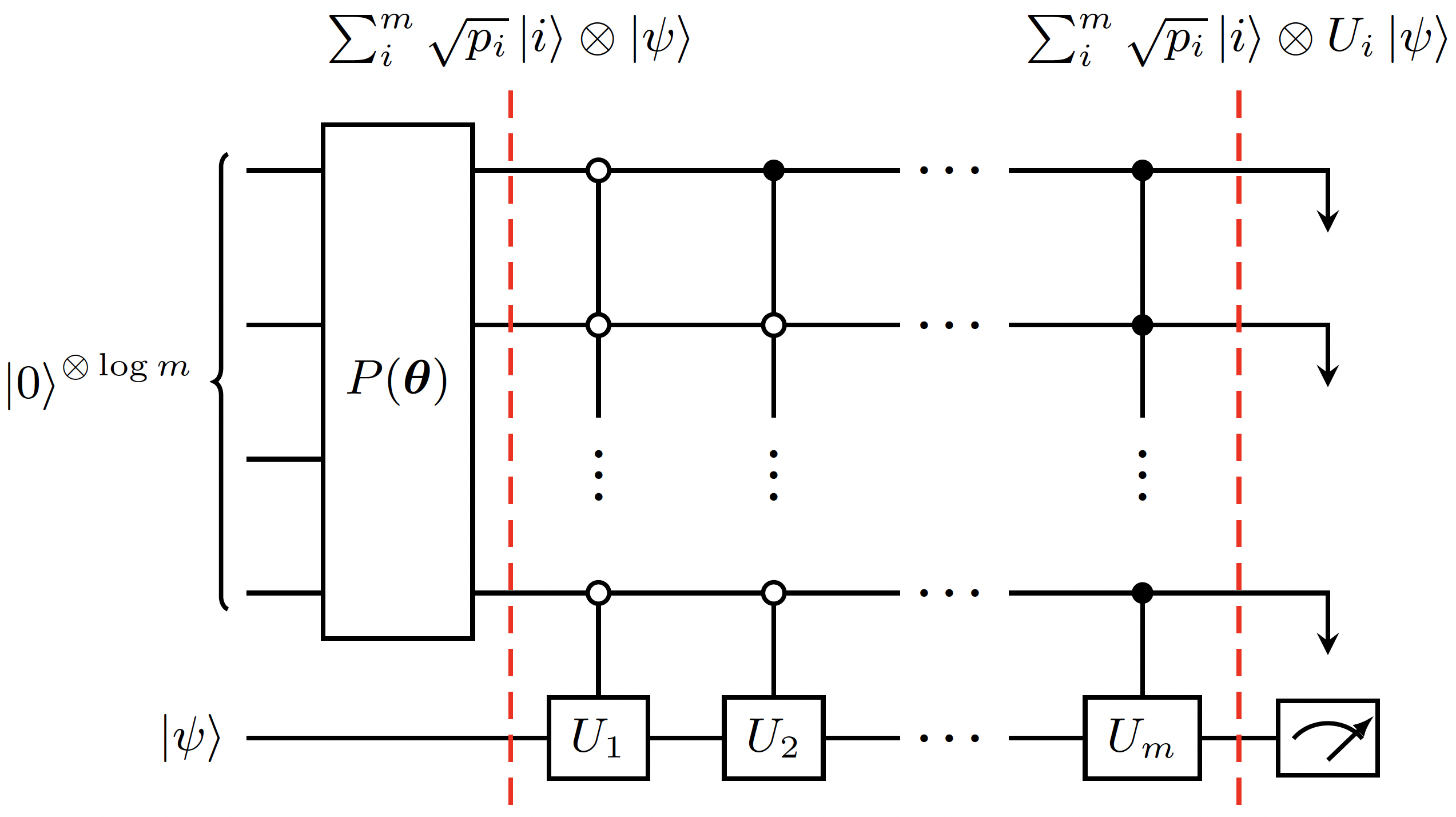
Figure 5: Circuit schematic for ancilla-based simulation method Childs and Wiebe (2012). The state of the combined ancilla-target system is displayed above each red, dotted line.

VI.2 Analytic Expectation Values

The $n$-qubit depolarizing channel in Equation 5 can equivalently be written as follows Nielsen and Chuang (2010):

$$\mathcal{E}(\rho)=(1-\lambda)\rho+\lambda\frac{I}{2^{n}},$$

where $\lambda=(\frac{4^{n}}{4^{n}-1})p$. This form greatly simplifies analytic calculations, and in fact the expectation value of a general observable $\hat{O}$ evolved under $\mathcal{E}$ can be calculated as follows:

$$\expectationvalue{\hat{O}}_{\tilde{\rho}}=(1-\lambda)\operatorname{Tr}\left[O\rho\right]+\frac{\lambda}{2^{n}}\operatorname{Tr}\left[O\right].$$ (12)

From this form, we computed the analytic expectation values $\langle\hat{Z}^{(i)}\rangle$ and $\left\langle\hat{X}^{(2i)}\hat{X}^{(2i+1)}\right\rangle$ in Equations 6 and 7 respectively.

VI.3 Ancilla-Based Algorithm

For the depolarizing channel simulations, we compare with results from an ancilla-based simulation algorithm Childs and Wiebe (2012), described as follows. Consider the random-unitary channel $\mathcal{E}(\rho)=\sum_{i}^{m}p_{i}\left(U_{i}\rho U_{i}^{\dagger}\right)$. First, encode the probabilities $p_{i}$ as amplitudes of $\lceil\log(\mathrm{m})\rceil$-many ancilla qubits. Suppose a gate $P(\bm{\theta})$ exists such that:

$$P(\bm{\theta})\ket{0^{\lceil\log(\mathrm{m})\rceil}}=\sum_{i}^{m}\sqrt{p_{i}}\ket{i}.$$ (13)

Then, apply each unitary evolution $U_{i}$ to the target state $\ket{\psi}$ conditioned on the ancilla state $\ket{i}$. This accomplishes the desired effect of applying each unitary $U_{i}$ with probability $p_{i}$. The overall algorithm is displayed in circuit-form in Figure 5.

References

- Breuer and Petruccione (2007) Heinz-Peter Breuer and Francesco Petruccione, The Theory of Open Quantum Systems (Oxford University Press, Oxford, New York, 2007).
- Head-Marsden et al. (2020) Kade Head-Marsden, Johannes Flick, Christopher J. Ciccarino, and Prineha Narang, “Quantum Information and Algorithms for Correlated Quantum Matter,” Chemical Reviews (2020), 10.1021/acs.chemrev.0c00620.
- Brown et al. (2010) Katherine L. Brown, William J. Munro, and Vivien M. Kendon, “Using Quantum Computers for Quantum Simulation,” Entropy 12, 2268–2307 (2010).
- Paulsen (2003) Vern Paulsen, Completely Bounded Maps and Operator Algebras, Cambridge Studies in Advanced Mathematics (Cambridge University Press, Cambridge, 2003).
- Stinespring (1955) W. Forrest Stinespring, “Positive functions on c*-algebras,” in Proceedings of the American Mathematical Society, Vol. 6 (1955) pp. 211–216.
- Hu et al. (2020) Zixuan Hu, Rongxin Xia, and Sabre Kais, “A quantum algorithm for evolving open quantum dynamics on quantum computing devices,” Scientific Reports 10, 3301 (2020).
- Langer (1972) H. Langer, “B. Sz.-Nagy and C. Foias, Harmonic Analysis of Operators on Hilbert Space. VIII + 387 S. Budapest/Amsterdam/London 1970. Akadémiai Kiadó/North-Holland Publishing Company,” ZAMM - Zeitschrift für Angewandte Mathematik und Mechanik 52, 501–501 (1972).
- Schlimgen et al. (2021) Anthony W. Schlimgen, Kade Head-Marsden, Leeann M. Sager, Prineha Narang, and David A. Mazziotti, “Quantum Simulation of Open Quantum Systems Using a Unitary Decomposition of Operators,” Physical Review Letters 127, 270503 (2021), arxiv:2106.12588 .
- Childs and Wiebe (2012) Andrew M. Childs and Nathan Wiebe, “Hamiltonian simulation using linear combinations of unitary operations,” Quantum Information & Computation 12, 901–924 (2012).
- Suri et al. (2022) Nishchay Suri, Joseph Barreto, Stuart Hadfield, Nathan Wiebe, Filip Wudarski, and Jeffrey Marshall, “Two-Unitary Decomposition Algorithm and Open Quantum System Simulation,” (2022), arXiv:2207.10007 [physics, physics:quant-ph].
- Head-Marsden et al. (2021) Kade Head-Marsden, Stefan Krastanov, David A. Mazziotti, and Prineha Narang, “Capturing non-Markovian dynamics on near-term quantum computers,” Physical Review Research 3, 013182 (2021).
- Sudarshan et al. (1961) E. C. G. Sudarshan, P. M. Mathews, and Jayaseetha Rau, “Stochastic Dynamics of Quantum-Mechanical Systems,” Physical Review 121, 920–924 (1961).
- Hellwig and Kraus (1970) K. E. Hellwig and K. Kraus, “Operations and measurements. II,” Communications in Mathematical Physics 16, 142–147 (1970).
- Mendl and Wolf (2009) Christian B. Mendl and Michael M. Wolf, “Unital Quantum Channels – Convex Structure and Revivals of Birkhoff’s Theorem,” Communications in Mathematical Physics 289, 1057–1086 (2009).
- Dür et al. (2005) W. Dür, M. Hein, J. I. Cirac, and H.-J. Briegel, “Standard forms of noisy quantum operations via depolarization,” Physical Review A 72, 052326 (2005).
- Cai and Benjamin (2019) Zhenyu Cai and Simon C. Benjamin, “Constructing Smaller Pauli Twirling Sets for Arbitrary Error Channels,” Scientific Reports 9, 11281 (2019).
- Wallman and Emerson (2016) Joel J. Wallman and Joseph Emerson, “Noise tailoring for scalable quantum computation via randomized compiling,” Physical Review A 94, 052325 (2016).
- Moueddene et al. (2020) Ahmed Abid Moueddene, Nader Khammassi, Koen Bertels, and Carmen G. Almudever, “Realistic simulation of quantum computation using unitary and measurement channels,” Physical Review A 102, 052608 (2020).
- Suzuki et al. (2021) Yasunari Suzuki, Yoshiaki Kawase, Yuya Masumura, Yuria Hiraga, Masahiro Nakadai, Jiabao Chen, Ken M. Nakanishi, Kosuke Mitarai, Ryosuke Imai, Shiro Tamiya, Takahiro Yamamoto, Tennin Yan, Toru Kawakubo, Yuya O. Nakagawa, Yohei Ibe, Youyuan Zhang, Hirotsugu Yamashita, Hikaru Yoshimura, Akihiro Hayashi, and Keisuke Fujii, “Qulacs: a fast and versatile quantum circuit simulator for research purpose,” Quantum 5, 559 (2021), arXiv:2011.13524 [physics, physics:quant-ph].
- Terhal (2015) Barbara M. Terhal, “Quantum Error Correction for Quantum Memories,” Reviews of Modern Physics 87, 307–346 (2015), arXiv:1302.3428 [quant-ph].
- Temme et al. (2017) Kristan Temme, Sergey Bravyi, and Jay M. Gambetta, “Error Mitigation for Short-Depth Quantum Circuits,” Physical Review Letters 119, 180509 (2017).
- Rost et al. (2020) Brian Rost, Barbara Jones, Mariya Vyushkova, Aaila Ali, Charlotte Cullip, Alexander Vyushkov, and Jarek Nabrzyski, “Simulation of Thermal Relaxation in Spin Chemistry Systems on a Quantum Computer Using Inherent Qubit Decoherence,” (2020), arXiv:2001.00794 [physics, physics:quant-ph].
- Tolunay et al. (2023) Meltem Tolunay, Ieva Liepuoniute, Mariya Vyushkova, and Barbara A. Jones, “Hamiltonian simulation of quantum beats in radical pairs undergoing thermal relaxation on near-term quantum computers,” Phys. Chem. Chem. Phys. 25, 15115–15134 (2023).
- Arrasmith et al. (2020) Andrew Arrasmith, Lukasz Cincio, Rolando D. Somma, and Patrick J. Coles, “Operator Sampling for Shot-frugal Optimization in Variational Algorithms,” (2020), arXiv:2004.06252 [quant-ph].
- Nielsen and Chuang (2010) Michael A. Nielsen and Isaac L. Chuang, “Quantum Computation and Quantum Information: 10th Anniversary Edition,” (2010).
- Gottesman (1998a) Daniel Gottesman, “Theory of fault-tolerant quantum computation,” Physical Review A 57, 127–137 (1998a).
- Gottesman (1998b) Daniel Gottesman, “The Heisenberg Representation of Quantum Computers,” (1998b), arXiv:quant-ph/9807006.
- Campbell (2019) Earl Campbell, “Random Compiler for Fast Hamiltonian Simulation,” Physical Review Letters 123, 070503 (2019).
- Kim et al. (2023) Youngseok Kim, Christopher J. Wood, Theodore J. Yoder, Seth T. Merkel, Jay M. Gambetta, Kristan Temme, and Abhinav Kandala, “Scalable error mitigation for noisy quantum circuits produces competitive expectation values,” Nat. Phys. 19, 752–759 (2023).