Parameter-Free FISTA by Adaptive Restart and Backtracking

Abstract

We consider a combined restarting and adaptive backtracking strategy for the popular Fast Iterative Shrinking-Thresholding Algorithm [11] frequently employed for accelerating the convergence speed of large-scale structured convex optimization problems. Several variants of FISTA enjoy a provable linear convergence rate for the function values $F(x_{n})$ of the form $\mathcal{O}(e^{-K\sqrt{\mu/L}\leavevmode\nobreak\ n})$ under the prior knowledge of problem conditioning, i.e. of the ratio between the (Łojasiewicz) parameter $\mu$ determining the growth of the objective function and the Lipschitz constant $L$ of its smooth component. These parameters are nonetheless hard to estimate in many practical cases. Recent works address the problem by estimating either parameter via suitable adaptive strategies. In our work both parameters can be estimated at the same time by means of an algorithmic restarting scheme where, at each restart, a non-monotone estimation of $L$ is performed. For this scheme, theoretical convergence results are proved, showing that a $\mathcal{O}(e^{-K\sqrt{\mu/L}n})$ convergence speed can still be achieved along with quantitative estimates of the conditioning. The resulting Free-FISTA algorithm is therefore parameter-free. Several numerical results are reported to confirm the practical interest of its use in many exemplar problems.

1 Introduction

The Fast Iterative Soft-Thresholding Algorithm (FISTA) has been popularized in the work of Beck and Teboulle [11] as an extension of previous works by Nesterov [33, 34] where improved $O(1/n^{2})$ convergence rate was shown upon suitable extrapolation of the algorithmic iterates. In [34], such rate is shown to be optimal for the class of convex functions, outperforming the one of the classical Forward-Backward algorithm [19]. In its vanilla form, FISTA is indeed an efficient strategy for computing solutions of convex optimization problems of the form

$$\min_{x\in\mathbb{R}^{N}}\leavevmode\nobreak\ F(x):=f(x)+h(x),$$ (1.1)

where $F:\mathbb{R}^{N}\to\mathbb{R}\cup\left\{+\infty\right\}$ belongs to $\mathcal{H}_{L}$, the class of composite functions with $f$ convex and differentiable with $L$-Lipschitz gradient and $h$ convex, proper and lower semicontinuous (l.s.c.) with simple (i.e. easily computable) proximal operator. We also assume: $X^{*}:=\operatorname*{arg\,min}_{x}\leavevmode\nobreak\ F(x)\neq\emptyset$.

Due to its wide use in many areas of signal/image processing, many extensions of FISTA enjoying monotonicity [10], general extrapolation rules [4], inexact proximal point evaluations [42], variable metrics [14] and improved $o(1/n^{2})$ convergence rate [5] were proposed along with a large number of FISTA-type algorithms addressing specific features (e.g., FASTA [24], Faster-FISTA [29] to name a few). The question on the convergence of iterates of FISTA was solved in [17] whose results were then further investigated in several other papers, see, e.g., [28, 29]. The algorithmic convergence of FISTA relies on an upper bound on the algorithmic step-size, which depends on the inverse of the Lipschitz constant $L$. Practically, the estimation of $L$ may be pessimistic and/or costly, which may result in unnecessary small step-size values. To avoid this, several backtracking strategies have been proposed based either on monotone (Armijo-type) [11] or adaptive updates [41].

Interestingly, when the function $F$ satisfies additional growth assumptions such as strong convexity or quadratic growth, first-order methods may provide improved convergence rates. Under such hypotheses, Heavy-Ball type methods provide the fastest convergence rates. Such methods rely on a constant-in-time inertial coefficient which is chosen according to $\kappa=\frac{\mu}{L}$ where $\mu>0$ is the parameter appearing in the growth condition. In fact, $\kappa$ is the inverse of the condition number and knowing its value is crucial for these methods to reach rates of the form $\mathcal{O}\left(e^{-K\sqrt{\kappa}n}\right)$ for some real constant $K>0$. We refer the reader to [6, Table 2] for further details and comparisons. Note that in such a setting the Forward-Backward method guarantees in fact a decay of the error in $\mathcal{O}\left(e^{-\kappa n}\right)$ which is much slower since $\kappa\ll 1$ in general. Different approaches requiring the explicit prior knowledge of both strong convexity parameters $\mu_{f}$ and $\mu_{h}$ of the functions in (1.1) have been studied in [18, 15, 22] and endowed with possible adaptive backtracking strategies.

In [7] it has been shown that unlike Heavy-Ball methods, FISTA does not significantly benefit from growth-type assumptions. The presence of an inertial coefficient growing with the iterations amplifies the effect of inertia, so the scheme can generate oscillations when the function $F$ is sharp. From a theoretical viewpoint, the decay of the error cannot be better than polynomial although the finite-time behavior of FISTA is close to the one of Heavy-Ball methods. Restarting FISTA for functions satisfying some growth condition is a natural way of controlling inertia, which allows to accelerate the overall convergence. The main idea consists in reinitializing to zero the inertial coefficient based on some restarting condition. Elementary computations show that by restarting every $k^{*}$ iterations for some $k^{*}$ depending on $\sqrt{\kappa}$, the worst-case convergence improves to $\mathcal{O}\left(e^{-K\sqrt{\kappa}\leavevmode\nobreak\ n}\right)$ for some $K>0$ [43, 21, 31]. Nonetheless, such restarting rule requires the knowledge of $\kappa$ and provides slower worst-case guarantees than Heavy-Ball methods. On the other hand, adaptive restarting techniques allow the adaptation of the inertial parameters to $F$ without requiring any knowledge on its geometry (apart from $L$). In [37], the authors propose heuristic restart rules based on rules involving the values of $F$ or $\nabla F$ at each iterate. These schemes are efficient in practice as they do not require any estimate of $\kappa$, but they do not enjoy any rigorous convergence rate. Fercoq and Qu introduce in [20] a restarting scheme achieving a fast exponential decay of the error when only a (possibly rough) estimate of $\mu$ is available. In [3, 1, 2], Alamo et al. propose strategies ensuring linear convergence rates only using information on $F$ or the composite gradient mapping at each iterate. Roulet and d’Aspremont propose in [40] a restarting scheme based on a grid-search strategy providing a fast decay as well. Note that by restarting FISTA an estimate of the growth parameter can be done as shown by Aujol et al. in [8], where fast linear convergence is shown.

Adaptive methods exploiting the geometry of $F$ without knowing its growth parameter $\mu$ are useful in practice since estimating $\mu$ is generally difficult. In the same spirit, numerical schemes for strongly convex functions where the growth parameter is unknown are provided by Nesterov in [35, Section 5.3] and by Gonzaga and Karas in [25]. In the case of strongly convex objectives, Lin and Xiao introduced in [30] an algorithm achieving a fast exponential decay of the error by automatically estimating both $L$ and $\mu$ at the same time.

In this paper we consider a parameter-free FISTA algorithm (called Free-FISTA) with provable accelerated linear convergence rates of the form $\mathcal{O}(e^{-K\sqrt{\kappa}n})$ for functions satisfying the quadratic growth condition:

$$(\exists\mu>0)\quad\text{s.t.}\quad(\forall x\in\mathbb{R}^{N})\quad\frac{\mu}{2}d(x,X^{*})^{2}\leq F(x)-F^{*},$$ (1.2)

assuming that both the growth parameter $\mu>0$ and the Lipschitz smoothness parameter $L>0$ of $\nabla f$ are unknown. By a suitable combination of existing previous work combining an adaptive restarting strategy for the estimation of $\mu$ [8] and a non-monotone estimation of $L$ performed via adaptive backtracking at each restart [41, 15], Free-FISTA adapts its parameters to the local geometry of the functional $F$, thus resulting in an effective performance on several exemplar problems in signal and image processing. The proposed strategy relies on an estimate ${\kappa}_{j}$ of $\kappa$ which is rigorously showed to provide a restarting rule that guarantees fast convergence.

2 Preliminaries and notations

We are interested in solving the convex, non-smooth composite optimization problem (1.1) under the following assumptions:

• The function $f:\mathbb{R}^{N}\to\mathbb{R}_{+}$ is convex, differentiable with $L$-Lipschitz gradient:

  $$(\exists L\geq 0)\quad(\forall x,y\in\mathbb{R}^{N})\quad\|\nabla f(x)-\nabla f(y)\|\leq L\|x-y\|.$$

• The function $h:\mathbb{R}^{N}\to\mathbb{R}_{+}\cup\left\{+\infty\right\}$ is proper, l.s.c. and convex. Its proximal operator will be denoted by:

  $$\text{prox}_{h}(z)=\operatorname*{arg\,min}_{w\in\mathbb{R}^{N}}\leavevmode\nobreak\ h(w)+\frac{1}{2}\|w-z\|^{2},\quad z\in\mathbb{R}^{N}.$$ (2.1)

For this class of functions a classical minimization algorithm is the Forward-Backward algorithm (FB) whose iterations are described by:

$$x_{k+1}=\text{prox}_{\tau h}(x_{k}-\tau\nabla f(x_{k})),\quad\tau\in\left(0,\frac{2}{L}\right).$$

To define in a compact way the Forward-Backward iteration performed on $y\in\mathbb{R}^{N}$ with a step-size $\tau>0$, we will use the notation $T_{\tau}(y)=\text{prox}_{\tau h}(y-\tau\nabla f(y)).$ while for assessing optimality via a suitable stopping criterion, we will consider a condition of the form $0\in\partial F(y)$, or, equivalently, $g_{\tau}(y)=0$ with the composite gradient mapping being defined by:

$$g_{\tau}(y):=\frac{y-T_{\tau}(y)}{\tau}=\frac{1}{\tau}\left(y-\text{prox}_{\tau h}\left(y-\tau\nabla f(y)\right)\right),\quad y\in\mathbb{R}^{N}.$$

This last formulation is convenient for defining an approximate solution to the composite problem, and thus to deduce a tractable stopping criterion:

Definition 1 ($\varepsilon$-solution)

Let $\varepsilon>0$ and $\tau>0$. An iterate $y\in\mathbb{R}^{N}$ is said to be an $\varepsilon$-solution of the problem (1.1) if: $\|g_{\tau}(y)\|\leqslant\varepsilon$.

Given an estimation $\hat{L}>0$ of $L$ and a tolerance $\varepsilon>0$, the exit condition considered will then read $\|g_{1/\hat{L}}(y)\|\leqslant\varepsilon$. As a shorthand notation, we also define the class of functions satisfying (1.2):

Definition 2 (Functions with quadratic growth, $\mathcal{G}_{\mu}^{2}$)

Let $F:\mathbb{R}^{N}\rightarrow\mathbb{R}\cup\{+\infty\}$ be a proper l.s.c. convex function with $X^{*}:=\operatorname*{arg\,min}\leavevmode\nobreak\ F\neq\emptyset$. Let $F^{*}:=\inf F$. The function $F$ satisfies a quadratic growth condition $\mathcal{G}_{\mu}^{2}$ for some $\mu>0$ if:

$$(\forall x\in\mathbb{R}^{N}),\qquad\frac{\mu}{2}d(x,X^{*})^{2}\leqslant F(x)-F^{*}.$$ (2.2)

Condition (2.2) can be seen as a relaxation of strong convexity. As shown in [13, 23] in a convex setting such condition is equivalent to a global Łojasiewicz property with an exponent $\frac{1}{2}$. In particular, the following lemma states an implication that is required in the later sections.

Lemma 1

Let $F:\mathbb{R}^{N}\rightarrow\mathbb{R}\cup\{+\infty\}$ be a proper, l.s.c. and convex function with a non-empty set of minimizers $X^{*}$. Let $F^{*}=\inf F$. If $F$ satisfies $\mathcal{G}^{2}_{\mu}$ for some $\mu>0$, then $F$ has a global Łojasiewicz property with an exponent $\frac{1}{2}$:

$$(\forall x\in\mathbb{R}^{N}),\quad\frac{\mu}{2}\left(F(x)-F^{*}\right)\leqslant d(0,\partial F(x))^{2}.$$

3 Free-FISTA

In this paper we propose a parameter-free restart algorithm based on the original FISTA scheme proposed by Beck and Teboulle in [10]:

$$y_{k}=x_{k}+\frac{t_{k}-1}{t_{k+1}}(x_{k}-x_{k-1}),\quad x_{k+1}=\text{prox}_{\tau h}(y_{k}-\tau\nabla f(y_{k})),$$

where the sequence $(t_{k})_{k\in\mathbb{N}}$ is recursively defined by: $t_{1}=1$ and $t_{k+1}=(1+\sqrt{1+4t_{k}^{2}})/{2}$. For the class of convex composite functions, the convergence rate of the method is given by [33, 10]:

$$(\forall k\in\mathbb{N}),\quad F(x_{k})-F^{*}\leqslant\frac{2L\|x_{0}-x^{*}\|^{2}}{(k+1)^{2}}.$$

When $L$ is available, a classical strategy introduced in [32] is to restart the algorithm at regular intervals. Necoara and al. [31] propose an optimized restart scheme, proving that restarting Nesterov accelerated gradient every $\lfloor 2e\sqrt{\frac{L}{\mu}}\rfloor$ iterations ensures that $F(x_{k})-F^{*}=\mathcal{O}\left(e^{-\frac{1}{e}\sqrt{\frac{\mu}{L}}k}\right)$ for the class of $\mu$-strongly convex functions. This restart scheme and its convergence analysis can be extended to composite functions satisfying some quadratic growth condition $\mathcal{G}^{2}_{\mu}$ [37, 31].

In this paper we consider the case when both the Lipschitz constant $L$ and the growth parameter $\mu$ are unknown. The first main ingredient of our parameter-free FISTA algorithm is the use of an adaptive backtracking strategy used at each restart to provide a non-monotone estimation of the local Lipschitz constant $L$. More precisely, we propose a backtracking variant of FISTA (FISTA-BT), widely inspired by the one proposed in [15] and described in Section 3.1. The second main ingredient is an adaptative restarting approach, described in Section 3.2, taking advantage of the local estimation of the geometry of $F$ (via online estimations of the parameter $\kappa=\frac{\mu}{L}$) for avoiding oscillations due to inertia. The main steps of Free-FISTA are the following: at each restart, given a current iterate $r_{j-1}$, a fixed number of iterations $n_{j-1}$ and a current estimation $L_{j-1}^{+}$ of the Lipschitz constant $L$,

1. Compute $r_{j}$ a new iterate and $L_{j}$ a new estimation of $L$ by performing $n_{j-1}$ iterations of FISTA-BT algorithm parameterized by the estimate $L_{j-1}^{+}$.

2. Compute an estimation $\kappa_{j}$ of the geometric parameter $\kappa=\frac{\mu}{L}$.

3. Update the number $n_{j}$ of iterations of FISTA-BT for the next restart loop. It depends on $n_{j-1}$ and on $\kappa_{j}$.

The whole algorithm is carefully described in Section 3.3 and its convergence is proven. All technical proofs are reported in a dedicated Appendix A.

3.1 Adaptive backtracking

In order to provide at each restart of Free-FISTA an estimation of $L$ adapted to the current estimate of the growth parameter, we describe in the following an instance of FISTA endowed with non-monotone backtracking previously considered, e.g., in [41, Algorithm 2] and [15, Algorithm 2] with $\mu=0$. Differently from standard approaches following an Armijo-type (i.e. monotone) backtracking rule [11], the use of a non-monotone strategy further allows for a local decreasing of the estimated valued $\hat{L}$ of $L$ (equivalently, an increasing of $\tau$ w.r.t. to the optimal $1/L$) in the neighborhoods of “flat” points of the function $f$ (i.e. where $L$ is small), thus improving practical performances.

Following [15], the proposed adaptive backtracking strategy is derived from the classical descent condition holding for FISTA at ${x}^{+}:=T_{\tau}(x)$ with $x\in\mathbb{R}^{N}$, which reads: for any $y\in\mathbb{R}^{N}$,

$$F(x^{+})+\frac{\|y-x^{+}\|^{2}}{2\tau}+\left(\frac{\|x^{+}-x\|^{2}}{2\tau}-D_{f}(x^{+},x)\right)\leq F(y)+\frac{\|y-x^{+}\|^{2}}{2\tau},$$ (3.1)

which is defined in terms of the Bregman divergence $D_{f}:\mathbb{R}^{N}\times\mathbb{R}^{N}\to\mathbb{R}_{+}$ associated to $f$ and defined by: $D_{f}(x,y)=f(x)-f(y)-\langle\nabla f(y),x-y\rangle.$ Choosing $y=x$ in (3.1), the descent of $F$ between two iterates $x$ and $x^{+}=T_{\tau}(x)$ is at least of:

$$F(x^{+})-F(x)\leqslant-\frac{\|x^{+}-x\|^{2}}{2\tau},\quad\text{provided that}\quad D_{f}(x^{+},x)\leq\frac{\|{x}^{+}-{x}\|^{2}}{2\tau}.$$ (3.2)

This last condition is true whenever $0<\tau\leq 1/L$. When only a local estimate $L_{k}$ of $L$ is available, the idea is to enforce (3.2) by applying a backtracking strategy t by $\tau_{k}=\frac{1}{L_{k}}$: testing a tentative step-size $\tau_{k}=\tau_{k-1}/\delta$ with $\delta\in(0,1)$ greater than the one $\tau_{k-1}$ considered at the previous iteration, decrease the step $\tau_{k}$ by a factor $\rho\in(0,1)$ as long as condition (3.2) is not satisfied. This condition can be rewritten as $\frac{2D_{f}(x^{+},x)}{\|x^{+}-x\|^{2}}>\frac{\rho}{\tau_{k}}=\rho L_{k}$, where $\tau_{k}/\rho$ denotes the last step before acceptance. Note that by the condition above, for all $k\geq 0$ there holds:

$$\tau_{k}\geq\frac{\rho}{L}\qquad\Leftrightarrow\qquad L_{k}\leq\frac{L}{\rho},$$ (3.3)

which can be used to get the desired convergence result.

The algorithm FISTA_adaBT is reported in Algorithm 1.

Algorithm 1 FISTA + adaptive backtracking, FISTA_adaBT($x^{0},n,L_{0},L_{min};\rho,\delta$)

Initializations: $\tau_{0}=1/L_{0}$, $\rho\in(0,1),\delta\in(0,1]$, $x_{-1}=x_{0}\in\mathcal{X}$, $t_{0}=1$, $L_{min}$ sufficiently small.

for $k=0,1,\ldots,n$ do

$$\tau^{0}_{k+1}=\min\left\{\frac{\tau_{k}}{\delta},\frac{1}{L_{min}}\right\};$$ (3.4)

  $i=0;$

  repeat

$$\tau_{k+1} =\rho^{i}\leavevmode\nobreak\ \tau^{0}_{k+1};$$

$$t_{k+1} =\frac{1+\sqrt{1+4\frac{\tau_{k}}{\tau_{k+1}}t^{2}_{k}}}{2};$$ (3.5)

$$\beta_{k+1} =\frac{t_{k}-1}{t_{k+1}};$$

$$y_{k+1} =x_{k}+\beta_{k+1}(x_{k}-x_{k-1});$$

$$x_{k+1} =\text{prox}_{\tau_{k+1}h}(y_{k+1}-\tau_{k+1}\nabla f(y_{k+1}));$$

$$i =i+1;$$

until  $D_{f}(x_{k+1},y_{k+1})\leq\|x_{k+1}-y_{k+1}\|^{2}/2\tau_{k+1}$

end forReturn $(x_{k+1},L_{k+1}=\frac{1}{\tau_{k+1}})$

The parameter $L_{min}>0$ provides a lower bound of the estimated Lipschitz constants at any $k$, i.e $L_{k}=\frac{1}{\tau_{k}}\geqslant L_{min}$. This property will be needed to prove the theoretical asymptotic convergence rate of the global restarting scheme. Such parameter has to satisfy the condition $L_{min}<L$. However, since this value should be taken as small as possible this condition is not restrictive and it practically does not affect the choice (3.4). We observe that whenever $\delta<1$, the increasing of the algorithmic step-size is attempted at each outer iteration of Algorithm 1, while, when $\delta=1$, the same value $\tau_{k}$ estimated at the previous iterations is used. In both cases, a standard Armijo-type backtracking is then run to adjust possible over-estimations.

Convergence of Algorithm 1 is stated in the following Theorem, which is a special case of [15, Theorem 4.6] suited for the particular case $\mu=0$ (no strong-convexity).

Theorem 1 (Convergence of Algorithm 1 [15])

Let $n\in\mathbb{N}$. The sequence $(x_{k})_{k=0,\dots,n}$ generated by the Algorithm 1 satisfies for all $k=0,\ldots,n$:

$$F(x_{k+1})-F^{*}\leq\frac{2\bar{L}_{k+1}}{(k+1)^{2}}\|x_{0}-x^{*}\|^{2},$$ (3.6)

where, by setting $L_{i}:=1/\tau_{i}$ the quantity $\bar{L}_{k+1}$ is defined by:

$$\bar{L}_{k+1}:=\left(\frac{1}{\frac{1}{k+1}\sum_{i=1}^{k+1}\frac{1}{\sqrt{L_{i}}}}\right)^{2}.$$ (3.7)

The (harmonic) average appearing in (3.6) depends only on the estimates of $L$ performed along the iterations of Algorithm 1. In particular, it does not depend on the unknown value of the Lipschitz constant $L$. However, recalling (3.3), we have for all $k=1,\dots,n$, $\rho\bar{L}_{k+1}\leqslant L$, hence the following bound:

$$\frac{2\bar{L}_{k+1}}{(k+1)^{2}}\leq\frac{2L}{\rho(k+1)^{2}}$$ (3.8)

which, plugged in (3.6), entails the well-known convergence rate for FISTA endowed with Armijo-type backtracking showed, e.g., in [11].

Remark 1

Regarding the choice of the extrapolation rule (3.5), we remark that in [8] a different update based on [17] was considered to guarantee the convergence of the iterates of the resulting FISTA scheme. Since the convergence result in Theorem 1 cannot be adapted to this different choice in a straightforward manner, we consider in this work a Nesterov-type update, inspired by previous work [41, 15].

We can now state the main proposition (whose proof is detailed in Section A.1) which will be used in the following to formulate the proposed adaptive restarting strategy described in Section 3.2:

Proposition 1

Let $F$ be a function satisfying $\mathcal{H}_{L}$ and $\mathcal{G}^{2}_{\mu}$ for some $L>0$ and $\mu>0$. If $L_{min}\in[0,L)$, then for any fixed $n\in\mathbb{N}^{*}$, the sequence $(x_{k})_{k=0\dots n}$ provided by Algorithm 1 satisfies for all $k\in\mathbb{N}$:

(i) $$\leavevmode\nobreak\ \ F(x_{k+1})-F^{*}\leqslant\frac{4L}{\rho\mu(k+1)^{2}}\left(F(x_{0})-F^{*}\right),$$ (3.9)

(ii) $$\leavevmode\nobreak\ F(x_{k+1})\leqslant F(x_{0}),$$ (3.10)

3.2 Adaptive restarting

Having provided an estimate of $L$ after one algorithmic restart $j\geq 1$, intuitively, let us now describe the strategy of Free-FISTA. The structure of the algorithm relies on two main ingredients: a tractable stopping criterion suitable to cope with the hypothesis that the Lipschitz constant $L$ is not available, and a strategy to approximate the unknown value of the conditioning parameter $\kappa=\frac{\mu}{L}$ by a sequence $(\kappa_{j})_{j}$ whose values will be needed to define the number $n_{j}$ of inner FISTA-BT iterations to be performed at each restart.

3.2.1 A tractable stopping criterion

Let $\varepsilon>0$ be the expected accuracy and $(r_{j},L_{j})$ be the $j-th$ output of Algorithm 1 for $n_{j-1}$ iterations at the $j-th$ restart. When the Lipschitz constant $L$ is available, the notion of $\varepsilon$-solution can be seen as a good stopping criterion for an algorithm solving the composite optimization problem for three reasons: first it is numerically quantifiable. Secondly controlling the norm of the composite gradient mapping is roughly equivalent to having a control on the values of the objective function. Lastly, it will enable to analyze and compare algorithms in terms of the number of iterations needed to reach the accuracy $\varepsilon$.

Algorithm 2 Forward-Backward step with Armijo-backtracking, FB_BT($r,L_{0};\rho$)

Require: $r\in\mathbb{R}^{N}$, $L_{0}>0$, $\rho\in(0,1)$. $i=0$

repeat$\tau=\frac{\rho^{i}}{L_{0}}$ ${r}^{+}=T_{\tau}(r)$ $i=i+1$

until $D_{f}(r^{+},r)\leqslant\|r^{+}-r\|^{2}/2\tau$

Return $r^{+},\leavevmode\nobreak\ L^{+}=\frac{L_{0}}{\rho^{i-1}}$

When only estimations $L_{j}$ of $L$ are available at each restart, there is no guarantee that the condition $\|g_{1/L_{j}}(r_{j})\|\leqslant\varepsilon$ will enable to control the values of the objective functions. To get a tractable stopping criterion, we propose to add a Forward-Backward step with Armijo backtracking before the next restart. Such an algorithm, denoted by FB_BT, is detailed in Algorithm 2. This extra step ensures that the following condition holds for all $j\geqslant 1$:

$$D_{f}({r}_{j}^{+},r_{j})\leqslant\frac{{L}_{j}^{+}}{2}\|{r}_{j}^{+}-r_{j}\|^{2},$$ (3.11)

where $({r}_{j}^{+}=T_{1/{L}_{j}^{+}}(r_{j}),{L}_{j}^{+})$ denote the outputs of Algorithm 2, and $g_{1/L_{j}^{+}}(r_{j})=L_{j}^{+}(r_{j}-r_{j}^{+})$ with, by construction: $L_{j}^{+}\geqslant L_{j}$. Note that the computational cost of the composite gradient mapping $g_{1/L_{j}^{+}}(r_{j})$ is therefore very low. The stopping criterion of Free-FISTA thus reads:

$$\|g_{1/L_{j}^{+}}(r_{j})\|\leqslant\varepsilon.$$ (3.12)

The condition (3.12) is a “good” stopping criterion in the sense that it enables to control the values of the objective function along the iterations. Our analysis relies on the following Lemma whose proof is detailed in Section A.3:

Lemma 2

Let $F$ be a function satisfying $\mathcal{H}_{L}$ and $\mathcal{G}^{2}_{\mu}$ for some $L>0$ and $\mu>0$. Then for all $x\in\mathbb{R}^{N}$ and $\tau>0$ we have:

$$F(T_{\tau}(x))-F^{*}\leqslant\frac{2(1+L\tau)^{2}}{\mu}\|g_{\tau}(x)\|^{2}.$$

Applying Lemma 2 to the iterate $r_{j}$, we get:

$$F({r}_{j}^{+})-F^{*}\leqslant\frac{2(1+L/{L}_{j}^{+})^{2}\varepsilon^{2}}{\mu},$$

where, importantly, does not require the computation of $F^{*}$. In addition, remembering that the parameter $L_{min}\in\left(0,L\right)$ from Algorithm 1 provides a lower bound on the estimates $L_{j}$ and that $L_{j}^{+}\geqslant L_{j}$, we necessarily have: $L_{j}^{+}\geqslant L_{min}$ and thus:

$$F({r}_{j}^{+})-F^{*}\leqslant\frac{2(1+L/L_{min})^{2}\varepsilon^{2}}{\mu}.$$

Remark 2

An alternative choice for ${L}_{j}$ following from (3.6) is ${L}_{j}=\bar{L}_{j}$ with

$$\bar{L}_{j}=\left(\frac{1}{\frac{1}{n_{j-1}}\sum_{k=1}^{n_{j-1}}\frac{1}{\sqrt{L_{k}}}}\right)^{2}$$

being the average (3.7) estimated at the $j$-the restart. Nonetheless, we prefer ${L}_{j}=\frac{1}{\tau_{n_{j-1}}}\leqslant\frac{L}{\rho}$, as the last estimation of $L$ at the $j$-th restart approximates the local smoothness of the functional. Moreover, its value is in general smaller than the value $\bar{L}_{j}$, which, when used for the next call of Algorithm 1 is expected to require fewer adjustments, thus improving the overall efficiency.

3.2.2 Estimating the geometric paramater $\kappa$

Once the stopping criterion is well defined, the next issue is to determine the number of FISTA-BT iterations to perform at each restart. The global principle of our restart scheme is as follows: at the $j$-th restart,

• Compute $(r_{j},L_{j})=\mbox{FISTA\_adaBT}(r_{j-1}^{+},n_{j-1},L_{j-1}^{+},L_{min};\rho,\delta)$ where $r_{j}$ is the iterate computed after $n_{j-1}$ iterations of FISTA_adaBT and $L_{j}$ the associated estimate of the Lipschitz constant $L$.

• Perform an extra step of backtracking Forward-Backward:

  $$(r_{j}^{+},L_{j}^{+})=\mbox{FB\_BT}(r_{j},L_{j};\rho).$$

• Update the number of iterations $n_{j}$ for the next restart.

Inspired by [8], the update of the number $n_{j}$ of iterations relies on the estimation of the inverse $\kappa=\frac{\mu}{L}$ of the conditioning at each restart loop by comparing the values $F(r_{j})-F^{*}$ and $F(r_{j-1})-F^{*}$ at each restart $j$. More precisely, applying the first claim of Proposition 1 at the $j$-th restart, we have: for all $j\in\mathbb{N}^{*}$

$$F(r_{j})-F^{*} \leqslant \frac{4L}{\rho\mu(n_{j-1}+1)^{2}}\left(F(r_{j-1}^{+})-F^{*}\right)\leqslant\frac{4L}{\rho\mu(n_{j-1}+1)^{2}}\left(F(r_{j-1})-F^{*}\right),$$

observing that by the property (3.11), we have: $F(r_{j}^{+})\leqslant F(r_{j})$ as explained in Section 3.1. We thus deduce:

$$(\forall j\in\mathbb{N}^{*}),\quad\kappa\leqslant\frac{4}{\rho(n_{j-1}+1)^{2}}\frac{F(r_{j-1})-F^{*}}{F(r_{j})-F^{*}}.$$ (3.13)

Since $F^{*}$ is often not known in practice and noticing that the application $u\mapsto\frac{F(r_{j-1})-u}{F(r_{j})-u}$ is non decreasing on $[F^{*},F(r_{j})]$ (since $F(r_{j})\leqslant F(r_{j-1})$), we deduce:

$$(\forall j\in\mathbb{N}^{*}),\quad\kappa\leqslant\frac{4}{\rho(n_{j-1}+1)^{2}}\frac{F(r_{j-1})-F(r_{j+1})}{F(r_{j})-F(r_{j+1})}.$$

Using such inequality, it is thus possible to get a sequence $\left(\kappa_{j}\right)_{j}$ estimating $\kappa$ at each restart $j\geqslant 2$ by comparing $F(r_{j-1})-F(r_{j})$ and $F(r_{j-2})-F(r_{j})$ by defining:

$$(\forall j\geqslant 2),\quad\kappa_{j}:=\min\limits_{\underset{i<j}{i\in\mathbb{N}^{*}}}\leavevmode\nobreak\ \frac{4}{\rho(n_{i-1}+1)^{2}}\frac{F(r_{i-1})-F(r_{j})}{F(r_{i})-F(r_{j})}.$$ (3.14)

By construction the sequence $(\kappa_{j})_{j\in\mathbb{N}}$ is non-increasing along the iterations :

Lemma 3

Let $F$ be a function satisfying $\mathcal{H}_{L}$ and $\mathcal{G}^{2}_{\mu}$ for some $L>0$ and $\mu>0$. Then the sequence $(\kappa_{j})_{j\geqslant 2}$ defined by (3.14) satisfies

$$(\forall j\geqslant 2),\quad\kappa_{j}\geqslant\kappa_{j+1}>\kappa.$$ (3.15)

3.3 Free-FISTA: structure and convergence results

Free-FISTA is detailed in Algorithm 3. Note that the ‘free’ dependence on parameters stressed here relates to the two smoothness and growth parameters, $L$ and $\mu$, respectively. The hyperaparameters $\rho\in(0,1)$, $\delta\in(0,1]$, $L_{min}>0$ required by Free-FISTA to perform adaptive backtracking and to assess the expected precision ($0<\varepsilon\ll 1$) do not affect its convergence properties.

Algorithm 3 Free-FISTA: parameter-free FISTA with adaptive backtracking and restart

require: $r_{0}\in\mathbb{R}^{N}$, $j=1$, $L_{0}>0$, $L_{min}>0$, $\rho\in(0,1)$, $\delta\in(0,1]$, $0<\varepsilon\ll 1$ $n_{0}=\lfloor 2C\rfloor$ $(r_{1},{L}_{1})=$FISTA_adaBT$(r_{0},n_{0},L_{0},L_{min};\rho,\delta)$ $n_{1}=\lfloor 2C\rfloor$ $({r}_{1}^{+},{L}_{1}^{+})=\text{{FB\_BT}}(r_{1},{L}_{1};\rho)$

repeat $j=j+1$ $(r_{j},{L}_{j})=$FISTA_adaBT$({r}_{j-1}^{+},n_{j-1},{L}_{j-1}^{+},L_{min};\rho,\delta)$ ${\kappa}_{j}=\min_{i<j}\leavevmode\nobreak\ \frac{4}{\rho(n_{i-1}+1)^{2}}\frac{F(r_{i-1})-F(r_{j})}{F(r_{i})-F(r_{j})}$

     if $n_{j-1}\leq C\sqrt{\frac{1}{{\kappa}_{j}}}$ then $n_{j}=2n_{j-1}$

     else$n_{j}=n_{j-1}$

     end if$({r}_{j}^{+},L_{j}^{+})=\text{{FB\_BT}}(r_{j},{L}_{j};\rho)$

until $\|g_{1/L_{j}^{+}}(r_{j})\|\leqslant\varepsilon$

return $r={r}_{j}^{+}$

To summarize, Free-FISTA Algorithm 3 relies on a few sequences:

• the sequence $(r_{j})_{j\in\mathbb{N}}$ corresponds to the (outer/global) iterates. For all $j>0$, $r_{j}$ is the output of the $j$-th execution of Algorithm 1 after one extra application of Algorithm 2.

• the sequence $(n_{j})_{j\in\mathbb{N}}$ refers to the number of estimated iterations of Algorithm 1 to be performed at the $j$-th restart. For all $j\geqslant 0$ we thus have:

  $$(r_{j+1},{L}_{j})=\text{{FISTA\_adaBT}}({r}_{j}^{+},n_{j};{L}_{j}^{+},L_{min};\rho,\delta),$$

  where $(r_{j}^{+},L_{j}^{+})$ is obtained after an extra Forward-Backward step with backtracking applied to $(r_{j},L_{j})$.

• the sequence $({L}_{j})_{j}$ estimating $L$ at each restart.

• the sequence $(\kappa_{j})_{j\geqslant 2}$ estimating at each restart the true problem conditioning $\kappa=\mu/L$ by comparing the cost function $F$ at three different iteration points.

Let us finally explain our strategy to update the number $n_{j}$ of iterations required by Algorithm 1 at the $j$-th restart. Once an estimate $\kappa_{j}$ is computed, the strategy performed by Free-FISTA consists in updating $n_{j}$ using a doubling condition that depends on a parameter $C>0$ to be defined:

$$n_{j-1}\leq C\sqrt{\frac{1}{{\kappa}_{j}}}$$ (3.16)

Thus, Free-FISTA checks whether such condition is fulfilled: if it holds true, then $n_{j-1}$ is considered too small and doubled so that $n_{j}=2n_{j-1}$. Otherwise, the number of iterations is kept unchanged. By construction, the sequence $(n_{j})_{j\in\mathbb{N}}$ is non-decreasing, and satisfies the following lemma.

Lemma 4

Let $F$ be a function satisfying $\mathcal{H}_{L}$ and $\mathcal{G}^{2}_{\mu}$ for some $L>0$ and $\mu>0$. Then the sequence $(n_{j})_{j\in\mathbb{N}}$ provided by Algorithm 3 satisfies

$$\forall j\in\mathbb{N},\quad n_{j}\leqslant 2C\sqrt{\frac{1}{\kappa}}.$$

Note that for all $j\geqslant 2$, the number of iterations $n_{j}$ is defined according to $n_{j-1}$, $\kappa_{j}$ and the predefined parameter $C>0$. The proof of Lemma 4 is straightforward by induction: first observe that $n_{0}=\lfloor 2C\rfloor\leqslant 2C\leqslant 2C\sqrt{\frac{1}{\kappa}}$. Assume that $n_{j-1}\leqslant 2C\sqrt{1/\kappa}$. By construction, either (3.16) is satisfied and $n_{j}=2n_{j-1}\leqslant 2C\sqrt{\frac{1}{\kappa_{j}}}\leqslant 2C\sqrt{\frac{1}{\kappa}},$ by monotonicity of $(\kappa_{j})_{j\in\mathbb{N}}$ (see Equation 3.15), or (3.16) is not satisfied, and $n_{j}=n_{j-1}\leqslant 2C\sqrt{1/\kappa}$ by assumption.

We can now state the main convergence results of Free-FISTA. Their proof can be found in Section A.5 and Section A.6, respectively.

Theorem 2

Let $F$ be a function satisfying $\mathcal{H}_{L}$ and $\mathcal{G}^{2}_{\mu}$ for some $L>0$ and $\mu>0$. Let $(r_{j})_{j\in\mathbb{N}}$ and $(n_{j})_{j\in\mathbb{N}}$ be the sequences provided by Algorithm 3 with parameters $C>4/\sqrt{\rho}$ and $\varepsilon>0$. Then, the number of iterations $1+\sum_{i=0}^{j}n_{i}$ required to guarantee $\|g_{1/{L}_{j}^{+}}(r_{j})\|\leqslant\varepsilon$ is bounded and satisfies

$$\sum_{i=0}^{j}n_{i}\leqslant\frac{4C}{\log\left(\frac{C^{2}\rho}{4}-1\right)}\sqrt{\frac{L}{\mu}}\left(2\log\left(\frac{C^{2}\rho}{4}-1\right)+\log\left(1+\frac{16}{C^{2}\rho-16}\frac{2L(F(r_{0})-F^{*})}{\rho\varepsilon^{2}}\right)\right).$$

Corollary 1

Let $F$ be as above. If $C>4/\sqrt{\rho}$, $\varepsilon>0$ and $L_{min}\in(0,L)$, then the sequences $(r_{j})_{j\in\mathbb{N}}$ and $(n_{j})_{j\in\mathbb{N}}$ provided by Algorithm 3 satisfy

$$F({r}_{j}^{+})-F^{*}=\mathcal{O}\left(e^{-\frac{\log\left(\frac{C^{2}\rho}{4}-1\right)}{4C}\sqrt{\kappa}\displaystyle\sum_{i=0}^{j}n_{i}}\right).$$

Moreover, the trajectory of total number of FISTA iterates has a finite length and the method converges to a minimizer $x^{*}\in X^{*}$.
Specifically, if $C$ maximizes $\frac{\log\left(\frac{C^{2}\rho}{4}-1\right)}{4C}$, namely $C\approx 6.38/\sqrt{\rho}$, then there exists $K>\frac{1}{12}$ such that the sequences $(r_{j})_{j\in\mathbb{N}}$ and $(n_{j})_{j\in\mathbb{N}}$ satisfy

$$F({r}_{j}^{+})-F^{*}=\mathcal{O}\left(e^{-\sqrt{\rho}K\sqrt{\kappa}\displaystyle\sum_{i=0}^{j}n_{i}}\right).$$

Corollary 1 states that the Free-FISTA algorithm 3 provides asymptotically a fast exponential decay. This convergence rate is consistent with the one expected for functions $F$ satisfying $\mathcal{H}_{L}$ and $\mathcal{G}^{2}_{\mu}$ where both the parameters $L$ and $\mu$ are unknown a priori. Note that in this setting Forward-Backward algorithm provides a low exponential decay The variation of Heavy-Ball method introduced in [6], the FISTA restart scheme introduced in [20] and fixed restart of FISTA require to estimate the growth parameter to ensure a fast exponential decay. FISTA algorithm has the same fast decay as Free-FISTA in finite time (see [7]), but with a smaller constant.

4 Numerical experiments

In this section, we report several applications of the Free-FISTA Algorithm 3 showing how an automatic estimation of the smoothness parameter $L$ and the growth parameter $\mu$ can be beneficial. The combined approach is compared with vanilla FISTA [11], FISTA with restart [8] and FISTA with adaptive backtracking (Algorithm 1) [15]. The first two examples show the advantages of Free-FISTA in comparison with other schemes, while the last example highlights some existing limitations of restarting methods. The codes that generate the figures are available in the following GitHub repository: https://github.com/HippolyteLBRRR/Benchmarking_Free_FISTA.git

4.1 Logistic regression with $\ell^{2}$-$\ell^{1}$-regularization

As a first example, we focus on a classification problem defined in terms of a given dictionary $A\in\mathbb{R}^{m\times n}$ and labels $b\in\left\{-1,1\right\}^{m}$. We consider the minimization problem:

$$\min_{x\in\mathbb{R}^{n}}\leavevmode\nobreak\ F(x):=\underbrace{\frac{\lambda_{1}}{2\|A^{T}b\|_{\infty}}\sum_{j=1}^{m}\log\left(1+e^{-b_{j}a_{j}^{T}x}\right)+\frac{\lambda_{2}}{2}\|x\|^{2}}_{:=f(x)}+\underbrace{\|x\|_{1}}_{:=h(x)},$$ (4.1)

where $a_{j}=(A_{i,j})_{j}\in\mathbb{R}^{m}$ is the $j$-th row of $A$, $\lambda_{1}>0$ and $\lambda_{2}>0$. By definition, the value $x^{*}$ minimizing $F$ is expected to satisfy $\mathbb{P}(b_{i}=1|a_{i})=\frac{1}{1+e^{-a_{i}^{T}x^{*}}}$ for any $i\in\llbracket 1,m\rrbracket$. Note that the $\ell^{2}$ term aims to smooth the objective function while the $\ell^{1}$ regularization sparsfies the solution which helps preventing from overfitting. An upper estimation of $L$ can easily be computed:

$$\hat{L}=\frac{\lambda_{1}\|A^{T}b\|^{2}}{8\|A^{T}b\|_{\infty}}+\lambda_{2},$$ (4.2)

which may be large whenever $\|A^{T}b\|\gg 1$. We note that the function $F$ satisfies the assumption $\mathcal{G}^{2}_{\mu}$ for some growth parameter $\mu>0$ whose estimation is not straightforward. We solve this problem for a randomly generated dataset with $n=30000$ and $m=100$. We compare the following methods:

• FISTA [11] with a fixed stepsize $\tau=\frac{1}{\hat{L}}$;

• FISTA restart [8] with a fixed stepsize $\tau=\frac{1}{\hat{L}}$,

• FISTA_adaBT (Algorithm 1) with $\rho=0.8$ and $\delta=0.95$,

• Free-FISTA (Algorithm 3) with $\rho=0.8$ and $\delta=0.95$.

We set $\lambda_{1}=10$, $\lambda_{2}=3$ and $x_{0}\leftarrow\mathcal{U}\left([-1,1]\right)$. We get that $\hat{L}\geqslant 9\cdot 10^{5}$ is an upper bound of $L$. An estimate of the solution of (4.1) is pre-computed by running Free-FISTA for a large number of iterations. This allows us to compute for all methods $\log\left(F(r_{j})-\hat{F}\right)$ with $\hat{F}\approx F^{*}$.

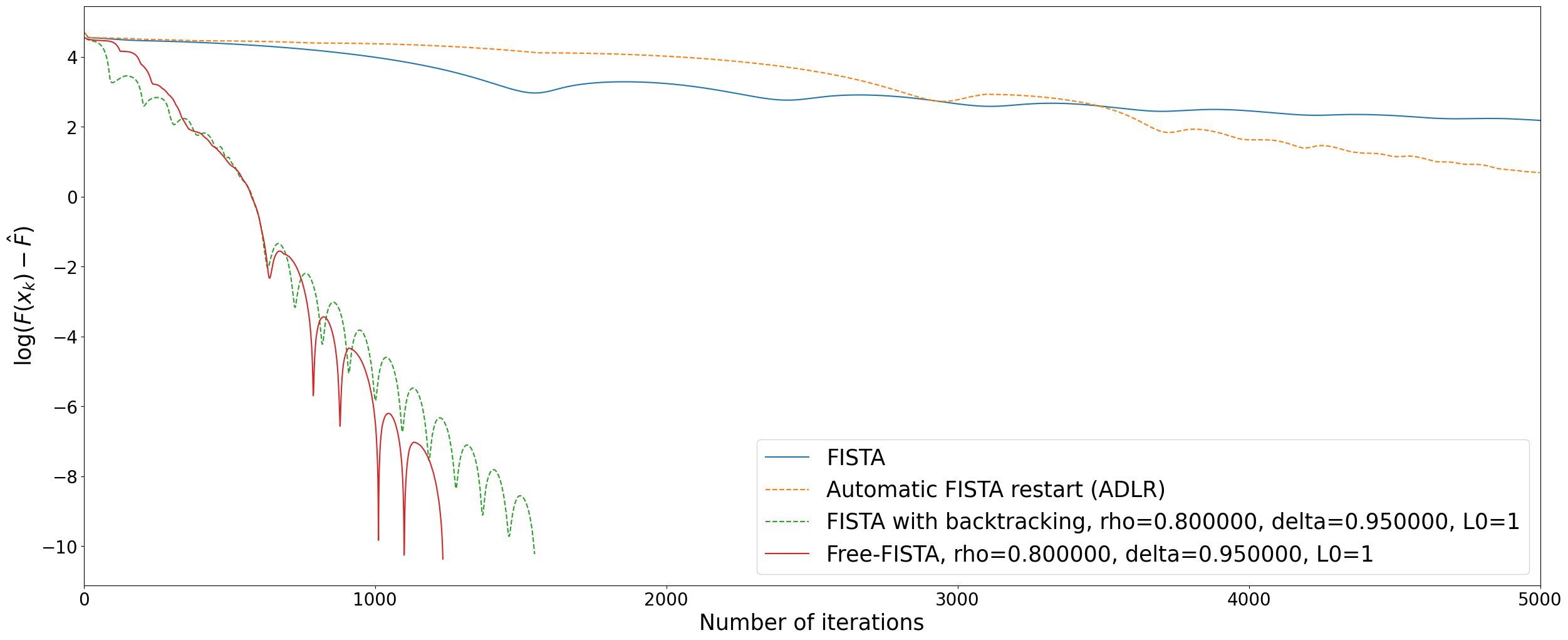
Figure 1: Convergence rates w.r.t. the number of total iterations (backtracking iterations are not taken in account) for problem (4.1).

In Figure 1 the convergence rates of each algorithm are compared w.r.t. the total number of iterations without taking into account the inner iterations required by the backtracking loops. We observe that the use of the adaptive backtracking accelerates both FISTA and FISTA restart. The improved efficiency provided by the combination of restarting and backtracking strategies is highlighted since Free-FISTA is the fastest method. Note, however, that an exhaustive information on the efficiency of each method can not directly be deduced by this plot as the computational burdens required by the use of the inner backtracking routines are not reported. We thus complement our considerations with Figure 2 which allows us to compare the methods w.r.t. the computation time. One can observe that the additional computations required by the backtracking strategy do not prevent the corresponding schemes from being faster.

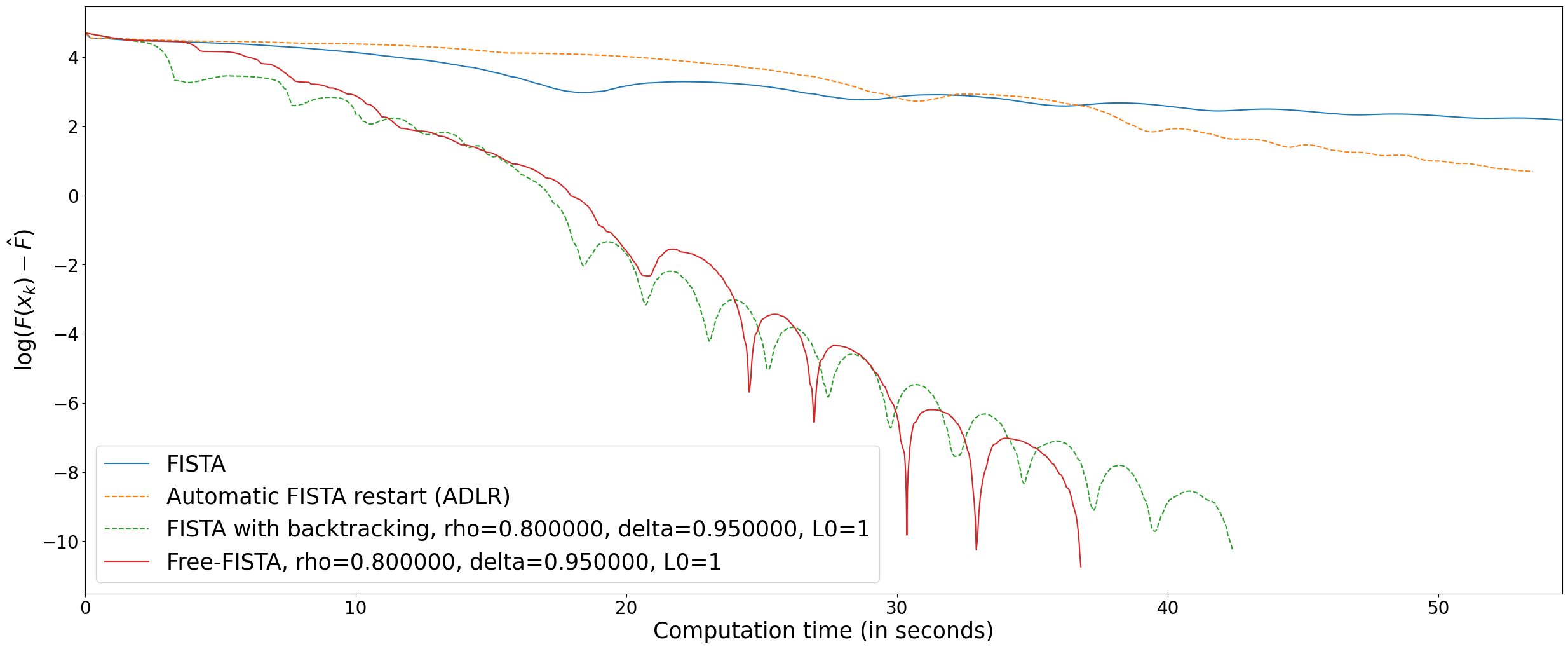
Figure 2: Convergence rates w.r.t. CPU times for problem (4.1).

Figure 3 shows the convergence rate of Free-FISTA w.r.t. the computation time for several parameter choices. We take $\rho=0.8$, $\delta\in\{0.95,0.995\}$ and $L_{0}\in\{1,\hat{L}\}$ where $\hat{L}$ is the upper estimation of the Lipschitz constant of $\nabla f$ given in (4.2) and $1$ is an arbitrary value. This graph shows that Free-FISTA is not highly sensitive to parameter variations in this example. Note that the choice $\delta=0.95$ seems to perform better than $\delta=0.995$. Indeed, as the Lipschitz constant of $\nabla f$ in this problem is poorly estimated, taking a small $\delta$ allows the scheme to explore different choices more efficiently. The value of $L_{0}$ has a small influence on the overall efficiency of the scheme.

Figure 4 gives an overview of the estimations of the Lipschitz constant w.r.t. to FISTA iterations for each parameter choice. We can see that the theoretical upper bound $\hat{L}\geqslant 9\cdot 10^{5}$ is significantly large compared to the estimations computed by Free-FISTA for any set of parameters (the last estimates are approximately equal to $3000$). This explains the substantial performance gap between schemes involving a constant stepsize and backtracking methods (see Figure 1) as a lower Lipschitz constant allows larger stepsizes. In addition, Figure 4 shows that a lower value of $\delta$ encourages larger variations of estimates of $L$ per FISTA iteration, allowing for greater flexibilty.

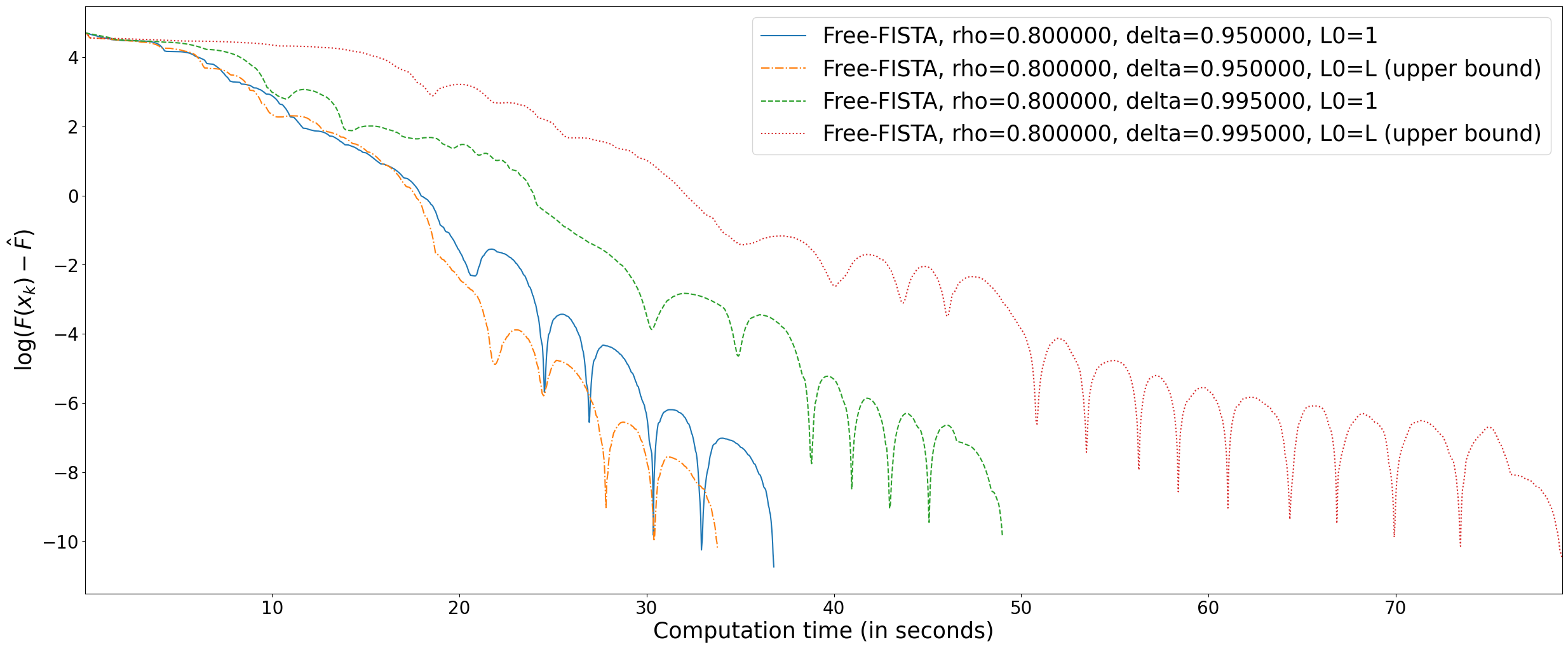
Figure 3: Convergence rates of Free-FISTA for several choices of parameters $\rho$, $\delta$ and $L_{0}$ w.r.t. CPU time for problem (4.1).

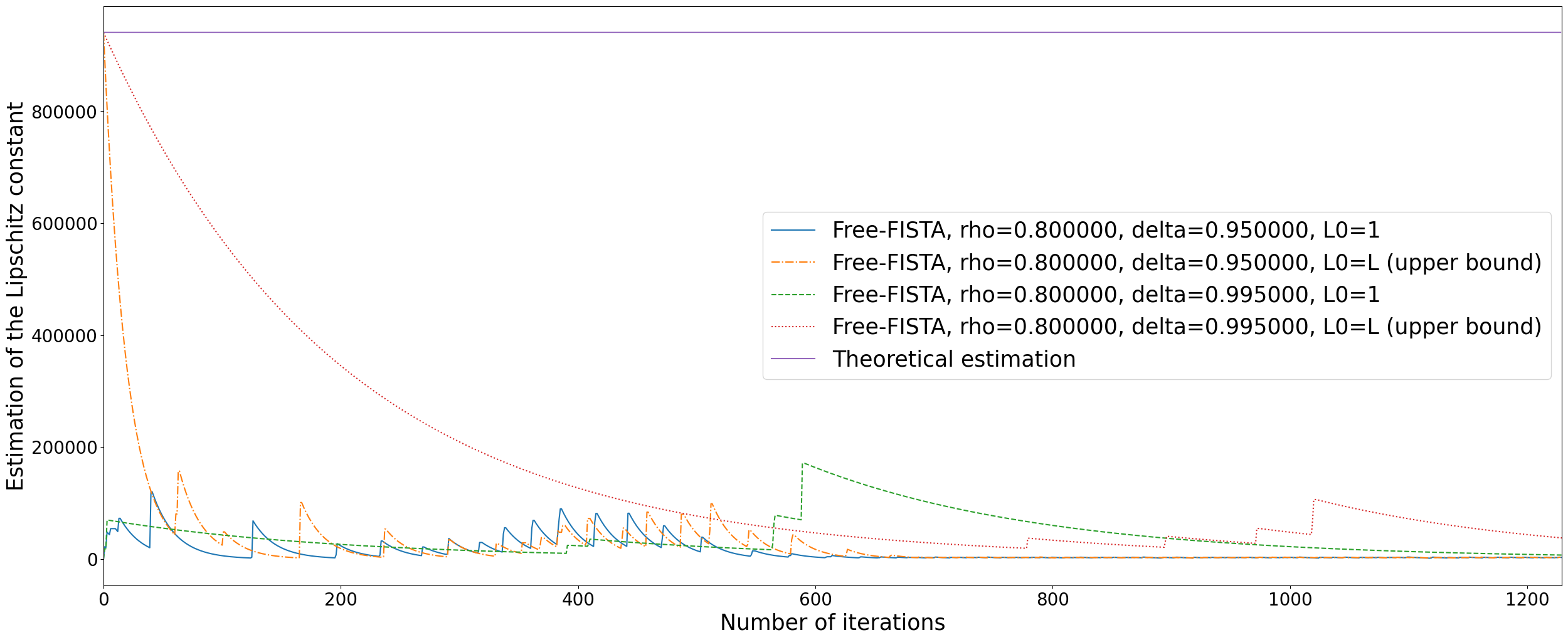
Figure 4: Estimation of the Lipschitz constant of $\nabla f$ according to the number of FISTA iterations for problem (4.1).

In Figure 5, we compare the differences observed between choosing a lower or an upper estimation $L_{0}$ of the Lipschitz constant $L$. Setting $L_{0}$ as a lower estimate forces the backtracking routine to compute a significant number of backtracking iterations before finding an estimate $\tilde{L}$ such that the stepsize $\frac{1}{\tilde{L}}$ is admissible. Once this is done, this estimation is generally tight and the number of backtracking iterations decreases critically. By taking $L_{0}$ as an upper estimate, we observe that the total number of backtracking iterations is smaller, but the estimation of $L$ stays poor for several Free-FISTA iterations (see Figure 4). Both approaches are equally efficient for this example because the high cost of the backtracking routines in the first case is compensated by the small stepsizes in the first FISTA iterations of the second case.

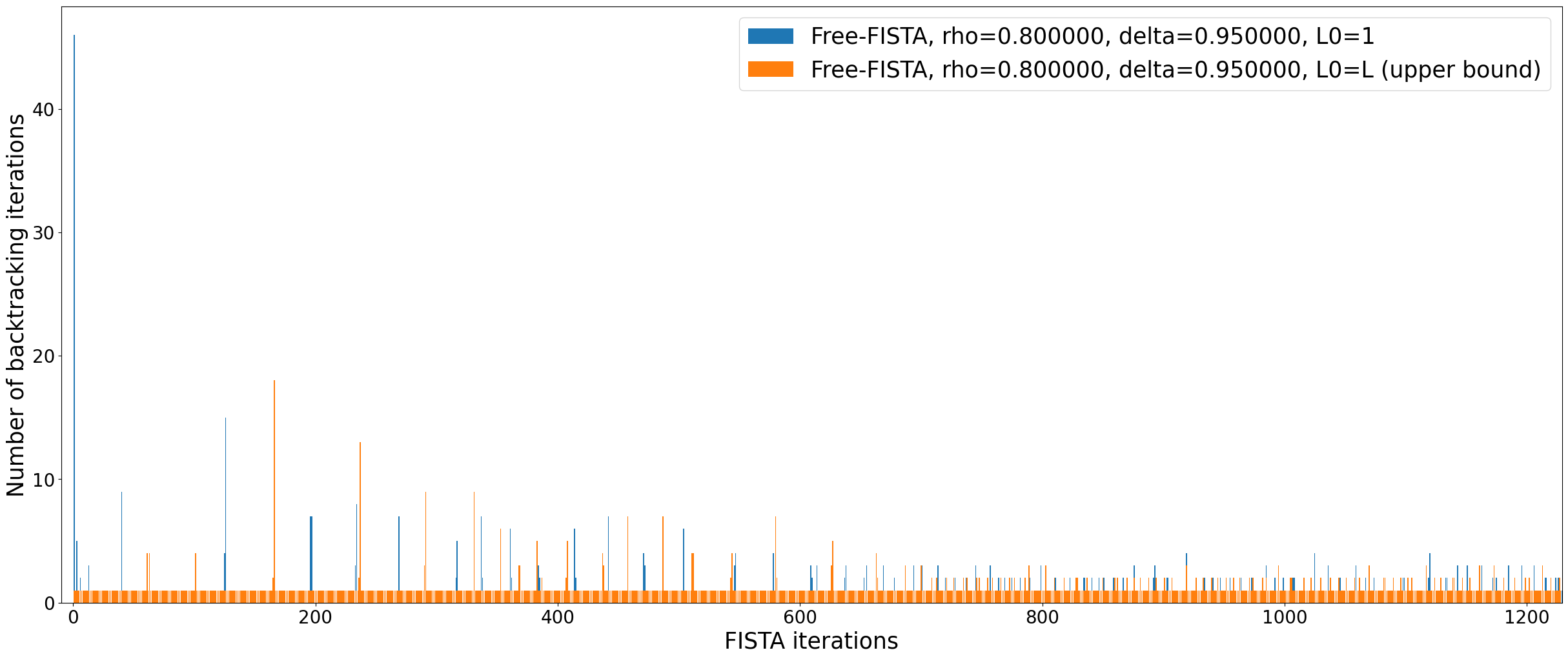
Figure 5: Number of backtracking calls per total FISTA iterations for problem (4.1).

We now follow the experiments provided in [20] and consider the dataset dorothea ($n=100000$ and $m=800$) with $\lambda_{1}=10$ and $\lambda_{2}=\frac{\lambda_{1}\|A^{T}b\|^{2}}{80\|A^{T}b\|_{\infty}n}=0.9097$. Table 1 compares the efficiency of the backtracking and restarting strategies for this example evaluated in terms of the CPU time required to satisfy the stopping condition with $\varepsilon=10^{-5}$. One can observe that methods involving adaptive backtracking are significantly faster. Algorithm 3 is the most efficient algorithms, being, in addition, fully automatic. Some sensitivity to parameters $\rho$ and $\delta$ is observed, which, however, does not seem to significantly impact the overall computational gains.

Algorithm	$\rho$	$\delta$	Time (s)
FISTA	-	-	$28594$
FISTA restart	-	-	$12825$
FISTA_adaBT	$0.85$	$0.95$	$3292$
	$0.8$	$0.95$	$2348$
Free-FISTA	$0.85$	$0.95$	$1173$
	$0.8$	$0.95$	$\mathbf{989}$

Table 1: CPU times (mean over 5 runs) of different algorithms solving (4.1) for the dataset dorothea ($n=10^{6}$ and $m=800$), $\lambda_{1}=10$, $\lambda_{2}=0.9097$ and $\varepsilon=10^{-5}$.

4.2 Image inpainting

We now consider the problem of retrieving an image $\hat{x}\in\mathbb{R}^{N}$ from incomplete measurements $y=M\hat{x}$ where $M\in\mathbb{R}^{N\times N}$ is a masking operator. We consider the regularized approach:

$$\operatorname*{arg\,min}\limits_{x}\leavevmode\nobreak\ F(x):=f(x)+h(x)=\frac{1}{2}\|Mx-y\|^{2}+\lambda\|Tx\|_{1},$$ (4.3)

where $T\in\mathbb{R}^{N\times N}$ is an orthogonal transformation ensuring that $T\hat{x}$ is sparse. For this example we consider $\hat{x}$ to be piece-wise smooth, so that $T$ can be chosen as an orthogonal wavelet transform.

Figure 6: Data for problem (4.3): the damaged image $y$ (left) and an inpainted result (right).

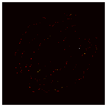
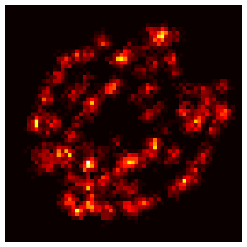
Figure 7: Data for problem (4.5): ground-truth SMLM ISBI13 frame (left), and low-resolution data (right).

The function $F$ satisfies the growth condition $\mathcal{G}^{2}_{\mu}$ for some $\mu>0$ which is not easily computable. In this case, it is trivial to show that an estimate of the Lipschitz constant of $\nabla f$ is $L=1$. Therefore, applying a backtracking strategy may seem superfluous as it involves additional computations. Nonetheless, we apply the methods previously introduced to test their performance with/without restarting. These tests are done on a picture with a resolution of $225\times 225$ pixels, considering the wavelet Daubechies 4 and $\lambda=2$.

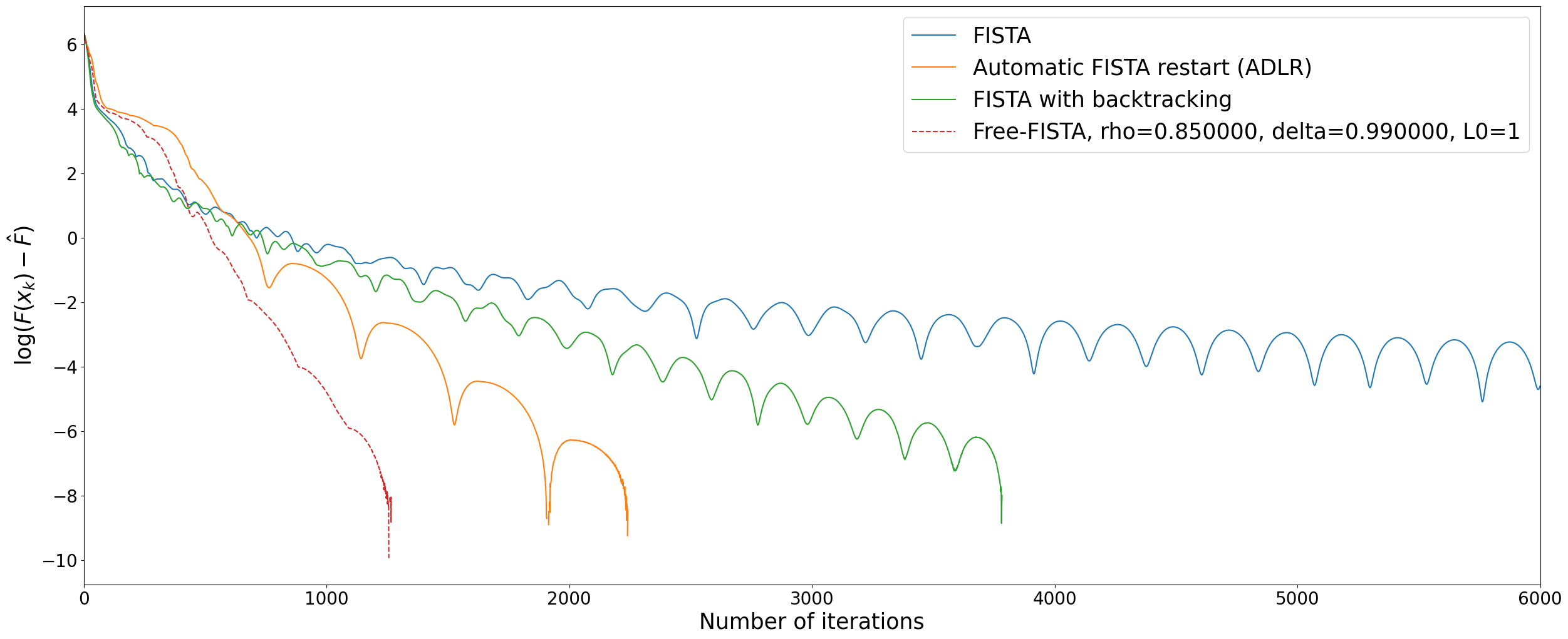
Figure 8: Convergence rates in function values VS. total number of FISTA iterations (backtracking iterations are not taken in account) for problem (4.3).

Figure 8 shows that the backtracking procedure slightly improves the convergence of plain FISTA and FISTA restart w.r.t. the total number of FISTA iterations. Observe that the benefits of backtracking are not as significant as in the previous example since the estimate of the Lipschitz constant $L=1$ is here accurate. In Figure 9 we observe that the additional backtracking loops do not affect the efficiency of the schemes in terms of CPU time. In this example, evaluating $f$ is indeed not expensive which explains their low computational costs.

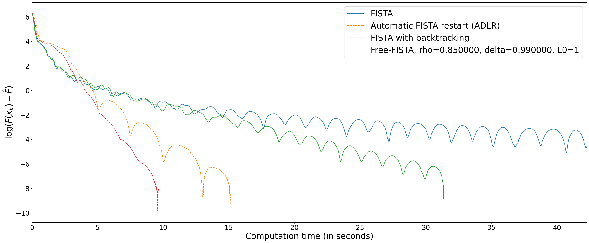
Figure 9: Convergence rates in function values w.r.t the CPU time for problem (4.3).

In Figure 10 we compare the performance of Free-FISTA for different values of $\delta$ and in comparison with ADLR. We observe that $\delta$ should be taken rather large in this case. Contrary to the previous example, if $\delta$ is small ($\delta=0.95$), Free-FISTA performs many unnecessary backtracking iterations to compensate for the over-estimation of the step-sizes, which results in longer CPU times. This can be observed in Figure 11 and Figure 12. By taking $\delta=0.99$, a more gentle estimation with less variability of $L$ is observed over time, with fewer backtracking iterations per FISTA iteration.

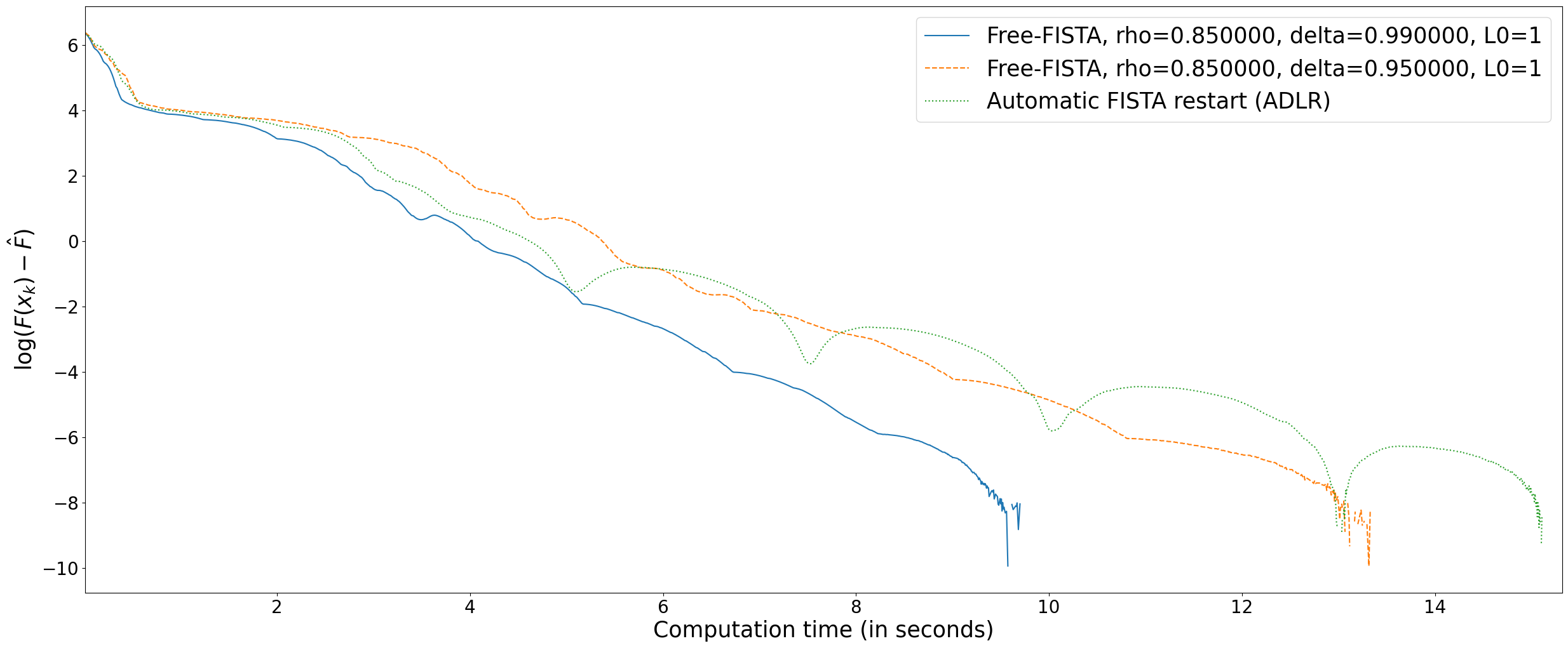
Figure 10: Convergence rates in function valuesw.r.t the CPU time for problem (4.3).

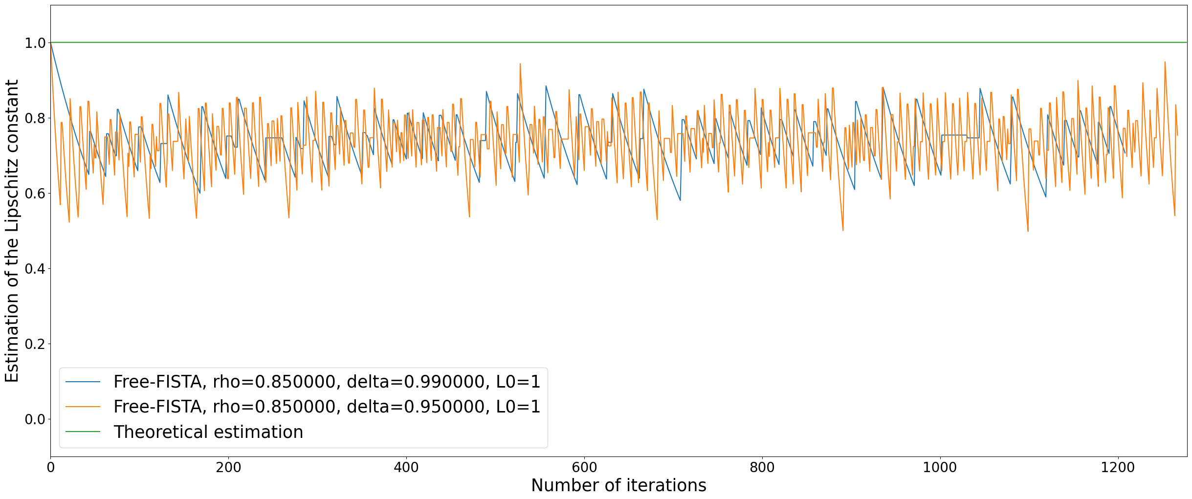
Figure 11: Estimation of the Lipschitz constant of $\nabla f$ according to the number of FISTA iterations for problem (4.3).

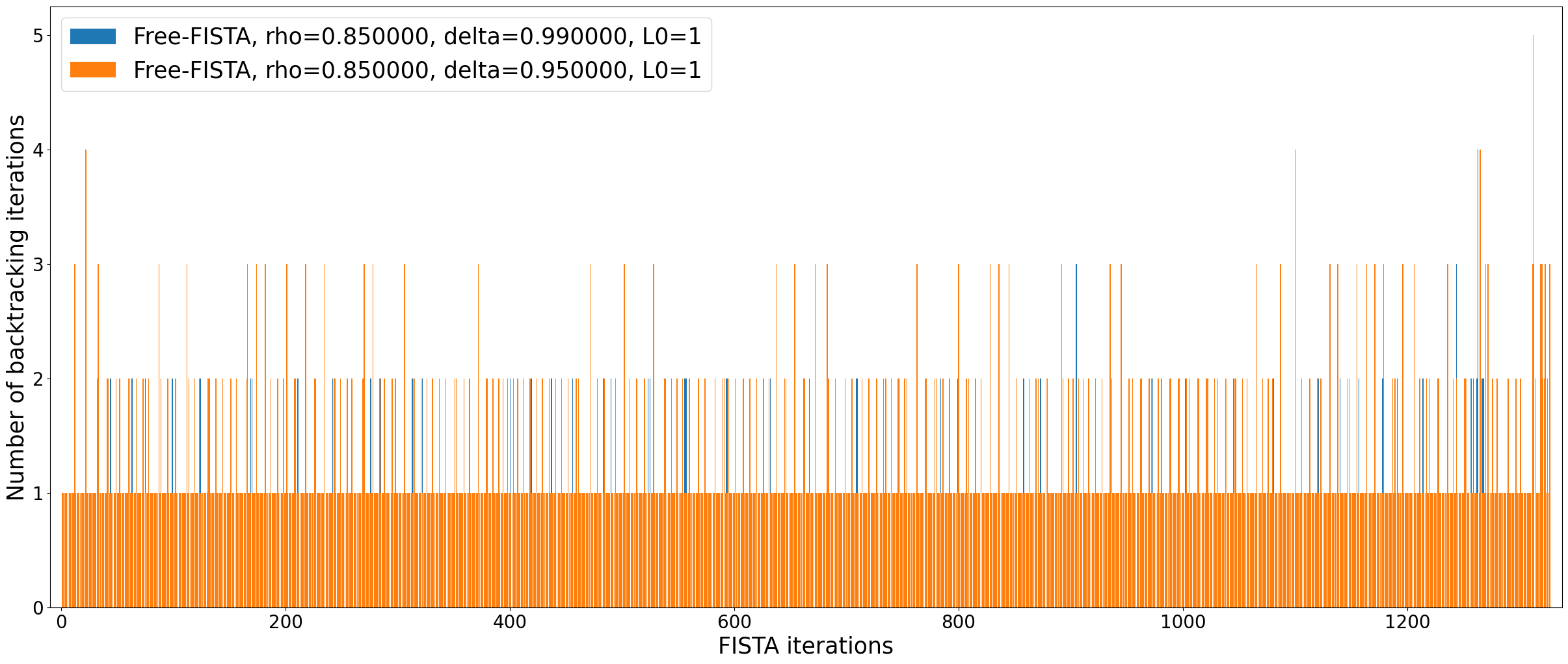
Figure 12: Number of backtracking calls per total FISTA iterations for problem (4.3).

4.3 Poisson image super-resolution with $\ell^{1}$ regularization

As a last example, we consider the image super-resolution problem for images corrupted by Poisson noise, a problem encountered, for instance, in fluorescence microscopy applications[27, 39]. Given a blurred and noisy image $z\in\mathbb{R}_{+}^{m}$, the problem consists in retrieving a sparse and non-negative image $x\in\mathbb{R}_{+}^{n}$ from $z=\mathcal{P}(MHx+b)\in\mathbb{R}^{m}$ with $m=q^{2}n$, $q>1$, where $M\in\mathbb{R}^{m\times n}$ is a $q$-down-sampling operator of factor, $H\in\mathbb{R}^{n\times n}$ is a convolution operator computed for a given point spread function (PSF), $b=\bar{b}e_{m}\in\mathbb{R}^{m}_{>0}$ is a positive constant background term and $\mathcal{P}(w)$ denotes a realization of a Poisson-distributed $m$-dimensional random vector with parameter $w\in\mathbb{R}^{m}_{+}$. To model the presence of Poisson noise in the data, we consider the generalized Kullback-Leibler divergence functional [12] defined by:

$$f(x)=KL(MHx+b;z):=\sum_{i=1}^{m}\left(z_{i}\log\frac{z_{i}}{(MHx)_{i}+\bar{b}}+(MHx)_{i}+\bar{b}-z_{i}\right),$$ (4.4)

and where the convention $0\log 0=0$ is adopted. We enforce sparsity by means of a $\ell^{1}$ penalty and impose non-negativity of the solution using the indicator function $\iota_{\geq 0}(\cdot)$ of the non-negative orthant, so as to consider:

$$\min_{x\in\mathbb{R}^{n}}\leavevmode\nobreak\ F(x):=KL(MHx+b,z)+\lambda\|x\|_{1}+i_{\geq 0}(x).$$ (4.5)

We can compute $\nabla f(x)=(MH)^{T}e_{m}-(MH)^{T}\left(\frac{z}{MHx+b}\right).$ Following [26, 39], we have that $\nabla f$ is Lipschitz continuous on $\left\{x:x\geq 0\right\}$ and its Lipschitz constant $L$ can be overestimated by:

$$L=\frac{\max z_{i}}{\bar{b}^{2}}\max((MH)^{T}e_{m})\max(MHe_{n}).$$ (4.6)

The theoretic estimation of $L$ in (4.6) may be significantly large in particular, when $\bar{b}\ll 1$. Furthermore, as showed in [16], the Kullback-Leibler functional (4.4) is (locally) $2$-conditioned, hence $F$ satisfies $\mathcal{G}^{2}_{\mu}$ for some unknown $\mu>0$. The use of the Free-FISTA Algorithm 3 thus seems appropriate. Results are showed in Figure 13. For this problem, a clear advantage in the use of Free-FISTA in comparison with FISTA with adaptive backtracking cannot be observed. We observe that FISTA with adaptive backtracking is indeed faster in terms of iterations and consequently in terms of complexity (Free-FISTA requires additional computations being based on restarts). We argue that the inefficiency of the restarting strategy can be explained here by the geometry of $F$ in (4.5). The lack of any oscillatory behavior of FISTA endowed with adaptive backtracking suggests indeed that the function $F$ is flat, or, in other words, that $\mu$ is significantly small. Since restarting methods aim to handle the excess of inertia and oscillations, it appears not pertinent to apply such a method in this context.

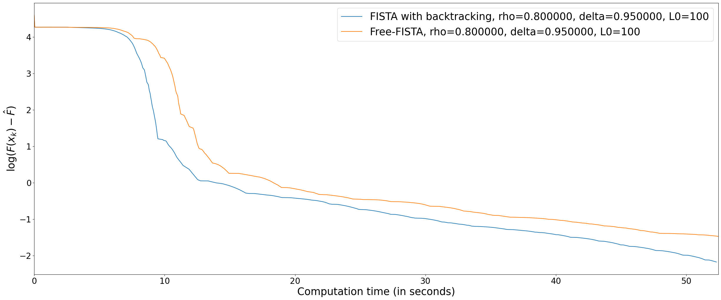
Figure 13: Convergence rates in function values VS. CPU time for problem (4.5).

Appendix A Proofs of the main results

A.1 Proof of Proposition 1

(i) As $F$ satisfies $\mathcal{H}_{L}$ for some $L>0$, Theorem 1 combined with (3.8) states that the sequence $(x_{k})_{k=1,\dots,n}$ provided by Algorithm 1 satisfies for all $k=1,\ldots,n$

$$F(x_{k+1})-F^{*}\leq\frac{2L}{\rho(k+1)^{2}}\|x_{0}-x^{*}\|^{2},$$

for all $x^{*}\in X^{*}$, whence

$$F(x_{k+1})-F^{*}\leqslant\frac{2L}{\rho(k+1)^{2}}\leavevmode\nobreak\ d(x_{0},X^{*})^{2}.$$ (A.1)

Since $F$ further satisfies $\mathcal{G}^{2}_{\mu}$ (2.2), we deduce (3.9) by combining (2.2) and (A.1).

(ii) At each iteration $k\geq 0$ of Algorithm 1, the following condition is satisfied:

$$D_{f}(x_{k+1},y_{k+1})\leqslant\frac{\|x_{k+1}-y_{k+1}\|^{2}}{2\tau_{k+1}}.$$

As a consequence, the descent condition (3.1) becomes:

$$F(x_{k+1})+\frac{\|x_{k+1}-x_{k}\|^{2}}{2\tau^{k+1}}\leqslant F(x_{k})+\frac{\|y_{k+1}-x_{k}\|^{2}}{2\tau_{k+1}}$$

$$\leqslant F(x_{k})+\frac{(t_{k}-1)^{2}}{t_{k+1}^{2}}\frac{\|x_{k}-x_{k-1}\|^{2}}{2\tau_{k+1}}\leqslant F(x_{k})+\frac{(t_{k}-1)^{2}}{t_{k+1}^{2}}\frac{\tau_{k}}{\tau_{k+1}}\frac{\|x_{k}-x_{k-1}\|^{2}}{2\tau_{k}}.$$ (A.2)

By definition, there holds $\tau_{k+1}t_{k+1}(t_{k+1}-1)=\tau_{k}t_{k}^{2}$. Hence:

$$\frac{(t_{k}-1)^{2}}{t_{k+1}^{2}}\frac{\tau_{k}}{\tau_{k+1}}=\frac{(t_{k}-1)^{2}t_{k+1}(t_{k+1}-1)}{t_{k}^{2}t_{k+1}^{2}}\leqslant 1,$$

hence, from (A.2) we get:

$$F(x_{k+1})+\frac{\|x_{k+1}-x_{k}\|^{2}}{2\tau_{k+1}}\leqslant F(x_{k})+\frac{\|x_{k}-x_{k-1}\|^{2}}{2\tau_{k}}$$

for all $k\geq 0$, whence we deduce (3.10).

A.2 Proof of Equation 3.15

Let $(\kappa_{j})_{j\geqslant 2}$ be the sequence defined by

$$\forall j\geqslant 2,\quad\kappa_{j}:=\min\limits_{\underset{i<j}{i\in\mathbb{N}^{*}}}\leavevmode\nobreak\ \frac{4}{\rho(n_{i-1}+1)^{2}}\frac{F(r_{i-1})-F(r_{j})}{F(r_{i})-F(r_{j})}.$$

We prove in this section that $(\kappa_{j})_{j\geqslant 2}$ is non increasing and bounded from below by the true inverse of the conditioning of the considered optimization problem.

First of all, according to Proposition 1, remember that we have (3.13) i.e.

$$\forall i\in\mathbb{N}^{*},\quad\kappa\leqslant\frac{4}{\rho(n_{i-1}+1)^{2}}\frac{F(r_{i-1})-F^{*}}{F(r_{i})-F^{*}}.$$

Since the application $u\mapsto\frac{F(r_{i-1})-u}{F(r_{i})-u}$ is non decreasing on $[F^{*},F(r_{i})]$ (since $F(r_{i})\leqslant F(r_{i-1})$), we deduce that for all $i\in\mathbb{N}^{*}$,

$$\forall i<j,\quad\kappa\leqslant\frac{4}{\rho(n_{i-1}+1)^{2}}\frac{F(r_{i-1})-F(r_{j})}{F(r_{i})-F(r_{j})}.$$

Hence, for a given $j\in\mathbb{N}^{*}$ and taking the infimum over the indexes $i\in\mathbb{N}^{*}$ such that $i<j$, we get: $\kappa\leqslant\kappa_{j}$. To complete the proof, we have that for all $j\geq 2$:

$$\small{\kappa_{j+1}=\min\limits_{\underset{i<j+1}{i\in\mathbb{N}^{*}}}\leavevmode\nobreak\ \frac{4}{\rho(n_{i-1}+1)^{2}}\frac{F(r_{i-1})-F(r_{j+1})}{F(r_{i})-F(r_{j+1})}\leqslant\min\limits_{\underset{i<j}{i\in\mathbb{N}^{*}}}\leavevmode\nobreak\ \frac{4}{\rho(n_{i-1}+1)^{2}}\frac{F(r_{i-1})-F(r_{j+1})}{F(r_{i})-F(r_{j+1})}}$$

by simply observing that in (A.2) the minimum is taken over a larger set. By now applying (3.10) at the $j+1$ restart iteration we have that $F(r_{j+1})\leqslant F(r_{j})$. As a consequence the function defined by $y\mapsto\frac{F(r_{i-1})-y}{F(r_{i})-y}$ is an increasing homographic function which implies that for all $j\geq 2$:

$$\small{\kappa_{j+1}\leqslant\min\limits_{\underset{i<j}{i\in\mathbb{N}^{*}}}\leavevmode\nobreak\ \frac{4}{\rho(n_{i-1}+1)^{2}}\frac{F(r_{i-1})-F(r_{j+1})}{F(r_{i})-F(r_{j+1})}\leqslant\min\limits_{\underset{i<j}{i\in\mathbb{N}^{*}}}\leavevmode\nobreak\ \frac{4}{\rho(n_{i-1}+1)^{2}}\frac{F(r_{i-1})-F(r_{j})}{F(r_{i})-F(r_{j})}=\kappa_{j}.}$$

A.3 Proof of Lemma 2

Suppose that $F$ satisfies $\mathcal{H}_{L}$ and $\mathcal{G}^{2}_{\mu}$ for some $L>0$ and $\mu>0$. Then, by Lemma 1

$$\forall x\in\mathbb{R}^{N},\quad F(x)-F^{*}\leqslant\frac{2}{\mu}d(0,\partial F(x))^{2}.$$

Let now $x\in\mathbb{R}^{N}$ and $\tau>0$. By definition (2.1), $x^{+}=T_{\tau}x$ is the unique minimizer of the function defined by $z\mapsto h(z)+\frac{1}{2\tau}\|z-x+\tau\nabla f(x)\|^{2}$. Thus, $T_{\tau}x$ satisfies

$$0\in\partial h(T_{\tau}x)+\left\{\frac{1}{\tau}(T_{\tau}x-x)+\nabla f(x)\right\},$$

which entails: $g_{\tau}(x)-\nabla f(x)+\nabla f(T_{\tau}x)\in\partial F(T_{\tau}x)$. By the $L$-Lipschitz continuity of $\nabla f$ we can now deduce

$$\|g_{\tau}(x)-\nabla f(x)+\nabla f(T_{\tau}x)\|\leqslant\|g_{\tau}(x)\|+\|\nabla f(T_{\tau}x)-\nabla f(x)\|$$

$$\leqslant\|g_{\tau}(x)\|+L\|T_{\tau}x-x\|\leqslant(1+L\tau)\|g_{\tau}(x)\|.$$

By combining all these inequalities we conclude that

$$\small{F(T_{\tau}x)-F^{*}\leqslant\frac{2}{\mu}d(0,\partial F(T_{\tau}x))^{2}\leqslant\frac{2}{\mu}\|g_{\tau}(x)-\nabla f(x)+\nabla f(T_{\tau}x)\|^{2}\leqslant\frac{2(1+L\tau)^{2}}{\mu}\|g_{\tau}(x)\|^{2}.}$$

A.4 Sketch of the proof of Theorem 2

Since the proof is rather technical, we split it into the following two parts:

1. We show that there is at least one doubling step every $T$ iterations for a suitable $T$. In particular:

   1. We suppose that there is no doubling step from $j=s+1$ to $j=s+T$ for $s\geq 1$.

   2. We show a geometrical decrease of $(F(r_{j-1})-F(r_{j}))_{j\in\llbracket s+1,s+T\rrbracket}$ where the factor represents the gain of the $j$-th execution of Algorithm 1.

   3. We state and apply Lemma 5 (whose proof is given in Subsection A.7) to show that there exists an upper bound for $\|g_{1/{L}_{j-1}^{+}}(r_{j-1})\|$ depending on $F(r_{j-1})-F(r_{j})$ for all $j\in\llbracket s+1,s+T\rrbracket$.

   4. We show that the geometrical decrease in (b) entails that the exit condition $\|g_{1/{L}_{j-1}^{+}}(r_{j-1})\|\leq\varepsilon$ is satisfied for $j=s+T$.

2. We use 1. to show that the total number of restarting iterations $\sum_{i=0}^{j}n_{i}$ is necessarily bounded by $2Tn_{j}$. The conclusion of Theorem 2 thus comes from Lemma 4 providing an upper bound of $n_{j}$.

A.5 Proof of Theorem 2

Let $C>\frac{4}{\sqrt{\rho}}$ and $\varepsilon>0$. We first define

$$T:=1+\left\lceil\frac{\log\left(1+\frac{16}{C^{2}\rho-16}\frac{2L(F(r_{0})-F^{*})}{\rho\varepsilon^{2}}\right)}{\log\left(\frac{C^{2}\rho}{4}-1\right)}\right\rceil.$$

We claim that a doubling step is performed at least every $T$ iterations.
For $s\geqslant 1$, assume that there is no doubling step for $T-1$ iterations from $j=s+1$ to $j=s+T$. This means:

$$\forall j\in\llbracket s+1,s+T\rrbracket,\quad n_{j-1}>C\sqrt{\frac{1}{\kappa_{j}}},$$ (A.3)

whence:

$$\forall j\in\llbracket s,s+T\rrbracket,\quad n_{j}=n_{s},$$ (A.4)

where the case $j=s$ trivially holds. We deduce that $\forall j\in\llbracket s+2,s+T\rrbracket$:

$${\kappa}_{j} =\min\limits_{\underset{i<j}{i\in\mathbb{N}^{*}}}\frac{4}{\rho(n_{i-1}+1)^{2}}\frac{F(r_{i-1})-F(r_{j})}{F(r_{i})-F(r_{j})}\leqslant\min\limits_{\underset{s<i<j}{i\in\mathbb{N}^{*}}}\frac{4}{\rho(n_{i-1}+1)^{2}}\frac{F(r_{i-1})-F(r_{j})}{F(r_{i})-F(r_{j})}$$

$$\leqslant\min\limits_{\underset{s<i<j}{i\in\mathbb{N}^{*}}}\frac{4}{\rho{n_{i-1}}^{2}}\frac{F(r_{i-1})-F(r_{j})}{F(r_{i})-F(r_{j})}\leqslant\min\limits_{\underset{s<i<j}{i\in\mathbb{N}^{*}}}\frac{4}{\rho{n_{s}}^{2}}\frac{F(r_{i-1})-F(r_{j})}{F(r_{i})-F(r_{j})}$$

$$\leqslant\frac{4}{\rho{n_{s}}^{2}}\min\limits_{\underset{s<i<j}{i\in\mathbb{N}^{*}}}\frac{F(r_{i-1})-F(r_{j})}{F(r_{i})-F(r_{j})},$$

due to (A.4). Using (3.10), we deduce that:

$$\forall j\in\llbracket s+2,s+T\rrbracket,\quad{\kappa}_{j}\leqslant\frac{4}{\rho{n_{s}}^{2}}\frac{F(r_{j-2})-F(r_{j})}{F(r_{j-1})-F(r_{j})}.$$ (A.5)

Combining now (A.3) with (A.4) and (A.5) we get:

$$n_{s}>C\sqrt{\frac{1}{\frac{4}{\rho{n_{s}}^{2}}\frac{F(r_{j-2})-F(r_{j})}{F(r_{j-1})-F(r_{j})}}}=n_{s}\frac{C\sqrt{\rho}}{2}\sqrt{\frac{F(r_{j-1})-F(r_{j})}{F(r_{j-2})-F(r_{j})}}$$

which leads to

$$F(r_{j-2})-F(r_{j})>\frac{C^{2}\rho}{4}(F(r_{j-1})-F(r_{j})),$$

which further entails

$$F(r_{j-2})-F(r_{j-1})>\left(\frac{C^{2}\rho}{4}-1\right)(F(r_{j-1})-F(r_{j})).$$

Since $C>\frac{4}{\sqrt{\rho}}>\frac{2}{\sqrt{\rho}}$ we now get the following geometric functional decrease.

$$F(r_{j-1})-F(r_{j})<\frac{4}{C^{2}\rho-4}(F(r_{j-2})-F(r_{j-1})).$$ (A.6)

We now consider the case $j=s+1$:

$$\kappa_{s+1} =\min\limits_{\underset{i<s+1}{i\in\mathbb{N}^{*}}}\frac{4}{\rho(n_{i-1}+1)^{2}}\frac{F(r_{i-1})-F(r_{s+1})}{F(r_{i})-F(r_{s+1})}\leqslant\frac{4}{\rho(n_{s-1}+1)^{2}}\frac{F(r_{s-1})-F(r_{s+1})}{F(r_{s})-F(r_{s+1})}$$

$$\leqslant\frac{4}{\rho(\frac{n_{s}}{2}+1)^{2}}\frac{F(r_{s-1})-F(r_{s+1})}{F(r_{s})-F(r_{s+1})}\leqslant\frac{16}{\rho{n_{s}}^{2}}\frac{F(r_{s-1})-F(r_{s+1})}{F(r_{s})-F(r_{s+1})},$$

since $n_{s}\leqslant 2n_{s-1}$. By reapplying $C>\frac{4}{\sqrt{\rho}}$, similar computations show that

$$F(r_{s})-F(r_{s+1})<\frac{16}{C^{2}\rho-16}(F(r_{s-1})-F(r_{s})).$$ (A.7)

To carry on with the proof, we now state Lemma 5 which links the composite gradient mapping $g$ to the function $F$. The proof is reported in Section A.7:

Lemma 5

Let $F$ satisfy the assumption $\mathcal{H}_{L}$ for some $L>0$. Then the sequence $(r_{j})_{j\in\mathbb{N}}$ provided by Algorithm 3 satisfies

$$\forall j\geqslant 1,\quad\frac{\rho}{2L}\|g_{1/{L}_{j}^{+}}(r_{j})\|^{2}\leqslant F(r_{j})-F(r_{j+1}),$$

where ${L}_{j}^{+}$ is an estimate of $L$ provided by Algorithm 2.

By Lemma 5 and recalling inequalities (A.6) and (A.7), we can thus obtain the following sequence of inequalities

$$\frac{\rho}{2L}\|g_{1/{L}_{s+T-1}^{+}}(r_{s+T-1})\|^{2}\leqslant F(r_{s+T-1})-F(r_{s+T})$$

$$\leqslant\frac{4}{C^{2}\rho-4}(F(r_{s+T-2})-F(r_{s+T-1}))$$

$$\leqslant\left(\frac{4}{C^{2}\rho-4}\right)^{T-1}\left(\frac{16}{C^{2}\rho-16}\right)(F(r_{s-1})-F(r_{s}))$$

$$\leqslant\left(\frac{4}{C^{2}\rho-4}\right)^{T-1}\left(\frac{16}{C^{2}\rho-16}\right)(F(r_{0})-F^{*})$$

$$\leqslant\left(\frac{4}{C^{2}\rho-4}\right)^{\left\lceil\frac{\log\left(1+\frac{16}{C^{2}\rho-16}\frac{2L(F(r_{0})-F^{*})}{\rho\varepsilon^{2}}\right)}{\log\left(\frac{C^{2}\rho}{4}-1\right)}\right\rceil}\left(\frac{16}{C^{2}\rho-16}\right)(F(r_{0})-F^{*})$$

$$\leqslant\left(\frac{4}{C^{2}\rho-4}\right)^{\frac{\log\left(1+\frac{16}{C^{2}\rho-16}\frac{2L(F(r_{0})-F^{*})}{\rho\varepsilon^{2}}\right)}{\log\left(\frac{C^{2}\rho}{4}-1\right)}}\left(\frac{16}{C^{2}\rho-16}\right)(F(r_{0})-F^{*})$$

$$\leqslant\frac{1}{1+\frac{16}{C^{2}\rho-16}\frac{2L(F(r_{0})-F^{*})}{\rho\varepsilon^{2}}}\left(\frac{16}{C^{2}\rho-16}\right)(F(r_{0})-F^{*})\leqslant\frac{\rho\varepsilon^{2}}{2L}.$$

As a consequence, if there are $T$ consecutive restarts without any doubling of the number of iterations, then the exit condition $\|g_{1/{L}_{j}^{+}}(r_{j})\|\leqslant\varepsilon$ is eventually satisfied. This means that there exists a doubling step at least every $T$ steps and that for all $s\geqslant 1$ there exists $j\in\llbracket s+1,s+T\rrbracket$ such that

$$n_{j-1}<C\sqrt{\frac{1}{\kappa_{j}}},$$

which implies that $n_{j}=2n_{j-1}$. Now, since $(n_{j})_{j\in\mathbb{N}}$ is an increasing sequence, we get that $n_{s+T}\geqslant n_{j}=2n_{j-1}\geqslant 2n_{s}$, so that

$$n_{s}\leqslant\frac{n_{s+T}}{2},\leavevmode\nobreak\ \quad\forall s\geqslant 1.$$ (A.8)

Let us now rewrite $j$ as $j=m+nT$ where $0\leqslant m<T$ and $n\geqslant 0$. By monotonicity of $(n_{j})_{j\in\mathbb{N}}$ we have

$$\sum_{i=0}^{j}n_{i}=\sum_{i=0}^{m+nT}n_{i}=\sum_{i=0}^{m}n_{i}+\sum_{l=0}^{n-1}\sum_{i=1}^{T}n_{m+i+lT}\leqslant T\sum_{l=0}^{n}n_{m+lT}=T\sum_{l=0}^{n}n_{j-lT}.$$

According to equation (A.8) we have $n_{j-T}\leqslant\frac{n_{j}}{2}$, that is

$$n_{j-lT}\leqslant\left(\frac{1}{2}\right)^{l}n_{j},\quad\forall l\in[\![0,n]\!].$$

We thus obtain the following inequalities

$$\sum_{i=0}^{j}n_{i}\leqslant T\sum_{l=0}^{n}n_{j-lT}\leqslant T\sum_{l=0}^{n}\left(\frac{1}{2}\right)^{l}n_{j}\leqslant T\sum_{l=0}^{\infty}\left(\frac{1}{2}\right)^{l}n_{j}=2Tn_{j}.$$ (A.9)

Combining (A.9) with Lemma 4 we thus finally get the desired result for $j>0$

$$\sum_{i=0}^{j}n_{i} \leqslant 2Tn_{j}\leqslant 4C\sqrt{\frac{L}{\mu}}T\leqslant 4C\sqrt{\frac{L}{\mu}}\left(1+\left\lceil\frac{\log\left(1+\frac{16}{C^{2}\rho-16}\frac{2L(F(r_{0})-F^{*})}{\rho\varepsilon^{2}}\right)}{\log\left(\frac{C^{2}\rho}{4}-1\right)}\right\rceil\right)$$

$$\leqslant\frac{4C}{\log\left(\frac{C^{2}\rho}{4}-1\right)}\sqrt{\frac{L}{\mu}}\left(2\log\left(\frac{C^{2}\rho}{4}-1\right)+\log\left(1+\frac{16}{C^{2}\rho-16}\frac{2L(F(r_{0})-F^{*})}{\rho\varepsilon^{2}}\right)\right).$$

A.6 Proof of Corollary 1

Let $F$ satisfy $\mathcal{H}_{L}$ and $\mathcal{G}^{2}_{\mu}$ for some $L>0$ and $\mu>0$. Let $(r_{j})_{j\in\mathbb{N}}$ and $(n_{j})_{j\in\mathbb{N}}$ be the sequences provided by Algorithm 3 with $C>4/\sqrt{\rho}$, $\varepsilon>0$ and let $L_{min}\in(0,L)$. We consider the case where the exit condition $\|g_{1/{L}_{j}^{+}}(r_{j})\|\leqslant\varepsilon$ is satisfied at first for at least $8C\sqrt{\frac{1}{\kappa}}$ iterations. We define the function $\psi_{\mu}:\mathbb{R}_{+}^{*}\rightarrow\left(8C\sqrt{\frac{1}{\kappa}},+\infty\right)$ by:

$$\psi_{\mu}:\gamma\mapsto\frac{4C}{\log\left(\frac{C^{2}\rho}{4}-1\right)}\sqrt{\frac{L}{\mu}}\left(2\log\left(\frac{C^{2}\rho}{4}-1\right)+\log\left(1+\frac{16}{C^{2}\rho-16}\frac{2L(F(r_{0})-F^{*})}{\rho\gamma}\right)\right).$$

By Theorem 2, the number of iterations required to ensure $\|g_{1/{L}_{j}^{+}}(r_{j})\|\leqslant\varepsilon$ satisfies $\sum_{i=0}^{j}n_{i}\leqslant\psi_{\mu}(\varepsilon^{2})$. As $\psi_{\mu}$ is strictly decreasing and $\sum_{i=0}^{j}n_{i}>8C\sqrt{\frac{L}{\mu}}$, we deduce:

$$\psi_{\mu}^{-1}\left(\sum_{i=0}^{j}n_{i}\right)\geqslant\varepsilon^{2},$$

where $\psi_{\mu}^{-1}$ is the inverse function of $\psi_{\mu}$. By now applying Lemma 2 and since by construction ${L}_{j}^{+}\geqslant L_{min}$, we get:

$$\small{F({r}_{j}^{+})-F^{*}\leqslant\frac{2\left(1+\frac{L}{{L}_{j}^{+}}\right)^{2}}{\mu}\|g_{1/{L}_{j}^{+}}(r_{j})\|^{2}\leqslant\frac{2\left(1+\frac{L}{L_{min}}\right)^{2}}{\mu}\psi_{\mu}^{-1}\left(\sum_{i=0}^{j}n_{i}\right).}$$ (A.10)

Elementary computations show that:

$$\psi_{\mu}^{-1}:n\mapsto\frac{2L}{\rho}\frac{16}{C^{2}\rho-16}\frac{1}{e^{-2\log(\frac{C^{2}\rho}{4}-1)}e^{\frac{\log(\frac{C^{2}\rho}{4}-1)}{4C}\sqrt{\frac{\mu}{L}}n}-1}(F(r_{0})-F^{*}),$$

hence from (A.10), we get:

$$F({r}_{j}^{+})-F^{*}\leqslant\frac{4L\left(1+\frac{L}{L_{min}}\right)^{2}}{\rho\mu}\frac{16}{C^{2}\rho-16}\frac{1}{e^{-2\log(\frac{C^{2}\rho}{4}-1)}e^{\frac{\log(\frac{C^{2}\rho}{4}-1)}{4C}\sqrt{\frac{\mu}{L}}\sum_{i=0}^{j}n_{i}}-1}(F(r_{0})-F^{*})$$

We can thus conclude that

$$F({r}_{j}^{+})-F^{*}=\mathcal{O}\left(e^{-\frac{\log(\frac{C^{2}\rho}{4}-1)}{4C}\sqrt{\kappa}\sum_{i=0}^{j}n_{i}}\right).$$

We can further maximize the function $C\mapsto\frac{\log(\frac{C^{2}\rho}{4}-1)}{4C}$ to obtain the optimal value $\hat{C}\approx 6.38/\sqrt{\rho}$. This choice leads to the desired convergence rate:

$$F({r}_{j}^{+})-F^{*}=\mathcal{O}\left(e^{-\frac{\sqrt{\rho}}{12}\sqrt{\kappa}\sum_{i=0}^{j}n_{i}}\right).$$

To conclude the proof, let now $\left(x_{k,j}\right)_{k\in\llbracket 0,n_{j}\rrbracket}$ and $\left(\tau_{k,j}\right)_{k\in\llbracket 0,n_{j}\rrbracket}$ denote the iterates of Algorithm 1 following the $j$-th restart and the corresponding step-sizes, respectively. Note that in particular we have $x_{0,j}=r_{j-1}^{+}$ and $x_{n_{j},j}=r_{j}$. By applying standard arguments as in the proof of Proposition 1 (see Section A.1) we deduce that for any $j\geqslant 0$ and every $k>0$:

$$F(x_{k,j})+\frac{\|x_{k,j}-x_{k-1,j}\|^{2}}{2\tau_{k,j}}\leqslant F(x_{0,j}).$$

Such inequality thus entails:

$$\|x_{k,j}-x_{k-1,j}\|^{2}\leqslant 2\tau_{k,j}\left(F(r_{j}^{+})-F^{*}\right)\leqslant\frac{2}{L_{min}}\left(F(r_{j}^{+})-F^{*}\right).$$

By applying the first claim of this Corollary on the right hand side of the inequality above, we guarantee the existence of $M>0$ such that for $j$ large enough:

$$\forall k\in\llbracket 1,n_{j}\rrbracket,\quad\|x_{k,j}-x_{k-1,j}\|^{2}\leqslant\frac{2M}{L_{min}}e^{-\frac{\log(\frac{C^{2}\rho}{4}-1)}{4C}\sqrt{\kappa}\sum_{i=0}^{j}n_{i}},$$

which implies that $\sum_{j,k}\|x_{k,j}-x_{k-1,j}\|<+\infty,$ showing that the trajectory of the total number of FISTA iterates has finite length.

A.7 Proof of Lemma 5

Since by definition $({r}_{j}^{+},{L}_{j}^{+})=\text{{FB\_BT}}(r_{j},{L}_{j};\rho)$, for all $j\geqslant 1$ there holds: $D_{f}({r}_{j}^{+},r_{j})\leqslant\frac{{L}_{j}^{+}}{2}\|{r}_{j}^{+}-r_{j}\|^{2},$ with ${r}_{j}^{+}=T_{1/{L}_{j}^{+}}(r_{j})$ which allows us to specialize the descent condition (3.1) as:

$$F({r}_{j}^{+})+\frac{{L}_{j}^{+}}{2}\|{r}_{j}^{+}-x\|^{2}\leqslant F(x)+\frac{{L}_{j}^{+}}{2}\|r_{j}-x\|^{2},$$

for all $x\in\mathbb{R}^{N}$. By choosing $x=r_{j}$ and by definition of $g_{1/{L}_{j}^{+}}$ we get:

$$\frac{1}{2L_{j}^{+}}\|g_{1/L_{j}^{+}}r_{j}\|^{2}\leqslant F(r_{j})-F({r}_{j}^{+}).$$

Since by (3.3), we further deduce $L_{j}^{+}\leqslant\frac{L}{\rho}$,

$$\frac{\rho}{2L}\|g_{1/L_{j}^{+}}(r_{j})\|^{2}\leqslant F(r_{j})-F({r}_{j}^{+}).$$

Inequality (3.10) ensures $F(r_{j+1})\leqslant F({r}_{j}^{+})$ which finally entails.

$$\frac{\rho}{2L}\|g_{1/L_{j}^{+}}(r_{j})\|^{2}\leqslant F(r_{j})-F(r_{j+1}).$$

References

• [1] T. Alamo, P. Krupa, and D. Limon, Gradient based restart FISTA, in 2019 IEEE 58th Conference on Decision and Control (CDC), IEEE, 2019, pp. 3936–3941.
• [2] T. Alamo, P. Krupa, and D. Limon, Restart of accelerated first order methods with linear convergence under a quadratic functional growth condition, IEEE Transactions on Automatic Control, (2022).
• [3] T. Alamo, D. Limon, and P. Krupa, Restart FISTA with global linear convergence, in 2019 18th European Control Conference (ECC), IEEE, 2019, pp. 1969–1974.
• [4] H. Attouch and A. Cabot, Convergence rates of inertial forward-backward algorithms, SIAM Journal on Optimization, 28 (2018), pp. 849–874.
• [5] H. Attouch and J. Peypouquet, The rate of convergence of Nesterov’s accelerated forward-backward method is actually faster than $1/k^{2}$, SIAM Journal on Optimization, 26 (2016), pp. 1824–1834.
• [6] J.-F. Aujol, C. Dossal, and A. Rondepierre, Convergence rates of the Heavy-Ball method under the łojasiewicz property, Mathematical Programming, 198 (2023), pp. 195–254.
• [7] J.-F. Aujol, C. Dossal, and A. Rondepierre, FISTA is an automatic geometrically optimized algorithm for strongly convex functions, Mathematical Programming, (2023).
• [8] J.-F. Aujol, C. H. Dossal, H. Labarrière, and A. Rondepierre, FISTA restart using an automatic estimation of the growth parameter. HAL preprint: https://hal.archives-ouvertes.fr/hal-03153525v3/file/Adaptive_restart.pdf.
• [9] A. Beck, First-Order Methods in Optimization, Society for Industrial and Applied Mathematics, Philadelphia, PA, 2017.
• [10] A. Beck and M. Teboulle, Fast gradient-based algorithms for constrained total variation image denoising and deblurring problems, IEEE transactions on image processing, 18 (2009), pp. 2419–2434.
• [11] A. Beck and M. Teboulle, A fast iterative shrinkage-thresholding algorithm for linear inverse problems, SIAM journal on imaging sciences, 2 (2009), pp. 183–202.
• [12] M. Bertero, P. Boccacci, and V. Ruggiero, Inverse Imaging with Poisson Data, 2053-2563, IOP, 2018.
• [13] J. Bolte, T. P. Nguyen, J. Peypouquet, and B. W. Suter, From error bounds to the complexity of first-order descent methods for convex functions, Mathematical Programming, 165 (2017), pp. 471–507.
• [14] S. Bonettini, S. Rebegoldi, and V. Ruggiero, Inertial variable metric techniques for the inexact forward–backward algorithm, SIAM Journal on Scientific Computing, 40 (2018), pp. A3180–A3210.
• [15] L. Calatroni and A. Chambolle, Backtracking strategies for accelerated descent methods with smooth composite objectives, SIAM journal on optimization, 29 (2019), pp. 1772–1798.
• [16] L. Calatroni, G. Garrigos, L. Rosasco, and S. Villa, Accelerated iterative regularization via dual diagonal descent, SIAM Journal on Optimization, 31 (2021), pp. 754–784.
• [17] A. Chambolle and C. Dossal, On the convergence of the iterates of the “fast iterative shrinkage/thresholding algorithm”, Journal of Optimization theory and Applications, 166 (2015), pp. 968–982.
• [18] A. Chambolle and T. Pock, An introduction to continuous optimization for imaging, Acta Numerica, 25 (2016), pp. 161–319.
• [19] P. L. Combettes and V. R. Wajs, Signal recovery by proximal forward-backward splitting, Multiscale Modeling & Simulation, 4 (2005), pp. 1168–1200.
• [20] O. Fercoq and Z. Qu, Adaptive restart of accelerated gradient methods under local quadratic growth condition, IMA Journal of Numerical Analysis, 39 (2019), pp. 2069–2095.
• [21] Q. Fercoq and Z. Qu, Restarting accelerated gradient methods with a rough strong convexity estimate, (2016). arXiv preprint: https://arxiv.org/pdf/1609.07358.
• [22] M. I. Florea and S. A. Vorobyov, A generalized accelerated composite gradient method: Uniting nesterov’s fast gradient method and fista, IEEE Transactions on Signal Processing, 68 (2020), pp. 3033–3048.
• [23] G. Garrigos, L. Rosasco, and S. Villa, Convergence of the forward-backward algorithm: beyond the worst-case with the help of geometry, Mathematical Programming, 198 (2023), pp. 937–996.
• [24] T. Goldstein, C. Studer, and R. Baraniuk, A field guide to forward-backward splitting with a fasta implementation, 2014, https://arxiv.org/abs/1411.3406.
• [25] C. C. Gonzaga and E. W. Karas, Fine tuning nesterov’s steepest descent algorithm for differentiable convex programming, Mathematical Programming, 138 (2013), pp. 141–166.
• [26] Z. T. Harmany, R. F. Marcia, and R. M. Willett, This is SPIRAL-TAP: Sparse Poisson intensity reconstruction algorithms—theory and practice, IEEE Transactions on Image Processing, 21 (2012), pp. 1084–1096.
• [27] M. Lazzaretti, S. Rebegoldi, L. Calatroni, and C. Estatico, A scaled and adaptive FISTA algorithm for signal-dependent sparse image super-resolution problems, in Scale Space and Variational Methods in Computer Vision, Cham, 2021, Springer International Publishing, pp. 242–253.
• [28] J. Liang, J. Fadili, and G. Peyré, Activity identification and local linear convergence of forward–backward-type methods, SIAM Journal on Optimization, 27 (2017), pp. 408–437.
• [29] J. Liang, T. Luo, and C.-B. Schönlieb, Improving “fast iterative shrinkage-thresholding algorithm”: Faster, smarter, and greedier, SIAM Journal on Scientific Computing, 44 (2022), pp. A1069–A1091.
• [30] Q. Lin and L. Xiao, An adaptive accelerated proximal gradient method and its homotopy continuation for sparse optimization, Computational Optimization and Applications, 60 (2015), pp. 633–674.
• [31] I. Necoara, Y. Nesterov, and F. Glineur, Linear convergence of first order methods for non-strongly convex optimization, Mathematical Programming, 175 (2019), pp. 69–107.
• [32] Y. Nesterov, A method of solving a convex programming problem with convergence rate $o(1/k^{2})$, in Sov. Math. Dokl, vol. 27.
• [33] Y. Nesterov, A method for solving the convex programming problem with convergence rate ${O}(1/k^{2})$, Soviet Mathematics Doklady, 269 (1983), pp. 543–547.
• [34] Y. Nesterov, Introductory Lectures on Convex Optimization, Boston : Kluwer Academic Publishers, vol. 87 ed., 2004.
• [35] Y. Nesterov, Gradient methods for minimizing composite functions, Mathematical Programming, 140 (2013), pp. 125–161.
• [36] P. Ochs, T. Brox, and T. Pock, ipiasco: Inertial proximal algorithm for strongly convex optimization, Journal of Mathematical Imaging and Vision, 53 (2015), pp. 171–181.
• [37] B. O’Donoghue and E. Candès, Adaptive restart for accelerated gradient schemes, Foundations of Computational Mathematics, 15 (2015), pp. 715–732.
• [38] B. T. Polyak, Some methods of speeding up the convergence of iteration methods, USSRcomputational mathematics and mathematical physics, 4 (1964), pp. 1–17.
• [39] S. Rebegoldi and L. Calatroni, Scaled, inexact, and adaptive generalized FISTA for strongly convex optimization, SIAM Journal on Optimization, 32 (2022), pp. 2428–2459.
• [40] V. Roulet and A. d’Aspremont, Sharpness, restart, and acceleration, SIAM Journal on Optimization, 30 (2020), pp. 262–289.
• [41] K. Scheinberg, D. Goldfarb, and X. Bai, Fast first-order methods for composite convex optimization with backtracking, Foundations of Computational Mathematics, 14 (2014), pp. 389–417.
• [42] S. Villa, S. Salzo, L. Baldassarre, and A. Verri, Accelerated and inexact forward-backward algorithms, SIAM Journal on Optimization, 23 (2013), pp. 1607–1633.
• [43] H. Zhang and L. Cheng, Restricted strong convexity and its applications to convergence analysis of gradient-type methods in convex optimization, Optimization Letters, 9 (2015), pp. 961–979.