OGLE-2019-BLG-0825: Constraints on the Source System and Effect on Binary-lens Parameters arising from a Five Day Xallarap Effect in a Candidate Planetary Microlensing Event

Abstract

We present an analysis of microlensing event OGLE-2019-BLG-0825. This event was identified as a planetary candidate by preliminary modeling. We find that significant residuals from the best-fit static binary-lens model exist and a xallarap effect can fit the residuals very well and significantly improves $\chi^{2}$ values. On the other hand, by including the xallarap effect in our models, we find that binary-lens parameters like mass-ratio, $q$, and separation, $s$, cannot be constrained well. However, we also find that the parameters for the source system like the orbital period and semi major axis are consistent between all the models we analyzed. We therefore constrain the properties of the source system better than the properties of the lens system. The source system comprises a G-type main-sequence star orbited by a brown dwarf with a period of $P\sim 5$ days. This analysis is the first to demonstrate that the xallarap effect does affect binary-lens parameters in planetary events. It would not be common for the presence or absence of the xallarap effect to affect lens parameters in events with long orbital periods of the source system or events with transits to caustics, but in other cases, such as this event, the xallarap effect can affect binary-lens parameters.

1 Introduction

The gravitational microlensing method is a method for detecting exoplanets that utilizes the phenomenon that light is deflected by gravity (Liebes, 1964; Paczynski, 1991) and is sensitive to planets beyond the snow line (Gould & Loeb, 1992; Bennett & Rhie, 1996). Giant planets are thought to form near and beyond the snow line (Ida & Lin, 2004; Laughlin et al., 2004; Kennedy et al., 2006). In gravitational microlensing, when a lensing object crosses in front of a source star, the brightness of the source star changes with time owing to the gravitational effect of the lensing object. Furthermore, if this lensing object is accompanied by a planetary or binary-star companion, the gravity of this companion will cause a secondary magnification. The gravitational microlensing method does not use the light from the lensing object, but only the time-dependent variations arising form the gravitational effect of the lensing object or objects on the light from the source. Therefore, the gravitational microlensing method has the advantage over other planet detection methods of being able to detect planets around faint stars at distances far from Earth (Gaudi, 2012). By comparing the occurrence rates of planets in the distant region detected by the gravitational microlensing method with the frequency of planets in the local region, we can investigate the influence of the Galactic environment on planet formation.

The detection of distant planets and brown dwarfs allows us to consider the influence of the Galactic environment on planet and brown dwarf formation. It has been thought that different Galactic environments have different planetary occurrence rates (Gonzalez et al., 2001; Lineweaver et al., 2004; Spinelli et al., 2021). In fact, radial velocity surveys in the 25 pc region near the Sun reported that the occurrence rate of hot Jupiters is about $\sim 2\%$ (Hirsch et al., 2021), whereas Kepler transit surveys report that the occurrence rate of hot Jupiters around G- K- type stars near Cygnus is about $\sim 0.5\%$ (Howard et al., 2012; Santerne et al., 2012, 2016; Fressin et al., 2013). Although Koshimoto et al. (2021) recently found that planetary frequencies do not depend significantly on the Galactocentric distance based on their 28 planet sample, their result is still too uncertain to discuss environmental effects precisely.

In the analysis of gravitational microlensing events, it is sometimes difficult to distinguish perturbations given by the lens secondary to the light curve from those given by higher-order effects (Griest & Hu, 1992; Rota et al., 2021). One of the higher-order effects, the parallax effect, is the effect of the acceleration of the Earth’s orbital motion on the light curve. The xallarap effect is a higher-order effect on the light curve when the source is binary (Griest & Hu, 1992; Han & Gould, 1997; Paczynski, 1997; Poindexter et al., 2005). Binary stars are common in the Universe, with binary systems of two or more stars accounting for about 30% of all stellar systems (Lada, 2006; Badenes et al., 2018). When a source is accompanied by a companion star, the companion is not necessarily magnified, but the light curve is affected by the orbital motion of the source primary (Rota et al., 2021). Although most of the binary stars are too wide between their primary and companion stars to reliably detect a xallarap effect, a systematic survey of 22 long-term events in the bulge shows that 23% of them are indeed affected by xallarap (Poindexter et al., 2005). The effect of xallarap on lensing planet detection efficiency has not been fully investigated but is known to exist (Zhu et al., 2017).

We present in this paper an analysis of OGLE-2019-BLG-0825 and report that the xallarap effect was detected and that the lensing system parameters changed before and after the xallarap effect was included. Section 2 describes the data for event OGLE-2019-BLG-0825. Section 3 describes our data reduction. Section 4 describes our modeling in detail. Section 5 derives the color and magnitude of the source and calculates the physical parameters of the source system from the color and magnitude of the source and the fitting parameters of the microlensing. Section 6 describes the estimation of the physical parameters of the lens system by Bayesian analysis. Finally, Section 7 discusses and summarizes the results of our analysis.

2 Observation

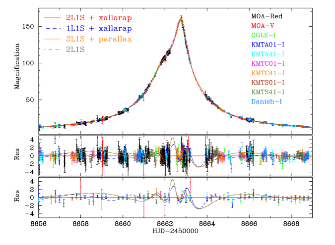
Figure 1: (Top panel) Light curve for OGLE-2019-BLG-0825. Error bars are renormalized according to Equation (1). The red solid, blue dashed, orange solid, and green dashed lines are the best 2L1S + xallarap model, the best 1L1S + xallarap model, the best 2L1S + parallax model and the best standard 2L1S model described in Section 4, respectively. (Middle panel) Residuals from the best 2L1S + xallarap model. (Bottom panel) Residuals from the best 2L1S + xallarap model binned by 0.2 days.

Table 1: Data Sets for OGLE-2019-BLG-0825

Observatory Sites	Telescope	Collaboration	Label	Filter	$N_{\rm use}$	$k$	$e_{\rm min}$
Mount John	MOA-II 1.8m	MOA	MOA	MOA-Red	3949	1.330	0.009
				$V$	86	0.835	0
Las Campanas	Warsaw 1.3m	OGLE	OGLE	$I$	1535	1.453	0.007
Siding Spring	KMTNet Australia 1.6m	KMTNet	KMTA01	$I$	704	1.649	0
			KMTA41	$I$	719	1.613	0
Cerro Tololo Inter-American	KMTNet Chile 1.6m		KMTC01	$I$	952	0.761	0.004
			KMTC41	$I$	954	1.436	0
South Africa Astronomical	KMTNet South Africa 1.6m		KMTS01	$I$	881	1.490	0
			KMTS41	$I$	887	1.416	0
ESO’s La Silla	Danish 1.54m	MiNDSTEp	Danish	$I$	76	0.706	0

Microlensing event OGLE-2019-BLG-0825 was first discovered on June 3, 2019 (${\rm HJD}^{\prime}\sim 8638$) at J2000 equatorial coordinates $({\rm R.A.,decl.})=(17^{h}52^{m}21^{s}.62,-30^{\circ}48^{\prime}13^{\prime\prime}.2)$ corresponding to Galactic coordinates $(l,b)=(-0.849,-2.214)$, by the Optical Gravitational Lensing Experiment (OGLE; Udalski, 2003) collaboration. OGLE conducts a microlensing survey using the 1.3m Warsaw Telescope with a 1.4 deg² field-of-view (FOV) CCD camera at Las Campanas Observatory in Chile and distributes alerts of the discovery of microlensing events by their OGLE-IV Early Warning System (Udalski et al., 1994; Udalski, 2003; Udalski et al., 2015). The event is located in the OGLE-IV field BLG534, which is observed on Cousins $I$-band with an hourly cadence (Mróz et al., 2019).

The Microlensing Observations in Astrophysics (MOA; Bond et al., 2001; Sumi et al., 2003) collaboration also independently discovered this event on June 23, 2019, and identified it as MOA-2019-BLG-273 using the MOA alert system (Bond et al., 2001). The MOA collaboration conducts a microlensing exoplanet survey toward the Galactic bulge using the 1.8m MOA-II telescope with a 2.2 deg² wide FOV CCD camera, MOA-cam3 (Sako et al., 2008), at the University of Canterbury’s Mount John Observatory in New Zealand. The MOA survey uses a custom wide band filter referred to as $R_{\rm MOA}$ corresponding to the sum of the Cousins $R$ and $I$ bands. In addition, a Johnson $V$-band filter is used primarily for measuring the color of the source. The event is located in the MOA field gb4, which is observed with high cadence once every 15 minutes.

The Korea Microlensing Telescope Network (KMTNet; Kim et al., 2016) collaboration conducts a microlensing survey using three 1.6m telescopes each with a 4.0 deg² FOV CCD camera. The telescopes are located at the Cerro Tololo Inter-American Observatory (CTIO) in Chile, the South African Astronomical Observatory (SAAO) in South Africa, and Siding Spring Observatory (SSO) in Australia. This event is located in an overlapping region with two KMTNet observed fields (KMTNet BLG01 and BLG41), which are observed with high cadence once every 15 minutes and was discovered by the KMTNet EventFinder (Kim et al., 2018) as KMT-2019-BLG-1389 on June 28, 2019.

The Danish telescope of MiNDSTEp (Microlensing Network for the Detection of Small Terrestrial Exoplanets) made follow-up observations in $I$-band. MiNDSTEp uses the 1.54m Danish Telescope at the European Southern Observatory at La Silla Observatory in Chile (Dominik et al., 2010). Data from the Spitzer space telescope (Yee et al., 2015) were also available, but these show no detectable signal and so are not used. A summary of all datasets used in the analysis of OGLE-2019-BLG-0825 is shown in Table 1.

The above data sets are used in our light curve analysis. To reduce long-term systematics on the baseline, we used approximately 2 years of data over $8100\leq{\rm HJD}^{\prime}\leq 8800$. Figure 1 shows the light curve of OGLE-2019-BLG-0825 and the standard binary lens single source model (hereafter, standard 2L1S), the binary lens single source with parallax effect model (hereafter, 2L1S + parallax), the single lens single source with xallarap effct model (hereafter 1L1S + xallarap), and the best-fit model (binary lens single source with xallarap effect model, hearafter 2L1S + xallarap), described in Section 4, respectively. As will be discussed in detail in Section 5, the xallarap model analysis assumes that the magnified flux of the second source is too weak to be detected, so it is denoted 1S.

3 Data Reduction

The OGLE data were reduced with the OGLE Difference Image Analysis (DIA) (Wozniak, 2000) photometry pipeline (Udalski, 2003; Udalski et al., 2015) which uses the DIA technique (Tomaney & Crotts, 1996; Alard & Lupton, 1998; Alard, 2000). The MOA data were reduced with MOA’s implementation of the DIA photometry pipeline (Bond et al., 2001). The KMTNet data were reduced with their PySIS photometry pipeline (Albrow et al., 2009). The MiNDSTEp data were reduced using DanDIA (Bramich, 2008; Bramich et al., 2013).

It is known that the nominal error bars calculated by the pipelines are incorrectly estimated in such crowded stellar fields. We follow a standard empirical error bar normalization process (Yee et al., 2012) intended to estimate proper uncertainties for the lensing parameters in the light-curve modeling. This process, described below, hardly affects the best-fit parameters (Ranc et al., 2019). We renormalize the photometric error bars using the formula

$$\sigma^{\prime}_{i}=k\sqrt{\sigma^{2}_{i}+e^{2}_{\rm min}},$$ (1)

in which $\sigma^{\prime}_{i}$ is the renormalized uncertainty in magnitude, while $\sigma_{i}$ is an uncertainty of the $i$-th original data point obtained from the photometric pipeline. The variables $k$ and $e_{\rm min}$ are renormalizing parameters. For preliminary modeling, we search for the best-fit lensing parameters using $\sigma_{i}$. We then construct a cumulative $\chi^{2}$ distribution as a function of lensing magnification. The $e_{\rm min}$ value is chosen so that the slope of the distribution is uniform (Yee et al., 2012). The $k$ value is chosen so that $\chi^{2}/$d.o.f.$\simeq 1$. In Table 1, we list the calculated error bar renormalization parameters.

4 Light Curve Modeling

The model flux for a microlensing event is given by the following equation,

$$f(t)=A(t,\bm{x})f_{s}+f_{b},$$ (2)

where $A(t,\bm{x})$ is the source flux magnification, $f_{s}$ is the flux of the source star, and $f_{b}$ is the blend flux. In the 1L1S model, $\bm{x}$ is described by four parameters (Paczynski, 1986): the time of the source closest to the center of mass, $t_{0}$; the Einstein radius crossing time, $t_{\rm E}$; the impact parameter, $u_{0}$, and the source angular radius, $\rho$. Both $u_{0}$ and $\rho$ are in units of the angular Einstein radius, $\theta_{\rm E}$.

For modeling the light curve, we used the Metropolis-Hastings Markov Chain Monte Carlo method. The finite source effect, an effect in which the source has a finite angular size, was calculated using the image-centered inverse-ray shooting method (Bennett & Rhie, 1996; Bennett, 2010) as implemented by Sumi et al. (2010). Note that $f_{s}$ and $f_{b}$ parameters are obtained from a linear-fit using the method of Rhie et al. (1999). We adopt the following linear limb-darkening law for source brightness:

$$S_{\lambda}(\vartheta)=S_{\lambda}(0)\left[1-u_{\lambda}(1-\cos(\vartheta))\right],$$ (3)

where $\vartheta$ represents the angle between the line of sight and the normal to the surface of the source star. $S_{\lambda}(\vartheta)$ is a limb-darkening surface brightness of $\vartheta$ at wavelength $\lambda$. We estimated the effective temperature of the source star in Section 5 to be $T_{\rm eff}=5425\pm 359$ K (González Hernández & Bonifacio, 2009). In this analysis, we assume the source star’s metallicity $[\rm M/H]=0$, surface gravity $\log{g}=4.5$, and microturbulent velocity $v=1$ $\rm{km/s}$. We use the limb-darkening cofficients $u_{V}=0.685$, $u_{R}=0.604$ and $u_{I}=0.518$, which are taken from the ATLAS model with $T_{\rm eff}=5500$ K (Claret & Bloemen, 2011). Since $R_{\rm MOA}$ covers both $R$- and $I$-band wavelengths, we adopted the average value $u_{R_{\rm MOA}}=(u_{R}+u_{I})/2=0.561$. In addition, as will be discussed in more detail in Section 7, we assume that the source of this event is a main-sequence star.

As the result of 1L1S model analysis, we found that $(t_{0},t_{\rm E},u_{0},\rho)=(8662.6,47.6,1.2\times 10^{-2},4.8\times 10^{-3})$ is the best solution. This 1L1S best model is $\Delta\chi^{2}=21400$ worse than the best standard 2L1S model.

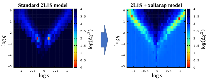
Figure 2: Map of $\Delta\chi^{2}$ in each $s–q$ grid from the $(q,s,\alpha)$ grid search for the standard 2L1S model (Left) and for the 2L1S + xallarap model (Right). The best fit $\alpha$ is chosen for each grid location, respectively. In the map of the standard 2L1S model, we found the best solution at $q\sim 10^{-3}$. However, for the 2L1S + xallarap map, best solutions at two other local minima appear at $q>0.1$.

Figure 3: (Top panel) Light curve for OGLE-2019-BLG-0825. Error bars are renormalized according to Equation (1). The solid red, dashed blue, and solid orange lines, dashed green are the standard 2L1S close1 model, standard 2L1S wide1 model, standard 2L1S close2 model, and standard 2L1S wide2 model, respectively. (Middle panel) Zoom of $8661<{\rm HJD}-245000<8665$. (Bottom panel) Residuals from the best of standard 2L1S (i.e. close1) model.

4.1 Standard Binary Lens

In the standard 2L1S model, three additional parameters are required; the mass ratio of a lens companion relative to the host, $q$; the projected separation normalized by Einstein radius between binary components, $s$; the angle between the binary-lens axis and the source trajectory direction, $\alpha$.

Because the $\chi^{2}$ surface of the microlensing parameter has a very complicated shape, 34440 values of $(q,s,\alpha)$, which have a particularly large impact on the shape of the light curve were initially fixed in the fitting process. Here we uniformly take 21 values between $-5\leq\log{q}\leq 0$, 41 values between $-1.25\leq\log{s}\leq 1.25$, 40 values in $0\leq\alpha\leq 2\pi$, respectively. For the top 1000 combinations which gave good fits, we performed the fitting again with $q,s$, and $\alpha$ free. This process minimizes the chance that we miss local solutions even in a large and complex microlensing parameter space. The left panel of Figure 2 shows the results of the grid search analysis for the standard 2L1S model.

As a result of the analysis, the best fit standard 2L1S model is $(q,s)=(3.3\times 10^{-3},0.57)$ (close1). Hereafter, we call solutions with $s<1$ and $s>1$ as “close” and “wide”, respectively. We call the best standard 2L1S as close1. We also found local minima at $(q,s)=(3.4\times 10^{-3},1.75)$ (wide1) with $\Delta\chi^{2}\sim 0.4$, $(q,s)=(2.1\times 10^{-2},0.28)$ (close2) with $\Delta\chi^{2}\sim 20.4$ and $(q,s)=(2.1\times 10^{-2},3.78)$ (wide2) with $\Delta\chi^{2}\sim 23.3$. Detailed parameters of the standard binary models are shown in Table 3. However, we observed systematic residuals around the peak of $8657<{\rm HJD}^{\prime}<8667$ in these models, as depicted by the green dashed line in Figure 1. In Figure 1, we plot only close1, the best for the standard 2L1S, but the other three models also have similar residuals. We therefore proceed to model the light curve with higher order effects.

Table 2: Parameters of the standard 2L1S models

Model	close1	close2	wide1	wide2
$t_{0}$(HJD-2458660)	$2.474\pm 0.001$	$2.483\pm 0.001$	$2.473\pm 0.001$	$2.489\pm 0.001$
$t_{\rm E}$ (days)	$74.7\pm 2.0$	$75.7\pm 2.0$	$72.8\pm 1.8$	$77.3\pm 2.0$
$u_{0}$ ($10^{-3}$)	$7.30\pm 0.21$	$7.11\pm 0.19$	$7.53\pm 0.19$	$6.91\pm 0.19$
$q$ ($10^{-3}$)	$3.30\pm 0.11$	$20.71\pm 9.84$	$3.39\pm 0.10$	$21.33\pm 1.15$
$s$	$0.569\pm 0.004$	$0.207\pm 0.038$	$1.747\pm 0.011$	$3.776\pm 0.063$
$\alpha$ (radian)	$5.034\pm 0.002$	$2.766\pm 0.002$	$5.036\pm 0.003$	$2.767\pm 0.002$
$\rho$ ($10^{-3}$)	$2.95\pm 0.09$	$0.48\pm 0.28$	$3.02\pm 0.09$	$0.47\pm 0.14$
$\chi^{2}$	11744.7	11765.1	11745.1	11768.0
$\Delta\chi^{2}$	-	20.4	0.4	23.3

Table 3: Parameters of the standard 2L1S models

Model	close1	close2	wide1	wide2
$t_{0}$(HJD-2458660)	$2.474\pm 0.001$	$2.483\pm 0.001$	$2.473\pm 0.001$	$2.489\pm 0.001$
$t_{\rm E}$ (days)	$74.73\pm 2.01$	$75.73\pm 1.980$	$72.79\pm 1.79$	$77.33\pm 2.03$
$u_{0}$ ($10^{-3}$)	$7.300\pm 0.210$	$7.110\pm 0.189$	$7.528\pm 0.189$	$6.910\pm 0.187$
$q$ ($10^{-3}$)	$3.301\pm 0.114$	$20.710\pm 9.839$	$3.387\pm 0.102$	$21.334\pm 1.145$
$s$	$0.569\pm 0.004$	$0.207\pm 0.038$	$1.747\pm 0.011$	$3.776\pm 0.063$
$\alpha$ (radian)	$5.034\pm 0.002$	$2.766\pm 0.002$	$5.036\pm 0.003$	$2.767\pm 0.002$
$\rho$ ($10^{-3}$)	$2.950\pm 0.093$	$0.481\pm 0.278$	$3.018\pm 0.092$	$0.471\pm 0.141$
$\chi^{2}$	11744.7	11765.1	11745.1	11768.0
$\Delta\chi^{2}$	-	20.4	0.4	23.3

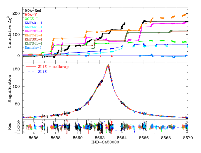
Figure 4: (Top panel) Cumulative $\Delta\chi^{2}$ for the xallarap model compared to the standard binary lens model. Each color corresponds to each instrument listed the left side of the axes. (Middle panel) The light curve of the best 2L1S + xallarap model (solid red line), and the light curve of the standard 2L1S best model (blue dashed line). (Bottom panel) Residuals of the light curves from the 2L1S + xallarap model.

Table 4: Parameters of the 2L1S + xallarap models, 1L1S + xallarap model, and 1L1S + xallarap + parallax model

Model	XLclose1	XLclose2	XLwide1	XLwide2	1LXL	1LXLPL
range of $q$	$q\leq 0.1$	$0.1<q\leq 1$	$q\leq 0.1$	$0.1<q\leq 1$	-	-
$t_{0}$(HJD-2458660)	$2.576\pm 0.005$	$2.573\pm 0.007$	$2.572\pm 0.004$	$2.575\pm 0.006$	$2.744\pm 0.001$	$2.744\pm 0.001$
$t_{\rm E}$ (days)	$97.7\pm 2.6$	$93.8\pm 3.1$	$100.7\pm 3.4$	$133.3\pm 11.5$	$67.2\pm 2.0$	$73.5\pm 1.5$
$u_{0}$ ($10^{-3}$)	$-7.16\pm 0.22$	$-6.98\pm 0.21$	$7.06\pm 0.21$	$4.91\pm 0.35$	$6.93\pm 0.20$	$6.31\pm 0.14$
$q$	$0.09\pm 0.01$	$0.44\pm 0.11$	$0.10\pm 0.01$	$0.94\pm 0.37$	-	-
$s$	$0.141\pm 0.004$	$0.085\pm 0.004$	$7.403\pm 0.438$	$18.040\pm 1.263$	-	-
$\alpha$ (radian)	$0.429\pm 0.008$	$1.937\pm 0.010$	$5.846\pm 0.008$	$4.350\pm 0.009$	-	-
$\rho$ ($10^{-3}$)	$2.56\pm 0.13$	$2.15\pm 0.12$	$2.41\pm 0.11$	$1.44\pm 0.16$	$7.04\pm 0.20$	$6.41\pm 0.14$
${\rm RA}_{\xi}$ (degree)	$81.6\pm 11.7$	$153.2\pm 10.5$	$75.9\pm 14.5$	$155.4\pm 8.5$	$31.3\pm 0.5$	$32.1\pm 0.5$
${\rm decl}_{\xi}$ (degree)	$54.5\pm 10.5$	$36.9\pm 16.4$	$-79.4\pm 12.8$	$-40.7\pm 14.1$	$9.9\pm 0.2$	$9.9\pm 0.3$
$P_{\xi}$ (days)	$5.42\pm 0.04$	$5.53\pm 0.05$	$5.43\pm 0.04$	$5.54\pm 0.05$	$2.91\pm 0.02$	$2.9\pm 0.02$
$\xi_{{\rm E,N}}$ ($10^{-3}$)	$1.82\pm 0.15$	$-0.36\pm 0.36$	$-1.65\pm 0.11$	$0.34\pm 0.20$	$-3.59\pm 0.11$	$-3.23\pm 0.08$
$\xi_{{\rm E,E}}$ ($10^{-3}$)	$0.69\pm 0.34$	$1.53\pm 0.12$	$0.42\pm 0.41$	$1.07\pm 0.10$	$2.86\pm 0.09$	$2.58\pm 0.07$
$\pi_{{\rm E,N}}$	-	-	-	-	-	$0.09\pm 0.05$
$\pi_{{\rm E,E}}$	-	-	-	-	-	$0.26\pm 0.14$
$\chi^{2}$	10856.4	10840.9	10861.2	10842.7	11311.5	11285.7
$\Delta\chi^{2}$	15.5	-	20.3	1.8	470.6	444.8

Table 5: Parameters of the 2L1S + xallarap models, 1L1S + xallarap model, and 1L1S + xallarap + parallax model

Model	XLclose1	XLclose2	XLwide1	XLwide2	1LXL	1LXLPL
range of $q$	$q\leq 0.1$	$0.1<q\leq 1$	$q\leq 0.1$	$0.1<q\leq 1$	-	-
$t_{0}$(HJD-2458660)	$2.576\pm 0.005$	$2.573\pm 0.007$	$2.572\pm 0.004$	$2.575\pm 0.006$	$2.744\pm 0.001$	$2.744\pm 0.001$
$t_{\rm E}$ (days)	$97.70\pm 2.63$	$93.75\pm 3.09$	$100.65\pm 3.39$	$133.28\pm 11.48$	$67.21\pm 2.04$	$73.46\pm 1.50$
$u_{0}$ ($10^{-3}$)	$-7.159\pm 0.216$	$-6.976\pm 0.213$	$7.064\pm 0.215$	$4.915\pm 0.350$	$6.927\pm 0.196$	$6.312\pm 0.139$
$q$	$0.094\pm 0.006$	$0.437\pm 0.110$	$0.098\pm 0.011$	$0.943\pm 0.370$	-	-
$s$	$0.141\pm 0.004$	$0.085\pm 0.004$	$7.403\pm 0.438$	$18.040\pm 1.263$	-	-
$\alpha$ (radian)	$0.429\pm 0.008$	$1.937\pm 0.010$	$5.846\pm 0.008$	$4.350\pm 0.009$	-	-
$\rho$ ($10^{-3}$)	$2.562\pm 0.134$	$2.154\pm 0.125$	$2.409\pm 0.111$	$1.443\pm 0.156$	$7.039\pm 0.198$	$6.415\pm 0.144$
${\rm RA}_{\xi}$ (degree)	$81.56\pm 11.72$	$153.20\pm 10.46$	$75.86\pm 14.53$	$155.44\pm 8.50$	$31.31\pm 0.50$	$32.13\pm 0.54$
${\rm decl}_{\xi}$ (degree)	$54.53\pm 10.51$	$36.93\pm 16.38$	$-79.41\pm 12.83$	$-40.69\pm 14.05$	$9.88\pm 0.24$	$9.89\pm 0.26$
$P_{\xi}$ (days)	$5.417\pm 0.042$	$5.531\pm 0.046$	$5.433\pm 0.035$	$5.538\pm 0.046$	$2.909\pm 0.021$	$2.89\pm 0.02$
$\xi_{{\rm E,N}}$ ($10^{-3}$)	$1.818\pm 0.150$	$-0.363\pm 0.359$	$-1.646\pm 0.106$	$0.337\pm 0.195$	$-3.592\pm 0.106$	$-3.233\pm 0.082$
$\xi_{{\rm E,E}}$ ($10^{-3}$)	$0.691\pm 0.343$	$1.533\pm 0.118$	$0.419\pm 0.410$	$1.073\pm 0.102$	$2.860\pm 0.089$	$2.576\pm 0.074$
$\pi_{{\rm E,N}}$ ($10^{-2}$)	-	-	-	-	-	$9.272\pm 5.359$
$\pi_{{\rm E,E}}$ ($10^{-1}$)	-	-	-	-	-	$2.576\pm 1.375$
$\chi^{2}$	10856.4	10840.9	10861.2	10842.7	11311.5	11285.7
$\Delta\chi^{2}$	15.5	-	20.3	1.8	470.6	444.8

Table 6: Parameters of the 2L1S + xallarap models

Model	XLclose1	XLclose2	XLclose3	XLwide1	XLwide2	XLwide3
range of $q$	$q\leq 0.1$	$0.1<q\leq 0.5$	$0.5<q\leq 1$	$q\leq 0.1$	$0.1<q\leq 0.5$	$0.5<q\leq 1$
$t_{0}$(HJD-2458660)	$2.576\pm 0.005$	$2.573\pm 0.007$	$2.566\pm 0.007$	$2.572\pm 0.004$	$2.583\pm 0.005$	$2.575\pm 0.006$
$t_{\rm E}$ (days)	$97.70\pm 2.63$	$93.75\pm 3.09$	$95.50\pm 2.71$	$100.65\pm 3.39$	$115.66\pm 5.26$	$133.28\pm 11.48$
$u_{0}$ ($10^{-3}$)	$-7.159\pm 0.216$	$-6.976\pm 0.213$	$6.880\pm 0.186$	$7.064\pm 0.215$	$5.627\pm 0.239$	$4.915\pm 0.350$
$q$	$0.094\pm 0.006$	$0.437\pm 0.110$	$0.632\pm 0.169$	$0.098\pm 0.011$	$0.474\pm 0.129$	$0.943\pm 0.370$
$s$	$0.141\pm 0.004$	$0.085\pm 0.004$	$0.079\pm 0.003$	$7.403\pm 0.438$	$14.535\pm 1.151$	$18.040\pm 1.263$
$\alpha$ (radian)	$0.429\pm 0.008$	$1.937\pm 0.010$	$4.335\pm 0.010$	$5.846\pm 0.008$	$4.362\pm 0.008$	$4.350\pm 0.009$
$\rho$ ($10^{-3}$)	$2.562\pm 0.134$	$2.154\pm 0.125$	$2.118\pm 0.153$	$2.409\pm 0.111$	$1.722\pm 0.110$	$1.443\pm 0.156$
${\rm RA}_{\xi}$ (degree)	$81.56\pm 11.72$	$153.20\pm 10.46$	$153.54\pm 11.83$	$75.86\pm 14.53$	$161.96\pm 15.07$	$155.44\pm 8.50$
${\rm decl}_{\xi}$ (degree)	$54.53\pm 10.51$	$36.93\pm 16.38$	$-36.05\pm 16.87$	$-79.41\pm 12.83$	$-43.57\pm 15.12$	$-40.69\pm 14.05$
$P_{\xi}$ (days)	$5.417\pm 0.042$	$5.531\pm 0.046$	$5.552\pm 0.050$	$5.433\pm 0.035$	$5.520\pm 0.050$	$5.538\pm 0.046$
$\xi_{{\rm E,N}}$ ($10^{-3}$)	$1.818\pm 0.150$	$-0.363\pm 0.359$	$0.272\pm 0.369$	$-1.646\pm 0.106$	$0.643\pm 0.241$	$0.337\pm 0.195$
$\xi_{{\rm E,E}}$ ($10^{-3}$)	$0.691\pm 0.343$	$1.533\pm 0.118$	$1.524\pm 0.109$	$0.419\pm 0.410$	$1.139\pm 0.224$	$1.073\pm 0.102$
$\chi^{2}$	10856.4	10840.9	10842.3	10861.2	10843.4	10842.7
$\Delta\chi^{2}$	15.5	-	1.3	20.3	2.4	1.8

Table 7: Parameters of the 2L1S + xallarap wide models

Model	XLwide1	XLwide2	XLwide3	XLwide4
range of $q$	$q\leq 0.05$	$0.05<q\leq 0.1$	$0.1<q\leq 0.5$	$0.5<q\leq 1$
$t_{0}$(HJD-2458660)	$2.669\pm 0.011$	$2.656\pm 0.003$	$2.583\pm 0.003$	$2.574\pm 0.004$
$t_{\rm E}$ (days)	$98.1\pm 2.1$	$98.8\pm 3.1$	$115.7\pm 1.5$	$131.5\pm 5.5$
$u_{0}$ ($10^{-3}$)	$-6.49\pm 0.14$	$-6.33\pm 0.19$	$5.62\pm 0.06$	$5.00\pm 0.21$
$q$	$0.042\pm 0.002$	$0.092\pm 0.008$	$0.474\pm 0.048$	$0.915\pm 0.172$
$s$	$5.520\pm 0.170$	$8.004\pm 0.465$	$14.535\pm 0.368$	$17.777\pm 0.731$
$\alpha$ (radian)	$0.324\pm 0.020$	$0.303\pm 0.010$	$4.362\pm 0.006$	$4.349\pm 0.006$
$\rho$ ($10^{-3}$)	$2.61\pm 0.19$	$2.56\pm 0.15$	$1.72\pm 0.08$	$1.47\pm 0.05$
${\rm RA}_{\xi}$ (degree)	$72.0\pm 1.7$	$251.3\pm 1.6$	$162.0\pm 8.8$	$153.7\pm 9.3$
${\rm decl}_{\xi}$ (degree)	$10.2\pm 1.4$	$10.8\pm 0.8$	$-43.6\pm 6.7$	$-35.4\pm 7.5$
$P_{\xi}$ (days)	$5.317\pm 0.059$	$5.412\pm 0.046$	$5.520\pm 0.040$	$5.536\pm 0.032$
$\xi_{{\rm E,N}}$ ($10^{-3}$)	$4.898\pm 0.329$	$-4.477\pm 0.231$	$0.643\pm 0.236$	$0.323\pm 0.192$
$\xi_{{\rm E,E}}$ ($10^{-3}$)	$1.672\pm 0.193$	$-1.535\pm 0.101$	$1.139\pm 0.111$	$1.105\pm 0.105$
$\chi^{2}$	10869.9	10863.1	10843.4	10843.1
$\Delta\chi^{2}$	28.9	22.2	2.4	2.1

Table 8: Parameters of the 2L1S + xallarap close models

Model	XLclose1	XLclose2	XLclose3	XLclose4
range of $q$	$q\leq 0.05$	$0.05<q\leq 0.1$	$0.1<q\leq 0.5$	$0.5<q\leq 1$
$t_{0}$(HJD-2458660)	$2.664\pm 0.008$	$2.568\pm 0.002$	$2.573\pm 0.006$	$2.566\pm 0.004$
$t_{\rm E}$ (days)	$92.5\pm 2.9$	$98.0\pm 1.6$	$93.75\pm 2.79$	$95.5\pm 2.4$
$u_{0}$ ($10^{-3}$)	$6.87\pm 0.20$	$-7.18\pm 0.12$	$-6.98\pm 0.20$	$6.88\pm 0.17$
$q$	$0.047\pm 0.003$	$0.099\pm 0.81$	$0.437\pm 0.096$	$0.632\pm 0.080$
$s$	$0.179\pm 0.007$	$0.139\pm 0.005$	$0.085\pm 0.005$	$0.079\pm 0.002$
$\alpha$ (radian)	$5.964\pm 0.013$	$0.436\pm 0.004$	$1.937\pm 0.009$	$4.335\pm 0.007$
$\rho$ ($10^{-3}$)	$2.70\pm 0.15$	$2.54\pm 0.07$	$2.15\pm 0.14$	$2.12\pm 0.11$
${\rm RA}_{\xi}$ (degree)	$71.4\pm 1.5$	$91.5\pm 8.9$	$153.2\pm 8.6$	$153.5\pm 4.1$
${\rm decl}_{\xi}$ (degree)	$-9.7\pm 8.9$	$72.6\pm 10.7$	$36.9\pm 15.4$	$-36.0\pm 9.6$
$P_{\xi}$ (days)	$5.386\pm 0.035$	$5.438\pm 0.022$	$5.531\pm 0.052$	$5.55\pm 0.05$
$\xi_{{\rm E,N}}$ ($10^{-3}$)	$-5.279\pm 0.314$	$1.472\pm 0.132$	$-0.363\pm 0.328$	$0.272\pm 0.166$
$\xi_{{\rm E,E}}$ ($10^{-3}$)	$1.765\pm 0.139$	$0.870\pm 0.224$	$1.533\pm 0.093$	$1.524\pm 0.086$
$\chi^{2}$	10866.1	10856.9	10842.5	10842.3
$\Delta\chi^{2}$	25.2	15.9	-	1.3

Table 9: Parameters of the 2L1S + xallarap wide models

Model	XLwide1	XLwide2	XLwide3	XLwide4
range of $q$	$q\leq 0.001$	$0.001<q\leq 0.01$	$0.01<q\leq 0.1$	$0.1<q\leq 1$
$t_{0}$(HJD-2458660)	$2.744\pm 0.001$	$2.125\pm 0.012$	$2.670\pm 0.016$	$2.597\pm 0.011$
$t_{\rm E}$ (days)	$56.3\pm 0.8$	$114.6\pm 3.2$	$98.0\pm 2.1$	$105.1\pm 2.0$
$u_{0}$ ($10^{-3}$)	$-9.14\pm 0.03$	$9.82\pm 0.26$	$-7.32\pm 0.13$	$6.78\pm 0.24$
$q$ ($10^{-3}$)	$0.774\pm 0.022$	$6.51\pm 0.33$	$29.2\pm 2.1$	$114\pm 30$
$s$	$1.206\pm 0.001$	$2.319\pm 0.036$	$4.362\pm 0.169$	$8.286\pm 1.059$
$\alpha$ (radian)	$5.835\pm 0.003$	$5.542\pm 0.014$	$0.340\pm 0.025$	$0.376\pm 0.021$
$\rho$ ($10^{-3}$)	$9.41\pm 0.08$	$4.35\pm 0.13$	$2.26\pm 0.16$	$2.07\pm 0.15$
${\rm RA}_{\xi}$ (degree)	$31.8\pm 0.6$	$86.6\pm 3.2$	$73.2\pm 11.2$	$62.0\pm 17.6$
${\rm decl}_{\xi}$ (degree)	$4.5\pm 0.3$	$-26.1\pm 2.3$	$25.0\pm 3.6$	$47.7\pm 5.3$
$P_{\xi}$ (days)	$4.65\pm 0.03$	$5.38\pm 0.04$	$5.40\pm 0.05$	$5.51\pm 0.05$
$e_{\xi}$ ($10^{-1}$)	$5.34\pm 0.06$	$5.38\pm 0.08$	$2.07\pm 0.21$	$1.54\pm 0.29$
$T_{\rm peri}$ (HJD-2458600)	$62.54\pm 0.01$	$67.69\pm 0.04$	$62.68\pm 0.13$	$57.43\pm 0.16$
$\xi_{{\rm E,N}}$ ($10^{-3}$)	$3.16\pm 0.02$	$-4.33\pm 0.16$	$3.16\pm 0.23$	$1.78\pm 0.22$
$\xi_{{\rm E,E}}$ ($10^{-3}$)	$2.90\pm 0.10$	$-1.09\pm 0.13$	$1.23\pm 0.13$	$0.91\pm 0.38$
$\chi^{2}$	10829.1	10831.6	10824.7	10830.5
$\Delta\chi^{2}$	4.4	6.9	-	5.8

Table 10: Parameters of the 2L1S + xallarap close models

Model	XLclose1	XLclose2	XLclose3	XLclose4
range of $q$	$q\leq 0.001$	$0.001<q\leq 0.01$	$0.01<q\leq 0.1$	$0.1<q\leq 1$
$t_{0}$(HJD-2458660)	$2.791\pm 0.007$	$2.860\pm 0.007$	$2.670\pm 0.015$	$2.605\pm 0.014$
$t_{\rm E}$ (days)	$83.1\pm 2.2$	$71.0\pm 1.6$	$96.0\pm 2.2$	$98.5\pm 2.9$
$u_{0}$ ($10^{-3}$)	$6.56\pm 0.18$	$-7.30\pm 0.15$	$-7.46\pm 0.26$	$7.17\pm 0.21$
$q$ ($10^{-3}$)	$0.955\pm 0.179$	$6.85\pm 0.82$	$27.4\pm 3.9$	$103\pm 16$
$s$	$0.586\pm 0.020$	$0.429\pm 0.020$	$0.239\pm 0.018$	$0.132\pm 0.008$
$\alpha$ (radian)	$4.068\pm 0.021$	$6.134\pm 0.019$	$0.343\pm 0.026$	$0.362\pm 0.021$
$\rho$ ($10^{-3}$)	$1.10\pm 0.46$	$4.42\pm 0.28$	$2.31\pm 0.18$	$2.22\pm 0.16$
${\rm RA}_{\xi}$ (degree)	$67.6\pm 10.6$	$260.5\pm 4.2$	$83.4\pm 10.4$	$245.3\pm 16.1$
${\rm decl}_{\xi}$ (degree)	$-50.7\pm 7.5$	$28.2\pm 3.5$	$25.4\pm 3.4$	$44.3\pm 12.2$
$P_{\xi}$ (days)	$5.48\pm 0.05$	$5.36\pm 0.04$	$5.44\pm 0.06$	$5.50\pm 0.05$
$e_{\xi}$ ($10^{-1}$)	$5.66\pm 0.26$	$5.39\pm 0.14$	$2.08\pm 0.24$	$1.73\pm 0.34$
$T_{\rm peri}$ (HJD-2458600)	$62.36\pm 0.02$	$56.97\pm 0.04$	$62.56\pm 0.11$	$51.80\pm 0.18$
$\xi_{{\rm E,N}}$ ($10^{-3}$)	$-2.51\pm 0.16$	$-3.75\pm 0.13$	$3.18\pm 0.23$	$-1.98\pm 0.34$
$\xi_{{\rm E,E}}$ ($10^{-3}$)	$0.90\pm 0.44$	$-2.55\pm 0.23$	$1.26\pm 0.13$	$-0.85\pm 0.29$
$\chi^{2}$	10836.8	10831.4	10825.3	10830.7
$\Delta\chi^{2}$	12.2	6.8	0.6	6.0

4.2 Parallax

It is known that the acceleration of Earth orbital motion affects the light curve of microlensing events (Gould, 1992, 2004; Smith et al., 2003; Dong et al., 2009). This parallax effect can be described by the microlensing parallax vector $\bm{\pi_{\rm E}}=(\pi_{{\rm E,N}},\pi_{{\rm E,E}})$ where $\pi_{{\rm E,N}}$ and $\pi_{{\rm E,E}}$ represents respectively the north and east components of $\bm{\pi_{\rm E}}$ projected onto the sky plane in equatorial coordinates. The direction of $\bm{\pi_{\rm E}}$ is defined to coincide with the direction of the geocentric lens-source relative proper motion projected onto the sky plane at the reference time $t_{\rm fix}$, and the amplitude of $\bm{\pi_{\rm E}}$ is $\pi_{\rm E}={\rm au}/\tilde{r}_{\rm E}$ ($\tilde{r}_{\rm E}$ is the Einstein radius projected inversely to the observation plane) (Gould, 2000).

As a result of modeling by adding two parameters of $\pi_{{\rm E,N}}$ and $\pi_{{\rm E,E}}$, we found two degenerate models with $(q,s)=(3.5\times 10^{-3},0.57)$ and $(q,s)=(3.4\times 10^{-3},1.74)$, that are better than the standard 2L1S model by $\Delta\chi^{2}=68.3$. However, the cumulative $\Delta\chi^{2}$ improvement for parallax model relative to standard 2L1S model is not consistent between the data sets. Furthermore, we still found systematic residuals around the peak of $8657<{\rm HJD}^{\prime}<8667$ in these models, as seen in the standard 2L1S model shown by the orange solid line in Figure 1.

4.3 Xallarap

We next consider the possibility that the short term residuals in $8657<{\rm HJD}^{\prime}<8667$ are caused by a short period binary source system, i.e., they arise owing to the xallarap effect.

The xallarap effect can be described by the following seven parameters; the direction toward the solar system relative to the orbital plane of the source system, ${\rm RA}_{\xi}$ and ${\rm decl}_{\xi}$; the source orbital period, $P_{\xi}$; the source orbital eccentricity $e_{\xi}$; the perihelion $T_{\rm peri}$; the xallarap vector, $\bm{\xi_{\rm E}}=(\xi_{{\rm E,N}},\xi_{{\rm E,E}})$. Note that this effect does not include the magnifying effect of the source companion star; only the source host contributes to the magnification. We denote this model of the microlensing event as the 2L1S + xallarap model rather than as the 2L2S model to distinguish it from a model including secondary source magnification. As discussed in detail in Section 5, the flux ratio of the source companion to the host star in the $I$-band in the best 2L1S + xallarap model is $\sim 10^{-7}$. Therefore, we assume that the brightening of the source companion star is negligible.

We first fit using 78,960 values of xallarap parameters $({\rm RA}_{\xi},{\rm decl}_{\xi},P_{\xi})$ with the four best standard 2L1S models (close1, wide1, close2, and wide2) as initial values. We used 20 evenly spaced values for $0\leq{\rm RA}_{\xi}<360$, 21 values for $-90\leq{\rm decl}_{\xi}<90$, 19 and 99 values for $1<P_{\xi}$ [days] $<19$ and $20<P_{\xi}$ [days] $<1000$, respectively. After that, we fit again with $({\rm RA}_{\xi},{\rm decl}_{\xi},P_{\xi})$ as free parameters. As a result, we found the best solutions with $P_{\xi}\sim 5$ days independently from the initial values of close1, wide1, close2, and wide2. We also found that the final $q$ and $s$ values are quite different from their initial values, and did not converge. Therefore, we next set $P_{\xi}\sim 5$ days as the initial value, ${\rm RA}_{\xi}$ and ${\rm decl}_{\xi}$ to random values, and performed model fitting with 34,440 values of $(q,s,\alpha)$ using the same procedure as the standard 2L1S modeling described in Section 4.1. Short-period binary stars orbiting in $P_{\xi}\sim 5$ days are affected by orbital circularization due to tidal friction (Fabrycky & Tremaine, 2007). The tidal circularization time is discussed in Section 7, but it is reasonable to assume that at the age of the stars in the Galactic bulge (Sit & Ness, 2020), the orbit is fully circularized. Therefore, we fixed the eccentricity at $e_{\xi}=0$. When $e_{\xi}=0$, $T_{\rm peri}$ can be eliminated as a fitting parameter. The results are shown in the right panel of Figure 2.

The figure shows that there are degenerate solutions for various combinations of $(q,s)$ values in the range of $\Delta\chi^{2}\lesssim 20$. Table 6 shows the best fit model parameters for the wide and close solutions. The reason for the slight difference in $\Delta\chi^{2}$ between Figure 2 and Table 6 is that the models in Table 6 were fitted with $q$, $s$, and $\alpha$ set free. We label the best models of the mass ratio range in the 2L1S + xallarap close model, respectively: the best with $q\leq 0.1$ is XLclose1, the best with $0.1<q\leq 1$ is XLclose2. Similarly, in the wide model of 2L1S + xallarap, we label the best with $q\leq 0.1$ as XLwide1, the best with $0.1<q\leq 1$ as XLwide2. Figure 1 shows the best 2L1S + xallarap model (i.e. XLclose2). The xallarap models fit the light curves better than the standard 2L1S models. The figure shows that there are degenerate solutions with various combination of $(q,s)$ values within a small range of $\Delta\chi^{2}$. Table 9 and Table 10 show the best fit model parameters in the ranges of $q\leq 0.001$, $0.001<q\leq 0.01$, $0.01<q\leq 0.1$ and $0.1<q\leq 1$ for wide and close solutions, respectively. We label the best models of the mass ratio range in the 2L1S + xallarap wide model, respectively: the best with $q\leq 0.001$ is XLwide1, the best with $0.001<q\leq 0.01$ is XLwide2, the best with $0.01<q\leq 0.1$ is XLwide3, the best with $0.1<q\leq 1$ best is XLwide4. Similarly, in the close model of 2L1S + xallarap, we label the best with $q\leq 0.001$ as XLclose1, the best with $0.001<q\leq 0.01$ as XLclose2, the best with $0.01<q\leq 0.1$ as XLclose3, and the best with $0.1<q\leq 1$ as XLclose4. Figure 1 shows the best 2L1S + xallarap model (i.e. XLwide3). The xallarap models fit the light curves better than the standard 2L1S models.

Figure 4 shows the cumulative $\Delta\chi^{2}$ of the best 2L1S + xallarap model relative to the best standard 2L1S model. One can see that the 2L1S + xallarap model improves $\chi^{2}$ around the peak of $8657<{\rm HJD}^{\prime}<8667$. The 2L1S + xallarap model improved $\chi^{2}$ by $903.7$ from the standard 2L1S model and by $835.5$ from the 2L1S + parallax model. Figure 5 shows the geometry of the primary lens, source trajectory, caustics on the magnification map for the best 2L1S + xallarap model. The short orbital period of the source star with $P_{\xi}\sim 5$ days make the source’s trajectory a wavy line.

We applied the same procedure for 1L1S and found the best 1L1S + xallarap model has $\Delta\chi^{2}=470.6$ worse than the best 2L1S + xallarap model. We label the best 1L1S + xallarap model as 1LXL. Even the 1L1S + xallarap + parallax model was $\Delta\chi^{2}=444.8$ worse than the best 2L1S + xallarap model. We label the best 1L1S + xallarap + parallax model as 1LXLPL. The parameters of each of the best models are listed in Table 13. However, asymmetric maps similar to Figure 5 can be created by binary lenses of various parameters, which led to the emergence of various degenerate 2L1S + xallarap models. We considered other higher order effects and combinations of them such as 2L1S + xallarap + parallax, 2L1S + xallarap + parallax + lens orbital motion, and 1L2S, but could not detect them significantly. For comparison with the 2L1S + xallarap model, we also fitted the 2L1S model with a variable source. In this case, the amplitude of the variation, $\gamma$; the period of the variation, $T_{\rm v}$; and the initial phase, $\beta$ are additional parameters. We fixed the other parameters at those of the best standard 2L1S model (i.e., close1). However, the $\chi^{2}$ improvement from the best standard 2L1S model was only $139.1$, $\Delta\chi^{2}=764.6$ worse than the best 2L1S + xallarap model. To confirm, we performed 2L1S + xallarap fitting analysis with $\xi_{\rm E,N}$, $\xi_{\rm E,E}$, ${\rm RA}_{\xi}$, ${\rm decl}_{\xi}$, and $P_{\xi}$ set free and the other parameters fixed to the best standard 2L1S model. As a result, the $\chi^{2}$ was improved by $594.5$ over the best standard 2L1S model. This is only $\Delta\chi^{2}=309.3$ worse than the best 2L1S + xallarap model. That is, for two models (2L1S + xallarap and 2L1S + variable source) with the same fixed lens parameters, the 2L1S + xallarap model has $455.3$ better $\chi^{2}$ than the 2L1S + variable source model. To further compare with the 2L1S + xallarap model, we performed a fitting with the following model equation assuming that the source star of the best standard 2L1S model (i.e. close1) is a variable star,

$$f_{\rm v}=f_{\rm{2L1S}}+A_{\rm{2L1S}}f_{s,\rm{2L1S}}(10^{-0.4\alpha\sin{(\frac{2\pi t}{T_{\rm v}}+\beta)}}-1).$$ (4)

Finally, we conclude that the best model in this analysis is XLclose2. In addition, the xallarap signal is consistent, and considering additional higher order effects on 2L1S + xallarap has little influence on our conclusions.

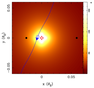
Figure 5: The geometry of the primary lens, source trajectory, caustics on the magnification map for the best 2L1S + xallarap model. The black filled circle on the left indicates the primary lens. The black filled circle on the right indicates the lens companion. The blue line with arrow represents the source trajectory. The blue circles represent the source size and position at $t_{0}$. The red closed curve represents the caustic. The colored contours represent the magnification map.

Table 11: Parameters of the 2L1S + xallarap + paralax + lens orbital motion models

Parameters	$q\leq 0.005$	$0.005<q\leq 0.01$	$0.01<q\leq 0.5$	$0.5<q\leq 1$
$t_{0}$(HJD-2458660)	$2.654\pm 0.016$	$2.592\pm 0.006$	$2.565\pm 0.003$	$2.578\pm 0.008$
$t_{\rm E}$ (days)	$98.1\pm 1.6$	$106.7\pm 1.4$	$109.2\pm 3.5$ $u_{0}$ ($10^{-3}$)	$-7.29\pm 0.18$	$-7.08\pm 0.07$	$-6.42\pm 0.21$	$6.43\pm 0.17$
$q$ ($10^{-2}$)	$3.14\pm 0.34$	$7.05\pm 0.17$	$47.2\pm 1.7$	$56.1\pm 5.2$
$s$	$0.222\pm 0.007$	$0.156\pm 0.002$	$0.080\pm 0.002$	$0.077\pm 0.002$
$\alpha$ (radian)	$0.359\pm 0.017$	$0.359\pm 0.087$	$1.887\pm 0.006$	$4.413\pm 0.014$
$\rho$ ($10^{-3}$)	$2.27\pm 0.15$	$2.21\pm 0.11$	$1.90\pm 0.11$	$1.93\pm 0.10$
$\pi_{{\rm E},N}$ ($10^{-1}$)	$2.43\pm 0.59$	$-0.25\pm 0.21$	$2.86\pm 0.40$	$2.76\pm 0.68$
$\pi_{{\rm E},E}$ ($10^{-1}$)	$1.08\pm 0.51$	$-0.29\pm 0.27$	$-1.95\pm 0.35$	$-1.52\pm 0.73$
${\rm R.A.}_{\xi}$ (degree)	$86.2\pm 11.1$	$50.1\pm 2.2$	$63.6\pm 3.0$	$82.2\pm 10.9$
${\rm decl.}_{\xi}$ (degree)	$28.0\pm 3.8$	$38.5\pm 1.3$	$71.9\pm 11.8$	$-42.5\pm 6.4$
$P_{\xi}$ (days)	$5.47\pm 0.04$	$5.46\pm 0.04$	$5.51\pm 0.04$	$5.53\pm 0.05$
$e_{\xi}$ ($10^{-1}$)	$1.94\pm 0.13$	$2.07\pm 0.30$	$1.37\pm 0.25$	$1.52\pm 0.29$
$T_{\rm peri}$ (HJD-2458600)	$62.56\pm 0.15$	$56.61\pm 0.05$	$63.31\pm 0.08$	$51.90\pm 0.20$
$\xi_{{\rm E},N}$ ($10^{-3}$)	$-2.87\pm 0.20$	$2.36\pm 0.09$	$0.93\pm 0.18$	$-1.34\pm 0.15$
$\xi_{{\rm E},E}$ ($10^{-3}$)	$1.25\pm 0.09$	$0.84\pm 0.09$	$1.21\pm 0.08$	$1.24\pm 0.21$
${d\alpha}/{dt}$ ($10^{-2}$ ${\rm radian}$ ${\rm yr}^{-1}$)	$-0.10\pm 0.05$	$0.50\pm 0.04$	$2.03\pm 0.16$	$-2.00\pm 0.12$
${ds}/{dt}$ ($10^{-2}$ ${\rm yr}^{-1}$)	$0.32\pm 0.01$	$1.39\pm 0.02$	$1.04\pm 0.03$	$0.94\pm 0.08$
$\chi^{2}$	10750.5	10746.1	10716.1	10742.4
$\Delta\chi^{2}$	34.6	30.1	-	26.4

Table 12: Comparisons between each microlensing model

Model	$N_{\rm param}$	$\chi^{2}$	$\Delta\chi^{2}$
1L1S	4	33144.7	22303.8
1L1S + xallarap	9	11311.5	470.6
1L1S + xallarap + parallax	11	11285.7	444.8
standard 2L1S	7	11744.7	903.7
2L1S + parallax	9	11676.5	835.5
2L1S + xallarap	12	10840.9	-

Table 13: Comparisons between Each Microlensing Models

Model	$N_{\rm param}$	$\chi^{2}$	$\Delta\chi^{2}$
1L1S	4	33144.7	22320.0
1L1S + xallarap	11	11184.2	359.5
standard 2L1S	7	11744.7	920.0
2L1S + parallax	9	11676.5	851.8
2L1S + xallarap	14	10824.7	-

4.4 Testing for higher order effects combinations

In a real binary lens event, whether detectable or not, the lens orbital motion and parallax effects should be present because both the lens companion and the Earth are orbiting their hosts. Therefore, we performed a fitting of the xallarap model with the parallax and lens orbital motion effects.

In addition, since the parallax and lens orbital motion effects are degenerate (Batista+2011; Skowron+2011; Bachelet+2012; Park+2013), the parallax effect must also be considered simultaneously when considering lens orbital motion. Simplified lens orbital motion effects can be modeled by adding the rate of change of the distance between lens components projected onto the lens plane at $t_{0}$, $ds/dt$ ; and the angular velocity relative to the source orbit, $d\alpha/dt$ (Batista+2011; Skowron+2011). The ratio of kinetic energy to potential energy projected onto the lensing plane of the lens companion can be written as follows (Dong et al., 2009; Skowron+2011):

$${\Bigm{|}\frac{\rm KE}{\rm PE}\Bigm{|}}_{\perp}={\frac{({a_{{\rm L},\perp}/{\rm au}})^{3}}{8\pi^{2}(M_{\rm L}/M_{\odot})}}\Bigm{[}\bigm{(}\frac{1}{s}\frac{ds}{dt}\bigm{)}^{2}+\frac{d\alpha}{dt}\Bigm{]},$$ (5)

where $M_{\rm L}$ is the total mass of the lensing system, and $a_{\perp}$ is the semi-major axis of the lensing companion star projected onto the lensing plane. $a_{{\rm L},\perp}$ can be described as $a_{{\rm L},\perp}=sD_{\rm L}\theta_{\rm E}$ using the distance $D_{\rm L}$ between the earth and the lens system, by

$$D_{\rm L}=\frac{\rm au}{\pi_{\rm E}\theta_{\rm E}+\pi_{\rm S}},$$ (6)

where $\pi_{\rm S}$ is the parallax of the source star, which can be written as $\pi_{\rm S}={\rm au}/D_{\rm S}$ using the distance $D_{\rm S}$ from the Earth to the source system. Following Miyazaki et al. (2020), we assumed $D_{\rm S}=8$ kpc in the sense that the source is in the Galactic bulge, and restricted the modeling to have $|{\rm KE}/{\rm PE}|_{\perp}<1$.

Furthermore, we found that the 2L1S + xallarap models with $\Delta\chi^{2}\leq 9$ from the best 2L1S + xallarap model in Section 4.3 have $50<t_{\rm E}$ [days]$<135$, $0.06<\theta_{\rm E}$ [mas] $<0.41$ and $0.35<\mu_{\rm{rel}}$ [$\rm{mas/yr}$] $<1.2$. We calculated the prior $\bm{\pi_{\rm{E}}}$ distribution of events with those parameters using the Galactic model by Koshimoto+2021b. To remove events that have too large $\pi_{\rm{E}}$ values, we limit the fitting range in the 2 $\sigma$ limit of the prior distribution of $0.024\leq\pi_{\rm{E}}\leq 0.351$.

The analysis of 2L1S + xallarap + parallax + lens orbital motion shows that various models exist in the parameter space of $s<1$, $0.01\lesssim q\lesssim 1$. The best 2L1S + xallarap + parallax + lens orbital motion model improved $\chi^{2}$ by $108.7$ from the 2L1S + xallarap model. However, from the cumulative $\Delta\chi^{2}$ in each data set for the 2L1S + xallarap + parallax + lens orbital motion model and the 2L1S + xallarap model, the $\chi^{2}$ improvement for the 2L1S + xallarap + parallax + lens orbital motion model is not consistent across data sets. Furthermore, the $\Delta\chi^{2}$ improvement is also highly influenced by the baseline systematic trend. This is the same as the case of the 2L1S + parallax model described in Section 4.2. We therefore conclude that the additional parallax + lens orbital motion signal is questionable. For the same reason, the 2L1S + xallarap + parallax model is also unreliable.

5 Source System Properties

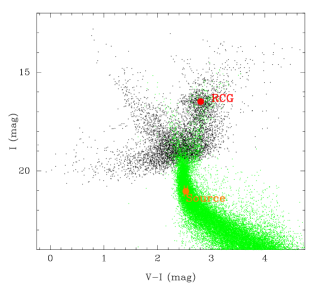
Figure 6: Color Magnitude Diagram (CMD, black dots) of the OGLE-$\mathrm{I}\mathrm{I}\mathrm{I}$ stars within $2’$ around OGLE-2019-BLG-0825. The green dots are stars in Baade’s window based on Hubble Space Telescope observations (Holtzman et al., 1998), color- and magnitude-matched at the RCG position. The orange circles represent the positions of the source, and the red dots represent the positions of the RCG centroid within $2’$ around OGLE-2019-BLG-0825.

We estimate the angular radius of the source host $\theta_{*}$ from the color and magnitude of the source. The apparent magnitude of the source, $R_{\rm MOA}$ and $V_{\rm MOA}$, are obtained from the modeling described in Section 4. However, the two bands have been scaled to match the instrumental MOA-$\mathrm{I}\mathrm{I}$ DOPHOT catalog (Bond+2017). Therefore, we converted them to Cousins $I$-band and Johnson $V-$band magnitude, using the OGLE-$\mathrm{I}\mathrm{I}\mathrm{I}$ catalog (Szymański et al., 2011). First, we cross-referenced the OGLE-$\mathrm{I}\mathrm{I}\mathrm{I}$ and the MOA catalogs. For stars within $2^{\prime}$ of the source star, we matched objects with the MOA-$\mathrm{I}\mathrm{I}$ DOPHOT catalog and the OGLE-$\mathrm{I}\mathrm{I}\mathrm{I}$ catalog coordinates within $0".7$. We estimated the angular source radius, $\theta_{*}$, from the color and magnitude of the source. The best fit instrumental source magnitudes of $R_{\rm MOA}$ and $V_{\rm MOA}$ are calibrated to the Cousins $I$-band and Johnson $V$-band magnitude scales by cross-referencing to the stars in the OGLE-$\mathrm{I}\mathrm{I}\mathrm{I}$ photometry map (Szymański et al., 2011) within $0\farcs 7$ of the event.

For reliability, we restricted stars to $16\leq V_{\rm OGLE-\mathrm{I}\mathrm{I}\mathrm{I}}$ [mag] $\leq 19$, and performed $5\sigma$ clipping in the linear regressions of $V_{\rm MOA}$ vs. $V_{\rm OGLE-\mathrm{I}\mathrm{I}\mathrm{I}}$ and $(I_{\rm OGLE-\mathrm{I}\mathrm{I}\mathrm{I}}-R_{\rm MOA})$ vs. $(V-R)_{\rm MOA}$ and $(V-I)_{\rm OGLE-\mathrm{I}\mathrm{I}\mathrm{I}}$ vs. $(V-R)_{\rm MOA}$, respectively. From the final 73 remaining objects, the following conversion equations from $R_{\rm MOA}$ and $(V-R)_{\rm MOA}$ to $I_{\rm OGLE-\mathrm{I}\mathrm{I}\mathrm{I}}$ and $(V-I)_{\rm OGLE-\mathrm{I}\mathrm{I}\mathrm{I}}$ were obtained by linear regression,

$$I_{\rm OGLE-\mathrm{I}\mathrm{I}\mathrm{I}}=R_{\rm MOA}-(0.24\pm 0.01)\times(V-R)_{\rm MOA}+(27.22\pm 0.01),$$ (7)

$$(V-I)_{\rm OGLE-\mathrm{I}\mathrm{I}\mathrm{I}}=(1.20\pm 0.01)\times(V-R)_{\rm MOA}+(0.94\pm 0.02).$$ (8)

As a result, the color and magnitude with the extinction of the source star for the best fit 2L1S + xallarap model was $(V-I,I)_{\rm S}=(2.527\pm 0.031,$ $21.035\pm 0.015)$. The intrinsic color and magnitude of RCG stars are $(V-I,I)_{{\rm RCG},0}=(1.060\pm 0.060,$ $14.443\pm 0.040)$ (Bensby et al., 2013; Nataf et al., 2013). From the color-magnitude diagram of the stars within $2^{\prime}$ of the source star (Figure 6), the RCG centroid is estimated as $(V-I,I)_{\rm RCG}=(2.804\pm 0.009,$ $16.488\pm 0.022)$. Then we calculated $(E(V-I),A(I))=(1.744\pm 0.061,$ $2.045\pm 0.046)$. Finally, we have the intrinsic color and magnitude of the source star $(V-I,I)_{\rm S,0}=(0.783\pm 0.068,$ $18.990\pm 0.048)$ for the best 2L1S + xallarap model. Also, Figure 6 shows that the source is a main-sequence star and unlikely to be a variable star. Table 16 shows that the values for $(V-I,I)_{\rm S,0}$ for the other models are almost the same.

Boyajian et al. (2014) derived the following relationship between the apparent radius $\theta_{*}$ and color magnitude from nearby main-sequence stars,

$$\log(2\theta_{*})=0.50+0.42(V-I)_{0}-0.2I_{0}.$$ (9)

This relationship comes from private communication with them, which is limited to FGK stars with $3900$ $<T_{\rm{eff}}$ [K] $<7000$, and the accuracy of the relational equation is better than $2\%$ (Fukui et al., 2015). We estimated the angular source radius $\theta_{*}=0.568\pm 0.039$ $\mu$as from the Equation (10).

We estimated the angular source radius of $\theta_{*}=0.538\pm 0.039$ $\mu$as from the relation,

$$\log(2\theta_{*})=0.50+0.42(V-I)_{0}-0.2I_{0},$$ (10)

where the accuracy of the relational equation is better than 2% (Fukui et al., 2015). This relation is based on Boyajian et al. (2014), but derived by limiting to FGK stars with $3900$ $<T_{\rm{eff}}$ [K] $<7000$ (Boyajian, 2014, Private Communication). Then, we calculated the lens’s Einstein radius of $\theta_{\rm E}=\rho\theta_{*}=0.25\pm 0.02$ mas and the lens-source relative proper motion of $\mu_{\rm rel}=\theta_{\rm E}/t_{\rm E}=0.97\pm 0.10$ mas $\rm{yr^{-1}}$.

The amplitude of the xallarap vector, $\xi_{\rm E}$ is described as follows,

$$\xi_{\rm E}\equiv\Bigl{(}\frac{\theta_{\rm E}D_{\rm S}}{1\>\rm{au}}\Bigr{)}^{-1}\Bigl{(}\frac{P_{\xi}}{1\>\rm{yr}}\Bigr{)}^{2/3}\Bigl{(}\frac{M_{\rm S,C}}{M_{\odot}}\Bigr{)}\Bigl{(}\frac{M_{\rm S,H}+M_{\rm S,C}}{M_{\odot}}\Bigr{)}^{-2/3},$$ (11)

where $M_{\rm S,H}$ and $M_{\rm S,C}$ are the masses of host and companion of the source system, respectively. $M_{\rm S,H}$ is estimated by using isochrones (PARSEC; Bressan et al., 2012) and the absolute magnitude of the host source star $M(I_{\rm S})=I_{\rm{S,0}}+5\log_{10}{D_{\rm S}{\rm{[pc]}}}+5=4.48\pm 0.38$ mag assuming $D_{\rm S}=8.0\pm 1.4$ kpc. Then, $M_{\rm S,C}$ can be solved from Equation (11). Also, using Kepler’s third law,

$$\Bigl{(}\frac{a_{\rm S}}{1\>\rm{au}}\Bigr{)}^{3}\Bigl{(}\frac{P_{\xi}}{1\>\rm{yr}}\Bigr{)}^{-2}=\Bigl{[}\frac{M_{\rm S,H}+M_{\rm S,C}}{M_{\odot}}\Bigr{]},$$ (12)

we can solve $a_{\rm S}$ which is the semi-major axis of the source system. The apparent $H$- and $K$-bands magnitudes of the source with extinction $H_{\rm S}$ and $K_{\rm S}$ are also estimated using PARSEC isochrones and the wavelength dependence of the extinction law in the direction of Galactic center, $A_{V}:A_{H}:A_{K_{s}}=1:0.108:0.062$ (Nishiyama et al., 2008). In addition, we calculated $L_{\rm S,C}/L_{\rm S,H}$, the luminosity ratio in the $I$-band of the source companion $L_{\rm S,C}$ to the source host $L_{\rm S,H}$. For this we used the mass-luminosity empirical relation of Bennett et al. (2015), which combines Henry & McCarthy (1993) and Delfosse et al. (2000), and the isochrone model of Baraffe et al. (2003). We used the Henry & McCarthy (1993) relation for $M>0.66$ $M_{\odot}$, the Delfosse et al. (2000) relation for $0.12$ $M_{\odot}<M<0.54$ $M_{\odot}$. For low-mass stars ($M<0.10$ $M_{\odot}$) we used the isochrone model of Baraffe et al. (2003) for sub-stellar objects at an age of 10 Gyr. At the boundary of these mass ranges, we interpolated linearly between the two relations. Table 16 shows our calculated properties of the source system for the 2L1S + xallarap models in Table 6. The source host in the best 2L1S + xallarap model is a G-type main-sequence star and the source companion is a brown dwarf with a semi major axis of $a_{\rm S}=0.0594\pm 0.0005$ au. The luminosity ratio at the $I$-band of the source companion $L_{\rm S,C}$ is small, $L_{\rm S,C}/L_{\rm S,H}=(1.0\pm 0.3)\times 10^{-7}$, and does not conflict with our assumption the magnified flux of the second source is too weak to be detected.

Table 14: Source system properties of the 2L1S + xallarap models

Model	XLclose1	XLclose2	XLwide1	XLwide2
range of $q$	$q\leq 0.1$	$0.1<q\leq 1$	$q\leq 0.1$	$0.1<q\leq 1$
$V_{\rm S}$ (mag)	$23.58\pm 0.03$	$23.56\pm 0.03$	$23.55\pm 0.03$	$23.56\pm 0.03$
$I_{\rm S}$ (mag)	$21.06\pm 0.01$	$21.04\pm 0.01$	$21.02\pm 0.01$	$21.06\pm 0.01$
$H_{\rm S}$ (mag)	$18.54\pm 0.30$	$18.52\pm 0.484$	$18.51\pm 0.48$	$18.54\pm 0.48$
$K_{\rm S}$ (mag)	$18.31\pm 0.48$	$18.29\pm 0.48$	$18.28\pm 0.48$	$18.31\pm 0.48$
$(V-I)_{\rm S}$ (mag)	$2.52\pm 0.03$	$2.53\pm 0.03$	$2.52\pm 0.03$	$2.527\pm 0.03$
$I_{\rm S,0}$ (mag)	$19.01\pm 0.05$	$18.99\pm 0.05$	$19.00\pm 0.05$	$19.01\pm 0.05$
$(V-I)_{\rm S,0}$ (mag)	$0.78\pm 0.07$	$0.78\pm 0.07$	$0.78\pm 0.07$	$0.78\pm 0.07$
$M_{I}$ (mag)	$4.50\pm 0.38$	$4.48\pm 0.38$	$4.46\pm 0.38$	$4.50\pm 0.38$
$\theta_{\rm E}$ (mas)	$0.53\pm 0.04$	$0.25\pm 0.02$	$0.22\pm 0.02$	$0.37\pm 0.05$
$\mu_{\rm rel}$ (mas ${\rm yr}^{-1}$)	$0.78\pm 0.07$	$0.97\pm 0.10$	$0.81\pm 0.07$	$1.01\pm 0.16$
$M_{\rm S,H}$ ($M_{\odot}$)	$0.864\pm 0.045$	$0.867\pm 0.045$	$0.868\pm 0.045$	$0.864\pm 0.045$
$M_{\rm S,C}$ ($M_{\odot}$)	$0.050\pm 0.005$	$0.048\pm 0.004$	$0.047\pm 0.004$	$0.051\pm 0.006$
$a_{\rm S}$ ($10^{-2}$ au)	$5.86\pm 0.04$	$5.94\pm 0.05$	$5.87\pm 0.03$	$5.95\pm 0.05$
$L_{\rm S,C}/L_{\rm S,H}$ ($10^{-7}$)	$1.15\pm 0.34$	$1.02\pm 0.26$	$0.95\pm 0.23$	$1.21\pm 0.47$
$\chi^{2}$	10856.4	10840.9	10861.2	10842.7
$\Delta\chi^{2}$	15.5	-	20.3	1.8

Table 15: Source system properties of the 2L1S + xallarap models

Model	XLclose1	XLclose2	XLwide1	XLwide2
range of $q$	$q\leq 0.1$	$0.1<q\leq 1$	$q\leq 0.1$	$0.1<q\leq 1$
$V_{\rm S}$ (mag)	$23.581\pm 0.034$	$23.562\pm 0.034$	$23.545\pm 0.034$	$23.564\pm 0.034$
$I_{\rm S}$ (mag)	$21.057\pm 0.015$	$21.035\pm 0.015$	$21.022\pm 0.015$	$21.057\pm 0.015$
$H_{\rm S}$ (mag)	$18.538\pm 0.300$	$18.521\pm 0.485$	$18.511\pm 0.484$	$18.538\pm 0.484$
$K_{\rm S}$ (mag)	$18.308\pm 0.478$	$18.293\pm 0.479$	$18.282\pm 0.479$	$18.308\pm 0.479$
$(V-I)_{\rm S}$ (mag)	$2.524\pm 0.031$	$2.527\pm 0.031$	$2.523\pm 0.031$	$2.527\pm 0.031$
$I_{\rm S,0}$ (mag)	$19.012\pm 0.048$	$18.990\pm 0.048$	$18.997\pm 0.048$	$19.012\pm 0.048$
$(V-I)_{\rm S,0}$ (mag)	$0.780\pm 0.068$	$0.783\pm 0.068$	$0.779\pm 0.068$	$0.783\pm 0.068$
$M_{I}$ (mag)	$4.496\pm 0.384$	$4.476\pm 0.384$	$4.462\pm 0.384$	$4.496\pm 0.384$
$\theta_{\rm E}$ (mas)	$0.531\pm 0.038$	$0.250\pm 0.023$	$0.224\pm 0.019$	$0.369\pm 0.048$
$\mu_{\rm rel}$ (mas ${\rm yr}^{-1}$)	$0.775\pm 0.072$	$0.973\pm 0.096$	$0.812\pm 0.073$	$1.012\pm 0.158$
$M_{\rm S,H}$ ($M_{\odot}$)	$0.864\pm 0.045$	$0.867\pm 0.045$	$0.868\pm 0.045$	$0.864\pm 0.045$
$M_{\rm S,C}$ ($M_{\odot}$)	$0.050\pm 0.005$	$0.048\pm 0.004$	$0.047\pm 0.004$	$0.051\pm 0.006$
$a_{\rm S}$ ($10^{-2}$ au)	$5.859\pm 0.040$	$5.942\pm 0.047$	$5.874\pm 0.033$	$5.948\pm 0.047$
$L_{\rm S,C}/L_{\rm S,H}$ ($10^{-7}$)	$1.154\pm 0.339$	$1.019\pm 0.264$	$0.953\pm 0.230$	$1.205\pm 0.472$
$\chi^{2}$	10856.4	10840.9	10861.2	10842.7
$\Delta\chi^{2}$	15.5	-	20.3	1.8

20230528 $V_{\rm S}$ (mag) & $19.791\pm 0.083$ $\pm$ $\pm$ $\pm$
$I_{\rm S}$ (mag) $21.057\pm 0.015$ $21.035\pm 0.015$ $21.022\pm 0.015$ $21.057\pm 0.015$
$H_{\rm S}$ (mag) $\pm$ $\pm$ $\pm$ $\pm$
$K_{\rm S}$ (mag) $\pm$ $\pm$ $\pm$ $\pm$
$(V-I)_{\rm S}$ (mag) $2.524\pm 0.031$ $2.527\pm 0.031$ $2.523\pm 0.031$ $2.527\pm 0.031$
$I_{\rm S,0}$ (mag) $19.012\pm 0.048$ $18.990\pm 0.048$ $18.997\pm 0.048$ $19.012\pm 0.048$
$(V-I)_{\rm S,0}$ (mag) $0.780\pm 0.068$ $0.783\pm 0.068$ $0.779\pm 0.068$ $0.783\pm 0.068$
$M_{I}$ (mag) $4.496\pm 0.384$ $4.476\pm 0.384$ $4.462\pm 0.384$ $4.496\pm 0.384$
$\theta_{\rm E}$ (mas) $0.531\pm 0.038$ $0.250\pm 0.023$ $0.224\pm 0.019$ $0.369\pm 0.048$
$\mu_{\rm rel}$ (mas ${\rm yr}^{-1}$) $0.775\pm 0.072$ $0.973\pm 0.096$ $0.812\pm 0.073$ $1.012\pm 0.158$
$M_{\rm S,H}$ ($M_{\odot}$) $0.865\pm 0.045$ $0.867\pm 0.045$ $0.869\pm 0.045$ $0.865\pm 0.045$
$M_{\rm S,C}$ ($M_{\odot}$) $0.050\pm 0.005$ $0.048\pm 0.004$ $0.047\pm 0.004$ $0.051\pm 0.006$
$a_{\rm S}$ ($10^{-2}$ au) $5.860\pm 0.043$ $5.943\pm 0.051$ $5.874\pm 0.033$ $5.949\pm 0.051$
$L_{\rm S,C}/L_{\rm S,H}$ ($10^{-7}$) $1.155\pm 0.340$ $1.019\pm 0.264$ $0.954\pm 0.230$ $1.206\pm 0.472$

Table 16: Source system properties of the 2L1S + xallarap models

Model	XLclose1	XLclose2	XLclose3	XLwide1	XLwide2	XLwide3
range of $q$	$q\leq 0.1$	$0.1<q\leq 0.5$	$0.5<q\leq 1$	$q\leq 0.1$	$0.1<q\leq 0.5$	$0.5<q\leq 1$
$I_{\rm s,0}$ (mag)	$19.012\pm 0.048$	$18.990\pm 0.048$	$19.008\pm 0.048$	$18.997\pm 0.048$	$19.014\pm 0.048$	$19.012\pm 0.048$
$(V-I)_{\rm s,0}$ (mag)	$0.780\pm 0.068$	$0.783\pm 0.068$	$0.782\pm 0.068$	$0.779\pm 0.068$	$0.782\pm 0.068$	$0.783\pm 0.068$
$\theta_{\rm E}$ (mas)	$0.531\pm 0.038$	$0.250\pm 0.023$	$0.252\pm 0.026$	$0.224\pm 0.019$	$0.309\pm 0.030$	$0.369\pm 0.048$
$\mu_{\rm rel}$ (mas ${\rm yr}^{-1}$)	$0.775\pm 0.072$	$0.973\pm 0.096$	$0.963\pm 0.102$	$0.812\pm 0.073$	$0.976\pm 0.104$	$1.012\pm 0.158$
$M_{\rm S,H}$ ($M_{\odot}$)	$0.865\pm 0.045$	$0.867\pm 0.045$	$0.865\pm 0.045$	$0.869\pm 0.045$	$0.864\pm 0.045$	$0.865\pm 0.045$
$M_{\rm S,C}$ ($M_{\odot}$)	$0.050\pm 0.005$	$0.048\pm 0.004$	$0.048\pm 0.006$	$0.047\pm 0.004$	$0.050\pm 0.004$	$0.051\pm 0.006$
$a_{\rm S}$ ($10^{-2}$ au)	$5.860\pm 0.043$	$5.943\pm 0.051$	$5.952\pm 0.055$	$5.874\pm 0.033$	$5.932\pm 0.054$	$5.949\pm 0.051$
$L_{\rm S,C}/L_{\rm S,H}$ ($10^{-7}$)	$1.155\pm 0.340$	$1.019\pm 0.264$	$1.003\pm 0.393$	$0.954\pm 0.230$	$1.122\pm 0.297$	$1.206\pm 0.472$
$\chi^{2}$	10856.4	10840.9	10842.3	10861.2	10843.4	10842.7
$\Delta\chi^{2}$	15.5	-	1.3	20.3	2.4	1.8

Table 17: Source system properties of the 2L1S + xallarap wide models

Model	XLwide1	XLwide2	XLwide3	XLwide4
range of $q$	$q\leq 0.001$	$0.001<q\leq 0.01$	$0.01<q\leq 0.1$	$0.1<q\leq 1$
$I_{\rm s,0}$ (mag)	$18.831\pm 0.048$	$18.986\pm 0.048$	$19.011\pm 0.048$	$19.014\pm 0.048$
$(V-I)_{\rm s,0}$ (mag)	$0.777\pm 0.068$	$0.780\pm 0.068$	$0.780\pm 0.068$	$0.781\pm 0.068$
$\theta_{\rm E}$ (mas)	$0.061\pm 0.004$	$0.124\pm 0.010$	$0.236\pm 0.024$	$0.256\pm 0.027$
$\mu_{\rm rel}$ (mas ${\rm yr}^{-1}$)	$0.397\pm 0.029$	$0.421\pm 0.034$	$0.879\pm 0.091$	$0.892\pm 0.094$
$M_{\rm S,H}$ ($M_{\odot}$)	$0.861\pm 0.047$	$0.868\pm 0.045$	$0.865\pm 0.045$	$0.864\pm 0.045$
$M_{\rm S,C}$ ($M_{\odot}$)	$0.036\pm 0.001$	$0.071\pm 0.004$	$0.104\pm 0.012$	$0.064\pm 0.005$
$a_{\rm S}$ ($10^{-2}$ au)	$5.305\pm 0.029$	$5.885\pm 0.040$	$5.960\pm 0.056$	$5.957\pm 0.051$
$L_{\rm S,C}/L_{\rm S,H}$ ($10^{-4}$)	$0.001\pm 0.001$	$0.010\pm 0.045$	$1.514\pm 0.535$	$0.004\pm 0.010$
$\chi^{2}$	10829.1	10831.6	10824.7	10830.5
$\Delta\chi^{2}$	4.4	6.9	-	5.8

Table 18: Source system properties of the 2L1S + xallarap close models

Model	XLclose1	XLclose2	XLclose3	XLclose4
range of $q$	$q\leq 0.001$	$0.001<q\leq 0.01$	$0.1<q\leq 0.5$	$0.1<q\leq 1$
$I_{\rm s,0}$ (mag)	$19.027\pm 0.048$	$18.954\pm 0.048$	$18.990\pm 0.048$	$19.011\pm 0.048$
$(V-I)_{\rm s,0}$ (mag)	$0.779\pm 0.068$	$0.782\pm 0.068$	$0.783\pm 0.068$	$0.781\pm 0.068$
$\theta_{\rm E}$ (mas)	$0.479\pm 0.204$	$0.124\pm 0.012$	$0.250\pm 0.024$	$0.240\pm 0.024$
$\mu_{\rm rel}$ (mas ${\rm yr}^{-1}$)	$2.105\pm 0.897$	$0.636\pm 0.062$	$0.973\pm 0.099$	$0.891\pm 0.094$
$M_{\rm S,H}$ ($M_{\odot}$)	$0.863\pm 0.047$	$0.871\pm 0.045$	$0.867\pm 0.045$	$0.865\pm 0.045$
$M_{\rm S,C}$ ($M_{\odot}$)	$0.172\pm 0.060$	$0.072\pm 0.005$	$0.048\pm 0.005$	$0.067\pm 0.009$
$a_{\rm S}$ ($10^{-2}$ au)	$6.150\pm 0.128$	$5.880\pm 0.044$	$5.943\pm 0.058$	$5.953\pm 0.055$
$L_{\rm S,C}/L_{\rm S,H}$ ($10^{-7}$)	$5.573\pm 4.514$	$0.018\pm 0.024$	$1.019\pm 0.381$	$0.004\pm 0.047$
$\chi^{2}$	10836.8	10831.4	10842.5	10830.7
$\Delta\chi^{2}$	12.2	6.8	-	6.0

Table 19: Source system properties of the 2L1S + xallarap wide models

Model	XLwide1	XLwide2	XLwide3	XLwide4
range of $q$	$q\leq 0.001$	$0.001<q\leq 0.01$	$0.01<q\leq 0.1$	$0.1<q\leq 1$
$I_{\rm s,0}$ (mag)	$18.831\pm 0.048$	$18.986\pm 0.048$	$19.011\pm 0.048$	$19.014\pm 0.048$
$(V-I)_{\rm s,0}$ (mag)	$0.777\pm 0.068$	$0.780\pm 0.068$	$0.780\pm 0.068$	$0.781\pm 0.068$
$\theta_{\rm E}$ (mas)	$0.061\pm 0.004$	$0.124\pm 0.010$	$0.236\pm 0.024$	$0.256\pm 0.027$
$\mu_{\rm rel}$ (mas ${\rm yr}^{-1}$)	$0.397\pm 0.029$	$0.421\pm 0.034$	$0.879\pm 0.091$	$0.892\pm 0.094$
$M_{\rm S,H}$ ($M_{\odot}$)	$0.861\pm 0.047$	$0.868\pm 0.045$	$0.865\pm 0.045$	$0.864\pm 0.045$
$M_{\rm S,C}$ ($M_{\odot}$)	$0.036\pm 0.001$	$0.071\pm 0.004$	$0.104\pm 0.012$	$0.064\pm 0.005$
$a_{\rm S}$ ($10^{-2}$ au)	$5.305\pm 0.029$	$5.885\pm 0.040$	$5.960\pm 0.056$	$5.957\pm 0.051$
$L_{\rm S,C}/L_{\rm S,H}$ ($10^{-4}$)	$0.001\pm 0.001$	$0.010\pm 0.045$	$1.514\pm 0.535$	$0.004\pm 0.010$
$\chi^{2}$	10829.1	10831.6	10824.7	10830.5
$\Delta\chi^{2}$	4.4	6.9	-	5.8

Table 20: Source system properties of the 2L1S + xallarap close models

Model	XLclose1	XLclose2	XLclose3	XLclose4
range of $q$	$q\leq 0.001$	$0.001<q\leq 0.01$	$0.01<q\leq 0.1$	$0.1<q\leq 1$
$I_{\rm s,0}$ (mag)	$19.027\pm 0.048$	$18.954\pm 0.048$	$19.005\pm 0.048$	$19.011\pm 0.048$
$(V-I)_{\rm s,0}$ (mag)	$0.779\pm 0.068$	$0.782\pm 0.068$	$0.781\pm 0.068$	$0.781\pm 0.068$
$\theta_{\rm E}$ (mas)	$0.479\pm 0.204$	$0.124\pm 0.012$	$0.231\pm 0.024$	$0.240\pm 0.024$
$\mu_{\rm rel}$ (mas ${\rm yr}^{-1}$)	$2.105\pm 0.897$	$0.636\pm 0.062$	$0.878\pm 0.095$	$0.891\pm 0.094$
$M_{\rm S,H}$ ($M_{\odot}$)	$0.863\pm 0.047$	$0.871\pm 0.045$	$0.865\pm 0.045$	$0.865\pm 0.045$
$M_{\rm S,C}$ ($M_{\odot}$)	$0.172\pm 0.060$	$0.072\pm 0.005$	$0.102\pm 0.009$	$0.067\pm 0.009$
$a_{\rm S}$ ($10^{-2}$ au)	$6.150\pm 0.128$	$5.880\pm 0.044$	$5.983\pm 0.043$	$5.953\pm 0.055$
$L_{\rm S,C}/L_{\rm S,H}$ ($10^{-4}$)	$5.573\pm 4.514$	$0.018\pm 0.024$	$1.451\pm 0.393$	$0.004\pm 0.047$
$\chi^{2}$	10836.8	10831.4	10825.3	10830.7
$\Delta\chi^{2}$	12.2	6.8	0.6	6.0

The distance from the Earth to the lensing system $D_{\rm L}$ can be described by Equation 17, and the total mass of the host and companion in the lensing system $M_{\rm L}$ can be described by the following equation (Gaudi, 2012),

$$M_{\rm L}=\frac{\theta_{\rm E}}{\kappa\pi_{\rm E}},$$ (13)

where $\kappa=4G/(c^{2}{\rm au})\sim 8.144$ [mas $M_{\odot}^{-1}$]. The host mass of the lens system $M_{\rm L,H}$ and companion mass $M_{\rm L,C}$ of the lens system and their projection semi-major distance to the lensing plane $a_{{\rm L},\perp}$ can be expressed by the following equations, respectively,

$$M_{\rm L,H}=\frac{M_{\rm L}}{1+q},$$ (14)

$$M_{\rm L,C}=\frac{qM_{\rm L}}{1+q},$$ (15)

$$a_{{\rm L},\perp}=s\theta_{\rm E}D_{\rm L},$$ (16)

The expected value of the semi-major distance of lens companion in three dimensions can be expressed by $a_{\rm L,exp}=\sqrt{3/2}a_{\rm L,\perp}$. We calculated $a_{\rm L,exp}/a_{\rm snow}$, which is the value of $a_{\rm L,exp}$ normalized by the snow line position $a_{\rm snow}=2.7(M_{\rm H}/M_{\odot})$. Table 21 shows the properties of the source and lens systems calculated for the 2L1S xallarap + parallax + lens orbital motion models in Table 11. As can be seen from Table 21, the properties of the lens system have large uncertainties. This is due to the large uncertainties in the parallax and lens revolution parameters shown in Table 11. However, the source system properties are consistently the same as those of the 2L1S+xallarap models shown in Tables 19 and 20.

Table 21: Source system properties of the 2L1S + xallarap + parallax + lens orbital motion models

Parameters	$q\leq 0.05$	$0.005<q\leq 0.1$	$0.1<q\leq 0.5$	$0.5<q\leq 1$
$I_{\rm s,0}$ (mag)	$18.882\pm 0.026$	$18.919\pm 0.011$	$18.979\pm 0.036$	$18.976\pm 0.031$
$(V-I)_{\rm s,0}$ ($10^{-1}$ mag)	$7.829\pm 0.018$	$7.777\pm 0.018$	$7.806\pm 0.019$	$7.800\pm 0.018$
$\theta_{\rm E}$ (mas)	$0.249\pm 0.018$	$0.250\pm 0.013$	$0.284\pm 0.016$	$0.281\pm 0.018$
$\mu_{\rm rel}$ (mas ${\rm yr}^{-1}$)	$0.928\pm 0.067$	$0.857\pm 0.043$	$0.949\pm 0.065$	$0.946\pm 0.078$
$M_{\rm S,H}$ ($M_{\odot}$)	$0.880\pm 0.003$	$0.876\pm 0.001$	$0.868\pm 0.004$	$0.869\pm 0.004$
$M_{\rm S,C}$ ($M_{\odot}$)	$0.010\pm 0.001$	$0.080\pm 0.006$	$0.054\pm 0.005$	$0.064\pm 0.007$
$a_{\rm S}$ ($10^{-2}$ au)	$6.04\pm 0.03$	$5.98\pm 0.04$	$5.94\pm 0.03$	$5.98\pm 0.05$
$L_{\rm S,C}/L_{\rm S,H}$ ($10^{-3}$)	$1.01\pm 0.44$	$1.19\pm 0.21$	$0.49\pm 0.12$	$0.72\pm 0.20$
$D_{\rm L}$ (kpc)	$5.23\pm 0.36$	$7.43\pm 0.31$	$4.48\pm 0.32$	$4.69\pm 0.56$
$M_{\rm L,H}$ ($M_{\odot}$)	$0.112\pm 0.014$	$0.753\pm 0.356$	$0.068\pm 0.010$	$0.070\pm 0.016$
$M_{\rm L,C}$ ($10^{-2}$ $M_{\odot}$)	$0.35\pm 0.04$	$5.31\pm 2.47$	$3.23\pm 0.47$	$3.92\pm 0.96$
$a_{{\rm L},\perp}$ (au)	$0.29\pm 0.03$	$0.29\pm 0.02$	$0.10\pm 0.01$	$0.10\pm 0.01$
$a_{\rm L,exp}$ (au)	$0.35\pm 0.03$	$0.36\pm 0.03$	$0.12\pm 0.01$	$0.12\pm 0.01$
$a_{\rm L,exp}/a_{\rm snow}$	$1.17\pm 0.10$	$0.18\pm 0.09$	$0.68\pm 0.07$	$0.65\pm 0.10$
$\chi^{2}$	10750.5	10746.1	10716.1	10742.4
$\Delta\chi^{2}$	34.6	30.1	-	26.4

6 Lens System Properties by Bayesian Analysis

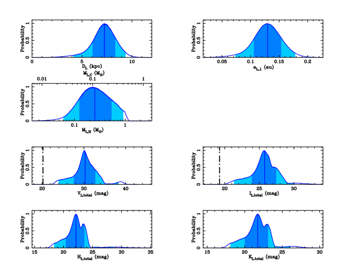
Figure 7: Posterior probability distribution of the properties of the lens system by Bayesian analysis for XLclose2. In each panel, the dark blue region indicates the $68.3\%$ credible interval, light blue region indicates the $95.4\%$ credible interval, and the blue vertical line indicates the median value. The dashed lines at the left end of the panel of apparent $V$- and $I$-band magnitudes with extinction are the blending magnitudes obtained from light curve modeling and are considered as the upper limit of brightness of the lens system.

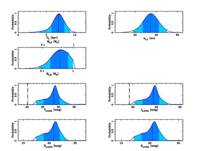
Figure 8: Same as Figure 7, but for XLwide2.

Table 22: Lens system properties of the 2L1S + xallarap models

Model	XLclose1	XLclose2	XLwide1	XLwide2
range of $q$	$q\leq 0.1$	$0.1<q\leq 1$	$q\leq 0.1$	$0.1<q\leq 1$
$D_{\rm L}$ (kpc)	$7.27_{-1.17}^{+1.10}$	$7.24_{-1.17}^{+1.09}$	$7.24_{-1.18}^{+1.09}$	$7.12_{-1.214}^{+1.05}$
$M_{\rm L,H}$ ($M_{\odot}$)	$0.23_{-0.12}^{+0.28}$	$0.25_{-0.13}^{+0.29}$	$0.26_{-0.13}^{+0.29}$	$0.37_{-0.19}^{+0.32}$
$M_{\rm L,C}$ ($M_{\odot}$)	$0.02_{-0.01}^{+0.03}$	$0.11_{-0.06}^{+0.13}$	$0.03_{-0.01}^{+0.03}$	$0.35_{-0.18}^{+0.30}$
$a_{\rm{L,\perp}}$ (au)	$0.20_{-0.04}^{+0.04}$	$0.13_{-0.02}^{+0.02}$	$11.55_{-2.09}^{+2.03}$	$34.74_{-7.69}^{+7.51}$
$a_{\rm L,exp}$ (au)	$0.25_{-0.06}^{+0.13}$	$0.16_{-0.04}^{+0.08}$	$13.91_{-3.15}^{+7.39}$	$42.10_{-10.92}^{+21.78}$
$V_{\rm L,H}$ (mag)	$30.61_{-2.54}^{+2.56}$	$30.34_{-2.66}^{+2.42}$	$30.25_{-2.71}^{+2.31}$	$29.17_{-3.38}^{+1.83}$
$I_{\rm L,H}$ (mag)	$26.09_{-1.75}^{+1.66}$	$25.90_{-1.83}^{+1.57}$	$25.84_{-1.86}^{+1.51}$	$25.05_{-2.35}^{+1.22}$
$H_{\rm L,H}$ (mag)	$22.53_{-1.73}^{+1.27}$	$22.35_{-1.80}^{+1.26}$	$22.30_{-1.82}^{+1.23}$	$21.53_{-2.02}^{+1.17}$
$K_{\rm L,H}$ (mag)	$22.11_{-1.70}^{+1.21}$	$21.93_{-1.75}^{+1.20}$	$21.87_{-1.77}^{+1.18}$	$21.12_{-1.94}^{+1.14}$
$V_{\rm L,C}$ (mag)	$41.53_{-1.76}^{+0.98}$	$33.68_{-2.97}^{+6.20}$	$41.42_{-2.13}^{+1.03}$	$29.35_{-3.13}^{+1.88}$
$I_{\rm L,C}$ (mag)	$35.24_{-3.05}^{+1.75}$	$28.13_{-1.94}^{+3.32}$	$34.85_{-3.13}^{+1.88}$	$25.18_{-2.16}^{+1.25}$
$H_{\rm L,C}$ (mag)	$33.74_{-3.99}^{+3.00}$	$24.12_{-1.50}^{+5.98}$	$33.42_{-4.24}^{+3.12}$	$21.66_{-1.92}^{+1.16}$
$K_{\rm L,C}$ (mag)	$30.45_{-2.24}^{+1.47}$	$23.63_{-1.44}^{+3.68}$	$30.00_{-2.24}^{+1.54}$	$21.25_{-1.85}^{+1.14}$
$V_{\rm L,total}$ (mag)	$30.60_{-2.54}^{+2.55}$	$30.29_{-2.68}^{+2.46}$	$30.25_{-2.71}^{+2.31}$	$28.50_{-3.27}^{+1.85}$
$I_{\rm L,total}$ (mag)	$26.08_{-1.75}^{+1.65}$	$25.77_{-1.86}^{+1.67}$	$25.83_{-1.86}^{+1.51}$	$24.36_{-2.26}^{+1.24}$
$H_{\rm L,total}$ (mag)	$22.53_{-1.73}^{+1.27}$	$22.16_{-1.76}^{+1.44}$	$22.30_{-1.82}^{+1.22}$	$20.84_{-1.98}^{+1.16}$
$K_{\rm L,total}$ (mag)	$22.10_{-1.70}^{+1.21}$	$21.73_{-1.71}^{+1.38}$	$21.87_{-1.77}^{+1.18}$	$20.43_{-1.89}^{+1.14}$
$V_{\rm Blend}$ (mag)	$20.21\pm 0.03$	$20.21\pm 0.03$	$20.21\pm 0.03$	$20.21\pm 0.03$
$I_{\rm Blend}$ (mag)	$19.25\pm 0.01$	$19.25\pm 0.01$	$19.25\pm 0.01$	$19.25\pm 0.01$
$\chi^{2}$	10856.4	10840.9	10861.2	10842.7
$\Delta\chi^{2}$	15.5	-	20.3	1.8

Table 23: Lens system properties of the 2L1S + xallarap models

Model	XLclose1	XLclose2	XLwide1	XLwide2
range of $q$	$q\leq 0.1$	$0.1<q\leq 1$	$q\leq 0.1$	$0.1<q\leq 1$
$D_{\rm L}$ (kpc)	$7.272_{-1.168}^{+1.098}$	$7.244_{-1.171}^{+1.087}$	$7.242_{-1.183}^{+1.091}$	$7.115_{-1.215}^{+1.047}$
$M_{\rm L,H}$ ($M_{\odot}$)	$0.232_{-0.117}^{+0.277}$	$0.253_{-0.128}^{+0.287}$	$0.261_{-0.131}^{+0.290}$	$0.373_{-0.190}^{+0.319}$
$M_{\rm L,C}$ ($M_{\odot}$)	$0.022_{-0.011}^{+0.026}$	$0.111_{-0.056}^{+0.126}$	$0.026_{-0.013}^{+0.029}$	$0.352_{-0.179}^{+0.301}$
$a_{\rm{L,\perp}}$ (au)	$0.205_{-0.037}^{+0.037}$	$0.130_{-0.024}^{+0.024}$	$11.549_{-2.087}^{+2.031}$	$34.741_{-7.691}^{+7.512}$
$a_{\rm L,exp}$ (au)	$0.247_{-0.056}^{+0.133}$	$0.157_{-0.036}^{+0.084}$	$13.906_{-3.150}^{+7.393}$	$42.100_{-10.920}^{+21.783}$
$V_{\rm L,H}$ (mag)	$30.608_{-2.536}^{+2.563}$	$30.338_{-2.663}^{+2.416}$	$30.252_{-2.709}^{+2.315}$	$29.166_{-3.382}^{+1.828}$
$I_{\rm L,H}$ (mag)	$26.088_{-1.751}^{+1.659}$	$25.897_{-1.834}^{+1.573}$	$25.836_{-1.863}^{+1.510}$	$25.047_{-2.349}^{+1.225}$
$H_{\rm L,H}$ (mag)	$22.532_{-1.732}^{+1.274}$	$22.354_{-1.800}^{+1.255}$	$22.296_{-1.819}^{+1.225}$	$21.526_{-2.024}^{+1.165}$
$K_{\rm L,H}$ (mag)	$22.106_{-1.695}^{+1.215}$	$21.931_{-1.755}^{+1.204}$	$21.875_{-1.770}^{+1.177}$	$21.115_{-1.939}^{+1.142}$
$V_{\rm L,C}$ (mag)	$41.529_{-1.761}^{+0.983}$	$33.684_{-2.966}^{+6.200}$	$41.424_{-2.134}^{+1.029}$	$29.351_{-3.135}^{+1.879}$
$I_{\rm L,C}$ (mag)	$35.236_{-3.052}^{+1.745}$	$28.128_{-1.937}^{+3.321}$	$34.852_{-3.131}^{+1.882}$	$25.179_{-2.162}^{+1.252}$
$H_{\rm L,C}$ (mag)	$33.744_{-3.988}^{+2.955}$	$24.117_{-1.504}^{+5.979}$	$33.416_{-4.241}^{+3.117}$	$21.658_{-1.924}^{+1.163}$
$K_{\rm L,C}$ (mag)	$30.448_{-2.241}^{+1.472}$	$23.632_{-1.441}^{+3.685}$	$29.999_{-2.243}^{+1.540}$	$21.245_{-1.848}^{+1.137}$
$V_{\rm L,total}$ (mag)	$30.604_{-2.537}^{+2.553}$	$30.289_{-2.679}^{+2.464}$	$30.250_{-2.710}^{+2.309}$	$28.503_{-3.270}^{+1.851}$
$I_{\rm L,total}$ (mag)	$26.085_{-1.751}^{+1.653}$	$25.771_{-1.856}^{+1.669}$	$25.835_{-1.864}^{+1.506}$	$24.359_{-2.261}^{+1.238}$
$H_{\rm L,total}$ (mag)	$22.530_{-1.732}^{+1.271}$	$22.162_{-1.764}^{+1.442}$	$22.295_{-1.820}^{+1.224}$	$20.838_{-1.975}^{+1.165}$
$K_{\rm L,total}$ (mag)	$22.103_{-1.696}^{+1.212}$	$21.727_{-1.712}^{+1.380}$	$21.873_{-1.771}^{+1.176}$	$20.426_{-1.895}^{+1.139}$
$V_{\rm Blend}$ (mag)	$20.212\pm 0.034$	$20.213\pm 0.034$	$20.214\pm 0.034$	$20.212\pm 0.034$
$I_{\rm Blend}$ (mag)	$19.248\pm 0.013$	$19.252\pm 0.013$	$19.253\pm 0.013$	$19.248\pm 0.013$
$\chi^{2}$	10856.4	10840.9	10861.2	10842.7
$\Delta\chi^{2}$	15.5	-	20.3	1.8

The distance from the Earth to the lensing system, $D_{\rm L}$, and the total mass of the host and companion in the lensing system, $M_{\rm L}$, can be described by the following equations (Gaudi, 2012),

$$D_{\rm L}=\frac{\rm au}{\pi_{\rm E}\theta_{\rm E}+\pi_{\rm S}},$$ (17)

$$M_{\rm L}=\frac{\theta_{\rm E}}{\kappa\pi_{\rm E}},$$ (18)

where $\kappa=4G/(c^{2}{\rm au})\sim 8.144$ [mas $M_{\odot}^{-1}$] and $\pi_{\rm S}$ is the parallax of the source star written as $\pi_{\rm S}={\rm au}/D_{\rm S}$.

Since the parallax effect was not detected in this event, we conducted a Bayesian analysis (Beaulieu et al., 2006; Gould et al., 2006; Bennett et al., 2008) to estimate the parameters of the lens system for the 2L1S + xallarap models. For the prior probability distributions, we used the mass density and velocity distributions of the Galaxy model from Han & Gould (1995), and we used the mass function from Sumi et al. (2011). Since the prior distribution only considers a single star, we scaled the event timescale and the Einstein radius to match those of the lens host so that the physical parameters of the lens host and companion can be properly estimated. The event timescale of the lens host $t_{\rm{E,H}}$ and the Einstein radius of the lens host $\theta_{\rm{E,H}}$ are expressed using the mass ratio $q$ as follows:

$$t_{\rm{E,H}}=\frac{t_{\rm E}}{\sqrt{1+q}},$$ (19)

$$\theta_{\rm{E,H}}=\frac{\theta_{\rm E}}{\sqrt{1+q}}.$$ (20)

We also estimated the apparent magnitudes of the lens system in the $V$-, $I$-, $K$-, and $H$-bands with extinction. The magnitudes were obtained using the mass-luminosity relation for main-sequence stars (Henry & McCarthy, 1993; Kroupa & Tout, 1997) and the isochrone model for 5 Gyr old sub-stellar objects (Baraffe et al., 2003). The blending flux $f_{\rm b}$ from the light curve modeling was used as the upper limit of the lens brightness. Following Bennett et al. (2015), we estimated the extinction in front of the lens using the following equation:

$$A_{i,\rm{L}}=\frac{1-\exp{[-D_{\rm L}/h_{\rm{dust}}}]}{1-\exp{[-D_{\rm S}/h_{\rm{dust}}}]}A_{i,\rm{S}},$$ (21)

where $i$ corresponds to the observed wavelength band, $A_{i,\rm{L}}$ is the total extinction in the $i$-band of the lens, $A_{i,\rm{S}}$ is the total extinction in the $i$-band of the source, $h_{\rm{dust}}$ is the scale length of dust in the event direction, given by $h_{\rm{dust}}=(0.1\>{\rm{kpc}})/\sin{|b|}$ as a function of the Galactic latitude $b$ of the event. We estimated $A_{\rm H}$ and $A_{\rm K}$ from $A_{\rm V}$ using the wavelength dependence of extinction law in the direction of the Galactic center from Nishiyama et al. (2008).

Table 23 lists the estimated parameters: the distance from the Earth to the lens, $D_{\rm L}$; the lens host mass, $M_{\rm{L,H}}$; the lens companion mass, $M_{\rm{L,C}}$; the orbital radius projected to the observation plane, $a_{\rm L,\perp}$; the expected orbital radius, $a_{\rm L,exp}$; the magnitudes with the extinction in the four wavelength bands $V_{{\rm L},j}$, $I_{{\rm L},j}$, $H_{{\rm L},j}$ and $K_{{\rm L},j}$ where $j$ consists of “H” for the lens host, “C” for the lens companion and ‘total” for the host and companion combined; the magnitudes of the blends in the $V$- and $I$-bands which are the upper limits of brightness in the lens system, $V_{\rm{blend}}$, $I_{\rm{blend}}$. Figures 7 and 8 show the posterior probability distributions for XLclose2 and XLwide2, respectively. The distribution of XLclose2 indicates a M-type or K-type stellar binary with a projected orbital radius $a_{\rm{L,\perp}}=0.13_{-0.02}^{+0.02}$ au located $7.2_{-1.2}^{+1.1}$ kpc from the Earth. The distribution of XLwide2 also indicates a M-type or K-type stellar binary with a projected orbital radius $a_{\rm{L,\perp}}=34.74_{-7.69}^{+7.51}$ au located $7.1_{-1.2}^{+1.0}$ kpc from the Earth. Comparing the properties of the lens systems of the four models listed in Table 23, while the parameters related to the companion differ significantly among the models, they are consistent in that the stellar type and the distance from the Earth.

As described in Section 5, the apparent magnitude of the source for XLclose2 is $(H_{\rm S},K_{\rm S})=(18.52\pm 0.49,18.29\pm 0.48)$. The apparent magnitude for the lens host and lens companion combined is $(H_{\rm{L,total}},K_{\rm{L,total}})=(22.16\pm 1.16,21.73\pm 1.55)$. Therefore, XLclose2 has a contrast between the apparent lens brightness and the apparent source brightness where $3.6\pm 1.7$ mag in the $H$-band and $3.4\pm 1.6$ mag in the $K$-band. The XLclose1 and XLwode1 models also have similar contrast to XLclose2, respectively. On the other hand, the contrast between the apparent lens brightness and the apparent source brightness in the XLwide2 model is $2.3\pm 1.6$ in the $H$-band and $2.1\pm 1.6$ in the $K$-band, slightly lower contrast than that in XLclose2.

As described in Section 5, the apparent magnitude of the source for XLclose2 is $(V_{\rm S},I_{\rm S})=(23.562\pm 0.034,21.035\pm 0.015)$. The apparent magnitude for the lens host and lens companion combined is $(V_{\rm{L,total}},I_{\rm{L,total}})=(30.289_{-2.679}^{+2.464},25.771_{-1.856}^{+1.669})$. Therefore, XLclose2 has a high contrast between the apparent lens brightness and the apparent source brightness where $\sim 7$ mag in the $V$-band and $\sim 5$ mag in the $I$-band. The contrast for XLclose1 or XLwide1 is close to that for XLclose2, $\sim 7$ mag in the $V$-band and $\sim 5$ mag in the $I$-band. On the other hand, the apparent magnitude of the source for XLwide2 is $(V_{\rm S},I_{\rm S})=(23.564\pm 0.034,21.057\pm 0.015)$ and the apparent magnitude for the lens host and lens companion combined is $(V_{\rm{L,total}},I_{\rm{L,total}})=(28.503_{-3.270}^{+1.851},24.359_{-2.261}^{+1.238})$. Therefore, XLwide2 has a low contrast between the apparent lens brightness and the apparent source brightness where $\sim 5$ mag in the $V$-band and $\sim 3$ mag in the $I$-band. Thus, the contrast of XLwide2 differs by $\sim 2$ mag compared to the contrast for XLclose2, XLclose1, and XLwide1. However, there is a large uncertainty in the lens brightness.

7 Discussion and Conclusion

We performed a detailed analysis of the planetary microlensing candidate, OGLE-2019-BLG-0825. We first found that there are systematic residuals with the best fit standard binary model with planetary mass ratio $q\sim 10^{-3}$. Therefore, we examined various combinations of possible higher-order effects. As a result, we found that models which include the xallarap effect can fit the residuals significantly better than models which do not.

Our Bayesian analysis for the best model XLclose2 estimated the lens host mass to be $0.25_{-0.13}^{+0.29}$ $M_{\odot}$ and the lens system to be located $7.24_{-1.17}^{+1.09}$ kpc from Earth. For XLwide2, which is the best solution at $s>1$, the lensing host is $0.37_{-0.19}^{+0.32}$ $M_{\odot}$, and the lens system is estimated to be located $7.12_{-1.22}^{+1.05}$ kpc from Earth. Owing to degenerate solutions with various combinations of $(q,s)$ values, the uncertainties in the mass and orbital radius of the lens companion are large. Since the relative proper motion between the lens and the source is about 1 mas $\rm{{yr}}^{-1}$ and the apparent magnitude contrast is large, it will be more than 30 years before the source and lens can be observed separately with the current high-resolution imaging instruments. In adaptive optics (AO) observations by The European Extremely Large Telescope (ELT), the FWHM is expected to reach 10 mas in the $H$-band and 14 mas in the $K$-band (Ryu et al., 2022). Therefore, it may be possible to observe the source and lens separately by mid-2030. It is unlikely that the degeneracy of the models will be resolved by follow-up observations because the proper motion and brightness of the lens system are comparable across models, but it may constrain the uncertainty in the lens system properties somewhat.

Calculations applying the $D_{\rm S}=8.0\pm 1.4$ kpc assumption and the isochrone model with age 10 Gyr in solar metallicity to the source show that the source companion OGLE-2019-BLG-0825Sb in the best 2L1S + xallarap model has a semi major axis of $0.0594\pm 0.0005$ au and an orbital period of $5.53\pm 0.05$ days with mass $0.048\pm 0.004$ $M_{\odot}$ orbiting the host source star OGLE-2019-BLG-0825S. The mass of the source companion is about that of a brown dwarf. The $I$-band luminosity ratio of the companion to the host is $L_{\rm S,C}/L_{\rm S,H}=(1.0\pm 0.3)\times{10}^{-7}$, which is faint and consistent with this analysis where the magnified flux of the second source is too weak to be detected. We note that these properties of the source system are almost the same among the various models considered, even though the parameters of the lens system change.

We considered whether a variable source star could also explain the $\sim 5$ day luminosity variations of this event, without using the xallarap effect. Most of Classical Cepheids have a pulsation periods ranging from about 1 to 100 days, and the longest period ones being rare, with a pulsation amplitude in $I$-band of $0.05-1$ mag (Klagyivik & Szabados, 2009), and the following period-luminosity relations (Gaia Collaboration et al., 2017):

$$M_{I}=-2.98\log P–(1.28\pm 0.08);\sigma_{\rm{rms}}=0.78,$$ (22)

where $\sigma_{\rm{rms}}$ is the variance around the periodic luminosity relation. At a pulsation period $P=5.50\pm 0.05$ days, the absolute magnitude of a type I Cepheid would be $M_{I}=-3.48\pm 0.08$ mag. However our estimated absolute magnitude is $M_{I}=4.5\pm 0.4$ mag, which is too faint for a classical Cepheid (see Table 16). Type $\mathrm{I}\mathrm{I}$ Cepheids have a pulsation period of about 1 to 50 days, with a pulsation amplitude of $0.3-1.2$ mag, and the following period-luminosity relationships (Ngeow et al., 2022):

$$M_{I}=-(2.09\pm 0.08)\log P–(0.39\pm 0.08);\sigma_{\rm{rms}}=0.24.$$ (23)

For a pulsation period $P=5.50\pm 0.05$ days, the absolute magnitude of a type $\mathrm{I}\mathrm{I}$ Cepheid would be $M_{I}=-1.94\pm 0.13$ mag, which is also not plausible. RR Lyrae variables have color magnitudes close to main-sequence stars, but with a pulsation period of less than one day (e.g., Soszyński et al., 2009). Delta Scuti variables have a pulsation period of $0.01-0.2$ days, and Gamma Doradus variables have a pulsation period of 0.3-2.6 days, both shorter than the xallarap signal of 5 days, and the spectral type is $A-F$, which is blue compared to the color of the source of this event. Furthermore, as described in Section 4.3, we performed a fitting with a model with variable source flux, using the best standard 2L1S model (i.e., close1). However, the improvement from the best standard 2L1S model was only $139.1$, $\Delta\chi^{2}=764.6$ worse than the 2L1S + xallarap model. Therefore, we conclude that it is difficult to explain the xallarap signal assuming a variable source star. Note that although the conclusion is that the source of this event is not a variable star, many variable stars in the direction of the Galactic bulge have been discovered (e.g., Soszyński et al., 2011; Iwanek et al., 2019), and there is a possibility that a candidate planetary microlensing event with a variable source will be observed in the future.

We considered whether variable stars could also explain the $\sim 5$ day luminosity variations of this event. Classical cepheids have pulsation periods ranging from about 1 to 200 days, with the following period-luminosity relationships (Gaia Collaboration et al., 2017),

$$\bm{M_{I}=-2.98\log P–(1.28\pm 0.08);\sigma_{\rm{rms}}=0.78,}$$ (24)

where $\sigma_{\rm{rms}}$ is the variance around the periodic luminosity relation. At a pulsation period $P=5.50\pm 0.05$ days, the absolute magnitude of a type I cepheid would be $M_{I}=-3.48\pm 0.08$ mag. However our estimated absolute magnitude is $M_{I}=4.5\pm 0.4$ mag, which is too faint for a classical cepheid (see Table 16). Type $\mathrm{I}\mathrm{I}$ cepheids have a pulsation period of about 1 to 50 days, with the following period-luminosity relationships (Ngeow et al., 2022),

$$\bm{M_{I}=-(2.09\pm 0.08)\log P–(0.39\pm 0.08);\sigma_{\rm{rms}}=0.24.}$$ (25)

For a pulsation period $P=5.50\pm 0.05$ days, the absolute magnitude of a type $\mathrm{I}\mathrm{I}$ cepheid would be $M_{I}=-1.94\pm 0.13$ mag, which is also not plausible. RR Lyrae variables have color magnitudes close to main-sequence stars, but with a pulsation period of less than one day (e.g., Soszyński et al., 2009). We therefore conclude that the source is not a variable star but a main-sequence star as indicated in Figure 6 and cannot be explained by a variable star as apposed to the xallarap effect.

For the lens system, the inclusion of the xallarap effect significantly changed the $\Delta\chi^{2}$-plane of the mass ratio $q$ vs. separation $s$. The mass ratio of the best model was $q=(3.3\pm 0.1)\times 10^{-3}$ without accounting for a xallarap effect, but became $q=(4.4\pm 1.1)\times 10^{-1}$ with the xallarap effect. Furthermore, degenerate solutions with various combination of $(q,s)$ values were found within a small range of $\Delta\chi^{2}\lesssim 10$. This event is the first case that the short-period xallarap effect significantly affects the binary-lens parameters $q,s$. This effect is most likely to be seen in events with a caustic or cusp approach and no clear sharp caustic crossing. In events with a clear sharp caustic crossing, this effect is not significant because the mass ratio $q$ and separation $s$ can be constrained from the caustic shape.

Although the xallarap effect has been examined in the past (e.g., Bennett et al., 2008; Sumi et al., 2010), few events have been able to eliminate possibilities of systematic errors and clearly identify the xallarap signal. Miyazaki et al. (2020) analyzed a planetary microlensing event OGLE-2013-BLG-0911 and found a significant xallarap signal. They conclude from the fitting parameters that the source companion, OGLE-2013-BLG-0911Sb has a mass $M_{\rm S,C}=0.14\pm 0.02$ $M_{\odot}$, an orbital period $P_{\xi}=36.7\pm 0.8$ days and a semi-major axis $a_{\rm S}=0.225\pm 0.004$ au. However, they assume $M_{\rm S,H}=1$ $M_{\odot}$ and $D_{\rm S}=8$ kpc. Recently Rota et al. (2021) analyzed a candidate planetary event MOA-2006-BLG-074 and detected a xallarap effect. They estimated the source host’s mass $M_{\rm S,H}=1.32\pm 0.36$ $M_{\odot}$ from the color and magnitude of the source and found that the companion with mass $M_{\rm S,C}=0.44\pm 0.14$ $M_{\odot}$ is orbiting the source host with orbital period $P_{\xi}=14.2\pm 0.2$ days and semi-major axis $a_{\rm S}=0.043\pm 0.012$ au. The OGLE-2019-BLG-0825 event in this work is the second case after the MOA-2006-BLG-074 event (Rota et al., 2021), in which the physical properties of a source system were estimated from the color and magnitude of the source. This event will be a valuable example for future xallarap microlensing analyses.

Rahvar & Dominik (2009) suggested that planets orbiting sources in the Galactic bulge could be detected by the xallarap effect with sufficiently good photometry.

The fraction of close binaries like OGLE-2013-BLG-0911Sb is known to be anticorrelated with metallicity (Moe et al., 2019). The Galactic bulge observed in microlensing surveys suggests the presence of super-solar, solar, and low-metallicity components with [Fe/H]$\sim 0.32$, [Fe/H] $\sim 0.00$, and [Fe/H] $\sim-0.46$, respectively (García Pérez et al., 2018). Moe et al. (2019) reported that the fraction of close binaries, $F_{\rm close}$, with separation $a<10$ au is $F_{\rm close}=24\%\pm 4\%$ at [Fe/H]$=-0.2$ and $F_{\rm close}=10\%\pm 3\%$ at [Fe/H]$=0.5$. However, the occurance ratio of a companion with an orbit even shorter than $\sim$0.5 au, to which the xallarap effect has sensitivity, is poorly understood.

Tokovinin et al. (2006) found that $\sim 68\%$ of close binary systems in the solar neighborhood with orbital period $P=3-6$ days have an outer tertiary companion. Eggleton & Kisseleva-Eggleton (2006) and Fabrycky & Tremaine (2007) showed that Kozai-Lidov cycles with tidal friction (KCTF; Kiseleva et al., 1998; Eggleton & Kiseleva-Eggleton, 2001) produce such very close binaries. First, in the KCTF, the inner companion’s eccentricity is pumped by perturbations from the outer tertiaries. The inner companion in the eccentric orbit undergoes tidal friction near the periastron, and the orbit of the inner companion is finally circularized. Timescale equations for tidal circularization have been studied (e.g., Adams & Laughlin, 2006; Correia et al., 2020). Because of their small radius relative to their mass the orbits of brown dwarfs are expected to take longer to circularize than those for Jupiter-like planets with the same orbital period over the Gyr scale. However this is difficult to estimate because the tidal quality factor for brown dwarfs is not well constrained (Heller et al., 2010; Beatty et al., 2018). Meanwhile, Meibom & Mathieu (2005) demonstrated from the distribution of orbital eccentricity vs. orbital period that most of the companions are circularized when the orbital period is shorter than $\sim$15 days for the companions of halo stars and $\sim$10 days for the companions of nearby G-type primaries. Therefore, in this analysis of OGLE-2019-BLG-0825, the source orbital eccentricity was fixed to $e_{\xi}=0$. We also performed an analysis with free eccentricity, but our results were almost the same, and the improvement in $\chi^{2}$ was only $\Delta\chi^{2}\sim 16$, despite two additional parameters, $e_{\xi}$ and $T_{\rm peri}$.

Disc fragmentation and migration are also possible formation processes for close binaries. Moe & Kratter (2018) noted that the close binary fraction of solar-mass, pre-main-sequence binaries and field main-sequence binaries is almost identical (Mathieu, 1994; Melo, 2003), and concluded that majority of very close binaries with semi-major axis $a$ $<$ 0.1 au migrated when there was still gas composition in the circumstellar disc. Furthermore, Moe et al. (2019) showed that $90\%$ of close binary stars with $a$ $<$ 10 au are the product of disc fragmentation. Tokovinin & Moe (2020) use simulations of disc fragmentation to show that the companion has difficulty migrating to $P$ $<$ 100 days without undergoing accretion that would grow it to more than 0.08 $M_{\odot}$, explaining brown dwarf deserts.

The source companion OGLE-2019-BLG-0825Sb is the least massive source companion found in a xallarap event, and our favored interpretation is that it has a brown dwarf mass. The occurrence rate for brown dwarfs orbiting main-sequence stars have been found to be low, less than $1\%$ (Marcy & Butler, 2000; Grether & Lineweaver, 2006; Sahlmann et al., 2011; Santerne et al., 2016; Grieves et al., 2017). Fewer than 100 brown dwarf companions have been found in solar-type stars (e.g., Ma & Ge, 2014; Grieves et al., 2017). There is a particularly dry region at orbital period $P$ $<$ 100 days (e.g., Kiefer et al., 2019, 2021). Therefore, if OGLE-2019-BLG-0825Sb is a short-period brown dwarf, it is a resident of the driest region of the brown dwarf desert, making it a very valuable sample for studying brown dwarf formation. Miyazaki et al. (2021) estimated the planetary yield detected by the Nancy Grace Roman Space Telescope (Spergel et al., 2015, previously named WFIRST, hereafter Roman) via xallarap signals assuming a planetary distribution of masses and orbital periods of Cumming et al. (2008). They predicted that Roman will characterize tens of short-period Jupiter - brown dwarf mass companions such as OGLE-2019-BLG-0825S. By comparing the predictions with the actual results, it will be possible to verify the brown dwarf desert in the Galactic bulge.

In this study, we assumed $D_{\rm S}=8.0$ $\pm 1.4$ kpc. Roman observations may be able to measure $D_{\rm S}$ by directly measuring astrometric parallax for bright source events (Gould et al., 2015). Even for non-bright source events, $D_{\rm S}$ can be determined by measuring the lensing flux $F_{\rm L}$, $\pi_{\rm E}$, and $\theta_{\rm E}$. Events with photometric accuracy $\leq 0.01$ mag have been analytically shown to have the potential to measure $\theta_{\rm E}$ with $\leq 10\%$ accuracy via astrometric microlensing observations in space (Gould & Yee, 2014). Future observations of the xallarap effect may reveal the distribution of short-period binary stars in the Galactic center, which are usually difficult to observe.

Y.K.S. acknowledges the financial support from the Hayakawa Satio Fund awarded by the Astronomical Society of Japan. Work by N.K. is supported by the JSPS overseas research fellowship. The MOA project is supported by JSPS KAKENHI Grant Number JSPS24253004, JSPS26247023, JSPS23340064, JSPS15H00781, JP16H06287, and JP17H02871. This research has made use of the KMTNet system operated by the Korea Astronomy and Space Science Institute (KASI) and the data were obtained at three host sites of CTIO in Chile, SAAO in South Africa, and SSO in Australia. Y.S. acknowledges support from BSF Grant No. 2020740. J.C.Y. acknowledges support from U.S. NSF Grant No. AST-2108414. U.G.J., N.B-M. and J.S. acknowledge funding from the European Union H2020-MSCA-ITN-2019 under Grant Number 860470 (CHAMELEON), from the Novo Nordisk Foundation Interdisciplinary Synergy Program Grant Number NNF19OC0057374 and from the Carlsberg Foundation under Grant Number CF18-0552. N.P.’s work was supported by Fundação para a Ciência e a Tecnologia (FCT) through the research grants UIDB/04434/2020 and UIDP/04434/2020. P.L.P. was partly funded by “Programa de Iniciación en Investigación-Universidad de Antofagasta INI-17-03”. G.D. acknowledges support by ANID, BASAL, FB210003.

References

- Adams & Laughlin (2006) Adams, F. C., & Laughlin, G. 2006, ApJ, 649, 1004, doi: 10.1086/506145
- Alard (2000) Alard, C. 2000, A&AS, 144, 363, doi: 10.1051/aas:2000214
- Alard & Lupton (1998) Alard, C., & Lupton, R. H. 1998, ApJ, 503, 325, doi: 10.1086/305984
- Albrow et al. (2009) Albrow, M. D., Horne, K., Bramich, D. M., et al. 2009, MNRAS, 397, 2099, doi: 10.1111/j.1365-2966.2009.15098.x
- Badenes et al. (2018) Badenes, C., Mazzola, C., Thompson, T. A., et al. 2018, ApJ, 854, 147, doi: 10.3847/1538-4357/aaa765
- Baraffe et al. (2003) Baraffe, I., Chabrier, G., Barman, T. S., Allard, F., & Hauschildt, P. H. 2003, A&A, 402, 701, doi: 10.1051/0004-6361:20030252
- Beatty et al. (2018) Beatty, T. G., Morley, C. V., Curtis, J. L., et al. 2018, AJ, 156, 168, doi: 10.3847/1538-3881/aad697
- Beaulieu et al. (2006) Beaulieu, J. P., Bennett, D. P., Fouqué, P., et al. 2006, Nature, 439, 437, doi: 10.1038/nature04441
- Bennett (2010) Bennett, D. P. 2010, ApJ, 716, 1408, doi: 10.1088/0004-637X/716/2/1408
- Bennett & Rhie (1996) Bennett, D. P., & Rhie, S. H. 1996, ApJ, 472, 660, doi: 10.1086/178096
- Bennett et al. (2008) Bennett, D. P., Bond, I. A., Udalski, A., et al. 2008, ApJ, 684, 663, doi: 10.1086/589940
- Bennett et al. (2015) Bennett, D. P., Bhattacharya, A., Anderson, J., et al. 2015, ApJ, 808, 169, doi: 10.1088/0004-637X/808/2/169
- Bensby et al. (2013) Bensby, T., Yee, J. C., Feltzing, S., et al. 2013, A&A, 549, A147, doi: 10.1051/0004-6361/201220678
- Bond et al. (2001) Bond, I. A., Abe, F., Dodd, R. J., et al. 2001, MNRAS, 327, 868, doi: 10.1046/j.1365-8711.2001.04776.x
- Boyajian et al. (2014) Boyajian, T. S., van Belle, G., & von Braun, K. 2014, AJ, 147, 47, doi: 10.1088/0004-6256/147/3/47
- Bramich (2008) Bramich, D. M. 2008, MNRAS, 386, L77, doi: 10.1111/j.1745-3933.2008.00464.x
- Bramich et al. (2013) Bramich, D. M., Horne, K., Albrow, M. D., et al. 2013, MNRAS, 428, 2275, doi: 10.1093/mnras/sts184
- Bressan et al. (2012) Bressan, A., Marigo, P., Girardi, L., et al. 2012, MNRAS, 427, 127, doi: 10.1111/j.1365-2966.2012.21948.x
- Claret & Bloemen (2011) Claret, A., & Bloemen, S. 2011, A&A, 529, A75, doi: 10.1051/0004-6361/201116451
- Correia et al. (2020) Correia, A. C. M., Bourrier, V., & Delisle, J. B. 2020, A&A, 635, A37, doi: 10.1051/0004-6361/201936967
- Cumming et al. (2008) Cumming, A., Butler, R. P., Marcy, G. W., et al. 2008, PASP, 120, 531, doi: 10.1086/588487
- Delfosse et al. (2000) Delfosse, X., Forveille, T., Ségransan, D., et al. 2000, A&A, 364, 217. https://arxiv.org/abs/astro-ph/0010586
- Dominik et al. (2010) Dominik, M., Jørgensen, U. G., Rattenbury, N. J., et al. 2010, Astronomische Nachrichten, 331, 671, doi: 10.1002/asna.201011400
- Dong et al. (2009) Dong, S., Gould, A., Udalski, A., et al. 2009, ApJ, 695, 970, doi: 10.1088/0004-637X/695/2/970
- Eggleton & Kiseleva-Eggleton (2001) Eggleton, P. P., & Kiseleva-Eggleton, L. 2001, ApJ, 562, 1012, doi: 10.1086/323843
- Eggleton & Kisseleva-Eggleton (2006) Eggleton, P. P., & Kisseleva-Eggleton, L. 2006, Ap&SS, 304, 75, doi: 10.1007/s10509-006-9078-z
- Fabrycky & Tremaine (2007) Fabrycky, D., & Tremaine, S. 2007, ApJ, 669, 1298, doi: 10.1086/521702
- Fressin et al. (2013) Fressin, F., Torres, G., Charbonneau, D., et al. 2013, ApJ, 766, 81, doi: 10.1088/0004-637X/766/2/81
- Fukui et al. (2015) Fukui, A., Gould, A., Sumi, T., et al. 2015, ApJ, 809, 74, doi: 10.1088/0004-637X/809/1/74
- Gaia Collaboration et al. (2017) Gaia Collaboration, Clementini, G., Eyer, L., et al. 2017, A&A, 605, A79, doi: 10.1051/0004-6361/201629925
- García Pérez et al. (2018) García Pérez, A. E., Ness, M., Robin, A. C., et al. 2018, ApJ, 852, 91, doi: 10.3847/1538-4357/aa9d88
- Gaudi (2012) Gaudi, B. S. 2012, ARA&A, 50, 411, doi: 10.1146/annurev-astro-081811-125518
- Gonzalez et al. (2001) Gonzalez, G., Brownlee, D., & Ward, P. 2001, Icarus, 152, 185, doi: 10.1006/icar.2001.6617
- González Hernández & Bonifacio (2009) González Hernández, J. I., & Bonifacio, P. 2009, A&A, 497, 497, doi: 10.1051/0004-6361/200810904
- Gould (1992) Gould, A. 1992, ApJ, 392, 442, doi: 10.1086/171443
- Gould (2000) —. 2000, ApJ, 542, 785, doi: 10.1086/317037
- Gould (2004) —. 2004, ApJ, 606, 319, doi: 10.1086/382782
- Gould et al. (2015) Gould, A., Huber, D., Penny, M., & Stello, D. 2015, Journal of Korean Astronomical Society, 48, 93, doi: 10.5303/JKAS.2015.48.2.93
- Gould & Loeb (1992) Gould, A., & Loeb, A. 1992, ApJ, 396, 104, doi: 10.1086/171700
- Gould & Yee (2014) Gould, A., & Yee, J. C. 2014, ApJ, 784, 64, doi: 10.1088/0004-637X/784/1/64
- Gould et al. (2006) Gould, A., Udalski, A., An, D., et al. 2006, ApJ, 644, L37, doi: 10.1086/505421
- Grether & Lineweaver (2006) Grether, D., & Lineweaver, C. H. 2006, ApJ, 640, 1051, doi: 10.1086/500161
- Griest & Hu (1992) Griest, K., & Hu, W. 1992, ApJ, 397, 362, doi: 10.1086/171793
- Grieves et al. (2017) Grieves, N., Ge, J., Thomas, N., et al. 2017, MNRAS, 467, 4264, doi: 10.1093/mnras/stx334
- Han & Gould (1995) Han, C., & Gould, A. 1995, ApJ, 447, 53, doi: 10.1086/175856
- Han & Gould (1997) —. 1997, ApJ, 480, 196, doi: 10.1086/303944
- Heller et al. (2010) Heller, R., Jackson, B., Barnes, R., Greenberg, R., & Homeier, D. 2010, A&A, 514, A22, doi: 10.1051/0004-6361/200912826
- Henry & McCarthy (1993) Henry, T. J., & McCarthy, Donald W., J. 1993, AJ, 106, 773, doi: 10.1086/116685
- Hirsch et al. (2021) Hirsch, L. A., Rosenthal, L., Fulton, B. J., et al. 2021, AJ, 161, 134, doi: 10.3847/1538-3881/abd639
- Holtzman et al. (1998) Holtzman, J. A., Watson, A. M., Baum, W. A., et al. 1998, AJ, 115, 1946, doi: 10.1086/300336
- Howard et al. (2012) Howard, A. W., Marcy, G. W., Bryson, S. T., et al. 2012, ApJS, 201, 15, doi: 10.1088/0067-0049/201/2/15
- Ida & Lin (2004) Ida, S., & Lin, D. N. C. 2004, ApJ, 616, 567, doi: 10.1086/424830
- Iwanek et al. (2019) Iwanek, P., Soszyński, I., Skowron, J., et al. 2019, ApJ, 879, 114, doi: 10.3847/1538-4357/ab23f6
- Kennedy et al. (2006) Kennedy, G. M., Kenyon, S. J., & Bromley, B. C. 2006, ApJ, 650, L139, doi: 10.1086/508882
- Kiefer et al. (2021) Kiefer, F., Hébrard, G., Lecavelier des Etangs, A., et al. 2021, A&A, 645, A7, doi: 10.1051/0004-6361/202039168
- Kiefer et al. (2019) Kiefer, F., Hébrard, G., Sahlmann, J., et al. 2019, A&A, 631, A125, doi: 10.1051/0004-6361/201935113
- Kim et al. (2018) Kim, D. J., Kim, H. W., Hwang, K. H., et al. 2018, AJ, 155, 76, doi: 10.3847/1538-3881/aaa47b
- Kim et al. (2016) Kim, S.-L., Lee, C.-U., Park, B.-G., et al. 2016, Journal of Korean Astronomical Society, 49, 37, doi: 10.5303/JKAS.2016.49.1.37
- Kiseleva et al. (1998) Kiseleva, L. G., Eggleton, P. P., & Mikkola, S. 1998, MNRAS, 300, 292, doi: 10.1046/j.1365-8711.1998.01903.x
- Klagyivik & Szabados (2009) Klagyivik, P., & Szabados, L. 2009, A&A, 504, 959, doi: 10.1051/0004-6361/200811464
- Koshimoto et al. (2021) Koshimoto, N., Bennett, D. P., Suzuki, D., & Bond, I. A. 2021, ApJ, 918, L8, doi: 10.3847/2041-8213/ac17ec
- Kroupa & Tout (1997) Kroupa, P., & Tout, C. A. 1997, MNRAS, 287, 402, doi: 10.1093/mnras/287.2.402
- Lada (2006) Lada, C. J. 2006, ApJ, 640, L63, doi: 10.1086/503158
- Laughlin et al. (2004) Laughlin, G., Bodenheimer, P., & Adams, F. C. 2004, ApJ, 612, L73, doi: 10.1086/424384
- Liebes (1964) Liebes, S. 1964, Physical Review, 133, 835, doi: 10.1103/PhysRev.133.B835
- Lineweaver et al. (2004) Lineweaver, C. H., Fenner, Y., & Gibson, B. K. 2004, Science, 303, 59, doi: 10.1126/science.1092322
- Ma & Ge (2014) Ma, B., & Ge, J. 2014, MNRAS, 439, 2781, doi: 10.1093/mnras/stu134
- Marcy & Butler (2000) Marcy, G. W., & Butler, R. P. 2000, PASP, 112, 137, doi: 10.1086/316516
- Mathieu (1994) Mathieu, R. D. 1994, ARA&A, 32, 465, doi: 10.1146/annurev.aa.32.090194.002341
- Meibom & Mathieu (2005) Meibom, S., & Mathieu, R. D. 2005, in Astronomical Society of the Pacific Conference Series, Vol. 333, Tidal Evolution and Oscillations in Binary Stars, ed. A. Claret, A. Giménez, & J. P. Zahn, 95
- Melo (2003) Melo, C. H. F. 2003, A&A, 410, 269, doi: 10.1051/0004-6361:20031242
- Miyazaki et al. (2021) Miyazaki, S., Johnson, S. A., Sumi, T., et al. 2021, AJ, 161, 84, doi: 10.3847/1538-3881/abcec2
- Miyazaki et al. (2020) Miyazaki, S., Sumi, T., Bennett, D. P., et al. 2020, AJ, 159, 76, doi: 10.3847/1538-3881/ab64de
- Moe & Kratter (2018) Moe, M., & Kratter, K. M. 2018, ApJ, 854, 44, doi: 10.3847/1538-4357/aaa6d2
- Moe et al. (2019) Moe, M., Kratter, K. M., & Badenes, C. 2019, ApJ, 875, 61, doi: 10.3847/1538-4357/ab0d88
- Mróz et al. (2019) Mróz, P., Udalski, A., Skowron, J., et al. 2019, ApJS, 244, 29, doi: 10.3847/1538-4365/ab426b
- Nataf et al. (2013) Nataf, D. M., Gould, A., Fouqué, P., et al. 2013, ApJ, 769, 88, doi: 10.1088/0004-637X/769/2/88
- Ngeow et al. (2022) Ngeow, C.-C., Bhardwaj, A., Henderson, J.-Y., et al. 2022, AJ, 164, 154, doi: 10.3847/1538-3881/ac87a4
- Nishiyama et al. (2008) Nishiyama, S., Nagata, T., Tamura, M., et al. 2008, ApJ, 680, 1174, doi: 10.1086/587791
- Paczynski (1986) Paczynski, B. 1986, ApJ, 304, 1, doi: 10.1086/164140
- Paczynski (1991) —. 1991, ApJ, 371, L63, doi: 10.1086/186003
- Paczynski (1997) —. 1997, arXiv e-prints, astro. https://arxiv.org/abs/astro-ph/9711007
- Poindexter et al. (2005) Poindexter, S., Afonso, C., Bennett, D. P., et al. 2005, ApJ, 633, 914, doi: 10.1086/468182
- Rahvar & Dominik (2009) Rahvar, S., & Dominik, M. 2009, MNRAS, 392, 1193, doi: 10.1111/j.1365-2966.2008.14120.x
- Ranc et al. (2019) Ranc, C., Bennett, D. P., Hirao, Y., et al. 2019, AJ, 157, 232, doi: 10.3847/1538-3881/ab141b
- Rhie et al. (1999) Rhie, S. H., Becker, A. C., Bennett, D. P., et al. 1999, ApJ, 522, 1037, doi: 10.1086/307697
- Rota et al. (2021) Rota, P., Hirao, Y., Bozza, V., et al. 2021, AJ, 162, 59, doi: 10.3847/1538-3881/ac0155
- Ryu et al. (2022) Ryu, Y.-H., Kil Jung, Y., Yang, H., et al. 2022, AJ, 164, 180, doi: 10.3847/1538-3881/ac8d6c
- Sahlmann et al. (2011) Sahlmann, J., Ségransan, D., Queloz, D., et al. 2011, A&A, 525, A95, doi: 10.1051/0004-6361/201015427
- Sako et al. (2008) Sako, T., Sekiguchi, T., Sasaki, M., et al. 2008, Experimental Astronomy, 22, 51, doi: 10.1007/s10686-007-9082-5
- Santerne et al. (2012) Santerne, A., Díaz, R. F., Moutou, C., et al. 2012, A&A, 545, A76, doi: 10.1051/0004-6361/201219608
- Santerne et al. (2016) Santerne, A., Moutou, C., Tsantaki, M., et al. 2016, A&A, 587, A64, doi: 10.1051/0004-6361/201527329
- Sit & Ness (2020) Sit, T., & Ness, M. K. 2020, ApJ, 900, 4, doi: 10.3847/1538-4357/ab9ff6
- Smith et al. (2003) Smith, M. C., Mao, S., & Paczyński, B. 2003, MNRAS, 339, 925, doi: 10.1046/j.1365-8711.2003.06183.x
- Soszyński et al. (2009) Soszyński, I., Udalski, A., Szymański, M. K., et al. 2009, Acta Astron., 59, 1, doi: 10.48550/arXiv.0903.2482
- Soszyński et al. (2011) Soszyński, I., Udalski, A., Pietrukowicz, P., et al. 2011, Acta Astron., 61, 285, doi: 10.48550/arXiv.1112.1406
- Spergel et al. (2015) Spergel, D., Gehrels, N., Baltay, C., et al. 2015, arXiv e-prints, arXiv:1503.03757. https://arxiv.org/abs/1503.03757
- Spinelli et al. (2021) Spinelli, R., Ghirlanda, G., Haardt, F., Ghisellini, G., & Scuderi, G. 2021, A&A, 647, A41, doi: 10.1051/0004-6361/202039507
- Sumi et al. (2003) Sumi, T., Abe, F., Bond, I. A., et al. 2003, ApJ, 591, 204, doi: 10.1086/375212
- Sumi et al. (2010) Sumi, T., Bennett, D. P., Bond, I. A., et al. 2010, ApJ, 710, 1641, doi: 10.1088/0004-637X/710/2/1641
- Sumi et al. (2011) Sumi, T., Kamiya, K., Bennett, D. P., et al. 2011, Nature, 473, 349, doi: 10.1038/nature10092
- Szymański et al. (2011) Szymański, M. K., Udalski, A., Soszyński, I., et al. 2011, Acta Astron., 61, 83. https://arxiv.org/abs/1107.4008
- Tokovinin & Moe (2020) Tokovinin, A., & Moe, M. 2020, MNRAS, 491, 5158, doi: 10.1093/mnras/stz3299
- Tokovinin et al. (2006) Tokovinin, A., Thomas, S., Sterzik, M., & Udry, S. 2006, A&A, 450, 681, doi: 10.1051/0004-6361:20054427
- Tomaney & Crotts (1996) Tomaney, A. B., & Crotts, A. P. S. 1996, AJ, 112, 2872, doi: 10.1086/118228
- Udalski (2003) Udalski, A. 2003, Acta Astron., 53, 291. https://arxiv.org/abs/astro-ph/0401123
- Udalski et al. (2015) Udalski, A., Szymański, M. K., & Szymański, G. 2015, Acta Astron., 65, 1. https://arxiv.org/abs/1504.05966
- Udalski et al. (1994) Udalski, A., Szymanski, M., Stanek, K. Z., et al. 1994, Acta Astron., 44, 165. https://arxiv.org/abs/astro-ph/9407014
- Wozniak (2000) Wozniak, P. R. 2000, Acta Astron., 50, 421. https://arxiv.org/abs/astro-ph/0012143
- Yee et al. (2012) Yee, J. C., Shvartzvald, Y., Gal-Yam, A., et al. 2012, ApJ, 755, 102, doi: 10.1088/0004-637X/755/2/102
- Yee et al. (2015) Yee, J. C., Gould, A., Beichman, C., et al. 2015, ApJ, 810, 155, doi: 10.1088/0004-637X/810/2/155
- Zhu et al. (2017) Zhu, W., Udalski, A., Novati, S. C., et al. 2017, AJ, 154, 210, doi: 10.3847/1538-3881/aa8ef1