Thermal convection in compressible gas with spanwise rotation

Abstract

We simulate numerically convection in a rectangular cell filled with an ideal gas rotating about an axis perpendicular to the direction of gravity. This configuration corresponds to an experiment with a convection cell placed in a rapidly rotating centrifuge in which the centrifugal force plays the role of gravity. The compressibility of the gas in combination with the rotation of the cell leads to a drifting mode at the onset of convection. The drift persists despite the presence of sidewalls and is rapid enough to cause the anelastic approximation to fail at parameters typical of realizable laboratory experiments. The global spanwise rotation forces the flow to be 2D unless the Rayleigh number is sufficiently large. The main properties of compressible convection in 2D and 3D are compared.

I Introduction

There is an ongoing effort to study Rayleigh-Bénard convection experimentally at large Rayleigh numbers. Experiments routinely use fluids with low thermal diffusivity and viscosity and possibly a cryogenic environment to realize extreme Rayleigh numbers Ahlers, Grossmann, and Lohse (2009). More recently, two experiments employed convection cells mounted on a centrifuge to create a large effective gravity. One of them operated with water as a working fluid (Jiang et al., 2020) while the other filled the cell with a gas so that effects of compressibility became accessible to experimental study (Menaut et al., 2019). Convection in a centrifuged cell occurs in a rotating frame of reference in which centrifugal and Coriolis forces appear. The centrifugal force is desired in this context. The effective gravity created by the centrifuge is approximately a uniform force field if the convection cell is for example the gap between two cylinders coaxial with the rotation axis, the inner cylinder cooled and the outer cylinder heated, and if the gap is small compared with the radius of curvature of the inner cylinder. Jiang et al. (2020) used a cylindrical cell, whereas Menaut et al. (2019) used a rectangular cell with the rotation axis outside the cell and parallel to one of the sides. The Coriolis force is a nuisance if the only intention of the centrifuge is to generate a large gravity, but it is part of the model if the centrifuged cell is supposed to emulate convection in the equatorial region of a rotating spherical self gravitating body. Since the Coriolis acceleration is proportional to velocity, its magnitude may be large or small compared with the advection term in the momentum equation, so that the relevance of the Coriolis force depends on the flow state. The most important effect of the Coriolis term in incompressible fluids is to favor 2D structure. The Coriolis force has zero curl and can be balanced by a pressure gradient as long as the velocity field is two dimensional and independent of a coordinate directed along the axis of rotation. One can therefore conclude that convection in a centrifuged cell will behave like 2D convection if the Coriolis force is a dominating force in the momentum equation. The criterion governing the transition from 2D to 3D convection flows with spanwise rotation was studied by Lüdemann and Tilgner (2022).

Compressibility adds a new effect. Assume that convection is nearly 2D and independent of the coordinate along the rotation axis, and that density is stratified in a direction perpendicular to the rotation axis. As a vortex aligned with the rotation axis moves towards a region of different density, its moment of inertia varies and its vorticity has to change as well to conserve angular momentum. This vorticity generation mechanism is commonly called Evonuk (2008); Glatzmaier, Evonuk, and Rogers (2009); Verhoeven and Stellmach (2014) ”compressional $\beta$-effect” in analogy with the ”topographic $\beta$-effect”. In the well studied topographic $\beta$-effect, vorticity is generated by vortices moving in an incompressible fluid from deep to shallow layers, so that the height and therefore the radius of the vortices vary, and hence their moment of inertia. Compressional and topographic $\beta$-effects have different physical origins, but their effect on 2D flows is equivalent. Convection in a centrifuged cell filled with incompressible fluid is insensitive to any $\beta$-effect if the height of the cell measured along the rotation axis is everywhere the same, as for example in the rectangular cell used by Menaut et al. (2019). However, a compressible fluid in the same cell will always experience the compressional $\beta$-effect to some degree.

This paper is concerned with the behavior of compressible ideal gas in a centrifuged convection cell and is inspired by the experiments by Menaut et al. (2019). The choice of the control parameters in the simulations is guided by the experimental application. The density variations in the simulations are similar to, or up to an order of magnitude larger than what can be realized in experiments, and they are much smaller than in typical astrophysical applications. The density in the Earth’s core, however, varies by 20-30%, which is in the range of experimentally accessible density variations. The rotation rates necessary to experimentally obtain density variations of this magnitude are so large that the resulting flows are mostly 2D. This is why the simulations will pay particular attention to 2D flows.

The paper is organized so that it covers sequentially the different types of flow that one may encounter when varying the Rayleigh number at fixed Ekman number. The crucial effect at low Rayleigh number is the onset of convection. The compressional $\beta$-effect delays the onset of convection as will be computed in section III. In the opposite limit of very large Rayleigh number, the convection flow is fast and the advection term overwhelms the Coriolis term in the momentum equation so that a fully 3D flow must be expected. Such a flow will turn into 2D convection if the Rayleigh number is lowered at constant Ekman number. The question is whether the distinction between 3D and 2D matters for experiments which cannot visualize the full flow field and which can only measure local or characteristic velocities, or a global quantity like the total heat transport across the cell. Two and three dimensional convection will be compared in section IV, and it will be seen that there are detectable differences between 2D and 3D convection. This immediately prompts the next question, which is whether there is a transition within the 2D flows. The compressional $\beta$-effect was crucial for the onset of convection in section III, but we expect it to become less and less relevant if the Rayleigh number is increased and rotational effects altogether become less efficient. Section V locates the transition from 2D flows in which the compressional $\beta$-effect is important to 2D flows in which the compressional $\beta$-effect is irrelevant. Finally, section VI deals with the mean flow that may appear in rotating convection.

II The mathematical model

We consider in a Cartesian coordinate system $x,y,z$ a rectangular cell of size $d$ along $z$ and size $L$ along $x$ and $y$. The cell rotates at rate $\Omega$ about an axis parallel to the $y-$axis. In the experiments, the rotation is responsible both for the Coriolis and the centrifugal acceleration, but the latter also depends on the distance from the cell to the rotation axis. The effective gravity therefore is an independent parameter which we call $g$. This gravitational force is assumed to act along the negative $z-$direction. The cell is filled with ideal gas which is characterized by constant specific heat capacities at fixed volume and pressure, $C_{V}$ and $C_{p}$. The dynamic viscosity $\mu$ and heat conductivity $k$ are also assumed constant. The kinematic viscosity $\nu$ and the thermal diffusivity $\kappa$ therefore depend on the density $\rho$ as $\nu=\mu/\rho$ and $\kappa=k/(\rho C_{p})$. The two boundaries perpendicular to $z$ are assumed to be at fixed temperatures. The colder of the two boundaries is nearer to the rotation axis in the experiment, but in the astrophysical or geophysical application, this would be the outer boundary. The temperature of the cold boundary will be denoted by $T_{o}$, where the subscript stands for ”outer”. This notation is slightly confusing in the experimental context, but we keep it for easier comparison with earlier simulations of 3D nonrotating compressible convection Tilgner (2011). Similarly, $\rho_{o}$, $\nu_{o}$ and $\kappa_{o}$ denote $\rho$, $\nu$ and $\kappa$ evaluated at the cold boundary in the conductive state in which the gas is at rest. The temperature difference applied to the cell is $\Delta T$.

The temperature at any position $\bm{r}$ and time $t$ will be denoted by $T(\bm{r},t)+T_{o}$. The temperature variable $T(\bm{r},t)$, the pressure $p(\bm{r},t)$ and the velocity $\bm{v}(\bm{r},t)$ are then governed by the following equations:

$$\partial_{t}\rho+\nabla\cdot(\rho\bm{v}) = 0$$ (1)

$$\rho[\partial_{t}\bm{v}+(\bm{v}\cdot\nabla)\bm{v}]+2\Omega\bm{\hat{y}}\times\bm{v} = -\nabla p+\rho\bm{g}+\mu\left[\nabla^{2}\bm{v}+\frac{1}{3}\nabla(\nabla\cdot\bm{v})\right]$$ (2)

$$\partial_{t}T+\bm{v}\cdot\nabla T = \frac{C_{p}}{C_{V}}\kappa\nabla^{2}T-\frac{p}{\rho C_{V}}\nabla\cdot\bm{v}+\frac{2\mu}{\rho C_{V}}\left[e_{ij}-\frac{1}{3}(\nabla\cdot\bm{v})\delta_{ij}\right]^{2}$$ (3)

$$p = \rho R(T+T_{o})$$ (4)

Hats denote unit vectors and summation over repeated indices is implied. The gas constant $R$ in the equation of state is given by $R=R_{u}/m$, with the molar mass $m$ and the universal gas constant $R_{u}=8.314J~{}mol^{-1}~{}K^{-1}$. It follows from thermodynamics that $R=C_{p}-C_{V}$. The strain rate tensor $e_{ij}$ is given by $e_{ij}=\frac{1}{2}(\partial_{j}v_{i}+\partial_{i}v_{j})$.

We will now introduce nondimensional variables. All lengths will be expressed in multiples of $d$, time and density in multiples of $d^{2}/\kappa_{o}$ and $\rho_{o}$, and the variable $T$ in multiples of $\Delta T$. Using the same symbols for the nondimensional variables as for the dimensional variables, one arrives at the equations of evolution

$$\partial_{t}\rho+\nabla\cdot(\rho\bm{v})=0$$ (5)

$$\partial_{t}\bm{v}+(\bm{v}\cdot\nabla)\bm{v}+2\frac{\mathrm{Pr}}{\mathrm{Ek}}\bm{\hat{y}}\times\bm{v} = -\frac{1}{\rho}\nabla\left[\left(T+\frac{T_{o}}{\Delta T}\right)\rho\right]\frac{1}{\gamma}\frac{H_{o}}{d}\mathrm{Pr}~{}\mathrm{Ra}$$

$$+ \hat{\bm{z}}\mathrm{Pr}~{}\mathrm{Ra}\frac{T_{o}}{\Delta T}+\left[\nabla^{2}\bm{v}+\frac{1}{3}\nabla(\nabla\cdot\bm{v})\right]\frac{1}{\rho}\mathrm{Pr}$$

$$\partial_{t}T+\bm{v}\cdot\nabla T = \frac{\gamma}{\rho}\nabla^{2}T-(\gamma-1)\left(T+\frac{T_{o}}{\Delta T}\right)\nabla\cdot\bm{v}$$

$$+ \left[e_{ij}-\frac{1}{3}(\nabla\cdot\bm{v})\delta_{ij}\right]^{2}\frac{1}{\rho}2\gamma(\gamma-1)\frac{d}{H_{o}}\frac{1}{\mathrm{Ra}}$$

and the boundary conditions

$$T(z=1)=0~{}~{}~{},~{}~{}~{}T(z=0)=1~{}~{}~{},~{}~{}~{}\bm{v}(z=1)=\bm{v}(z=0)=0.$$ (8)

if the cold and warm boundaries are no slip, which will be our standard choice. If on the contrary these boundaries are assumed to be stress free (which will also prove useful below), the conditions on velocity are replaced with

$$v_{z}(z=1)=0~{}~{}~{},~{}~{}~{}v_{z}(z=0)=0~{}~{}~{},~{}~{}~{}\partial_{z}v_{x}(z=1)=\partial_{z}v_{x}(z=0)=\partial_{z}v_{y}(z=1)=\partial_{z}v_{y}(z=0)=0.$$ (9)

Two types of lateral boundary conditions will be considered: either stress free and thermally insulating sidewalls enclose a square of cross section $L\times d$, or periodic boundary conditions are applied at the edges of this square. Most simulations will use $L/d=2$.

There are several control parameters in the equations of evolution. The Ekman number $\mathrm{Ek}$,

$$\mathrm{Ek}=\frac{\nu_{o}}{\Omega d^{2}}$$ (10)

the Rayleigh number $\mathrm{Ra}$,

$$\mathrm{Ra}=\frac{gd^{3}\Delta T}{T_{o}\kappa_{o}\nu_{o}}$$ (11)

and the Prandtl number $\mathrm{Pr}$,

$$\mathrm{Pr}=\frac{\nu}{\kappa}.$$ (12)

The Prandtl number is constant throughout the fluid in the present model and will be set to 0.7 in all simulations. The adiabatic exponent $\gamma$ is set to its value for a monoatomic gas

$$\gamma=C_{p}/C_{V}=\frac{5}{3}$$ (13)

in which case it is also justified to ignore bulk viscosity in eqs. (1-4). The adiabatic scale height for density at the cold boundary, $H_{o}$, is given by $H_{o}=\gamma RT_{o}/g$ and specifies the density stratification through the control parameter $d/H_{o}$.

The static conduction profile is established if $\bm{v}=0$ and has temperature and density profiles $T_{s}(z)$ and $\rho_{s}(z)$ given by $T_{s}(z)=1-z$ and

$$\rho_{s}=\rho_{o}\left(\frac{1}{1+\frac{1-z}{T_{o}/\Delta T}}\right)^{1-\gamma\frac{d}{H_{o}}\frac{T_{o}}{\Delta T}}$$ (14)

in which the last control parameters $\Delta T/T_{o}$ and $\rho_{o}$ appear. In order to recover the Boussinesq equations in the limit of $\frac{d}{H_{o}}$ and $\frac{\Delta T}{T_{o}}$ tending to zero, $\rho_{o}$ was always set to 1.

To prepare the computations of the linear onset, we introduce the variables $T_{1}$ and $\rho_{1}$ which describe the deviations from the static profiles as $T=T_{s}+T_{1}$ and $\rho=\rho_{s}+\rho_{1}$ and note that the static state is in the hydrostatic equilibrium described by eq. (II) with $\bm{v}=0$:

$$\nabla\left[\left(T_{s}+\frac{T_{o}}{\Delta T}\right)\rho_{s}\right]=-\hat{\bm{z}}\rho_{s}\gamma\frac{d}{H_{o}}\frac{T_{o}}{\Delta T}.$$ (15)

Expressing eq. (II) in terms of $T_{1}$ and $\rho_{1}$ turns eq. (II) with the help of eq. (15) into

$$\frac{\rho}{\rho_{s}}\left[\partial_{t}\bm{v}+(\bm{v}\cdot\nabla)\bm{v}+2\frac{\mathrm{Pr}}{\mathrm{Ek}}\bm{\hat{y}}\times\bm{v}\right] = \left[-\nabla\frac{p_{1}}{\rho_{s}}-\frac{p_{1}}{\rho_{s}}\nabla\ln\rho_{s}\right]\frac{1}{\gamma}\left(\frac{cd}{\kappa}\right)^{2}\frac{\Delta T}{T_{o}}-\frac{\rho_{1}}{\rho_{s}}\hat{\bm{z}}\mathrm{Pr}\mathrm{Ra}\frac{T_{o}}{\Delta T}$$ (16)

$$+ \frac{\mathrm{Pr}}{\rho_{s}}\left[\nabla^{2}\bm{v}+\frac{1}{3}\nabla(\nabla\cdot\bm{v})\right]$$

with the shorthand notation

$$p_{1}=\left(T_{s}+\frac{T_{o}}{\Delta T}\right)\rho_{1}+T_{1}\rho.$$ (17)

The speed of sound $c$ is given by $c^{2}=\gamma RT$ so that

$$\frac{H_{o}}{d}\mathrm{Pr}\mathrm{Ra}=\left(\frac{cd}{\kappa}\right)^{2}\frac{\Delta T}{T_{o}}.$$ (18)

By using once again eq. (15), one can eliminate $\nabla\ln\rho_{s}$ in favor of $\nabla[(T_{s}+\frac{T_{o}}{\Delta T})]$ to obtain

$$\frac{\rho}{\rho_{s}}\left[\partial_{t}\bm{v}+(\bm{v}\cdot\nabla)\bm{v}+2\frac{\mathrm{Pr}}{\mathrm{Ek}}\bm{\hat{y}}\times\bm{v}\right] = \left[-\nabla\frac{p_{1}}{\rho_{s}}+\frac{p_{1}}{\rho_{s}}\nabla\ln\left(T_{s}+\frac{T_{o}}{\Delta T}\right)\right]\frac{1}{\gamma}\left(\frac{cd}{\kappa}\right)^{2}\frac{\Delta T}{T_{o}}$$ (19)

$$+ \frac{\rho}{\rho_{s}}\frac{T_{1}}{T_{s}+\frac{T_{o}}{\Delta T}}\hat{\bm{z}}\mathrm{Pr}\mathrm{Ra}\frac{T_{o}}{\Delta T}+\frac{\mathrm{Pr}}{\rho_{s}}\left[\nabla^{2}\bm{v}+\frac{1}{3}\nabla(\nabla\cdot\bm{v})\right]$$

This equation still is completely equivalent to eq. (II). Linearization now proceeds by replacing $\rho/\rho_{s}$ with 1, by removing the advection term, and by replacing every product $T_{1}\rho$ with $T_{1}\rho_{s}$, also in $p_{1}$, which leads to

$$\partial_{t}\bm{v}+2\frac{\mathrm{Pr}}{\mathrm{Ek}}\bm{\hat{y}}\times\bm{v} = \left\{-\nabla\left[\left(T_{s}+\frac{T_{o}}{\Delta T}\right)\frac{\rho_{1}}{\rho_{s}}+T_{1}\right]-\left[\left(T_{s}+\frac{T_{o}}{\Delta T}\right)\frac{\rho_{1}}{\rho_{s}}+T_{1}\right]\frac{\hat{\bm{z}}}{T_{s}+\frac{T_{o}}{\Delta T}}\right\}\frac{1}{\gamma}\left(\frac{cd}{\kappa}\right)^{2}\frac{\Delta T}{T_{o}}$$ (20)

$$+ \frac{T_{1}}{T_{s}+\frac{T_{o}}{\Delta T}}\hat{\bm{z}}\mathrm{Pr}\mathrm{Ra}\frac{T_{o}}{\Delta T}+\frac{\mathrm{Pr}}{\rho_{s}}\left[\nabla^{2}\bm{v}+\frac{1}{3}\nabla(\nabla\cdot\bm{v})\right].$$

In the experimental context, we will be especially interested in the case of small $\frac{\Delta T}{T_{o}}$, so that $T_{s}+\frac{T_{o}}{\Delta T}\approx\frac{T_{o}}{\Delta T}$ since $|T_{s}|\leq 1$, and of small $\frac{d}{H_{o}}$ so that $\rho_{s}\approx\rho_{o}$. The linearized momentum equation then becomes

$$\partial_{t}\bm{v}+2\frac{\mathrm{Pr}}{\mathrm{Ek}}\bm{\hat{y}}\times\bm{v} = \left\{-\nabla\left[\frac{\rho_{1}}{\rho_{o}}+T_{1}\frac{\Delta T}{T_{o}}\right]-\hat{\bm{z}}\frac{\Delta T}{T_{o}}\left[\frac{\rho_{1}}{\rho_{o}}+T_{1}\frac{\Delta T}{T_{o}}\right]\right\}\frac{1}{\gamma}\left(\frac{cd}{\kappa}\right)^{2}$$ (21)

$$+ T_{1}\hat{\bm{z}}\mathrm{Pr}\mathrm{Ra}+\frac{\mathrm{Pr}}{\rho_{o}}\left[\nabla^{2}\bm{v}+\frac{1}{3}\nabla(\nabla\cdot\bm{v})\right].$$

The linearized temperature equation reads

$$\partial_{t}T_{1}-v_{z}=\frac{\gamma}{\rho_{s}}\nabla^{2}T_{1}-(\gamma-1)(T_{s}+\frac{T_{o}}{\Delta T})\nabla\cdot\bm{v}$$ (22)

which simplifies for $\frac{\Delta T}{T_{o}}\ll 1$ and $\frac{d}{H_{o}}\ll 1$ to

$$\partial_{t}T_{1}-v_{z}=\frac{\gamma}{\rho_{o}}\nabla^{2}T_{1}-(\gamma-1)\frac{T_{o}}{\Delta T}\nabla\cdot\bm{v}.$$ (23)

Finally, the linearized equation of continuity is $\partial_{t}\rho_{1}+\nabla\cdot(\rho_{s}\bm{v})$, or

$$\partial_{t}\left(\frac{\rho_{1}}{\rho_{o}}\right)=-v_{z}\left(\frac{\Delta T}{T_{o}}-\gamma\frac{d}{H_{o}}\right)-\nabla\cdot\bm{v}$$ (24)

in the limit of small $\frac{\Delta T}{T_{o}}$ and $\frac{d}{H_{o}}$.

The eqs. (5-II) were time stepped with a finite difference method of second order in space on a staggered grid. The time step was a third order Runge-Kutta method. The code was implemented on GPUs with resolutions up to 512 grid points in horizontal and 256 grid points in vertical direction. The validation procedure was the same as in the appendix of ref. Tilgner, 2011.

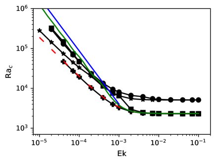
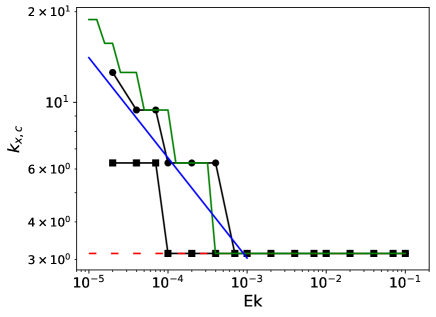
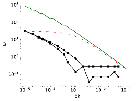
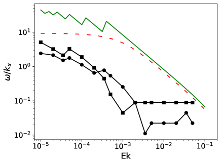
Figure 1: The critical Rayleigh number (top left), together with the wave number (top right), the frequency (bottom left), and the phase velocity (bottom right) of the critical mode at onset as a function of the Ekman number for $\frac{\Delta T}{T_{o}}=\frac{d}{H_{o}}=0.1$. The dashed red lines are the results from the linear system with constant coefficients (21,23,24) and the solid green lines are the results from the same system with $\partial_{t}\rho_{1}$ set to zero. The solid blue line indicates $\mathrm{Ra}_{c}\propto\mathrm{Ek}^{-4/3}$ in the top left and $k_{x,c}\propto\mathrm{Ek}^{-1/3}$ in the top right panels. The black symbols show the results from simulations of the full linearized equations with different boundary conditions. Pluses are free slip plates with periodic lateral boundaries, stars are also laterally periodic but have no slip plates, circles have no slip plates with free slip lateral walls, and squares have free slip boundaries in all directions and have an spect ratio of $L/d=1$.

III The linear onset

The equations (5-II) describe convection in a compressible gas rotating about an axis perpendicular to gravity. This configuration allows for vorticity generation through the compressional $\beta$-effect which is analogous the topographic $\beta$-effect familiar from rotating spherical shells or the $\beta$-plane. Previous studies of the compressional $\beta$-effect were based on the anelastic approximation Evonuk (2008); Glatzmaier, Evonuk, and Rogers (2009); Verhoeven and Stellmach (2014) in which case the equation for the vorticity component along the rotation axis is exactly the same for all the different instances of the $\beta$-effect. This leads to the expectation that, all other parameters held constant, the critical Rayleigh number should scale Busse and Simitev (2014) as $\mathrm{Ek}^{-4/3}$, and the wavenumber of the critical mode should scale as $\mathrm{Ek}^{-1/3}$.

It was also noted that there are issues with the predictions of some variants of the anelastic approximation concerning the onset of convection which appear if some velocity becomes comparable to the speed of sound, as for example the drift velocity of the critical mode Verhoeven and Glatzmaier (2018). In rotating Rayleigh-Bénard convection in which rotation and gravity are aligned with each other, the critical modes drift at onset at low Prandtl numbers. This drift can be fast enough so that the time derivative term in the continuity equation must be retained Calkins, Julien, and Marti (2015). A more comprehensive point of view was adopted by Wood and Bushby (2016) who investigated general linearized sound proof models and argued that meaningful results can only be expected if the equations conserve energy. Within this class of approximations, Wood and Bushby (2016) identified only a single set of equations whose dispersion relation is identical to that of the linearized full equations, and this approximation is different from the anelastic approximation on which most previous work is based Braginsky and Roberts (1995).

The current state of knowledge provides us with the motivation to investigate the onset of convection in some detail and by two different means. First of all, one can drop all nonlinear terms from eqs. (5-II), time step the resulting equations and compute energy as a function of time. After transients, the energy decays or increases depending on whether the Rayleigh number is below or above its critical value, and the energy stays constant if the Rayleigh number is marginal.

Since our main interest is in the weakly compressible flows realized in experiments, we will also turn in a second approach to the simplified equations (21,23,24). These equations are linear and in addition have constant coefficients. They therefore admit solutions of the form

$$\frac{\rho_{1}}{\rho_{o}}={\tilde{\rho}}e^{i\bm{k}\cdot\bm{r}}e^{\sigma t}~{}~{}~{},~{}~{}~{}T_{1}={\tilde{T}_{1}}e^{i\bm{k}\cdot\bm{r}}e^{\sigma t}~{}~{}~{},~{}~{}~{}\bm{v}=\bm{\tilde{v}}e^{i\bm{k}\cdot\bm{r}}e^{\sigma t}$$ (25)

where ${\tilde{\rho}}$, ${\tilde{T}_{1}}$ and $\bm{\tilde{v}}$ are complex amplitudes independent of space and time and $\sigma$ is a complex growth rate. The linear onset problem in 2D then reduces to the computation of the eigenvalues of a $4\times 4$ matrix. We will want to take advantage of such a dramatic simplification and determine critical Rayleigh numbers from this purely algebraic problem. Even though this is a much simpler problem than the original eigenvalue problem posed by the linearized partial differential equations, only numerical evaluations of the eigenvalues of the $4\times 4$ matrix are practical.

Solutions in the form of plane waves ignore the presence of boundaries. To emulate boundaries, we restrict the admissible wavenumbers in eq. (25) to $k_{z}=\pi$ and $k_{x}=n\pi$ with $n=1,2,3,...$. The solutions obtained from the matrix problem will be compared to different sets of boundary conditions implemented in the direct numerical simulations of the full linearized equations. Periodic boundary conditions in the directions perpendicular to gravity accommodate plane waves at least in this direction, so that we will solve the full linear onset problem both with free slip and adiabatic sidewalls, and with periodic lateral boundary conditions, but never with no slip sidewalls. Plane waves can be superposed so that the dependence on $z$ is a sine or cosine function which satisfies free slip boundary conditions, so that the full eigenvalue problem will also be solved with stress free boundary conditions for the purpose of comparison, in addition to the no slip boundary conditions which are implemented in the nonlinear simulations of the next sections and which are most relevant for the simulation of experiments.

Fig. 1 summarizes the results for $\frac{\Delta T}{T_{o}}=\frac{d}{H_{o}}=0.1$. These parameters are typical for a laboratory experiment and they are small enough so that the simplifications leading to eqs. (21,23,24) seem justified. The critical Rayleigh number $\mathrm{Ra_{c}}$ obtained from the matrix problem agrees remarkably well with the $\mathrm{Ra_{c}}$ obtained from the onset calculation for free slip boundaries with periodic lateral boundary conditions. However, the dependence of $\mathrm{Ra_{c}}$ on $\mathrm{Ek}$ in these two cases is different from the $\mathrm{Ek}^{-4/3}$ expected from the anelastic approximation, and the wavenumber $k_{x}$ of the critical mode (which is restricted to integer multiples of $\pi$) is independent of $\mathrm{Ek}$. The computed $\mathrm{Ra_{c}}$ behaves approximately as $\mathrm{Ra_{c}}\propto\mathrm{Ek}^{-1}$.

To elucidate the origin of this discrepancy, the matrix problem was also solved after omitting the term $\partial_{t}\rho_{1}$ from eq. (24). The equation of continuity then has the same form as in the anelastic approximation. The critical Rayleigh number obtained from this somewhat artificial problem is also shown in fig. 1. At small Ekman numbers, one finds $\mathrm{Ra_{c}}\propto\mathrm{Ek}^{-4/3}$ and $k_{c}\propto\mathrm{Ek}^{-1/3}$ as predicted by the anelastic approximation. When the Ekman number is large and rotational effects are negligible, the onset of convection is stationary and the computed $\mathrm{Ra_{c}}$ is of course independent of whether the term $\partial_{t}\rho_{1}$ was included or not. But at $\frac{\Delta T}{T_{o}}=\frac{d}{H_{o}}=0.1$, an $\mathrm{Ek}$ of $10^{-3}$ or less is already enough to produce a very noticeable discrepancy between the two forms of the continuity equation. The scalings $\mathrm{Ra_{c}}\propto\mathrm{Ek}^{-4/3}$ and $k_{c}\propto\mathrm{Ek}^{-1/3}$ apparently require the linearized equation of continuity as it appears in the anelastic approximation, which is

$$v_{z}\left(\frac{\Delta T}{T_{o}}-\gamma\frac{d}{H_{o}}\right)+\nabla\cdot\bm{v}=0.$$ (26)

This equation imposes a constraint on the structure of the velocity field that the critical mode of the full problem apparently does not satisfy. The imaginary part of $\sigma$ still is small compared with the inverse of the travel time of sound waves across the cell or the rotation rate of the frame of reference so that the reasons for the failure of the anelastic approximation identified by Verhoeven and Glatzmaier (2018) do not apply here. But the imaginary part of $\sigma$ is large enough so that the time derivative term needs to be retained in the equation of continuity. Rapid oscillations in the critical mode have already been found to be an obstacle for the anelastic approximation in rotating Rayleigh-Bénard convection in plane layers Calkins, Julien, and Marti (2015) and in convection in rotating spherical shells Liu et al. (2019).

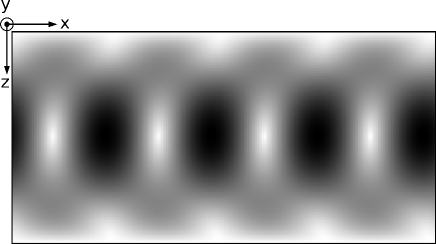
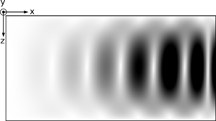
Figure 2: Snapshots of the velocity magnitude $|\bm{v}|$ obtained from the full linearised equations. The boundary conditions are no-slip in $z$, free slip in $y$ and periodic (left panel) or free slip (right panel) in $x$. Both simulations are for $\mathrm{Ek}=4\times 10^{-5}$ and $\mathrm{Ra}$ close to the critical Rayleigh number ($\mathrm{Ra}=7.4\times 10^{4}$ in the left panel and $\mathrm{Ra}=1.3\times 10^{5}$ in the right panel). These snapshots are extracted from animations contained in the supplementary material.

We now turn to the stability limits determined from the full linearized equations. As already mentioned, periodic lateral boundary conditions with free slip conditions in $z$ lead to convincing agreement with the algebraic problem. The critical Rayleigh number increases if the boundary conditions become no slip, more so with sidewalls than with periodic lateral boundary conditions. We also performed a series of computations with free slip conditions in $z$ together with sidewalls, separated by only 1 nondimensional unit as opposed to 2 for all the other computations. The marginal mode of the periodic case still fits into this box with stress free sidewalls. The critical mode drifts because of the compressional $\beta$-effect in the periodic case at small $\mathrm{Ek}$. Sidewalls obviously are an obstacle to the drift. Perhaps surprisingly, the critical mode still drifts in the presence of sidewalls. Wavecrests are continuously generated at one sidewall which grow in amplitude while they travel to the opposite sidewall where they are annihilated. Snapshots taken from animations included in the supplemental material and shown in fig. 2 exemplify this behavior. The sidewalls reduce the oscillation frequency of the mode and its phase velocity, but the time dependence remains fast enough to invalidate the prediction of the anelastic approximation for $\mathrm{Ra_{c}}$.

The drift velocity for no slip boundaries is neither systematically larger nor smaller than for free slip boundaries, and the oscillation frequencies seem to converge to each other at small $\mathrm{Ek}$ for both types of boundary conditions.

IV Comparison of 2D and 3D convection

This section will compare compressible 2D and 3D convection in nonrotating frames. We start from the assumption that there are combinations of parameters at which spanwise rotation forces convection to be 2D but has no additional effect on the flow. Assuming such a 2D flow is realized, how does it differ from 3D nonrotating convection at the same $\mathrm{Ra}$, $\mathrm{Pr}$, $\frac{d}{H_{o}}$ and $\frac{\Delta T}{T_{o}}$? To answer this question, we take advantage of the database on 3D compressible convection in ref. Tilgner, 2011 and run 2D simulations at the exact same parameters.

The most elementary quantities to be compared are of course the kinetic energy density $E_{\mathrm{kin}}$

$$E_{\mathrm{kin}}=\langle\frac{1}{V}\int\frac{1}{2}\rho\bm{v}^{2}dV\rangle$$ (27)

where the integration extends over the entire volume $V$ in 3D or area in 2D. Angular brackets denote time average. The characteristic velocity is determined by the Peclet number $\mathrm{Pe}$

$$\mathrm{Pe}=\sqrt{\langle\frac{1}{V}\int\bm{v}^{2}dV\rangle}$$ (28)

which is called Peclet number because velocity has been made nondimensional by the velocity scale $\kappa_{o}/d$. The heat injected into the fluid is the heat traversing the warm boundary and serves to define the Nusselt number $\mathrm{Nu}$ in

$$\mathrm{Nu}=-\langle\frac{1}{A}\int\partial_{z}TdA\rangle$$ (29)

where $A$ is the area (or length in the 2D case) of the warm boundary. The isentropic state in the model considered here has a uniform temperature gradient with a temperature difference $\Delta T_{\mathrm{ad}}$ between the temperature regulated boundaries of

$$\frac{\Delta T_{\mathrm{ad}}}{\Delta T}=(\gamma-1)\frac{T_{o}}{\Delta T}\frac{d}{H_{o}}=\frac{gd}{C_{p}\Delta T}.$$ (30)

The Nusselt number $\mathrm{Nu}_{*}$ based on the superadiabatic heat flux is thus defined as

$$\mathrm{Nu}_{*}=\frac{\mathrm{Nu}-\Delta T_{\mathrm{ad}}/\Delta T}{1-\Delta T_{\mathrm{ad}}/\Delta T}.$$ (31)

It is useful to similarly define a Rayleigh number $\mathrm{Ra}_{*}$ based on the superadiabatic temperature difference as

$$\mathrm{Ra}_{*}=\frac{gd^{3}(\Delta T-\Delta T_{\mathrm{ad}})}{T_{o}\kappa_{o}\nu_{o}}=\mathrm{Ra}\left(1-(\gamma-1)\frac{d}{H_{o}}\frac{T_{o}}{\Delta T}\right).$$ (32)

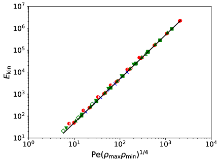
Figure 3: The kinetic energy density as a function of $\mathrm{Pe}(\rho_{\mathrm{max}}\rho_{\mathrm{min}})^{1/4}$. The symbols are the same as in ref. Tilgner, 2011 with $\Delta T_{\mathrm{ad}}/\Delta T=1/15$ (blue symbols) and $\Delta T/T_{o}=0.1$ (plus) or $1$ (x), $\Delta T_{\mathrm{ad}}/\Delta T=2/3$ (green symbols) and $\Delta T/T_{o}=0.1$ (empty squares), $0.3$ (full squares), $1$ (empty triangle up), $3$ (full triangle up), $10$ (empty triangle down), $30$ (full triangle down), and $100$ (empty diamonds), and $\Delta T_{\mathrm{ad}}/\Delta T=4/5$ (red symbols) and $\Delta T/T_{o}=0.1$ (empty circles), $1$ (full circles), and $10$ (half filled circles).

$E_{\mathrm{kin}}$ and $\mathrm{Pe}$ describe the same property in incompressible fluids. In a compressible gas, however, the relation between $E_{\mathrm{kin}}$ and $\mathrm{Pe}$ depends on an effective density. It was found for 3D convection Tilgner (2011) that $E_{\mathrm{kin}}$ and $\mathrm{Pe}$ are related by

$$E_{\mathrm{kin}}=\frac{1}{2}\sqrt{\rho_{\mathrm{max}}\rho_{\mathrm{min}}}~{}\mathrm{Pe}^{2}$$ (33)

where $\rho_{\mathrm{max}}$ and $\rho_{\mathrm{min}}$ are the maximum and minimum of the density profiles obtained after averaging $\rho(\bm{r},t)$ over time, $x$ and $y$. The exact same relation holds in 2D (see fig. 3) so that $\sqrt{\rho_{\mathrm{max}}\rho_{\mathrm{min}}}$ acts as effective density both in 3D and in 2D.

Convection in a compressible gas also differs from convection within the Boussinesq approximation in that the two thermal boundary layers near the temperature regulated boundaries are not symmetric to each other Jones, Mizerski, and Kessar (2022). One can compute velocities from quantities local to each boundary layer. There is a free fall velocity, which depends on the density and temperature profiles within the boundary layers, and there are the maximal velocities parallel to the boundaries. There are two relations connecting these velocities in 3D convection (figs. 8 and 9 in ref. Tilgner, 2011) and these relations are again valid in 2D.

Other quantities of interest are detectably different in 2D and 3D. Since 2D and 3D data are available for the same control parameters, we can directly compare the superadiabatic Nusselt number for 2D flow, $\mathrm{Nu}_{*,2D}$, with its analog in 3D convection, $\mathrm{Nu}_{*,3D}$. As seen in fig. 4, the two Nusselt numbers are equal at small $\mathrm{Nu}_{*}$ and $\mathrm{Nu}_{*,2D}$ becomes smaller than $\mathrm{Nu}_{*,3D}$ for large $\mathrm{Nu}_{*}$. However, the difference between the Nusselt numbers is always less than 20% in fig. 4.

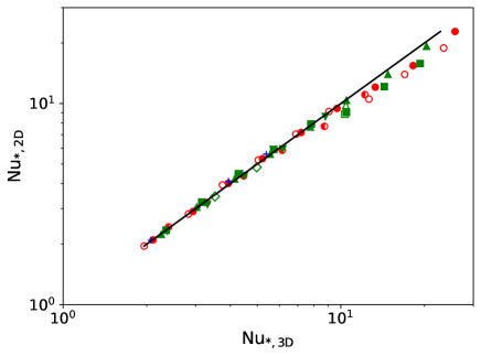
Figure 4: Comparison between $\mathrm{Nu}_{*}$ in the 3D simulations from ref. Tilgner, 2011, $\mathrm{Nu}_{*,3D}$, and the 2D simulations at the identical control parameters, $\mathrm{Nu}_{*,2D}$. The symbols are the same as in Figure 3. The black line is the diagonal $\mathrm{Nu}_{*,3D}=\mathrm{Nu}_{*,2D}$.

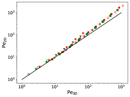
Figure 5: Comparison between $\mathrm{Pe}$ in the 3D simulations from ref. Tilgner, 2011, $\mathrm{Pe}_{3D}$, and the 2D simulations at the identical control parameters, $\mathrm{Pe}_{2D}$. The symbols are the same as in Figure 3. The black line is the diagonal $\mathrm{Pe}_{3D}=\mathrm{Pe}_{2D}$.

A considerably larger effect is visible in the Peclet number in going from its value in 2D, $\mathrm{Pe}_{2D}$, to its magnitude in 3D, $\mathrm{Pe}_{3D}$. Again, the two Peclet numbers are identical at small $\mathrm{Pe}$, but at $\mathrm{Pe}\gtrsim 30$, $\mathrm{Pe}_{2D}$ exceeds $\mathrm{Pe}_{3D}$. The marginally stable mode of the linear stability problem is two dimensional. It therefore is not surprising that the two Peclet numbers are equal near onset when $\mathrm{Pe}$ is small. If on the contrary the Peclet number is large, the flow is likely prone to 3D instabilities and the nonlinear advection term becomes important. Nonlinearity ultimately leads to turbulence, which notoriously behaves differently in 2D and 3D. Nonlinearity in 3D also adds a toroidal component to the purely poloidal velocity field of the marginally stable mode, whereas 2D flows always are purely poloidal. The increasing fraction of toroidal velocity in 3D convection was already shown in Boussinesq convection to lead to different global properties in 2D and 3D convection Schmalzl, Breuer, and Hansen (2004). One therefore expects to see that the Peclet numbers become different at large $\mathrm{Pe}$, but it is not obvious why $\mathrm{Pe}_{2D}$ should become larger than $\mathrm{Pe}_{3D}$, and even less so why simultaneously $\mathrm{Nu}_{*,2D}$ becomes smaller than $\mathrm{Nu}_{*,3D}$.

The difference in $\mathrm{Nu}$ and $\mathrm{Pe}$ revealed by direct comparison between 2D and 3D implies that the scaling laws relating the observables to control parameters are different in 2D and 3D. For instance, we find

$$\mathrm{Nu}_{*,3D}-1=\frac{2}{7}(E_{\mathrm{kin}}\sqrt{\rho_{\mathrm{max}}\rho_{\mathrm{min}}})^{1/3}$$ (34)

$$\mathrm{Nu}_{*,2D}-1=0.355(E_{\mathrm{kin}}\sqrt{\rho_{\mathrm{max}}\rho_{\mathrm{min}}})^{0.283}$$ (35)

and

$$\mathrm{Nu}_{*,3D}=0.22\left(\mathrm{Ra}_{*}(\rho_{\mathrm{max}}\rho_{\mathrm{min}})^{1/4}\right)^{0.265}$$ (36)

$$\mathrm{Nu}_{*,2D}=0.275\left(\mathrm{Ra}_{*}(\rho_{\mathrm{max}}\rho_{\mathrm{min}})^{1/4}\right)^{0.25}$$ (37)

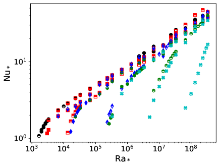
Figure 6: $\mathrm{Nu}_{*}$ as a function of $\mathrm{Ra}_{*}$ for $\Delta T/T_{o}=d/H_{o}=0.1$ (filled symbols), $\Delta T/T_{o}=d/H_{o}=0.01$ (filled in bottom half), and $\Delta T/T_{o}=d/H_{o}=1$ (filled in top half). Symbols indicate nonrotating flows (black circles) and the Ekman numbers $\mathrm{Ek}=10^{-3}$ (red squares), $\mathrm{Ek}=10^{-4}$ (blue diamonds), $\mathrm{Ek}=10^{-5}$ (green hexagons), and $\mathrm{Ek}=10^{-6}$ (cyan plus).

V Transitions

The previous section omitted the Coriolis force. We will now reinstate the Coriolis force and solve the equations (5-II) in 2D to determine the region in the $(\mathrm{Ra},\mathrm{Ek})-$plane in which rotational effects are important. The resulting Nusselt number is shown in fig. 6. This figure is for $\frac{\Delta T}{T_{o}}=\frac{d}{H_{o}}=0.1$ representative of experimental parameters as well as for $\frac{\Delta T}{T_{o}}=\frac{d}{H_{o}}=1$, and $\frac{\Delta T}{T_{o}}=\frac{d}{H_{o}}=0.01$. One recognizes that the onset is delayed by rotation. As the Rayleigh number is increased beyond its critical value, one first observes a steep increase of $\mathrm{Nu}$ as a function of $\mathrm{Ra}$ until the $\mathrm{Nu}(\mathrm{Ra})$ dependence asymptotically approaches the same dependence as in the nonrotating case.

This figure qualitatively explains fig. 9 of Menaut et al. (2019) in which one sees a scaling in $\mathrm{Nu}\propto\mathrm{Ra}^{0.3}$ typical of nonrotating convection at large $\mathrm{Ra}$, together with a steeper and Ekman number dependent $\mathrm{Nu}(\mathrm{Ra})$ at low $\mathrm{Ra}$. Menaut et al. (2019) also report a hysteresis in which $\mathrm{Nu}(\mathrm{Ra})$ continues to follow the scaling of nonrotating convection if $\mathrm{Ra}$ is lowered from large values down to the range in which the Ekman number dependent scaling is observed if $\mathrm{Ra}$ is increased starting from small values. A hysteresis of this type could not be reproduced in the simulations, possibly because the Ekman number in the simulations is orders of magnitudes larger than in the experiments.

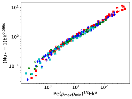
Figure 7: The same data as in Figure 6 with the same symbols represented as $(\mathrm{Nu}_{*}-1)\mathrm{Ek}^{0.566\alpha}$ as a function of $\mathrm{Pe}\sqrt{\rho_{\mathrm{max}}\rho_{\mathrm{min}}}\mathrm{Ek}^{\alpha}$ with $\alpha=0.36$.

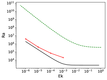
Figure 8: Shown are three transition lines in the $(\mathrm{Ek},\mathrm{Ra})-$plane with the onset of convection as the solid black line, the transition from 2D to 3D convection as the dashed green line, and the transition from rotation dependent to rotation independent scaling of the Nusselt number as the red pluses.

Similar transitions from flows dominated by rotation to flows nearly independent of rotation are known from other systems. Probably the best studied example is Rayleigh-Bénard convection with collinear rotation and gravity axes Ecke and Shishkina (2023). Schmitz and Tilgner (2009) presented a data reduction leading to a criterion for the transition between both types of flows based on the Ekman and Peclet numbers. The success of this data reduction relies on simple scaling laws valid either near the onset of convection or in the strongly driven regime. An equally satisfactory data collapse cannot be expected in the compressible case because of the large number of control parameters, and because it is not trivial to determine a scaling for the Nusselt number close to onset. Inspired by the example of rotating Rayleigh-Bénard convection, we represent $(\mathrm{Nu}_{*}-1)\mathrm{Ek}^{0.566\alpha}$ as a function of $\mathrm{Pe}\sqrt{\rho_{\mathrm{max}}\rho_{\mathrm{min}}}\mathrm{Ek}^{\alpha}$. The factor $0.566$ in the exponent guarantees for arbitrary $\alpha$ that the Peclet number dependence of $\mathrm{Nu}_{*}$ in nonrotating convection in eq. (37) will appear as a straight line in a double logarithmic plot. The exponent $\alpha$ is optimized to collapse the data on a single curve as well as possible. An optimum exists near $\alpha=0.36$ which leads to fig. 7. The nonrotating asymptote is reached for $\mathrm{Pe}\sqrt{\rho_{\mathrm{max}}\rho_{\mathrm{min}}}\mathrm{Ek}^{0.36}\gtrsim 1$, whereas the data points fan out below this transition point and the Nusselt number differs from nonrotating convection. There is of course some uncertainty where exactly to localize the transition so that we give the most weight to the computations with $\frac{\Delta T}{T_{o}}=\frac{d}{H_{o}}=0.1$ which are close to experimental conditions. Once one has defined the Peclet number at which the transition occurs, one can use the $\mathrm{Pe}(\mathrm{Ra})$ dependence to find the transitional Rayleigh number for every Ekman number. This procedure results in a line in the $(\mathrm{Ek},\mathrm{Ra})-$plane which separates flows subject to a sufficiently strong $\beta-$effect to modify the Nusselt number from flows whose Nusselt number is indistinguishable from that of nonrotating 2D convection.

This line is shown in fig. 8 together with the approximate stability limit of 2D flows. The transition from 2D to 3D flow was not tracked by direct simulation but was instead deduced from the stability criterion for elliptic instability. It was shown in ref. Lüdemann and Tilgner, 2022 that 2D flows in convection cells with spanwise rotation are unstable to 3D perturbations because of the finite ellipticity of the streamlines of the convection rolls. The elliptical instability is inoperative if the streamlines are either parallel or circular. There is therefore some ellipticity at which the convection rolls are least stable. The stability limit for this ellipticity was computed according to the method detailed in ref. Lüdemann and Tilgner, 2022 which first yields a stability curve in the $(\mathrm{Ek},\mathrm{Pe})-$plane which must be converted to a stability curve in the $(\mathrm{Ek},\mathrm{Ra})-$plane with the help of the $\mathrm{Pe}(\mathrm{Ra})$ dependence. Combinations of $\mathrm{Ek}$ and $\mathrm{Ra}$ below this stability line in fig. 8 are certainly 2D.

Fig. 8 contains one last stability criterion which simply is the linear onset of convection. In summary, one finds that at small Ekman numbers and the compressibility typical of laboratory experiments, there are roughly four orders of magnitude in $\mathrm{Ra}$ beyond the critical Rayleigh number for which the flow stays two dimensional, and out of these four orders of magnitude, there is a factor of $3$ to $10$ in $\mathrm{Ra}$ for which the heat transport is reduced from its value in nonrotating convection. There are thus at least 3 decades in $\mathrm{Ra}$ in which the experiments can approximate 2D nonrotating compressible convection.

VI Mean flow

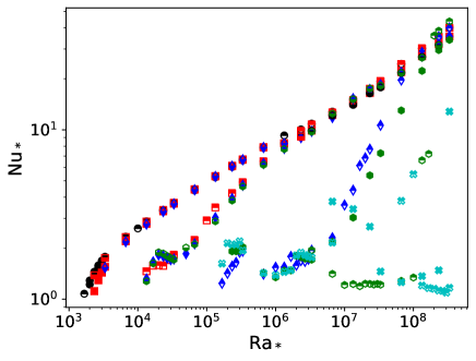
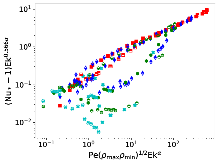
Figure 9: $\mathrm{Nu}_{*}$ as as function of $\mathrm{Ra}*$ (left panel) and $(\mathrm{Nu}_{*}-1)\mathrm{Ek}^{0.566\alpha}$ as a function of $\mathrm{Pe}\sqrt{\rho_{\mathrm{max}}\rho_{\mathrm{min}}}\mathrm{Ek}^{\alpha}$ for $\alpha=0.36$ (right panel) for the same parameters and with the same symbols as in Figure 6 but for periodic conditions in the $x-$direction.

We have seen in section III that sidewalls slow down the drifting motion of the critical mode at onset, but not enough so to make a qualitative difference. Another possible effect of sidewalls is the suppression of mean flows. Experimentally, one can either use cylindrical cells Jiang et al. (2020) which allow mean flows or rectangular cells Menaut et al. (2019) which inhibit mean flows. An accurate numerical representation of a cylindrical annulus would require a cylindrical computational volume, or at least a Cartesian geometry with periodic lateral boundary conditions with a large aspect ratio. However, we chose to run simulations in the Cartesian geometry with no slip boundaries in $z$ and periodic sidewalls with an aspect ratio of only 2 to allow for direct comparison with the results of the previous sections.

Fig. 9 shows the Nusselt number obtained with these boundary conditions for 2D convection. At large $\mathrm{Ra}$, all curves approach a common asymptote which corresponds to nonrotating convection. At $\mathrm{Ra}$ slightly above onset, the Nusselt number behaves very differently from the case with sidewalls in fig. 6. The heat transport is suppressed by the presence of a mean flow. This mean flow has both a shearing component and a general drift in prograde direction. It is known that the amplitude of mean flows depends on the aspect ratio of the computational volume if that aspect ratio is modest van der Poel et al. (2014). A detailed study of the mean flow was not undertaken for this reason. But it now is obvious that the subdivison of the parameter space in fig. 8 looks qualitatively the same if we change the lateral boundary condition, except that the boundary between rotation dominated and 2D nonrotating behavior is displaced. Furthermore, the dependences of $\mathrm{Nu}$ or $\mathrm{Pe}$ on the control parameters are affected by the lateral boundary conditions.

VII Conclusion

The simulations presented in this paper investigate the different types of flows that may be expected in a rectangular convection cell filled with compressible gas placed in a centrifuge. The compressibility leads to a compressional $\beta$-effect which causes the critical mode at onset to drift. This drift is slowed but not removed by sidewalls and leads to a time dependence fast enough so that the time derivative term in the continuity equation is not negligible as would be necessary for the anelastic approximation to be applicable. This effect must be expected to persist in different geometries of astrophysical relevance, such as a spherical shell.

Three distinct types of flow are accessible to convection experiments in a centrifuge according to theory and numerical simulations: convection in which global rotation is fast enough to force the flow to be 2D and in which the compressional $\beta$-effect causes a drift and limits the heat flow, 2D convection which behaves like nonrotating 2D convection in as far as the heat flow is concerned, and 3D convection. It is not excluded that the anelastic approximation becomes useful again once the Rayleigh number is large enough so that the influence of the compressional $\beta$-effect on the heat flow becomes small.

The 2D convection can only serve as an approximate model for 3D convection since the scaling laws for heat flux and kinetic energies are not exactly the same, even though other properties are identical. For instance, the boundary layers near the temperature regulated boundaries are not symmetric to each other because the density in the one is different form the density in the other. However, velocity scales pertaining to the boundary layers are connected by the same relationships in both dimensions.

Numerical simulations of course cannot reproduce the extreme control parameters accessible to experiments which may lead to new surprising results in the experiments. The existing experimental data show that there is a hysteresis in the heat flux when the rotation rate is varied. This behavior was not seen in the numerical simulations and the physical mechanism underlying such a hysteresis remains to be understood.