Interest rate convexity in a Gaussian framework

Abstract.

The contributions of this paper are twofold: we define and investigate the properties of a short rate model driven by a general Gaussian Volterra process and, after defining precisely a notion of convexity adjustment, derive explicit formulae for it.

1. Introduction and notations

1.1. Introduction

In fixed income markets, the different schedules of payments and the diverse currencies, margins require specific adjustments in order to price all interest rate products consistently. This is usually referred to as convexity adjustment and has a deep impact on interest rate derivatives. Starting from [6, 8, 17], academics and practitioners alike have developed a series of formulae for this convexity adjustment in a variety of models, from simple stochastic rate models [14] to some incorporating stochastic volatility features [2]. Recently, Garcia-Lorite and Merino [10] used Malliavin calculus techniques to compute approximations of this convexity adjustment for various interest rate products.

Motivated by the new paradigm of rough volatility in Equity markets [4, 5, 7, 9, 11, 12, 13], we consider here stochastic dynamics for the short rate, driven by a general Gaussian Volterra process, providing more flexibility than standard Brownian motion. In the framework of the change of measure approach in [16], we introduce a clear definition of convexity adjustment, for which we are able to derive closed-form expressions.

We introduce the model, derive its properties in Section 2. In Section 2.2, we define convexity adjustment and provide formulae for it, the main result of the paper, which we illustrate in some specific examples. Section 3 provides some further expressions for liquid interest rate products, and we highlight some numerical aspects of the results in Section 4.

1.2. Model and notations

On a given filtered probability space $(\Omega,\mathcal{F},(\mathcal{F}_{t})_{t\geq 0},\mathbb{P})$, we are interested in short rate dynamics of the form

(1.1) $$r_{t}=\theta(t)+\int_{0}^{t}\varphi(t,u)\mathrm{d}\mathfrak{W}_{u}=\theta(t)+\left(\varphi(t,\cdot)\circ\mathfrak{W}\right)_{t},$$

where $\theta$ is a deterministic function and $\mathfrak{W}$ a continuous Gaussian process adapted to the filtration $(\mathcal{F}_{t})_{t\geq 0}$. Here and below, given a function $\varphi$ and a stochastic process $X$, we write $(\varphi\circ X)_{a,b}:=\int_{a}^{b}\varphi(s)\mathrm{d}X_{s}$, and omit $a$ whenever $a=0$. Define further, for $u\leq t\leq T$,

(1.2) $$\Xi_{T}(t,u):=-\int_{t}^{T}\varphi(s,u)\mathrm{d}s\qquad\text{and}\qquad\Xi_{T}(u):=\Xi_{T}(u,u)$$

as well as $\Theta_{t,T}:=\displaystyle\int_{t}^{T}\theta(s)\mathrm{d}s$. We consider a given risk-neutral probability measure $\mathbb{Q}$, equivalent to $\mathbb{P}$, so that the price of the zero-coupon bond at time $t$ is given by

(1.3) $$P_{t,T}:=\mathbb{E}^{\mathbb{Q}}_{t}\left[B_{t,T}\right],\qquad\text{where}\qquad B_{t,T}:=\exp\left\{-\int_{t}^{T}r_{s}\mathrm{d}s\right\},$$

and we define the instantaneous forward rate process as

(1.4) $$f_{t,T}:=-\partial_{T}\log P_{t,T}.$$

Remark 1.1.

For modelling purposes, we shall consider kernels of convolution type, namely

(1.5) $$\varphi(t,u)=\varphi(t-u).$$

2. Gaussian martingale driver

2.1. Dynamics of the zero-coupon bond price

We assume first that $\mathfrak{W}$ is a Gaussian martingale with $\gamma_{\mathfrak{W}}(t):=\mathbb{E}[\mathfrak{W}_{t}^{2}]$ finite for all $t\geq 0$. In order to ensure existence of the rate process in (1.1), we assume the following:

Assumption 2.1.

For each $t\in[0,T]$, $\varphi(t,\cdot)\in L^{1}(\mathrm{d}\lambda)\cap L^{2}(\gamma_{\mathfrak{W}})$, and $\varphi$ is of convolution type (1.5).

Lemma 2.2.

Under Assumption 2.1, for any $T\geq 0$, $\left(\Xi_{T}(t,\cdot)\circ\mathfrak{W}\right)_{t}$ is an $(\mathcal{F}_{t})_{t\in[0,T]}$ Gaussian semimartingale.

Proof.

Note that from (1.2), $\Xi_{T}$ is in general not in convolution form (1.5). However, since  $\varphi$ is, we can write

$$\Xi_{T}(t,u):=-\int_{t}^{T}\varphi(s,u)\mathrm{d}s=-\int_{t}^{T}\varphi(s-u)\mathrm{d}s=\Phi(T-u)-\Phi(t-u),$$

where the function $\Phi$ is defined as $\Phi(z):=-\int_{\cdot}^{z}\varphi(u)\mathrm{d}u$. The stochastic integral then reads

$$\left(\Xi_{T}(t,\cdot)\circ\mathfrak{W}\right)_{t}=\int_{0}^{t}\Xi_{T}(t,u)\mathrm{d}\mathfrak{W}_{u}=-\int_{0}^{t}\left[\Phi(t-u)-\Phi(T-u)\right]\mathrm{d}\mathfrak{W}_{u},$$

which corresponds to a two-sided moving average process in the sense of [3, Section 5.2]. Assumption 2.1 then implies that for each $t\in[0,T]$, the function $\Xi_{T}(t,\cdot)$ is absolutely continuous on $[0,t]$ and $\partial_{t}\Xi_{T}(t,\cdot)\in L^{2}(\gamma_{\mathfrak{W}})$ and the statement follows from [3, Theorem 5.5]. ∎

Remark 2.3.

• The $L^{2}$ property ensures that the stochastic integral $(\varphi(t-\cdot)\circ\mathfrak{W})_{t}$ is well defined.

• The assumption does not imply that the short rate process itself, while Gaussian, is a semimartingale.

Proposition 2.4.

The price of the zero-coupon bond at time $t$ reads

$$P_{t,T}=\exp\left\{-\Theta_{t,T}+\frac{1}{2}\int_{t}^{T}\Xi_{T}(u,u)^{2}\mathrm{d}u+\left(\Xi_{T}(t,\cdot)\circ\mathfrak{W}\right)_{t}\right\},$$

and the discounted bond price $\widetilde{P}_{t,T}:=P_{t,T}\exp\left\{-\int_{0}^{t}r_{s}\mathrm{d}s\right\}$ is a $\mathbb{Q}$-martingale satisfying

$$\frac{\mathrm{d}\widetilde{P}_{t,T}}{\widetilde{P}_{t,T}}=\Xi_{T}(t,t)\ \mathrm{d}\mathfrak{W}_{t}.$$

Corollary 2.5.

The instantaneous forward rate satisfies $f_{TT}=r_{T}$ and, for all $t\in[0,T)$,

$$f_{t,T}=\theta(T)+\int_{0}^{t}\varphi(T,u)\mathrm{d}\mathfrak{W}_{u}+\int_{t}^{T}\varphi(T,u)\Xi_{T}(u,u)\mathrm{d}u.$$

In differential form, for any fixed $T>0$, for $t\in[0,T]$, this is equivalent to

$$\mathrm{d}f_{t,T}=\varphi(T-t)\mathrm{d}\mathfrak{W}_{t}-\varphi(T-t)\Xi_{T}(t,t)\mathrm{d}t.$$

Algorithm 2.6.

For simulation purposes, we assume a time grid of the form $\mathcal{T}:=\{0=t_{0}<t_{1}<\cdots<t_{N}=T\}$, and we discretise the stochastic integral along this grid with left-point approximations as

$$\left(\Xi_{T}(t_{i},\cdot)\circ\mathfrak{W}\right)_{t_{i}}=\int_{0}^{t_{i}}\Xi_{T}(t_{i},u)\mathrm{d}\mathfrak{W}_{u}\approx\sum_{k=0}^{i-1}\Xi_{T}(t_{i},t_{k})\left(\mathfrak{W}_{t_{k+1}}-\mathfrak{W}_{t_{k}}\right),\qquad\text{for each }i=1,\ldots,N.$$

The vector $\left(\Xi_{T}(t_{i},\cdot)\circ\mathfrak{W}\right)_{t_{i}\in\mathcal{T}}$ of stochastic integrals can then be simulated along the time mesh directly as

$$\begin{pmatrix}\left(\Xi_{T}(t_{1},\cdot)\circ\mathfrak{W}\right)_{t_{1}}\\ \vdots\\ \left(\Xi_{T}(t_{N},\cdot)\circ\mathfrak{W}\right)_{t_{N}}\\ \end{pmatrix}\approx\begin{pmatrix}\Xi_{T}(t_{1},t_{0})&&&&\\ \Xi_{T}(t_{2},t_{0})&\Xi_{T}(t_{2},t_{1})&&&\\ \vdots&\ddots&\ddots&&\\ \Xi_{T}(t_{N-1},t_{0})&\Xi_{T}(t_{N-1},t_{1})&\ldots&\Xi_{T}(t_{N-1},t_{N-2})&\\ \Xi_{T}(t_{N},t_{0})&\Xi_{T}(t_{N},t_{1})&\ldots&\Xi_{T}(t_{N},t_{N-1})\end{pmatrix}\begin{pmatrix}\mathfrak{W}_{t_{1}}-\mathfrak{W}_{t_{0}}\\ \vdots\\ \mathfrak{W}_{t_{N}}-\mathfrak{W}_{t_{N-1}}\end{pmatrix},$$

where the middle matrix is lower triangular (we omit the null terms everywhere for clarity).

Corollary 2.7.

With $\varphi(t)=\sigma\mathrm{e}^{-\kappa t}$, for some $\sigma>0$ $\mathfrak{W}=W$ a Brownian motion, $\theta(t):=r_{0}\mathrm{e}^{-\kappa t}+\mu\left(1-\mathrm{e}^{-\kappa t}\right)$, we recover exactly the Vasicek model [19], with dynamics

$$\mathrm{d}r_{t}=\kappa(\mu-r_{t})\mathrm{d}t+\sigma\mathrm{d}W_{t},\qquad\text{starting from }r_{0}.$$

Proof of Proposition 2.4.

The price of the zero-coupon bond at time $t$ then reads

$$P_{t,T}:=\mathbb{E}^{\mathbb{Q}}_{t}\left[\exp\left\{-\int_{t}^{T}r_{s}\mathrm{d}s\right\}\right] =\mathbb{E}^{\mathbb{Q}}_{t}\left[\exp\left\{-\int_{t}^{T}\left(\theta(s)+\int_{0}^{s}\varphi(s,u)\mathrm{d}\mathfrak{W}_{u}\right)\mathrm{d}s\right\}\right]$$

(2.1) $$=\mathrm{e}^{-\Theta_{t,T}}\mathbb{E}^{\mathbb{Q}}_{t}\left[\exp\left\{-\int_{t}^{T}\left(\int_{0}^{s}\varphi(s,u)\mathrm{d}\mathfrak{W}_{u}\right)\mathrm{d}s\right\}\right].$$

Using Fubini, we can write

(2.2) $$-\int_{t}^{T}\left(\int_{0}^{s}\varphi(s,u)\mathrm{d}\mathfrak{W}_{u}\right)\mathrm{d}s =-\int_{0}^{t}\left(\int_{t}^{T}\varphi(s,u)\mathrm{d}s\right)\mathrm{d}\mathfrak{W}_{u}-\int_{t}^{T}\left(\int_{u}^{T}\varphi(s,u)\mathrm{d}s\right)\mathrm{d}\mathfrak{W}_{u}$$

$$=\int_{0}^{t}\Xi_{T}(t,u)\mathrm{d}\mathfrak{W}_{u}+\int_{t}^{T}\Xi_{T}(u,u)\mathrm{d}\mathfrak{W}_{u},$$

using (1.2). Plugging this into (2.1), the zero-coupon bond then reads

$$P_{t,T} =\mathrm{e}^{-\Theta_{t,T}}\exp\left\{\int_{0}^{t}\Xi_{T}(t,u)\mathrm{d}\mathfrak{W}_{u}\right\}\mathbb{E}^{\mathbb{Q}}_{t}\left[\exp\left\{\int_{t}^{T}\Xi_{T}(u)\mathrm{d}\mathfrak{W}_{u}\right\}\right]$$

$$=\mathrm{e}^{-\Theta_{t,T}}\exp\Big{\{}\left(\Xi_{T}(t,\cdot)\circ\mathfrak{W}\right)_{t}\Big{\}}\mathbb{E}^{\mathbb{Q}}_{t}\left[\mathrm{e}^{\left(\Xi_{T}\circ\mathfrak{W}\right)_{t,T}}\right].$$

Conditional on $\mathcal{F}_{t}$, the random variable $\left(\Xi_{T}\circ\mathfrak{W}\right)_{t,T}$ is centered Gaussian with variance

$$\mathbb{V}_{t}\left[\left(\Xi_{T}\circ\mathfrak{W}\right)_{t,T}\right]=\int_{t}^{T}\Xi_{T}(u,u)^{2}\mathrm{d}u,$$

so that

$$P_{t,T}=\mathrm{e}^{-\Theta_{t,T}}\exp\left\{\left(\Xi_{T}(t,\cdot)\circ W\right)_{t}+\frac{1}{2}\int_{t}^{T}\Xi_{T}(u)^{2}\mathrm{d}u\right\}.$$

Note that, using Fubini and Assumption 2.1,

$$\left(\Xi_{T}(t,\cdot)\circ\mathfrak{W}\right)_{t}=\int_{0}^{t}\Xi_{T}(t,u)\mathrm{d}\mathfrak{W}_{u} =\int_{0}^{t}\left(\Xi_{T}(u,u)+\int_{u}^{t}\partial_{s}\Xi_{T}(s,u)\mathrm{d}s\right)\mathrm{d}\mathfrak{W}_{u}$$

$$=\int_{0}^{t}\Xi_{T}(u,u)\mathrm{d}\mathfrak{W}_{u}+\int_{0}^{t}\int_{u}^{t}\partial_{s}\Xi_{T}(s,u)\mathrm{d}s\mathrm{d}\mathfrak{W}_{u}$$

$$=\int_{0}^{t}\Xi_{T}(u,u)\mathrm{d}\mathfrak{W}_{u}+\int_{0}^{t}\int_{0}^{s}\partial_{s}\Xi_{T}(s,u)\mathrm{d}\mathfrak{W}_{u}\mathrm{d}s$$

$$=\int_{0}^{t}\Xi_{T}(u,u)\mathrm{d}\mathfrak{W}_{u}+\int_{0}^{t}\int_{0}^{s}\varphi(s,u)\mathrm{d}\mathfrak{W}_{u}\mathrm{d}s.$$

This is an $L^{1}$-Dirichlet process [18, Definition 2], written as a decomposition of a local martingale and a term with zero quadratic variation. Therefore $\langle\log(P_{\cdot,T}),\log(P_{\cdot,T})\rangle_{t}=\int_{0}^{t}\Xi_{T}(u,u)^{2}\mathrm{d}u$ and

(2.3) $$\mathrm{d}\log(P_{\cdot,T})=\left(\theta(t)+\left(\partial_{t}\Xi_{T}(t,\cdot)\circ\mathfrak{W}\right)_{t}-\frac{1}{2}\Xi_{T}(t)^{2}\right)\mathrm{d}t+\Xi_{T}(t,t)\mathrm{d}\mathfrak{W}_{t}.$$

Now, Itô’s formula using (2.3) yields $P_{T,T}=P_{t,T}+\int_{t}^{T}P_{s,T}\mathrm{d}X_{s}+\frac{1}{2}\int_{t}^{T}P_{s,T}\mathrm{d}\langle X,X\rangle_{s}$, hence, for each $T>0$, $\mathrm{d}P_{T,T}=\mathrm{d}P_{t,T}-P_{t,T}\mathrm{d}X_{t}-\frac{1}{2}P_{t,T}\mathrm{d}\langle X,X\rangle_{t}$, and therefore, since $P_{T,T}=1$,

$$\frac{\mathrm{d}P_{t,T}}{P_{t,T}} =\mathrm{d}X_{t}+\frac{1}{2}\mathrm{d}\langle X,X\rangle_{t}$$

$$=\left(\underbrace{\theta(t)+\left(\partial_{t}\Xi_{T}(t,\cdot)\circ\mathfrak{W}\right)_{t}}_{r_{t}}-\frac{1}{2}\Xi_{T}(t)^{2}\right)\mathrm{d}t+\Xi_{T}(t,t)\mathrm{d}\mathfrak{W}_{t}+\frac{1}{2}\mathrm{d}\left(\int_{0}^{t}\Xi_{T}(u,u)^{2}\mathrm{d}u\right)$$

$$=r_{t}\mathrm{d}t+\Xi_{T}(t,t)\mathrm{d}\mathfrak{W}_{t}-\frac{1}{2}\Xi_{T}(t)^{2}\mathrm{d}t+\frac{1}{2}\Xi_{T}(t,t)^{2}\mathrm{d}t$$

$$=r_{t}\mathrm{d}t+\Xi_{T}(t,t)\mathrm{d}\mathfrak{W}_{t}.$$

The dynamics of the discounted zero-coupon bond price in the lemma follows immediately. ∎

Proof of Corollary 2.5.

The instantaneous forward rate process (1.4) reads

$$f_{t,T} =\partial_{T}\Theta_{t,T}-\partial_{T}\int_{0}^{t}\Xi_{T}(t,u)\mathrm{d}\mathfrak{W}_{u}-\frac{1}{2}\partial_{T}\int_{t}^{T}\Xi_{T}(u)^{2}\mathrm{d}u$$

$$=\partial_{T}\Theta_{t,T}-\partial_{T}\int_{0}^{t}\left(-\int_{t}^{T}\varphi(s,u)\mathrm{d}s\right)\mathrm{d}\mathfrak{W}_{u}-\frac{1}{2}\partial_{T}\int_{t}^{T}\left(-\int_{u}^{T}\varphi(s,u)\mathrm{d}s\right)^{2}\mathrm{d}u$$

$$=\theta(T)+\int_{0}^{t}\partial_{T}\left(\int_{t}^{T}\varphi(s,u)\mathrm{d}s\right)\mathrm{d}\mathfrak{W}_{u}-\frac{1}{2}\partial_{T}\int_{t}^{T}\left(\int_{u}^{T}\varphi(s,u)\mathrm{d}s\right)^{2}\mathrm{d}u$$

$$=\theta(T)+\int_{0}^{t}\varphi(T,u)\mathrm{d}\mathfrak{W}_{u}-\frac{1}{2}\left(\int_{T}^{T}\varphi(s,T)^{2}\mathrm{d}s+\int_{t}^{T}\partial_{T}\left[\left(\int_{u}^{T}\varphi(s,u)\mathrm{d}s\right)^{2}\right]\mathrm{d}u\right)$$

$$=\theta(T)+\int_{0}^{t}\varphi(T,u)\mathrm{d}\mathfrak{W}_{u}-\int_{t}^{T}\varphi(T,u)\left(\int_{u}^{T}\varphi(s,u)\mathrm{d}s\right)\mathrm{d}u$$

$$=\theta(T)+\int_{0}^{t}\varphi(T,u)\mathrm{d}\mathfrak{W}_{u}+\int_{t}^{T}\varphi(T,u)\Xi_{T}(u,u)\mathrm{d}u,$$

as claimed. ∎

Remark 2.8.

The two lemmas above correspond to the two sides of the Heath-Jarrow-Morton framework. From the expression of the instantaneous forward rate, let $\alpha_{t,T}:=\varphi(T-t)\Xi_{T}(t,t)$ and $\beta_{t,T}:=\varphi(T-t)$, so that $\mathrm{d}f_{t,T}=\beta_{t,T}\mathrm{d}\mathfrak{W}_{t}-\alpha_{t,T}\mathrm{d}t$, and consider the discounted bond price

$$\widetilde{P}_{t,T}:=P_{t,T}\exp\left\{-\int_{0}^{t}r_{s}\mathrm{d}s\right\}=\exp\left\{-\int_{0}^{t}r_{s}\mathrm{d}s-\int_{t}^{T}f_{t,s}\mathrm{d}s\right\}=:\mathrm{e}^{Z_{t}}.$$

Itôs’ formula then yields

(2.4) $$\frac{\mathrm{d}\widetilde{P}_{t,T}}{\widetilde{P}_{t,T}}=\mathrm{d}Z_{t}+\frac{1}{2}\mathrm{d}\langle Z,Z\rangle_{t}.$$

From the differential form of $f_{t,T}$, we can write, for any $t\in[0,T)$,

$$f_{t,T}=f_{0,T}+\int_{0}^{t}\mathrm{d}f_{s,T}=f_{0,T}+\int_{0}^{t}\Big{(}\varphi(T,u)\mathrm{d}\mathfrak{W}_{u}-\varphi(T,u)\Xi_{T}(u,u)\mathrm{d}u\Big{)}=f_{0,T}+\int_{0}^{t}\beta_{u,T}\mathrm{d}\mathfrak{W}_{u}+\int_{0}^{t}\alpha_{u,T}\mathrm{d}u,$$

so that, using stochastic Fubini, we obtain

$$F_{t,T} :=\int_{t}^{T}f_{t,s}\mathrm{d}s=\int_{t}^{T}\left(f_{0,s}+\int_{0}^{t}\beta_{u,s}\mathrm{d}\mathfrak{W}_{u}+\int_{0}^{t}\alpha_{u,s}\mathrm{d}u\right)\mathrm{d}s$$

$$=\int_{t}^{T}f_{0,s}\mathrm{d}s+\int_{0}^{t}\int_{t}^{T}\beta_{u,s}\mathrm{d}s\mathrm{d}\mathfrak{W}_{u}+\int_{0}^{t}\int_{t}^{T}\alpha_{u,s}\mathrm{d}s\mathrm{d}u.$$

Now,

$$\int_{t}^{T}f_{0,s}\mathrm{d}s =\int_{t}^{T}\left(f_{s,s}-\int_{0}^{s}\partial_{u}f_{u,s}\mathrm{d}u\right)\mathrm{d}s$$

$$=\int_{t}^{T}r_{s}\mathrm{d}s-\int_{0}^{t}\int_{t}^{T}\partial_{u}f_{u,s}\mathrm{d}s\mathrm{d}u-\int_{t}^{T}\int_{u}^{T}\partial_{u}f_{u,s}\mathrm{d}s\mathrm{d}u$$

$$=\int_{t}^{T}r_{s}\mathrm{d}s-\int_{0}^{t}\left(\int_{t}^{T}\partial_{u}f_{u,s}\mathrm{d}s-\int_{u}^{T}\partial_{u}f_{u,s}\mathrm{d}s\right)\mathrm{d}u-\int_{0}^{T}\int_{u}^{T}\partial_{u}f_{u,s}\mathrm{d}s\mathrm{d}u$$

$$=\int_{t}^{T}r_{s}\mathrm{d}s+\int_{0}^{t}\int_{u}^{t}\partial_{u}f_{u,s}\mathrm{d}s\mathrm{d}u-\int_{0}^{T}\int_{u}^{T}\partial_{u}f_{u,s}\mathrm{d}s\mathrm{d}u,$$

using Fubini, so that

$$F_{t,T}=\underbrace{\int_{t}^{T}r_{s}\mathrm{d}s+\int_{0}^{t}\int_{u}^{t}\partial_{u}f_{u,s}\mathrm{d}s\mathrm{d}u-\int_{0}^{T}\int_{u}^{T}\partial_{u}f_{u,s}\mathrm{d}s\mathrm{d}u}_{\int_{t}^{T}f_{0,s}\mathrm{d}s}+\int_{0}^{t}\int_{t}^{T}\beta_{u,s}\mathrm{d}s\mathrm{d}\mathfrak{W}_{u}+\int_{0}^{t}\int_{t}^{T}\alpha_{u,s}\mathrm{d}s\mathrm{d}u,$$

and

$$\mathrm{d}F_{t,T}=\left(\int_{t}^{T}\alpha_{t,s}\mathrm{d}s-r_{t}\right)\mathrm{d}t+\left(\int_{t}^{T}\beta_{t,s}\mathrm{d}s\right)\mathrm{d}\mathfrak{W}_{t},$$

Therefore,

$$\mathrm{d}Z_{t}=\mathrm{d}\left(-\int_{0}^{t}r_{s}\mathrm{d}s-\int_{t}^{T}f_{t,s}\mathrm{d}s\right)=-r_{t}\mathrm{d}t-\mathrm{d}F_{t,T}=-r_{t}\mathrm{d}t-\mathrm{d}F_{t,T}=-\left(\int_{t}^{T}\alpha_{t,s}\mathrm{d}s\right)\mathrm{d}t-\left(\int_{t}^{T}\beta_{t,s}\mathrm{d}s\right)\mathrm{d}\mathfrak{W}_{t},$$

and (2.4) gives

$$\frac{\mathrm{d}\widetilde{P}_{t,T}}{\widetilde{P}_{t,T}}=-\left(\int_{t}^{T}\alpha_{t,s}\mathrm{d}s-\frac{1}{2}\left(\int_{t}^{T}\beta_{t,s}\mathrm{d}s\right)^{2}\right)\mathrm{d}t-\left(\int_{t}^{T}\beta_{t,s}\mathrm{d}s\right)\mathrm{d}\mathfrak{W}_{t}.$$

The discounted price process $(\widetilde{P}_{t,T})_{t\in[0,T]}$ is therefore a (local) martingale if and only if the drift is null. Now, for all $t\in(0,T)$,

$$\partial_{T}\left\{\int_{t}^{T}\alpha_{t,s}\mathrm{d}s-\frac{1}{2}\left[\int_{t}^{T}\beta_{t,s}\mathrm{d}s\right]^{2}\right\}=\alpha_{t,T}-\beta_{t,T}\int_{t}^{T}\beta_{t,s}\mathrm{d}s=\varphi(T-t)\left[\Xi_{T}(t,t)-\int_{t}^{T}\varphi(s,t)\mathrm{d}s\right],$$

which is equal to zero by definition of the functions. Therefore the drift (as a function of $T$) is constant. Since it is trivially equal to zero at $T=t$, it is null everywhere and $(\widetilde{P}_{t,T})_{t\in[0,T]}$ is a $\mathbb{Q}$-local martingale.

2.2. Convexity adjustments

We now enter the core of the paper, investigating the influence of the Gaussian driver on the convexity of bond prices. We first start with the following simple proposition:

Proposition 2.9.

For any $T,\tau\geq 0$,

$$\mathrm{d}\left(\frac{1}{P_{t,\tau}}\right) =\frac{\left(\Xi_{\tau}(t,t)^{2}\gamma^{\prime}_{\mathfrak{W}}(t)-r_{t}\right)\mathrm{d}t}{P_{t,\tau}}-\frac{\Xi_{\tau}(t,t)}{P_{t,\tau}}\mathrm{d}\mathfrak{W}_{t},$$

$$\mathrm{d}\left(\frac{P_{t,T}}{P_{t,\tau}}\right) =\frac{P_{t,T}}{P_{t,\tau}}\Big{(}\Xi_{T}(t,t)-\Xi_{\tau}(t,t)\Big{)}\Big{\{}-\Xi_{\tau}(t,t)\gamma^{\prime}_{\mathfrak{W}}(t)\mathrm{d}t+\mathrm{d}\mathfrak{W}_{t}\Big{\}},$$

and there exists a probability measure $\mathbb{Q}^{\tau}$ such that $\mathfrak{W}^{\mathbb{Q}^{\tau}}_{t}$ is a $\mathbb{Q}^{\tau}$-Gaussian martingale and

(2.5) $$\mathrm{d}\left(\frac{P_{t,T}}{P_{t,\tau}}\right)=\frac{P_{t,T}}{P_{t,\tau}}\Sigma_{t}^{T,\tau}\mathrm{d}\mathfrak{W}^{\mathbb{Q}^{\tau}}_{t},$$

under $\mathbb{Q}^{\tau}$, where $\Sigma_{t}^{T,\tau}:=\Xi_{T}(t,t)-\Xi_{\tau}(t,t)$.

Note that, from the definition of $\Xi_{T}$ in (1.2), $\Sigma_{t}^{T,\tau}$ is non-negative whenever $\tau\geq T$.

Proof.

From the definition of the zero-coupond price in (1.3) and Proposition 2.4, $P_{t,T}$ is strictly positive almost surely and

$$\frac{\mathrm{d}P_{t,T}}{P_{t,T}}=r_{t}\mathrm{d}t+\Xi_{T}(t,t)\mathrm{d}\mathfrak{W}_{t},$$

and therefore Itô’s formula implies that, for any $0\leq t\leq\tau$,

$$\mathrm{d}\left(\frac{1}{P_{t,\tau}}\right)=-\frac{\mathrm{d}P_{t,\tau}}{P_{t,\tau}^{2}}+\frac{\mathrm{d}\langle P_{t,\tau},P_{t,\tau}\rangle}{P_{t,\tau}^{3}}=\frac{\Big{(}\Xi_{\tau}(t,t)^{2}\gamma^{\prime}_{\mathfrak{W}}(t)-r_{t}\Big{)}\mathrm{d}t}{P_{t,\tau}}-\frac{\Xi_{\tau}(t,t)\mathrm{d}\mathfrak{W}_{t}}{P_{t,\tau}}.$$

Therefore

$$\mathrm{d}\left(\frac{P_{t,T}}{P_{t,\tau}}\right) =P_{t,T}\mathrm{d}\left(\frac{1}{P_{t,\tau}}\right)+\frac{\mathrm{d}P_{t,T}}{P_{t,\tau}}+\mathrm{d}P_{t,T}\cdot\mathrm{d}\left(\frac{1}{P_{t,\tau}}\right)$$

$$=\frac{P_{t,T}}{P_{t,\tau}}\left\{\Big{(}\Xi_{\tau}(t,t)^{2}\gamma^{\prime}_{\mathfrak{W}}(t)-r_{t}\Big{)}\mathrm{d}t-\Xi_{\tau}(t,t)\mathrm{d}\mathfrak{W}_{t}+\Big{(}r_{t}\mathrm{d}t+\Xi_{T}(t,t)\mathrm{d}\mathfrak{W}_{t}\Big{)}-\Xi_{T}(t,t)\Xi_{\tau}(t,t)\gamma_{\mathfrak{W}}^{\prime}(t)\mathrm{d}t\right\}$$

$$=\frac{P_{t,T}}{P_{t,\tau}}\Big{(}\Xi_{T}(t,t)-\Xi_{\tau}(t,t)\Big{)}\Big{\{}-\Xi_{\tau}(t,t)\gamma^{\prime}_{\mathfrak{W}}(t)\mathrm{d}t+\mathrm{d}\mathfrak{W}_{t}\Big{\}}.$$

Define now the Doléans-Dade exponential

$$M_{t}:=\exp\left\{\int_{0}^{t}\Xi_{\tau}(s,s)\gamma^{\prime}_{\mathfrak{W}}(s)\mathrm{d}\mathfrak{W}_{s}-\frac{1}{2}\int_{0}^{t}\left[\Xi_{\tau}(s,s)\gamma^{\prime}_{\mathfrak{W}}(s)\right]^{2}\mathrm{d}s\right\},$$

and the Radon-Nikodym derivative $\displaystyle\frac{\mathrm{d}\mathbb{Q}^{\tau}}{\mathrm{d}\mathbb{P}}:=M$. Girsanov’s Theorem [15, Theorem 8.6.4] then implies that $\mathfrak{W}^{\mathbb{Q}^{\tau}}_{t}:=\mathfrak{W}_{t}-\int_{0}^{t}\Xi_{\tau}(s,s)\gamma^{\prime}_{\mathfrak{W}}(s)\mathrm{d}s$ is a Gaussian martingale and the ratio $\displaystyle\frac{P_{t,T}}{P_{t,\tau}}$ satisfies (2.5) under $\mathbb{Q}^{\tau}$. ∎

The following proposition is key and provides a closed-form expression for the convexity adjustments in our setup:

Proposition 2.10.

For any $\tau\geq 0$ let $\mathfrak{t}_{1},\mathfrak{t}_{2}\geq 0$. We then have

$$\mathbb{E}^{\mathbb{Q}^{\tau}}\left[\frac{P_{t,\mathfrak{t}_{1}}}{P_{t,\mathfrak{t}_{2}}}\right]=\frac{P_{0,\mathfrak{t}_{1}}}{P_{0,\mathfrak{t}_{2}}}\mathfrak{C}_{t}^{\tau}(\mathfrak{t}_{1},\mathfrak{t}_{2}),\qquad\text{for any }t\in[0,\mathfrak{t}_{1}\wedge\mathfrak{t}_{2}],$$

where $\displaystyle\mathfrak{C}_{t}^{\tau}(\mathfrak{t}_{1},\mathfrak{t}_{2}):=\exp\left\{\int_{0}^{t}\left(\Sigma_{s}^{\mathfrak{t}_{2},\tau}-\Sigma_{s}^{\mathfrak{t}_{1},\tau}\right)\Sigma_{s}^{\mathfrak{t}_{2},\tau}\gamma^{\prime}_{\mathfrak{W}}(s)\mathrm{d}s\right\}$ is the convexity adjustment factor.

Remark 2.11.

• If $\mathfrak{t}_{1}=\mathfrak{t}_{2}$ or if $\displaystyle\frac{P_{t,\mathfrak{t}_{1}}}{P_{t,\mathfrak{t}_{2}}}$ is constant, there is no convexity adjustment and $\mathfrak{C}_{t}^{\tau}(\mathfrak{t}_{1},\mathfrak{t}_{2})=1$.

• More interestingly, if $\mathfrak{t}_{2}=\tau$, then $\Sigma_{t}^{\mathfrak{t}_{2},\tau}=\Sigma_{t}^{\mathfrak{t}_{2},\mathfrak{t}_{2}}=\Xi_{\mathfrak{t}_{2}}(t,t)-\Xi_{\mathfrak{t}_{2}}(t,t)=0$ and

  $$\mathfrak{C}_{t}^{\tau}(\mathfrak{t}_{1},\mathfrak{t}_{2})=\mathfrak{C}_{t}^{\mathfrak{t}_{2}}(\mathfrak{t}_{1},\mathfrak{t}_{2})=\exp\left\{\int_{0}^{t}\left(\Sigma_{s}^{\mathfrak{t}_{2},\mathfrak{t}_{2}}-\Sigma_{s}^{\mathfrak{t}_{1},\mathfrak{t}_{2}}\right)\Sigma_{s}^{\mathfrak{t}_{2},\mathfrak{t}_{2}}\gamma^{\prime}_{\mathfrak{W}}(s)\mathrm{d}s\right\}=1,$$

  and the process $\displaystyle\left(\frac{P_{t,\mathfrak{t}_{1}}}{P_{t,\mathfrak{t}_{2}}}\right)_{t\geq 0}$ is a $\mathbb{Q}^{\tau}$-martingale on $[0,\mathfrak{t}_{1}\wedge\mathfrak{t}_{2}]$.

• Regarding the sign of the convexity adjustment, we have

  $$\Sigma_{s}^{\mathfrak{t}_{2},\tau}-\Sigma_{s}^{\mathfrak{t}_{1},\tau} =\Big{(}\Xi_{\mathfrak{t}_{2}}(s,s)-\Xi_{\tau}(s,s)\Big{)}-\Big{(}\Xi_{\mathfrak{t}_{1}}(s,s)-\Xi_{\tau}(s,s)\Big{)}$$

  $$=\Xi_{\mathfrak{t}_{2}}(s,s)-\Xi_{\mathfrak{t}_{1}}(s,s)$$

  $$=-\int_{s}^{\mathfrak{t}_{2}}\varphi(z,s)\mathrm{d}z+\int_{s}^{\mathfrak{t}_{2}}\varphi(z,s)\mathrm{d}z=-\int_{\mathfrak{t}_{1}}^{\mathfrak{t}_{2}}\varphi(z,s)\mathrm{d}z.$$

  Since $\varphi(\cdot)$ is strictly positive, then $\operatorname{sgn}(\Sigma_{s}^{\mathfrak{t}_{2},\tau}-\Sigma_{s}^{\mathfrak{t}_{1},\tau})=\operatorname{sgn}(\mathfrak{t}_{1}-\mathfrak{t}_{2})$. Furthermore, since

  $$\Sigma_{s}^{\mathfrak{t}_{2},\tau}=\Xi_{\mathfrak{t}_{2}}(s,s)-\Xi_{\tau}(s,s)=-\int_{s}^{\mathfrak{t}_{2}}\varphi(z,s)\mathrm{d}z+\int_{s}^{\tau}\varphi(z,s)\mathrm{d}z=\int_{\mathfrak{t}_{2}}^{\tau}\varphi(z,s)\mathrm{d}z,$$

  then $\operatorname{sgn}(\Sigma_{s}^{\mathfrak{t}_{2},\tau})=\operatorname{sgn}(\tau-\mathfrak{t}_{2})$, and therefore, assuming $\gamma^{\prime}_{\mathfrak{W}}$ strictly positive (as will be the case in all the examples considered here),

  $\operatorname{sgn}(\log\mathfrak{C}_{t}^{\tau}(\mathfrak{t}_{1},\mathfrak{t}_{2}))$	$\mathfrak{t}_{1}>\mathfrak{t}_{2}$	$\mathfrak{t}_{1}<\mathfrak{t}_{2}$
  $\tau<\mathfrak{t}_{2}$	negative	positive
  $\tau>\mathfrak{t}_{2}$	positive	negative

  Considering without generality $\mathfrak{t}_{1}<\mathfrak{t}_{2}$, the convexity adjustment is therefore greater than $1$ for $\tau<\mathfrak{t}_{2}$ and less than $1$ above.

Proof of Proposition 2.10.

Under $\mathbb{Q}^{\tau}$, the process defined as $X_{t}:=P_{t,T}/P_{t,\tau}$ satisfies $\mathrm{d}X_{t}=X_{t}\Sigma_{t}^{T,\tau}\mathrm{d}\mathfrak{W}_{t}^{\mathbb{Q}^{\tau}}$, is clearly lognormal and hence Itô’s formula implies

$$\mathrm{d}\log(X_{t})=\frac{\mathrm{d}X_{t}}{X_{t}}-\frac{1}{2}\frac{\mathrm{d}\langle X,X\rangle_{t}}{X_{t}^{2}}=\Sigma_{t}^{T,\tau}\mathrm{d}\mathfrak{W}_{t}^{\mathbb{Q}^{\tau}}-\frac{1}{2}\left(\Sigma_{t}^{T,\tau}\right)^{2}\gamma^{\prime}_{\mathfrak{W}}(t)\mathrm{d}t,$$

so that

$$X_{t}=X_{0}\exp\left\{\int_{0}^{t}\Sigma_{s}^{T,\tau}\mathrm{d}\mathfrak{W}_{s}-\frac{1}{2}\int_{0}^{t}\left(\Sigma_{s}^{T,\tau}\right)^{2}\gamma^{\prime}_{\mathfrak{W}}(s)\mathrm{d}s\right\},$$

and therefore

$$\frac{P_{t,T}}{P_{t,\tau}}=\frac{P_{0,T}}{P_{0,\tau}}\exp\left\{\int_{0}^{t}\Sigma_{s}^{T,\tau}\mathrm{d}\mathfrak{W}_{s}-\frac{1}{2}\int_{0}^{t}\left(\Sigma_{s}^{T,\tau}\right)^{2}\gamma^{\prime}_{\mathfrak{W}}(s)\mathrm{d}s\right\}.$$

With successively $T=\mathfrak{t}_{1}$ and $T=\mathfrak{t}_{2}$, we can then write

$$\frac{P_{t,\mathfrak{t}_{1}}}{P_{t,\tau}} =\frac{P_{0,\mathfrak{t}_{1}}}{P_{0,\tau}}\exp\left\{\int_{0}^{t}\Sigma_{s}^{\mathfrak{t}_{1},\tau}\mathrm{d}\mathfrak{W}_{s}-\frac{1}{2}\int_{0}^{t}\left(\Sigma_{s}^{\mathfrak{t}_{1},\tau}\right)^{2}\gamma^{\prime}_{\mathfrak{W}}(s)\mathrm{d}s\right\},$$

$$\frac{P_{t,\mathfrak{t}_{2}}}{P_{t,\tau}} =\frac{P_{0,\mathfrak{t}_{2}}}{P_{0,\tau}}\exp\left\{\int_{0}^{t}\Sigma_{s}^{\mathfrak{t}_{2},\tau}\mathrm{d}\mathfrak{W}_{s}-\frac{1}{2}\int_{0}^{t}\left(\Sigma_{s}^{\mathfrak{t}_{2},\tau}\right)^{2}\gamma^{\prime}_{\mathfrak{W}}(s)\mathrm{d}s\right\},$$

so that

$$\frac{P_{t,\mathfrak{t}_{1}}}{P_{t,\mathfrak{t}_{2}}} =\frac{P_{0,\mathfrak{t}_{1}}}{P_{0,\mathfrak{t}_{2}}}\exp\left\{\int_{0}^{t}\Sigma_{s}^{\mathfrak{t}_{1},\tau}\mathrm{d}\mathfrak{W}_{s}-\frac{1}{2}\int_{0}^{t}\left(\Sigma_{s}^{\mathfrak{t}_{1},\tau}\right)^{2}\gamma^{\prime}_{\mathfrak{W}}(s)\mathrm{d}s-\int_{0}^{t}\Sigma_{s}^{\mathfrak{t}_{2},\tau}\mathrm{d}\mathfrak{W}_{s}+\frac{1}{2}\int_{0}^{t}\left(\Sigma_{s}^{\mathfrak{t}_{2},\tau}\right)^{2}\gamma^{\prime}_{\mathfrak{W}}(s)\mathrm{d}s\right\}$$

$$=\frac{P_{0,\mathfrak{t}_{1}}}{P_{0,\mathfrak{t}_{2}}}\exp\left\{\int_{0}^{t}\left(\Sigma_{s}^{\mathfrak{t}_{1},\tau}-\Sigma_{s}^{\mathfrak{t}_{2},\tau}\right)\mathrm{d}\mathfrak{W}_{s}+\frac{1}{2}\int_{0}^{t}\left[\left(\Sigma_{s}^{\mathfrak{t}_{2},\tau}\right)^{2}-\left(\Sigma_{s}^{\mathfrak{t}_{1},\tau}\right)^{2}\right]\gamma^{\prime}_{\mathfrak{W}}(s)\mathrm{d}s\right\}$$

$$=\frac{P_{0,\mathfrak{t}_{1}}}{P_{0,\mathfrak{t}_{2}}}\exp\left\{\int_{0}^{t}\left(\Sigma_{s}^{\mathfrak{t}_{1},\tau}-\Sigma_{s}^{\mathfrak{t}_{2},\tau}\right)\mathrm{d}\mathfrak{W}_{s}-\frac{1}{2}\int_{0}^{t}\left(\Sigma_{s}^{\mathfrak{t}_{1},\tau}-\Sigma_{s}^{\mathfrak{t}_{2},\tau}\right)^{2}\gamma^{\prime}_{\mathfrak{W}}(s)\mathrm{d}s\right\}$$

$$\qquad\exp\left\{\frac{1}{2}\int_{0}^{t}\left[\left(\Sigma_{s}^{\mathfrak{t}_{1},\tau}\right)^{2}+\left(\Sigma_{s}^{\mathfrak{t}_{2},\tau}\right)^{2}-2\Sigma_{s}^{\mathfrak{t}_{1},\tau}\Sigma_{s}^{\mathfrak{t}_{2},\tau}\right]\gamma^{\prime}_{\mathfrak{W}}(s)\mathrm{d}s+\frac{1}{2}\int_{0}^{t}\left[\left(\Sigma_{s}^{\mathfrak{t}_{2},\tau}\right)^{2}-\left(\Sigma_{s}^{\mathfrak{t}_{1},\tau}\right)^{2}\right]\gamma^{\prime}_{\mathfrak{W}}(s)\mathrm{d}s\right\}$$

$$=\frac{P_{0,\mathfrak{t}_{1}}}{P_{0,\mathfrak{t}_{2}}}\exp\left\{\int_{0}^{t}\left(\Sigma_{s}^{\mathfrak{t}_{1},\tau}-\Sigma_{s}^{\mathfrak{t}_{2},\tau}\right)\mathrm{d}\mathfrak{W}_{s}-\frac{1}{2}\int_{0}^{t}\left(\Sigma_{s}^{\mathfrak{t}_{1},\tau}-\Sigma_{s}^{\mathfrak{t}_{2},\tau}\right)^{2}\gamma^{\prime}_{\mathfrak{W}}(s)\mathrm{d}s\right\}$$

$$\qquad\exp\left\{\int_{0}^{t}\left[\left(\Sigma_{s}^{\mathfrak{t}_{2},\tau}\right)^{2}-\Sigma_{s}^{\mathfrak{t}_{1},\tau}\Sigma_{s}^{\mathfrak{t}_{2},\tau}\right]\gamma^{\prime}_{\mathfrak{W}}(s)\mathrm{d}s\right\}.$$

The first exponential is a Doléans-Dade exponential martingale under $\mathbb{Q}^{\tau}$, thus has $\mathbb{Q}^{\tau}$-expectation equal to one, and the proposition follows. ∎

2.3. Examples

Let $\mathfrak{W}=W$ be a standard Brownian motion, so that $\gamma_{\mathfrak{W}}(t)=t$ and $\gamma^{\prime}_{\mathfrak{W}}(t)=1$.

2.3.1. Exponential kernels

Assume that $\varphi(t)=\mathrm{e}^{-\alpha t}$ for some $\alpha>0$, then the short rate process is of Ornstein-Uhlenbeck type and

$$\Xi_{T}(t,u)=\Phi(T-u)-\Phi(t-u)\qquad\text{with}\qquad\Phi(z):=\frac{1}{\alpha}\mathrm{e}^{-\alpha z}.$$

We can further compute $\Xi_{\tau}(t,t)=\Phi(\tau,t)-\Phi(t,t)$, and

$$\Sigma_{t}^{T,\tau}=\Xi_{T}(t,t)-\Xi_{\tau}(t,t)=\Phi(T,t)-\Phi(t,t)-\Phi(\tau,t)+\Phi(t,t)=\Phi(T,t)-\Phi(\tau,t).$$

Therefore the diffusion coefficient $\Sigma_{t}^{T,\tau}$ and the Girsanov drift $\Xi_{\tau}(t,t)$ read

$$\Xi_{\tau}(t,t)=\frac{1}{\alpha}\left(\mathrm{e}^{-\alpha(\tau-t)}-1\right)\qquad\text{and}\qquad\Sigma_{t}^{T,\tau}=\frac{1}{\alpha}\left(\mathrm{e}^{-\alpha(T-t)}-\mathrm{e}^{-\alpha(\tau-t)}\right).$$

Finally, regarding the convexity adjustment,

$$\log\mathfrak{C}_{t}^{\tau}(\mathfrak{t}_{1},\mathfrak{t}_{2})=\frac{\mathrm{e}^{2\alpha t}-1}{2\alpha^{3}}\left\{\left(\mathrm{e}^{-\alpha\mathfrak{t}_{1}}-\mathrm{e}^{-\alpha\mathfrak{t}_{2}}\right)\mathrm{e}^{-\alpha\tau}+\mathrm{e}^{-2\alpha\mathfrak{t}_{2}}-\mathrm{e}^{-\alpha(\mathfrak{t}_{1}+\mathfrak{t}_{2})}\right\}.$$

Note that, as $\alpha$ tends to zero, namely $r_{t}=\theta(t)+W_{t}$ (in the limit), we obtain

$$\mathfrak{C}_{t}^{\tau}(\mathfrak{t}_{1},\mathfrak{t}_{2})=\exp\Big{\{}(\mathfrak{t}_{2}-\mathfrak{t}_{1})(\mathfrak{t}_{2}-\tau)t\Big{\}}.$$

2.3.2. Riemann-Liouville kernels

Let $H\in(0,1)$ and $H_{\pm}:=H\pm\frac{1}{2}$. If $\varphi(t)=t^{H_{-}}$, with , the short rate process (1.1) is driven by a Riemann-Liouville fractional Brownian motion with Hurst exponent $H$. Furthermore, with $H_{+}:=H+\frac{1}{2}$,

$$\Xi_{T}(t,u)=\Phi(T-u)-\Phi(t-u)\qquad\text{with}\qquad\Phi(z):=-\frac{z^{H_{+}}}{H_{+}}.$$

Therefore the diffusion coefficient $\Sigma_{t}^{T,\tau}$ and Girsanov drift $\Xi_{\tau}(t,t)$ read

$$\Xi_{\tau}(t,t)=-\frac{(\tau-t)^{H_{+}}}{H_{+}}\qquad\text{and}\qquad\Sigma_{t}^{T,\tau}=\frac{(\tau-t)^{H_{+}}-(T-t)^{H_{+}}}{H_{+}}.$$

Regarding the convexity adjustment, we instead have

$$\mathfrak{C}_{t}^{\tau}(\mathfrak{t}_{1},\mathfrak{t}_{2}) =\exp\left\{\int_{0}^{t}\left(\Sigma_{s}^{\mathfrak{t}_{2},\tau}-\Sigma_{s}^{\mathfrak{t}_{1},\tau}\right)\Sigma_{s}^{\mathfrak{t}_{2},\tau}\mathrm{d}s\right\}$$

Unfortunately, there does not seem to be a closed-form simplification here. We can however provide the following approximations:

Lemma 2.12.

The following asymptotic expansions are straightforward and provide some closed-form expressions that may help the reader grasp a flavour on the roles of the parameters:

• As $t$ tends to zero,

  $$\log\mathfrak{C}_{t}^{\tau}(\mathfrak{t}_{1},\mathfrak{t}_{2})=\frac{t}{H_{+}^{2}}\left(\mathfrak{t}_{2}^{H_{+}}-\mathfrak{t}_{1}^{H_{+}}\right)\left(\mathfrak{t}_{2}^{H_{+}}-\tau^{H_{+}}\right)+\mathcal{O}\left(t^{2}\right).$$

• For any $\eta>0$, as $\varepsilon$ tend to zero,

  $$\log\mathfrak{C}_{t}^{\mathfrak{t}_{1}-\varepsilon}(\mathfrak{t}_{1},\mathfrak{t}_{1}+\varepsilon)=\frac{1+\eta}{2H}\Big{(}\mathfrak{t}_{1}^{2H}-(\mathfrak{t}_{1}-t)^{2H}\Big{)}\varepsilon^{2}+\mathcal{O}\left(\varepsilon^{3}\right).$$

Proof.

From the explicit computation of $\Sigma_{t}^{T,\tau}$ above, we can write, as $s$ tends to zero,

$$\Sigma_{s}^{T,\tau}=\frac{(\tau-s)^{H_{+}}-(T-s)^{H_{+}}}{H_{+}}=\frac{\tau^{H_{+}}-T^{H_{+}}}{H_{+}}+\mathcal{O}(s).$$

As a function of $s$, $\Sigma_{s}^{\mathfrak{t}_{2},\tau}$ is continuously differentiable. Because we are integrating over the compact $[0,t]$, we can integrate term by term, so that

$$\log\mathfrak{C}_{t}^{\tau}(\mathfrak{t}_{1},\mathfrak{t}_{2}) =\int_{0}^{t}\left(\Sigma_{s}^{\mathfrak{t}_{2},\tau}-\Sigma_{s}^{\mathfrak{t}_{1},\tau}\right)\Sigma_{s}^{\mathfrak{t}_{2},\tau}\mathrm{d}s$$

$$=\int_{0}^{t}\left\{\left(\frac{\tau^{H_{+}}-\mathfrak{t}_{2}^{H_{+}}}{H_{+}}-\frac{\tau^{H_{+}}-\mathfrak{t}_{1}^{H_{+}}}{H_{+}}+\mathcal{O}(s)\right)\left(\frac{\tau^{H_{+}}-\mathfrak{t}_{2}^{H_{+}}}{H_{+}}+\mathcal{O}(s)\right)\right\}\mathrm{d}s$$

$$=\int_{0}^{t}\left\{\left(\frac{\mathfrak{t}_{1}^{H_{+}}-\mathfrak{t}_{2}^{H_{+}}}{H_{+}}+\mathcal{O}(s)\right)\left(\frac{\tau^{H_{+}}-\mathfrak{t}_{2}^{H_{+}}}{H_{+}}+\mathcal{O}(s)\right)\right\}\mathrm{d}s$$

$$=\frac{\mathfrak{t}_{1}^{H_{+}}-\mathfrak{t}_{2}^{H_{+}}}{H_{+}}\frac{\tau^{H_{+}}-\mathfrak{t}_{2}^{H_{+}}}{H_{+}}t+\mathcal{O}(t^{2}),$$

where we can check by direct computations that the term $\mathcal{O}(t^{2})$ is indeed non null. ∎

2.4. Extension to smooth Gaussian Volterra semimartingale drivers

Let now $\mathfrak{W}$ in (1.1) be a Gaussian Volterra process with a smooth kernel of the form

$$\mathfrak{W}_{t}=\int_{0}^{t}K(t,u)\mathrm{d}W_{u},$$

for some standard Brownian motion $W$. Assuming that $K$ is a convolution kernel absolutely continuous with square integrable derivative, it follows by [3] that $\mathfrak{W}$ is a Gaussian semimartingale (yet not necessarily a martingale) with the decomposition

$$\mathfrak{W}_{t}=\int_{0}^{t}K(u,u)\mathrm{d}W_{u}+\int_{0}^{t}\left(\int_{0}^{u}\partial_{1}K(u,s)\mathrm{d}W_{s}\right)\mathrm{d}u=:\int_{0}^{t}K(u,u)\mathrm{d}W_{u}+A(t),$$

where $A$ is a process of bounded variation satisfying $\mathrm{d}A(t)=A^{\prime}(t)\mathrm{d}t=\left(\int_{0}^{t}\partial_{1}K(t,s)\mathrm{d}W_{s}\right)\mathrm{d}t$ and hence the Itô differential of $\mathfrak{W}_{t}$ reads $\mathrm{d}\mathfrak{W}_{t}=K(t,t)\mathrm{d}W_{t}+A^{\prime}(t)\mathrm{d}t$, and its quadratic variation is $\mathrm{d}\langle\mathfrak{W},\mathfrak{W}\rangle_{t}=\int_{0}^{t}K(u,u)^{2}\mathrm{d}u$. The short rate process (1.1) therefore reads

$$r_{t} =\theta(t)+\int_{0}^{t}\varphi(t-u)\mathrm{d}\mathfrak{W}_{u}=\theta(t)+\int_{0}^{t}\varphi(t-u)\left(K(u,u)\mathrm{d}W_{u}+A^{\prime}(u)\mathrm{d}u\right)=\widetilde{\theta}_{t}+\int_{0}^{t}\varphi(t-u)K(u,u)\mathrm{d}W_{u},$$

where $\displaystyle\widetilde{\theta}_{t}:=\theta+\int_{0}^{t}\varphi(t-u)A^{\prime}(u)\mathrm{d}u$ and $\displaystyle\widetilde{\varphi}(t,u):=\varphi(t-u)K(u,u)$. If $\widetilde{\varphi}$ satisfies Assumption 2.1, then the analysis above still holds.

2.4.1. Comments on the bond process

Let $R_{t,T}:=\int_{t}^{T}r_{s}\mathrm{d}s$ be the integrated short rate process and $B_{t,T}:=\mathrm{e}^{-R_{t,T}}$ the bond price process on $[0,T]$.

Lemma 2.13.

The process $(B_{t,T})_{t\in[0,T]}$ satisfies $B_{T,T}=1$ and, for $t\in[0,T)$,

$$\frac{\mathrm{d}B_{t,T}}{B_{t,T}}=r_{t}\mathrm{d}t=\left(\theta(t)+\int_{0}^{t}\varphi(t-u)A^{\prime}(u)\mathrm{d}u+\int_{0}^{t}\varphi(t-u)K(u,u)\mathrm{d}W_{u}\right)\mathrm{d}t.$$

Proof.

For any $t\in[0,T)$, we can write

$$r_{t} =\theta(t)+\int_{0}^{t}\varphi(t-u)\mathrm{d}\left(\int_{0}^{u}K(s,s)\mathrm{d}W_{s}+A(u)\right)=\theta(t)+\int_{0}^{t}\varphi(t-u)A^{\prime}(u)\mathrm{d}u+\int_{0}^{t}\varphi(t-u)K(u,u)\mathrm{d}W_{u}.$$

and therefore

(2.6) $$\mathrm{d}R_{t,T}=-r_{t}\mathrm{d}t=-\left(\theta(t)+\int_{0}^{t}\varphi(t-u)A^{\prime}(u)\mathrm{d}u+\int_{0}^{t}\varphi(t-u)K(u,u)\mathrm{d}W_{u}\right)\mathrm{d}t.$$

Itô’s formula [1, Theorem 4] then yields

$$B_{T,T} =B_{t,T}-\int_{t}^{T}B_{s,T}\mathrm{d}R_{s,T}+\frac{1}{2}\int_{t}^{T}B_{s,T}\mathrm{d}\langle R,R\rangle_{s,T}$$

$$=B_{t,T}+\int_{t}^{T}B_{s,T}\left\{\left(\theta(s)+\int_{0}^{s}\varphi(s,u)A^{\prime}(u)\mathrm{d}u\right)+\int_{0}^{s}\varphi(s,u)K(u,u)\mathrm{d}W_{u}\right\}\mathrm{d}s.$$

so that, since $B_{T,T}=1$,

$$\mathrm{d}B_{t,T} =-\mathrm{d}\left(\int_{t}^{T}B_{s,T}\left\{\left(\theta(s)+\int_{0}^{s}\varphi(s,u)A^{\prime}(u)\mathrm{d}u\right)+\int_{0}^{s}\varphi(s,u)K(u,u)\mathrm{d}W_{u}\right\}\mathrm{d}s\right)$$

$$=B_{t,T}\left\{\left(\theta(t)+\int_{0}^{t}\varphi(t-u)A^{\prime}(u)\mathrm{d}u\right)+\int_{0}^{t}\varphi(t-u)K(u,u)\mathrm{d}W_{u}\right\}\mathrm{d}t,$$

and the lemma follows. ∎

Remark 2.14.

We can also write $R_{t,T}$ in integral form as follows, using stochastic Fubini:

$$R_{t,T} =\int_{t}^{T}\left[\theta(s)+\int_{0}^{s}\varphi(s,u)A^{\prime}(u)\mathrm{d}u+\int_{0}^{s}\varphi(s,u)K(u,u)\mathrm{d}W_{u}\right]\mathrm{d}s$$

$$=\Theta_{t,T}+\int_{t}^{T}\left(\int_{0}^{s}\varphi(s,u)A^{\prime}(u)\mathrm{d}u\right)\mathrm{d}s+\int_{t}^{T}\left(\int_{0}^{s}\varphi(s,u)K(u,u)\mathrm{d}W_{u}\right)\mathrm{d}s$$

$$=\Theta_{t,T}+\int_{0}^{t}\left(\int_{t}^{T}\varphi(s,u)\mathrm{d}s\right)A^{\prime}(u)\mathrm{d}u+\int_{0}^{t}\left(\int_{t}^{T}\varphi(s,u)\mathrm{d}s\right)K(u,u)\mathrm{d}W_{u}$$

$$\qquad\quad+\int_{t}^{T}\left(\int_{u}^{T}\varphi(s,u)\mathrm{d}s\right)A^{\prime}(u)\mathrm{d}u+\int_{t}^{T}\left(\int_{u}^{T}\varphi(s,u)\mathrm{d}s\right)K(u,u)\mathrm{d}W_{u}$$

$$=\Theta_{t,T}+\int_{0}^{t}\Phi_{t}(u)A^{\prime}(u)\mathrm{d}u+\int_{0}^{t}\Phi^{K}_{t}(u)\mathrm{d}W_{u}+\int_{t}^{T}\Phi_{u}(u)A^{\prime}(u)\mathrm{d}u+\int_{t}^{T}\Phi^{K}_{u}(u)\mathrm{d}W_{u},$$

with $\Phi_{t}(u):=\displaystyle\int_{t}^{T}\varphi(s,u)\mathrm{d}s$ and $\Phi^{K}_{t}(u):=\Phi_{t}(u)K(u,u)$. As a consistency check, we have

$$\mathrm{d}R_{t,T} =-\theta(t)\mathrm{d}t+\Phi_{t}(t)A^{\prime}(t)\mathrm{d}t+\Phi^{K}_{t}(t)\mathrm{d}W_{t}-\Phi_{t}(t)A^{\prime}(t)\mathrm{d}t-\Phi^{K}_{t}(t)\mathrm{d}W_{t}+\int_{0}^{t}\partial_{t}\Phi_{t}(u)A^{\prime}(u)\mathrm{d}u\mathrm{d}t+\int_{0}^{t}\partial_{t}\Phi^{K}_{t}(u)\mathrm{d}W_{u}\mathrm{d}t$$

$$=\left(-\theta(t)+\Phi_{t}(t)A^{\prime}(t)-\Phi_{t}(t)A^{\prime}(t)+\int_{0}^{t}\partial_{t}\Phi_{t}(u)A^{\prime}(u)\mathrm{d}u+\int_{0}^{t}\partial_{t}\Phi^{K}_{t}(u)\mathrm{d}W_{u}\right)\mathrm{d}t+\left(\Phi^{K}_{t}(t)-\Phi^{K}_{t}(t)\right)\mathrm{d}W_{t}$$

$$=\left(-\theta(t)+\Phi_{t}(t)A^{\prime}(t)-\Phi_{t}(t)A^{\prime}(t)+\int_{0}^{t}\partial_{t}\Phi_{t}(u)A^{\prime}(u)\mathrm{d}u\right)\mathrm{d}t+\int_{0}^{t}\partial_{t}\Phi^{K}_{t}(u)\mathrm{d}W_{u}\mathrm{d}t$$

$$=\left(-\theta(t)+\int_{0}^{t}\partial_{t}\Phi_{t}(u)A^{\prime}(u)\mathrm{d}u\right)\mathrm{d}t+\int_{0}^{t}\partial_{t}\Phi^{K}_{t}(u)\mathrm{d}W_{u}\mathrm{d}t$$

$$=-\left(\theta(t)+\int_{0}^{t}\varphi(t-u)A^{\prime}(u)\mathrm{d}u\right)\mathrm{d}t-\int_{0}^{t}\varphi(t-u)K(u,u)\mathrm{d}W_{u}\mathrm{d}t,$$

which corresponds precisely to (2.6).

3. Pricing OIS products and options

3.0.1. Simple compounded rate

Using Proposition 2.4, we can compute several OIS products and options Consider the simple compounded rate

(3.1) $$r^{S}(t_{0},T):=\frac{1}{\mathfrak{D}(t_{0},T)}\left(\prod_{i=0}^{n-1}\frac{1}{P_{t_{i},t_{i+1}}}-1\right),$$

where $\mathfrak{D}(t_{0},T)$ is the day count fraction and $n$ the number of business days in the period $[t_{0},t_{n}]$. The following then holds directly:

$$r^{S}(t_{0}^{R},T)=\frac{1}{\mathfrak{D}(t_{0},T)}\left(\prod_{i=0}^{n-1}\exp\left\{\Theta_{t_{i}^{R},t_{i+1}^{R}}-\frac{1}{2}\int_{t_{i}^{R}}^{t_{i+1}^{R}}\Xi(u,u)^{2}\mathrm{d}u-\left(\Xi(t_{i}^{R},\cdot)\circ\mathfrak{W}\right)_{t_{i}^{R}}\right\}-1\right),$$

where the superscript ^R refers to reset dates; we use the superscript ^A to refer to accrual dates below.

3.0.2. Compounded rate cashflows with payment delay

The present value at time zero of a compounded rate cashflow is given by

$$\mathrm{PV}_{\mathrm{flow}} =P_{0,T_{p}}\mathfrak{D}(t_{0}^{A},t_{n}^{A})\mathbb{E}^{\mathbb{Q}^{T_{p}}}\left[r^{S}\right]$$

$$=P_{0,T_{p}}\mathfrak{D}(t_{0}^{A},t_{n}^{A})\mathbb{E}^{\mathbb{Q}^{T_{p}}}\left[\frac{1}{\mathfrak{D}(t_{0}^{A},t_{n}^{A})}\left\{\prod_{i=0}^{n-1}\left(1+\frac{\mathfrak{D}(t_{i}^{A},t_{i+1}^{A})}{\mathfrak{D}(t_{i}^{R},t_{i+1}^{R})}\left(\frac{P_{t,t_{i}^{R}}}{P_{t,t_{i+1}^{R}}}-1\right)\right)-1\right\}\right],$$

where $r^{S}$ denotes the compounded RFR rate. In the case where there is no reset delays, namely $t_{i}^{R}=t_{i}^{A}$ for all $i=0,\ldots,n$, then

$$\mathrm{PV}_{\mathrm{flow}}=P_{0,T_{p}}\mathbb{E}^{\mathbb{Q}^{T_{p}}}\left[\prod_{i=0}^{n-1}\left(\frac{P_{t,t_{i}^{R}}}{P_{t,t_{i+1}^{R}}}\right)-1\right] =P_{0,T_{p}}\mathbb{E}^{\mathbb{Q}^{T_{p}}}\left[\frac{P_{t,t_{0}^{R}}}{P_{t,t_{n}^{R}}}-1\right]$$

$$=P_{0,T_{p}}\left(\frac{P_{0,t_{0}^{R}}}{P_{0,t_{n}^{R}}}\mathfrak{C}_{t}^{T_{p}}(t_{0}^{R},t_{n}^{R})-1\right)$$

$$=P_{0,T_{p}}\left(\frac{P_{0,T_{RS}}}{P_{0,T_{RE}}}\mathfrak{C}_{t}^{T_{p}}(T_{RS},T_{RE})-1\right),$$

where $t_{0}^{R}=T_{RS}$ and $t_{n}^{R}=T_{RE}$, using the convexity adjustment formula given in Proposition 2.10.

3.0.3. Compounded rate cashflows with reset delay

Assuming now that $t_{i}^{R}\neq t_{i}^{A}$, we can write, from (3.1),

$$r^{S}_{t}=\widetilde{r}_{t}^{S}+r_{t}^{S,adj},$$

where

$$\widetilde{r}^{S}_{t}:=\frac{1}{\mathfrak{D}(t_{0}^{R},t_{n}^{R})}\left(\frac{P_{t,T_{RS}}}{P_{t,T_{RE}}}-1\right),$$

and $r^{S,adj}_{t}$ is implied from the decomposition above. Therefore

$$\mathrm{PV}_{\mathrm{flow}} =P_{0,T_{p}}\mathfrak{D}(t_{0}^{A},t_{n}^{A})\mathbb{E}^{\mathbb{Q}^{T_{p}}}\left[r^{S}_{t}\right]$$

$$=P_{0,T_{p}}\mathfrak{D}(t_{0}^{A},t_{n}^{A})\mathbb{E}^{\mathbb{Q}^{T_{p}}}\left[\widetilde{r}_{t}^{S}+r_{t}^{S,adj}\right]$$

$$=P_{0,T_{p}}\mathfrak{D}(t_{0}^{A},t_{n}^{A})\mathbb{E}^{\mathbb{Q}^{T_{p}}}\left[\frac{1}{\mathfrak{D}(t_{0}^{R},t_{n}^{R})}\left(\frac{P_{t,T_{RS}}}{P_{t,T_{RE}}}-1\right)+r_{t}^{S,adj}\right]$$

$$=P_{0,T_{p}}\mathfrak{D}(t_{0}^{A},t_{n}^{A})\left\{\frac{1}{\mathfrak{D}(t_{0}^{R},t_{n}^{R})}\left(\frac{P_{0,T_{RS}}}{P_{0,T_{RE}}}\mathfrak{C}_{t}^{T_{p}}(T_{RS},T_{RE})-1\right)+\mathbb{E}^{\mathbb{Q}^{T_{p}}}\left[r_{t}^{S,adj}\right]\right\}$$

$$=P_{0,T_{p}}\frac{\mathfrak{D}(t_{0}^{A},t_{n}^{A})}{\mathfrak{D}(t_{0}^{R},t_{n}^{R})}\left\{\frac{P_{0,T_{RS}}}{P_{0,T_{RE}}}\mathfrak{C}_{t}^{T_{p}}(T_{RS},T_{RE})-1+\mathfrak{D}(t_{0}^{R},t_{n}^{R})\mathbb{E}^{\mathbb{Q}^{T_{p}}}\left[r_{t}^{S,adj}\right]\right\}.$$

Assume now that $\mathbb{E}^{\mathbb{Q}^{T_{p}}}\left[r_{t}^{S,adj}\right]=r_{0}^{S,adj}$, so that we can simplify the above as

$$\mathrm{PV}_{\mathrm{flow}} =P_{0,T_{p}}\frac{\mathfrak{D}(t_{0}^{A},t_{n}^{A})}{\mathfrak{D}(t_{0}^{R},t_{n}^{R})}\left\{\frac{P_{0,T_{RS}}}{P_{0,T_{RE}}}\mathfrak{C}_{t}^{T_{p}}(T_{RS},T_{RE})-1+\mathfrak{D}(t_{0}^{R},t_{n}^{R})r_{0}^{S,adj}\right\}$$

$$=P_{0,T_{p}}\frac{\mathfrak{D}(t_{0}^{A},t_{n}^{A})}{\mathfrak{D}(t_{0}^{R},t_{n}^{R})}\left\{\frac{P_{0,T_{RS}}}{P_{0,T_{RE}}}\mathfrak{C}_{t}^{T_{p}}(T_{RS},T_{RE})-1+\mathfrak{D}(t_{0}^{R},t_{n}^{R})\left(r_{0}^{S}-\widetilde{r}_{0}^{S}\right)\right\}$$

$$=P_{0,T_{p}}\frac{\mathfrak{D}(t_{0}^{A},t_{n}^{A})}{\mathfrak{D}(t_{0}^{R},t_{n}^{R})}\left\{\frac{P_{0,T_{RS}}}{P_{0,T_{RE}}}\mathfrak{C}_{t}^{T_{p}}(T_{RS},T_{RE})-1+\mathfrak{D}(t_{0}^{R},t_{n}^{R})\left(r_{0}^{S}-\frac{1}{\mathfrak{D}(t_{0}^{R},t_{n}^{R})}\left(\frac{P_{0,T_{RS}}}{P_{0,T_{RE}}}-1\right)\right)\right\}$$

$$=P_{0,T_{p}}\frac{\mathfrak{D}(t_{0}^{A},t_{n}^{A})}{\mathfrak{D}(t_{0}^{R},t_{n}^{R})}\left\{\frac{P_{0,T_{RS}}}{P_{0,T_{RE}}}\left(\mathfrak{C}_{t}^{T_{p}}(T_{RS},T_{RE})-1\right)+\mathfrak{D}(t_{0}^{R},t_{n}^{R})r_{0}^{S}\right\}$$

4. Numerics

4.1. Zero-coupon dynamics

In Figures 1 and 2, we analyse the impact of the parameter ($\alpha$ in the Exponential kernel case and $H$ in the Riemann-Liouville case) on the dynamics of the zero-coupon bond over a time span $[0,1]$ and considering a constant curve $\theta(\cdot)=6\%$. In order to compare them properly, the underlying Brownian path is the same for all kernels. Unsurprisingly, we observe that the Riemann-Liouville case creates a lot more variance of the dynamics.

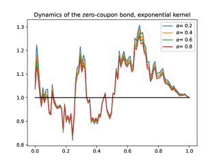
Figure 1. Dynamics of the zero-coupon bond in the Exponential kernel case.

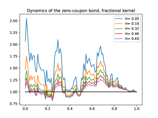
Figure 2. Dynamics of the zero-coupon bond in the Riemann-Liouville kernel case.

4.2. Impact of the roughness on convexity

We compare in Figures 3 and 4 the impact of the (roughness of the) kernel on the convexity adjustment. We consider a constant curve $\theta(\cdot)=6\%$ as well as $(t,\mathfrak{t}_{1},\mathfrak{t}_{2},tau)=(1,2,3,2)$. We note that, as $\alpha$ tends to zero in the exponential kernel case and as $H$ tends to $\frac{1}{2}$ in the Riemann-Liouville case, the convexity adjustments converge to the same value (as expected), approximately equal to $2.718$.

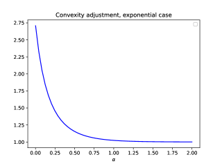
Figure 3. Impact of the exponential factor $\alpha$ on the convexity for the Exponential kernel from Section 2.3.1

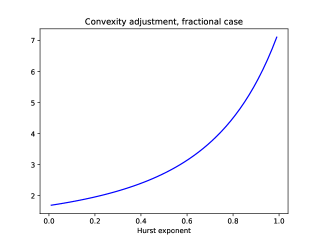
Figure 4. Impact of the Hurst exponent $H$ on the convexity for the power-law kernel from Section 2.3.2

References

- [1] E. Alòs, O. Mazet, and D. Nualart, Stochastic calculus with respect to Gaussian processes, The Annals of Probability, 29 (2001), pp. 766–801.
- [2] L. Andersen and V. Piterbarg, Interest Rate Modeling, Atlantic Financial Press, 2010.
- [3] A. Basse-O’Connor and S.-E. Graversen, Path and semimartingale properties of chaos processes, Stochastic processes and their applications, 120 (2010), pp. 522–540.
- [4] C. Bayer, P. Friz, and J. Gatheral, Pricing under rough volatility, Quantitative Finance, 16 (2016), pp. 887–904.
- [5] O. Bonesini, A. Jacquier, and A. Pannier, Rough volatility, path-dependent PDEs and weak rates of convergence. arXiv:2304.03042, 2023.
- [6] R. Brotherton-Ratcliffe and B. Iben, Yield curve applications of swap products, Schwartz, RJ, Smith, CW, Advanced Strategies in Financial Risk Management, New York Institute of Finance, New York, (1993), pp. 400–450.
- [7] O. El Euch, M. Fukasawa, and M. Rosenbaum, The microstructural foundations of leverage effect and rough volatility, Finance and Stochastics, 22 (2018), pp. 241–280.
- [8] B. Flesaker, Arbitrage free pricing of interest rate futures and forward contracts, The Journal of Futures Markets (1986-1998), 13 (1993), p. 77.
- [9] M. Fukasawa, Volatility has to be rough, Quantitative Finance, 21 (2021), pp. 1–8.
- [10] D. García-Lorite and R. Merino, Convexity adjustments à la Malliavin. arXiv:2304.13402, 2023.
- [11] J. Gatheral, T. Jaisson, and M. Rosenbaum, Volatility is rough, Quantitative Finance, 18 (2018), pp. 933–949.
- [12] A. Jacquier, A. Muguruza, and A. Pannier, Rough multifactor volatility for SPX and VIX options. arXiv:2112.14310, 2021.
- [13] A. Jacquier and M. Oumgari, Deep curve-dependent PDEs for affine rough volatility, SIAM Journal on Financial Mathematics, 14 (2023), pp. 353–382.
- [14] G. Kirikos and D. Novak, Convexity conundrums: Presenting a treatment of swap convexity in the hall-white framework, Risk Magazine, 10 (1997), pp. 60–61.
- [15] B. Øksendal, Stochastic differential equations, Springer, 2003.
- [16] A. Pelsser, Mathematical foundation of convexity correction, Quantitative Finance, 3 (2003), pp. 59–65.
- [17] P. Ritchken and L. Sankarasubramanian, Averaging and deferred payment yield agreements, The Journal of Futures Markets (1986-1998), 13 (1993), p. 23.
- [18] F. Russo and C. A. Tudor, On bifractional Brownian motion, Stochastic Processes and their applications, 116 (2006), pp. 830–856.
- [19] O. Vasicek, An equilibrium characterization of the term structure, Journal of Financial Economics, 5 (1977), pp. 177–188.