Magnetic fields & rotation periods of M dwarfs from SPIRou spectra

Abstract

We present near-infrared spectropolarimetric observations of a sample of 43 weakly- to moderately-active M dwarfs, carried with SPIRou at the Canada-France-Hawaii Telescope in the framework of the SPIRou Legacy Survey from early 2019 to mid 2022. We use the 6700 circularly polarised spectra collected for this sample to investigate the longitudinal magnetic field and its temporal variations for all sample stars, from which we diagnose, through quasi-periodic Gaussian process regression, the periodic modulation and longer-term fluctuations of the longitudinal field. We detect the large-scale field for 40 of our 43 sample stars, and infer a reliable or tentative rotation period for 38 of them, using a Bayesian framework to diagnose the confidence level at which each rotation period is detected. We find rotation periods ranging from 14 to over 60 d for the early-M dwarfs, and from 70 d to 200 d for most mid- and late-M dwarfs (potentially up to 430 d for one of them). We also find that the strength of the detected large-scale fields does not decrease with increasing period or Rossby number for the slowly rotating dwarfs of our sample as it does for higher-mass, more active stars, suggesting that these magnetic fields may be generated through a different dynamo regime than those of more rapidly rotating stars. We also show that the large-scale fields of most sample stars evolve on long timescales, with some of them globally switching sign as stars progress on their putative magnetic cycles.

1 Introduction

Magnetic fields of M dwarfs have triggered sustained interest since the first detection of a strong field at surface of the M3 dwarf AD Leo (Saar & Linsky, 1985). First diagnosed through the Zeeman broadening of unpolarized spectral lines, giving access to the small-scale field at the surface of the star, magnetic fields of M dwarfs were then detected through polarized Zeeman signatures in spectral lines (Donati et al., 2006a), yielding information on the large-scale field topology. Both quantities are now routinely monitored on a large sample of partly- to fully-convective M dwarfs, outlining how their fields change with stellar parameters such as mass, rotation period and age (Donati & Landstreet, 2009; Reiners, 2012; Kochukhov, 2021; Reiners et al., 2022), and what it implies in terms of the underlying dynamo processes amplifying and sustaining them in the convective envelopes or interiors of these stars (e.g., Shulyak et al., 2015).

With the detection of many planets and planetary systems around nearby M dwarfs over the last two decades (e.g., Bonfils et al., 2013; Gaidos et al., 2016), there is even more interest in investigating the magnetic fields of our low-mass stellar neighbours. Not only do these fields trigger all sorts of activity phenomena such as flares or surface brightness inhomogeneities and thereby induce different kinds of radial velocity (RV) perturbations (e.g., Reiners et al., 2010; Hébrard et al., 2014), but they can also generate star / planet interactions for close-in planets and potentially affect their orbital parameters (e.g., Strugarek et al., 2015), or even impact the habitability of rocky planets located in the habitable zones of their host stars (Vidotto et al., 2013).

Using spectropolarimetric observations, one can measure the longitudinal magnetic field of stars, i.e., the line-of-sight-projected component of the magnetic field vector averaged over the visible hemisphere of the star, noted $B_{\rm\ell}$, and its modulation with time if stars are monitored over a given time frame. For stars whose large-scale field is not symmetric with respect to the rotation axis, doing so gives access to the rotation period of stars, as first discovered in the context of chemically peculiar (Cp) stars (Babcock, 1949; Stibbs, 1950) then extensively used for all classes of magnetic stars (Landstreet, 1992; Donati & Landstreet, 2009). Time series of phase-resolved polarized Zeeman signatures of spectral lines can then be analysed with Principal Component Analysis (Lehmann & Donati, 2022), or inverted into maps of the large-scale magnetic field using tomographic techniques inspired from medical imaging (e.g., Semel, 1989; Donati et al., 2006b; Kochukhov, 2021).

Whereas rotation periods of active M dwarfs are often known from their photometric variability (Kiraga & Stepien, 2007), this is far less the case for weakly-active stars with presumably long rotation periods. Yet, estimating these rotation periods is essential, for instance to avoid confusing planetary RV signatures from those induced by activity. Carrying out velocimetric observations in the near-infrared (nIR) where the RV impact of activity is smaller obviously helps in this respect (e.g., Carmona et al., 2023). This is the same with spectropolarimetry as Zeeman signatures are comparatively larger in the nIR than in the optical for a given field topology and spectral line depth, making it especially interesting for studying magnetic fields and rotation periods of M dwarfs that are brightest in this spectral window.

In this paper, we concentrate on series of $B_{\rm\ell}$ measurements collected with SPIRou, the nIR spectropolarimeter (Donati et al., 2020) mounted at the Cassegrain focus of the Canada-France-Hawaii Telescope (CFHT) atop Maunakea, for a sample of 43 M dwarfs monitored in the context of the SPIRou Legacy Survey (SLS) over a time frame of 7 semesters (from 2019a to 2022a). This sample and the corresponding SPIRou raw frames are identical to those analysed by Fouqué et al. (2023) to find out the rotation periods of the sample stars from $B_{\rm\ell}$ measurements. In this new study however, everything else is different, from the data reduction to the modeling of the extracted spectra and Zeeman signatures. Being carried out with the same reference tools used to process and analyse extensive sets of ESPaDonS and NARVAL optical spectropolarimetric data (e.g., Morin et al., 2008; Hébrard et al., 2016), our study can thereby serve as a comparison point to double check the consistency of new results based on SPIRou data vs older ones derived from ESPaDOnS and NARVAL data, and to assess the agreement between results of various studies based on the same SPIRou data but reduced and analysed with a different set of tools (e.g., Fouqué et al., 2023).

After briefly outlining what our stellar sample and observations consist of (Sec. 2), we describe the $B_{\rm\ell}$ values we retrieve and whether the field is detected and variable with time (Sec. 3). We then detail the modeling of these time series to investigate whether and how reliably we detect the rotation periods of all sample stars (Sec. 4) and clarify the particular cases of a number of individual stars when needed (Sec. 5). We finally summarize and discuss in Sec. 6 the interest of our new results for our understanding of large-scale magnetic fields and dynamo action in slowly rotating M dwarfs.

Table 1: Stellar sample studied in this paper. For each star, columns 2 to 6 list the effective temperature $T_{\rm eff}$, the logarithmic gravity $\log g$, the metallicity ${\rm[M/H]}$, the mass $M_{\star}$ and radius $R_{\star}$ (from Cristofari et al., 2022), whereas columns 7 to 10 give the number of successful visits $n$ and the number of rejected spectra $r$, the LSD mask used (M0 or M3), the number of 2 km s^-1 pixels on which the LSD profiles were integrated to derive $B_{\rm\ell}$ values (see Eq. 1), and the average error bar on $B_{\rm\ell}$. Stars are ordered by decreasing $T_{\rm eff}$.

Star	$T_{\rm eff}$	$\log g$	${\rm[M/H]}$	$M_{\star}$	$R_{\star}$	$n/r$	mask	width	$\sigma_{B}$
	(K)			(${\rm M}_{\odot}$)	(${\rm R}_{\odot}$)			(pix)	(G)
Gl 338B	$3952\pm 30$	$4.71\pm 0.05$	$-0.08\pm 0.10$	$0.58\pm 0.02$	$0.609\pm 0.012$	50 / 0	M0	13	1.4
Gl 410	$3842\pm 31$	$4.87\pm 0.05$	$0.05\pm 0.10$	$0.55\pm 0.02$	$0.543\pm 0.009$	132 / 2	M0	19	4.4
Gl 846	$3833\pm 31$	$4.69\pm 0.05$	$0.07\pm 0.10$	$0.57\pm 0.02$	$0.568\pm 0.009$	201 / 1	M0	13	2.1
Gl 205	$3771\pm 31$	$4.70\pm 0.05$	$0.43\pm 0.10$	$0.58\pm 0.02$	$0.588\pm 0.010$	156 / 4	M0	13	1.0
Gl 880	$3702\pm 31$	$4.72\pm 0.05$	$0.26\pm 0.10$	$0.55\pm 0.02$	$0.563\pm 0.009$	168 / 0	M0	13	1.7
Gl 514	$3699\pm 31$	$4.74\pm 0.05$	$-0.07\pm 0.10$	$0.50\pm 0.02$	$0.497\pm 0.008$	167 / 10	M0	13	2.9
Gl 382	$3644\pm 31$	$4.75\pm 0.05$	$0.15\pm 0.10$	$0.51\pm 0.02$	$0.511\pm 0.009$	114 / 4	M0	13	2.4
Gl 412A	$3620\pm 31$	$4.79\pm 0.05$	$-0.42\pm 0.10$	$0.39\pm 0.02$	$0.391\pm 0.007$	165 / 8	M0	13	4.1
Gl 15A	$3611\pm 31$	$4.80\pm 0.05$	$-0.33\pm 0.10$	$0.39\pm 0.02$	$0.345\pm 0.015$	235 / 7	M0	13	2.7
Gl 411	$3589\pm 31$	$4.74\pm 0.05$	$-0.38\pm 0.10$	$0.39\pm 0.02$	$0.383\pm 0.008$	166 / 2	M3	13	2.0
Gl 752A	$3558\pm 31$	$4.69\pm 0.05$	$0.11\pm 0.10$	$0.47\pm 0.02$	$0.469\pm 0.008$	128 / 2	M3	13	2.4
Gl 48	$3529\pm 31$	$4.68\pm 0.05$	$0.08\pm 0.10$	$0.46\pm 0.02$	$0.469\pm 0.008$	190 / 3	M3	13	3.8
Gl 617B	$3525\pm 31$	$4.84\pm 0.06$	$0.20\pm 0.10$	$0.45\pm 0.02$	$0.460\pm 0.008$	144 / 6	M3	17	5.3
Gl 480	$3509\pm 31$	$4.88\pm 0.06$	$0.26\pm 0.10$	$0.45\pm 0.02$	$0.449\pm 0.008$	107 / 1	M3	13	3.9
Gl 436	$3508\pm 31$	$4.75\pm 0.05$	$0.03\pm 0.10$	$0.42\pm 0.02$	$0.425\pm 0.008$	92 / 0	M3	13	3.3
Gl 849	$3502\pm 31$	$4.88\pm 0.06$	$0.35\pm 0.10$	$0.46\pm 0.02$	$0.458\pm 0.008$	205 / 1	M3	13	3.6
Gl 408	$3487\pm 31$	$4.79\pm 0.05$	$-0.09\pm 0.10$	$0.38\pm 0.02$	$0.390\pm 0.007$	157 / 6	M3	21	7.8
Gl 687	$3475\pm 31$	$4.71\pm 0.05$	$0.01\pm 0.10$	$0.39\pm 0.02$	$0.414\pm 0.007$	212 / 8	M3	13	2.8
Gl 725A	$3470\pm 31$	$4.77\pm 0.06$	$-0.26\pm 0.10$	$0.33\pm 0.02$	$0.345\pm 0.006$	211 / 4	M3	15	4.2
Gl 317	$3421\pm 31$	$4.71\pm 0.06$	$0.23\pm 0.10$	$0.42\pm 0.02$	$0.423\pm 0.008$	77 / 2	M3	13	4.6
Gl 251	$3420\pm 31$	$4.71\pm 0.06$	$-0.01\pm 0.10$	$0.35\pm 0.02$	$0.365\pm 0.007$	178 / 3	M3	15	5.1
GJ 4063	$3419\pm 31$	$4.77\pm 0.06$	$0.42\pm 0.10$	$0.42\pm 0.02$	$0.422\pm 0.008$	219 / 3	M3	13	4.4
Gl 725B	$3379\pm 31$	$4.82\pm 0.06$	$-0.28\pm 0.10$	$0.25\pm 0.02$	$0.280\pm 0.005$	208 / 3	M3	13	5.0
PM J09553-2715	$3366\pm 31$	$4.76\pm 0.06$	$-0.03\pm 0.10$	$0.29\pm 0.02$	$0.302\pm 0.006$	76 / 3	M3	13	5.9
Gl 876	$3366\pm 31$	$4.80\pm 0.06$	$0.15\pm 0.10$	$0.33\pm 0.02$	$0.333\pm 0.006$	91 / 1	M3	13	3.5
GJ 1012	$3363\pm 31$	$4.66\pm 0.06$	$0.07\pm 0.10$	$0.35\pm 0.02$	$0.367\pm 0.007$	137 / 7	M3	13	6.3
GJ 4333	$3362\pm 31$	$4.72\pm 0.06$	$0.25\pm 0.10$	$0.37\pm 0.02$	$0.386\pm 0.008$	186 / 4	M3	13	5.2
Gl 445	$3356\pm 31$	$4.85\pm 0.06$	$-0.24\pm 0.10$	$0.24\pm 0.02$	$0.266\pm 0.005$	91 / 5	M3	13	7.2
GJ 1148	$3354\pm 31$	$4.70\pm 0.06$	$0.11\pm 0.10$	$0.34\pm 0.02$	$0.365\pm 0.007$	98 / 5	M3	13	6.1
PM J08402+3127	$3347\pm 31$	$4.76\pm 0.06$	$-0.08\pm 0.10$	$0.28\pm 0.02$	$0.299\pm 0.006$	130 / 5	M3	13	6.9
GJ 3378	$3326\pm 31$	$4.81\pm 0.06$	$-0.05\pm 0.10$	$0.26\pm 0.02$	$0.279\pm 0.005$	178 / 3	M3	13	6.2
GJ 1105	$3324\pm 31$	$4.63\pm 0.07$	$-0.04\pm 0.10$	$0.27\pm 0.02$	$0.283\pm 0.005$	167 / 2	M3	13	6.0
Gl 699	$3311\pm 31$	$5.11\pm 0.06$	$-0.37\pm 0.10$	$0.16\pm 0.02$	$0.185\pm 0.004$	247 / 3	M3	13	4.6
Gl 169.1A	$3307\pm 31$	$4.71\pm 0.06$	$0.13\pm 0.10$	$0.28\pm 0.02$	$0.292\pm 0.006$	172 / 7	M3	13	5.7
PM J21463+3813	$3305\pm 33$	$5.06\pm 0.08$	$-0.38\pm 0.10$	$0.18\pm 0.02$	$0.208\pm 0.004$	185 / 4	M3	13	10.1
Gl 15B	$3272\pm 31$	$4.89\pm 0.06$	$-0.42\pm 0.10$	$0.16\pm 0.02$	$0.182\pm 0.004$	179 / 6	M3	13	8.3
GJ 1289	$3238\pm 32$	$5.00\pm 0.07$	$0.05\pm 0.10$	$0.21\pm 0.02$	$0.233\pm 0.005$	204 / 9	M3	23	15.3
Gl 447	$3198\pm 31$	$4.82\pm 0.06$	$-0.13\pm 0.10$	$0.18\pm 0.02$	$0.201\pm 0.004$	57 / 0	M3	13	5.9
GJ 1151	$3178\pm 31$	$4.71\pm 0.06$	$-0.16\pm 0.10$	$0.17\pm 0.02$	$0.193\pm 0.004$	158 / 4	M3	13	7.9
GJ 1103	$3170\pm 31$	$4.67\pm 0.06$	$-0.03\pm 0.10$	$0.19\pm 0.02$	$0.224\pm 0.005$	60 / 9	M3	13	8.7
Gl 905	$3069\pm 31$	$4.78\pm 0.08$	$0.05\pm 0.11$	$0.15\pm 0.02$	$0.165\pm 0.004$	219 / 3	M3	13	6.8
GJ 1002	$2980\pm 33$	$4.70\pm 0.08$	$-0.33\pm 0.11$	$0.12\pm 0.02$	$0.139\pm 0.003$	140 / 6	M3	13	9.3
GJ 1286	$2961\pm 33$	$4.55\pm 0.12$	$-0.23\pm 0.10$	$0.12\pm 0.02$	$0.142\pm 0.004$	104 / 10	M3	13	10.0

2 SPIRou observations

In this paper, we focus on the 43 stars listed in Table 1, the same as in Fouqué et al. (2023), observed with SPIRou more than 50 times over the duration of the SLS (for a description of the whole sample, see Moutou et al., 2023). We recall that SPIRou collects nIR spectra of stars at a resolving power of 70 000, spanning a spectral window ranging from 0.95 to 2.50 $\mu$m ($Y$$J$$H$$K$ bands, with a small 2-nm gap at 2.438 $\mu$m, Donati et al., 2020). SPIRou is also a spectropolarimeter, capable of measuring polarization in spectral lines. It does so by carrying out, at each visit, a sequence of 4 sub-exposures in the pre-defined positions of the polarimeter quarter-wave Fresnel-rhomb retarders that can yield the requested polarization state with minimal errors. In this study, all stars were observed in circular polarization, leading to one Stokes $I$ (unpolarized) and one Stokes $V$ (circular polarization) spectrum per star and per visit; from the same data, we also compute a null polarization check called $N$, expected to yield a null signature when the polarimeter and reduction pipeline behave nominally (Donati et al., 1997).

As opposed to Fouqué et al. (2023) where the nominal SPIRou reduction package APERO (optimized for RV precision, Cook et al., 2022) was used, all data in this study were processed with the alternate package Libre-ESpRIT, i.e., the nominal ESPaDOnS reduction pipeline (Donati et al., 1997) adapted for SPIRou data (Donati et al., 2020). Optimized for polarimetry and checked against magnetic standard (Cp) stars, Libre-ESpRIT can be considered as a reference in this respect (Donati et al., 1997; Donati et al., 2020). The main differences between the two pipelines are the way the spectra of both science channels (i.e., both orthogonal polarization states) are extracted from the raw frames of each sub-exposure on the one hand, and how Stokes $V$ spectra are derived from those of both science channels and all sub-exposures on the other. We do not expect significant differences between both pipelines for these steps, that were cross-checked on spectra of a few reference stars (e.g., AD Leo), except on how error bars are propagated from the raw frames to the Stokes $V$ spectra.

We then applied our version of Least-Squares Deconvolution (LSD, Donati et al., 1997) to all reduced Stokes $I$, $V$, and $N$ spectra of all stars, in contrast to Fouqué et al. (2023) who used a different LSD implementation. In our case, we carried out LSD using 2 main line masks, an M0 mask for stars whose effective temperature $T_{\rm eff}$ is larger than 3600 K and an M3 mask for all others. In these masks, that we constructed using VALD-3 (Ryabchikova et al., 2015) assuming a logarithmic gravity of $\hbox{$\log g$}=5$ and a solar metallicity ${\rm[M/H]}$, we only use atomic lines whose relative depth with respect to the continuum (including microturbulence only) is larger than 10 per cent, and with known magnetic sensitivity (Landé factor). We end up exploiting about 800 atomic lines for the M0 mask, and 575 lines for the M3 mask. We also tried incorporating weaker lines in the mask (down to relative depths of 7, 5 or 3 percent), but found that the 10 per cent threshold in relative line depth gives the best results in terms of reliability of the Zeeman detections. For each star, the few epochs for which LSD Stokes $I$ profiles were of much lower quality than the typical one (e.g., as a result of poor weather) were rejected from our data set. This second step is also different between the two studies, with Fouqué et al. (2023) using not only a different implementation of LSD, but also different line masks and different thresholds on line strengths. To our knowledge, the alternate LSD tools used by Fouqué et al. (2023) have not been extensively cross-checked with ours, and may generate potential differences between the two approaches.

For each set of LSD Stokes $I$, $V$ and $N$ profiles associated with one visit, we compute $B_{\rm\ell}$, its $N$ equivalent and the corresponding error bars following Donati et al. (1997), i.e., from the first moment of the $V(v)$ (and $N(v)$) profile normalised by the equivalent with of the $I(v)$ profile, (both integrated over velocity $v$):

$$\hbox{$B_{\rm\ell}$}=-2.14\times 10^{11}\frac{\int vV(v)\mathrm{d}v}{\lambda gc\int[1-I(v)]\mathrm{d}v}$$ (1)

with $B_{\rm\ell}$ in G, $v$ and $c$ (the speed of light) in km s^-1, and where $g$ and $\lambda$ (in nm) refer to the equivalent Landé factor and wavelength of the resulting Stokes $I$, $V$ (and $N$) LSD profiles. Error bars are derived analytically from Eq. 1 and the noise in LSD profiles, themselves computed by propagating the photon noise in the $I$, $V$ and $N$ spectra (Donati et al., 1997). The integration is carried out over a window centred on the median stellar RV, of width $\pm 13$ km s^-1 about the center for most stars, except for a few whose Zeeman signatures are stronger and / or wider than average and for which this interval was widened to $\pm 15$ km s^-1 (Gl 725A and Gl 251), $\pm 17$ km s^-1 (Gl 617B), $\pm 19$ km s^-1 (Gl 410), $\pm 21$ km s^-1 (Gl 408) and up to $\pm 23$ km s^-1 (GJ 1289). Keeping this window as narrow as possible is indeed key for minimizing the error bar on $B_{\rm\ell}$ (denoted $\sigma_{B}$) while retaining all information about the longitudinal field. In practice, we looked at the time averaged absolute value of the Stokes $V$ profiles for each star, and verified that no signal is detected above the continuum photon noise outside of the selected interval; we also checked that the standard deviation of Stokes $V$ profiles for each star shows no signal outside of this window. We find that the average $\sigma_{B}$ per star varies from 1.0 to 15.3 G (depending on the stellar magnitude and spectral type) in our observations, with a median of 4.4 G (see Table 1). This third step is also slightly different in Fouqué et al. (2023), where integration is carried out on a significantly wider window. However, we do not expect major discrepancies from such differences, mostly larger error bars on $B_{\rm\ell}$ values as a result of the wider integration window.

Table 2: Statistics on the $B_{\rm\ell}$ values from the LSD Stokes $V$ and $N$ profiles, for each star of our sample. Columns 2 to 5, computed from LSD Stokes $V$ profiles, respectively list the weighted-average and standard deviation of $B_{\rm\ell}$, the average error bar $\sigma_{B}$, the reduced chi square $\chi^{2}_{\rm r}$ of $B_{\rm\ell}$ and $B_{\rm\ell}$$-$<$B_{\rm\ell}$> (where <> notes the weighted average), and the detection status (DS) of $B_{\rm\ell}$ and $B_{\rm\ell}$$-$<$B_{\rm\ell}$> (with DD, MD and ND standing for Definite Detection, Marginal Detection and No Detection, see text for how these cases are defined). Columns 6 to 9 give the same quantities, but derived from the LSD $N$ profiles. The last column recalls the number of visits $n$ for each star.

	Stokes $V$					$N$
Star	<$B_{\rm\ell}$> / RMS	$\sigma_{B}$	$\chi^{2}_{\rm r}$	DS		<$B_{\rm\ell}$> / RMS	$\sigma_{B}$	$\chi^{2}_{\rm r}$	DS		$n$
	(G)	(G)	$B_{\rm\ell}$ / $B_{\rm\ell}$$-$<$B_{\rm\ell}$>			(G)	(G)	$B_{\rm\ell}$ / $B_{\rm\ell}$$-$<$B_{\rm\ell}$>
Gl 338B	-3.8 / 4.3	1.4	9.93 / 2.13	DD / DD		-0.1 / 1.6	1.4	1.30 / 1.30	ND / ND		50
Gl 410	-0.1 / 16.7	4.4	14.20 / 14.20	DD / DD		-0.3 / 4.2	4.5	0.89 / 0.89	ND / ND		132
Gl 846	0.0 / 3.4	2.1	2.70 / 2.70	DD / DD		0.3 / 2.2	2.1	1.07 / 1.05	ND / ND		201
Gl 205	1.5 / 3.2	1.0	10.60 / 8.19	DD / DD		-0.1 / 1.0	1.0	1.07 / 1.05	ND / ND		156
Gl 880	0.3 / 4.2	1.7	6.25 / 6.21	DD / DD		-0.1 / 1.9	1.7	1.20 / 1.19	ND / ND		168
Gl 514	-2.5 / 5.3	2.9	3.31 / 2.57	DD / DD		0.0 / 2.9	2.9	0.96 / 0.96	ND / ND		167
Gl 382	-1.3 / 4.8	2.4	3.90 / 3.63	DD / DD		-0.1 / 2.5	2.4	1.04 / 1.04	ND / ND		114
Gl 412A	7.0 / 8.9	4.1	4.77 / 1.80	DD / DD		-0.1 / 4.0	4.1	0.92 / 0.92	ND / ND		165
Gl 15A	0.1 / 3.4	2.7	1.59 / 1.59	DD / DD		-0.1 / 3.0	2.8	1.20 / 1.20	ND / ND		235
Gl 411	2.2 / 3.3	2.0	2.69 / 1.49	DD / MD		0.2 / 2.4	2.1	1.30 / 1.29	ND / ND		166
Gl 752A	0.2 / 3.7	2.4	2.31 / 2.30	DD / DD		0.0 / 2.4	2.5	0.98 / 0.98	ND / ND		128
Gl 48	-2.7 / 5.9	3.8	2.42 / 1.90	DD / DD		0.3 / 3.7	3.9	0.93 / 0.93	ND / ND		190
Gl 617B	12.6 / 14.4	5.3	7.47 / 1.85	DD / DD		0.4 / 5.8	5.4	1.18 / 1.17	ND / ND		144
Gl 480	1.0 / 5.8	3.9	2.23 / 2.16	DD / DD		0.1 / 3.7	3.9	0.89 / 0.89	ND / ND		107
Gl 436	-5.1 / 6.5	3.3	4.03 / 1.63	DD / MD		0.3 / 2.7	3.3	0.66 / 0.65	ND / ND		92
Gl 849	2.1 / 5.5	3.6	2.33 / 1.98	DD / DD		0.6 / 3.4	3.7	0.86 / 0.83	ND / ND		205
Gl 408	-29.9 / 29.0	7.8	15.94 / 1.37	DD / ND		0.7 / 7.8	7.9	0.97 / 0.96	ND / ND		157
Gl 687	0.7 / 4.4	2.8	2.47 / 2.41	DD / DD		-0.0 / 2.8	2.8	0.97 / 0.97	ND / ND		212
Gl 725A	-7.6 / 9.2	4.2	4.74 / 1.47	DD / MD		-0.1 / 4.5	4.3	1.11 / 1.11	ND / ND		211
Gl 317	-1.9 / 6.2	4.6	1.81 / 1.65	MD / MD		0.6 / 4.6	4.7	0.99 / 0.97	ND / ND		77
Gl 251	9.3 / 11.0	5.1	4.65 / 1.39	DD / MD		-0.3 / 4.9	5.2	0.91 / 0.90	ND / ND		178
GJ 4063	7.3 / 8.6	4.4	3.92 / 1.17	DD / ND		0.4 / 4.2	4.4	0.91 / 0.90	ND / ND		219
Gl 725B	-2.5 / 6.0	5.0	1.49 / 1.24	DD / ND		0.6 / 5.0	5.0	0.99 / 0.98	ND / ND		208
PM J09553-2715	8.2 / 10.3	5.9	3.52 / 1.57	DD / ND		-0.3 / 5.5	5.9	0.86 / 0.86	ND / ND		76
Gl 876	1.7 / 7.3	3.5	4.37 / 4.13	DD / DD		0.8 / 3.6	3.5	1.03 / 0.97	ND / ND		91
GJ 1012	1.9 / 6.7	6.3	1.14 / 1.04	ND / ND		0.3 / 6.1	6.3	0.94 / 0.94	ND / ND		137
GJ 4333	2.0 / 8.0	5.2	2.36 / 2.21	DD / DD		0.3 / 5.1	5.3	0.96 / 0.95	ND / ND		186
Gl 445	-0.1 / 7.3	7.2	1.02 / 1.02	ND / ND		-0.0 / 7.4	7.3	1.04 / 1.04	ND / ND		91
GJ 1148	-5.5 / 8.4	6.1	2.01 / 1.19	DD / ND		-0.7 / 6.0	6.1	0.98 / 0.96	ND / ND		98
PM J08402+3127	12.9 / 17.5	6.9	6.93 / 3.41	DD / DD		-0.3 / 7.6	6.9	1.19 / 1.19	ND / ND		130
GJ 3378	5.3 / 9.2	6.2	2.26 / 1.52	DD / MD		0.8 / 5.8	6.2	0.87 / 0.85	ND / ND		178
GJ 1105	-0.2 / 6.1	6.0	1.01 / 1.01	ND / ND		0.6 / 6.1	6.1	0.99 / 0.98	ND / ND		167
Gl 699	1.6 / 6.9	4.6	2.28 / 2.16	DD / DD		0.6 / 5.1	4.7	1.18 / 1.17	ND / ND		247
Gl 169.1A	-1.8 / 7.0	5.7	1.49 / 1.40	MD / MD		0.9 / 5.9	5.8	1.05 / 1.02	ND / ND		172
PM J21463+3813	0.7 / 11.1	10.1	1.22 / 1.22	ND / ND		-0.0 / 10.5	10.2	1.07 / 1.07	ND / ND		185
Gl 15B	-0.4 / 10.8	8.3	1.70 / 1.69	DD / DD		0.6 / 8.0	8.3	0.93 / 0.92	ND / ND		179
GJ 1289	47.4 / 40.6	15.3	19.68 / 10.12	DD / DD		0.4 / 14.8	15.4	0.92 / 0.92	ND / ND		204
Gl 447	10.1 / 12.0	5.9	5.20 / 2.31	DD / DD		-1.0 / 6.0	6.0	1.01 / 0.99	ND / ND		57
GJ 1151	1.7 / 16.8	7.9	4.60 / 4.55	DD / DD		1.0 / 7.8	7.9	0.97 / 0.96	ND / ND		158
GJ 1103	4.0 / 10.2	8.7	1.72 / 1.50	MD / ND		-0.2 / 8.7	8.8	0.98 / 0.98	ND / ND		60
Gl 905	-6.7 / 15.6	6.8	5.37 / 4.38	DD / DD		-0.1 / 7.1	6.8	1.07 / 1.07	ND / ND		219
GJ 1002	-0.5 / 10.0	9.3	1.15 / 1.14	ND / ND		0.1 / 9.2	9.4	0.95 / 0.95	ND / ND		140
GJ 1286	15.4 / 18.2	10.0	5.53 / 3.14	DD / DD		-1.7 / 8.7	10.1	0.76 / 0.74	ND / ND		104

3 Longitudinal field and its temporal variations

We start by carrying out a statistical analysis on the series of $B_{\rm\ell}$ values for each star, computed from both LSD Stokes $V$ and $N$ profiles. We compute in particular the reduced chi squares $\chi^{2}_{\rm r}$ of both $B_{\rm\ell}$ and $B_{\rm\ell}$$-$<$B_{\rm\ell}$> series (where <> notes the weighted average over all epochs). Whereas the former indicates whether the longitudinal field is significantly different from zero, i.e., is detected, the latter informs on whether $B_{\rm\ell}$ fluctuates about its mean value by more than what the estimated error bars allow, i.e., that $B_{\rm\ell}$ is variable with time. Following Donati et al. (1997), we use the $\chi^{2}$ probability function (Press et al., 1992) to diagnose a detection, taking $n$ as the number of degrees of freedom. We consider that we can claim a definite detection (DD) if the false-alarm probability (FAP) is $<10^{-5}$, a marginal detection (MD) if the FAP is $<10^{-3}$, and that we have no detection (ND) otherwise. All $\chi^{2}_{\rm r}$ values are listed in Table 2, along with the corresponding Detection Status (DS). We also include in Table 2 the weighted average and standard deviations of $B_{\rm\ell}$ values, as well as the average error bar $\sigma_{B}$.

For all stars but 5 (namely GJ 1012, GJ 1105, Gl 445, PM J21463+3813 and GJ 1002), we obtain either a clear detection (35 stars) or a marginal detection (3 stars, Gl 317, Gl 169.1A and GJ 1103) of the longitudinal field. For the 5 stars with no detection, one can check in particular that <$B_{\rm\ell}$> is close to zero (within $\sigma_{B}$) and that the standard deviation of $B_{\rm\ell}$ is similar to $\sigma_{B}$. As detailed in Sec. 4, $B_{\rm\ell}$ seems to be detected for the last 2 of these 5 stars (PM J21463+3813 and GJ 1002) even though our statistical test conclude to a ND. It suggests that our error bars on $B_{\rm\ell}$ are slightly overestimated for a few of our targets, rendering our detection criterion a bit too stringent in such cases.

Out of the 38 stars where $B_{\rm\ell}$ is either clearly or marginally detected, 5 of them (GJ 4063, GJ 1148, PM J09553-2715, Gl 725B, GJ 1103) are diagnosed as showing no temporal variations of $B_{\rm\ell}$, whereas 5 (Gl 411, Gl 436, Gl 317, GJ 3378, Gl 169.1A) are identified as having a marginally variable $B_{\rm\ell}$. Once again, we will see later in the paper (Sec. 4) that 4 of the 5 stars whose $B_{\rm\ell}$ is listed as non variable are in fact found to show either clear or probable periodic $B_{\rm\ell}$ fluctuations, presumably for the same reason as that mentioned previously, i.e., that our detection criterion is too stringent at times. Only GJ 1148 ends up showing no $B_{\rm\ell}$ variations despite the large-scale field being clearly detected, possibly because the magnetic topology is almost perfectly axisymmetric or the star is seen almost exactly pole-on. Most of our targets thus show clear $B_{\rm\ell}$ detections and temporal variations, in particular GJ 1289, Gl 410, Gl 205, Gl 880, GJ 1151, Gl 905 and Gl 876 for which the $\chi^{2}_{\rm r}$ of $B_{\rm\ell}$$-$<$B_{\rm\ell}$> is larger than 4 and up to 16.6.

We finally note that $B_{\rm\ell}$ values derived from LSD $N$ profiles (columns 6 to 9 of Table 2) are all consistent with 0, with standard deviations equal to $\sigma_{B}$ and $\chi^{2}_{\rm r}$ equal to $1.00\pm 0.12$ on average over the sample of 43 stars. We note that $\chi^{2}_{\rm r}$ ranges from 0.7 to 1.3, reflecting mostly statistical photon noise fluctuations; moreover, the weighted-average <$B_{\rm\ell}$> is always very close to 0, causing the $\chi^{2}_{\rm r}$ associated with $B_{\rm\ell}$ and $B_{\rm\ell}$$-$<$B_{\rm\ell}$> to be almost identical for all stars. This is what we expect if the SPIRou polarimeter and the Libre-ESpRIT reduction package are working nominally regarding polarimetry, with no spurious signatures showing up in the null polarization check down to the photon noise level.

By comparing <$B_{\rm\ell}$> and $\sigma_{B}$ values in Table 2 to their equivalents in Fouqué et al. (2023), we see that both our $B_{\rm\ell}$ values and error bars are smaller than those of Fouqué et al. (2023) by a factor of 2$-$3. This is most obvious for stars where |<$B_{\rm\ell}$>| is larger than 10 G, but it is also the case for other stars with weaker fields. As Stokes $I$ and $V$ profiles spectra derived by Libre-ESpRIT and APERO apparently yield, for a few stars, consistent LSD profiles when the same LSD code (the one used here) is applied to both, we suspect that the discrepancy mentioned above mostly reflects differences in the LSD implementation used by Fouqué et al. (2023), i.e., in the step referred to as step 2 of our description of how SPIRou data were analyzed (see Sec. 2), and to a lesser extent in the way their $B_{\rm\ell}$ values were derived from LSD profiles (step 3). The origin of this difference is currently being investigated.

4 Periodicity of the $B_{\rm\ell}$ variations

To investigate whether the temporal variability of $B_{\rm\ell}$ is periodic, a standard Fourier analysis is not ideal for these mildly to weakly active M dwarfs, where $B_{\rm\ell}$ is expected to evolve on a timescale of the same order of magnitude as the rotation period itself. We therefore use instead Gaussian process regression (GPR) to the $B_{\rm\ell}$ data, with a quasi-periodic (QP) kernel whose covariance function $c(t,t^{\prime})$ is given by

$$c(t,t^{\prime})=\theta_{1}^{2}\exp\left(-\frac{(t-t^{\prime})^{2}}{2\theta_{3}^{2}}-\frac{\sin^{2}\left(\frac{\pi(t-t^{\prime})}{\theta_{2}}\right)}{2\theta_{4}^{2}}\right)$$ (2)

where $\theta_{1}$ is the amplitude (in G) of the Gaussian Process (GP), $\theta_{2}$ its recurrence period (i.e., $P_{\rm rot}$, in d), $\theta_{3}$ the timescale (in d) on which $B_{\rm\ell}$ evolves, and $\theta_{4}$ a smoothing parameter setting the level of harmonic complexity. Although our error bars on $B_{\rm\ell}$ are slightly overestimated (see Sec. 3), we nonetheless introduce a fifth hyper-parameter $\theta_{5}$ setting the amount of additional white noise potentially required by GPR (e.g., as a result of short-term intrinsic variability) to achieve the fit to the $B_{\rm\ell}$ values (denoted $y$) that maximizes likelihood $\mathcal{L}$, defined as:

$$2\log\mathcal{L}=-n\log(2\pi)-\log|C+\Sigma+S|-y^{T}(C+\Sigma+S)^{-1}y$$ (3)

where $C$ is the covariance matrix for our observation epochs, $\Sigma$ the diagonal variance matrix associated with $B_{\rm\ell}$, and $S=\theta_{5}^{2}I$ the contribution of the additional white noise ($I$ being the identity matrix). Coupled to a MCMC run to explore the parameter domain, one can find out the optimal set of hyper parameters and corresponding posterior distributions.

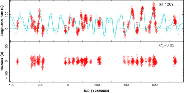
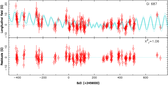
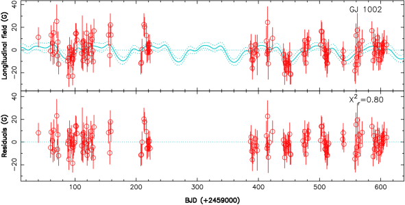
Figure 1: QP GPR fit and error bars (full and dotted cyan curves) of the $B_{\rm\ell}$ data (red open symbols with error bars) for GJ 1289 (top), Gl 687 (middle) and GJ 1002 (bottom). The corresponding $\Delta\log\mathcal{L}_{M}$ are respectively equal to 168.5 (the highest of the whole sample), 34.6 and 7.2, indicating a clear detection of the QP $B_{\rm\ell}$ modulation in the first 2 cases and a marginal detection in the third case (see Table 3).

Table 3: Results of the QP GPR applied to the $B_{\rm\ell}$ time series of our sample stars. Columns 2 lists the recovered period whenever detected, whereas columns 3 to 6 give the values of the 4 other hyper-parameters (with some fixed in a few cases). The achieved $\chi^{2}_{\rm r}$, RMS, $\Delta\log\mathcal{L}_{M}$ with respect to a model with no modulation, and the detection status of the periodic modulation are mentioned in columns 7 to 10. In column 7, we also mention in parenthesis the $\chi^{2}_{\rm r}$ for the GPR fit of the long-term $B_{\rm\ell}$ variations only, to emphasize how much it changes with respect to that of the main GPR fit.

Star	$P_{\rm rot}$	GP ampl.	Evol. timescale	Smoothing	White noise	$\chi^{2}_{\rm r}$	RMS	$\Delta\log\mathcal{L}_{M}$	DS
	$\theta_{2}$ (d)	$\theta_{1}$ (G)	$\theta_{3}$ (d)	$\theta_{4}$	$\theta_{5}$ (G)		(G)
Gl 338B	$42.2\pm 4.1$	$2.1^{+1.0}_{-0.7}$	$120$	$0.99\pm 0.59$	$0.6^{+0.4}_{-0.2}$	0.79 (1.97)	1.2	7.2	MD
Gl 410	$13.91\pm 0.09$	$17.2^{+2.8}_{-2.4}$	$59^{+9}_{-8}$	$0.48\pm 0.06$	$2.2^{+1.3}_{-0.8}$	0.71 (14.20)	3.7	85.0	DD
Gl 846	$21.84\pm 0.14$	$3.0^{+0.4}_{-0.4}$	$70^{+15}_{-12}$	$0.31\pm 0.04$	$0.4^{+0.3}_{-0.2}$	0.60 (2.70)	1.6	58.6	DD
Gl 205	$34.58\pm 0.46$	$2.9^{+0.4}_{-0.4}$	$53^{+11}_{-9}$	$0.37\pm 0.05$	$0.3^{+0.2}_{-0.1}$	0.69 (6.94)	0.8	85.5	DD
Gl 880	$37.21\pm 0.30$	$4.4^{+0.8}_{-0.6}$	$113^{+21}_{-18}$	$0.41\pm 0.06$	$0.4^{+0.3}_{-0.2}$	0.67 (5.51)	1.4	94.8	DD
Gl 514	$30.32\pm 0.21$	$4.0^{+1.4}_{-1.0}$	$300$	$0.60\pm 0.23$	$1.5^{+0.5}_{-0.4}$	1.14 (2.05)	3.1	29.0	DD
Gl 382	$21.91\pm 0.16$	$4.2^{+0.8}_{-0.7}$	$131^{+50}_{-36}$	$0.35\pm 0.07$	$0.8^{+0.6}_{-0.3}$	0.69 (3.63)	2.0	37.5	DD
Gl 412A	$36.9\pm 2.5$	$4.5^{+1.2}_{-1.0}$	$78^{+28}_{-21}$	$1.22\pm 0.58$	$1.2^{+0.8}_{-0.5}$	0.84 (1.33)	3.7	14.6	DD
Gl 15A	$43.26\pm 0.36$	$3.6^{+1.3}_{-1.0}$	$300$	$0.78\pm 0.26$	$1.0^{+0.5}_{-0.3}$	1.02 (1.41)	2.7	22.1	DD
Gl 411	$427\pm 34$	$1.3^{+0.4}_{-0.3}$	$300$	$0.24\pm 0.14$	$0.7^{+0.4}_{-0.3}$	0.95 (1.21)	2.0	11.9	DD
Gl 752A	$45.0\pm 4.2$	$2.8^{+0.7}_{-0.5}$	$63^{+27}_{-19}$	$0.51\pm 0.16$	$0.8^{+0.6}_{-0.3}$	0.90 (2.31)	2.3	19.0	DD
Gl 48	$52.1\pm 1.9$	$4.4^{+1.0}_{-0.8}$	$61^{+20}_{-15}$	$0.47\pm 0.17$	$1.0^{+0.7}_{-0.4}$	0.80 (1.90)	3.4	32.6	DD
Gl 617B	$40.4\pm 3.0$	$5.4^{+1.3}_{-1.0}$	$69^{+35}_{-23}$	$0.60\pm 0.22$	$1.7^{+1.1}_{-0.7}$	0.86 (1.56)	4.9	17.7	DD
Gl 480	$25.00\pm 0.24$	$6.6^{+3.5}_{-2.3}$	$300$	$1.16\pm 0.57$	$2.5^{+0.8}_{-0.6}$	1.26 (1.75)	4.4	9.7	MD
Gl 436	$48\pm 13$	$1.7^{+1.6}_{-0.8}$	$149^{+106}_{-62}$	$0.82\pm 0.78$	$1.3^{+1.0}_{-0.6}$	0.90 (1.63)	3.1	1.6	ND
Gl 849	$41.76\pm 0.61$	$4.8^{+1.5}_{-1.1}$	$209^{+58}_{-45}$	$0.47\pm 0.13$	$1.0^{+0.7}_{-0.4}$	0.89 (1.97)	3.4	39.0	DD
Gl 408	$171.0\pm 8.4$	$6.3^{+1.5}_{-1.2}$	$200$	$0.21\pm 0.10$	$1.5^{+1.2}_{-0.7}$	0.66 (1.16)	6.3	16.5	DD
Gl 687	$56.69\pm 0.56$	$5.9^{+2.0}_{-1.5}$	$300$	$0.78\pm 0.25$	$1.2^{+0.5}_{-0.3}$	1.06 (1.83)	2.9	34.6	DD
Gl 725A	$103.1\pm 6.1$	$3.4^{+0.7}_{-0.6}$	$86^{+51}_{-32}$	$0.32\pm 0.10$	$0.8^{+0.7}_{-0.4}$	0.78 (1.47)	3.7	24.1	DD
Gl 317	$39.0\pm 3.8$	$5.6^{+2.4}_{-1.7}$	$107^{+70}_{-42}$	$1.68\pm 0.70$	$1.3^{+1.0}_{-0.6}$	0.75 (1.04)	4.0	7.2	MD
Gl 251	$108.0\pm 2.2$	$4.0^{+1.2}_{-0.9}$	$300$	$0.30\pm 0.12$	$1.2^{+0.9}_{-0.5}$	0.83 (1.39)	4.7	15.3	DD
GJ 4063	$40.7\pm 3.5$	$2.7^{+1.0}_{-0.7}$	$93^{+42}_{-29}$	$1.17\pm 0.69$	$1.0^{+0.7}_{-0.4}$	0.84 (1.03)	4.0	7.9	MD
Gl 725B	$135\pm 15$	$3.2^{+0.9}_{-0.7}$	$122^{+81}_{-49}$	$0.52\pm 0.25$	$1.0^{+0.8}_{-0.4}$	0.89 (1.20)	4.7	12.9	DD
PM J09553-2715	$73.0\pm 3.5$	$7.4^{+5.1}_{-3.0}$	$300$	$0.81\pm 0.60$	$2.0^{+1.3}_{-0.8}$	0.85 (1.57)	5.4	6.8	MD
Gl 876	$83.7\pm 2.9$	$6.9^{+2.0}_{-1.6}$	$201^{+89}_{-62}$	$0.40\pm 0.13$	$1.1^{+0.9}_{-0.5}$	0.70 (3.15)	2.9	36.7	DD
GJ 1012		$2.3^{+2.6}_{-1.2}$	$300$	$1.00$	$1.6^{+1.2}_{-0.7}$	0.92 (1.04)	6.0	-4.0	ND
GJ 4333	$71.0\pm 1.5$	$6.6^{+1.4}_{-1.2}$	$150^{+52}_{-39}$	$0.37\pm 0.08$	$1.1^{+0.9}_{-0.5}$	0.77 (2.21)	4.6	49.8	DD
Gl 445		$1.4^{+1.5}_{-0.7}$	$300$	$1.00$	$2.2^{+1.5}_{-0.9}$	1.02 (1.02)	7.3	-2.2	ND
GJ 1148		$2.7^{+1.7}_{-1.0}$	$300$	$1.00$	$1.9^{+1.4}_{-0.8}$	1.04 (1.11)	6.2	1.8	ND
PM J08402+3127	$89.5\pm 8.0$	$14.0^{+4.2}_{-3.2}$	$219^{+58}_{-46}$	$1.50$	$1.7^{+1.3}_{-0.7}$	0.87 (1.13)	6.4	7.6	MD
GJ 3378	$95.1\pm 2.3$	$4.9^{+1.6}_{-1.2}$	$300$	$0.44\pm 0.21$	$1.7^{+1.3}_{-0.7}$	0.92 (1.39)	5.9	22.8	DD
GJ 1105		$2.1^{+2.1}_{-1.1}$	$300$	$1.00$	$1.4^{+1.1}_{-0.6}$	0.93 (1.01)	5.8	-3.9	ND
Gl 699	$136\pm 13$	$5.6^{+0.8}_{-0.7}$	$100$	$0.40$	$1.5^{+0.8}_{-0.5}$	0.95 (1.65)	4.5	44.5	DD
Gl 169.1A	$92.3\pm 3.6$	$5.6^{+2.6}_{-1.8}$	$300$	$1.08\pm 0.53$	$1.6^{+1.1}_{-0.6}$	0.91 (1.20)	5.5	12.7	DD
PM J21463+3813	$93.9\pm 3.4$	$7.7^{+2.8}_{-2.0}$	$300$	$0.51\pm 0.37$	$2.1^{+1.7}_{-0.9}$	0.82 (1.14)	9.1	14.2	DD
Gl 15B	$113.3\pm 4.3$	$10.5^{+5.0}_{-3.4}$	$250^{+83}_{-62}$	$0.79\pm 0.39$	$2.4^{+1.6}_{-1.0}$	0.92 (1.50)	8.0	23.8	DD
GJ 1289	$73.66\pm 0.92$	$53.2^{+12.4}_{-10.1}$	$152^{+32}_{-27}$	$0.48\pm 0.09$	$4.2^{+2.7}_{-1.6}$	0.82 (9.19)	13.9	168.5	DD
Gl 447	$24.1\pm 3.7$	$11.1^{+5.8}_{-3.8}$	$74^{+48}_{-29}$	$1.42\pm 0.69$	$2.3^{+1.5}_{-0.9}$	0.85 (1.31)	5.4	7.5	MD
GJ 1151	$175.6\pm 4.9$	$14.9^{+4.2}_{-3.3}$	$300$	$0.43\pm 0.14$	$1.6^{+1.3}_{-0.7}$	0.72 (1.85)	6.7	75.2	DD
GJ 1103	$142.6\pm 9.6$	$8.3^{+4.1}_{-2.7}$	$300$	$0.51\pm 0.29$	$2.6^{+2.1}_{-1.2}$	0.79 (1.50)	7.7	9.1	MD
Gl 905	$114.3\pm 2.8$	$13.3^{+2.5}_{-2.1}$	$129^{+25}_{-21}$	$0.43\pm 0.09$	$1.7^{+1.2}_{-0.7}$	0.84 (2.86)	6.2	94.5	DD
GJ 1002	$89.8\pm 2.8$	$8.3^{+5.0}_{-3.1}$	$300$	$0.96\pm 0.66$	$2.1^{+1.7}_{-0.9}$	0.80 (1.14)	8.3	7.2	MD
GJ 1286	$178\pm 15$	$16.7^{+4.6}_{-3.6}$	$300$	$0.29\pm 0.09$	$4.6^{+2.6}_{-1.6}$	1.02 (2.86)	10.1	28.2	DD

As in Donati et al. (2023), we use modified Jeffreys priors for $\theta_{1}$ (GP amplitude) and $\theta_{5}$ (white noise), with a knee set to $\sigma_{B}$, and a uniform prior for $\theta_{4}$ (smoothing parameter) in the range [0,3]. For $\theta_{3}$ (evolution timescale), we start with a log Gaussian prior centred on 150 d and a standard deviation of a factor of 3, then recenter it on the derived value in a second step (keeping the same standard deviation). Finally, for the rotation period ($\theta_{2}$, handled in linear space), we start with a uniform prior in the range [10,500] d, then change it to a Gaussian prior on each of the (potentially multiple) regions of maximum likelihood (with a standard deviation equal to 25% of the most probable local period), and ultimately select the period featuring the highest likelihood.

We start with a first MCMC run where all parameters are free to vary. In a few cases where the temporal variations of $B_{\rm\ell}$ are weak, we choose to fix $\theta_{4}$ to 1.0 or 1.5, to obtain a smooth fit to the $B_{\rm\ell}$ data. If $\theta_{3}$ reaches 300 d or more, suggesting that $B_{\rm\ell}$ evolves slowly from one year to the next, we fix it to this value. In one case where the data are sparse (Gl 338B), we fix $\theta_{3}$ to its optimal value (120 d). In another one where the $B_{\rm\ell}$ fluctuations are complex and varying rapidly (Gl 699), we have to fix $\theta_{4}$ to its optimal value (0.4) and $\theta_{3}$ to 100 d to ensure the latter does not get much smaller than the rotation period (which would prevent QP GPR to safely identify periodicity).

To estimate the confidence level in the derived rotation period, we compare the results of this MCMC run with with those of another model where only the amplitude of the long-term $B_{\rm\ell}$ variations is adjusted (by arbitrarily imposing $\theta_{2}=1500$ d, $\theta_{3}=300$ d and $\theta_{4}=1$). We then compute the variation in marginal log likelihood $\Delta\log\mathcal{L}_{M}$ between the two solutions to assess whether and how reliably the QP term is detected and characterized. If $\Delta\log\mathcal{L}_{M}>10$, we can claim a definite detection (DD) and a clear period; if it falls in the range [5,10], we only have a marginal detection (MD) and a probable period; otherwise we have no detection (ND) of a quasi-periodic behaviour. We also store the achieved $\chi^{2}_{\rm r}$ when fitting the long-term $B_{\rm\ell}$ variations only, as a starting point reference. A few examples are shown in Fig. 1 in the case of GJ 1289, Gl 687 and GJ 1002, where the detection of the QP modulation is obvious ($\Delta\log\mathcal{L}_{M}=168.5$), clear ($\Delta\log\mathcal{L}_{M}=34.6$) and marginal ($\Delta\log\mathcal{L}_{M}=7.2$), respectively.

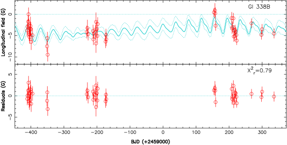
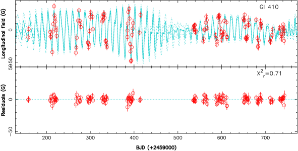
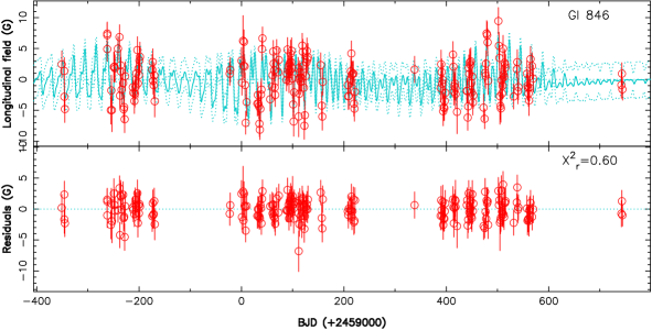
Figure 4: Same as Fig. 1 for Gl 338B (top), Gl 410 (middle) and Gl 846 (bottom).

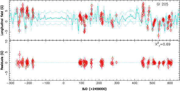
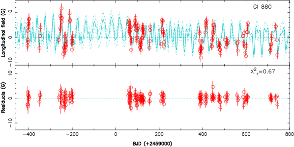
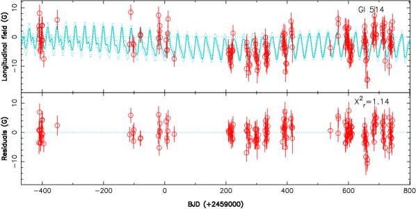
Figure 5: Same as Fig. 1 for Gl 205 (top), Gl 880 (middle) and Gl 514 (bottom).

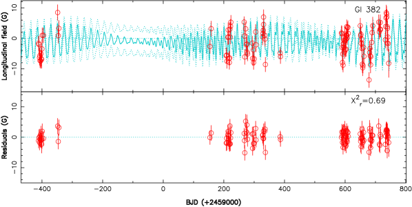
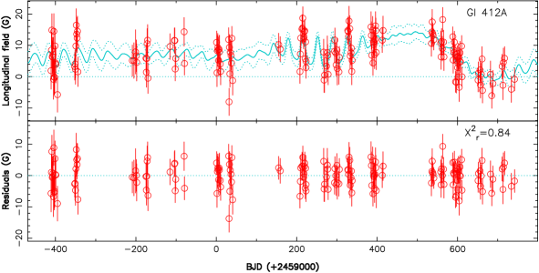
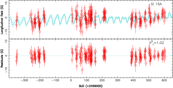
Figure 6: Same as Fig. 1 for Gl 382 (top), Gl 412A (middle) and Gl 15A (bottom).

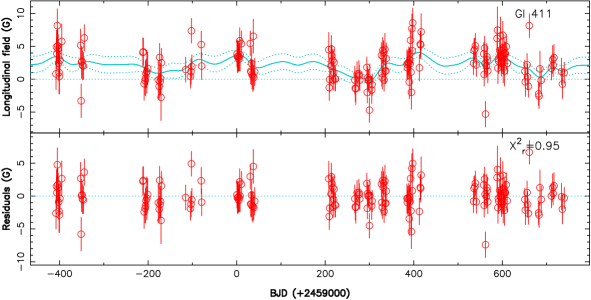
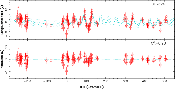
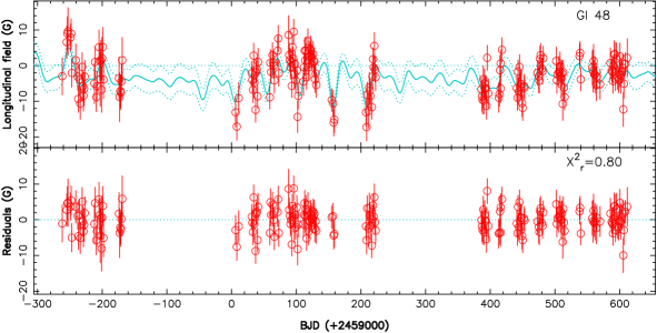
Figure 7: Same as Fig. 1 for Gl 411 (top), Gl 752A (middle) and Gl 48 (bottom).

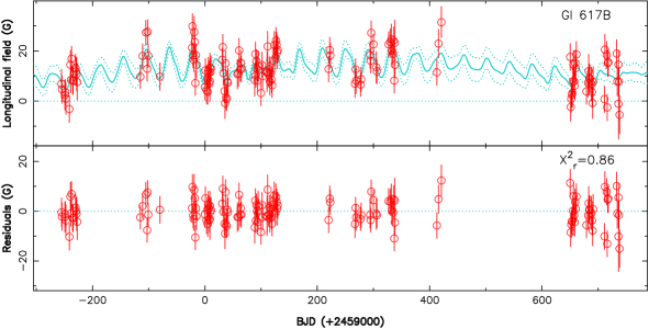
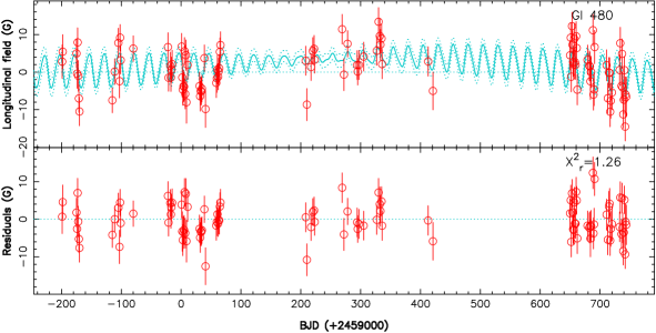
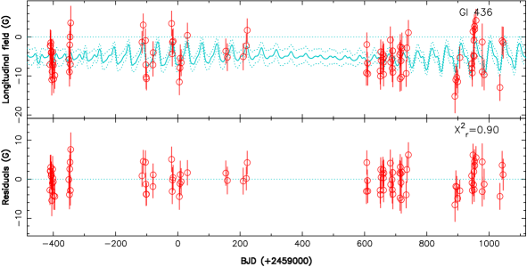
Figure 8: Same as Fig. 1 for Gl 617B (top), Gl 480 (middle) and Gl 436 (bottom).

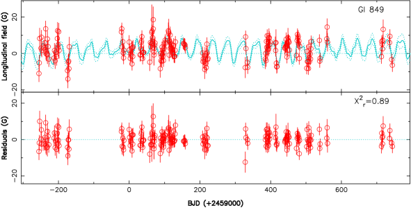
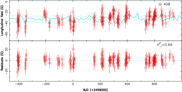
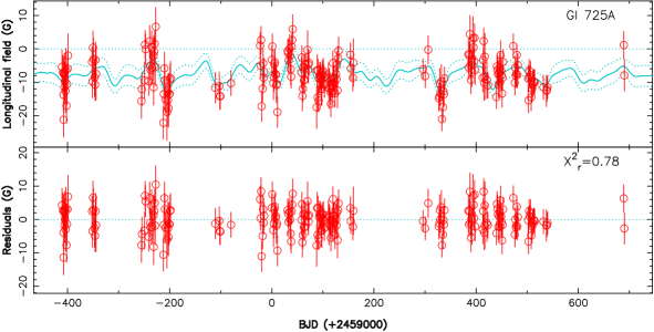
Figure 9: Same as Fig. 1 for Gl 849 (top), Gl 408 (middle) and Gl 725A (bottom).

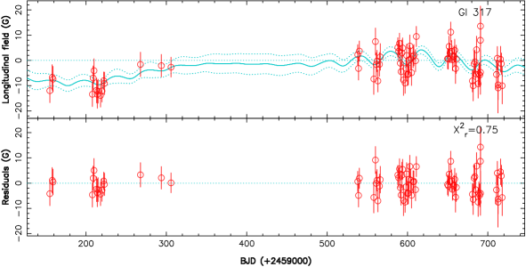
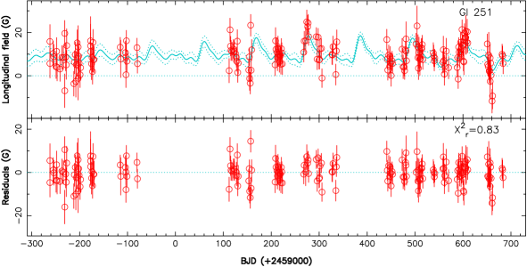
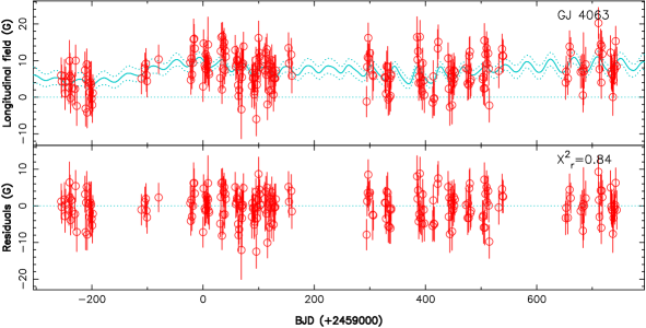
Figure 10: Same as Fig. 1 for Gl 317 (top), Gl 251 (middle) and GJ 4063 (bottom).

Table 3 summarizes the results obtained for the 43 stars of our sample. We obtain definite detections of the QP $B_{\rm\ell}$ fluctuations for 29 stars, and marginal detections for 9. Altogether, this is 11 more stars with either definite or marginal detections of the rotation period than in Fouqué et al. (2023), as a likely result of the different data reduction and analysis. Note that even in the case of definite detections, there is still a small chance that the derived period is off, e.g., when GPR confused the true period with an harmonic or an alias. For instance, the period we derive for Gl 846 is twice larger than that quoted in Fouqué et al. (2023); in this case, we made sure that $\Delta\log\mathcal{L}_{M}$ is significantly larger for our period than for that of Fouqué et al. (2023). For all other stars for which both studies derived rotation periods, estimates are consistent within error bars (see Sec. 6). GPR plots for all stars with definite or marginal detections of the QP $B_{\rm\ell}$ fluctuations (other than those of Fig. 1) plus Gl 436 (see Sec. 5) are shown in Figs. 4-15.

We stress that detecting the rotation period critically depends on whether $B_{\rm\ell}$ fluctuations are large enough, and therefore on the epochs at which stars are observed as these fluctuations significantly evolve with time. GJ 1151 is one obvious example (see Fig. 15 top panel), with the modulation barely visible for the first 2 seasons and getting much larger in 2022. We speculate that this is likely why no periodic modulation is detected yet for a few of our sample stars, including Gl 436 whose rotation period is already known (Bourrier et al., 2018). More spectropolarimetric observations of these targets are thus expected to end up revealing a clear periodicity at some point.

We note that the derived $\chi^{2}_{\rm r}$ of the GPR fit is on average smaller than 1 (<$\chi^{2}_{\rm r}$>$=0.86\pm 0.13$) and that $\theta_{5}$ is in most cases consistent with 0, confirming that our error bars are indeed slightly overestimated (by about 8% on average), as anticipated in Sec. 3. This is presumably why we sometimes obtain marginal (or even clear) detections of the $B_{\rm\ell}$ modulation for stars in which the field or its variation was listed as not formally detected in Table 2, like PM J21463+3813 and GJ 1002 (see Figs. 13 middle panel and 15 bottom panel).

We finally point out that the derived rotation periods, when coupled to the stellar radii listed in Table 1, yield equatorial rotation velocities lower than 2 km s^-1 for all stars, with a median value of 0.2 km s^-1, implying in practice undetectable rotational broadening of line profiles in SPIRou spectra.

5 Comments on individual stars

In this section, we discuss various specific points for about half the stars in our sample, focussing in particular on those for which clarifications are helpful. We do not discuss much the stars for which the periodicity of $B_{\rm\ell}$ data is detected very clearly (e.g., GJ 1289, Gl 880, Gl 905, Gl 205, Gl 410), apart from mentioning that the $B_{\rm\ell}$ curves we derive for GJ 1289, Gl 205 and Gl 410 (featuring peak-to-peak amplitudes in the range 150–200 G, 5–15 G and 40–90 G respectively) are consistent with those reported in previous studies based on optical ESPaDOnS and NARVAL data (Moutou et al., 2017; Hébrard et al., 2016; Donati et al., 2008). We do not discuss either the 3 stars (GJ 1012, Gl 445 and GJ 1105) where neither $B_{\rm\ell}$ nor its temporal variations and periodicity are detected.

5.1 Gl 338B

Gl 338B is one of the stars for which we have the fewest data points (50), hence why we fixed $\theta_{3}=120$ d, which is already on the long side for an early-M star. It is also one of the stars for which Fouqué et al. (2023) obtain no period from their $B_{\rm\ell}$ analysis. Our estimate ($42.2\pm 4.1$ d, see Fig. 4 top panel) is marginally reliable, featuring $\Delta\log\mathcal{L}_{M}=7.2$ with respect to the GPR fit including long-term modulation only. One other local maximum at $110\pm 17$ d shows up in the corner plot when we broaden the prior on $\theta_{2}$, with a slightly higher $\log\mathcal{L}_{M}$ (+1.8) than that of the main one we identified (at $42.2\pm 4.1$ d). Since the latter better matches the peak of the Lomb-Scargle periodogram (Press et al., 1992) of the $B_{\rm\ell}$ curve (located at 44 d), we kept it as the most likely despite the slightly smaller $\log\mathcal{L}_{M}$. We also note local maxima at 18 and 25 d (the first one close to the tentative period reported from activity indices by Sabotta et al., 2021), but with $\log\mathcal{L}_{M}$ values that are significantly lower than the 2 mentioned previously.

5.2 Gl 846

Gl 846 is one star for which the period we derive is different from (and twice larger than) that found by previous spectropolarimetric studies (Hébrard et al., 2016; Fouqué et al., 2023). There is indeed a local maximum near 11 d in the MCMC corner plot, which also corresponds to the main periodogram peak (at 11d); however, this local maximum period is much less probable than the main one we derive, with a likelihood contrast between the two of $\Delta\log\mathcal{L}_{M}=-27.3$. We thus confirm that the rotation period of Gl 846 is $21.84\pm 0.14$ d, which makes sense given the shape of the recorded $B_{\rm\ell}$ curve, showing only weak power in the first harmonics at some epochs (e.g., around BJD 2458800, see Fig. 4 bottom panel). The peak-to-peak amplitude of the $B_{\rm\ell}$ modulation that we derive, ranging from 10 to 20 G, is fully consistent with that found by Hébrard et al. (2016) from optical data.

5.3 Gl 412A

Gl 412A was listed in Fouqué et al. (2023) as exhibiting no periodic variations of $B_{\rm\ell}$ whereas we find a clear QP behaviour with a period of $36.9\pm 2.5$ d, significantly larger than where the main periodogram peak is located (28 d) in the period range 10–200 d. It reflects that $B_{\rm\ell}$ and its fluctuations evolve rapidly with time (see Fig. 6 middle panel), with a timescale $\theta_{3}\simeq 80$ d. We note in particular that the large-scale field of Gl 412A underwent rather drastic variations in our last observing season (2022). We also note that the period we derive does not agree with the current literature estimate (i.e., $100.9\pm 0.3$ d, Suárez Mascareño et al., 2018), where our GPR analysis finds no local maximum.

5.4 Gl 411

We find that Gl 411 exhibits a $B_{\rm\ell}$ modulation with a period of $427\pm 34$ d (see Fig. 7 top panel), consistent with that derived by Fouqué et al. (2023) and with the main periodogram peak (at 478 d). It is the longest period found in our sample, with no other peak at shorter periods, including harmonics. Although the $B_{\rm\ell}$ modulation is classified as being only marginally detected (see Sec. 3), the periodicity we detect is apparently reliable, with a $\Delta\log\mathcal{L}_{M}=11.9$ with respect to the GPR fit including long-term modulation only. If this period is indeed the rotation period, it would imply that Gl 411 is an unusually slow rotator for a mid-M dwarf; if the rotation period is in fact shorter (e.g., the one suggested by Díaz et al., 2019, i.e., $56.15\pm 0.17$ d), it would mean that the large-scale field of Gl 411 is nearly axisymmetric and generates undetectable rotational modulation of $B_{\rm\ell}$, but exhibits long-term QP intensity fluctuations with time, possibly as part of a much longer activity cycle.

5.5 Gl 617B

Gl 617B is another of the sample stars for which Fouqué et al. (2023) finds no rotation period, and with no published value suggested in the literature. We find clear periodicity in our $B_{\rm\ell}$ data at a period of $40.4\pm 3.0$ d (see Fig. 8 top panel), which coincides with the main peak of the periodogram (at 41 d). We note that the periodogram also shows significant power at about twice this period; besides, the GPR fit finds a local maximum at $86\pm 14$ d that is almost as likely as the main one ($\Delta\log\mathcal{L}_{M}=-1.5$) and could well be the true rotation period. The shorter period being more in line with those of our other samples stars of similar spectral type (except Gl 411, see above), we select it as the main one.

5.6 Gl 480

Like Gl 617B, Gl 480 has no published estimate of its rotation period, and Fouqué et al. (2023) did not succeed in deriving one. We find a fairly precise estimate of $25.00\pm 0.36$ d (see Fig. 8 middle panel), detected at almost the $\Delta\log\mathcal{L}_{M}=10$ threshold, and that exactly coincides with the maximum peak of the $B_{\rm\ell}$ periodogram. We note that another local maximum is identified by GPR at a much longer period (of $170\pm 14$ d), but whose significance is lower than the main one ($\Delta\log\mathcal{L}_{M}=-3.0$). We also find a third local maximum at about twice the rotation period we determined (i.e., $50.9\pm 1.3$ d and consistent with the period of the activity signal reported by Feng et al., 2020), but again with a significance that is even lower than the previous one ($\Delta\log\mathcal{L}_{M}=-4.0$).

5.7 Gl 436

This is again a star for which Fouqué et al. (2023) finds no period, and whose $B_{\rm\ell}$ is no more than marginally fluctuating at the time of our observations (see Sec. 3). There is however a fairly accurate period quoted in the literature ($44.09\pm 0.08$ d, Bourrier et al., 2018). Like in Fouqué et al. (2023), our GPR analysis concludes that the periodicity is not detected in our SPIRou data, even marginally. The period we derive, $48\pm 13$ d, is nonetheless consistent with the literature value (albeit with a much larger error bar), hence why we mention it in Table 3. We suspect that our non detection reflects that the $B_{\rm\ell}$ modulation was weak at the time of our observations (see Fig. 8 bottom panel), leading to no more than an insignificant difference in $\log\mathcal{L}_{M}$ between the GPR fits.

5.8 Gl 408

Gl 408 is another star for which our GPR analysis indicates clear periodicity of the $B_{\rm\ell}$ fluctuations (see Fig. 9 middle panel), and for which no literature estimate (including Fouqué et al., 2023) exists. The period we derive, equal to $171.0\pm 8.4$ d, is reliable (with a $\Delta\log\mathcal{L}_{M}$ contrast of 16.5 with respect to the GPR fit to long-term $B_{\rm\ell}$ variations only) and coincides well with the main periodogram peak (169 d). We fixed $\theta_{3}$ to a typical value of 200 d to help GPR converge given the small amplitude of the $B_{\rm\ell}$ variations.

5.9 Gl 317

Gl 317 is in a situation similar to Gl 480, with no known rotation period and none derived by Fouqué et al. (2023). We detect periodicity at a marginal level, with a period of $39.0\pm 3.8$ d, i.e., 3$\sigma$ lower than that given by the main peak of the periodogram (51 d) in the period range 10–200 d. The low number of data points (77) and moderate sampling both contribute at keeping this detection marginal (see Fig. 10 top panel).

5.10 GJ 4063

This is one of the few stars that features a $B_{\rm\ell}$ curve with low amplitude fluctuations, listed as non detected in Sec. 3. The GPR analysis nonetheless marginally detects periodicity in the data (at a level of $\Delta\log\mathcal{L}_{M}=7.9$, see Fig. 10 bottom panel) with a period of $40.7\pm 3.5$ d that coincides both with the main periodogram peak (at 40 d) in the 10-100 d range, and is consistent with the literature estimate (Díez Alonso et al., 2019). This gives us confidence that the period we find is likely the true one, despite being only marginally detected.

5.11 Gl 725B

With Gl 617B and Gl 408, Gl 725B is among the stars where we detect clear QP $B_{\rm\ell}$ variations (see Fig. 11 top panel), and for which no estimate of the rotation period is available in the literature (including Fouqué et al., 2023). The GPR analysis yields a period of $135\pm 15$ d, consistent within 1.3$\sigma$ with the main periodogram peak at 115 d, and features $\Delta\log\mathcal{L}_{M}$=12.9, i.e., a high enough contrast for the detection to be diagnosed as reliable.

5.12 PM J09553-2715

Like GJ 4063, PM J09553-2715 features low-amplitude $B_{\rm\ell}$ fluctuations in addition to limited sampling (see Fig. 11 middle panel), but the GPR analysis is able to retrieve a period ($73.0\pm 3.5$ d, consistent with that of Fouqué et al., 2023), with a marginal confidence level ($\Delta\log\mathcal{L}_{M}=6.8$).

5.13 GJ 1148

GJ 1148 is another star where $B_{\rm\ell}$ is detected, but not its variations according to our statistical test (Sec. 3). GPR is not able either to identify periodicity, even marginally, in the $B_{\rm\ell}$ data. A tentative periodicity shows up at $415\pm 54$ d, i.e., almost as long as that found for Gl 411, but only at a very low confidence level ($\Delta\log\mathcal{L}_{M}=1.8$). We note that Fouqué et al. (2023) find a similar long-period signal in their $B_{\rm\ell}$ data, although not reported explicitly in their paper.

5.14 PM J08402+3127

PM J08402+3127 features obvious long-term $B_{\rm\ell}$ variations, including a clear sign switch between our first and second observing season (see Fig. 12 middle panel). The $B_{\rm\ell}$ shorter-term modulation is weaker but nonetheless marginally detected with our QP GPR analysis, yielding a rotation period of $89.5\pm 8.0$ d with a moderate confidence level ($\Delta\log\mathcal{L}_{M}=7.6$, more than 2$\sigma$ away from the main periodogram peak at 70 d. The existing literature value ($118\pm 14$ d Díez Alonso et al., 2019), is at best marginally consistent with our new estimate.

5.15 Gl 699

Gl 699 is the star for which we have the largest number of visits (247), with both $B_{\rm\ell}$ and its time fluctuations clearly detected. Yet, the $B_{\rm\ell}$ curve is complex and evolving rapidly with time (see Fig. 13 top panel). As a result, the GPR modeling struggles to unambiguously determine the periodicity in the $B_{\rm\ell}$ curve, and to converge to the known rotation period (of $\simeq$140 d, e.g., Toledo-Padrón et al., 2019; Fouqué et al., 2023). The main peak in the periodogram, located at 69 d, indicates that the $B_{\rm\ell}$ modulation is dominated by the first harmonic. Coupled to the uneven sampling, it leads GPR into reducing the evolution timescale $\theta_{3}$ to values much smaller than the rotation period, and lowering the smoothing parameter $\theta_{4}$ as well, making it hard to pinpoint periodicity. We therefore fixed $\theta_{3}$ and $\theta_{4}$ to typical values, 100 d and 0.4 respectively, to help GPR converge. The period we find, $136\pm 13$ d, is consistent with the literature value, although with a rather large error bar.

5.16 PM J21463+3813

Although both $B_{\rm\ell}$ and its fluctuations are listed as non detected per our statistical test (Sec. 3), the GPR analysis is nonetheless able to find a periodicity (see Fig. 13 bottom panel), with a confidence level high enough to claim a definite detection ($\Delta\log\mathcal{L}_{M}=14.2$). The period we find, equal to $93.9\pm 3.4$ d, is consistent with the main peak in the periodogram (88d). No rotation period is mentioned in the literature for this star, including Fouqué et al. (2023) whose analysis did not succeed in detecting it.

5.17 Gl 447

Despite the sparse and very unevenly sampled data set, GPR is able to identify a tentative period from the clearly detected $B_{\rm\ell}$ values and temporal fluctuations (see Fig. 14 middle panel), equal to $24.1\pm 3.7$ d and in agreement with the main peak in the periodogram (at 23 d). The detection is only marginal, with $\Delta\log\mathcal{L}_{M}=7.5$, and may in fact be an artifact of the poor sampling (although the window function shows no peak in the corresponding period range). We note that this period is much shorter than that reported by Suárez Mascareño et al. (2016), and in fact suspiciously short for an inactive late-M dwarf like Gl 447. No period was reported in Fouqué et al. (2023).

5.18 GJ 1151

GJ 1151 is a perfect demonstration of the critical need of long-term monitoring for detecting periodicities, and more generally the large-scale magnetic field and its temporal evolution. As shown in Fig. 14 (bottom panel), $B_{\rm\ell}$ was no more than marginally detected in the first 2 seasons, making it ambiguous to determine a rotation period. In 2022 however, $B_{\rm\ell}$ started to exhibit a much larger modulation, from which GPR is able to safely retrieve a rotation period of $175.6\pm 4.9$ d, with one of the highest confidence level of the whole sample (($\Delta\log\mathcal{L}_{M}=75.2$), and located not far from the main peak in the periodogram (160 d). We stress that this period is consistent with the one derived by Fouqué et al. (2023), but different from the other existing literature estimates (e.g., Irwin et al., 2011; Díez Alonso et al., 2019).

5.19 GJ 1103

GJ 1103 is another star on which the temporal fluctuations of $B_{\rm\ell}$ are listed as non detected in Table 2 (Sec. 3), and for which the GPR analysis is able to identify a period (see Fig. 15 top panel). In fact, given the relative sparseness of the data, 2 periods show up, one being the first harmonic of the second. We find that the longer one, $142.6\pm 9.6$ d is slightly more likely than the shorter one, but only by a small amount ($\Delta\log\mathcal{L}_{M}=0.6$), with the main peak in the periodogram (at 76 d) coinciding with the first harmonic. This period is only marginally detected ($\Delta\log\mathcal{L}_{M}=9.1$) and is consistent with that derived by Fouqué et al. (2023).

5.20 GJ 1002

As for PM J21463+3813, GJ 1002 is listed in Table 2 as being non detected for both $B_{\rm\ell}$ and its temporal fluctuations, whereas the GPR analysis succeeds in digging out a periodicity (see Fig. 1 bottom panel), though at a marginal level ($\Delta\log\mathcal{L}_{M}=7.2$). The period we find, $89.8\pm 2.8$ d supports that of Fouqué et al. (2023) but not the recently published one of Suárez Mascareño et al. (2023).

6 Summary and discussion

We scrutinized the complete set of SPIRou observations for the sample of 43 M dwarfs studied by Fouqué et al. (2023), but reducing and analyzing the data with Libre-ESpRIT (the nominal ESPaDOnS reduction package optimized for spectropolarimetry and adapted for SPIRou, Donati et al., 1997; Donati et al., 2020) and with LSD (with VALD-3 M0 and M3 masks using lines deeper than 10% of the continuum) to reliably diagnose (with $\chi^{2}$ tests) whether $B_{\rm\ell}$ and temporal fluctuations are detected, and if $B_{\rm\ell}$ QP fluctuations are observed (using GPR and MCMC in a Bayesian framework). Our reduction tools are different from those used in Fouqué et al. (2023), where data were processed with APERO (the nominal SPIRou reduction package optimized for RV precision, Cook et al., 2022) and analyzed with a different implementation of LSD.

We find that the $B_{\rm\ell}$ values and error bars derived with our reference reduction tools, consistent with those from previous studies based on optical ESPaDOnS and NARVAL data for stars observed in both domains (e.g., Gl 205, Gl 410, Gl 846, GJ 1289, Donati et al., 2008; Hébrard et al., 2016; Moutou et al., 2017), are on average 2$-$3$\times$ smaller than those obtained by Fouqué et al. (2023). This issue, likely attributable to the alternate LSD implementation used in Fouqué et al. (2023) and to a lesser extent in the way $B_{\rm\ell}$ values are derived from LSD profiles, is currently being investigated by the team, but should not affect their conclusions regarding rotation periods.

Altogether, we find that only 3 stars in the whole sample (GJ 1012, Gl 445 and GJ 1105) show no $B_{\rm\ell}$ detection at all. In the remaining set of 40 stars, one shows no $B_{\rm\ell}$ modulation (GJ 1148, exhibiting no more than a very marginal low-amplitude variation with a long period of over 400 d), another one (Gl 436) features a low-amplitude modulation at the expected period, a third one (Gl 447) is so poorly sampled that the derived period of its weak modulation is suspicious. For seven others, we are able to measure a period with marginal confidence that we tentatively identify as the stellar rotation period. This is the first such measurement in the case of Gl 480 and Gl 317, whereas the period we derive is different from the literature value for Gl 338B and PM J08402+3127, and consistent with the most recent estimate for GJ 4063, PM J09553-2715 and GJ 1002 (the latter two in agreement with Fouqué et al., 2023). Last but not least, we obtain definite detections of the periodic $B_{\rm\ell}$ variations for 30 stars of our sample, for the first time in the case of Gl 617B, Gl 408, Gl 725B and PM J21463+3813, contradicting the existing literature estimate for Gl 846 and Gl 412A, and in agreement with Fouqué et al. (2023) for the remaining 24 stars. Out of the 27 stars for which Fouqué et al. (2023) derived a rotation period, we find a consistent estimate for 26 of them, and disagree for only one (Gl 846) for which the period we infer is twice longer (i.e., the fundamental vs the first harmonic for Fouqué et al. 2023). The comparison between rotation periods from both papers is shown in Fig. 2.

On average, the periods we measure are shorter for early-M stars than for mid- to late-M stars. For an unbiased sample of M dwarfs, the known trend is the opposite, with late-M dwarfs rotating statistically faster and being more active than early-M ones (e.g., Delfosse et al., 1998; Browning et al., 2010; West et al., 2015; Newton et al., 2016). Our result actually reflects that the SLS mainly focussed on inactive dwarfs to minimize the activity jitter in their RV curves, and therefore ended up discarding from the sample most late-M dwarfs with rotation periods shorter than a few tens of days (Moutou et al., 2017). Activity, known to grow with decreasing Rossby number Ro (defined as the rotation period normalised by the convective turnover time $\tau$, with $\tau$ ranging from 30 to 150 d from early- to late-type M dwarfs, e.g., Wright et al., 2018), is indeed stronger for late-M dwarfs than for early-M dwarfs at a given rotation period. One exception to our biased trend is Gl 411 for which we derive an ultra long period of $427\pm 34$ d, the longest of our whole sample. If it is indeed the rotation period, it may indicate that the evolution of Gl 411 was different from the bulk of our sample. However, the abundance analysis of Cristofari et al. (2022) does not suggest that this is the case, with Gl 411 being apparently a rather standard member of the thick galactic disc (along with Gl 699) with low [M/H] and high [$\alpha$/Fe] (the abundance of $\alpha$ elements with respect to Fe). Another option is that the rotation period of Gl 411 is much shorter (e.g., the one suggested by Díaz et al., 2019, i.e., $56.15\pm 0.17$ d) and went undetected because of a perfectly axisymmetric large-scale field (generating no rotational modulation of $B_{\rm\ell}$) over the full timescale of our observations. Besides, we find that large-scale magnetic fields tend to evolve faster (i.e., lower $\theta_{3}$) for the higher-mass stars of our sample (in agreement with Fouqué et al., 2023), which may simply reflect that these higher-mass stars are on average more active than the other sample stars.

Figure 2: Comparison between rotation periods and error bars derived in this paper (on the horizontal axis) with those of Fouqué et al. (2023, on the vertical axis) for the 27 stars for which Fouqué et al. (2023) measured a period (the dotted line depicting equality). Except for Gl 846 where Fouqué et al. (2023) retrieves the first harmonic, both studies are consistent within better than 2$\sigma$.

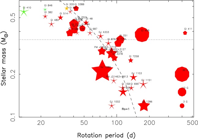
Figure 3: Properties of the large-scale field for the 38 stars of our sample for which a rotation period was measured, leaving out Gl 447 for which the recovered period is suspicious as a result of the sparse data set and poor sampling (see text). Symbol size depicts the strength of the large-scale field, whereas symbol shape describes the degree of axisymmetry (decagons for fully axisymmetric fields and stars for fully non-axisymmetric fields). Symbol color tentatively illustrates the field topology (red to blue for purely poloidal to purely toroidal fields) for the few stars in which the toroidal field is detected. The dashed line traces where Ro equals 1 (using convective turnover times from Wright et al., 2018), whereas the dotted line marks the mass below which M dwarfs become fully convective. The 3 red decagons in the bottom right corner indicate the symbol size for 3 typical values of the average longitudinal field.

Our results can be used to study how the large-scale magnetic fields of moderately- to weakly-active M dwarfs change with stellar parameters such as mass and rotation period, as in Donati & Landstreet (2009). To estimate in a simple way the average amount of magnetic energy in the large-scale field of each sample star, we quadratically sum the average $B_{\rm\ell}$ (second column of Table 2) and the semi-amplitude of the QP GP $\theta_{1}$ (third column of Table 3) fitted to the $B_{\rm\ell}$ curve, which can be respectively interpreted at first order as the amount of magnetic energy stored in the axisymmetric and non-axisymmetric components of the large-scale field. The latter two components can also be used to estimate the degree of axisymmetry of the large-scale field; for instance, a semi-amplitude $\theta_{1}$ much weaker than |<$B_{\rm\ell}$>| means a field that is mostly axisymmetric, whereas the opposite implies a field that is mostly non-axisymmetric.

Estimating the relative amount of magnetic energy in the poloidal and toroidal components (as in Donati & Landstreet, 2009) is more tricky, as the toroidal component is in fact hardly detectable in these low $v\sin i$ stars, except for the highest mass and fastest rotating targets of our sample (Lehmann & Donati, 2022) whose $v\sin i$ reaches up to $\simeq$1.5 km s^-1. By using Zeeman-Doppler Imaging (ZDI, Donati et al., 2006b) to carry out a preliminary analysis of our sample stars, we confirm that we are only able to detect a significant toroidal component (storing from 20 up to 50% of the magnetic energy) on 3 sample stars, namely Gl 410, Gl 846 and Gl 205, in agreement with previous studies based on optical (Donati et al., 2008; Hébrard et al., 2016; Moutou et al., 2017) and nIR (Cortés-Zuleta et al., 2023) data. For these 3 stars, we thus take the average amounts of toroidal energy derived with ZDI, whereas for all other stars, we assume that the field is fully poloidal. Note that it does not mean that the slowly rotating and / or less massive M dwarfs do not host significant toroidal fields, but rather that we are not able to detect them.

We show in Fig. 3 how our sample stars behave with respect to one another in a mass versus rotation period diagram, where the symbol size, shape and color illustrate the main characteristics of the large-scale field. As opposed to previous results on more massive and more rapidly rotating stars (Donati & Landstreet, 2009; Vidotto et al., 2014; See et al., 2015; Folsom et al., 2018) that all clearly demonstrate that their large-scale fields get weaker with increasing Ro, we do not see the same trend in our sample, with large-scale field being more or less constant in strength or even increasing with increasing Ro. We can see in particular stars rotating with periods of almost 200 d (like Gl 408, GJ 1151 or GJ 1286) hosting fields that are as strong or stronger than faster rotators (like GJ 1002, PM J21463+3813 or Gl 251). One trend that seems to emerge is that the lower mass dwarfs of our sample host fields that are less likely to be axisymmetric than the higher mass ones. All 14 stars with $\hbox{$M_{\star}$}<0.3$ ${\rm M}_{\odot}$ and whose longitudinal field is detected indeed exhibit mostly non-asisymmetric large-scale fields, whereas 9 of the remaining 24 higher mass dwarfs (10 out of 25 if we also include GJ 1148) feature mostly axisymmetric fields. Besides, we see no obvious sign that the bistable magnetic behaviour reported for rapidly rotating late-M dwarfs (Morin et al., 2010) also applies for the slowly-rotating ones. A more detailed study will require every single star of the sample to be studied with ZDI, the first of such papers concentrating on 6 of them (Gl 617B, Gl 408, GJ 1289, GJ 1151, Gl 905 and GJ 1286) being ready for publication (Lehmann et al., in prep). In parallel, a study of the small-scale fields of all sample stars will be carried out from the measurement of Zeeman broadening following Cristofari et al. (2023), which will allow us to diagnose how the large-scale and small-scale fields correlate with each other (Cristofari et al., in prep), as recently done for the young active M dwarf AU Mic (Donati et al., 2023).

Another interesting feature that our data reveal is that most slowly rotating M dwarfs, including fully convective ones, undergo obvious large-scale field variations, with some switching polarity during our monitoring like Gl 876 (Fig. 11 bottom panel, see also Moutou et al. 2023), PM J08402+3127 (Fig. 12 middle panel) and Gl 169.1A (Fig. 13 middle panel). Some other stars seem to succeed in amplifying their fields after a few years of relative magnetic quiescence like GJ 1151 (Fig. 14 bottom panel), or to achieve the opposite like Gl 905 (Fig. 15 middle panel). Ideally, one would like to pursue such monitoring on a timescale of at least a decade to investigate whether M dwarfs, and in particular fully-convective ones, undergo activity cycles as claimed by Route (2016) from radio observations, and to study how the properties of the large-scale fields evolve as stars progress along their cycle (Lehmann et al., 2021). This observational approach would give the opportunity of scrutinizing for the first time the physical processes at work in magnetic cycles of fully-convective stars that lack a tachocline, an ingredient whose role in generating solar-like magnetic cycles is still debated (Brun & Browning, 2017).

Spectropolarimetric observations with SPIRou at CFHT are already being pursued for some of our sample stars, both in the framework of the SPICE Large Programme (a follow-up of the SLS carried out from mid-2022 until mid-2024, and focussed mainly on the lowest mass dwarfs) and within a multi-semester PI program (PI: A. Carmona) targeting the most promising SLS targets in terms of planet detection and characterization. Altogether, additional observations will be collected for about 20 stars of our sample, that will be used to update our results in a couple of years and further confirm the rotation periods derived in Fouqué et al. (2023) and our paper.

Data availability

All data underlying this paper are part of the SLS, and will be publicly available from the Canadian Astronomy Data Center by February 2024.

Appendix A QP GPR fits to $B_{\rm\ell}$ data

In this appendix, we show the QP GPR fit to the $B_{\rm\ell}$ data for all stars of our sample exhibiting either clear or marginal periodicity (except those already shown in Fig. 1) plus that of Gl 436 (see main text in Sec. 5).

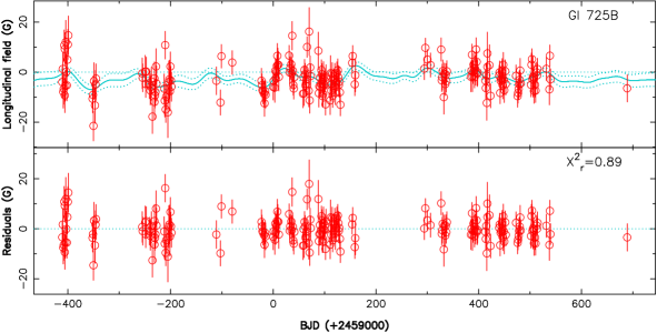
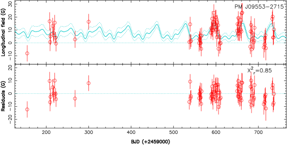
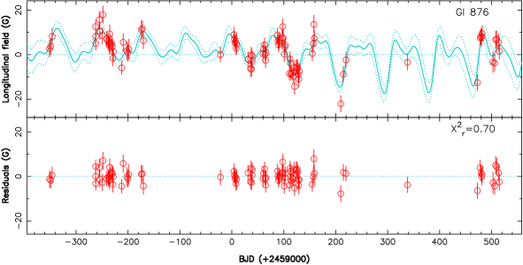
Figure 11: Same as Fig. 1 for Gl 725B (top), PM J09553-2715 (middle) and Gl 876 (bottom).

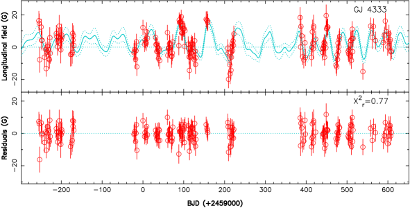
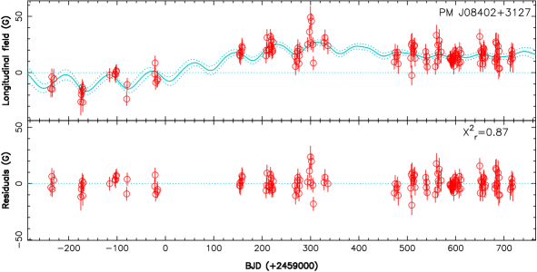
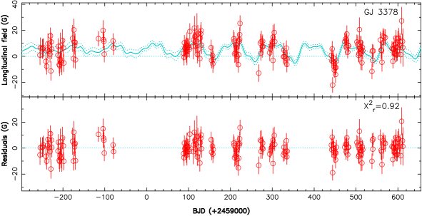
Figure 12: Same as Fig. 1 for GJ 4333 (top), PM J08402+3127 (middle) and GJ 3378 (bottom).

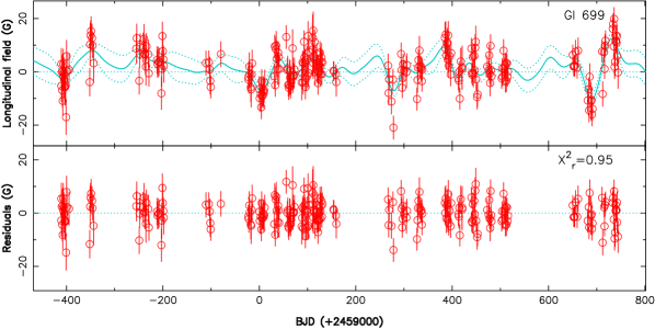
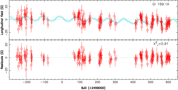
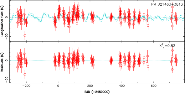
Figure 13: Same as Fig. 1 for Gl 699 (top), Gl 169.1A (middle), PM J21463+3813 (bottom).

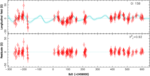
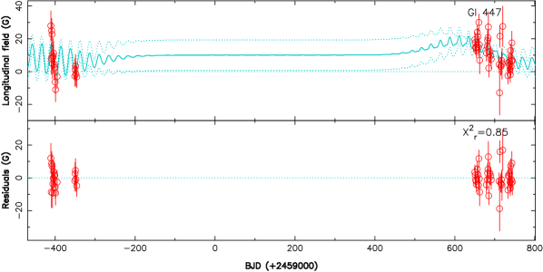
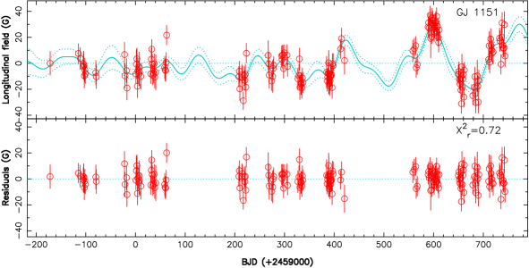
Figure 14: Same as Fig. 1 for Gl 15B (top), Gl 447 (middle) and GJ 1151 (bottom).

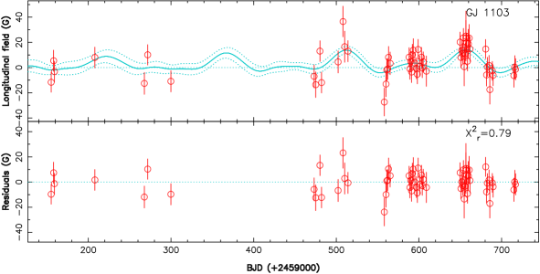
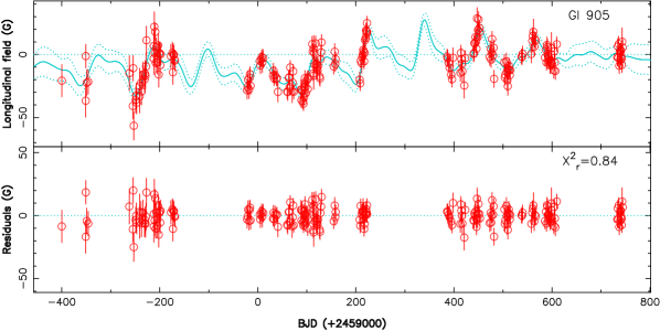
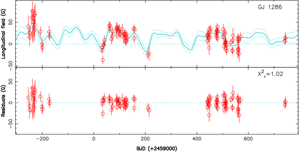
Figure 15: Same as Fig. 1 for GJ 1103 (top), Gl 905 (middle) and GJ 1286 (bottom).

References

- Babcock (1949) Babcock H. W., 1949, The Observatory, 69, 191
- Bonfils et al. (2013) Bonfils X., et al., 2013, A&A, 549, A109
- Bourrier et al. (2018) Bourrier V., et al., 2018, Nature, 553, 477
- Browning et al. (2010) Browning M. K., Basri G., Marcy G. W., West A. A., Zhang J., 2010, AJ, 139, 504
- Brun & Browning (2017) Brun A. S., Browning M. K., 2017, Living Reviews in Solar Physics, 14, 4
- Carmona et al. (2023) Carmona A., et al., 2023, A&A, 674, A110
- Cook et al. (2022) Cook N. J., et al., 2022, PASP, 134, 114509
- Cortés-Zuleta et al. (2023) Cortés-Zuleta P., et al., 2023, A&A, 673, A14
- Cristofari et al. (2022) Cristofari P. I., et al., 2022, MNRAS, 516, 3802
- Cristofari et al. (2023) Cristofari P. I., et al., 2023, MNRAS, 522, 1342
- Delfosse et al. (1998) Delfosse X., Forveille T., Perrier C., Mayor M., 1998, A&A, 331, 581
- Díaz et al. (2019) Díaz R. F., et al., 2019, A&A, 625, A17
- Díez Alonso et al. (2019) Díez Alonso E., et al., 2019, A&A, 621, A126
- Donati & Landstreet (2009) Donati J., Landstreet J. D., 2009, ARA&A, 47, 333
- Donati et al. (1997) Donati J.-F., Semel M., Carter B. D., Rees D. E., Collier Cameron A., 1997, MNRAS, 291, 658
- Donati et al. (2006a) Donati J.-F., Forveille T., Cameron A. C., Barnes J. R., Delfosse X., Jardine M. M., Valenti J. A., 2006a, Science, 311, 633
- Donati et al. (2006b) Donati J.-F., et al., 2006b, MNRAS, 370, 629
- Donati et al. (2008) Donati J.-F., et al., 2008, MNRAS, 390, 545
- Donati et al. (2020) Donati J. F., et al., 2020, MNRAS, 498, 5684
- Donati et al. (2023) Donati J. F., et al., 2023, MNRAS,
- Feng et al. (2020) Feng F., et al., 2020, ApJS, 250, 29
- Folsom et al. (2018) Folsom C. P., et al., 2018, MNRAS, 474, 4956
- Fouqué et al. (2023) Fouqué P., et al., 2023, A&A, 672, A52
- Gaidos et al. (2016) Gaidos E., Mann A. W., Kraus A. L., Ireland M., 2016, MNRAS, 457, 2877
- Hébrard et al. (2014) Hébrard É. M., Donati J.-F., Delfosse X., Morin J., Boisse I., Moutou C., Hébrard G., 2014, MNRAS, 443, 2599
- Hébrard et al. (2016) Hébrard É. M., Donati J. F., Delfosse X., Morin J., Moutou C., Boisse I., 2016, MNRAS, 461, 1465
- Irwin et al. (2011) Irwin J., Berta Z. K., Burke C. J., Charbonneau D., Nutzman P., West A. A., Falco E. E., 2011, ApJ, 727, 56
- Kiraga & Stepien (2007) Kiraga M., Stepien K., 2007, Acta Astronomica, 57, 149
- Kochukhov (2021) Kochukhov O., 2021, A&ARv, 29, 1
- Landstreet (1992) Landstreet J. D., 1992, A&ARv, 4, 35
- Lehmann & Donati (2022) Lehmann L. T., Donati J. F., 2022, MNRAS, 514, 2333
- Lehmann et al. (2021) Lehmann L. T., Hussain G. A. J., Vidotto A. A., Jardine M. M., Mackay D. H., 2021, MNRAS, 500, 1243
- Morin et al. (2008) Morin J., et al., 2008, MNRAS, 390, 567
- Morin et al. (2010) Morin J., Donati J., Petit P., Delfosse X., Forveille T., Jardine M. M., 2010, MNRAS, 407, 2269
- Moutou et al. (2017) Moutou C., et al., 2017, MNRAS, 472, 4563
- Moutou et al. (2023) Moutou C., et al., 2023, arXiv e-prints, p. arXiv:2307.11569
- Newton et al. (2016) Newton E. R., Irwin J., Charbonneau D., Berta-Thompson Z. K., Dittmann J. A., West A. A., 2016, ApJ, 821, 93
- Press et al. (1992) Press W. H., Teukolsky S. A., Vetterling W. T., Flannery B. P., 1992, Numerical recipes in C. The art of scientific computing
- Reiners (2012) Reiners A., 2012, Living Reviews in Solar Physics, 9, 1
- Reiners et al. (2010) Reiners A., Bean J. L., Huber K. F., Dreizler S., Seifahrt A., Czesla S., 2010, ApJ, 710, 432
- Reiners et al. (2022) Reiners A., et al., 2022, A&A, 662, A41
- Route (2016) Route M., 2016, ApJ, 830, L27
- Ryabchikova et al. (2015) Ryabchikova T., Piskunov N., Kurucz R. L., Stempels H. C., Heiter U., Pakhomov Y., Barklem P. S., 2015, Phys. Scr., 90, 054005
- Saar & Linsky (1985) Saar S. H., Linsky J. L., 1985, ApJ, 299, L47
- Sabotta et al. (2021) Sabotta S., et al., 2021, A&A, 653, A114
- See et al. (2015) See V., et al., 2015, MNRAS, 453, 4301
- Semel (1989) Semel M., 1989, A&A, 225, 456
- Shulyak et al. (2015) Shulyak D., Sokoloff D., Kitchatinov L., Moss D., 2015, MNRAS, 449, 3471
- Stibbs (1950) Stibbs D. W. N., 1950, MNRAS, 110, 395
- Strugarek et al. (2015) Strugarek A., Brun A. S., Matt S. P., Réville V., 2015, ApJ, 815, 111
- Suárez Mascareño et al. (2016) Suárez Mascareño A., Rebolo R., González Hernández J. I., 2016, A&A, 595, A12
- Suárez Mascareño et al. (2018) Suárez Mascareño A., et al., 2018, A&A, 612, A89
- Suárez Mascareño et al. (2023) Suárez Mascareño A., et al., 2023, A&A, 670, A5
- Toledo-Padrón et al. (2019) Toledo-Padrón B., et al., 2019, MNRAS, 488, 5145
- Vidotto et al. (2013) Vidotto A. A., Jardine M., Morin J., Donati J. F., Lang P., Russell A. J. B., 2013, A&A, 557, A67
- Vidotto et al. (2014) Vidotto A. A., et al., 2014, MNRAS, 441, 2361
- West et al. (2015) West A. A., Weisenburger K. L., Irwin J., Berta-Thompson Z. K., Charbonneau D., Dittmann J., Pineda J. S., 2015, ApJ, 812, 3
- Wright et al. (2018) Wright N. J., Newton E. R., Williams P. K. G., Drake J. J., Yadav R. K., 2018, MNRAS, 479, 2351