On the application of Gaussian graphical models to paired data problems

Abstract

Gaussian graphical models are nowadays commonly applied to the comparison of groups sharing the same variables, by jointy learning their independence structures. We consider the case where there are exactly two dependent groups and the association structure is represented by a family of coloured Gaussian graphical models suited to deal with paired data problems. To learn the two dependent graphs, together with their across-graph association structure, we implement a fused graphical lasso penalty. We carry out a comprehensive analysis of this approach, with special attention to the role played by some relevant submodel classes. In this way, we provide a broad set of tools for the application of Gaussian graphical models to paired data problems. These include results useful for the specification of penalty values in order to obtain a path of lasso solutions and an ADMM algorithm that solves the fused graphical lasso optimization problem. Finally, we present an application of our method to cancer genomics where it is of interest to compare cancer cells with a control sample from histologically normal tissues adjacent to the tumor. All the methods described in this article are implemented in the R package pdglasso availabe at https://github.com/savranciati/pdglasso.

Keywords: ADMM algorithm; Coloured Gaussian graphical model; Conditional independence; Fused lasso penalty; Graphical lasso; Symmetry.

1 Introduction

Graphical models are powerful tools for expressing the relationships between variables. In Gaussian graphical models (GGMs) the dependency structure is obtained by associating an undirected graph to the concentration matrix, that is the inverse of the covariance matrix. The graph has one vertex for every variable and every missing edge implies that the corresponding entry of the concentration matrix is equal to zero; see Lauritzen (1996).

In recent years, there has been a great deal of interest in the joint learning of multiple networks, where the observations come from two or more groups sharing the same variables. For instance, Danaher et al. (2014) considered the case of gene expression measurements collected from the cancer tissue of a sample of patients and from the normal tissue of a control sample. Hence, the association structure of each group is represented by a network and methods for the joint learning have been developed to deal with the fact that networks are expected to share similar patterns while retaining individual features. In this framework, the literature has mostly focused on the case where the groups are independent so that every network is a distinct unit, disconnected from the other networks; see Tsai et al. (2022) for a recent review. Thus, specific methods that deal with the across network association are required in the case where the groups are dependent. Xie et al. (2016) considered the case of gene expression data obtained from multiple tissues from the same individual and modelled the cross-graph dependence between groups by means of a latent vector representing systemic variation manifesting simultaneously in all groups; see also Zhang et al. (2022).

Roverato and Nguyen (2022, 2023) focused on paired data problems where there are exactly two dependent groups. Paired data are commonly originated from experimental designs where each subject is measured twice under two different conditions, or time points, as well as in matched pairs designs. For instance, in cancer genomics it is common practice to take control samples from histologically normal tissues adjacent to the tumor (Aran et al., 2017). Roverato and Nguyen (2022) approached the problem by considering a single GGM comprising the variables of both the first and the second group so that similarities between groups are represented by symmetries in the graph structure. One of the appealing features of this approach is that the resulting model has a graph for each of the two groups with the cross-graph dependence explicitly represented by the edges joining one group with the other, which may themselves present symmetries. Furthermore, in GGMs every entry of the concentration matrix can be naturally associated with either a vertex or an edge of the graph and thus every symmetry in the graph structure may possibly imply a parametric symmetry, in the sense of equalities in the associated concentration values. Hence, equality constraints encode stronger similarities and result in more parsimonious models.

GGMs with equality constraints in the parameter values were introduced in the seminal paper by Højsgaard and Lauritzen (2008), and are commonly known with the name of coloured GGMs because these constraints may be depicted on the dependence graph of the model by colouring of edges and vertices. Coloured GGMs with equality restrictions on the entries of the inverse covariance matrix form the family of RCON models (Højsgaard and Lauritzen, 2008), and here we focus on a subfamily of RCON models specifically suited for paired data problems, called RCON models for paired data (pdRCON models) by Roverato and Nguyen (2022).

Ranciati et al. (2021) considered the task of learning brain networks from fMRI data, and approached the problem by means of a fused graphical lasso procedure, named the symmetric graphical lasso, designed with the specific aim to identify symmetries between the left and the right hemisphere. In this paper, we introduce the graphical lasso for paired data (pdglasso) that extends the symmetric graphical lasso to deal with the wider family of pdRCON models. Hence, we carry out a comprehensive analysis of this approach, with special attention to the role played by relevant submodel classes implied by relationships between the two groups of specific interest in paired data problems.

One first case is when the covariance matrix has a two-block diagonal structure with blocks corresponds to the two groups, because in this case the two groups are independent and the corresponding subnetworks disconnected. Witten et al. (2011) provided the conditions for the solution to the graphical lasso to be block diagonal, and we show that this result holds true also for the pdglasso. Next, we consider the case where there are no differences between the two groups so that the resulting model is fully symmetric. Interestingly, fully symmetric pdRCON models form a subfamily of pdRCON models that is invariant under the permutation group naturally implied by the paired data problem (Højsgaard and Lauritzen, 2008; Gehrmann, 2011; Graczyk et al., 2022). Within this framework we provide a sufficient condition for the solution to the pdglasso to be a fully symmetric pdRCON model. A natural assumption when dealing with paired data is that pairs of homologous variables have equal partial variances, thereby leading to a submodel class with the property that the equality constraints in off-diagonal concentrations have a straightforward interpretation in terms of equality of partial correlation coefficients. Finally, parsimony can be achieved by focusing on submodel classes with fully symmetric structure either inside groups of across groups.

The results and methods presented in this paper are meant to provide an extensive set of tools for the immediate application of GGMs to the analysis of paired data. These also include an alternating directions method of multiplier (ADMM) algorithm that solves the pdglasso optimization problem and, furthermore, the R package (R Core Team, 2023) pdglasso that implements the ADMM algorithm as well as a function for the computation of maximum likelihood estimates and other utility functions to deal efficiently with the objects resulting from the analysis. For details about the package we refer to Section ‘Code and data availability’ of this paper. We then present an application of our methods to the analysis of gene expression data in cancer genomics.

The rest of this paper is organized as follows. Section 2 provides the background on coloured Gaussian graphical models and on graphical models for paired data, as required for this paper. The pdglasso problem is introduced in Section 3. Section 4 deals with fully symmetric models, and provides results useful for the specification of the amounts of penalization required to obtain a path of pdglasso solutions. Section 5 is devoted to some relevant families of submodels, whereas the application to gene expression data can be found in Section 6. Finally, Section 7 contains a brief discussion. Proofs are deferred to Appendices A and B, whereas Appendix C contains some illustrative examples of the models considered here. The ADMM algorithm for the optimization of the penalized likelihood can be found in Appendix D.

2 Coloured Gaussian graphical models for paired data

Let $Y_{V}$ be a continuous random vector indexed by a finite set $V=\{1,\ldots,p\}$. We denote by $\Sigma=\{\sigma_{ij}\}_{i,j\in V}$ and $\Sigma^{-1}=\Theta=\{\theta_{ij}\}_{i,j\in V}$ the covariance and the concentration matrix of $Y_{V}$, respectively. Both $\Sigma$ and $\Theta$ belong to the set $\mathcal{S}^{+}_{p}$ of (symmetric) $p\times p$ positive definite matrices and we assume, without loss of generality, that $E(Y_{V})=0$. An undirected graph with vertex set $V$ is a pair $\mathcal{G}=(V,E)$ where $E$ is an edge set that is a set of pairs of distinct vertices and, with a slight abuse of notation, we will write $\{i,j\}\in\mathcal{G}$, in place of $\{i,j\}\in E$, to mean that the edge $\{i,j\}$ belongs to $E$. We say that the concentration matrix $\Theta$ is adapted to a graph $\mathcal{G}=(V,E)$ if every missing edge of $\mathcal{G}$ corresponds to a zero entry if $\Theta$; formally, $\{i,j\}\not\in E$ implies $\theta_{ij}=0$ for every $i,j\in V$ with $i\neq j$. A Gaussian graphical model (GGM) with graph $\mathcal{G}$ is the family of multivariate normal distributions for $Y_{V}$ whose concentration matrix is adapted to $\mathcal{G}$. These models are also known with the name of covariance selection models or concentration graph models (Lauritzen, 1996).

In paired data problems, the set $V$ is naturally partitioned into a $L$eft and a $R$ight block, $V=L\cup R$ with $|L|=|R|=q=p/2$ and every variable in $Y_{L}$ has an homologous variable in $Y_{R}$. We set $i^{\prime}=i+q$ for every $i\in L$ and, without loss of generality, we index the variables so that $Y_{i}$ is homologous to $Y_{i^{\prime}}$ for every $i\in L$. In this way, it also holds that $L=\{1,\ldots,q\}$ and $R=\{q+1,\ldots,p\}$. Accordingly, the concentration matrix $\Theta$ can be naturally partitioned into four blocks,

$$\Theta=\left(\begin{array}[]{cc}\Theta_{LL}&\Theta_{LR}\\ \Theta_{RL}&\Theta_{RR}\\ \end{array}\right).$$ (3)

The subgraph of $\mathcal{G}$ induced by a subset $A\subseteq V$ is denoted by $\mathcal{G}_{A}=(A,E_{A})$, where $\{i,j\}\in E_{A}$ if and only if both $i,j\in A$ and $\{i,j\}\in E$. If $\Theta$ is adapted to $\mathcal{G}$ then it holds that $\Theta_{LL}$ and $\Theta_{RR}$ are adapted to $\mathcal{G}_{L}$ and $\mathcal{G}_{R}$, respectively. Thus, $\mathcal{G}_{L}$ and $\mathcal{G}_{R}$ are the group specific graphs and interest is for similarities involving the independence structures of the two groups, that we call structural symmetries. We distinguish between two types of structural symmetries. When for a pair $i,j\in L$, with $i\neq j$ the edges $\{i,j\}$ and $\{i^{\prime},j^{\prime}\}$ are either both present or both missing in $\mathcal{G}_{L}$ and $\mathcal{G}_{R}$, respectively, we say that there is an inside-block structural symmetry. On the other hand, $Y_{L}$ and $Y_{R}$ are not expected to be independent, and symmetries can also appear in the cross-group association structure, thereby involving the edges connecting the vertices in $L$ with the vertices in $R$. Hence, we say that an across-block structural symmetry is present if the edges $\{i,j^{\prime}\}$ and $\{i^{\prime},j\}$ are either both present or both missing in $\mathcal{G}$.

In a GGM, every diagonal entry of the concentration matrix can be associated with a vertex of $\mathcal{G}$, whereas every off-diagonal entry is associated with a pair of distinct vertices of the graph, and therefore to a possible edge. From this viewpoint, every structural symmetry due to a pair of missing edges also corresponds to a parametric symmetry because if, for example, both $\{i,j\}\not\in\mathcal{G}_{L}$ and $\{i^{\prime},j^{\prime}\}\not\in\mathcal{G}_{R}$, then also the associated parameters have the same value, $\theta_{ij}=\theta_{i^{\prime}j^{\prime}}=0$. This idea can be extended to symmetric pairs of non-missing edges, and we say that there is an inside-block parametric symmetry if for a pair $i,j\in L$, with $i\neq j$, it holds that $\theta_{ij}=\theta_{i^{\prime}j^{\prime}}$. On the other hand, across-block parametric symmetries are also possible in the case where, for some $i,j\in L$, it holds that $\theta_{ij^{\prime}}=\theta_{i^{\prime}j}$, with $i\neq j$. Finally, parametric symmetries can also be satisfied by the diagonal entries of $\Theta$ and we say that there is a vertex parametric symmetry if for $i\in L$ it holds that $\theta_{ii}=\theta_{i^{\prime}i^{\prime}}$. Appendix C gives some examples of pdRCON models with a detailed description of the different types of symmetries they may represent.

Gaussian graphical models with additional restrictions on the parameter space were introduced by Højsgaard and Lauritzen (2008) with the name of coloured GGMs. The family of coloured GGMs characterized by equality Restrictions on CONcentration values are known as RCON models, whereas the subfamily of RCON models comprising the equality constraints suited for paired data problems, as described above, was introduced by Roverato and Nguyen (2022) with the name of RCON models for paired data (pdRCON models); see also Ranciati et al. (2021) for an application of RCON models for paired data that only involves inside-block and vertex symmetries.

Coloured GGMs are typically represented by coloured graphs where vertices and edges depicted in black identify unconstrained parameters, whereas other colours are used to identify subsets of parameters which are constrained to having the same value. In this way, a different colour is required for every distinct equality constraint. We note, however, that this representation is redundant in the case of pdRCON models, because equality constraints may only involve specific pairs of parameters. Indeed, in order to identify the model from the graph it is sufficient to be able to distinguish whether a parameter is constrained or not. It follows that a pdRCON model can be unambiguously identified also if all the non-black vertices and edges are depicted of the same colour. This makes the graphical representation more readable for large graphs and, thus, here we will follow this rule and simply refer to coloured vertices and edges in contrast to uncoloured (i.e. black) ones.

3 The graphical lasso for paired data

For a sample $y^{(1)}_{V},\ldots,y^{(n)}_{V}$ of i.i.d. observations of $Y_{V}\sim N(0,\Sigma)$ the maximum likelihood estimator of $\Theta$ is the value that maximises the log-likelihood function

$$l(\Theta)=\log\det(\Theta)-\operatorname{tr}(S\Theta)$$ (4)

over $\mathcal{S}^{+}_{p}$ where $S=\{s_{ij}\}_{i,j\in V}$ is the matrix $S=n^{-1}\sum_{i=1}^{n}y^{(i)}_{V}(y^{(i)}_{V})^{\top}$. In GGMs the interest is for the zero pattern of $\Theta$ and Yuan and Lin (2007) proposed an estimator of $\Theta$ obtained from the minimization of the penalized log-likelihood

$$\mathcal{L}_{\lambda_{1}}(\Theta)=-l(\Theta)+\mathcal{P}_{\lambda_{1}}(\Theta)$$ (5)

with $\mathcal{P}_{\lambda_{1}}(\Theta)=\lambda_{1}\left\lVert\Theta\right\rVert_{1}$, where $\left\lVert\cdot\right\rVert_{1}$ denotes the $\ell_{1}$-norm, that is the sum of the absolute values of the entries of the matrix, and $\lambda_{1}$ is a nonnegative regularization parameter. The minimization of (5) over $\mathcal{S}^{+}_{p}$ is known as the graphical lasso problem and a number of algorithms have been proposed for its solution; see, among others, Friedman et al. (2008) and Boyd et al. (2011, Section 6.5). Unlike the maximum likelihood estimator, for $\lambda_{1}>0$ the solution to the graphical lasso exists also when $p>n$ so that $S$ will be singular. The high popularity of the graphical lasso is due to the fact that it performs simultaneously estimation and model selection within the family of GGMs. Indeed, due to the geometry of the $\ell_{1}$-penalty, some of the off-diagonal entries of concentration matrix are shrunk to exactly zero, with non-decreasing level of sparsity as $\lambda_{1}$ increases.

In order to perform simultaneously estimation and model selection within the family of pdRCON models we introduce an additional penalty term

$$\mathcal{Q}_{\lambda_{2}}(\Theta)=\lambda_{2}\left(\left\lVert\Theta_{LL}-\Theta_{RR}\right\rVert_{1}+\left\lVert\Theta_{LR}-\Theta_{RL}\right\rVert_{1}\right)$$ (6)

to (5) so as to obtain,

$$\mathcal{L}_{\lambda_{1},\lambda_{2}}(\Theta)=-l(\Theta)+\mathcal{P}_{\lambda_{1}}(\Theta)+\mathcal{Q}_{\lambda_{2}}(\Theta),$$ (7)

and estimate $\Theta$ by the paired data graphical lasso (pdglasso) estimator $\widehat{\Theta}=\operatorname*{arg\,min}_{\Theta}\mathcal{L}_{\lambda_{1},\lambda_{2}}(\Theta)$, where minimization is taken over $\mathcal{S}^{+}_{p}$.

Note that $\mathcal{Q}_{\lambda_{2}}(\Theta)$ in (6) is a fused type lasso penalty (Tibshirani et al., 2005; Hoefling, 2010) with regularization parameter $\lambda_{2}\geq 0$. For $\lambda_{2}=0$ the pdglasso estimator coincides with the graphical lasso estimator whereas positive values of $\lambda_{2}$ encourage parametric symmetries. More specifically, the term $\lambda_{2}\left\lVert\Theta_{LL}-\Theta_{RR}\right\rVert_{1}=\lambda_{2}\sum_{i\in L}|\theta_{ii}-\theta_{i^{\prime}i^{\prime}}|+\lambda_{2}\sum_{i,j\in L;i\neq j}|\theta_{ij}-\theta_{i^{\prime}j^{\prime}}|$ encourages both vertex parametric symmetries and inside-block parametric symmetries, whereas $\lambda_{2}\left\lVert\Theta_{LR}-\Theta_{RL}\right\rVert_{1}=\lambda_{2}\sum_{i,j\in L}|\theta_{ij^{\prime}}-\theta_{i^{\prime}j}|$ encourages across-block parametric symmetries; we remark that, in the latter sum, $|\theta_{ij^{\prime}}-\theta_{i^{\prime}j}|=0$ whenever $i=j$ because $\Theta$ is a symmetric matrix. Hence, like the graphical lasso, the pdglasso is a sparse estimate of $\Theta$ when $\lambda_{1}$ is large, and has many parametric symmetries when $\lambda_{2}$ is large.

The idea of using a fused penalty to induce equality constraints between concentration parameters is not new, and it was first introduced by Danaher et al. (2014) in the context of joint learning of multiple GGMs for independent samples. Subsequently, Ranciati et al. (2021) considered the case of two possibly non independent groups and the pdglasso problem in (7) extends the work of Ranciati et al. (2021) including also cross-group symmetries.

4 Solutions to the pdglasso

This section deals with some issues concerning the solutions to the pdglasso. We first describe the algorithm we have implemented for the optimization of (7) and, next, we provide some results which are helpful in the definition of a grid of $\lambda_{1}$ and $\lambda_{2}$ values so as to obtain a path of pdglasso solutions. Of special interest is the family of models resulting when the value of $\lambda_{2}$ is specified so as to achieve full symmetry.

4.1 Algorithm

Following Danaher et al. (2014) and Ranciati et al. (2021) we solve the problem (7) using an alternating directions method of multipliers (ADMM) algorithm that extends the algorithm given in Section 6.5 of Boyd et al. (2011) so as to include the fused penalty term in (6). This is obtained by splitting the procedure into two nested optimization problems both solved by a specific ADMM algorithm, and where the inner ADMM algorithm is written in a form that makes use of the results for the fused lasso signal approximator given in Friedman et al. (2007).

Our ADMM algorithm for the solution of the pdglasso in (7) is implemented in the function admm.pdglasso of the pdglasso package. This implementation extends the algorithm of Ranciati et al. (2021) to include across-block symmetries but, in fact, it has been designed to solve a problem somehow more general than (7), and it makes it possible for the user to optimize (7) either over the entire family of pdRCON models or over some given subfamilies of pdRCON models of specific interest, as detailed in Section 5 below. Furthermore, the function pdRCON.mle of the same package exploits the ADMM algorithm for the computation of the maximum likelihood estimate of a pdRCON model. We refer the reader to Appendix D for the technical details of our implementation of the algorithm.

4.2 Fully symmetric pdRCON models

One of the main motivations for the analysis of paired data is the need to identify similarities, i.e. symmetries, and differences between the two groups. Thus, in this framework, a central role is played by the subclass of pdRCON models that show no differences between the two groups. It is of theoretical interest to understand the properties of this model class and, furthermore, in applications it may be useful to estimate a model within this class because it could be regarded as a benchmark for the comparison with an arbitrarily selected model, and the quantification the amount of asymmetry it shows. We call these models fully symmetric because, as shown below, their parametric symmetries are not restricted to the equalities of concentration coefficients but extend to partial correlation coefficients, variances, covariances and correlation coefficients. Furthermore, we provide a result concerning the value of $\lambda_{2}$ such that the solution to the $pdglasso$ is fully symmetric model. An instance of fully symmetric pdRCON model is described in Example C.4 of Appendix C.

Formally, we say that a pdRCON model is fully symmetric if and only if both $\Theta_{LL}=\Theta_{RR}$ and $\Theta_{LR}=\Theta_{RL}$. It is worth recalling that the equality $\Theta_{LL}=\Theta_{RR}$ implies (i) full vertex parametric symmetry in the sense that $\theta_{ii}=\theta_{i^{\prime}i^{\prime}}$ for every $i\in L$ and (ii) both structural and parametric inside-block symmetry because $\theta_{ij}=\theta_{i^{\prime}j^{\prime}}$ for every $i,j\in L$ with $i\neq j$ also implies that $\theta_{ij}=0$ if and only if $\theta_{i^{\prime}j^{\prime}}=0$. Similarly, the equality $\Theta_{LR}=\Theta_{RL}$ implies both structural and parametric across-block symmetry.

As far as the interpretation of the model is of concern, a useful property of fully symmetric pdRCON models is that every inside and across-block parametric equality constraint, for instance $\theta_{ij}=\theta_{i^{\prime}j^{\prime}}$, also implies that the corresponding partial correlations have the same values, i.e. $\rho_{ij\mid V\setminus\{i,j\}}=\rho_{i^{\prime}j^{\prime}\mid V\setminus\{i^{\prime},j^{\prime}\}}$. This follows immediately from the fact that the partial correlation between $Y_{i}$ and $Y_{j}$ given the remaining variables can be computed from concentrations as $\rho_{ij\mid V\setminus\{i,j\}}=-\theta_{ij}/\sqrt{\theta_{ii}\theta_{jj}}$ (see, e.g. Lauritzen, 1996, Section 5.1.3) and in a fully symmetric model it also holds that both $\theta_{ii}=\theta_{i^{\prime}i^{\prime}}$ and $\theta_{jj}=\theta_{j^{\prime}j^{\prime}}$.

An equivalent way to define fully symmetric pdRCON models is by requiring that the random vector $(Y_{L},Y_{R})^{\top}$ has the same distribution as that of $(Y_{R},Y_{L})^{\top}$; that is $Y_{L}$ and $Y_{R}$ are exchangeable between them. This shows that fully symmetric pdRCON models belong the family of coloured GGMs which satisfy permutation symmetry, as defined in Højsgaard and Lauritzen (2008, Section 5); see also Gehrmann (2011) and Graczyk et al. (2022). More specifically, if we denote by $J$ be the permutation matrix that exchanges $Y_{L}$ and $Y_{R}$, i.e. $J\times(Y_{L},Y_{R})^{\top}=(Y_{R},Y_{L})^{\top}$, then we have,

$$J=\left(\begin{array}[]{cc}O_{q}&I_{q}\\ I_{q}&O_{q}\\ \end{array}\right)\quad\mbox{and thus}\quad J\Theta J=\left(\begin{array}[]{cc}\Theta_{RR}&\Theta_{RL}\\ \Theta_{LR}&\Theta_{LL}\\ \end{array}\right),$$

where $I_{q}$ and $O_{q}$ are the $q\times q$ identity and zero matrices, respectively. Recall that permutation matrices are orthogonal and, furthermore, $J$ is symmetric so that $J=J^{\top}=J^{-1}$. We can thus say that a pdRCON model is fully symmetric if and only if $J\Theta J=\Theta$, in words, if and only if $\Theta$ is invariant under the action of $J$. It is straightforward to see that the latter equality is equivalent to $(J\Theta J)^{-1}=\Theta^{-1}$ and thus to $J\Sigma J=\Sigma$, and this shows that in a fully symmetric model also $\Sigma$ is invariant under the action of $J$. This implies that parametric symmetry holds true also for to the entries of the variance matrix, that is $\Sigma_{LL}=\Sigma_{RR}$ and $\Sigma_{LR}=\Sigma_{RL}$ and it straightforward to see that also the correlation matrix $P$ satisfies the same property, i.e. both $P_{LL}=P_{RR}$ and $P_{LR}=P_{RL}$.

Finally, we notice that the results given in Højsgaard and Lauritzen (2008, Section 5.2) can be applied to show that, for this family of models, the maximum likelihood estimate of $\Theta$ can be obtained by applying to the matrix $\bar{S}=(S+JSJ)/2$ a standard algorithm for the corresponding GGM without symmetry restrictions, such as the iterative proportional scaling, or even explicitly if $\mathcal{G}$ is decomposable (Lauritzen, 1996, page 146).

The application of the pdglasso commonly requires the initial definition of a grid of values of $\lambda_{2}$ to identify a path of pdglasso solutions. To this aim it is useful to identify a value of $\lambda_{2}$ that returns a fully symmetric model, to be set as maximum value of the grid. This is given in the following.

Theorem 4.1.

A sufficient condition for the solution of the pdglasso to be invariant under the action of $J$, that is $\widehat{\Theta}=J\widehat{\Theta}J$, is that

$$\lambda_{2}\geq\max\left\{|s_{ij}-s_{i^{\prime}j^{\prime}}|/2,\;|s_{i^{\prime}j}-s_{ij^{\prime}}|/2;\;\;i,j\in L\right\}$$ (8)

Proof.

See Appendix A. ∎

4.3 Diagonal and block diagonal solutions

The pdglasso problem coincides with the graphical lasso in the case where $\lambda_{2}$ is set to zero, and it is a well-known result that if $\lambda_{1}\geq\max_{i,j\in V;i\neq j}|s_{ij}|$ then the solution to the graphical lasso is a diagonal matrix so that the selected graph is fully disconnected; see among others Mazumder and Hastie (2012, Section 2.1). This result is helpful, for instance, in the definition of a grid of $\lambda_{1}$ values to identify a path of graphical lasso solutions. It is shown in Proposition B.1 of Appendix B that this is still true in the pdglasso problem for any $\lambda_{2}\geq 0$.

In the application of the pdglasso it is also of interest the case where the solution $\widehat{\Theta}$ is block diagonal with $\widehat{\Theta}_{LR}=O_{q}$. Indeed, in this case there are no across-block edges and the two groups are independent. For the case where $\lambda_{2}=0$, i.e. in the graphical lasso, this problem was considered by Witten et al. (2011) and Mazumder and Hastie (2012) where it is shown that such block diagonal structure is obtained whenever $\lambda_{1}\geq\max_{i,j\in L}|s_{ij^{\prime}}|$, and in Proposition B.2 of Appendix B we show that this is still true in the pdglasso problem for any $\lambda_{2}\geq 0$.

5 pdRCON submodel classes

When fitting a pdRCON model to a set of data it may be useful to restrict the analysis to one of some relevant submodel classes. This may be motivated by a number of different reasons, including the interpretability of the selected model or the need to keep the model dimension low, for example when $n$ is small relative to $p$. Furthermore, the relevant research question may imply the restriction to a submodel class, as shown in Section 4.2 where fully symmetric models are implied by the assumption that there are no differences between groups.

The function admm.pdglasso of the pdglasso package implements a more flexible version of the fused penalty (6), given by

$$\mathcal{Q}_{\lambda_{2}}(\Theta)=\lambda_{2}^{(V)}\left\lVert\operatorname{diag}(\Theta_{LL})-\operatorname{diag}(\Theta_{RR})\right\rVert_{1}+\lambda_{2}^{(I)}\left\lVert\Theta_{LL}^{\ast}-\Theta_{RR}^{\ast}\right\rVert_{1}+\lambda_{2}^{(A)}\left\lVert\Theta_{LR}-\Theta_{RL}\right\rVert_{1}$$ (9)

where $\Theta_{LL}^{\ast}=\Theta_{LL}-\operatorname{diag}(\Theta_{LL})$ and, similarly for $\Theta_{RR}^{\ast}$; note that $\operatorname{diag}(\Theta)$ refers to a diagonal matrix having the same diagonal as $\Theta$. In this way, there is one regularization parameter associated with every type of parametric symmetry and, more specifically, $\lambda_{2}^{(V)}$ is associated with vertex symmetry, $\lambda_{2}^{(I)}$ with inside-block symmetry and $\lambda_{2}^{(A)}$ with across-block symmetry. For a given value of $\lambda_{2}>0$, each of the three $\lambda_{2}^{(\cdot)}$ parameters can take any of the values in the set $\{0,\lambda_{2},\texttt{Inf}\}$. For instance, the user can impose (i) no constraints involving vertex symmetries by setting $\lambda_{2}^{(V)}=0$, (ii) the amount of vertex symmetry regularisation implied by $\lambda^{(V)}_{2}=\lambda_{2}$ and (iii) full vertex symmetry by setting $\lambda_{2}^{(V)}=\texttt{Inf}$. The same can be done independently for $\lambda_{2}^{(I)}$ and $\lambda_{2}^{(A)}$ thereby allowing the user to select a model within one of $|\{0,\lambda_{2},\texttt{Inf}\}|^{3}=9$ different pdRCON submodel classes, and in the following we look at some of these submodels in more detail.

The restriction used to define an RCON model are linear in the concentration matrix so that the log-likelihood function in concave (Højsgaard et al., 2007; Højsgaard and Lauritzen, 2008; Gehrmann, 2011) and, thus, the pdglasso in (7) is a convex optimization problem. It is therefore computationally convenient to define symmetries in term of equality of concentration values. However, a drawback of this approach is that it is not straightforward to interpret the meaning of the equality of two nonzero off-diagonal concentrations. Højsgaard and Lauritzen (2008) also introduced the family of RCOR models, which are coloured GGMs defined by equalities between specified partial variances and partial correlations. In this case, the interpretation of the model constraints is straightforward but, on the other hand, RCOR  models are curved exponential families and the log-likelihood is not in general concave. Here, we notice that in the paired data setting it is commonly assumed that homologous variables have comparable variability and, more formally, it may be reasonable to assume the equality of partial variances, that is $\sigma^{2}_{ii\mid V\setminus\{i\}}=\sigma^{2}_{i^{\prime}i^{\prime}\mid V\setminus\{i^{\prime}\}}$ for every $i\in L$. This is equivalent to assuming that $\theta_{ii}=\theta_{i^{\prime}i^{\prime}}$ for every $i\in L$, because $\sigma^{2}_{ii\mid V\setminus\{i\}}=\theta_{ii}^{-1}$ (see, e.g. Lauritzen, 1996, Section 5.1.3) and, thus, that the analysis should be carried out within the subset of pdRCON models satisfying full vertex symmetry, obtained by setting $\lambda_{2}^{(V)}=\texttt{Inf}$. Interestingly, as explained in Section 4.2, in a pdRCON models with full vertex symmetry any equality constraint between two off-diagonal concentrations implies the equality of the corresponding partial correlations. In other words, the subfamily of pdRCON models with full vertex symmetry is also a subfamily of RCOR models and, thus, it is made up of models which are immediately interpretable.

It may be the case that the substantive research hypothesis underlying the analysis only concerns the comparison of the association structure of the first group with that of the second. More formally, the focus may be on the comparison of $\Theta_{LL}$ and $\Theta_{RR}$, which are adapted to $\mathcal{G}_{L}$ and $\mathcal{G}_{R}$, respectively, whereas the cross-group association $\Theta_{LR}$ is regarded as a nuisance parameter. In this case, across-block symmetries are of no interest and if the sample size is large it may make sense to set $\lambda_{2}^{(A)}=0$. On the other hand, for smaller sample sizes it is also possible to set $\lambda_{2}^{(A)}=\texttt{Inf}$ so as to impose full across-block symmetry with the aim to reduce model dimensionality.

Finally, we remark that it is possible to combine the three types of vertex, inside-block and across-block constraints in different ways according to the research hypothesis of interest and the need of parsimony in the selected model. For example, in the case where $\lambda_{2}^{(V)}=\lambda_{2}^{(I)}=\lambda_{2}^{(A)}=\texttt{Inf}$ one obtains the fully symmetric model of Section 4.2.

6 Analysis of breast cancer gene expression data

We illustrate the use of our proposed method in a gene expression paired data problem concerning breast cancer. The samples refer to $n=114$ individuals with both tumor and healthy adjacent tissue information, hence the paired data nature of the problem. A curated set of $q=89$ genes of the Hedgehog Pathway, known for their involvement in breast cancer (Song et al., 2014; Kubo et al., 2004), is extracted from MSigDB Collections (Subramanian et al., 2005). For each individual, we consider gene-level transcription estimates, that is $\text{log}_{2}(Y+1)$ transformed normalized counts, across the same set of selected genes in both tissues ($p=89\times 2=178$), which lead to the $114\times 178$ final data matrix for the analysis. The first $q$ columns refer to gene-level transcriptions for the tumor tissues, and the remaining from $q+1$ to $p$ for the healthy ones. In this section, we leverage a terminology closely related to the names of the functions implemented in the R package pdglasso, to facilitate the reader’s experience in reproducing the results shown in the following. For details about the package we refer to Section ‘Code and data availability’ of this paper.

We focus on two pdRCON submodel classes, identified by their set of restrictions on the values of $\lambda^{(V)}_{2}$, $\lambda^{(I)}_{2}$ and $\lambda^{(A)}_{2}$ in (9). The first model we consider (labelled as fV) is a pdRCON class where $\lambda^{(V)}_{2}=\texttt{Inf}$ and $\lambda^{(I)}_{2}=\lambda^{(A)}_{2}=\lambda_{2}$, so that we force parametric symmetries on the vertices and penalize with magnitude $\lambda_{2}$ the remaining blocks. This is motivated by the interpretability of the resulting model where every off-diagonal parametric symmetry coincides with the equality of the corresponding partial correlation coefficients, as explained in Section 5. The second model considered (labelled as fVIA) is a fully symmetric model, as described Section 4.2, which is obtained by setting $\lambda^{(V)}_{2}=\lambda^{(I)}_{2}=\lambda^{(A)}_{2}=\texttt{Inf}$. For both classes, conditional on an optimality criterion, we need to select the best value for $\lambda_{1}$ and within the class fV also the best $\lambda_{2}$. The optimality is defined based on the extended Bayesian Information Criterion (eBIC), which is (Foygel and Drton, 2010):

$$\text{eBIC}=-2l(\widehat{\Theta}^{\operatorname{mle}})+\log(n)\,d+4d\gamma\log(p),$$

with $\gamma=0.5$, as suggested by the literature, and using the maximum likelihood estimate of $\Theta$ as obtained with the function pdRCON.mle.

Thus, within each class, we fit 15 models with varying $\lambda_{1}$ and fixed $\lambda_{2}=0$, on an user-defined grid of potential values, and identify the optimal one as that achieving the lowest eBIC score. Conditional on the best $\lambda_{1}$, we perform a similar search on a grid of candidate values for $\lambda_{2}$. This sequential procedure is implemented through the function pdRCON.fit, where the user can specify the limits and denseness of the grids used in the optimal search, potentially leveraging the theoretical results we provided for $\lambda_{1}$ and $\lambda_{2},$ respectively, in Proposition B.1 of Appendix B and Theorem 4.1 of Section 4.2, which are computed by the function lams.max in our implementation. For the breast cancer data we are analyzing, the theoretical max values are respectively $\lambda_{1}^{\text{(max)}}=6.49$ and $\lambda_{2}^{\text{(max)}}=3.76$. The final models of the two classes, selected according to the eBIC, are respectively named mod${}_{\text{fV}}$ and mod${}_{\text{fVIA}}$. The resulting graphs, which are visually depicted in Figures E.1 and E.2 of Appendix E, are very sparse and, for this reason, in the following we will focus only on the symmetries, either structural and parametric, that involve edges which are present in the graphs. Accordingly, to ease the reading, we will simply talk of symmetries without recalling, all the times, that we are considering present edges.

Table 1: Summary statistics of graphs identified by with pdglasso: mod${}_{\text{fVIA}}$ (last column); mod${}_{\text{fV}}$ and its three submodels considered (second to fifth column); sub1${}_{\text{fV}}$: across-block edges set to zero; sub2${}_{\text{fV}}$: inside-block structural asymmetries removed; sub3${}_{\text{fV}}$: inside-block structural symmetries converted to parametric symmetries. All models have full vertex symmetry.

	Reference model and submodels
Summary	mod${}_{\text{fV}}$	sub1${}_{\text{fV}}$	sub2${}_{\text{fV}}$	sub3${}_{\text{fV}}$	fVIA
Total edges	133	125	52	133	391
Graph density	0.84 %	0.79 %	0. 33 %	0.84 %	2.48 %
inside block
Total edges	125	125	44	125	362
Structural (non-zero) symmetric edges	22	22	22	0	0
Parametric (non-zero) symmetric edges	22	22	22	44	362
across block
Total edges	8	0	8	8	29
Structural (non-zero) symmetric edges	0	0	0	0	0
Parametric (non-zero) symmetric edges	0	0	0	0	22

An overview of the structure of the models involved in this analysis is provided in Table 1. The graph associated to model mod${}_{\text{fV}}$ has an overall density lower than 1%, with inside-block density larger than the across-block one. In particular, the graph has only 8 edges connecting genes across the two different groups (tumor vs healthy), whereas the two inside-block subgraphs have (respectively) 68 edges connecting genes measured on tumor-affected tissues, and 57 edges between genes measured on the paired healthy tissues. The most connected gene inside each type of tissue is the one named LPR2. In the tumor samples, 19 out of the 68 edges ($28\%$) connect LPR2 to other inside-block genes and, among the 11 parametric symmetries of this block, 6 ($55\%$) refer to its (partial) correlation values. In the healthy samples, the inside-block dependence structure appears more organized around the connectedness of LPR2, with similar percentages of edges and symmetries involving this specific gene. Inspecting the across-block, 5 out of the total 8 edges ($63\%$) involve LPR2. It is worth noticing that although the fully parametric model mod${}_{\text{fVIA}}$ has an associated graph with a density almost three times that of mod${}_{\text{fV}}$, the number of parameters is only $1.3$ times that of the reference model, which means that parsimony is still achieved by considering all the parametric symmetries the model identifies (see last column of Table 1).

Table 2: Summary of Likelihood Ratio Tests (LRTs) performed on each submodel against the reference mod${}_{\text{fV}}$.

$H_{0}:$ submodel is preferable	mod${}_{\text{fV}}$	sub1${}_{\text{fV}}$	sub2${}_{\text{fV}}$	sub3${}_{\text{fV}}$
Number of parameters	211	203	130	200
Deviance	11914.14	11962.02	14108.64	12058.92
LRT value	-	47.88	2194.50	144.78
Degrees of freedom	-	8	81	11
Critical $\chi_{\alpha}$ quantile at $\alpha=0.05$	-	15.51	103.00	19.68

We also compare models mod${}_{\text{fV}}$ with three of its submodels: (i) sub1${}_{\text{fV}}$, where across-block edges are removed; (ii) sub2${}_{\text{fV}}$, where inside-block structural asymmetries are removed; (iii) sub3${}_{\text{fV}}$, where all inside-block structural symmetries are turned into parametric symmetries. The three submodels are not nested within one another but they all are with respect to mod${}_{\text{fV}}$. Each submodel is obtained by operating directly on the graph identified by the model mod${}_{\text{fV}}$, which in turn provides three new graphs to be used as inputs of the function pdRCON.mle to obtain the associated maximum likelihood estimates of the submodels.

We first consider model sub1${}_{\text{fV}}$. Unlike the case of independent samples, in paired data problems a key issue is represented by the cross-graph structure that encodes the across-group dependence. It is interesting to note that there are potentially $q^{2}=7921$ across-graph edges, but the selected model mod${}_{\text{fV}}$ shows a very sparse across-graph association structure with as few as 8 edges, most of which involving the gene LPR2. It is therefore of interest to quantify the significance of the across-graph structure by comparing the model mod${}_{\text{fV}}$ with its submodel sub1${}_{\text{fV}}$ obtained by assuming that the group specific subgraphs are disconnected, that is $\Theta_{LR}=O_{q}$. This comparison is carried out by means of the Likelihood Ratio Test (LRT) at a significance level of $\alpha=0.05$, given in Table 2, that shows that the observed value of the test statistic is too large compared to the critical value $\chi_{0.05;8}$ so that the model sub1${}_{\text{fV}}$ seems not to provide an adequate fit to the data, and thus we can conclude that the across-groups structure cannot be ignored, and should thus be retained.

In the comparison of the two groups, differences are represented by asymmetries, and this motivates the comparison of the selected model mod${}_{\text{fV}}$ with its submodels sub2${}_{\text{fV}}$ and sub3${}_{\text{fV}}$. As shown but juxtaposing the second and fourth column of Table 1, among the 125 inside-block edges of the reference model 81 are asymmetric edges and thus not involved in any structural or parametric symmetry and model sub2${}_{\text{fV}}$ is obtained by removing such 81 edges. Hence, comparing mod${}_{\text{fV}}$ with sub2${}_{\text{fV}}$ amounts to test the presence of structural differences between the group specific subgraphs. Finally, comparing mod${}_{\text{fV}}$ with sub3${}_{\text{fV}}$ amount to test if the model can be further simplified by assuming that every structural symmetry is also parametric. As shown in Table 2 the empirical evidence is in favor of the hypotheses that structural asymmetries are present and that not all structural symmetries are also parametric.

7 Conclusions

We have considered the problem of joint learning of GGMs for paired data, in an approach that implements a fused graphical lasso penalty to identify a model within a suited family of coloured graphical models. We have addressed a number of issues with the aim to provide the results and tools required for an immediate and knowledgeable application of the method. The latter include an ADMM algorithm for the optimization of the penalized likelihood, some results required when computing a path of lasso solutions, the description of the features of some model subfamilies of specific interest and, finally, an R package where all the methods have been implemented.

We deem that one appealing feature of our approach is the interpretation of the selected model. When the number of variables is large, it is not straightforward to visualize and interpret a GGMs, and this task is even more challenging when the analysis involves two or more, possibly dependent, networks. The application of pdRCON models is restricted to the case where two groups are considered, but it provides a transparent representation of the across group association. Furthermore, as shown in the application of Section 6, one can meaningfully summarize the relationship between groups by focusing on the amount of both structural and parametric symmetry/asymmetry. The scope of the analysis may also justify the restriction to specific submodels such as the model with full vertex symmetry of the fully symmetric model.

Code and data availability

For reproducibility reasons, both original data (downloaded from https://xenabrowser.net/) and sample covariance matrices are available as part of the R package pdglasso, together with their metadata information. All implemented scripts and functions used throughout the paper (and more) are available at the following GitHub repository: https://github.com/savranciati/pdglasso.

Funding

This work was supported by the Italian “Ministero dell’Università e della Ricerca” under Grant PRIN 2022SMNNKY.

Disclosure statement

The authors report there are no competing interests to declare.

Appendices

Appendix A Proof of Theorem 4.1

For a positive definite matrix $\Theta$ we set the matrix $\bar{\Theta}=\frac{1}{2}(\Theta+J\Theta J)$. Note that $J^{-1}=J$ so that $J\bar{\Theta}J=\frac{1}{2}(J\Theta J+JJ\Theta JJ)=\frac{1}{2}(J\Theta J+\Theta)=\bar{\Theta}$, that is, $\bar{\Theta}$ is invariant under the action of $J$. It is also worth remarking that $\bar{\Theta}$ is positive definite by construction.

We now show that if $\lambda_{2}$ is chosen to satisfy (8) then for any positive definite matrix $\Theta$ it holds that $\mathcal{L}_{\lambda_{1},\lambda_{2}}(\bar{\Theta})\leq\mathcal{L}_{\lambda_{1},\lambda_{2}}(\Theta)$ so that the matrix which minimises $\mathcal{L}_{\lambda_{1},\lambda_{2}}(\cdot)$ in (7) must be invariant under the action of $J$. Concretely, we show that $\mathcal{L}_{\lambda_{1},\lambda_{2}}(\bar{\Theta})-\mathcal{L}_{\lambda_{1},\lambda_{2}}(\Theta)\leq 0$ and, to this aim, we analyse, in turn, three components of this difference.

We first show that $\{-\log\det(\bar{\Theta})\}-\{-\log\det(\Theta)\}\leq 0$, which is equivalent to $\log\det(\Theta)\leq\log\det(\bar{\Theta})$ and therefore to $\det(\Theta)\leq\det(\bar{\Theta})$. Because both $\Theta$ and $J\Theta J$ are positive definite the following inequality holds (see, e.g., Lütkepohl, 1996, p. 55 eqn (14))

$$\det(\bar{\Theta})^{1/p} =\det\left(\frac{1}{2}\Theta+\frac{1}{2}J\Theta J\right)^{1/p}\geq\det\left(\frac{1}{2}\Theta\right)^{1/p}+\det\left(\frac{1}{2}J\Theta J\right)^{1/p}$$

$$=2\det\left(\frac{1}{2}\Theta\right)^{1/p}=\det(\Theta)^{1/p}$$

where we have used the facts that $\det(\Theta)=\det(J\Theta J)$, because $J$ is a permutation matrix, and that $\det\left(\frac{1}{2}\Theta\right)=\frac{1}{2^{p}}\det(\Theta)$. We have thus shown that $\det(\bar{\Theta})^{1/p}\geq\det(\Theta)^{1/p}$ and this immediately implies that $\det(\bar{\Theta})\geq\det(\Theta)$ as required.

We now show that $+\lambda_{1}\!\left\lVert\bar{\Theta}\right\rVert_{1}-\lambda_{1}\!\left\lVert\Theta\right\rVert_{1}\leq 0$, i.e, that $\left\lVert\bar{\Theta}\right\rVert_{1}-\left\lVert\Theta\right\rVert_{1}\leq 0$. We first notice that $\left\lVert\Theta\right\rVert_{1}$ can be computed on the block components (3) of $\Theta$ as follows,

$$\left\lVert\Theta\right\rVert_{1} =\left\lVert\Theta_{LL}\right\rVert_{1}+\left\lVert\Theta_{RR}\right\rVert_{1}+\left\lVert\Theta_{LR}\right\rVert_{1}+\left\lVert\Theta_{RL}\right\rVert_{1}.$$

Similarly,

$$\left\lVert\bar{\Theta}\right\rVert_{1} =\left\lVert\bar{\Theta}_{LL}\right\rVert_{1}+\left\lVert\bar{\Theta}_{RR}\right\rVert_{1}+\left\lVert\bar{\Theta}_{LR}\right\rVert_{1}+\left\lVert\bar{\Theta}_{RL}\right\rVert_{1}$$

$$=\frac{1}{2}(\left\lVert\Theta_{LL}+\Theta_{RR}\right\rVert_{1}+\left\lVert\Theta_{RR}+\Theta_{LL}\right\rVert_{1}+\left\lVert\Theta_{LR}+\Theta_{RL}\right\rVert_{1}+\left\lVert\Theta_{RL}+\Theta_{LR}\right\rVert_{1})$$

$$=\left\lVert\Theta_{LL}+\Theta_{RR}\right\rVert_{1}+\left\lVert\Theta_{LR}+\Theta_{RL}\right\rVert_{1}.$$

Hence,

$$\left\lVert\bar{\Theta}\right\rVert_{1}-\left\lVert\Theta\right\rVert_{1} =\left\lVert\Theta_{LL}+\Theta_{RR}\right\rVert_{1}-(\left\lVert\Theta_{LL}\right\rVert_{1}+\left\lVert\Theta_{RR}\right\rVert_{1})$$

$$+\left\lVert\Theta_{LR}+\Theta_{RL}\right\rVert_{1}-(\left\lVert\Theta_{LR}\right\rVert_{1}+\left\lVert\Theta_{RL}\right\rVert_{1}),$$

and it follows that $\left\lVert\bar{\Theta}\right\rVert_{1}-\left\lVert\Theta\right\rVert_{1}\leq 0$ because for any pair of real numbers $a$ and $b$ it holds that $|a+b|\leq|a|+|b|$.

In order to complete the proof we have now to show that

$$\operatorname{tr}(S\bar{\Theta})-\operatorname{tr}(S\Theta)-\lambda_{2}\left(\left\lVert\Theta_{LL}-\Theta_{RR}\right\rVert_{1}+\left\lVert\Theta_{LR}-\Theta_{RL}\right\rVert_{1}\right)\leq 0.$$ (A.1)

Note that the term $\lambda_{2}\left(\left\lVert\bar{\Theta}_{LL}-\bar{\Theta}_{RR}\right\rVert_{1}+\left\lVert\bar{\Theta}_{LR}-\bar{\Theta}_{RL}\right\rVert_{1}\right)$ does not appear in (A.1) because it is equal to zero by construction. We first consider the difference

$$\operatorname{tr}(S\bar{\Theta})-\operatorname{tr}(S\Theta) =\operatorname{tr}(S\bar{\Theta}-S\Theta)=\operatorname{tr}\{S(\bar{\Theta}-\Theta)\}=\operatorname{tr}\{S(\frac{1}{2}\Theta+\frac{1}{2}J\Theta J-\Theta)\}$$

$$=\operatorname{tr}\{\frac{1}{2}S(J\Theta J-\Theta)\}=\frac{1}{2}\sum_{i=1}^{p}\sum_{j=1}^{p}s_{ij}(J\Theta J-\Theta)_{ij},$$ (A.2)

where (A.2) follows from the fact that both $S$ and $(J\Theta J-\Theta)$ are symmetric matrices. Hence, if we write (A.2) by distinguishing the terms corresponding to each of the four blocks of $(J\Theta J-\Theta)$ as in (3) we obtain,

$$\operatorname{tr}(S\bar{\Theta})-\operatorname{tr}(S\Theta) =\frac{1}{2}\sum_{i=1}^{q}\sum_{j=1}^{q}\{s_{ij}(\theta_{i^{\prime}j^{\prime}}-\theta_{ij})+s_{i^{\prime}j^{\prime}}(\theta_{ij}-\theta_{i^{\prime}j^{\prime}})+s_{ij^{\prime}}(\theta_{i^{\prime}j}-\theta_{ij^{\prime}})+s_{i^{\prime}j}(\theta_{ij^{\prime}}-\theta_{i^{\prime}j})\}$$

$$=\frac{1}{2}\sum_{i=1}^{q}\sum_{j=1}^{q}\{(s_{i^{\prime}j^{\prime}}-s_{ij})(\theta_{ij}-\theta_{i^{\prime}j^{\prime}})+(s_{i^{\prime}j}-s_{ij^{\prime}})(\theta_{ij^{\prime}}-\theta_{i^{\prime}j})\}$$ (A.3)

$$\leq\frac{1}{2}\sum_{i=1}^{q}\sum_{j=1}^{q}(|s_{i^{\prime}j^{\prime}}-s_{ij}||\theta_{ij}-\theta_{i^{\prime}j^{\prime}}|+|s_{i^{\prime}j}-s_{ij^{\prime}}||\theta_{ij^{\prime}}-\theta_{i^{\prime}j}|).$$ (A.4)

Furthermore,

$$\lambda_{2}\left(\left\lVert\Theta_{LL}-\Theta_{RR}\right\rVert_{1}+\left\lVert\Theta_{LR}-\Theta_{RL}\right\rVert_{1}\right)=\sum_{i=1}^{q}\sum_{j=1}^{q}\lambda_{2}\left(|\theta_{ij}-\theta_{i^{\prime}j^{\prime}}|+|\theta_{ij^{\prime}}-\theta_{i^{\prime}j}|\right).$$ (A.5)

Hence, from (A.3), (A.5) and then (A.4) we obtain

$$=\operatorname{tr}(S\Theta)-\operatorname{tr}(S\Theta)-\lambda_{2}\left(\left\lVert\Theta_{LL}-\Theta_{RR}\right\rVert_{1}+\left\lVert\Theta_{LR}-\Theta_{RL}\right\rVert_{1}\right)$$

$$=\frac{1}{2}\sum_{i=1}^{q}\sum_{j=1}^{q}\{(s_{i^{\prime}j^{\prime}}-s_{ij})(\theta_{ij}-\theta_{i^{\prime}j^{\prime}})+(s_{i^{\prime}j}-s_{ij^{\prime}})(\theta_{ij^{\prime}}-\theta_{i^{\prime}j})-\sum_{i=1}^{q}\sum_{j=1}^{q}\lambda_{2}\left(|\theta_{ij}-\theta_{i^{\prime}j^{\prime}}|+|\theta_{ij^{\prime}}-\theta_{i^{\prime}j}|\right)$$

$$\leq\frac{1}{2}\sum_{i=1}^{q}\sum_{j=1}^{q}(|s_{i^{\prime}j^{\prime}}-s_{ij}||\theta_{ij}-\theta_{i^{\prime}j^{\prime}}|+|s_{i^{\prime}j}-s_{ij^{\prime}}||\theta_{ij^{\prime}}-\theta_{i^{\prime}j}|)-\sum_{i=1}^{q}\sum_{j=1}^{q}\lambda_{2}\left(|\theta_{ij}-\theta_{i^{\prime}j^{\prime}}|+|\theta_{ij^{\prime}}-\theta_{i^{\prime}j}|\right)$$

$$=\sum_{i=1}^{q}\sum_{j=1}^{q}\left\{\left(|s_{i^{\prime}j^{\prime}}-s_{ij}|/2-\lambda_{2}\right)|\theta_{ij}-\theta_{i^{\prime}j^{\prime}}|+\left(|s_{i^{\prime}j}-s_{ij^{\prime}}|/2-\lambda_{2}\right)|\theta_{ij^{\prime}}-\theta_{i^{\prime}j}|\right\},$$

that establishes (A.1) because we have assumed that $\lambda_{2}$ satisfies (8) so that both $(|s_{i^{\prime}j^{\prime}}-s_{ij}|/2-\lambda_{2})$ and $(|s_{i^{\prime}j}-s_{ij^{\prime}}|/2-\lambda_{2})$ are smaller or equal to zero for every $i,j\in L$.

Appendix B Results concerning the choice of $\lambda_{1}$

Here we provide a formal proof of the two results concerning the values of $\lambda_{1}$ stated in an informal way in Subsection 4.3.

Proposition B.1.

A sufficient condition for the solution $\widehat{\Theta}$ to the pdglasso to be a diagonal matrix is that $|s_{ij}|\leq\lambda_{1}$ for every $i,j\in V$ with $i\neq j$.

Proof.

For a positive definite matrix $\Theta$ we denote by $\bar{\Theta}$ the diagonal matrix with the same diagonal as $\Theta$, that is $\bar{\Theta}=\operatorname{diag}(\Theta)$, and note that $\bar{\Theta}$ is positive definite by construction. Hence, we now show that if $\lambda_{1}\geq|s_{ij}|$ for every $i\neq j\in V$ then for any positive definite matrix $\Theta$ it holds that $\mathcal{L}_{\lambda_{1},\lambda_{2}}(\bar{\Theta})\leq\mathcal{L}_{\lambda_{1},\lambda_{2}}(\Theta)$ so that the matrix which minimises $\mathcal{L}_{\lambda_{1},\lambda_{2}}(\cdot)$ in (7) must be diagonal. Concretely, we show that $\mathcal{L}_{\lambda_{1},\lambda_{2}}(\bar{\Theta})-\mathcal{L}_{\lambda_{1},\lambda_{2}}(\Theta)\leq 0$ and, to this aim, we analyse, in turn, three components of this difference.

We first show that $\{-\log\det(\bar{\Theta})\}-\{-\log\det(\Theta)\}\leq 0$. The latter is equivalent to $\log\det(\Theta)\leq\log\det(\bar{\Theta})$, and therefore to $\det(\Theta)\leq\det(\bar{\Theta})$, which follows immediately from Hadamard’s inequality; see, for instance, Lütkepohl (1996, p. 54 eqn (3)).

We now show that $\operatorname{tr}(S\bar{\Theta})-\operatorname{tr}(S\Theta)+\lambda_{1}\!\left\lVert\bar{\Theta}\right\rVert_{1}-\lambda_{1}\!\left\lVert\Theta\right\rVert_{1}\leq 0$. Firstly, we notice that

$$\operatorname{tr}(S\bar{\Theta})-\operatorname{tr}(S\Theta)=\operatorname{tr}(S\bar{\Theta}-S\Theta)=\operatorname{tr}\{S(\bar{\Theta}-\Theta)\}=-\sum_{i=1}^{p}\sum_{\underset{j\neq i}{j=1}}^{p}s_{ij}\theta_{ij}\leq\sum_{i=1}^{p}\sum_{\underset{j\neq i}{j=1}}^{p}|s_{ij}||\theta_{ij}|,$$

where the third equality follows form the fact that both $S$ and $(\bar{\Theta}-\Theta)$ are symmetric matrices and, more specifically, that $(\bar{\Theta}-\Theta)$ is the matrix obtained by setting to zero the diagonal entries of $-\Theta$. Similarly,

$$\lambda_{1}\!\left\lVert\bar{\Theta}\right\rVert_{1}-\lambda_{1}\!\left\lVert\Theta\right\rVert_{1}=-\sum_{i=1}^{p}\sum_{\underset{j\neq i}{j=1}}^{p}\lambda_{1}|\theta_{ij}|;$$

so that,

$$\operatorname{tr}(S\bar{\Theta})-\operatorname{tr}(S\Theta)+\lambda_{1}\!\left\lVert\bar{\Theta}\right\rVert_{1}-\lambda_{1}\!\left\lVert\Theta\right\rVert_{1} =-\sum_{i=1}^{p}\sum_{\underset{j\neq i}{j=1}}^{p}s_{ij}\theta_{ij}-\sum_{i=1}^{p}\sum_{\underset{j\neq i}{j=1}}^{p}\lambda_{1}|\theta_{ij}|$$

$$\leq\sum_{i=1}^{p}\sum_{\underset{j\neq i}{j=1}}^{p}|s_{ij}||\theta_{ij}|-\sum_{i=1}^{p}\sum_{\underset{j\neq i}{j=1}}^{p}\lambda_{1}|\theta_{ij}|$$

$$=\sum_{i=1}^{p}\sum_{\underset{j\neq i}{j=1}}^{p}(|s_{ij}|-\lambda_{1})|\theta_{ij}|\leq 0,$$

where the latter inequality holds true because, by assumption, $(|s_{ij}|-\lambda_{1})\leq 0$ for every $i\neq j\in V$.

Finally, we show that the difference

$$\lambda_{2}\left(\left\lVert\bar{\Theta}_{LL}-\bar{\Theta}_{RR}\right\rVert_{1}+\left\lVert\bar{\Theta}_{LR}-\bar{\Theta}_{RL}\right\rVert_{1}\right)-\lambda_{2}\left(\left\lVert\Theta_{LL}-\Theta_{RR}\right\rVert_{1}+\left\lVert\Theta_{LR}-\Theta_{RL}\right\rVert_{1}\right)$$ (B.1)

is smaller or equal to zero. We first note that $\left\lVert\bar{\Theta}_{LR}-\bar{\Theta}_{RL}\right\rVert_{1}=0$ because $\bar{\Theta}$ is diagonal and, next, that $\left\lVert\bar{\Theta}_{LL}-\bar{\Theta}_{RR}\right\rVert_{1}-\left\lVert\Theta_{LL}-\Theta_{RR}\right\rVert_{1}=-\sum_{i=1}^{p}\sum_{\underset{j\neq i}{j=1}}^{p}|\theta_{ij}-\theta_{i^{\prime}j^{\prime}}|$. Hence, (B.1) can be written as

$$-\sum_{i=1}^{q}\sum_{\underset{j\neq i}{j=1}}^{q}\lambda_{2}|\theta_{ij}-\theta_{i^{\prime}j^{\prime}}|-\sum_{i=1}^{q}\sum_{j=1}^{q}\lambda_{2}|\theta_{ij^{\prime}}-\theta_{i^{\prime}j}|$$

that is trivially non-positive because $\lambda_{2}\geq 0$, and this completes the proof. ∎

Proposition B.2.

A sufficient condition for the solution $\widehat{\Theta}$ to the pdglasso to be block diagonal with blocks $\widehat{\Theta}_{LL}$ and $\widehat{\Theta}_{RR}$ is that $|s_{ij}|\leq\lambda_{1}$ for every $i\in L$ and $j\in R$.

Proof.

For a positive definite matrix $\Theta$ we let $\bar{\Theta}$ be the block diagonal matrix with blocks $\Theta_{LL}$ and $\Theta_{RR}$. We remark that $\bar{\Theta}$ is positive definite by construction, and that the condition $|s_{ij}|\leq\lambda_{1}$ for every $\in L$ and $j\in R$ can be written as $|s_{ij^{\prime}}|\leq\lambda_{1}$ for every $i,j\in L$. Hence, we now show that if $\lambda_{1}\geq|s_{ij^{\prime}}|$ for every $i,j\in L$ then for any positive definite matrix $\Theta$ it holds that $\mathcal{L}_{\lambda_{1},\lambda_{2}}(\bar{\Theta})\leq\mathcal{L}_{\lambda_{1},\lambda_{2}}(\Theta)$ so that the matrix which minimises $\mathcal{L}_{\lambda_{1},\lambda_{2}}(\cdot)$ in (7) must be block diagonal with $\widehat{\Theta}_{LR}$ equal to zero. Concretely, we show that $\mathcal{L}_{\lambda_{1},\lambda_{2}}(\bar{\Theta})-\mathcal{L}_{\lambda_{1},\lambda_{2}}(\Theta)\leq 0$ and, to this aim, we analyse, in turn, three components of this difference.

We first show that $\{-\log\det(\bar{\Theta})\}-\{-\log\det(\Theta)\}\leq 0$. The latter is equivalent to $\log\det(\Theta)\leq\log\det(\bar{\Theta})$, and therefore to $\det(\Theta)\leq\det(\bar{\Theta})$, which follows immediately from Fischers’s inequality; see, for instance, Lütkepohl (1996, p. 54 eqn (5)).

We now show that $\operatorname{tr}(S\bar{\Theta})-\operatorname{tr}(S\Theta)+\lambda_{1}\!\left\lVert\bar{\Theta}\right\rVert_{1}-\lambda_{1}\!\left\lVert\Theta\right\rVert_{1}\leq 0$. Firstly, we notice that

$$\operatorname{tr}(S\bar{\Theta})-\operatorname{tr}(S\Theta)=\operatorname{tr}(S\bar{\Theta}-S\Theta)=\operatorname{tr}\{S(\bar{\Theta}-\Theta)\}=-2\sum_{i=1}^{q}\sum_{j=1}^{q}s_{ij^{\prime}}\theta_{ij^{\prime}}\leq 2\sum_{i=1}^{q}\sum_{j=1}^{q}|s_{ij^{\prime}}||\theta_{ij^{\prime}}|,$$

where the third equality follows form the fact that both $S$ and $(\bar{\Theta}-\Theta)$ are symmetric matrices and, more specifically, that both $(\bar{\Theta}-\Theta)_{LL}$ and $(\bar{\Theta}-\Theta)_{RR}$ are equal to zero. Similarly,

$$\lambda_{1}\!\left\lVert\bar{\Theta}\right\rVert_{1}-\lambda_{1}\!\left\lVert\Theta\right\rVert_{1}=-2\sum_{i=1}^{q}\sum_{j=1}^{q}\lambda_{1}|\theta_{ij^{\prime}}|.$$

Hence,

$$\operatorname{tr}(S\bar{\Theta})-\operatorname{tr}(S\Theta)+\lambda_{1}\!\left\lVert\bar{\Theta}\right\rVert_{1}-\lambda_{1}\!\left\lVert\Theta\right\rVert_{1} =-2\sum_{i=1}^{q}\sum_{j=1}^{q}s_{ij^{\prime}}\theta_{ij^{\prime}}-2\sum_{i=1}^{q}\sum_{j=1}^{q}\lambda_{1}|\theta_{ij^{\prime}}|$$

$$\leq 2\sum_{i=1}^{q}\sum_{j=1}^{q}|s_{ij^{\prime}}||\theta_{ij^{\prime}}|-2\sum_{i=1}^{q}\sum_{j=1}^{q}\lambda_{1}|\theta_{ij^{\prime}}|$$

$$=2\sum_{i=1}^{q}\sum_{j=1}^{q}(|s_{ij^{\prime}}|-\lambda_{1})|\theta_{ij^{\prime}}|\leq 0$$

where the latter inequality holds true because, by assumption, $(|s_{ij^{\prime}}|-\lambda_{1})\leq 0$ for every $i,j\in L$.

In order to complete the proof we have now to show that the difference

$$\lambda_{2}\left(\left\lVert\bar{\Theta}_{LL}-\bar{\Theta}_{RR}\right\rVert_{1}+\left\lVert\bar{\Theta}_{LR}-\bar{\Theta}_{RL}\right\rVert_{1}\right)-\lambda_{2}\left(\left\lVert\Theta_{LL}-\Theta_{RR}\right\rVert_{1}+\left\lVert\Theta_{LR}-\Theta_{RL}\right\rVert_{1}\right)$$ (B.2)

is smaller or equal to zero. This can be shown by noting that $\left\lVert\bar{\Theta}_{LR}-\bar{\Theta}_{RL}\right\rVert_{1}=0$ because $\bar{\Theta}$ is block diagonal, and that, by construction, $\left\lVert\bar{\Theta}_{LL}-\bar{\Theta}_{RR}\right\rVert_{1}=\left\lVert\Theta_{LL}-\Theta_{RR}\right\rVert_{1}$ so that $\left\lVert\bar{\Theta}_{LL}-\bar{\Theta}_{RR}\right\rVert_{1}-\left\lVert\Theta_{LL}-\Theta_{RR}\right\rVert_{1}=0$. Hence (B.2) simplifies to $-\lambda_{2}\left\lVert\Theta_{LR}-\Theta_{RL}\right\rVert_{1}$ that is trivially non-positive because $\lambda_{2}\geq 0$. ∎

Appendix C Examples of pdRCON models

We present here some examples of pdRCON models with a detailed description of the different types of symmetry they include and of the relevant equality constraints. All the models considered involve $p=6$ variables so that $L=\{1,2,3\}$ and $R=\{1^{\prime},2^{\prime},3^{\prime}\}$ and, for each of them, we give both the coloured graph and the concentration matrix. Recall that the coloured graph representing a pdRCON model may contain two types of vertices and edges, namely, coloured and uncoloured. In order to make our graphs readable also in black and white printing, the colour white is used to denote uncoloured vertices whereas coloured vertices are in gray. On the other hand, uncoloured and coloured edges are represented by thin and thick black lines, respectively. Shaded areas are used to highlight the subgraphs $\mathcal{G}_{L}$ and $\mathcal{G}_{R}$ relative to the two groups. Finally, in our representation of the concentration matrices, only the upper-triangular part is given and the entries involved in equality constraints are in bold.

Example C.1 (Figure C.1).

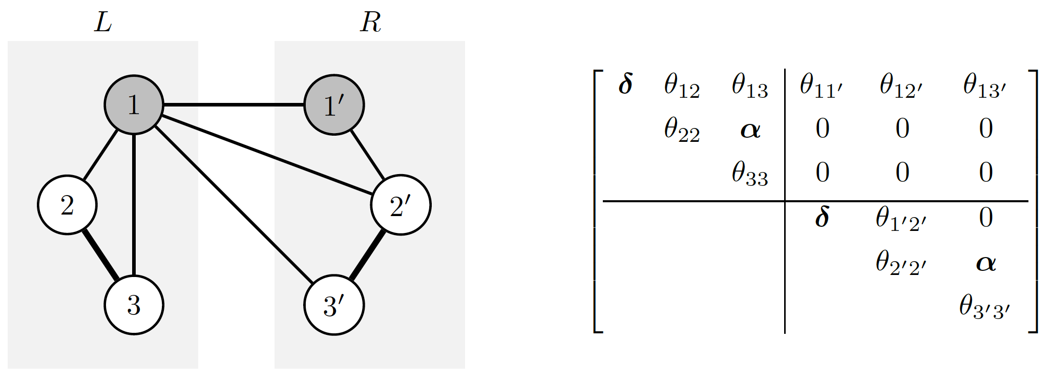
Figure C.1: Coloured graph and concentration matrix of the pdRCON model in Example C.1

In the pdRCON model of Figure C.1 the edges $\{2,3\}\in\mathcal{G}_{L}$ and $\{2^{\prime},3^{\prime}\}\in\mathcal{G}_{R}$ are both present and such that $\theta_{23}=\theta_{2^{\prime}3^{\prime}}=\alpha$; that is, they form an inside-block parametric symmetry. On the other hand the edges $\{1,2\}\in\mathcal{G}_{L}$ and $\{1^{\prime},2^{\prime}\}\in\mathcal{G}_{R}$ are both present, thereby forming an inside-block structural symmetry, but not a parametric symmetry because the corresponding concentrations $\theta_{12}$ and $\theta_{1^{\prime}2^{\prime}}$ are not constrained to be equal. In this model there is also one vertex symmetry, encoded by the equality constraints $\theta_{11}=\theta_{1^{\prime}1^{\prime}}=\delta$, whereas the only existing across-block symmetries are those that involve missing edges, and thus zero concentrations. ∎

Example C.2 (Figure C.2).

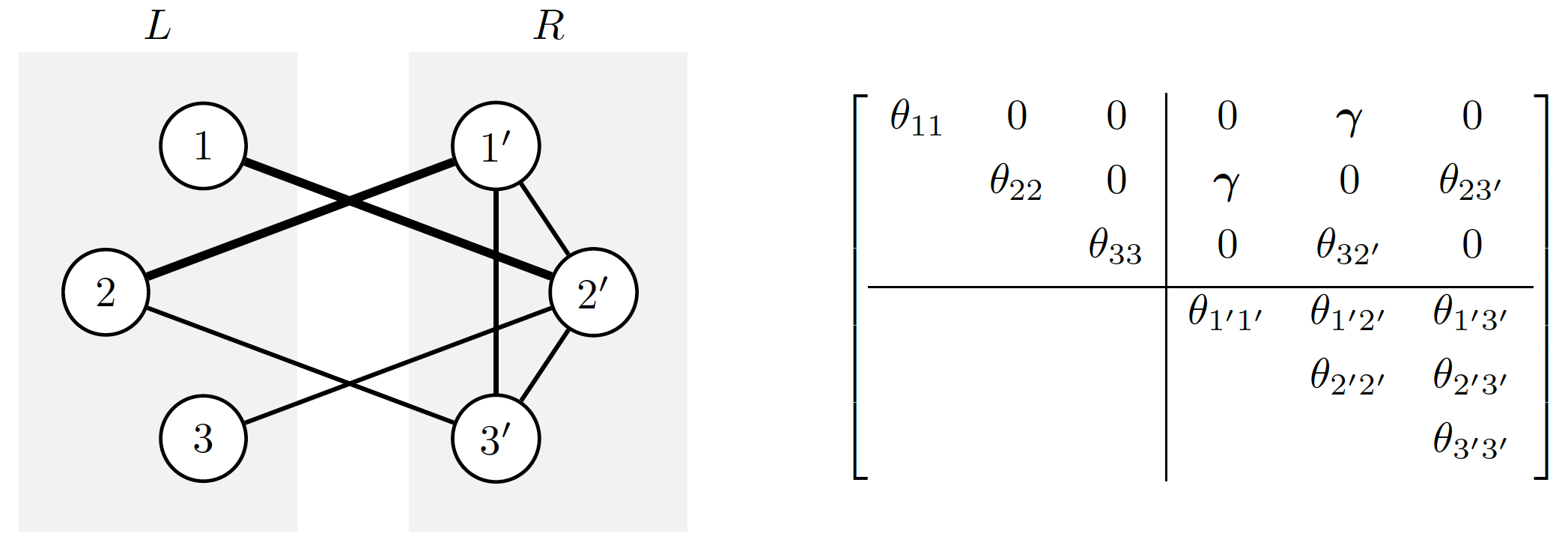
Figure C.2: Coloured graph and concentration matrix of the pdRCON model in Example C.2

In the pdRCON model of Figure C.2 the edges $\{1,2^{\prime}\}$ and $\{2,1^{\prime}\}$ are both present and form the inside-block parametric symmetry $\theta_{12^{\prime}}=\theta_{21^{\prime}}=\gamma$. On the other hand, the edges $\{2,3^{\prime}\}$ and $\{3,2^{\prime}\}$ edges are both present, thereby forming an across-block structural symmetry, but not a parametric symmetry because the corresponding concentrations $\theta_{23^{\prime}}$ and $\theta_{32^{\prime}}$ are not constrained to be equal. In this model, there are neither vertex symmetries nor inside-block symmetries. Indeed, the inner structure of the two groups is very different because $\mathcal{G}_{L}$ is a fully disconnected whereas $\mathcal{G}_{R}$ is complete. ∎

Example C.3 (Figure C.3).

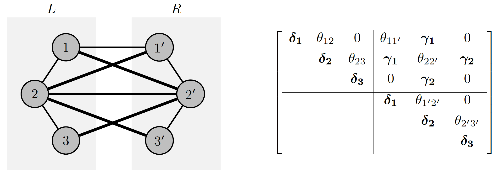
Figure C.3: Coloured graph and concentration matrix of the pdRCON model in Example C.3

The pdRCON model of Figure C.3 shows a large amount of symmetry. More specifically, there is (i) full vertex symmetry with $\theta_{11}=\theta_{1^{\prime}1^{\prime}}=\delta_{1}$ $\theta_{22}=\theta_{2^{\prime}2^{\prime}}=\delta_{2}$ $\theta_{33}=\theta_{3^{\prime}3^{\prime}}=\delta_{3}$; (ii) full across-block parametric symmetry with $\theta_{12^{\prime}}=\theta_{21^{\prime}}=\gamma_{1}$ and $\theta_{23^{\prime}}=\theta_{3^{\prime}2}=\gamma_{2}$ and, finally, (iii) there is full inside-block structural symmetry. However, there are no inside-block parametric symmetries involving present edges, and therefore this is not a fully symmetric model. ∎

Example C.4 (Figure C.4).

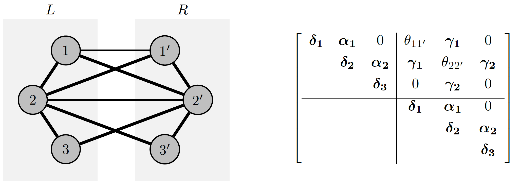
Figure C.4: Coloured graph and concentration matrix of the pdRCON model in Example C.4

The structure of the graph in Figure C.4 is the same as that considered in Example C.3, but in this case there are additional equality constraints so that full parametric symmetry is achieved. In may be worth noting that, although this is a fully symmetric model, thin lines are used to depict the edges $\{1,1^{\prime}\}$ and $\{2,2^{\prime}\}$. Indeed, these edges are associated with the diagonal entries of $\Theta_{LR}$ and, in pdRCON models, these parameters are not considered for possible equality constraints. ∎

Appendix D ADMM algorithm

We provide here an ADMM algorithm for the solution of the optimization problem in (7), as implemented in the R package pdglasso; see also Danaher et al. (2014) and Ranciati et al. (2021). Following Boyd et al. (2011), the problem is stated as the optimization with respect to $\Theta\in\mathcal{S}^{+}$ and $Z\in\mathcal{S}^{+}$ of the quantity,

$$-\log\det(\Theta)+\operatorname{tr}(S\Theta)+\mathcal{P}_{\lambda_{1}}(Z)+\mathcal{Q}_{\lambda_{2}}(Z),$$

under the constraints $Z=\Theta$. Hence, from (9), the (scaled form) augmented Lagrangian (see Boyd et al., 2011, Section 3.1.1) of the optimization problem can be written as

$$\text{L}_{\rho_{1}}\bigl{(}\Theta,Z,U\bigl{)}= -\log\det(\Theta)+\operatorname{tr}(S\Theta)+\mathcal{P}_{\lambda_{1}}(Z)+\mathcal{Q}_{\lambda_{2}}(Z)+\dfrac{\rho_{1}}{2}\left\lVert\Theta-Z+U\right\rVert^{2}_{\text{F}}-\dfrac{\rho_{1}}{2}\left\lVert U\right\rVert^{2}_{\text{F}}=$$

$$-\log\det(\Theta)+\operatorname{tr}(S\Theta)+\lambda_{1}\!\left\lVert Z\right\rVert_{1}+\lambda_{2}^{(V)}\left\lVert\operatorname{diag}(Z_{LL})-\operatorname{diag}(Z_{RR})\right\rVert_{1}+$$

$$+\lambda_{2}^{(I)}\left\lVert Z_{LL}^{\ast}-Z_{RR}^{\ast}\right\rVert_{1}+\lambda_{2}^{(A)}\left\lVert Z_{LR}-Z_{RL}\right\rVert_{1}+\dfrac{\rho_{1}}{2}\left\lVert\Theta-Z+U\right\rVert^{2}_{\text{F}}-\dfrac{\rho_{1}}{2}\left\lVert U\right\rVert^{2}_{\text{F}},$$ (D.1)

where $U$ is the scaled dual variable, $\left\lVert\cdot\right\rVert_{\text{F}}$ denotes the Frobenius norm and $\rho_{1}>0$ is the step size.

Equation (D) is then optimized by looping, over iterations $l=1,2,\dots$, the following three steps (see Boyd et al., 2011, equations (3.5) to (3.6)):

1. $\displaystyle\Theta^{l+1}:=\operatorname*{arg\,min}_{\Theta}\left(-\log\det(\Theta)+\operatorname{tr}(S\Theta)+\dfrac{\rho_{1}}{2}\left\lVert\Theta-Z^{l}+U^{l}\right\rVert^{2}_{\text{F}}\right);$

2. $\displaystyle Z^{l+1}:=\underset{Z}{\operatorname*{arg\,min}}\biggl{(}\mathcal{P}_{\lambda_{1}}(Z)+\mathcal{Q}_{\lambda_{2}}(Z)+\dfrac{\rho_{1}}{2}\left\lVert\Theta^{l+1}-Z+U^{l}\right\rVert^{2}_{\text{F}}\biggl{)};$

3. $\displaystyle U^{l+1}:=U^{l}+\Theta^{l+1}-Z^{l+1}.$

The solution to step (1) can be obtained in analytic form as detailed in Boyd et al. (2011, Section 3.1.1); see also Ranciati et al. (2021).

More specific of our implementation is the solution of step (2). Consider a matrix $Q$ whose columns and rows are indexed by $V=L\cup R$, the half-vectorization operator $\operatorname{vech}(\cdot)$, and the diagonal extraction operator $\operatorname{vd}(\cdot)$. We define the vector $\operatorname{v}(Q)$ to be:

$$\operatorname{v}(Q)^{\top}=\left[\begin{array}[]{ccccccc}\operatorname{vd}(Q_{LL})^{\top}&\operatorname{vd}(Q_{RR})^{\top}&\operatorname{vech}(Q_{LL})^{\top}&\operatorname{vech}(Q_{RR})^{\top}&\operatorname{vech}(Q_{LR})^{\top}&\operatorname{vech}(Q_{RL})^{\top}&\operatorname{vd}(Q_{LR})^{\top}\end{array}\right],$$

and we set $z^{l}=\operatorname{v}(Z^{l}),$ $b^{l}=\operatorname{v}(\Theta^{l})+\operatorname{v}(U^{l})$. All (linear) equality constraints are encoded in the matrix $F$, built as

$$F=\left[\begin{array}[]{ccccccc}I_{q}&-I_{q}&O_{qs}&O_{qs}&O_{qs}&O_{qs}&O_{qq}\\ O_{sq}&O_{sq}&I_{s}&-I_{s}&O_{ss}&O_{ss}&O_{sq}\\ O_{sq}&O_{sq}&O_{ss}&O_{ss}&I_{s}&-I_{s}&O_{qq}\\ \end{array}\right]$$

where $I$ and $O$ are respectively the identity and zero matrix, with $s=q(q-1)/2$. Thus, step (2) can be stated as a self standing optimization problem,

$$\operatorname*{arg\,min}_{z}\biggl{(}\dfrac{1}{2}\left\lVert z-b\right\rVert^{2}_{2}+\lambda^{\prime}_{1}\!\left\lVert z\right\rVert_{1}+\left\lVert F(\bm{\lambda}^{\prime}_{2}\circ z)\right\rVert_{1}\biggl{)},$$

where: $\circ$ is the element-wise product, $\lambda^{\prime}_{1}=\lambda_{1}/\rho_{1},$ ${\bm{\lambda}^{\prime}}^{\top}_{2}=\left[\dfrac{\lambda_{2}^{(V)}}{\rho_{1}}{\bm{1}_{2q}}^{\top}\,\,\,\,\,\dfrac{\lambda_{2}^{(I)}}{\rho_{1}}{\bm{1}_{2s}}^{\top}\,\,\,\,\,\dfrac{\lambda_{2}^{(A)}}{\rho_{1}}{\bm{1}_{2s+q}}^{\top}\right],$ and $\bm{1}_{q}$ the unit vector of length $q$. Due to Friedman et al. (2007, Lemma A.1), we can solve

$$\operatorname*{arg\,min}_{z}\biggl{(}\dfrac{1}{2}\left\lVert z-b\right\rVert^{2}_{2}+\left\lVert F(\bm{\lambda}^{\prime}_{2}\circ z)\right\rVert_{1}\biggl{)},$$

with $\lambda^{\prime}_{1}=0$ and obtain the solution for the case $\lambda^{\prime}_{1}>0$ via a soft-thresholding operation. This is a generalized lasso problem (Tibshirani and Taylor, 2011), which we solve with the following inner ADMM procedure (Boyd et al., 2011, Section 6.4.1):

1. $z^{m+1}:=\bigl{(}I+\rho_{2}F^{\top}\!F\bigl{)}^{-1}\left\{b+\rho_{2}F^{\top}\!(v^{m}-t^{m})\right\}$;

2. $v^{m+1}:=\mathcal{S}_{\bm{\lambda}^{\prime}_{2}/\rho_{2}}(Fz^{m+1}+t^{m})$;

3. $t^{m+1}:=t^{m}+Fz^{m+1}-v^{m+1}$.

The stopping rule of the algorithm is based on the primal and dual residual (Boyd et al., 2011, Section 3.3.1), computed at each iteration, which are compared to numerical precision thresholds that matrix values at convergence should achieve.

Finally, we remark that, in the computer implementation of the above ADMM algorithm, efficiency has been achieved by making the step sizes $\rho_{1}$ and $\rho_{2}$ adaptive, and by encoding the results of the products involving the matrix $F$ in the form of less expensive vectorized computations, explicitly based on the (sparse) structure of such matrix.

Appendix E Plots of the two selected models for the breast cancer analysis of Section 6

Visual depiction of the two graphs associated to: (i) pdRCON model with forced full vertex symmetry and penalization on inside- and across- blocks (mod${}_{\text{fV}}$, Figure E.1); (ii) fully symmetric pdRCON model (mod${}_{\text{fVIA}}$, Figure E.2). In both plots, the character coding is the following: empty circle, for structural non-zero symmetries (unicode character U+25CB, white circle); full circle, for parametric non-zero symmetries (unicode character U+25CF, black circle); diagonal slash for asymmetric edges (unicode character U+2571, box drawings light diagonal upper right to lower left). Labels for columns and rows end with the string “_T” if the genes are measured on tumor tissues and “_H” if measured on healthy tissues. Lower triangular portion is not shown due to the symmetric nature of the matrix.

Figure E.1: Depiction of the graph associated to model mod${}_{\text{fV}}$, selected according to eBIC ($\gamma=0.5$), and fit on the breast cancer data of Section 6; for row and column labels, “_T” denotes tumor tissue and “_H” healthy tissue; character coding: empty circle, structural non-zero symmetries; full circle, parametric non-zero symmetries; diagonal slash, asymmetric edges.

Figure E.2: Depiction of the graph associated to model mod${}_{\text{fVIA}}$ (fully symmetric model), selected according to eBIC ($\gamma=0.5$), and fit on the breast cancer data of Section 6; for row and column labels, “_T” denotes tumor tissue and “_H” healthy tissue; character coding: empty circle, structural non-zero symmetries; full circle, parametric non-zero symmetries; diagonal slash, asymmetric edges.

References

- Aran et al. (2017) Aran, D., R. Camarda, J. Odegaard, H. Paik, B. Oskotsky, G. Krings, A. Goga, M. Sirota, and A. J. Butte (2017). Comprehensive analysis of normal adjacent to tumor transcriptomes. Nature communications 8(1), 1–14.
- Boyd et al. (2011) Boyd, S., N. Parikh, E. Chu, B. Peleato, and J. Eckstein (2011). Distributed optimization and statistical learning via the alternating direction method of multipliers. Foundations and Trends® in Machine learning 3(1), 1–122.
- Danaher et al. (2014) Danaher, P., P. Wang, and D. M. Witten (2014). The joint graphical lasso for inverse covariance estimation across multiple classes. Journal of the Royal Statistical Society: Series B (Statistical Methodology) 76(2), 373–397.
- Foygel and Drton (2010) Foygel, R. and M. Drton (2010). Extended bayesian information criteria for gaussian graphical models. In Advances in neural information processing systems, pp. 604–612.
- Friedman et al. (2007) Friedman, J., T. Hastie, H. Höfling, and R. Tibshirani (2007). Pathwise coordinate optimization. The Annals of Applied Statistics 1(2), 302–332.
- Friedman et al. (2008) Friedman, J., T. Hastie, and R. Tibshirani (2008). Sparse inverse covariance estimation with the graphical lasso. Biostatistics 9(3), 432–441.
- Gehrmann (2011) Gehrmann, H. (2011). Lattices of graphical Gaussian models with symmetries. Symmetry 3(3), 653–679.
- Graczyk et al. (2022) Graczyk, P., H. Ishi, B. Kołodziejek, and H. Massam (2022). Model selection in the space of Gaussian models invariant by symmetry. The Annals of Statistics 50(3), 1747–1774.
- Hoefling (2010) Hoefling, H. (2010). A path algorithm for the fused lasso signal approximator. Journal of Computational and Graphical Statistics 19(4), 984–1006.
- Højsgaard and Lauritzen (2008) Højsgaard, S. and S. L. Lauritzen (2008). Graphical Gaussian models with edge and vertex symmetries. Journal of the Royal Statistical Society: Series B (Statistical Methodology) 70(5), 1005–1027.
- Højsgaard et al. (2007) Højsgaard, S., S. L. Lauritzen, et al. (2007). Inference in graphical Gaussian models with edge and vertex symmetries with the gRc package for R. Journal of Statistical Software 23(6), 1–26.
- Kubo et al. (2004) Kubo, M., M. Nakamura, A. Tasaki, N. Yamanaka, H. Nakashima, M. Nomura, S. Kuroki, and M. Katano (2004). Hedgehog signaling pathway is a new therapeutic target for patients with breast cancer. Cancer research 64(17), 6071–6074.
- Lauritzen (1996) Lauritzen, S. L. (1996). Graphical models. Oxford University Press.
- Lütkepohl (1996) Lütkepohl, H. (1996). Handbook of Matrices. New York: John Wiley and Sons.
- Mazumder and Hastie (2012) Mazumder, R. and T. Hastie (2012). Exact covariance thresholding into connected components for large-scale graphical lasso. Journal of Machine Learning Research 13(27), 781–794.
- R Core Team (2023) R Core Team (2023). R: A Language and Environment for Statistical Computing. Vienna, Austria: R Foundation for Statistical Computing.
- Ranciati et al. (2021) Ranciati, S., A. Roverato, and A. Luati (2021). Fused graphical lasso for brain networks with symmetries. Journal of the Royal Statistical Society: Series C (Applied Statistics) 70(5), 1299–1322.