Solitons to Mean Curvature Flow
in the hyperbolic $3$-space

Abstract.

We consider translators (i.e., initial condition of translating solitons) to mean curvature flow (MCF) in the hyperbolic $3$-space $\mathbb{H}^{3}$, providing existence and classification results. More specifically, we show the existence and uniqueness of two distinct one-parameter families of complete rotational translators in $\mathbb{H}^{3},$ one containing catenoid-type translators, and the other parabolic cylindrical ones. We establish a tangency principle for translators in $\mathbb{H}^{3}$ and apply it to prove that properly immersed translators to MCF in $\mathbb{H}^{3}$ are not cylindrically bounded. As a further application of the tangency principle, we prove that any horoconvex translator which is complete or transversal to the $x_{3}$-axis is necessarily an open set of a horizontal horosphere. In addition, we classify all translators in $\mathbb{H}^{3}$ which have constant mean curvature. We also consider rotators (i.e., initial condition of rotating solitons) to MCF in $\mathbb{H}^{3}$ and, after classifying the rotators of constant mean curvature, we show that there exists a one-parameter family of complete rotators which are all helicoidal, bringing to the hyperbolic context a distinguished result by Halldorsson, set in $\mathbb{R}^{3}.$

2020 Mathematics Subject Classification: 53E10 (primary), 53E99 (secondary).

Key words and phrases: soliton – mean curvature flow – hyperbolic space – invariant surfaces.

1. Introduction

The last decades flourished with great regard to the theory of extrinsic geometric flows in Riemannian manifolds, especially to mean curvature flow in Euclidean spaces, giving rise to a vast literature on the subject (cf. [2] and the references therein). Extrinsic geometric flows constitute evolution equations that describe hypersurfaces of a Riemannian manifold evolving in the normal direction with velocity given by the corresponding extrinsic curvature. A special class of solutions is that of the solitons, also known as the self-similar solutions, which are characterized for being generated by the Killing field defined by a one-parameter subgroup of isometries of the ambient manifold. When these isometries are translations along a geodesic, we call the corresponding self-similar solutions translating solitons to the giving flow, and the initial hypersurfaces are known as translators. A main feature of translators in Euclidean spaces is that they naturally appear as type II singularities of certain compact solutions to mean curvature flow (cf. [12, Theorem 4.1]).

There exist many examples of translators to mean curvature flow (MCF, for short) in Euclidean space $\mathbb{R}^{3}.$ Three of the best known are the cylinder over the graph of the function $f(t)=-\log(\cos t),$ $t\in(-\pi/2,\pi/2),$ called the grim reaper, the rotational entire graph over $\mathbb{R}^{2}$ obtained by Altschuler and Wu [1] known as the translating paraboloid or bowl soliton, and the one-parameter family of rotational annuli obtained by Clutterbuck, Schnürer and Schulze [6], the so called translating catenoids. On the other hand, little is known about translators in hyperbolic spaces.

In this paper, we consider solitons to MCF in hyperbolic space $\mathbb{H}^{3}$, and first we focus on the case of translators which move by hyperbolic translations along a fixed geodesic. We classify all such surfaces with constant mean curvature (Theorems 3.2 and 3.4) and also obtain new families of examples (see Figure 1), which, by some similarities with the translators in $\mathbb{R}^{3}$ described above, will be called the translating catenoid (Theorem 3.9) and the grim reaper (Theorem 3.13). These translators are then proven to be unique with respect to their fundamental properties (Theorems 3.10 and 3.16).

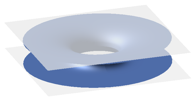
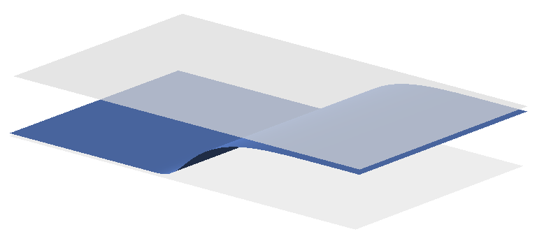
Figure 1. A translating catenoid and a grim reaper in the half-space model of $\mathbb{H}^{3}$.

A main tool in establishing uniqueness results for translators in Euclidean space is the tangency principle. It asserts that two such translators which are tangent at a point, with one on one side of the other in a neighborhood of this point, must coincide in this neighborhood. In fact, this result is a direct consequence of the tangency principle for minimal surfaces, since translators in Euclidean space become minimal surfaces when the ambient space is endowed with a suitable metric (cf. Section 3.3). Apparently, for translators in hyperbolic space, such a metric is not available. Nevertheless, we prove that a tangency principle holds for translators in $\mathbb{H}^{3}$ as well (Theorem 3.17). Then, by using the family of translating catenoids as barriers, we apply it to prove that properly immersed translators in $\mathbb{H}^{3}$ are never cylindrically bounded and, in particular, never closed. As a further application, we show that any horoconvex translator which is complete or transversal to the axis of the translation is necessarily an open set of a horosphere (Theorem 3.20).

We study, as well, rotators to MCF, that is, initial data of solitons whose associated isometries are rotations around a geodesic. In [10], Halldorsson considered rotators in $\mathbb{R}^{3},$ obtaining a one-parameter family of complete helicoidal rotators in $\mathbb{R}^{3}$ which are also translators. Inspired by Halldorsson’s work, we obtain here an analogous result (Theorem 4.4), in which we construct a one-parameter family of helicoidal surfaces in $\mathbb{H}^{3}$ that, under mean curvature flow, rotates around its axis and translates downwards with velocity that equals its pitch, see Figure 2. As in the case of translators, we also classify all rotators of constant mean curvature in $\mathbb{H}^{3}$ (Theorem 4.1).

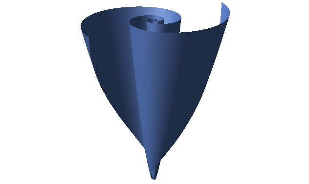
Figure 2. A helicoidal rotational soliton.

The paper is organized as follows. In Section 2, we set some notation and formulae. In Section 3, we introduce translators to MCF in $\mathbb{H}^{3}$ and establish the aforementioned results related to them. In Section 4 we deal with rotators to MCF in $\mathbb{H}^{3}.$ Finally, we use Section 5 to present the classification of minimal translators in $\mathbb{H}^{3}$.

Acknowledgments.

We heartily thank Eric Toubiana for pointing us to the existence result necessary for the final argument in Section 5, and also Marcus Marrocos, for the enlightening conversations that led to the proofs of Lemmas 3.7 and 3.12.

2. Preliminaries

Throughout the paper, we shall consider the upper half-space model of $\mathbb{H}^{3},$ that is, $\mathbb{H}^{3}:=(\mathbb{R}_{+}^{3},ds^{2}),$ where $\mathbb{R}^{3}_{+}=\{(x_{1},x_{2},x_{3})\in\mathbb{R}^{3}\mid x_{3}>0\}$, $ds^{2}:={d\bar{s}^{2}}/{x_{3}^{2}}$ and $d\bar{s}^{2}$ is the standard Euclidean metric of $\mathbb{R}_{+}^{3}.$ We will also denote $ds^{2}$ by $\langle\,,\,\rangle.$

Let $\varSigma$ be an oriented surface in a Riemannian 3-manifold $\overline{M}$. Set $\overline{\nabla}$ for the Levi-Civita connection of $\overline{M},$ $\eta$ for the unit normal field of $\varSigma,$ and $A$ for its shape operator with respect to $\eta,$ so that

$$AX=-\overline{\nabla}_{X}\eta,\,\,X\in T\varSigma,$$

where $T\varSigma$ stands for the tangent bundle of $\varSigma$. The principal curvatures of $\varSigma,$ that is, the eigenvalues of $A,$ will be denoted by $k_{1},k_{2}$ and the mean curvature $H$ of $\varSigma$ is expressed by

$$H=\frac{k_{1}+k_{2}}{2}.$$

The mean curvature vector of $\varSigma$ is

$$\mathbf{H}=H\eta,$$

which is invariant under the choice of orientation $\eta\to-\eta$ and satisfies $\|\mathbf{H}\|=|H|$.

Given an oriented surface $\varSigma\subset\mathbb{R}_{+}^{3},$ let $\bar{\eta}=(\bar{\eta}_{1},\bar{\eta}_{2},\bar{\eta}_{3})$ be the unit normal of $\varSigma$ with respect to the induced Euclidean metric $d\bar{s}^{2}.$ It is easily checked that

$$\eta(p)=x_{3}\bar{\eta}(p),\,\,\,p=(x_{1},x_{2},x_{3})\in\varSigma$$

defines a unit normal of $\varSigma$ with respect to the hyperbolic metric $ds^{2}.$ With these orientations, if we denote by $\mkern 1.5mu\overline{\mkern-1.5muH\mkern-1.5mu}\mkern 1.5mu$ (resp. $H$) the mean curvature of $\varSigma$ with respect to the Euclidean metric (resp. hyperbolic metric) of $\mathbb{R}_{+}^{3},$ we have that $\mkern 1.5mu\overline{\mkern-1.5muH\mkern-1.5mu}\mkern 1.5mu$ and $H$ satisfy the following relation (cf. [15, Lemma 10.1.1]):

(1) $$H(p)=x_{3}\mkern 1.5mu\overline{\mkern-1.5muH\mkern-1.5mu}\mkern 1.5mu(p)+\bar{\eta}_{3}(p)\,\,\,\forall p=(x_{1},x_{2},x_{3})\in\varSigma.$$

2.1. Mean curvature flow

We say that a family of oriented surfaces $\varSigma_{t}=X_{t}(M)$ of a Riemannian $3$-manifold $\mkern 1.5mu\overline{\mkern-1.5muM\mkern-1.5mu}\mkern 1.5mu$ evolves under mean curvature flow if the corresponding one-parameter family of immersions

$$X_{t}\colon M\rightarrow\mkern 1.5mu\overline{\mkern-1.5muM\mkern-1.5mu}\mkern 1.5mu,\,\,\,t\in[0,\delta),\,\,\,0<\delta\leq+\infty,$$

satisfies the following condition:

(2) $$\frac{\partial X_{t}}{\partial t}^{\perp}(p)=H_{t}(p)\eta_{t}(p)\,\,\,\forall p\in M,$$

where $\eta_{t}$ is the unit normal to $X_{t},$ $H_{t}$ is the mean curvature of $X_{t}$ with respect to $\eta_{t},$ and $\frac{\partial X_{t}}{\partial t}^{\perp}$ denotes the normal component of $\frac{\partial X_{t}}{\partial t},$ that is,

$$\frac{\partial X_{t}}{\partial t}^{\perp}=\left\langle\frac{\partial X_{t}}{\partial t},\eta_{t}\right\rangle\eta_{t}\,.$$

In particular, the equality (2) is equivalent to

$$\left\langle\frac{\partial X_{t}}{\partial t},\eta_{t}\right\rangle=H_{t}.$$

We call such a family $X_{t}:M\rightarrow\mkern 1.5mu\overline{\mkern-1.5muM\mkern-1.5mu}\mkern 1.5mu,$ $t\in[0,\delta)$ a mean curvature flow (MCF, for short) in $\mkern 1.5mu\overline{\mkern-1.5muM\mkern-1.5mu}\mkern 1.5mu$ with initial data $X_{0}.$ In this setting, we say that $\varSigma_{t}=X_{t}(M)$ is a soliton or a self-similar solution to MCF if there exists a one-parameter subgroup $\mathcal{G}:=\{\Gamma_{t}\mid t\in\mathbb{R}\}$ of the group of isometries of $\mkern 1.5mu\overline{\mkern-1.5muM\mkern-1.5mu}\mkern 1.5mu,$ such that $\Gamma_{0}$ is the identity map of $\mkern 1.5mu\overline{\mkern-1.5muM\mkern-1.5mu}\mkern 1.5mu$ and

$$\varSigma_{t}=\Gamma_{t}(\varSigma)\,\,\,\forall t\in\mathbb{R}$$

is a MCF. More specifically, we shall call such a family $\varSigma_{t}$ a $\mathcal{G}$-soliton.

Let $\xi$ be the Killing field determined by the subgroup $\mathcal{G},$ i.e., for any $p\in\mkern 1.5mu\overline{\mkern-1.5muM\mkern-1.5mu}\mkern 1.5mu,$

$$\xi(p):=\frac{\partial}{\partial t}\Gamma_{t}(p)\,\,\,\,\,\text{at}\,\,\,t=0.$$

It can be proved (see, e.g., [13]) that the surface $\varSigma=X_{0}(M)$ with unit normal $\eta$ is the initial condition of a $\mathcal{G}$-soliton generated by $\xi$ in $\mkern 1.5mu\overline{\mkern-1.5muM\mkern-1.5mu}\mkern 1.5mu$ if and only if the equality

(3) $${H=\langle\xi,\eta\rangle}$$

holds everywhere on $\varSigma.$ So, in the class of solitons, equation (2) is in fact a prescribed mean curvature problem.

3. Translators to MCF in $\mathbb{H}^{3}$

Consider in hyperbolic space $\mathbb{H}^{3}$ the group $\mathcal{G}=\{\Gamma_{t}\mid t\in\mathbb{R}\}\subset{\rm Iso}(\mathbb{H}^{3})$ of hyperbolic translations along the $x_{3}$-axis, defined by

$$\Gamma_{t}(p)=e^{t}p,\,\,\,p\in\mathbb{H}^{3}.$$

In this setting, an initial condition of a $\mathcal{G}$-soliton will be called a translating soliton or simply a translator. Using the abuse of notation

$$p=(x_{1},x_{2},x_{3})\in\mathbb{H}^{3}\leftrightarrow x_{1}\partial_{x_{1}}+x_{2}\partial_{x_{2}}+x_{3}\partial_{x_{3}}\in T_{p}\mathbb{H}^{3},$$

the Killing field associated to $\mathcal{G}$ is $\xi(p)=p,$ $p\in\mathbb{H}^{3}$. Thus, it follows from (3) that a surface $\varSigma\subset\mathbb{H}^{3}$ is a translator to MCF if and only if

(4) $$H(p)=\langle p,\eta(p)\rangle\,\,\,\forall p\in\varSigma.$$

Example 3.1.

Let $\Pi$ be a totally geodesic vertical plane of $\mathbb{H}^{3}$ which contains $(0,0,1)$. Since $H$ vanishes on $\Pi$, it is clear that (4) holds for $\varSigma=\Pi.$ Thus, $\Pi$ is a stationary translator to MCF in $\mathbb{H}^{3}.$

In fact, equation (3) implies that a minimal surface $\varSigma\subset\mathbb{H}^{3}$ is a (stationary) translator to MCF if and only if it is invariant under the group $\mathcal{G}$ of hyperbolic isometries as above. A complete classification of such surfaces is given by the following description.

Theorem 3.2.

There exists a one-parameter family $\varSigma_{\theta}$, $\theta\in(0,\pi],$ of properly embedded minimal surfaces in $\mathbb{H}^{3}$ with the following properties:

• $\varSigma_{\theta}$ is invariant under the one-parameter group $\{\Gamma_{t}\}_{t\in\mathbb{R}}$ of hyperbolic translations

  $${p\in\mathbb{H}^{3}\mapsto\Gamma_{t}(p):=e^{t}p\in\mathbb{H}^{3},}$$

  and so it is a stationary translator to MCF in $\mathbb{H}^{3}.$

• $\partial_{\infty}\varSigma_{\theta}\cap\mathbb{R}^{2}$ is the union of two half-lines making an angle $\theta.$

• $\varSigma_{\pi}$ is a vertical plane.

Conversely, if $\varSigma$ is a properly embedded minimal surface of  $\mathbb{H}^{3}$ which is invariant under the group $\Gamma_{t},$ then $\varSigma=\varSigma_{\theta}$ for some $\theta\in(0,\pi].$

The proof of Theorem 3.2, for convenience, will be presented separately in Section 5. Concerning the case of translators with nonzero constant mean curvature, we start with the next example.

Example 3.3.

Let $\mathscr{H}_{h}$ be the horosphere of $\mathbb{H}^{3}=(\mathbb{R}^{3}_{+}\,,\,ds^{2})$ at height $h>0,$ i.e.,

$$\mathscr{H}_{h}=\{(x_{1},x_{2},h)\in\mathbb{H}^{3}\mid x_{1},x_{2}\in\mathbb{R}\}.$$

At any point $p=(x_{1},x_{2},h)\in\mathscr{H}_{h},$ we have that $H(p)=1$ and $\eta(p)=he_{3},$ so that

$$\langle p,\eta(p)\rangle=\frac{1}{h^{2}}h^{2}=1=H(p)\,\,\ \forall p\in\mathscr{H}_{h}.$$

Hence, $\mathscr{H}_{h}$ is a translator to MCF in $\mathbb{H}^{3}.$

In our next result we show that horospheres are the only translators to MCF which have nonzero constant mean curvature. In the proof, we shall use the following evolution formula for the mean curvature $H_{t}$ (notation as in Section 2) of a mean curvature flow $X_{t}:M\to\mkern 1.5mu\overline{\mkern-1.5muM\mkern-1.5mu}\mkern 1.5mu$:

(5) $$\frac{\partial H_{t}}{\partial t}=\Delta H_{t}+H_{t}(\|A_{t}\|^{2}+\mkern 1.5mu\overline{\mkern-1.5mu\rm Ric\mkern-1.5mu}\mkern 1.5mu(\eta_{t},\eta_{t})),$$

where $\mkern 1.5mu\overline{\mkern-1.5mu\rm Ric\mkern-1.5mu}\mkern 1.5mu$ denotes the Ricci tensor of $\mkern 1.5mu\overline{\mkern-1.5muM\mkern-1.5mu}\mkern 1.5mu$ (see [11, Theorem 3.2-(v)]).

Theorem 3.4.

Let $\varSigma$ be a connected translator to MCF in $\mathbb{H}^{3}$ which has nonzero constant mean curvature. Then, $\varSigma$ is an open subset of a horosphere.

Proof.

After a change of orientation, we may assume without loss of generality that the mean curvature $H$ of $\varSigma$ is positive. Let $X_{t}:M\to\mathbb{H}^{3},$ $t>0,$ be the MCF such that $X_{0}(M)=\varSigma$ and

$$X_{t}(p)=e^{t}X_{0}(p),\,\,\,p\in M.$$

Since $X_{t}(M)$ differs from $X_{0}(M)$ by an ambient isometry, $H_{t}=H>0$ is constant in space and time, thus ${\partial H_{t}}/{\partial t}=\Delta H_{t}=0.$ Also, in $\mathbb{H}^{3},$ $\mkern 1.5mu\overline{\mkern-1.5mu\rm Ric\mkern-1.5mu}\mkern 1.5mu(\eta_{t},\eta_{t})=-2.$ Then, formula (5) yields $\|A_{t}\|^{2}=2$ for all $t\geq 0.$ Taking $t=0,$ we conclude that the principal curvatures $k_{1},k_{2}$ of $\varSigma$ satisfy:

$${\left\{\begin{array}[]{cccccl}k_{1}&+&k_{2}&=&2H,\\[4.30554pt] k_{1}^{2}&+&k_{2}^{2}&=&2,\end{array}\right.}$$

from where it follows that $H\in(0,1]$ and, after possibly reindexing,

$${k_{1}=H+\sqrt{1-H^{2}},\quad k_{2}=H-\sqrt{1-H^{2}}.}$$

Since $H$ is constant, both $k_{1}$ and $k_{2}$ are constant, so $\varSigma$ is isoparametric. The isoparametric surfaces of $\mathbb{H}^{3}$ are classified (see [3, Theorem 3.14]) and the fact that $H\in(0,1]$ imply that $\varSigma$ is either an open subset of a horosphere or of an equidistant surface to a totally geodesic plane. However, $k_{1}^{2}+k_{2}^{2}=2$ only holds when $\varSigma$ is contained in a horosphere, which finishes the proof of the theorem. ∎

Remark 3.5.

Since (5) holds for any $\mathcal{G}$-soliton, the proof of Theorem 3.4 applies to show that any initial condition of a $\mathcal{G}$-soliton in $\mathbb{H}^{3}$ with nonzero constant mean curvature is necessarily an open subset of a horosphere.

3.1. Rotational translators.

In this section, we focus on translators to MCF in $\mathbb{H}^{3}$ which are invariant under rotations about the $x_{3}$-axis. With this purpose, we first consider vertical rotational graphs. More precisely, let $\phi$ be a positive smooth function on an open interval $I\subset(0,+\infty),$ and assume its graph $\varSigma$ in $\mathbb{H}^{3}$ is invariant under rotations about the $x_{3}$-axis. Then, $\varSigma$ admits a parameterization of the form

$$X(u,v)=(v\cos u,v\sin u,\phi(v)),\,\,\,\,(u,v)\in U:=\mathbb{R}\times I\subset\mathbb{R}^{2}.$$

We shall call $\varSigma=X(U)$ the rotational vertical graph determined by $\phi.$

For a rotational graph $\varSigma$ as above, a direct computation gives that

$$\bar{\eta}:=(\bar{\eta}_{1},\bar{\eta}_{2},\bar{\eta}_{3})=\varrho(-\phi^{\prime}\cos u,-\phi^{\prime}\sin u,1),\quad\varrho:=\frac{1}{\sqrt{1+(\phi^{\prime}))^{2}}},$$

is a unit normal with respect to the induced Euclidean metric, and that the corresponding Euclidean mean curvature is

$$\mkern 1.5mu\overline{\mkern-1.5muH\mkern-1.5mu}\mkern 1.5mu=\frac{\varrho}{2}\left(\frac{\phi^{\prime\prime}}{1+(\phi^{\prime})^{2}}+\frac{\phi^{\prime}}{v}\right).$$

Thus, from (1), the mean curvature $H$ of $\varSigma$ in $\mathbb{H}^{3}$ with respect to $\eta:=\phi\bar{\eta}$ is

(6) $$H=\phi\mkern 1.5mu\overline{\mkern-1.5muH\mkern-1.5mu}\mkern 1.5mu+\bar{\eta}_{3}=\varrho\left(\frac{\phi}{2}\left(\frac{\phi^{\prime\prime}}{1+(\phi^{\prime})^{2}}+\frac{\phi^{\prime}}{v}\right)+1\right).$$

It is also straightforward to see that the equality

(7) $$\langle X,\eta\rangle=\frac{\varrho}{\phi}(\phi-v\phi^{\prime})$$

holds everywhere on $\varSigma.$

From (6) and (7), we conclude that equation (4) for the vertical graph $\varSigma$ is equivalent to the second order ODE:

(8) $$\phi^{\prime\prime}=-\phi^{\prime}(1+(\phi^{\prime})^{2})\left(\frac{2v}{\phi^{2}}+\frac{1}{v}\right).$$

Defining $\Omega:=(0,+\infty)\times(0,+\infty)\times\mathbb{R},$ and

$$\Psi(x,y,z)=-z(1+z^{2})\left(\frac{2x}{y^{2}}+\frac{1}{x}\right),\,\,\,(x,y,z)\in\Omega,$$

we get from (8) the following

Lemma 3.6.

A vertical rotational graph determined by a smooth function $\phi$ is a translator to MCF in  $\mathbb{H}^{3}$ if and only if $\phi$ is a solution to the second order ODE:

(9) $$y^{\prime\prime}=\Psi(x,y,y^{\prime}).$$

Next, we establish some properties of the solutions to (9).

Lemma 3.7.

For any $x_{0},y_{0}>0$ and any $\lambda\in\mathbb{R},$ the initial value problem

(10) $$\left\{\begin{array}[]{l}y^{\prime\prime}=\Psi(x,y,y^{\prime})\\[4.30554pt] y(x_{0})=y_{0}\\[4.30554pt] y^{\prime}(x_{0})=\lambda\end{array}\right.$$

has a unique smooth solution $\phi$ on $[x_{0},+\infty)$ which has the following properties:

• $\phi$ is constant if $\lambda=0.$

• $\phi$ is increasing, concave and bounded above by a positive constant if $\lambda>0.$

• $\phi$ is decreasing, convex and bounded below by a positive constant if $\lambda<0.$

Proof.

Since $\Psi$ is $C^{\infty}$ in $\Omega,$ the standard results on solutions for ODE’s ensure the existence and uniqueness of a $C^{\infty}$ solution $\phi$ defined in a maximal interval $I_{\rm max}:=[x_{0},x_{\rm max}),\,x_{\rm max}\leq+\infty,$ in the sense that the equality

(11) $$\phi^{\prime\prime}=\Psi(x,\phi,\phi^{\prime})=-\phi^{\prime}(1+(\phi^{\prime})^{2})\left(\frac{2x}{\phi^{2}}+\frac{1}{x}\right)$$

holds in $I_{\rm max}.$

If $\lambda=0,$ it is clear from (11) that the solution $\phi$ is constant, in which case $x_{\rm max}=+\infty.$ This proves (i).

Assume now that $\lambda>0.$ Then, $\phi$ is increasing near $x_{0}.$ Also, from property (i) and the uniqueness of solutions, $\phi$ has no critical points. Hence, $\phi$ is increasing in $I_{\rm max}.$ In addition, equality (11) gives that $\phi$ is concave in $I_{\rm max},$ which yields $x_{\rm max}=+\infty.$

Let us prove that $\phi$ is bounded above. To do so, set

$$F(x,\phi,\phi^{\prime}):=-(1+(\phi^{\prime})^{2})\left(\frac{2x}{\phi^{2}}+\frac{1}{x}\right)$$

and observe that (11), together with the equality $(\log(\phi^{\prime}))^{\prime}=\phi^{\prime\prime}/\phi^{\prime},$ yields

(12) $$\phi^{\prime}(x)=\lambda\exp\left(\int_{x_{0}}^{x}F(t,\phi(t),\phi^{\prime}(t))dt\right).$$

Clearly, $F(x,\phi(x),\phi^{\prime}(x))<-1/x$ for all $x\in I_{\rm max}.$ Thus,

$$0<\phi^{\prime}(x)\leq\lambda\exp\left(\int_{x_{0}}^{x}-\frac{1}{t}dt\right)=\frac{\lambda x_{0}}{x}\,,$$

which implies that

(13) $$\lim_{x\to+\infty}\phi^{\prime}(x)=0.$$

Now, notice that the equality

$$\lim_{x\to+\infty}\frac{x}{\phi(x)}=+\infty$$

holds regardless of $\phi$ being bounded or unbounded. Indeed, in the first case, the equality is trivial, and in the latter case, it follows from (13) and the l’Hôpital rule. In particular, there exists $x_{1}>x_{0}$ such that ${x^{2}}/{\phi^{2}(x)}>1/2\ \forall x\geq x_{1},$ which yields

$$\frac{2x}{\phi^{2}(x)}+\frac{1}{x}>\frac{2}{x}\quad\forall x\in I_{1}:=[x_{1},+\infty).$$

From this last inequality, we have that $F(x,\phi(x),\phi^{\prime}(x))<-2/x$ for all $x\in I_{1}.$ Set

$$\log(\varLambda)=\int_{x_{0}}^{x_{1}}F(t,\phi(t),\phi^{\prime}(t))dt.$$

Then, considering (12) once more, we obtain, $\forall x\in I_{1}$

$$\phi^{\prime}(x) = \lambda\exp\left(\int_{x_{0}}^{x_{1}}F(t,\phi(t),\phi^{\prime}(t))dt+\int_{x_{1}}^{x}F(t,\phi(t),\phi^{\prime}(t))dt\right)$$

$$\leq \lambda\varLambda\exp\left(\int_{x_{1}}^{x}-\frac{2}{t}dt\right)$$

$$= \frac{\lambda\varLambda x_{1}^{2}}{x^{2}}\,.$$

By integrating both sides on $[x_{1},x]\subset I_{1}$, we finally get

$$\phi(x)-\phi(x_{1})\leq\lambda\varLambda{x_{1}}^{2}\left(\frac{1}{x_{1}}-\frac{1}{x}\right)<\lambda\varLambda x_{1}\quad\forall x\in I_{1},$$

which implies that $\phi$ is bounded above. This proves (ii).

To prove (iii), we can argue as in the proof of (ii) to conclude that $\phi$ is decreasing and convex in $I_{\rm max}$ if $\lambda<0.$ We claim that

$$\lim_{x\to x_{\rm max}}\phi(x)>0,$$

which, by the definition of $\Psi$, implies that $x_{\rm max}=+\infty$.

Assume, by contradiction, that $\lim_{x\to x_{\rm max}}\phi(x)=0.$ Then, one has

(14) $$\lim_{x\to x_{\rm max}}\phi^{\prime\prime}(x)=+\infty.$$

Indeed, equality (14) follows directly from (11) if $\lim_{x\to x_{\rm max}}\phi^{\prime}(x)\neq 0.$ If, instead, $\lim_{x\to x_{\rm max}}\phi^{\prime}(x)=0,$ then

$$\lim_{x\to x_{\rm max}}\frac{\phi^{\prime}(x)}{\phi^{2}(x)}=\lim_{x\to x_{\rm max}}\frac{\phi^{\prime\prime}(x)}{2\phi(x)\phi^{\prime}(x)}\cdot$$

So, if $\phi^{\prime\prime}$ were bounded, the above limit would be infinite. But then, from (11), we would have $\lim_{x\to x_{\rm max}}\phi^{\prime\prime}(x)=+\infty,$ which would be a contradiction. Hence, (14) holds.

Now, we compute $\phi^{\prime\prime\prime}$ from equality (11), obtaining

$$\phi^{\prime\prime\prime} = -\phi^{\prime\prime}(1+(\phi^{\prime})^{2})\left(\frac{2x}{\phi^{2}}+\frac{1}{x}\right)-2(\phi^{\prime})^{2}\phi^{\prime\prime}\left(\frac{2x}{\phi^{2}}+\frac{1}{x}\right)$$

$$-\phi^{\prime}(1+(\phi^{\prime})^{2})\left(\frac{2}{\phi^{2}}-\frac{4x\phi^{\prime}}{\phi^{3}}-\frac{1}{x^{2}}\right).$$

Therefore, setting

$$\chi:=-\phi^{\prime\prime}(1+(\phi^{\prime})^{2})\frac{1}{x}-2(\phi^{\prime})^{2}\phi^{\prime\prime}\frac{1}{x}+\phi^{\prime}(1+(\phi^{\prime})^{2})\frac{1}{x^{2}},$$

we have $\chi<0$ in $I_{\rm max}$ and

(15) $$\phi^{\prime\prime\prime} = \frac{2x(1+(\phi^{\prime})^{2})}{\phi^{2}}\left(\frac{2(\phi^{\prime})^{2}}{\phi}-\phi^{\prime\prime}\right)-\frac{2\phi^{\prime}(1+(\phi^{\prime})^{2})}{\phi^{2}}-\frac{4x(\phi^{\prime})^{2}\phi^{\prime\prime}}{\phi^{2}}+\chi$$

$$= \frac{2x(\phi^{\prime})^{2}(1+(\phi^{\prime})^{2})}{\phi^{3}}\left(2-\frac{\phi\phi^{\prime\prime}}{(\phi^{\prime})^{2}}\right)-\frac{2\phi^{\prime}}{\phi^{2}}(1+(\phi^{\prime})^{2}+2x\phi^{\prime}\phi^{\prime\prime})+\chi.$$

However, from (11), one has

$$\lim_{x\to x_{\rm max}}\frac{\phi(x)\phi^{\prime\prime}(x)}{(\phi^{\prime}(x))^{2}} = \lim_{x\to x_{\rm max}}-\frac{1+(\phi^{\prime}(x))^{2}}{\phi^{\prime}(x)}\left(\frac{2x}{\phi(x)}+\frac{\phi(x)}{x}\right)$$

$$\geq \lim_{x\to x_{\rm max}}-\frac{2x}{\phi(x)\phi^{\prime}(x)}=+\infty,$$

and

$$\lim_{x\to x_{\rm max}}[\phi^{\prime}(x)\phi^{\prime\prime}(x)] = \lim_{x\to x_{\rm max}}\left[-(\phi^{\prime}(x))^{2}(1+(\phi^{\prime}(x))^{2})\left(\frac{2x}{\phi^{2}(x)}+\frac{1}{x}\right)\right]$$

$$\leq \lim_{x\to x_{\rm max}}-\frac{2x(\phi^{\prime}(x))^{2}}{\phi^{2}(x)}=-\infty.$$

In the last limit, we used the fact that

$$\lim_{x\to x_{\rm max}}\frac{\phi^{\prime}(x)}{\phi(x)}=-\infty,$$

which is immediate if $\lim_{x\to x_{\rm max}}\phi^{\prime}(x)<0.$ Otherwise, it follows easily from the l’Hôpital rule.

From the above limits and (15), we conclude that $\phi^{\prime\prime\prime}(x)<0$ for all sufficiently large $x\in I_{\rm max},$ which contradicts (14). This finishes the proof of (iii), and so of the lemma. ∎

Lemmas 3.6 and 3.7 already imply the existence of rotational translators. However, to improve the description of these examples, we next consider rotational surfaces which are also horizontal graphs. More precisely, given a rotational surface $\varSigma\subset\mathbb{H}^{3}$ with axis $\ell:=\{(0,0)\}\times(0,+\infty)$, let us consider $\gamma=\varSigma\cap\{x_{1}=0\}$ as the profile curve of $\varSigma$ and assume that the tangent plane of $\varSigma$ at a given point $p\in\gamma$ is not orthogonal to $\ell$. If we let $d$ denote the Euclidean distance function from $\gamma$ to $\ell$ on $\mathbb{R}_{+}^{3}$ and let $v$ parameterize $\gamma$, then, in a neighborhood of $p,$ $\varSigma$ can be parameterized as

$$X(u,v):=(u,\sqrt{d^{2}(v)-u^{2}},v),\,\,\,(u,v)\in U\subset\mathbb{R}\times(0,+\infty).$$

We shall call $X(U)$ the horizontal rotational graph determined by $d$.

Lemma 3.8.

A horizontal rotational graph determined by a smooth function $d$ is a translator to MCF in $\mathbb{H}^{3}$ if and only if the function $d$ is a solution to the ODE:

$$y^{\prime\prime}=\left(\frac{2y^{2}}{x^{2}}+1\right)\frac{1+(y^{\prime})^{2}}{y}\cdot$$

In particular, such a solution $d$ is strictly convex.

Proof.

Writing $\varphi(u,v):=\sqrt{d^{2}(v)-u^{2}},$ we have that a Euclidean unit normal to $\varSigma$ is

$$\bar{\eta}:=(\bar{\eta}_{1},\bar{\eta}_{2},\bar{\eta}_{3})=\varrho(-\varphi_{u},1,-\varphi_{v}),\quad\varrho:=\frac{1}{\sqrt{1+\varphi_{u}^{2}+\varphi_{v}^{2}}},$$

and the corresponding Euclidean mean curvature is

$$\mkern 1.5mu\overline{\mkern-1.5muH\mkern-1.5mu}\mkern 1.5mu(X(u,v))=\frac{\varrho^{3}(u,v)}{2}\varLambda(u,v),$$

where $\varLambda$ is the function

$$\varLambda:=\varphi_{uu}(1+\varphi_{v}^{2})-2\varphi_{uv}\varphi_{u}\varphi_{v}+\varphi_{vv}(1+\varphi_{u}^{2}).$$

Hence, the hyperbolic mean curvature $H$ of $\varSigma$ is

(16) $$H=v\mkern 1.5mu\overline{\mkern-1.5muH\mkern-1.5mu}\mkern 1.5mu+\bar{\eta}_{3}=\varrho\left(\frac{v\varrho^{2}}{2}\varLambda-\varphi_{v}\right),$$

and its hyperbolic unit normal is $\eta:=v\bar{\eta},$ so that

(17) $$\langle X,\eta\rangle=\frac{\varrho}{v}(\varphi-u\varphi_{u}-v\varphi_{v}).$$

From (16) and (17), after noticing that $\varphi_{u}=\frac{-u}{\varphi}$, we have that the translating soliton equation $\langle X,\eta\rangle=H$ for $\varSigma$ is equivalent to

(18) $$\varLambda=\frac{2d^{2}}{v^{2}\varphi\varrho^{2}}\cdot$$

After taking all first and second order partial derivatives of $\varphi$ and applying to $\varLambda,$ we get from a direct and long calculation that

(19) $$\varLambda=\frac{d^{2}}{\varphi^{3}}(dd^{\prime\prime}-(d^{\prime})^{2}-1).$$

Finally, observing that

$$\frac{\varphi^{2}}{\varrho^{2}}=\varphi^{2}(1+\varphi_{u}^{2}+\varphi_{v}^{2})=\varphi^{2}\frac{u^{2}+(dd^{\prime})^{2}+\varphi^{2}}{\varphi^{2}}=d^{2}(1+(d^{\prime})^{2}),$$

it follows from (18) and (19) that

$$d^{\prime\prime}=\left(\frac{2d^{2}}{v^{2}}+1\right)\frac{1+(d^{\prime})^{2}}{d}\,,$$

as we wished to prove. ∎

Now, we are in position to prove the existence of properly embedded annular translators to MCF in $\mathbb{H}^{3},$ which we shall call translating catenoids, see Figure 3.

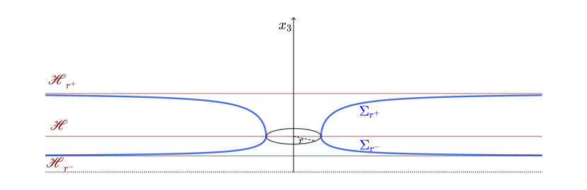
Figure 3. The profile curve of a translating catenoid $\varSigma_{r}$ in $\mathbb{H}^{3}$ bounded by (and asymptotic to) two horospheres $\mathscr{H}_{r^{-}}$ and $\mathscr{H}_{r^{+}}$. $\varSigma_{r}\setminus\mathscr{H}$ decomposes as two vertical graphs $\varSigma_{r}^{-}$ and $\varSigma_{r}^{+}$ over the complement of the Euclidean disk of radius $r$ centered at the rotation axis $x_{3}$ in the horosphere $\mathscr{H}$.

Theorem 3.9.

There exists a one-parameter family $\mathscr{C}:=\{\varSigma_{r}\mid r>0\}$ of noncongruent, properly embedded rotational annular translators in $\mathbb{H}^{3}$ (to be called translating catenoids). For each $r>0$, the surface $\varSigma_{r}\in\mathscr{C}$ satisfies:

• $\varSigma_{r}$ is contained in a slab determined by two horospheres $\mathscr{H}_{r^{-}}$ and $\mathscr{H}_{r^{+}}.$ In particular, the asymptotic boundary of $\varSigma_{r}$ is the point at infinity of the horosphere $\mathscr{H}$ at height $1$.

• $\varSigma_{r}$ is the union of two vertical graphs $\varSigma_{r}^{-}$ and $\varSigma_{r}^{+}$ over the complement of the Euclidean $r$-disk  $\mathcal{D}_{r}$ centered at the rotation axis in the horosphere $\mathscr{H}$.

• The graphs $\varSigma_{r}^{-}$ and $\varSigma_{r}^{+}$ lie in distinct connected components of  $\mathbb{H}^{3}-\mathscr{H}$ with common boundary the $r$-circle that bounds $\mathcal{D}_{r}$ in $\mathscr{H},$ being $\varSigma_{r}^{-}$ asymptotic to $\mathscr{H}_{r^{-}}$ and $\varSigma_{r}^{+}$ asymptotic to $\mathscr{H}_{r^{+}}.$

In addition, the limiting behaviour of $\varSigma_{r}$ is as follows:

• As $r\to 0,$ $\varSigma_{r}$ converges (on the $C^{2,\alpha}$-norm, on compact sets outside $(0,0,1)$) to a double copy of $\mathscr{H}.$

• As $r\to+\infty,$ the distance between $\varSigma_{r}$ and the $x_{3}$-axis becomes unbounded; in particular, $\varSigma_{r}$ escapes to infinity.

Proof.

Given $r>0,$ let $d_{r}:(1-\delta,1+\delta)\rightarrow(0,+\infty)$ be the local solution to the following initial value problem:

(20) $$\left\{\begin{array}[]{l}y^{\prime\prime}=\left(\frac{2y^{2}}{x^{2}}+1\right)\frac{1+(y^{\prime})^{2}}{y}\,,\\[4.30554pt] y(1)=r,\\[4.30554pt] y^{\prime}(1)=0.\end{array}\right.$$

By Lemma 3.8, the rotational horizontal graph $\varSigma_{r}$ determined by $d_{r}$ is a translator to MCF in $\mathbb{H}^{3}.$ Since $d_{r}$ is strictly convex, $x=1$ is a strict local minimum of $d_{r}$ and $\varSigma_{r}-\mathscr{H}$ is the union of two disjoint rotational vertical graphs $\varSigma_{r}^{-}$ and $\varSigma_{r}^{+}$ over an open set contained in $\mathscr{H}-\mathcal{D}_{r}.$ Let us index $\varSigma_{r}^{+}$ as being the component contained in the horoball $\{x_{3}>1\}$. Then, Lemma 3.6 applies to $\varSigma_{r}^{+}$, which corresponds to an increasing solution of (10) (i.e., one for which the initial condition $\lambda$ is positive). By Lemma 3.7, such a solution is defined in an interval $[x_{0},+\infty)$ and is bounded above. Therefore, $\varSigma_{r}^{+}$ can be continued indefinitely, being asymptotic to a horosphere $\mathscr{H}_{r^{+}}$ of $\mathbb{H}^{3}.$ In particular, $\varSigma_{r}^{+}$ is a graph over $\mathscr{H}-\mathcal{D}_{r}.$

Analogously, Lemmas 3.6 and 3.7 give that $\varSigma_{r}^{-}$ can be continued indefinitely and is asymptotic to a horosphere $\mathscr{H}_{r^{-}}$ of $\mathbb{H}^{3}.$ Since $\varSigma_{r}={\rm closure}(\varSigma_{r}^{-})\cup{\rm closure}(\varSigma_{r}^{+}),$ we have that $\varSigma_{r}$ is an annular properly embedded translator to MCF in $\mathbb{H}^{3}.$ This proves assertions (i)–(iii).

In the proof of assertions (iv) and (v), we will use the rotational symmetry of $\varSigma_{r}$ to work uniquely with the curves $G_{r}$, defined as the graphs of the solutions $d_{r}$ of (20), parameterized by

$$\alpha_{r}(s):=(0,d_{r}(s),s),\,\,\,s\in(r^{-},r^{+}).$$

Furthermore, let $G_{r}^{+}=\{\alpha_{r}(s)\mid s\in[1,r^{+})\}$ and $G_{r}^{-}=\{\alpha_{r}(s)\mid s\in(r^{-},1])\}$ be the respective intersections of $G_{r}$ with $\{x_{3}>1\}$ and $\{x_{3}<1\}$, and set $p_{r}=\alpha_{r}(1)=(0,r,1)$. We get directly from (20) that, with the induced Euclidean metric, the curvature of $G_{r}$ at $p_{r}$ is $k_{r}(1)=d_{r}^{\prime\prime}(1)=2r+1/r$, which gives (see Fig. 4):

(21) $${\lim_{r\to 0}k_{r}(1)=\lim_{r\to+\infty}k_{r}(1)=+\infty.}$$

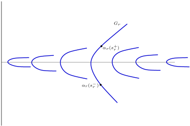
Figure 4. In the proof of Theorem 3.9, the curvature of the horizontal graph $G_{r}$ at the point of minimal Euclidean distance to the $x_{3}$-axis goes to infinity as $r$ goes to either $0$ or $+\infty.$

Now, set $r_{*}$ for either $0$ or $+\infty$. Then, equation (21), together with the fact that $d_{r}$ is strictly convex, increasing in $[1,r^{+})$ and decreasing in $(r^{-},1]$ allows us to choose points $p_{r}^{-}:=\alpha_{r}(s_{r}^{-})\in G_{r}^{-}$ and $p_{r}^{+}:=\alpha_{r}(s_{r}^{+})\in G_{r}^{+}$ satisfying (with respect to the Euclidean norm $\|\cdot\|$)

(22) $$\lim_{r\to r_{*}}\|p_{r}^{-}-p_{r}\|=\lim_{r\to r_{*}}\|p_{r}^{+}-p_{r}\|=0,$$

with unit tangent vectors so that

(23) $$\lim_{r\to r_{*}}\frac{\alpha_{r}^{\prime}(s_{r}^{+})}{\|\alpha_{r}^{\prime}(s_{r}^{+})\|}=-\lim_{r\to r_{*}}\frac{\alpha_{r}^{\prime}(s_{r}^{-})}{\|\alpha_{r}^{\prime}(s_{r}^{-})\|}=\partial_{x_{2}}.$$

Let $\ell_{r}^{+}$ and $\ell_{r}^{-}$ denote the tangent lines to $G_{r}$ at the points $p_{r}^{+}$ and $p_{r}^{-}$, respectively. Then, by convexity, it follows that $G_{r}$ lies in the region limited between $\ell_{r}^{+}$ and $\ell_{r}^{-}$ that contains $p_{r}$. Since (22) implies that

$$\lim_{r\to r_{*}}s_{r}^{-}=\lim_{r\to r_{*}}s_{r}^{+}=1,$$

it follows from (23) that both $\ell_{r}^{+}$ and $\ell_{r}^{-}$ converge to the horizontal line $\{(0,s,1)\mid s\in\mathbb{R}\}$, when $r\to r_{*}$, which immediately proves item (iv).

To prove item (v), we use that equidistant curves to the $x_{3}$-axis in the $x_{2}x_{3}$ halfplane are half-lines issuing from $(0,0,0)$; our next argument is to prove that there is no such curve that intersects $G_{r}$ for any $r>0$ arbitrarily large. Fix some $\lambda>0$ and consider the half-line $\ell=\{(0,x_{2},\lambda x_{2})\mid x_{2}>0\}$. Let $r_{1}>0$ be such that the slope of $\ell_{r}^{+}$ is less then $\lambda$ for all $r>r_{1}$ and let $r_{0}={\rm max}\{r_{1},1/\lambda\}$ (see Fig. 5). Then, if $r>r_{0}$, in the region $\{x_{2}\geq r\}$, the line $\ell$ is contained in $\{x_{3}>1\}$ and the line $\ell_{r}^{+}$ is below $\ell$. Since $G_{r}\subset\{x_{2}\geq r\}$, staying in one side of $\ell_{r}^{+}$, this yields $G_{r}\cap\ell=\emptyset$ for all $r>r_{0}$, as we wished to prove. ∎

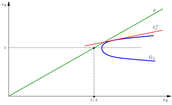
Figure 5. In the proof of Theorem 3.9, the equidistant halfline $\ell$ has no intersection with $G_{r}$ if $r>0$ is sufficiently large.

Let $\varSigma$ be a connected rotational translator in $\mathbb{H}^{3}$ with (possibly empty) boundary. If $\varSigma$ is not a horosphere, Lemmas 3.6 and 3.8, together with the uniqueness of solutions of ODE’s with given initial conditions, imply that the profile curve of $\varSigma$ coincides, up to its boundary, with the profile curve of some translating catenoid $\varSigma_{r}$ obtained in Theorem 3.9. Therefore, we have the following uniqueness result.

Theorem 3.10.

Any connected rotational translator of  $\mathbb{H}^{3}$ is either an open subset of a horosphere or of some translating catenoid.

3.2. Parabolic translators.

Having considered rotational translators in the previous section, we now look at translators which are invariant by a 1-parameter group of parabolic isometries of $\mathbb{H}^{3}$, i.e., isometries of $\mathbb{H}^{3}$ that fix parallel families of horospheres. Horizontal cylinders over curves on vertical totally geodesic planes of $\mathbb{H}^{3}$ (to be called parabolic cylinders) are the simplest examples of surfaces which are invariant by parabolic translations. When these generating curves are graphs on the whole of $\mathbb{R},$ such a surface can be parameterized by a map $X\colon\mathbb{R}^{2}\to\mathbb{R}_{+}^{3}$ defined by

$$X(u,v)=(u,v,\phi(v)),\,\,(u,v)\in\mathbb{R}^{2},$$

where $\phi$ is a smooth positive function on $\mathbb{R}.$ We shall call $\varSigma:=X(\mathbb{R}^{2})$ the parabolic cylinder determined by $\phi.$

Defining $\varrho(v):=(1+(\phi^{\prime}(v))^{2})^{-1/2},$ we have that

$$\bar{\eta}:=\varrho(0,-\phi^{\prime},1)$$

is a unit normal to $\varSigma$ with respect to the induced Euclidean metric of $\mathbb{R}_{+}^{3}.$ With this orientation, the Euclidean mean curvature $\mkern 1.5mu\overline{\mkern-1.5muH\mkern-1.5mu}\mkern 1.5mu$ of $\varSigma$ is

$$\mkern 1.5mu\overline{\mkern-1.5muH\mkern-1.5mu}\mkern 1.5mu=\frac{\varrho^{3}\phi^{\prime\prime}}{2}\,\cdot$$

From this last equality and (1), we have that the hyperbolic mean curvature $H$ of $\varSigma$ with respect to the orientation $\eta:=\phi\bar{\eta}$ is

$$H=\varrho\left(\frac{\varrho^{2}\phi\phi^{\prime\prime}}{2}+1\right).$$

Since $\langle\eta,X\rangle=\varrho(\phi-v\phi^{\prime})/\phi,$ we also have that the identity (4) for the parabolic cylinder $\varSigma=X(\mathbb{R}^{2})$ is equivalent to the following second order ODE:

$$\phi^{\prime\prime}=-\phi^{\prime}(1+(\phi^{\prime})^{2})\frac{2v}{\phi^{2}}\cdot$$

The above considerations yield

Lemma 3.11.

A parabolic cylinder determined by a smooth function $\phi$ is a translator to MCF in  $\mathbb{H}^{3}$ if and only if $\phi$ is a solution to the second order ODE:

(24) $$y^{\prime\prime}=-y^{\prime}(1+(y^{\prime})^{2})\frac{2x}{y^{2}}\cdot$$

The solutions of (24) are all increasing on $\mathbb{R}$ and their graphs are “S-shaped”, as attested by the following

Lemma 3.12.

Given $\lambda\geq 0,$ the initial value problem

(25) $$\left\{\begin{array}[]{l}y^{\prime\prime}=-y^{\prime}(1+(y^{\prime})^{2})\frac{2x}{y^{2}}\\[4.30554pt] y(0)=1\\[4.30554pt] y^{\prime}(0)=\lambda\end{array}\right.$$

has a unique smooth solution $\phi:\mathbb{R}\to\mathbb{R}$ which has the following properties:

• $\phi$ is constant if $\lambda=0.$

• $\phi$ is increasing, convex in $(-\infty,0),$ and concave in $(0,+\infty)$ if $\lambda>0.$

• $\phi$ is bounded above and below by positive constants.

Proof.

Assertion (i) is immediate. So, assume $\lambda>0.$ Proceeding as in the proof of Lemma 3.7, we get from the equality

(26) $$\phi^{\prime\prime}=-\phi^{\prime}(1+(\phi^{\prime})^{2})\frac{2x}{\phi^{2}}$$

that $\phi$ necessarily satisfies:

$$\phi^{\prime}(x)=\lambda\exp\left(\int_{0}^{x}F(t,\phi(t),\phi^{\prime}(t))\right)dt,$$

where $F$ is given by

$$F(x,y,z):=-\frac{2x}{y^{2}}(1+z^{2}).$$

Hence, $\phi$ is increasing. This, together with (26), implies that $\phi$ is defined in a maximal interval $I_{\rm max}:=(x_{\rm min},+\infty)$ with $-\infty\leq x_{\rm min}<0.$ It also follows from (26) that $\phi$ is convex in $(x_{\rm min},0),$ and concave in $(0,+\infty).$

Next, we prove that the solution $\phi$ is bounded above. Since $\phi$ is concave in $(0,+\infty),$ we have that $\lambda=\phi^{\prime}(0)>\phi^{\prime}(x)$ for all $x>0.$ Then, integration on both sides of this last inequality yields

$$\phi(x)\leq\lambda x+1\,\,\,\forall x\geq 0,$$

which implies that

(27) $$\lim_{x\to+\infty}\frac{x}{\phi(x)}\geq\lim_{x\to+\infty}\frac{x}{\lambda x+1}=\frac{1}{\lambda}>0.$$

Now, choose a small $\epsilon>0$ such that $C:=\lambda^{-1}-\epsilon$ is positive. It follows from (27) that, for a sufficiently large $x_{1}>0,$ one has $x/\phi(x)>C$ for all $x\geq x_{1},$ so that

$$\frac{2x}{\phi^{2}(x)}\geq\frac{2C^{2}}{x},\,\,\,\,\forall x\geq x_{1},$$

from which we obtain

(28) $$F(x,\phi(x),\phi^{\prime}(x))\leq-\frac{2C^{2}}{x},\,\,\,\forall x\geq x_{1}.$$

Now, for any given $x_{0}>0$, consider the following initial value problem:

(29) $$\left\{\begin{array}[]{l}y^{\prime\prime}=-y^{\prime}(1+(y^{\prime})^{2})\frac{2x}{y^{2}}\\[4.30554pt] y(x_{0})=\phi(x_{0})\\[4.30554pt] y^{\prime}(x_{0})=\phi^{\prime}(x_{0}).\end{array}\right.$$

By uniqueness, $\phi$ is a solution to (29), and once again we may write

(30) $$\phi^{\prime}(x)=\lambda_{0}\exp\left(\int_{x_{0}}^{x}F(t,\phi(t),\phi^{\prime}(t))\right)dt,\,\,\,\,\forall x\geq x_{0},$$

where $\lambda_{0}:=\phi^{\prime}(x_{0})>0.$ In particular, defining $\lambda_{1}=\phi^{\prime}(x_{1})$, we obtain

(31) $$\phi^{\prime}(x)=\lambda_{1}\exp\left(\int_{x_{1}}^{x}F(t,\phi(t),\phi^{\prime}(t))\right)dt,\,\,\,\,\forall x\geq x_{1}$$

and it follows from (28) and (31) that

$$\phi^{\prime}(x)\leq\lambda_{1}\left(\frac{x_{1}}{x}\right)^{2C^{2}},\,\,\,\forall x\geq x_{1},$$

so that $\phi^{\prime}(x)\to 0$ as $x\to+\infty.$ Therefore, we have

$$\lim_{x\to+\infty}\frac{x}{\phi(x)}=+\infty.$$

In particular, there exists $x_{2}\geq x_{1}$ such that the inequality

$$\frac{2x}{\phi^{2}(x)}\geq\frac{2}{x}$$

holds for all $x\geq x_{2},$ which gives that $F(x,\phi(x),\phi^{\prime}(x))<-2/x$ for all $x\geq x_{2}.$ Therefore, applying (30) for $x_{2}$,

$$\phi^{\prime}(x)=\lambda_{2}\exp\left(\int_{x_{2}}^{x}F(t,\phi(t),\phi^{\prime}(t))\right)dt,\,\,\,\lambda_{2}=\phi^{\prime}(x_{2})$$

and we may proceed just as in the proof of Lemma 3.7 to conclude that

$$\phi(x)-\phi(x_{2})\leq\lambda_{2}x_{2}^{2}\left(\frac{1}{x_{2}}-\frac{1}{x}\right)<\lambda_{2}x_{2},\quad\forall x\geq x_{2},$$

which implies that $\phi$ is bounded above.

Next, we show that $\phi$ is bounded below by a positive constant. With this purpose, assume by contradiction that

(32) $$\lim_{x\to x_{\rm min}}\phi(x)=0.$$

Reasoning as in the proof of item iii of Lemma 3.7, we obtain from this assumption that

(33) $$\lim_{x\to x_{\rm min}}\phi^{\prime\prime}(x)=+\infty,$$

which, in turn, implies that

(34) $$\lim_{x\to x_{\rm min}}\frac{\phi^{\prime}(x)}{\phi(x)}=+\infty.$$

Equality (33) gives that $\phi^{\prime\prime}$ is necessarily decreasing in a neighborhood of any sufficiently small $x\in(x_{\rm min},0).$ However, by computing $\phi^{\prime\prime\prime}$ from (26), we get

(35) $$\phi^{\prime\prime\prime}=-\phi^{\prime\prime}(1+(\phi^{\prime})^{2})\frac{2x}{\phi^{2}}-4(\phi^{\prime})^{2}\phi^{\prime\prime}\frac{x}{\phi^{2}}-\phi^{\prime}(1+(\phi^{\prime})^{2})\left(\frac{2}{\phi^{2}}-\frac{4x\phi^{\prime}}{\phi^{3}}\right).$$

Then, considering the equality $-\phi^{\prime}(1+(\phi^{\prime})^{2})=\phi^{2}\phi^{\prime\prime}/(2x),$ which we get from (26), and applying it to the last summand of (35), we obtain

$$\phi^{\prime\prime\prime}=\phi^{\prime\prime}\left[-\frac{2x}{\phi^{2}}(1+3(\phi^{\prime})^{2})+\frac{1}{x}-\frac{2\phi^{\prime}}{\phi}\right]=\phi^{\prime\prime}\left[-\frac{2x}{\phi^{2}}-2\frac{\phi^{\prime}}{\phi}\left(1+3x\frac{\phi^{\prime}}{\phi}\right)+\frac{1}{x}\right].$$

This last equality, together with equations (32)–(34), clearly yields

$$\lim_{x\to x_{\rm min}}\phi^{\prime\prime\prime}(x)=+\infty,$$

which contradicts (33). Therefore, we have

$$\lim_{x\to x_{\rm min}}\phi(x)>0,$$

from which we conclude that $\phi$ is bounded from below by a positive constant. In particular, we must have $x_{\min}=-\infty.$ This finishes the proof. ∎

Lemmas 3.11 and 3.12 immediately give the following result (see Fig. 6).

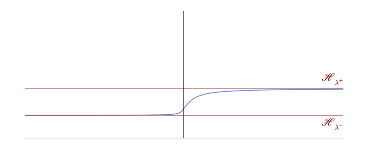
Figure 6. The profile curve of a hyperbolic grim reaper in $\mathbb{H}^{3}$ lying between two horospheres $\mathscr{H}_{\lambda^{-}}$ and $\mathscr{H}_{\lambda^{+}}$.

Theorem 3.13.

In hyperbolic space $\mathbb{H}^{3},$ there exists a one-parameter family

$$\mathscr{G}:=\{\varSigma_{\lambda}\mid\lambda\in[0,+\infty)\}$$

of noncongruent, complete translators (to be called grim reapers) which are horizontal parabolic cylinders generated by the solutions of (25). $\varSigma_{0}$ is the horosphere $\mathscr{H}\subset\mathbb{H}^{3}$ at height one, and for $\lambda>0,$ each $\varSigma_{\lambda}\in\mathscr{G}$ is an entire graph over $\mathbb{R}^{2}$ which is contained in a slab determined by two horospheres $\mathscr{H}_{\lambda^{-}}$ and $\mathscr{H}_{\lambda^{+}}.$ Furthermore, there exist open sets $\varSigma_{\lambda}^{-}$ and $\varSigma_{\lambda}^{+}$ of $\varSigma_{\lambda}$ such that $\varSigma_{\lambda}^{-}$ is asymptotic to $\mathscr{H}_{\lambda^{-}}$, $\varSigma_{\lambda}^{+}$ is asymptotic to $\mathscr{H}_{\lambda^{+}},$ and $\varSigma_{\lambda}={\rm closure}\,(\varSigma_{\lambda}^{-})\cup{\rm closure}\,(\varSigma_{\lambda}^{+}).$

If $\Gamma\subset\mathbb{R}^{2}$ is the graph of the function $t\in(-\pi/2,\pi/2)\mapsto-\log(\cos t)$, then the cylinder $\varSigma=\Gamma\times\mathbb{R}\subset\mathbb{R}^{3}$ is a translator to MCF contained in a slab $\mathcal{S}$ of $\mathbb{R}^{3}$, known as the grim reaper cylinder. This nomenclature is due to the fact that the curve $\Gamma$ provides a solution to the curve shortening flow, called the grim reaper, which is given by the translation of $\Gamma$ in $\mathbb{R}^{2}$ in the $\vec{e}_{2}$-direction. By the avoidance principle, such a solution “kills” any other solution in the region $(-\pi/2,\pi/2)\times\mathbb{R}$ (see [2, Chapter 2]). Similarly, two surfaces (one of them compact) in $\mathbb{R}^{3}$ moving under MCF which are initially disjoint remain so until one of them collapses. Hence, as $\varSigma$ translates under MCF, it “kills” all solutions to (2) in $\mathcal{S}$ with compact initial condition. An analogous process occurs in our case: any surface of the family $\mathscr{G}$ in Theorem 3.13 has this “killing” property. Indeed, by [7, Theorem 4], the avoidance principle applies to surfaces moving under MCF in $\mathbb{H}^{3}.$ For this reason, we named the elements of $\mathscr{G}$ grim reapers.

Remark 3.14.

The symmetry in (24) allows us to extend the family $\mathscr{G}$ in Theorem 3.13 for values $\lambda<0$ by simply defining $\psi(x)=\phi(-x)$ for a given solution $\phi$ to (25) with positive initial data for $\phi^{\prime}$. However, the translator generated by $\psi$ correspond to a rotation of $\pi$ around the $x_{3}$-axis of a grim reaper, being therefore congruent to it.

Remark 3.15.

At the completion of this manuscript, we became acquainted with the preprint [17], in which the authors consider solitons to MCF generated by conformal fields in $\mathbb{H}^{n}$, called conformal solitons. There, they obtained rotational and cylindrical conformal solitons whose initial conditions are named winglike catenoids and grim reaper cylinder, respectively. However, such solitons are not related to the ones considered here, since their generating fields are not Killing.

Analogously to the rotational case, the uniqueness of solutions of ODE’s with given initial conditions yields the following result.

Theorem 3.16.

Any connected translator in $\mathbb{H}^{3}$ which is a parabolic cylinder is, up to an ambient isometry (see Remark 3.14), an open subset of a grim reaper or of a totally geodesic plane containing the $x_{3}$-axis.

3.3. The tangency principle and applications.

A distinguished property of translators to MCF in $\mathbb{R}^{3}$ is that they are critical points of a weighted area functional and, therefore, they become minimal surfaces when changing the ambient metric in a suitable manner [14]. In particular, the tangency principle applies to them, which allows one to use translators as barriers (cf. [16]). On the other hand, it is unknown to us if translators to MCF in $\mathbb{H}^{3}$ can be made minimal in a similar fashion. Nevertheless, as we establish in the next result, the tangency principle holds for translators in $\mathbb{H}^{3}$.

Theorem 3.17 (tangency principle for translators).

Let $\varSigma_{1}$ and $\varSigma_{2}$ be two translators to MCF in $\mathbb{H}^{3}$ which are tangent at a point $p\in{\rm int}\,\varSigma_{1}\cap{\rm int}\,\varSigma_{2}.$ If $\varSigma_{1}$ lies on one side of $\varSigma_{2}$ in a neighborhood of $p$ in $\mathbb{H}^{3},$ then $\varSigma_{1}$ and $\varSigma_{2}$ coincide in a neighborhood of $p$ in $\varSigma_{1}\cap\varSigma_{2}.$ Moreover, if $\varSigma_{1}$ and $\varSigma_{2}$ are both complete and connected, then $\varSigma_{1}=\varSigma_{2}.$

Proof.

Let $\varSigma_{1}$ and $\varSigma_{2}$ be two translators to MCF in $\mathbb{H}^{3}$, tangent at a point $p\in\varSigma_{1}\cap\varSigma_{2}$, and such that $\varSigma_{1}$ stays locally on one side of $\varSigma_{2}$. If $T_{p}\varSigma_{1}$ is not vertical, there exists a domain $\Omega\subset\mathbb{R}^{2}$ and positive functions $u_{1},\,u_{2}\colon\Omega\to\mathbb{R}$ such that neighborhoods $U_{1}\subset\varSigma_{1}$ and $U_{2}\subset\varSigma_{2}$ containing $p$ are respectively parameterized by

$$U_{1}=\{(x,y,u_{1}(x,y))\mid(x,y)\in\Omega\},\quad U_{2}=\{(x,y,u_{2}(x,y))\mid(x,y)\in\Omega\}.$$

Furthermore, after reindexing we may assume that $u_{1}\geq u_{2}$ in $\Omega$.

Let $\varSigma_{1}$ and $\varSigma_{2}$ be oriented with respect to vector fields $\eta_{1}$ and $\eta_{2}$ so that $\eta_{1}(p)=\eta_{2}(p)$ points upwards. Thus, if $Q$ is the quasilinear elliptic operator

(36) $$Q(u)=u_{xx}(1+u_{y}^{2})+u_{yy}(1+u_{x}^{2})-2u_{xy}u_{x}u_{y},$$

it follows from (1) that the mean curvature functions $H_{1},\,H_{2}$ of $U_{1}$ and $U_{2}$ satisfy

$$H_{i}=u_{i}\frac{Q(u_{i})}{2(1+(u_{i})_{x}^{2}+(u_{i})_{y}^{2})^{\frac{3}{2}}}+\frac{1}{(1+(u_{i})_{x}^{2}+(u_{i})_{y}^{2})^{\frac{1}{2}}},\quad i\in\{1,2\}.$$

Then, after setting $B(x,y,u,Du)=2(1+u_{x}^{2}+u_{y}^{2})(xu_{x}+yu_{y})$, where $Du$ denotes the (Euclidean) gradient of $u$, it follows from (4) that

(37) $$(u_{i})^{2}Q(u_{i})+B(x,y,u_{i},Du_{i})=0,\quad i\in\{1,2\}.$$

But the operator $u^{2}Q(u)+B(x,y,u,Du)$ in (37) satisfies the hypothesis of the tangency principle for quasilinear operators [19, Theorem 2.2.2], thus $u_{1}=u_{2}$, which implies $U_{1}=U_{2}$.

The case where $T_{p}\varSigma_{1}$ is vertical can be treated analogously: after a rotation about the $x_{3}$-axis (which preserves the property of being a translator to MCF), locally, both $\varSigma_{1}$ and $\varSigma_{2}$ can be parameterized as horizontal graphs

$$\{(x,u_{1}(x,z),z)\mid(x,z)\in\widehat{\Omega}\}\,\,\,\text{and}\,\,\,\{(x,u_{2}(x,z),z)\mid(x,z)\in\widehat{\Omega}\}$$

for some domain $\widehat{\Omega}\subset\mathbb{R}^{2}_{+}$, and both $u_{1},\,u_{2}$ satisfy

$$z^{2}Q(u)+\widehat{B}(x,z,u,Du)=0$$

for $\widehat{B}(x,z,u,Du)=2(xu_{x}-u)(1+u_{x}^{2}+u_{z}^{2})$ and $Q$ as in (36). Once again, we obtain from [19, Theorem 2.22] that $\varSigma_{1}$ and $\varSigma_{2}$ coincide in a neighborhood of $p$.

At this point, we have shown that if $\varSigma_{1}$ and $\varSigma_{2}$ are tangent at a point $p$, they must coincide in neighborhoods which are either horizontal or vertical graphs for $\varSigma_{1}$ and $\varSigma_{2}$. The proof for the case where $\varSigma_{1}$ and $\varSigma_{2}$ are complete and connected now follows from covering $\varSigma_{1}$ and $\varSigma_{2}$ with such (overlapping) neighborhoods. ∎

Remark 3.18.

Theorem 3.17 contrasts with the tangency principle for the constant mean curvature case (see, for instance, [15, Theorem 3.2.4]): two distinct geodesic spheres in $\mathbb{R}^{3}$ with the same mean curvature can be tangent to each other without violating the tangency principle. In the setting of translators, the tangency principle does not require any assumptions on the orientation of $\varSigma_{1}$ and $\varSigma_{2}$ because, from (4), if $\varSigma_{1}$ and $\varSigma_{2}$ are translators to MCF which are tangent at a point $p$, then necessarily their mean curvature vectors $\mathbf{H}_{1}$ and $\mathbf{H}_{2}$ must agree at $p$, which defines a coinciding, standard (local) orientation for both $\varSigma_{1}$ and $\varSigma_{2}$.

On the remainder of the section we will apply the tangency principle to establish some classification results concerning translators in $\mathbb{H}^{3}$. First, we show that properly immersed translators in $\mathbb{H}^{3}$ are never cylindrically bounded, and next we prove that any horoconvex translator which is complete or transversal to the $x_{3}$-axis is necessarily an open set of a horizontal horosphere.

Recall that a circular cone in $\mathbb{R}_{+}^{3}:=\mathbb{R}^{2}\times(0,+\infty)$ with vertex at $p\in\mathbb{R}^{2}$ and axis $\gamma_{p}:=\{p\}\times(0,+\infty)$ constitutes a cylinder $\mathscr{C}$ in $\mathbb{H}^{3},$ that is, the set of points of $\mathbb{H}^{3}$ at a fixed distance to the vertical geodesic $\gamma_{p}.$ The convex side of $\mathscr{C}$ is the component of $\mathbb{H}^{3}-\mathscr{C}$ which contains $\gamma_{p}.$

Theorem 3.19.

There is no properly immersed translator to MCF in $\mathbb{H}^{3}$ which is contained in the convex side of a cylinder with vertex at $p=(0,0).$ In particular, there is no closed (i.e., compact without boundary) translator to MCF in $\mathbb{H}^{3}$.

Proof.

Suppose, by contradiction, that there exists a properly immersed translator $\varSigma$ to MCF in $\mathbb{H}^{3}$ which is contained in the convex side $\Omega$ of a cylinder $\mathcal{C}$ with vertex at $p=(0,0).$ Clearly, the property of being a translator is invariant by the translations $\Gamma_{t}(p):=e^{t}p,\,t\in\mathbb{R}.$ Therefore, we can assume without loss of generality that $\varSigma$ intersects the horosphere $\mathscr{H}$ of height $1.$

Under the above conditions, we have from item (v) of Theorem 3.9 that there exists $R>0$ such that, for any $r>R,$ the translating catenoid $\varSigma_{r}$ of the family $\mathscr{C}$ is disjoint from $\mathcal{C},$ and so from $\varSigma.$ On the other hand, for a sufficiently small $r>0,$ $\varSigma_{r}$ and $\varSigma$ have nonempty intersection. Taking into account the asymptotic behavior of $\varSigma_{r}$, together with the hypothesis that $\varSigma$ is contained in $\Omega,$, as $r$ decreases from $R$ to zero, a standard argument shows that there will be a first value $r_{*}$ such that $\varSigma_{r_{*}}$ is the element of $\mathscr{C}$ that first establishes a contact with $\varSigma$ at a point $p\in\varSigma\cap\varSigma_{r_{*}}$, as in Figure 7. Then, $\varSigma$ and $\varSigma_{r_{*}}$ are tangent at $p$ with $\varSigma$ on one side of $\varSigma_{r}$, and the tangency principle (Theorem 3.17) applies to show that $\varSigma=\varSigma_{r_{*}},$ which is a contradiction, since $\varSigma$ is contained in $\Omega$ and $\varSigma_{r_{*}}$ is not. ∎

Figure 7. In the proof of Theorem 3.19, there exists a smallest $r_{*}>0$ such that $\varSigma_{r_{*}}$ intersects $\varSigma$ tangentially, with $\varSigma$ in one of the two regions of $\mathbb{H}^{3}$ defined by $\varSigma_{r_{*}}$.

An oriented surface $\varSigma$ of $\mathbb{H}^{3}$ is called horoconvex if its principal curvatures $k_{1},k_{2}$ satisfy $k_{i}\geq 1$, $i=1,2.$ It is well known that every point $p$ of a horoconvex surface $\varSigma\subset\mathbb{H}^{3}$ is locally supported by a horosphere $\mathcal{H}$, meaning that $\mathcal{H}$ is tangent to $\varSigma$ at $p$, and there exists a neighborhood of $p$ in $\varSigma$ which lies in the horoball bounded by $\mathcal{H}$ (see, e.g., [4, Lemma 1]). Since the tangency principle immediately implies that no translator can attain a local maximum or local minimum for its height function, we obtain that any horoconvex translator whose tangent plane is horizontal at one of its points is necessarily an open set of a horizontal horosphere. With these considerations, we are in position to establish the following uniqueness result.

Theorem 3.20.

Let $\varSigma$ be a horoconvex translator in $\mathbb{H}^{3}$ and assume that one of the following occurs:

1. $\varSigma$ is complete.

2. $\varSigma$ intersects the $x_{3}$-axis transversely.

Then, $\varSigma$ is an open set of a horizontal horosphere.

Proof.

Let $\varSigma$ be as stated. By the comments above, in order to prove that $\varSigma$ is an open set of a horizontal horosphere, it suffices to show that the tangent plane of $\varSigma$ is horizontal at one of its points.

First, assume that item i) holds, so Theorem 3.19 implies that $\varSigma$ is noncompact. The main results in [4] show that horospheres are the unique complete and noncompact horoconvex surfaces of $\mathbb{H}^{3}$, so $\varSigma$ is a horosphere. In particular, there is a point $p\in\varSigma$ where $T_{p}\varSigma$ is horizontal, so $\varSigma$ is a horizontal horosphere.

Assume now that $\varSigma$ intersects the $x_{3}$-axis transversally at a point. Then, there is an open neighborhood $U$ of $\varSigma$ which is a graph of a smooth function $u$ over an open ball $\Omega\subset\mathbb{R}^{2}$ centered at the origin $(0,0)$. Since $\varSigma$ is a translator, $u$ satisfies (see the proof of Theorem 3.17),

(38) $$u^{2}Q(u)+B(x,y,u,Du)=0,$$

where $Q$ is defined by (36) and $B(x,y,u,Du)=2(1+u_{x}^{2}+u_{y}^{2})(xu_{x}+yu_{y})$. In addition, it follows from the horoconvexity of $\varSigma$ that its mean curvature $\mkern 1.5mu\overline{\mkern-1.5muH\mkern-1.5mu}\mkern 1.5mu$ with respect to the induced Euclidean metric cannot change sign, being either everywhere nonpositive or everywhere nonnegative, which, when orienting $U$ with respect to the upwards pointing normal, correspond to the respective cases $Q(u)\geq 0$ or $Q(u)\leq 0$.

First, assume that $Q(u)\geq 0$. Then, it follows from (38) that

(39) $$xu_{x}(x,y)+yu_{y}(x,y)\leq 0\,\,\,\forall(x,y)\in\Omega.$$

Let $\theta\in[0,\pi]$ be given and consider $u_{\theta}(t)=u(t\cos(\theta),t\sin(\theta))$, the restriction of $u$ to the line through the origin $L_{\theta}=\{(t\cos(\theta),t\sin(\theta))\mid t\in\mathbb{R}\}\cap\Omega$. Then, (39) implies that

$$tu_{\theta}^{\prime}(t)=t\cos(\theta)u_{x}(t\cos(\theta),t\sin(\theta))+t\sin(\theta)u_{y}(t\cos(\theta),t\sin(\theta))\leq 0.$$

In particular, $u_{\theta}^{\prime}(t)\geq 0$ when $t<0$ and $u_{\theta}^{\prime}(t)\leq 0$ when $t>0$, therefore $t=0$ is a point where $u_{\theta}$ assumes a local maximal value. Since $\theta$ is any given value in the compact set $[0,\pi]$, this implies that the tangent plane of $\varSigma$ at $p=(0,0,u(0,0))$ is horizontal, as we wished to prove.

The case when $Q(u)\leq 0$ (i.e., when the mean curvature vector of $\varSigma$ points downwards) can be treated analogously. ∎

Remark 3.21.

The horoconvexity hypothesis in Theorem 3.20 is necessary to the conclusion, since translating catenoids and grim reapers are complete, and any grim reaper is transversal to the $x_{3}$-axis. Furthermore, as we proved in Theorem 3.9-(iv), horizontal horospheres are limits of hyperbolic translating catenoids, so that they constitute the analogues of the bowl soliton of $\mathbb{R}^{3}$ (cf. [6]). From this point of view, Theorem 3.20 relates to certain uniqueness results for the bowl soliton, such as the celebrated theorem by Wang [21], which asserts that the bowl soliton is the only convex entire translator of $\mathbb{R}^{3}$.

4. Rotators to MCF in $\mathbb{H}^{3}$

Let us consider now the one-parameter group $\mathcal{G}\subset{\rm Iso}(\mathbb{H}^{3})$ of rotations $\Gamma_{t}$ of $\mathbb{H}^{3}=(\mathbb{R}_{+}^{3},ds^{2})$ about the $x_{3}$-axis. Considering the decomposition $\mathbb{R}_{+}^{3}=\mathbb{R}^{2}\times(0,+\infty),$ we have that

$$\Gamma_{t}=\left[\begin{array}[]{cc}e^{tJ}&\\ &1\end{array}\right],\quad J=\begin{bmatrix}0&-1\\ 1&\phantom{-}0\end{bmatrix}.$$

In this setting, an initial condition of a $\mathcal{G}$-soliton will be called a rotating soliton or simply a rotator. The (horizontal) Killing field associated to $\mathcal{G}$ is $\xi(p)=J\pi(p),$ $p\in\mathbb{H}^{3},$ where $\pi$ denotes the projection over $\{(0,0,1)\}^{\perp}\subset\mathbb{R}^{3}$, i.e., $\pi(x_{1},x_{2},x_{3})=x_{1}\partial_{x_{1}}+x_{2}\partial_{x_{2}}$. Hence, a surface $\varSigma$ of hyperbolic space $\mathbb{H}^{3}$ is a rotator to MCF if and only if

(40) $$H(p)=\langle J\pi(p),\eta(p)\rangle\,\,\,\forall p\in\varSigma.$$

Clearly, a minimal surface of $\mathbb{H}^{3}$ is a (stationary) rotator if and only if it is invariant by rotations about the $x_{3}$-axis. These minimal surfaces were classified in [5], and they include, of course, the one-parameter family of totally geodesic planes which intersect the $x_{3}$-axis orthogonally, as well as the hyperbolic catenoid obtained by Mori [18]. On the other hand, it is clear that no horosphere is a rotator in $\mathbb{H}^{3}$. These facts, together with the considerations of Remark 3.5, yield

Theorem 4.1.

The only rotators of constant mean curvature in $\mathbb{H}^{3}$ are the minimal surfaces of revolution with axis $\{(0,0)\}\times(0,+\infty).$

We shall seek for rotators in $\mathbb{H}^{3}$ in the class of helicoidal surfaces, which are described as follows. Choose a smooth curve with trace contained in the horosphere $\mathscr{H}:=\mathbb{R}^{2}\times\{1\}$ of height $1:$

$$s\in\mathbb{R}\mapsto(\alpha(s),1)\in\mathscr{H},$$

where $\alpha\colon\mathbb{R}\rightarrow\mathbb{R}^{2}$ is a regular curve parameterized by arc length. Given a constant $h>0,$ we call a parameterized surface $\varSigma=X(\mathbb{R}^{2})\subset\mathbb{H}^{3}$ a helicoidal surface generated by $\alpha$ with pitch $h$ if the parameterization $X:\mathbb{R}^{2}\rightarrow\mathbb{H}^{3}$ writes as

(41) $$X(u,v)=e^{hv}(e^{vJ}\alpha(u),1),\,\,\,(u,v)\in\mathbb{R}^{2}.$$

Considering a parameterization of $\alpha$ by arc length, $\alpha(s)=(u(s),v(s),0),\,s\in\mathbb{R},$ and writing

$$T(s)=u^{\prime}(s)\partial_{x}+v^{\prime}(s)\partial_{y},\quad N(s)=-v^{\prime}(s)\partial_{x}+u^{\prime}(s)\partial_{y},$$

the curvature of $\alpha$ is given by

$${k(s)=\langle\alpha^{\prime\prime}(s),N(s)\rangle_{e}=-u^{\prime\prime}(s)v^{\prime}(s)+v^{\prime\prime}(s)u^{\prime}(s),}$$

where $\langle\,,\,\rangle_{e}$ stands for the Euclidean metric of $\mathbb{R}^{2}.$ Furthermore, by the well known Frenet-Serret equations, one has

$${T^{\prime}=kN,\quad N^{\prime}=-kT.}$$

In this setting, if we define the functions

(42) $$\uptau:=\langle\alpha,T\rangle_{{e}}\quad\text{and}\quad\mu:=\langle\alpha,N\rangle_{{e}},$$

we get from a direct computation that

(43) $$\mkern 1.5mu\overline{\mkern-1.5mu\eta\mkern-1.5mu}\mkern 1.5mu=\varrho(e^{vJ}N,-(\uptau+h\mu)/h),\,\,\,\varrho:=h(h^{2}+(\uptau+h\mu)^{2})^{-1/2},$$

is an Euclidean unit normal to the helicoidal surface $\varSigma,$ and that its Euclidean mean curvature in this orientation is

$$\mkern 1.5mu\overline{\mkern-1.5muH\mkern-1.5mu}\mkern 1.5mu=e^{-hv}\varrho\frac{k((h^{2}+1)r^{2}+h^{2})-(h\uptau-\mu)}{2(h^{2}+(\uptau+h\mu)^{2})},$$

where $r^{2}:=\uptau^{2}+\mu^{2}.$ From this equality and (1), we have that the hyperbolic mean curvature $H$ of $\varSigma$ is

(44) $$H=\frac{\varrho}{h}\left(h\frac{k((h^{2}+1)r^{2}+h^{2})-(h\uptau-\mu)}{2(h^{2}+(\uptau+h\mu)^{2})}-(\uptau+h\mu)\right).$$

These considerations yield the following existence result, which brings [10, Theorem 3.1] to $\mathbb{H}^{3}$.

Theorem 4.2.

For any smooth function $\Psi\colon\mathbb{R}^{2}\rightarrow\mathbb{R}$ and any constant $h>0,$ there exists a one-parameter family of complete helicoidal surfaces of pitch $h$ in $\mathbb{H}^{3}$ each of them with mean curvature function $H$ satisfying

$$H(X(u,v))=\Psi(\uptau(u),\mu(u)),$$

where $X$ is the parameterization given in (41) and $\uptau$ and $\mu$ are as in (42).

Proof.

Considering equality (44) for the given function $H=H(\uptau,\mu)$ and solving for $k,$ we have that $k=k(\uptau,\mu)$ is a smooth function of $(\uptau,\mu)\in\mathbb{R}^{2}.$ However, by [10, Lemma 3.2], there exists a one-parameter family of plane curves $\alpha:\mathbb{R}\rightarrow\mathbb{R}^{2},$ each of them with curvature $k.$ Therefore, for such an $\alpha,$ and for a given $h>0,$ the helicoidal surface of $\mathbb{H}^{3}$ with pitch $h$ whose generating curve is $\alpha$ has mean curvature function $H=H(\uptau,\mu),$ as we wished to prove. ∎

Now, we verify the conditions under which a helicoidal surface $\varSigma=X(\mathbb{R}^{2})$ of $\mathbb{H}^{3}$ is a rotator to MCF. By (41)–(43),

$$\langle J\pi(X),\eta(X)\rangle = {\langle J(e^{hv}e^{vJ}\alpha),e^{hv}\mkern 1.5mu\overline{\mkern-1.5mu\eta\mkern-1.5mu}\mkern 1.5mu(X)\rangle}={\langle Je^{vJ}\alpha,\mkern 1.5mu\overline{\mkern-1.5mu\eta\mkern-1.5mu}\mkern 1.5mu(X)\rangle_{e}}$$

$$= {\langle e^{vJ}J\alpha,\varrho e^{vJ}N\rangle_{e}=\varrho\langle J\alpha,N\rangle_{e}}$$

$$= {-\varrho\langle\alpha,JN\rangle_{e}=\varrho\langle\alpha,T\rangle_{e}}$$

$$= \varrho\uptau,$$

which, together with (40), implies the following result.

Lemma 4.3.

A helicoidal surface $\varSigma=X(\mathbb{R}^{2})$ of pitch $h>0$ parameterized as in (41) is a rotator to MCF in $\mathbb{H}^{3}$ if and only if its mean curvature function $H=H(\uptau,\mu)$ satisfies

(45) $$H=\frac{h\uptau}{\sqrt{h^{2}+(h\mu+\uptau)^{2}}}.$$

In what follows, we prove the main result of this section, which provides the existence of complete rotators in $\mathbb{H}^{3}$ by means of helicoidal surfaces, and completely describe the topology of the corresponding generating curves (see Figure 8).

Figure 8. The generating curve of a helicoidal rotator in $\mathbb{H}^{3}$.

Theorem 4.4.

For any $h>0,$ there exists a one-parameter family of complete rotators to MCF in $\mathbb{H}^{3}$ whose elements are all helicoidal surfaces of pitch $h.$ For each such surface, the trace of the generating curve $\alpha\colon\mathbb{R}\to\mathbb{R}^{2}$ consists of two unbounded properly embedded arms centered at the point of $\alpha$ which is closest to the origin $o\in\mathbb{R}^{2},$ with each arm spiraling around $o.$

Proof.

The existence part of the statement follows directly from Lemma 4.3 and Theorem 4.2. So, it remains to prove that the generating curve $\alpha$ of any such helicoidal surface has the asserted geometric properties.

Keeping the above notation, we first observe that, from equalities (44) and (45), the curvature $k$ of $\alpha$ satisfies:

(46) $$k=\frac{2(h^{2}+(\uptau+h\mu)^{2})((h+1)\uptau+h\mu)+h(h\uptau-\mu)}{h((h^{2}+1)r^{2}+h^{2})}\cdot$$

Also, from (42) and the Frenet-Serret equations, one has

(47) $$\uptau^{\prime}=1+k\mu\quad\text{and}\quad\mu^{\prime}=-k\uptau,$$

which, together with (46), yields the ODE system (see Fig. 9)

(48) $$\left\{\begin{array}[]{ccl}\uptau^{\prime}&=&\displaystyle 1+\frac{2(h^{2}+(\uptau+h\mu)^{2})((h+1)\uptau\mu+h\mu^{2})+h^{2}\uptau\mu-h\mu^{2}}{h((h^{2}+1)r^{2}+h^{2})},\\[12.91663pt] \mu^{\prime}&=&\displaystyle-\frac{2(h^{2}+(\uptau+h\mu)^{2})((h+1)\uptau^{2}+h\uptau\mu)+h^{2}\uptau^{2}-h\uptau\mu}{h((h^{2}+1)r^{2}+h^{2})}\cdot\end{array}\right.$$

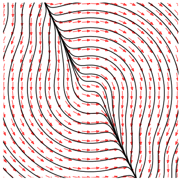
Figure 9. Phase portrait of system (48) for $h=1.$

Now, we establish the properties of $\alpha=\uptau T+\mu N$ through the following claims.

Claim 4.5.

The ODE system (48) has no constant solutions, and all solutions are defined on $\mathbb{R}.$

Proof of Claim 4.5.

Assume, by contradiction, that there exists a constant solution $\psi(s)=(\uptau_{0},\mu_{0}),\,s\in\mathbb{R}.$ Since $\uptau^{\prime}=\mu^{\prime}=0,$ we have from (47) that $k_{0}:=k(\uptau_{0},\mu_{0})$ satisfies $k_{0}\mu_{0}=-1$ and $k_{0}\uptau_{0}=0,$ which yields $\uptau_{0}=0$ and $\mu_{0}\neq 0.$ However, from the first equation in (48), one has

$$\uptau^{\prime}=1+\frac{2h(1+\mu_{0}^{2})\mu_{0}^{2}-\mu_{0}^{2}}{(h^{2}+1)\mu_{0}^{2}+h^{2}}=\frac{h^{2}(\mu_{0}^{2}+1)+2h(1+\mu_{0}^{2})\mu_{0}^{2}}{(h^{2}+1)\mu_{0}^{2}+h^{2}}>0,$$

which is a contradiction. Therefore, (48) has no constant solutions. From this fact, and since $k=k(\uptau,\mu)$ is defined on $\mathbb{R}^{2},$ we conclude that any solution of (48) is defined on $\mathbb{R}.$ ∎

Claim 4.6.

Suppose that any integral curve $\psi(s):=(\uptau(s),\mu(s))$ of (48) satisfies that the limit $\lim_{s\to+\infty}\uptau(s)$ (resp. $\lim_{s\to+\infty}\mu(s)$) exists. Then, $\lim_{s\to-\infty}\uptau(s)$ (resp. $\lim_{s\to-\infty}\mu(s)$) also exists. Furthermore, if there exists some $L\in[-\infty,+\infty]$ with the property that for any integral curve

$$\lim_{s\to+\infty}\uptau(s)=L\,\,\,(\text{resp.}\,\,\lim_{s\to+\infty}\mu(s)=L),$$

then it also holds that any integral curve satisfies

$$\lim_{s\to-\infty}\uptau(s)=-L\,\,\,(\text{resp.}\,\,\lim_{s\to-\infty}\mu(s)=-L).$$

Proof of Claim 4.6.

Let $\psi(s):=(\uptau(s),\mu(s))$ be an integral curve of the system (48). Then, it is easily checked that $\mkern 1.5mu\overline{\mkern-1.5mu\psi\mkern-1.5mu}\mkern 1.5mu(s):=-\psi(-s)$ is also an integral curve of that system. Setting $\mkern 1.5mu\overline{\mkern-1.5mu\psi\mkern-1.5mu}\mkern 1.5mu=(\mkern 1.5mu\overline{\mkern-1.5mu\uptau\mkern-1.5mu}\mkern 1.5mu,\mkern 1.5mu\overline{\mkern-1.5mu\mu\mkern-1.5mu}\mkern 1.5mu),$ we have that $\mkern 1.5mu\overline{\mkern-1.5mu\uptau\mkern-1.5mu}\mkern 1.5mu(s)=-\uptau(-s)$ and $\mkern 1.5mu\overline{\mkern-1.5mu\mu\mkern-1.5mu}\mkern 1.5mu(s)=-\mu(-s).$ By hypothesis, $\lim_{s\to+\infty}\mkern 1.5mu\overline{\mkern-1.5mu\uptau\mkern-1.5mu}\mkern 1.5mu(s)$ exists and the first part of the claim follows from observing that $\lim_{s\to-\infty}\mu(s)=-\lim_{s\to+\infty}\mkern 1.5mu\overline{\mkern-1.5mu\mu\mkern-1.5mu}\mkern 1.5mu(s)$. The remainder of the proof is argued analogously and will be omitted. ∎

Claim 4.7.

The function $\uptau$ has precisely one zero $s_{0}$ and $\uptau$ is negative in $(-\infty,s_{0})$ and positive in $(s_{0},+\infty).$ As a consequence, the function $r^{2}=\uptau^{2}+\mu^{2}$ has a global minimum and satisfies $\lim_{s\rightarrow\pm\infty}r^{2}=+\infty.$

Proof of Claim 4.7.

First, observe that the equalities (47) yield

$$(r^{2})^{\prime}=2(\uptau\uptau^{\prime}+\mu\mu^{\prime})=2(\uptau(1+k\mu)+\mu(-k\uptau))=2\uptau,$$

which implies that the zeroes of $\uptau$ are the critical points of $r^{2}$. Also, as seen in the first part of the proof of Claim 4.5, if $\uptau(s_{0})=0$ for some $s_{0},$ then $\uptau^{\prime}(s_{0})>0,$ which gives that $\uptau$ has at most one zero $s_{0},$ in which case $\uptau$ is negative in $(-\infty,s_{0}),$ and positive in $(s_{0},+\infty).$

Next, we argue by contradiction and assume that $\uptau$ has no zeroes. We will also assume that $\uptau>0$ on $\mathbb{R},$ since the complementary case $\uptau<0$ can be treated analogously. Under this assumption, the function $r^{2}$ is strictly increasing. So, there exists $\delta\geq 0$ such that

$$\lim_{s\to-\infty}r^{2}(s)=\delta.$$

In particular, since $\uptau=\frac{(r^{2})^{\prime}}{2}$, we also have that

(49) $$\lim_{s\to-\infty}\uptau(s)=0,$$

which implies that $\mu^{2}\rightarrow\delta$ as $s\rightarrow-\infty.$ However, the first equality in (48) yields $\lim_{s\rightarrow-\infty}\uptau^{\prime}(s)>0,$ which contradicts (49), proving that $\uptau$ has exactly one zero and that $r^{2}$ has only one critical point. Consequently, both the limits of $r^{2}$ as $s\rightarrow\pm\infty$ exist in $[0,+\infty]$.

To finish the proof of the claim, just note that if either $\lim_{s\to-\infty}r^{2}=\delta$ or $\lim_{s\to+\infty}r^{2}=\delta$ for some $\delta>0,$ the same arguments as before lead to a contradiction, thus $\lim_{s\to\pm\infty}r^{2}(s)=+\infty$. ∎

Claim 4.8.

The limits of $\uptau$ and $\mu$ as $s\rightarrow\pm\infty$ exist (possibly being infinite).

Proof of Claim 4.8.

First, we show that $k$ has at most one zero in $\mathbb{R}.$ Assume that $k(s_{0})=0$ for some $s_{0}\in\mathbb{R}.$ We have from (46) that, at $s_{0},$

(50) $$2(h^{2}+(\uptau+h\mu)^{2})((h+1)\uptau+h\mu)+h(h\uptau-\mu)=0.$$

Also, by (47), $\uptau^{\prime}(s_{0})=1$ and $\mu^{\prime}(s_{0})=0.$ This, together with (50), gives that, at $s_{0},$

(51) $$k^{\prime}=\frac{2(h+1)(h^{2}+(\uptau+h\mu)^{2})+4((h+1)\uptau+h\mu)(\uptau+h\mu)+h^{2}}{h((h^{2}+1)r^{2}+h^{2})}\cdot$$

If $\uptau(s_{0})\mu(s_{0})\geq 0,$ we have from (51) that $k^{\prime}(s_{0})>0.$ Assume then $\uptau(s_{0})\mu(s_{0})<0$ and notice that, by (50), one has

(52) $${\rm sign}((h+1)\uptau(s_{0})+h\mu(s_{0}))={\rm sign}(\mu(s_{0})-h\uptau(s_{0})).$$

If $\uptau(s_{0})<0<\mu(s_{0}),$ then both signs in (52) are positive. In addition,

$$\uptau(s_{0})+h\mu(s_{0})=(h+1)\uptau(s_{0})+h\mu(s_{0})-h\uptau(s_{0})>0,$$

and then (51) yields $k^{\prime}(s_{0})>0.$ Analogously, $\mu(s_{0})<0<\uptau(s_{0})$ implies $k^{\prime}(s_{0})>0.$

It follows from the above that $k$ has at most one zero $s_{0}\in\mathbb{R}$ and, if so, $k$ is negative in $(-\infty,s_{0})$ and positive in $(s_{0},+\infty).$ Since, by Claim 4.7, $\uptau$ has exactly one zero, we have that $\mu^{\prime}=-k\uptau$ has at most two zeros, which implies that $\mu$ has at most two critical points. In particular, the limits $\lim_{s\to\pm\infty}\mu(s)$ exist.

To finish the proof of the claim, let us assume, by contradiction, that the limit of $\uptau$ as $s\rightarrow+\infty$ does not exist. In this case, for some $\uptau_{0}>0,$ there exists a strictly increasing sequence $(s_{n})_{n\in\mathbb{N}}$ diverging to $+\infty$ and such that (see Fig. 10)

$$\uptau(s_{n})=\uptau_{0}\quad\text{and}\quad\uptau^{\prime}(s_{n})\uptau^{\prime}(s_{n+1})<0\quad\forall n\in\mathbb{N}.$$

Figure 10. Graph of $\uptau.$

Claim 4.7 implies that $\lim r^{2}(s_{n})=+\infty$, then we must have $\lim\mu^{2}(s_{n})=+\infty$. In this case, our previous arguments show that either $\lim\mu(s_{n})=+\infty$ or $\lim\mu(s_{n})=-\infty$. In any case, we have from (46) that

$$\lim_{n\to+\infty}(k(s_{n})\mu(s_{n}))=\lim_{n\to+\infty}\frac{2h^{3}\mu(s_{n})^{4}}{h(h^{2}+1)\mu(s_{n})^{2}}=+\infty.$$

In particular, for any sufficiently large $n\in\mathbb{N},$ $\uptau^{\prime}(s_{n})=1+k(s_{n})\mu(s_{n})>0$. This, however, contradicts the fact that $(\uptau^{\prime}(s_{n}))_{n\in\mathbb{N}}$ is an alternating sequence. Therefore, $\lim_{s\to+\infty}\uptau(s)$ exists. Since $(\uptau,\mu)$ is an arbitrary integral curve of (48), Claim 4.6 implies that $\lim_{s\to-\infty}\uptau(s)$ also exists, thereby finishing the proof of the claim. ∎

Claim 4.9.

$\lim_{s\to\pm\infty}\uptau(s)=\pm\infty$ and  $\lim_{s\to\pm\infty}\mu(s)=\mp\infty.$

Proof of Claim 4.9.

By Claim 4.8, all the limits above exist and, arguing by contradiction, we first treat the case when $\lim_{s\to+\infty}\mu(s)=L\in\mathbb{R}$. Under this assumption, we have from Claims 4.7 and 4.8 that $\lim_{s\to+\infty}\uptau(s)=+\infty$. Then, it follows from the second equation in (48) that $\lim_{s\to+\infty}\mu^{\prime}(s)=-\infty$, which contradicts the assumed fact $L\in\mathbb{R}$.

Suppose now that $\lim_{s\to+\infty}\mu(s)=+\infty$. From this assumption and Claim 4.7, we have that $h^{2}+(\uptau(s)+h\mu(s))^{2}>{1/2}$ for all sufficiently large $s>0.$ Applying this last inequality to (46) yields

$$k(s)>\frac{(h+1)\uptau(s)+h\mu(s)+h(h\uptau(s)-\mu(s))}{h((h^{2}+1)r^{2}+h^{2})}=\frac{(h^{2}+h+1)\uptau(s)}{h((h^{2}+1)r^{2}+h^{2})}>0.$$

However, for such values of $s,$ $\mu^{\prime}(s)=-k(s)\uptau(s)<0,$ which is a contradiction. Therefore, $\lim_{s\to+\infty}\mu(s)=-\infty$. Since $(\uptau,\mu)$ is an arbitrary integral curve, Claim 4.6 applies to show that $\lim_{s\to-\infty}\mu(s)=+\infty.$

To finish the proof, assume, by contradiction, that $\lim_{s\to+\infty}\uptau(s)$ is finite. Then, since $\lim_{s\to+\infty}\mu(s)=-\infty,$ we have from (46) that $\lim_{s\to+\infty}k(s)=-\infty.$ From this, we have $\lim_{s\to+\infty}\uptau^{\prime}(s)=\lim_{s\to+\infty}(1+k(s)\mu(s))=+\infty,$ which is a contradiction. Therefore, Claim 4.7 gives that $\lim_{s\to+\infty}\uptau(s)=+\infty$. Once again, $\lim_{s\to-\infty}\uptau(s)=-\infty$ follows from Claim 4.6. ∎

Claim 4.10.

The function $\nu:=-\uptau/\mu$ is bounded outside of a compact interval.

Proof of Claim 4.10.

It follows from Claim 4.9 that $\nu$ is well defined and positive at all points outside of a compact interval of $\mathbb{R}.$ Assume by contradiction that there exists a sequence $(s_{n})_{n\in\mathbb{N}}$ in $\mathbb{R}$ which diverges to infinity, and such that $\lim\nu(s_{n})=+\infty,$ i.e., $\lim(-\mu(s_{n})/\uptau(s_{n}))=0.$

From (46), one has

$$k\uptau=\frac{2(h^{2}+(\uptau+h\mu)^{2})(h+1+h\mu/\uptau)+h^{2}-h\mu/\uptau}{h((h^{2}+1)(1+\mu^{2}/\uptau^{2})+h^{2}/\uptau^{2})}\,\cdot$$

Hence, after passing to a subsequence, we can assume that $k(s_{n})\uptau(s_{n})$ is positive and bounded away from zero for all $n\in\mathbb{N}.$ However,

$$+\infty=\lim\nu(s_{n})=\lim\frac{\phantom{-}\uptau(s_{n})}{-\mu(s_{n})}=\lim\frac{\phantom{-}\uptau^{\prime}(s_{n})}{-\mu^{\prime}(s_{n})}=\lim\left(\frac{1}{k(s_{n})\uptau(s_{n})}+\frac{\mu(s_{n})}{\uptau(s_{n})}\right)<+\infty,$$

which is a contradiction.

Analogously, we derive a contradiction by assuming that there exists $s_{n}\rightarrow-\infty$ satisfying $\lim\nu(s_{n})=+\infty.$ This proves Claim 4.10. ∎

In what follows, we shall denote by $\omega=\omega(s)$ the angle function of $\alpha,$ that is,

$$\alpha=r(\cos\omega,\sin\omega).$$

It then follows from (47) that the equality

(53) $$T=\frac{\uptau}{r^{2}}\alpha+\omega^{\prime}J\alpha$$

holds at all points where $r\neq 0.$

Claim 4.11.

$\omega(s)\rightarrow+\infty$ as $s\rightarrow\pm\infty.$

Proof of Claim 4.11.

Considering (53) and the equality $(r^{2})^{\prime}=2\uptau,$ we have that

$$r^{\prime}=\frac{\uptau}{r}\quad\text{and}\quad\omega^{\prime}=-\frac{\mu}{r^{2}}\,\cdot$$

So, given a differentiable function $\varphi=\varphi(r),$ $r\in(0,+\infty),$ one has

(54) $$\frac{d\varphi}{d\omega}=\frac{d\varphi}{dr}\frac{dr}{ds}\frac{ds}{d\omega}=-r\varphi^{\prime}(r)\frac{\uptau}{\mu}\cdot$$

Now, define $\varphi(r)=\log(\log r).$ Then, $\varphi(r)\rightarrow+\infty$ as $r\rightarrow+\infty$ and

(55) $$r\varphi^{\prime}(r)=\frac{1}{\log r}\rightarrow 0\,\,\,\text{as}\,\,\,r\rightarrow+\infty.$$

Since, by Claim 4.10, $-\uptau/\mu$ is bounded outside of a compact interval, it follows from Claim 4.7 and (54)–(55) that ${d\varphi}/{d\omega}\rightarrow 0$ as $s\rightarrow\pm\infty.$ Consequently, ${d\omega}/d\varphi\rightarrow+\infty$ as $s\rightarrow\pm\infty,$ which proves Claim 4.11. ∎

It follows from the above that the trace of $\alpha$ has one point $p_{0}$ closest to the origin $o$ (Claim 4.7), and consists of two properly embedded arms centered at $p_{0}$ (Claim 4.9) which proceed to infinity by spiraling around $o$ (Claim 4.11). This finishes our proof. ∎

Let $\varSigma=X(\mathbb{R}^{2})$ be a helicoidal surface of pitch $h$ in $\mathbb{H}^{3}$ as given in (41). Consider the subgroup $\mathcal{G}=\{\Gamma_{t}\mid t\in\mathbb{R}\}\subset{\rm Iso}(\mathbb{H}^{3})$ of (downward) hyperbolic translations of constant speed $h,$ i.e., $\Gamma_{t}(p)=e^{-ht}p,$ and notice that the Killing field on $\mathbb{H}^{3}$ determined by $\mathcal{G}$ is $\xi(p)=-hp.$ Now, recall that the unit normal to $\varSigma$ is $\eta=e^{hv}\bar{\eta},$ with $\bar{\eta}$ as in (43). From this, we have:

$$\langle\xi(X),\eta\rangle=-h\varrho\left(\mu-\frac{\uptau+h\mu}{h}\right)=\varrho\uptau,$$

so that $\varSigma$ is a $\mathcal{G}$-soliton if and only if its mean curvature function is given by

$$H=\varrho\uptau=\frac{h\uptau}{\sqrt{h^{2}+(h\mu+\uptau)^{2}}}\cdot$$

From this last equality and Lemma 4.3, we have the following result.

Proposition 4.12.

Let $\varSigma=X(\mathbb{R}^{2})$ be a helicoidal surface of pitch $h$ in $\mathbb{H}^{3}.$ Then, the following assertions are equivalent:

• $\varSigma$ is a rotator to MCF.

• $\varSigma$ is a translator to MCF with respect to the Killing field $\xi(p)=-hp.$

5. The Classification of Minimal Translators

In this section, we prove Theorem 3.2, which is a classification of complete, properly immersed minimal surfaces of $\mathbb{H}^{3}$ invariant under the 1-parameter group $\{\Gamma_{t}\}_{t\in\mathbb{R}}$ of hyperbolic isometries of $\mathbb{H}^{3}$ defined (in the half-space model) by

$${(x_{1},x_{2},x_{3})\in\mathbb{R}^{3}_{+}\mapsto\Gamma_{t}(x_{1},x_{2},x_{3})=(e^{t}x_{1},e^{t}x_{2},e^{t}x_{3}).}$$

We let $\overline{\mathbb{H}^{3}}$ be the topological space given by the compactification of $\mathbb{H}^{3}$ with respect to the so-called cone topology (as defined in [8]) and let $S^{2}(\infty)$ denote the asymptotic boundary of $\mathbb{H}^{3}$. In the upper half space model of $\mathbb{H}^{3},$ $S^{2}(\infty)$ is identified with the one point compactification of $\mathbb{R}^{2}=\{x_{3}=0\}$:

$$S^{2}(\infty)=\mathbb{R}^{2}\cup\{\infty\}.$$

Along the proof, given a surface $\varSigma\subset\mathbb{H}^{3},$ we will write $\partial_{\infty}\varSigma$ for the asymptotic boundary of $\varSigma,$ that is, $\partial_{\infty}\varSigma:=\mkern 1.5mu\overline{\mkern-1.5mu\varSigma\mkern-1.5mu}\mkern 1.5mu\cap S^{2}(\infty),$ where $\mkern 1.5mu\overline{\mkern-1.5mu\varSigma\mkern-1.5mu}\mkern 1.5mu$ is the closure of $\varSigma$ in $\mkern 1.5mu\overline{\mkern-1.5mu\mathbb{H}^{3}\mkern-1.5mu}\mkern 1.5mu$.

Proof of Theorem 3.2.

Consider $\alpha$ a curve in the horosphere $\mathscr{H}:=\{x_{3}=1\}$ and assume that $\varSigma=\{e^{t}\alpha\mid t\in\mathbb{R}\}$ is a complete, properly immersed minimal surface invariant under the action of $\{\Gamma_{t}\}_{t\in\mathbb{R}}$ and generated by $\alpha$. For the remainder of the proof, we will assume that $\alpha$ is parameterized by arc length over a maximal interval $I$.

Claim 5.1.

For $\theta\in[0,\pi)$, let $L_{\theta}=\{(r\cos(\theta),r\sin(\theta),1)\mid r\in\mathbb{R}\}$. If $\alpha$ intersects $L_{\theta}$ in two (or more) points, then $\alpha=L_{\theta}$.

Proof.

After a rotation, it suffices to prove the claim for $\theta=0$. Assume that there are two distinct points $p_{1}=(r_{1},0,1),\,p_{2}=(r_{2},0,1)\in\alpha$ and, arguing by contradiction, assume that $\alpha\neq L_{0}$.

Consider the compact arc $a$ that $\{p_{1},p_{2}\}$ bounds in $\alpha$. Since $\alpha\neq L_{0}$, there exists a point $\widehat{p}$ in the interior of $a$ where the second coordinate function $x_{2}$ has a local maximum or a local minimum, and we may rotate $\alpha$ once again to assume it is a local maximum, attained at $(\widehat{x}_{1},\widehat{x}_{2},1)$ with $\widehat{x}_{2}>0$. Let $P$ be the tilted plane of $\mathbb{H}^{3}$ that contains the line $\{(r,\widehat{x}_{2},1)\mid r\in\mathbb{R}\}$ and whose asymptotic boundary contains $(0,0,0)$. Then, $P$ is an equidistant surface to the totally geodesic plane $\{x_{2}=0\}$ and its mean curvature vector points upwards. Since $\varSigma$ locally stays in the mean convex side of $P$ and intersects $P$ tangentially along the line $\{e^{t}\widehat{p}\mid t\in\mathbb{R}\}$, we obtain a contradiction with the mean curvature comparison principle. ∎

A straightforward consequence of Claim 5.1 is that the curve $\alpha$ must be properly embedded, $I=\mathbb{R}$ and, if $(0,0,1)\in\alpha$, $\varSigma$ is a vertical plane. Thus, assuming that $\varSigma$ is not a vertical plane, we may parameterize $\alpha$ as

(56) $$\alpha(s)=(r(s)\cos(\theta(s)),r(s)\sin(\theta(s)),1),$$

where $s$ is the arc length of $\alpha$ and $r(s)>0$ for all $s\in\mathbb{R}$. Claim 5.1 implies that, after a rotation in $\mathbb{H}^{3}$ (and possibly reparameterizing on the opposite orientation) the function $\theta$ must satisfy $\theta^{\prime}(s)\geq 0$ and

(57) $$\lim_{s\to-\infty}\theta(s)=0,\quad\lim_{s\to+\infty}\theta(s)=\theta_{+}>0.$$

In fact, $\theta_{+}\in(0,\pi]$. Indeed, arguing by contradiction, assume that $\theta_{+}>\pi$ and choose $\theta^{*}\in(\pi,\theta_{+})$. Then, Claim 5.1 implies that $\alpha$ intersects $L=L_{\theta^{+}-\pi}$ at most in one point, so the fact that $(0,0,1)\not\in\alpha$ implies that either $\theta(s)\in(0,\theta^{*})$ for all $s\in I$ or $\theta(s)\in(\theta^{*}-\pi,\theta_{+})$ for all $s\in I$, both situations in contradiction with (57).

For the next claim, the union of two half-lines in $\mathbb{R}^{2}$ issuing from a point $p$ and making an oriented angle $\theta\in(0,2\pi)$ will be called a $\theta$-hinge with vertex $p.$

Claim 5.2.

$\partial_{\infty}\varSigma\cap\mathbb{R}^{2}$ is a $\theta_{+}$-hinge with vertex at the origin $\mathbf{0}:=(0,0,0).$

Proof.

Using the notation of (56), we may parameterize $\varSigma$ as

$$\varSigma=\{(e^{t}r(s)\cos(\theta(s)),e^{t}r(s)\sin(\theta(s)),e^{t})\mid t,s\in\mathbb{R}\}.$$

Our next argument is to show that $\ell_{0}\cup\ell_{\theta_{+}}\cup\{\mathbf{0}\}\subset\partial_{\infty}\varSigma$, where, for $\theta\in[0,2\pi)$, $\ell_{\theta}=\{(r\cos(\theta),r\sin(\theta),0)\mid r>0\}.$

Note that $\lim_{s\to\pm\infty}r(s)=+\infty$, as $\alpha$ is properly embedded and noncompact. Consider a divergent sequence $(s_{n})_{n\in\mathbb{N}}\subset\mathbb{R}$, so $\lim_{n\to\infty}r(s_{n})=+\infty$. Take $r>0$ and let, for $n\in\mathbb{N}$, $t_{n}=\log(r/r(s_{n}))$ and

$$p_{n}=e^{t_{n}}\alpha(s_{n})=\left(r\cos(\theta(s_{n})),r\sin(\theta(s_{n})),\frac{r}{r(s_{n})}\right)\in\varSigma.$$

Since $r>0$ and $r(s_{n})\to+\infty$, $\lim_{n\to\infty}\frac{r}{r(s_{n})}=0$. Furthermore, (57) implies that $\lim_{n\to\infty}\theta(s_{n})=\theta_{+}$, and it follows that

$$\lim_{n\to\infty}p_{n}=(r\cos(\theta_{+}),r\sin(\theta_{+}),0)\in\partial_{\infty}\varSigma.$$

Since $r$ is arbitrary, this gives $\ell_{\theta_{+}}\subset\partial_{\infty}\varSigma$. Analogously, we may prove that $\{\mathbf{0}\}\cup\ell_{0}\subset\partial_{\infty}\varSigma$.

Next, we prove that $\ell_{0}\cup\ell_{\theta_{+}}\cup\{\mathbf{0}\}\supset(\partial_{\infty}\varSigma\cap\mathbb{R}^{2}).$ Choose $\overline{p}\in\partial_{\infty}\varSigma\cap\mathbb{R}^{2}$ and, assuming that $\overline{p}\neq\mathbf{0}$, write $\overline{p}=(r\cos(\theta),r\sin(\theta),0)$ for some $r>0$ and $\theta\in[0,2\pi)$. Let $(p_{n})_{n\in\mathbb{N}}$ be a sequence in $\varSigma$ such that $p_{n}\to\overline{p}$, so there exist uniquely defined $s_{n},t_{n}\in\mathbb{R}$ such that

$$p_{n}=e^{t_{n}}\alpha(s_{n})=\left(e^{t_{n}}r(s_{n})\cos(\theta(s_{n})),e^{t_{n}}r(s_{n})\sin(\theta(s_{n})),e^{t_{n}}\right).$$

The fact that $p_{n}\to\overline{p}$ implies that $e^{t_{n}}\to 0$. Moreover, $\lim_{n\to\infty}e^{t_{n}}r(s_{n})=r$, thus $r(s_{n})\to+\infty$, and it follows that either $s_{n}\to+\infty$ (in which case $\theta(s_{n})\to\theta_{+}$) or $s_{n}\to-\infty$ (and $\theta(s_{n})\to 0$). In both situations we obtain $\overline{p}\in\ell_{0}\cup\ell_{\theta_{+}}$, which proves the claim. ∎

At this point, we have shown that a properly immersed minimal surface $\varSigma\subset\mathbb{H}^{3}$ which is invariant under the group $\{\Gamma_{t}\}_{t\in\mathbb{R}}$ is in fact properly embedded and its asymptotic boundary $\partial_{\infty}\varSigma\cap\mathbb{R}^{2}$ is a $\theta_{+}$-hinge with vertex at $\mathbf{0}$. The existence and uniqueness of such surfaces was proven in [9] (unpublished) and also presented in [20, Proposition A.1], which finishes the proof of Theorem 3.2. ∎

References

- [1] S. J. Altschuler, L. F. Wu: Translating surfaces of the non-parametric mean curvature flow with prescribed contact angle. Calc. Var. Partial Differ. Equ. 2(1), (1994) 101–111.
- [2] B. Andrews, B. Chow, C. Guenther, M. Langford: Extrinsic Geometric Flows. Graduate studies in mathematics 206, American Mathematical Society (2020).
- [3] T. Cecil, P. Ryan: Geometry of hypersurfaces. Springer Verlag (2015).
- [4] R. J. Currier: On hypersurfaces of hyperbolic space infinitesimally supported by horospheres. Trans. Am. Math. Soc. 313, 419–431 (1989).
- [5] M. do Carmo, M. Dajczer: Rotation hypersurfaces in spaces of constant curvature, Trans. Amer. Math. Soc. 277 (1983), no. 2, 685–709.
- [6] J. Clutterbuck, O. C. Schnürer, F. Schulze: Stability of translating solutions to mean curvature flow. Calc. Var. 29, (2007) 281–293.
- [7] R. F. de Lima: Weingarten flows in Riemannian manifolds. Illinois J. Math. 67 (3) 499–515 (2023).
- [8] P. Eberlein and B. O’Neill: Visibility manifolds. Pacific J. Math. 46, (1973) 45–109.
- [9] M. Gomes, J. Ripoll and L. Rodriguez: On surfaces of constant mean curvature in hyperbolic space, preprint 1985, IMPA.
- [10] H. P. Halldorsson: Helicoidal surfaces rotating/translating under the mean curvature flow, Geom. Dedicata 162 (2013), 45–65.
- [11] G. Huisken, A. Polden: Geometric evolution equations for hypersurfaces, Calculus of variations and geometric evolution problems (Cetraro, 1996), Lecture Notes in Math., vol. 1713, Springer, Berlin (1999), 45–84.
- [12] G. Huisken, C. Sinestrari: Convexity estimates for mean curvature flow and singularities of mean convex surfaces. Acta Math. 183 (1), 45–70 (1999).
- [13] N. Hungerbühler, K. Smoczyk: Soliton solutions for the mean curvature flow. Differ Integr. Equ. 13, (2000) 1321–1345.
- [14] T. Ilmanen: Elliptic regularization and partial regularity for motion by mean curvature. Mem. Amer. Math. Soc. 108 (1994), no. 520, x+90 pp.
- [15] R. López: Constant mean curvature surfaces with boundary. Springer (2010).
- [16] R. López: The Translating Soliton Equation. In: Hoffmann, T., Kilian, M., Leschke, K., Martin, F. (eds) Minimal Surfaces: Integrable Systems and Visualisation. 187–216 (2021).
- [17] L. Mari, J. D. R. Oliveira, A. Savas-Halilaj, R. S. Sena: Conformal solitons for the mean curvature flow in hyperbolic space. preprint. arXiv:2307.05088 (2023).
- [18] H. Mori: Minimal surfaces of revolution in H3 and their stability properties, Indiana Math. J. 30 (1981), 787–794.
- [19] P. Pucci, J. Serrin: The maximum principle. Progress in Nonlinear Differential Equations and their Applications, 73, Birkhäuser Verlag, Basel (2007).
- [20] R. Sa Earp and E. Toubiana: Existence and uniqueness of minimal graphs in hyperbolic space. Asian J. Math. 4 (2000), no. 3, 669–693.
- [21] X.-J. Wang, Convex solutions to the mean curvature flow, Ann. of Math. (2) 173 (2011), no. 3, 1185–1239.