Imaginarity of Gaussian states

Abstract

It has been a long-standing debate that why quantum mechanics uses complex numbers but not only real numbers. To address this topic, in recent years, the imaginarity theory has been developed in the way of quantum resource theory. However, the existing imaginarity theory mainly focuses on the quantum systems with finite dimensions. Gaussian states are widely used in many fields of quantum physics, but they are in the quantum systems with infinite dimensions. In this paper we establish a resource theory of imaginarity for bosonic Gaussian states. To do so, under the Fock basis, we determine the real Gaussian states and real Gaussian channels in terms of the means and covariance matrices of Gaussian states. Also, we provide two imaginary measures for Gaussian states based on the fidelity.

I Introduction

Complex numbers are widely used in both physics and mathematics. It is a long-standing debate since the inception of quantum mechanics that why quantum mechanics uses complex numbers but not only real numbers. To improve this topic, recently, the imaginarity theory has been developed [1, 2, 3, 4, 5, 6, 7, 8, 9, 10, 11]. We consider a quantum system associated by the complex Hilbert space $H,$ and choose an orthonormal basis $\{|j\rangle\}_{j=1}^{d}$ of $H$ with $d$ the dimension of $H.$ Imaginarity theory is basis dependent, when we talk about imaginarity theory, we always preset an orthonormal basis. A quantum state represented by a density operator $\rho$ is called real with respect to $\{|j\rangle\}_{j=1}^{d}$ if $\rho_{jk}=\langle j|\rho|k\rangle\in R$ for all $j,k,$ here $R$ denotes the set of all real numbers. A quantum operation [12] $\phi$ on $H$ is often represented by a set of Kraus operators $\phi=\{K_{\mu}\}_{\mu}$ satisfying $\sum_{\mu}K_{\mu}^{\dagger}K_{\mu}\preceq I$, here $K_{\mu}^{\dagger}$ is the adjoint of $K_{\mu},$ $I$ is the identity operator, $\sum_{\mu}K_{\mu}^{\dagger}K_{\mu}\preceq I$ means that $I-\sum_{\mu}K_{\mu}^{\dagger}K_{\mu}\succeq 0,$ i.e., $I-\sum_{\mu}K_{\mu}^{\dagger}K_{\mu}$ is positive semidefinite. A quantum operation $\phi=\{K_{\mu}\}_{\mu}$ is called a quantum channel if $\sum_{\mu}K_{\mu}^{\dagger}K_{\mu}=I.$ In imaginarity theory, an operation $\phi$ is called real if $\phi$ can be expressed by a set of Kraus operators $\phi=\{K_{\mu}\}_{\mu}$ and $K_{\mu}\rho K_{\mu}^{\dagger}$ is real for any $\mu$ and any real state $\rho.$

Imaginarity theory can be viewed as a quantum resource theory. Quantum resource theories provide a powerful way to characterize certain quantum properties of a quantum systems [13, 14]. The well known quantum resource theories are entanglement theory [15, 16] and coherence theory [17, 18, 19, 20]. Besides, other quantum resources have been developed, such as quantum thermodynamics [21, 22], purity [23, 24, 25], nonlocality [26] and continuous-variable quantum resource theories [27, 28]. A quantum resource theory for quantum states has two basic ingredients, free states and free operations. Resource measure and state transformation are two main topics in a quantum resource theory for quantum states. Imaginarity theory characterizes the property that a quantum state may be complex but not real. In imaginarity theory, the free states are real states and free operations are real operations. State transformations under real operations have been extensively studied [8]. Several imaginarity measures have been proposed [1, 2, 3, 7, 8]. Some results of imaginary theory were experimentally testified [2, 4, 6, 5, 9].

Imaginarity theory above mainly focuses on finite-dimensional quantum states. When we attempt to apply the concepts and results of imaginarity theory to infinite-dimensional quantum states, two problems occur. Firstly, for the quantum states and quantum operations on infinite-dimensional systems, there may be some “divergence” difficulties, such as the energy of a quantum state, then some definitions for finite-dimensional states can no longer be well defined for infinite-dimensional states. Secondly, even if a definition or result is still well defined for infinite-dimensional states in a sense, there still may be a problem that this definition or result is hard to evaluate. These problems are similar to the cases of coherence theory. In coherence theory, the $l_{1}$ norm of coherence $C_{l_{1}}(\rho)=\sum_{j\neq k}|\langle j|\rho|k\rangle|$ is a valid coherence measure [17] and can be easily calculated for finite-dimensional states. But $C_{l_{1}}(\rho)$ may diverge for some infinite-dimensional states [29]. In coherence theory, the relative entropy of coherence $C_{\text{r}}(\rho)=S(\rho_{\text{diag}})-S(\rho)$ is a valid coherence measure [17] which can be easily calculated for finite-dimensional states, but $C_{\text{r}}(\rho)$ is hard to calculate for some infinite-dimensional states [29, 30, 31]. Where $S(\rho)=-$tr($\rho\log_{2}\rho)$ is the Von Neumann entropy and $\rho_{\text{diag}}$ is the diagonal part of $\rho$.

Bosonic Gaussian states are a class of infinite-dimensional states, which are widely used in quantum optics and quantum information theory [32, 33, 34, 35, 36, 37, 38]. A Gaussian state $\rho$ is completely and conventionally described by its mean $\overline{X}$ and covariance matrix $V$, then we write $\rho$ as $\rho(\overline{X},V).$ The Fock basis is the orthonormal basis spanning the complex Hilbert space where the Gaussian states are in, then it is natural to choose Fock basis as the fixed basis for imaginarity theory of Gaussian states. So far, several imaginarity measures for finite-dimensional states have been proposed, such as $I_{\text{tr}}(\rho)$ based on the trace norm [1, 2], $I_{\text{r}}(\rho)$ based on the Von Neumann entropy [7], and $I_{\text{f}}(\rho)$ based on the fidelity [3, 8], they are defined as

$$I_{\text{tr}}(\rho) = ||\rho-\rho^{\ast}||_{\text{tr}},$$ (1)

$$I_{\text{r}}(\rho) = S(\text{Re}\rho)-S(\rho),$$ (2)

$$I_{\text{f}}(\rho) = 1-F(\rho,\rho^{\ast}),$$ (3)

where $\rho^{\ast}$ is the conjugate of $\rho,$ $||\cdot||_{\text{tr}}$ denotes the trace norm, $\text{Re}\rho$ is the real part of $\rho,$ $F(\rho,\sigma)=$tr$\sqrt{\sqrt{\rho}\sigma\sqrt{\rho}}$ is the fidelity of states $\rho$ and $\sigma$ [39, 40]. We consider whether Eqs. (1,2,3) are applicable to Gaussian states. Till now, to calculate $\rho^{\ast},$ Re$\rho$ and $||\rho-\rho^{\ast}||_{\text{tr}}$ for general Gaussian states is very hard since it is hard to express general Gaussian states in Fock basis [29, 30, 31, 41]. $F(\rho,\sigma)$ has a closed expression for Gaussian states $\rho$ and $\sigma$ in terms of their means and covariance matrices [42], but we do not know whether $\rho^{\ast}$ is a Gaussian state. Moreover, we do not even know which Gaussian states are real in terms of means and covariances.

In this paper we study the imaginarity of bosonic Gaussian states. We will establish a resource theory of imaginarity for bosonic Gaussian states. This paper is structured as follows. In section 2, we determine the conditions for real Gaussian states and the conjugate of a Gaussian state under Fock basis in terms of means and covariances. In section 3, we characterize the structure of real Gaussian channels. In section 4, we provide two imaginary measures for Gaussian states based the fidelity, they all have closed expressions. Section 5 is a brief summary and outlook. For structural clarity, we focus on stating the theoretical framework and results in main text, and put most of the proofs to the Appendices.

II Real Gaussian states and the conjugate of a Gaussian state

In this section we determine the real Gaussian states and the conjugate of a Gaussian state. We first recall some basics and give the notation we will use for Gaussian states. We denote the one-mode Fock basis by $\{|j\rangle\}_{j=0}^{\infty}$ with $j\in\{0,1,2,3,...\},$ $\{|j\rangle\}_{j=0}^{\infty}$ is an orthonormal basis spanning the complex Hilbert space $\overline{H}.$ $\overline{H}$ is a countable but infinite-dimensional complex Hilbert space. The $N$-mode Fock basis is $\{|j\rangle\}_{j}^{\otimes m},$ the $N$-fold tensor product of $\{|j\rangle\}_{j=0}^{\infty},$ and $\{|j\rangle\}_{j}^{\otimes m}$ spans the complex Hilbert space $\overline{H}^{\otimes N}=\otimes_{l=1}^{N}\overline{H}_{l}$ with each $\overline{H}_{l}=\overline{H}.$ On each $\overline{H}_{l},$ the bosonic field operators: annihilation operator $\widehat{a}_{l}$ and the creation operator $\widehat{a}_{l}^{\dagger}$ are defined as

$$\widehat{a}_{l}|0\rangle = 0,\ \ \widehat{a}_{l}|j\rangle=\sqrt{j}|j-1\rangle\text{ for }j\geq 1;$$ (4)

$$\widehat{a}_{l}^{\dagger}|j\rangle = \sqrt{j+1}|j+1\rangle\text{ for }j\geq 0.$$ (5)

We arrange $\{\widehat{a}_{l},\widehat{a}_{l}^{\dagger}\}_{l=1}^{N}$ as a vector as

$$\widehat{A} = (\widehat{a}_{1},\widehat{a}_{1}^{\dagger},\widehat{a}_{2},\widehat{a}_{2}^{\dagger},...,\widehat{a}_{N},\widehat{a}_{N}^{\dagger})^{T}$$ (6)

$$= (\widehat{A}_{1},\widehat{A}_{2},\widehat{A}_{3},\widehat{A}_{4},...,\widehat{A}_{2N-1},\widehat{A}_{2N})^{T},$$

with $T$ standing for the transposition.

From bosonic field operators $\{\widehat{a}_{l},\widehat{a}_{l}^{\dagger}\}_{l=1}^{N}$ we can define the quadrature field operators $\{\widehat{q}_{l},\widehat{p}_{l}^{\dagger}\}_{l=1}^{N}$ as

$$\widehat{q}_{l}=\widehat{a}_{l}+\widehat{a}_{l}^{\dagger},\ \ \widehat{p}_{l}=-i(\widehat{a}_{l}-\widehat{a}_{l}^{\dagger}),$$ (7)

where $i=\sqrt{-1}.$ We arrange $\{\widehat{q}_{l},\widehat{p}_{l}^{\dagger}\}_{l=1}^{N}$ as a vector as

$$\widehat{X} = (\widehat{q}_{1},\widehat{p}_{1},\widehat{q}_{2},\widehat{p}_{2},...,\widehat{q}_{N},\widehat{p}_{N})^{T}$$ (8)

$$= (\widehat{X}_{1},\widehat{X}_{2},\widehat{X}_{3},\widehat{X}_{4},...,\widehat{X}_{2N-1},\widehat{X}_{2N})^{T}.$$

Under these definitions, we obtain the canonical commutation relations that

$$[\widehat{A}_{l},\widehat{A}_{m}] = \Omega_{lm},$$ (9)

$$[\widehat{X}_{l},\widehat{X}_{m}] = 2i\Omega_{lm},$$ (10)

where $[\widehat{A}_{l},\widehat{A}_{m}]=\widehat{A}_{l}\widehat{A}_{m}-\widehat{A}_{m}\widehat{A}_{l}$ is the commutator of $\widehat{A}_{l}$ and $\widehat{A}_{m},$ $\Omega_{lm}$ is the element of the $2N\times 2N$ matrix $\Omega$ with

$$\Omega=\oplus_{n=1}^{N}\omega,\ \ \omega=\left(\begin{array}[]{cc}0&1\\ -1&0\end{array}\right).$$ (13)

A quantum state $\rho$ in $\overline{H}^{\otimes N}$ can be characterized by its characteristic function

$$\chi(\rho,\xi)=\text{tr}[\rho D(\xi)],$$ (14)

where $D(\xi)$ is the displacement operator

$$D(\xi) = \exp(i\widehat{X}^{T}\Omega\xi),$$ (15)

$$\xi = (\xi_{1},\xi_{2},...,\xi_{2N})^{T}\in R^{2N}.$$ (16)

For state $\rho$ in $\overline{H}^{\otimes N},$ the mean of $\rho$ is

$$\overline{X}=\text{tr}(\rho\widehat{X})=(\overline{X}_{1},\overline{X}_{2},...,\overline{X}_{2N})^{T};$$ (17)

the covariance matrix $V$ is defined by its elements

$$V_{lm}=\frac{1}{2}\text{tr}(\rho\{\Delta\widehat{X}_{l},\Delta\widehat{X}_{m}\})$$ (18)

with $\Delta\widehat{X}_{l}=\widehat{X}_{l}-\overline{X}_{l}$, and $\{\Delta\widehat{X}_{l},\Delta\widehat{X}_{m}\}=\Delta\widehat{X}_{l}\Delta\widehat{X}_{m}+\Delta\widehat{X}_{m}\Delta\widehat{X}_{l}$ is the anticommutator of $\Delta\widehat{X}_{l}$ and $\Delta\widehat{X}_{m}.$ The covariance matrix $V=V^{T}$ is a $2N\times 2N$ real and symmetric matrix which must satisfy the uncertainty principle [43]

$$V+i\Omega\succeq 0.$$ (19)

Note that $V+i\Omega\succeq 0$ implies $V\succ 0$ meaning that $V$ is positive definite.

With these preparations, we turn to the definition of Gaussian states. A quantum state $\rho$ in $\overline{H}^{\otimes N}$ is called an $N$-mode Gaussian state if its characteristic function has the Gaussian form

$$\chi(\rho,\xi)=\exp[-\frac{1}{2}\xi^{T}(\Omega V\Omega^{T})\xi-i(\Omega\overline{X})^{T}\xi],$$ (20)

where $\overline{X}$ is the mean of $\rho$ and $V$ is the covariance matrix of $\rho.$ The Gaussian state $\rho$ is determined by its characteristic function $\chi(\rho,\xi)$ via the inverse relation [38]

$$\rho=\int\frac{d^{2N}\xi}{\pi^{N}}\chi(\rho,\xi)D(-\xi),$$ (21)

where $\int=\int_{-\infty}^{\infty}.$ $\overline{X}$ and $V$ with Eq. (20) completely determine the Gaussian state $\rho$ [43], thus we write $\rho$ as $\rho(\overline{X},V).$

Now we consider the question that under what conditions on $\overline{X}$ and $V,$ $\rho$ is a real Gaussian state, i.e., $\langle j_{1}|\langle j_{2}|...|j_{N}|\rho|k_{1}\rangle|k_{2}\rangle...|k_{N}\rangle\in R$ for any Fock basis vectors $\{|j_{1}\rangle,|j_{2}\rangle|,...,|j_{N}\rangle;|k_{1}\rangle,|k_{2}\rangle,...,|k_{N}\rangle\}.$ For this question, we have Theorem 1 below, we provide a proof for Theorem 1 in Appendix A.

Theorem 1. The $N$-mode Gaussian state $\rho(\overline{X},V)$ is real if and only if

$$\overline{X}_{2l} = 0\text{ for }l\in\{1,2,...,N\},$$ (22)

$$V_{2l-1,2m} = 0\text{ for }l,m\in\{1,2,...,N\}.$$ (23)

If one of $\{\overline{X}_{2l},V_{2l-1,2m}\}_{l,m=1}^{N}$ is nonzero, then there exists $\langle j_{1}|\langle j_{2}|...|j_{N}|\rho|k_{1}\rangle|k_{2}\rangle...|k_{N}\rangle\notin R$ for $\rho(\overline{X},V)$, $\rho(\overline{X},V)$ is called not real. When $\rho(\overline{X},V)$ is not real, we further ask how about the conjugate $\rho^{\ast}$ of $\rho(\overline{X},V).$ Is $\rho^{\ast}$ still Gaussian state? If $\rho^{\ast}$ is still a Gaussian state, then how about the mean and covariance matrix of $\rho^{\ast}.$ Theorem 2 below will answer these questions, we provide a proof for Theorem 2 in Appendix B.

Theorem 2. For $N$-mode Gaussian state $\rho(\overline{X},V),$ the conjugate state of $\rho(\overline{X},V)$ is still a Gaussian state. We denote the conjugate state of $\rho(V,\overline{X})$ by $\rho^{\ast}(\overline{X}^{\prime},V^{\prime})$ with the mean $\overline{X}^{\prime}$ and covariance matrix $V^{\prime},$ then

$$\overline{X}_{l}^{\prime} = (-1)^{l+1}\overline{X}_{l},l\in\{1,2,...,2N\},$$ (24)

$$V_{lm}^{\prime} = (-1)^{l+m}V_{lm},l,m\in\{1,2,...,2N\}.$$ (25)

With Theorem 1, Theorem 2, and Eqs. (8,18), we see that, for $N$-mode Gaussian state $\rho(\overline{X},V),$ the real part of $\rho,$ $\text{Re}\rho=\frac{\rho+\rho^{\ast}}{2},$ has the mean $\frac{\overline{X}+\overline{X}^{\prime}}{2}$ and covariance matrix $\frac{V+V^{\prime}}{2},$ and $(\frac{\overline{X}+\overline{X}^{\prime}}{2},\frac{V+V^{\prime}}{2})$ determines a real Gaussian state since

$$\frac{V+V^{\prime}}{2}+i\Omega=\frac{(V+i\Omega)+(V^{\prime}+i\Omega)}{2}\succeq 0.$$ (26)

Then one may ask the question that whether Re$\rho$ is a Gaussian state. The answer of this question is negative. That is, if $\rho$ is a Gaussian state, Re$\rho$ is not a Gaussian state in general. We can check this fact by the Glauber coherent state in Example 2 below. With this observation, for $N$-mode Gaussian state $\rho(\overline{X},V),$ we define a real Gaussian state $\overline{\rho}$ having the mean $\frac{\overline{X}+\overline{X}^{\prime}}{2}$ and covariance matrix $\frac{V+V^{\prime}}{2},$ we write $\overline{\rho}$ as $\overline{\rho}(\frac{\overline{X}+\overline{X}^{\prime}}{2},\frac{V+V^{\prime}}{2}).$ We call $\overline{\rho}(\frac{\overline{X}+\overline{X}^{\prime}}{2},\frac{V+V^{\prime}}{2})$ the real Gaussian state induced by the Gaussian state $\rho(\overline{X},V).$ Obviously, for Gaussian state $\rho(\overline{X},V),$ we have

$$\overline{\rho}=(\overline{\rho})^{\ast}=\overline{\rho^{\ast}},$$ (27)

and $\rho$ is real (i.e., $\rho=$Re$\rho$) if and only if $\rho=\overline{\rho}.$ In general, Re$\rho\neq\overline{\rho}$ for Gaussian state $\rho(\overline{X},V).$

III Real Gaussian channels

A Gaussian channel $\phi$ on $\overline{H}^{\otimes N}$ can be represented by $\phi=(d,T,N)$, here $d=(d_{1},d_{2},...,d_{2N})^{T}\in R^{2N},$ $T$ and $N=N^{T}$ are $2N\times 2N$ real matrices. $\phi=(d,T,N)$ maps the Gaussian state $\rho(\overline{X},V)$ to the Gaussian state with mean and covariance matrix as

$$\overline{X}\rightarrow T\overline{X}+d,\ \ V\rightarrow TVT^{T}+N,$$ (28)

and $\phi=(d,T,N)$ fulfils the completely positivity condition

$$N+i\Omega-iT\Omega T^{T}\succeq 0.$$ (29)

We then define that a Gaussian channel is real if it maps any real Gaussian state to real Gaussian state. For the structure of real Gaussian channels we have Theorem 3 below, we provide a proof for Theorem 3 in Appendix C.

Theorem 3. The $N$-mode Gaussian channel $\phi=(d,T,N)$ is real if and only if

$$d_{2l} = 0\text{ for }l\in\{1,2,...,N\},$$ (30)

$$N_{2l-1,2m} = 0\text{ for }l,m\in\{1,2,...,N\},$$ (31)

one of Eqs. (32,33) below

$$T_{2l,2m-1} = T_{2l,2m}=0\text{ for }l,m\in\{1,2,...,N\},$$ (32)

$$T_{2l-1,2m} = T_{2m,2l-1}=0\text{ for }l,m\in\{1,2,...,N\},\ \$$ (33)

and Eq. (29).

We discuss the properties of real Gaussian channels. If a real Gaussian channel $\phi$ fulfils Eq. (32), we call it a completely real Gaussian channel. If a real Gaussian channel $\phi$ fulfils Eq. (33), we call it a covariant real Gaussian channel. The meanings of these definitions are explained in Theorem 4 below. We give a proof for Theorem 4 in Appendix D. In particular, if a real Gaussian channel $\phi$ fulfils both Eqs. (32,33), we call it a covariant and completely real Gaussian channel. Such a classification of real Gaussian channels is shown in Figure 1.

Theorem 4. If $\phi$ is a completely real Gaussian channel, then $\phi(\rho)$ is real for any Gaussian state $\rho.$ If $\phi$ is a covariant real Gaussian channel, then for any Gaussian state $\rho,$ we have

$$[\phi(\rho)]^{\ast} = \phi(\rho^{\ast}),$$ (34)

$$\overline{\phi(\rho)} = \phi(\overline{\rho}).$$ (35)

Figure 1: Classification of real Gaussian channels.

IV Imaginarity measures of Gaussian states

An imaginarity measure $M(\rho)$ for $N$-mode Gaussian states is a real valued functional on Gaussian states. In the spirit of quantum resource theory, we propose that any imaginarity measure $M(\rho)$ for $N$-mode Gaussian states should satisfy the following two conditions.

(M1). Faithfulness: $M(\rho)\geq 0$ for any state $\rho$ and $M(\rho)=0$ if and only if $\rho$ is real.

(M2). Monotonicity: $M(\phi(\rho))\leq M(\rho)$ for any state $\rho$ and any real Gaussian channel $\phi.$

We provide two imaginarity measures based on the fidelity for Gaussian states in Theorem 5 below. We give a proof for Theorem 5 in Appendix E.

Theorem 5. For any $N$-mode Gaussian state $\rho(\overline{X},V),$

$$M(\rho) = 1-F(\rho,\rho^{\ast}),$$ (36)

$$M^{\prime}(\rho) = 1-F(\rho,\overline{\rho})$$ (37)

are all imaginarity measures, i.e., $M(\rho)$ and $M^{\prime}(\rho)$ all satisfy (M1) and (M2).

From the definitions of $M(\rho)$ and $M^{\prime}(\rho)$, we see that $M(\rho)$ and $M^{\prime}(\rho)$ have the property of conjugation invariance

$$M(\rho)=M(\rho^{*}),\ \ M^{\prime}(\rho)=M^{\prime}(\rho^{*}).$$ (38)

It is shown that $1-F(\rho,\rho^{\ast})$ in Eq. (3) is a valid imaginarity measure for finite-dimensional states [3, 8]. We have shown that if $\rho$ is a Gaussian state, then $\rho^{\ast}$ and $\overline{\rho}$ are all Gaussian states. Then the calculation of $M(\rho)$ and $M^{\prime}(\rho)$ is about the calculation of the fidelity for two Gaussian states. The expression of the fidelity $F(\rho,\sigma)$ for two Gaussian states $\rho$ and $\sigma$ has been studied for many years [44, 45, 46, 47, 48, 49, 42], and in Ref. [42] an explicit expression of $F(\rho,\sigma)$ for any two $N$-mode Gaussian states was provided. Consequently, $M(\rho)$ and $M^{\prime}(\rho)$ have explicit expressions via the explicit expression of $F(\rho,\sigma)$ for any two $N$-mode Gaussian states [42]. Below we discuss some special one-mode Gaussian states to demonstrate the calculation of $M(\rho)$ and $M^{\prime}(\rho).$

For any two one-mode Gaussian states $\rho(\overline{X},V)$ and $\sigma(\overline{Y},W),$ the fidelity $F(\rho,\sigma)$ has the expression [49, 42]

$$F(\rho,\sigma) = \frac{\exp[-\frac{1}{4}(\overline{X}-\overline{Y})^{T}(V+W)^{-1}(\overline{X}-\overline{Y})]}{\sqrt{\sqrt{\det(\frac{V+W}{2})+\Lambda}-\sqrt{\Lambda}}},\ \ \ \$$ (39)

$$\Lambda = 4\det(\frac{V+i\Omega}{2})\det(\frac{W+i\Omega}{2}).$$ (40)

With these expressions we can directly calculate $M(\rho)$ and $M^{\prime}(\rho)$ for any one-mode Gaussian state $\rho$.

Corollary 1. For one-mode Gaussian state $\rho(\overline{X},V),$ the imaginarity measures $M(\rho)$ in Eq. (36) and $M^{\prime}(\rho)$ in Eq. (37) become

$$M(\rho) = 1-\frac{\exp(-\frac{\overline{X}_{2}^{2}}{2V_{22}})}{\sqrt{\sqrt{V_{11}V_{22}+\Lambda}-\sqrt{\Lambda}}},$$ (41)

$$\Lambda = \frac{(V_{11}V_{22}-V_{12}^{2}-1)^{2}}{4};$$ (42)

$$M^{\prime}(\rho) = 1-\frac{\exp[-\frac{V_{11}\overline{X}_{2}^{2}}{2(4V_{11}V_{22}-V_{12}^{2})}]}{\sqrt{\sqrt{(V_{11}V_{22}-\frac{1}{4}V_{12}^{2})+\Lambda^{\prime}}-\sqrt{\Lambda^{\prime}}}},$$ (43)

$$\Lambda^{\prime} = \frac{1}{4}(V_{11}V_{22}-V_{12}^{2}-1)(V_{11}V_{22}-1).$$ (44)

We discuss some classes of special one-mode Gaussian states, the thermal states, the Glauber coherent states and the squeezed states. These classes of Gaussian states are widely used in quantum optics and quantum information theory. For one-mode case, we also write the Fock basis $\{|j\rangle\}_{j=0}^{\infty}=\{|n\rangle\}_{n=0}^{\infty},$ and the creation and annihilation operator as $\widehat{a}_{1}=\widehat{a},$ $\widehat{a}_{1}^{\dagger}=\widehat{a}^{\dagger}.$

Example 1. Consider the one-mode thermal state

$$\rho_{\text{th}}(\overline{n})=\sum_{n=0}^{\infty}\frac{\overline{n}^{n}}{(\overline{n}+1)^{n+1}}|n\rangle\langle n|,$$ (45)

with $\overline{n}=$tr($\widehat{a}^{\dagger}\widehat{a}\rho_{\text{th}}(\overline{n})$) the mean number of $\rho_{\text{th}}(\overline{n}).$ The mean of $\rho_{\text{th}}(\overline{n})$ is $\overline{X}=(0,0)^{T},$ the covariance matrix of $\rho_{\text{th}}(\overline{n})$ is $V=(2\overline{n}+1)\left(\begin{array}[]{cc}1&0\\ 0&1\end{array}\right).$ Then Eqs. (41,42,43,44) yield $M(\rho_{\text{th}}(\overline{n}))=M^{\prime}(\rho_{\text{th}}(\overline{n}))=0.$ In fact $M(\rho_{\text{th}}(\overline{n}))=M^{\prime}(\rho_{\text{th}}(\overline{n}))=0$ is an obvious result, since the matrix elements of $\rho_{\text{th}}(\overline{n})$ are all real in Fock basis, i.e., $\rho_{\text{th}}(\overline{n})$ is a real Gaussian state.

Example 2. Consider the one-mode Glauber coherent state

$$|\alpha\rangle=D(\alpha)|0\rangle=e^{-\frac{|\alpha|^{2}}{2}}\sum_{n=0}^{\infty}\frac{\alpha^{n}}{\sqrt{n!}}|n\rangle$$ (46)

with $\alpha$ any complex number. The mean of $|\alpha\rangle\langle\alpha|$ is $\overline{X}=(2\text{Re}\alpha,2\text{Im}\alpha)^{T},$ the covariance matrix of $|\alpha\rangle\langle\alpha|$ is $V=\left(\begin{array}[]{cc}1&0\\ 0&1\end{array}\right).$ Then Eqs. (41,42,43,44) yield

$$M(|\alpha\rangle) = 1-e^{-2(\text{Im}\alpha)^{2}};$$ (47)

$$M^{\prime}(|\alpha\rangle) = 1-e^{-\frac{(\text{Im}\alpha)^{2}}{2}}.$$ (48)

We see that, $M(|\alpha\rangle)>M^{\prime}(|\alpha\rangle)>0$ when $\alpha\notin R,$ $M(|\alpha\rangle)=M^{\prime}(|\alpha\rangle)=0$ if and only if $\alpha\in R,$ $M(|\alpha\rangle)$ and $M(|\alpha\rangle)$ increase as $|\text{Im}\alpha|$ increases, $M(|\alpha\rangle)$ and $M^{\prime}(|\alpha\rangle)$ are independent of $\text{Re}\alpha.$ We depict Eqs. (47,48) in Figure 2.

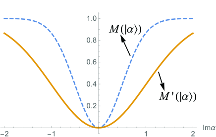
Figure 2: $M(|\alpha\rangle)$ and $M^{\prime}(|\alpha\rangle)$ versus $\text{Im}\alpha$ in Eqs. (47,48).

Example 3. Consider the one-mode squeezed state

$$|\zeta\rangle = \exp[\frac{1}{2}(\zeta^{\ast}\widehat{a}^{2}-\zeta\widehat{a}^{\dagger 2})]|0\rangle$$ (49)

$$= \frac{1}{\sqrt{\cosh|\zeta|}}\sum_{n=0}^{\infty}(-e^{i\theta}\tanh|\zeta|)^{n}\frac{\sqrt{(2n)!}}{2^{n}n!}|2n\rangle,\ \$$ (50)

with $\zeta$ any complex number and $\zeta=|\zeta|e^{i\theta}$ its polar form. $\exp[\frac{1}{2}(\zeta^{\ast}\widehat{a}^{2}-\zeta\widehat{a}^{\dagger 2})]$ is the squeezing operator. The mean of $|\zeta\rangle\langle\zeta|$ is $\overline{X}=(0,0)^{T},$ the covariance matrix $V$ of $|\zeta\rangle\langle\zeta|$ is

$$\begin{cases}V_{11}=\cosh(2|\zeta|)+\cos\theta\sinh(2|\zeta|)\\ V_{12}=V_{21}=\sin\theta\sinh(2|\zeta|)\\ V_{22}=\cosh(2|\zeta|)-\cos\theta\sinh(2|\zeta|).\end{cases}$$ (51)

Then Eqs. (41,42,43,44) yield

$$M(|\zeta\rangle)=1-\frac{1}{\sqrt[4]{1+\sin^{2}\theta\sinh^{2}(2|\zeta|)}};$$ (52)

$$M^{\prime}(|\zeta\rangle)=1-\frac{1}{\sqrt[4]{1+\frac{3}{4}{}\sin^{2}\theta\sinh^{2}(2|\zeta|)}}.$$ (53)

We see that, if $\zeta\notin R$ then $M(|\zeta\rangle)>M^{\prime}(|\zeta\rangle)>0$; $M(|\zeta\rangle)$ and $M^{\prime}(|\zeta\rangle)$ increase as $|\zeta|$ increases; $M(|\zeta\rangle)=M^{\prime}(|\zeta\rangle)=0$ if and only if $\zeta\in R.$ We depict Eq. (52) in Figure 3, and compare Eqs. (52,53) in Figure 4.

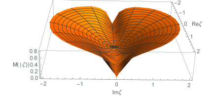
Figure 3: $M(|\zeta\rangle)$ in Eq. (52).

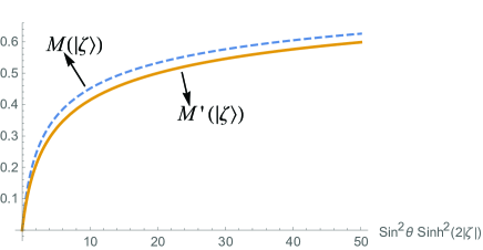
Figure 4: $M(|\zeta\rangle)$ and $M^{\prime}(|\zeta\rangle)$ versus $\sin^{2}\theta\sinh^{2}$ in Eqs. (52,53).

V Summary and outlook

We established a resource theory of imaginarity for Gaussian states. To this aim, under the Fock basis, we determined the real Gaussian states and real Gaussian channels via the means and covariances of Gaussian states. We provided two imaginarity measures based on the fidelity which all have closed expressions. As a byproduct, we proved that the conjugate of a Gaussian state is still a Gaussian state. We also discussed the imaginarity of some one-mode Gaussian states.

There remained many open questions for future explorations. First, for the two imaginarity measures $M(\rho)$ and $M^{\prime}(\rho)$ provided in this work, are there some physically operational interpretations linked to them? Second, does $M(\rho)\geq M^{\prime}(\rho)$ hold for all Gaussian states? Third, are there some other imaginarity measures for Gaussian states satisfying the conditions (M1) and (M2) in this work? Lastly, the properties of state conversions under real Gaussian channels are worthy of further investigations.

Appendix A: Proof of Theorem 1

We set three steps to prove Theorem 1.

(A.1). We first prove that if Gaussian state $\rho(\overline{X},V)$ is real then $\{X_{2l}=0\}_{l=1}^{N}$ and $\{V_{2l-1,2m}=0\}_{l,m=1}^{N}$, this step is comparatively straightforward.

Expand the Gaussian state $\rho(\overline{X},V)$ in the Fock basis $\{|j\rangle\}_{j}^{\otimes m}$ as

$$\rho(\overline{X},V)=\sum_{j_{1},k_{1},...,j_{N},k_{N}=0}^{\infty}\rho_{j_{1}k_{1},j_{2}k_{2},...,j_{N}k_{N}}\ \ \ \$$

$$\cdot|j_{1}\rangle\langle k_{1}|\otimes|j_{2}\rangle\langle k_{2}|\otimes...\otimes|j_{N}\rangle\langle k_{N}|,$$ (A1)

where $\rho_{j_{1}k_{1},j_{2}k_{2},...,j_{N}k_{N}}=\langle j_{1}|\langle j_{2}|...\langle j_{N}|\rho|k_{1}\rangle|k_{2}\rangle...|k_{N}\rangle\in R$ for any $\{j_{1},k_{1},j_{2},k_{2},...j_{N},k_{N}\}\subset\{0,1,2,...\}.$ We also use the symbols $\rho_{j_{1}k_{1}}=\langle j_{1}|\rho^{(1)}|k_{1}\rangle$ with $\rho^{(1)}$ the reduced state of $\rho$ to the first mode, $\rho_{j_{1}k_{1};j_{2}k_{2}}=\langle j_{1}|\langle j_{2}|\rho^{(12)}|k_{1}\rangle|k_{2}\rangle$ with $\rho^{(12)}$ the two-mode reduced state of $\rho$ to the first and second modes.

Without loss of generality, we only need to prove that if $\rho(\overline{X},V)$ is real then $\overline{X}_{2}=0,$ $V_{12}=V_{14}=V_{23}=0.$ Note that $\overline{X}_{1}$ is not on an equal footing with $\overline{X}_{2}$ by the definition of Eqs. (7,8,17), any $\overline{X}_{2l-1}$ ($\overline{X}_{2l}$) is on an equal footing with $\overline{X}_{1}$ ($\overline{X}_{2}$). Similarly, $V_{12},$ $V_{14}$ and $V_{23}$ have distinct meanings by the definition of Eqs. (7,8,18), any $V_{2l-1,2m}$ has the similar situation with one of $\{V_{12},V_{14},V_{23}\}.$

From Eqs. (A1,4,5,7,8,17), direct calculations show that

$$\text{tr}(\rho\widehat{a}_{1}\rangle = \sum_{j_{1}=0}^{\infty}\rho_{j_{1},j_{1}+1}^{\ast}\sqrt{j_{1}+1},$$ (A2)

$$\text{tr}(\rho\widehat{a}_{1}^{{\dagger}}) = [\text{tr}(\widehat{a}_{1})]^{\ast}=\sum_{j_{1}=0}^{\infty}\rho_{j_{1},j_{1}+1}\sqrt{j_{1}+1},$$ (A3)

$$\overline{X}_{1} = \langle\widehat{a}_{1}+\widehat{a}_{1}^{{\dagger}}\rangle,$$ (A4)

$$\overline{X}_{2} = -i\langle\widehat{a}_{1}-\widehat{a}_{1}^{{\dagger}}\rangle.$$ (A5)

We see that if $\rho(\overline{X},V)$ is real, then $\overline{X}_{2}=0.$

To express $V_{12},V_{14}$ and $V_{23},$ from Eqs. (A1,4,5,7,8,18) we derive that

$$\text{tr}(\rho\widehat{a}_{1}^{2})=\sum_{j_{1}=0}^{\infty}\rho_{j_{1},j_{1}+2}^{\ast}\sqrt{(j_{1}+1)(j_{1}+2)},\ \ \ \ \$$ (A6)

$$\text{tr}(\rho\widehat{a}_{1}^{{\dagger}2})=\sum_{j=0}^{\infty}\rho_{j_{1},j_{1}+2}\sqrt{(j+1)(j+2)},\ \ \ \ \ \ \ \$$ (A7)

$$V_{12}=-i[\text{tr}(\rho\widehat{a}_{1}^{2})-\text{tr}(\rho\widehat{a}_{1}^{{\dagger}2})]-\overline{X}_{1}\overline{X}_{2};\ \ \$$ (A8)

$$\text{tr}(\rho\widehat{a}_{1}\widehat{a}_{2})=\sum_{j_{1}=0,j_{2}=0}^{\infty}\rho_{j_{1},j_{1}+1;j_{2},j_{2}+1}^{\ast}\sqrt{(j_{1}+1)(j_{2}+1)},$$

(A9)

$$\text{tr}(\rho\widehat{a}_{1}^{\dagger}\widehat{a}_{2}^{{\dagger}})=\sum_{j_{1}=0,j_{2}=0}^{\infty}\rho_{j_{1},j_{1}+1;j_{2},j_{2}+1}\sqrt{(j_{1}+1)(j_{2}+1)},$$

(A10)

$$\text{tr}(\rho\widehat{a}_{1}\widehat{a}_{2}^{{\dagger}})=\sum_{j_{1}=0,j_{2}=1}^{\infty}\rho_{j_{1},j_{1}+1;j_{2},j_{2}-1}^{\ast}\sqrt{(j_{1}+1)j_{2}},\ \ \ \ \ \ \$$ (A11)

$$\text{tr}(\rho\widehat{a}_{1}^{\dagger}\widehat{a}_{2})=\sum_{j_{1}=0,j_{2}=1}^{\infty}\rho_{j_{1},j_{1}+1;j_{2},j_{2}-1}\sqrt{(j_{1}+1)j_{2}},\ \ \ \ \ \ \$$ (A12)

$$V_{14}=-i\text{tr}[\rho(\widehat{a}_{1}\widehat{a}_{2}-\widehat{a}_{1}^{{\dagger}}\widehat{a}_{2}^{{\dagger}}-\widehat{a}_{1}\widehat{a}_{2}^{{\dagger}}+\widehat{a}_{1}^{{\dagger}}\widehat{a}_{2})]-\overline{X}_{1}\overline{X}_{4},\ \ \ \$$ (A13)

$$V_{23}=-i\text{tr}[\rho(\widehat{a}_{1}\widehat{a}_{2}-\widehat{a}_{1}^{{\dagger}}\widehat{a}_{2}^{{\dagger}}+\widehat{a}_{1}\widehat{a}_{2}^{{\dagger}}-\widehat{a}_{1}^{{\dagger}}\widehat{a}_{2})]-\overline{X}_{2}\overline{X}_{3}.\ \ \ \$$ (A14)

It follows that if $\rho(\overline{X},V)$ is real, then $V_{12}=V_{14}=V_{23}=0.$

(A.2). Next, we prove that for Gaussian state $\rho(\overline{X},V),$ if $\{X_{2l}=0\}_{l=1}^{N}$ and $\{V_{2l-1,2m}=0\}_{l,m=1}^{N},$ then $\rho(\overline{X},V)$ must be real. This step is comparatively difficult. Our proof is inspired by Ref. [30] (see the Appendix A wherein).

For a quantum state $\rho$ in $\overline{H}^{\otimes N},$ its characteristic function $\chi(\rho,\xi)$ determines $\rho$ via the relation [38]

$$\rho=\int\frac{d^{2N}\xi}{\pi^{N}}\chi(\rho,\xi)D(-\xi).$$ (A15)

Then

$$\langle j_{1}|\langle j_{2}|...\langle j_{N}|\rho|k_{1}\rangle|k_{2}\rangle...|k_{N}\rangle$$

$$= \int\frac{d^{2N}\lambda}{\pi^{N}}\chi(\rho,\xi)\langle j_{1}|D(-\lambda_{1})|k_{1}\rangle...\langle j_{N}|D(-\lambda_{N})|k_{N}\rangle,$$

where $\lambda_{1}=\xi_{1}+i\xi_{2},\lambda_{2}=\xi_{3}+i\xi_{4},$…, $\lambda_{N}=\xi_{2N-1}+i\xi_{2N},$

$$D(\lambda_{1}) = D((\xi_{1},\xi_{2})^{T})=\exp(\lambda_{1}\widehat{a}_{1}^{\dagger}-\lambda_{1}^{\ast}\widehat{a}_{1}),$$ (A17)

$$D(\xi) = D(\lambda_{1})D(\lambda_{2})...D(\lambda_{N}),$$ (A18)

$D(\lambda_{2})=D((\xi_{3},\xi_{4})^{T}),$…, $D(\lambda_{N})=D((\xi_{2N-1},\xi_{2N})^{T}).$ We further let $(\xi_{1},\xi_{2},\xi_{3},\xi_{4},...,\xi_{2N-1},\xi_{2N})=(x_{\lambda_{1}},y_{\lambda_{1}},x_{\lambda_{2}},y_{\lambda_{2}},...,x_{\lambda_{N}},y_{\lambda_{N}}),$ $d^{2}\lambda_{1}=dx_{\lambda_{1}}dy_{\lambda_{1}},$ $d^{2N}\lambda=d^{2N}\xi\boldsymbol{=}dx_{\lambda_{1}}dy_{\lambda_{1}}dx_{\lambda_{2}}dy_{\lambda_{2}}...dx_{\lambda_{1}}dy_{\lambda_{1}}.$ In Eq. (LABEL:eqA16),

$$\langle j_{1}|D(-\lambda_{1})|k_{1}\rangle\ \ \ \ \ \ \ \ \ \ \ \ \ \ \ \ \ \ \ \ \ \ \ \ \ \ \ \ \ \ \ \ \ \ \ \ \ \ \$$

$$=\int\frac{d^{2}\alpha_{1}}{\pi}\frac{d^{2}\beta_{1}}{\pi}\langle j_{1}|\alpha_{1}\rangle\langle\alpha_{1}|D(-\lambda_{1})|\beta_{1}\rangle\langle\beta_{1}|k_{1}\rangle\ \ \$$ (A19)

$$=\int\frac{d^{2}\alpha_{1}}{\pi}\frac{d^{2}\beta_{1}}{\pi}\frac{\alpha_{1}^{j_{1}}\beta_{1}^{\ast k_{1}}}{\sqrt{j_{1}!k_{1}!}}\exp b_{1},\ \ \ \ \ \ \ \ \ \ \ \ \ \ \ \ \ \ \ \ \ \$$ (A20)

$$b_{1}=-\frac{1}{2}(x_{\alpha_{1}},y_{\alpha_{1}},x_{\beta_{1}},y_{\beta_{1}},x_{\lambda_{1}},y_{\lambda_{1}})Q_{1}\ \ \ \ \ \ \ \ \ \ \ \ \ \ \$$

$$(x_{\alpha_{1}},y_{\alpha_{1}},x_{\beta_{1}},y_{\beta_{1}},x_{\lambda_{1}},y_{\lambda_{1}})^{T},\ \ \$$ (A21)

$$Q_{1}=\left(\begin{array}[]{cccccc}2&0&-1&-i&1&i\\ 0&2&i&-1&-i&1\\ -1&i&2&0&-1&i\\ -i&-1&0&2&-i&-1\\ 1&-i&-1&-i&1&0\\ i&1&i&-1&0&1\end{array}\right).\ \ \ \ \ \ \ \ \ \ \ \ \ \ \ \ \$$ (A28)

In Eq. (A19), $\alpha_{1}=x_{\alpha_{1}}+iy_{\alpha_{1}},$ $\beta_{1}=x_{\beta_{1}}+iy_{\beta_{1}},$ $\{x_{\alpha_{1}},y_{\alpha_{1}},x_{\beta_{1}},y_{\beta_{1}}\}\subset R,$ $d^{2}\alpha_{1}=dx_{\alpha_{1}}dy_{\alpha_{1}},$ $d^{2}\beta_{1}=dx_{\beta_{1}}dy_{\beta_{1}}.$ Below we will use $\alpha_{2},\beta_{2},$…, $\alpha_{N},\beta_{N}$ and $d^{2N}\alpha=dx_{\alpha_{1}}dy_{\alpha_{1}}...dx_{\alpha_{N}}dy_{\alpha_{N}},$ $d^{2N}\beta=dx_{\beta_{1}}dy_{\beta_{1}}...dx_{\beta_{N}}dy_{\beta_{N}}$ similarly. In Eq. (A19),

$$|\alpha_{1}\rangle=D(\alpha_{1})|0\rangle=e^{-\frac{|\alpha_{1}|^{2}}{2}}\sum_{j_{1}=0}^{\infty}\frac{\alpha_{1}^{j_{1}}}{\sqrt{j_{1}!}}|j_{1}\rangle$$ (A29)

is the Glauber coherent state, $|\beta_{1}\rangle$ similarly, and we have used the relations $\int\frac{d^{2}\alpha_{1}}{\pi}|\alpha_{1}\rangle\langle\alpha_{1}|=\int\frac{d^{2}\beta_{1}}{\pi}|\beta_{1}\rangle\langle\beta_{1}|=I.$ In Eq. (A20), we have used $\langle\alpha_{1}|D(-\lambda_{1})|\beta_{1}\rangle=\langle 0|D(-\alpha_{1})D(-\lambda_{1})D(\beta_{1})|0\rangle$ and the relation

$$D(\alpha_{1})D(\beta_{1})=D(\alpha_{1}+\beta_{1})\exp\frac{\alpha_{1}\beta_{1}^{\ast}-\alpha_{1}^{\ast}\beta_{1}}{2}.$$ (A30)

Now we consider the case that $\rho$ is a Gaussian state $\rho=\rho(\overline{X},V).$ Taking Eq. (A20) and the characteristic function $\chi(\rho,\xi)$ in Eq. (20) into Eq. (LABEL:eqA16), we find

$$\langle j_{1}|\langle j_{2}|...\langle j_{N}|\rho|k_{1}\rangle|k_{2}\rangle...|k_{N}\rangle=\int\frac{d^{2N}\lambda}{\pi^{N}}\frac{d^{2N}\alpha}{\pi^{N}}\frac{d^{2N}\beta}{\pi^{N}}\frac{\alpha_{1}^{j_{1}}\beta_{1}^{\ast k_{1}}...\alpha_{N}^{j_{N}}\beta_{N}^{\ast k_{N}}}{\sqrt{j_{1}!k_{1}!...j_{N}!k_{N}!}}\exp b_{2},$$ (A31)

$$b_{2}=-\frac{1}{2}\Gamma^{T}Q\Gamma+B^{\prime}\Gamma,\ \ \ \ \ \ \ \ \ \ \ \ \ \ \ \ \ \ \ \ \ \ \ \ \ \ \ \ \ \ \ \ \ \ \ \ \ \ \ \ \$$ (A32)

$$\Gamma=(x_{\alpha_{1}},y_{\alpha_{1}},x_{\beta_{1}},y_{\beta_{1}},x_{\alpha_{2}},y_{\alpha_{2}},x_{\beta_{2}},y_{\beta_{2}},...,x_{\alpha_{N}},y_{\alpha_{N}},x_{\beta_{N}},y_{\beta_{N}},x_{\lambda_{1}},y_{\lambda_{1}},x_{\lambda_{2}},y_{\lambda_{2}},...x_{\lambda_{N}},y_{\lambda_{N}})^{T},$$ (A33)

$$B^{\prime}=(0,0,...,0,0,-i\overline{X}_{2},i\overline{X}_{1},-i\overline{X}_{4},i\overline{X}_{3},...,-i\overline{X}_{2N},i\overline{X}_{2N-1}),$$ (A34)

$$Q=\left(\begin{array}[]{cccccccccccccc}2&0&-1&-i&0&0&0&0&...&1&i&0&0&...\\ 0&2&i&-1&0&0&0&0&...&-i&1&0&0&...\\ -1&i&2&0&0&0&0&0&...&-1&i&0&0&...\\ -i&-1&0&2&0&0&0&0&...&-i&-1&0&0&...\\ 0&0&0&0&2&0&-1&-i&...&0&0&1&i&...\\ 0&0&0&0&0&2&i&-1&...&0&0&-i&1&...\\ 0&0&0&0&-1&i&2&0&...&0&0&-1&i&...\\ 0&0&0&0&-i&-1&0&2&...&0&0&-i&-1&...\\ ...&...&...&...&...&...&...&...&...&...&...&...&...&...\\ 1&-i&-1&-i&0&0&0&0&...&1+V_{22}&-V_{21}&V_{24}&-V_{23}&...\\ i&1&i&-1&0&0&0&0&...&-V_{12}&1+V_{11}&-V_{14}&V_{13}&...\\ 0&0&0&0&1&-i&-1&-i&...&V_{42}&-V_{41}&1+V_{44}&-V_{43}&...\\ 0&0&0&0&i&1&i&-1&...&-V_{32}&V_{31}&-V_{34}&1+V_{33}&...\\ ...&...&...&...&...&...&...&...&...&...&...&...&...&...\end{array}\right).$$ (A49)

We introduce the Gaussian integral

$$J=\int d^{2N}\lambda d^{2N}\alpha d^{2N}\beta\exp(b_{2}+\sum_{l=1}^{N}(u_{l}\alpha_{l}+v_{l}\beta_{l}^{\ast}),$$ (A50)

where $\{u_{l},v_{l}\}_{l=1}^{N}\subset R,$ thus

$$\langle j_{1}|\langle j_{2}|...\langle j_{N}|\rho|k_{1}\rangle|k_{2}\rangle...|k_{N}\rangle=\frac{1}{\pi^{3N}\sqrt{j_{1}!k_{1}!...j_{N}!k_{N}!}}$$

$$\cdot\left(\frac{\partial^{j_{1}}}{\partial u_{1}^{j_{1}}}\frac{\partial^{k_{1}}}{\partial v_{1}^{k_{1}}}...\frac{\partial^{j_{N}}}{\partial u_{N}^{j_{N}}}\frac{\partial^{k_{N}}}{\partial v_{N}^{k_{N}}}J\right)_{\{u_{l}=v_{l}=0\}_{l=1}^{N}}.\ \ \ \$$ (A51)

To calculate $J,$ we write

$$b_{2}+\sum_{l=1}^{N}(u_{l}\alpha_{l}+v_{l}\beta_{l}^{\ast})=-\frac{1}{2}\Gamma^{T}Q\Gamma+B\Gamma,$$ (A52)

with

$$B=(u_{1},iu_{1},v_{1},-iv_{1},u_{2},iu_{2},v_{2},-iv_{2},...,u_{N},iu_{N},v_{N},$$

$$-iv_{N},-i\overline{X}_{2},i\overline{X}_{1},-i\overline{X}_{4},i\overline{X}_{3},...,-i\overline{X}_{2N},i\overline{X}_{2N-1}).\ \ \ \$$ (A53)

Employing the Gaussian integral formula one gets

$$J=\frac{(2\pi)^{3N}}{\sqrt{\det Q}}\exp(\frac{1}{2}B^{T}Q^{-1}B).$$ (A54)

Now we prove that if a Gaussian state $\rho(\overline{X},V)$ satisfies $\{X_{2l}=0\}_{l=1}^{N}$ and $\{V_{2l-1,2m}=0\}_{l,m=1}^{N},$ then $J\in R,$ hence Eq. (A51) implies that $\rho(\overline{X},V)$ must be real. Observe that if $\{\overline{X}_{2l}=0\}_{l=1}^{N}$ and $\{V_{2l-1,2m}=0\}_{l,m=1}^{N},$ then in Eq. (A49),

$$\{Q_{2l-1,2m-1},Q_{2l,2m}\}_{l,m=1}^{N} \subset R,$$ (A55)

$$\{Q_{2l-1,2m},Q_{2l,2m-1}\}_{l,m=1}^{N} \subset iR,$$ (A56)

$$\{\overline{X}_{2l-1}\}_{l=1}^{N}\subset R,\ \ \{\overline{X}_{2l}\}_{l=1}^{N} \subset iR,$$ (A57)

$$iR=\{ix|x\in R\}.$$ (A58)

Let

$$Q=E^{\ast}Q^{\prime}E,$$ (A59)

with

$$E=\text{diag}\{i,1,i,1,...,i,1\},$$ (A60)

hence

$$E^{\ast} = E^{-1},$$ (A61)

$$Q_{2l-1,2m-1}^{\prime} = Q_{2l-1,2m-1},$$ (A62)

$$Q_{2l,2m}^{\prime} = Q_{2l,2m},$$ (A63)

$$Q_{2l-1,2m}^{\prime} = iQ_{2l-1,2m},$$ (A64)

$$Q_{2l,2m-1}^{\prime} = -iQ_{2l,2m-1}.$$ (A65)

$$B^{T}Q^{-1}B = B^{T}E^{\ast}Q^{\prime-1}EB.$$ (A66)

We see that $Q^{\prime}$ is a real matrix, $\{(EB)_{l}\}_{l=1}^{N}\subset iR,$ $\{(B^{T}E^{\ast})_{l}\}_{l=1}^{N}\subset iR.$ It follows that Eq. (A66) is a real number and

$$\exp(\frac{1}{2}B^{T}A^{-1}B)\geq 0.$$ (A67)

Let $\{j_{1},k_{1},j_{2},k_{2},...j_{N},k_{N}\}$ all be zero, then

$$[0,1] \ni \langle 0|\langle 0|...\langle 0|\rho|0\rangle|0\rangle...|0\rangle$$ (A68)

$$= \frac{1}{\pi^{3N}}J_{\{u_{l}=v_{l}=0\}_{l=1}^{N}}$$

$$= \frac{2^{3N}}{\sqrt{\det Q}}\exp(\frac{1}{2}B^{T}Q^{-1}B)_{\{u_{l}=v_{l}=0\}_{l=1}^{N}}.\ \$$

As a result,

$$\det Q>0.$$ (A69)

Eqs. (A54,A51) imply that $J\in R$ and $\rho(\overline{X},V)$ must be real.

(A.3). From the viewpoint of mathematical rigor, we need to prove that the Gaussian integral in Eqs. (A50,A52,A53,A49,A33) is convergent, then Eq. (A54) is valid. To this aim, we prove $\text{Re}Q$ is positive definite (the convergence condition of Gaussian integral see for example [50]).

Decompose $Q$ as

$$Q=Q_{2}+Q_{3},$$ (A70)

where $Q_{2}$ is obtained by deleting all $\{V_{lm}\}_{l,m=1}^{2N}$ in $Q.$ Since $V\succ 0,$ then

$$Q_{3}=\Omega V\Omega^{T}\succ 0.$$ (A71)

There exists a permutation matrix $P_{0}$ such that

$$Q_{2}=P_{0}(\oplus_{l=1}^{N}Q_{1})P_{0}^{T},$$ (A72)

where $P_{0}$ permutes the rows of $(\oplus_{l=1}^{N}Q_{1})$ while $P_{0}^{T}$ permutes the columns of $(\oplus_{l=1}^{N}Q_{1})$ in the same way. Taking the real part of Eqs. (A70,A72) gives

$$\text{Re}Q = \text{Re}Q_{2}+Q_{3},$$ (A73)

$$\text{Re}Q_{2} = P_{0}(\oplus_{l=1}^{N}\text{Re}Q_{1})P_{0}^{T}.$$ (A74)

$\text{Re}Q_{1}$ is symmetric and direct calculation shows that $\text{Re}Q_{1}$ has the eigenvalues $\{2+\sqrt{3},2+\sqrt{3},2-\sqrt{3},2-\sqrt{3},1,1\}$, thus Re$Q_{1}\succ 0,$ $\text{Re}Q_{2}\succ 0.$ Together with $Q_{3}=\Omega V\Omega^{T}\succ 0,$ then we get $\text{Re}Q\succ 0.$

We then complete the proof of Theorem 1.

Appendix B: Proof of Theorem 2

(B.1). For $N$-mode Gaussian state $\rho(\overline{X},V),$ we define the real column vector $\overline{X}^{\prime}=(\overline{X}_{1}^{\prime},\overline{X}_{2}^{\prime},...,\overline{X}_{2N}^{\prime})^{T}$ and the $2N\times 2N$ real, symmetric matrix $V^{\prime}=(V_{lm}^{\prime})_{l,m=1}^{2N}$ as

$$\overline{X}_{l}^{\prime} = (-1)^{l+1}\overline{X}_{l},l\in\{1,2,...,2N\},$$ (B1)

$$V_{lm}^{\prime} = (-1)^{l+m}V_{lm},l,m\in\{1,2,...,2N\}.$$ (B2)

We first show that $(\overline{X}^{\prime},V^{\prime})$ determines a Gaussian state $\rho^{\prime}$ with $\overline{X}^{\prime}$ the mean and $V^{\prime}$ the covariance matrix. To do so, we need to prove that $V^{\prime}$ satisfies the uncertainty relation

$$V^{\prime}+i\Omega\succeq 0.$$ (B3)

Since $V$ is the covariance matrix of Gaussian state $\rho(\overline{X},V),$ then the uncertainty relation

$$V+i\Omega\succeq 0$$ (B4)

holds. Taking the conjugate of the left-hand side of Eq. (B4), gives

$$V-i\Omega\succeq 0.$$ (B5)

That is, $V+i\Omega\succeq 0$ and $V-i\Omega\succeq 0$ are essentialy equivalent.

Now introduce the matrix

$$O=\oplus_{l=1}^{N}\left(\begin{array}[]{cc}1&0\\ 0&-1\end{array}\right).$$ (B6)

$O$ is a real orthogonal matrix and $O^{\dagger}=O.$ We can check that $OVO^{\dagger}=V^{\prime}$ and $O\Omega O^{\dagger}=-\Omega.$ Hence $O(V-i\Omega)O^{\dagger}\succeq 0$ and Eq. (B3) follows.

(B.2). We prove that the conjugate of $\rho(\overline{X},V),$ $\rho^{\ast},$ has the mean $\overline{X}^{\prime}$ and covariance matrix $V^{\prime}.$

Similar to Eqs. (A6-A14), we have

$$\text{tr}(\rho\widehat{a}_{1}^{\dagger}\widehat{a}_{1})=\sum_{j=0}^{\infty}j_{1}\rho_{j_{1}j_{1}},\ \ \ \ \ \ \ \ \ \ \ \ \ \ \ \ \ \ \ \ \ \ \ \ \ \ \ \ \ \$$ (B7)

$$V_{11}=[\text{tr}(\rho(\widehat{a}_{1}^{2}+\widehat{a}_{1}^{{\dagger}2}+2\widehat{a}_{1}^{\dagger}\widehat{a}_{1}+1)]-\overline{X}_{1}^{2},\ \ \ \ \ \ \ \ \ \ \ \ \ \ \ \$$ (B8)

$$V_{22}=-[\text{tr}(\rho(\widehat{a}_{1}^{2}+\widehat{a}_{1}^{{\dagger}2}-2\widehat{a}_{1}^{\dagger}\widehat{a}_{1}-1)]-\overline{X}_{2}^{2},\ \ \ \ \ \ \ \ \ \ \ \ \$$ (B9)

$$V_{13}=\text{tr}[\rho(\widehat{a}_{1}\widehat{a}_{2}+\widehat{a}_{1}^{{\dagger}}\widehat{a}_{2}^{{\dagger}}+\widehat{a}_{1}\widehat{a}_{2}^{{\dagger}}+\widehat{a}_{1}^{{\dagger}}\widehat{a}_{2})]-\overline{X}_{1}\overline{X}_{3},\ \ \ \ \$$ (B10)

$$V_{24}=-\text{tr}[\rho(\widehat{a}_{1}\widehat{a}_{2}+\widehat{a}_{1}^{{\dagger}}\widehat{a}_{2}^{{\dagger}}-\widehat{a}_{1}\widehat{a}_{2}^{{\dagger}}-\widehat{a}_{1}^{{\dagger}}\widehat{a}_{2})]-\overline{X}_{2}\overline{X}_{4}.\ \ \$$ (B11)

We see that if replace $\rho$ by its conjugate $\rho^{\ast},$ then $(\overline{X},V)$ become $(\overline{X}^{\prime},V^{\prime}).$ This says that the mean and covariance matrix of $\rho^{\ast}$ are $(\overline{X}^{\prime},V^{\prime}).$

(B.3). Lastly, we prove that the Gaussian state $\rho^{\prime}(\overline{X}^{\prime},V^{\prime})$ is just $\rho^{\ast}.$ To this aim, we calculate the matrix elements $\langle j_{1}|\langle j_{2}|...\langle j_{N}|\rho^{\prime}|k_{1}\rangle|k_{2}\rangle...|k_{N}\rangle$ of $\rho^{\prime}(\overline{X}^{\prime},V^{\prime})$ in the Fock basis $\{|j\rangle\}_{j}^{\otimes N}$. We need to show that

$$\langle j_{1}|\langle j_{2}|...\langle j_{N}|\rho^{\prime}|k_{1}\rangle|k_{2}\rangle...|k_{N}\rangle$$ (B12)

$$= \langle j_{1}|\langle j_{2}|...\langle j_{N}|\rho^{\ast}|k_{1}\rangle|k_{2}\rangle...|k_{N}\rangle$$

$$= \langle k_{1}|\langle k_{2}|...\langle k_{N}|\rho|j_{1}\rangle|j_{2}\rangle...|j_{N}\rangle$$ (B13)

for any $\{j_{1},k_{1},j_{2},k_{2},...j_{N},k_{N}\}\subset\{0,1,2,...\}.$

One can check that when replacing $(\overline{X},V)$ by $(\overline{X}^{\prime},V^{\prime})$ and replacing $(u_{1},v_{1};u_{2},v_{2};...;u_{N},v_{N})$ by $(v_{1},u_{1};v_{2},u_{2};...;v_{N},u_{N})$ in Eqs. (A50,A52,A53,A33,A49), the integral $J$ remains invariant. Together with Eq. (A51), we then obtain $\rho^{\prime}(\overline{X}^{\prime},V^{\prime})=\rho^{\ast}.$

Appendix C: Proof of Theorem 3

(C.1). One-mode case.

Consider the real Gaussian state $\rho(\overline{X},V)$ with

$$V=\left(\begin{array}[]{cc}V_{11}&0\\ 0&V_{22}\end{array}\right),\overline{X}=\left(\begin{array}[]{c}\overline{X}_{1}\\ 0\end{array}\right).$$ (C1)

Suppose $\phi=(d,T,N)$ is a real Gaussian channel,

$$T=\left(\begin{array}[]{cc}T_{11}&T_{12}\\ T_{21}&T_{22}\end{array}\right),N=\left(\begin{array}[]{cc}N_{11}&N_{12}\\ N_{12}&N_{22}\end{array}\right),d=\left(\begin{array}[]{c}d_{1}\\ d_{2}\end{array}\right).\ \ \ \$$ (C2)

Eq. (28) yields

$$T\overline{X}+d=\left(\begin{array}[]{c}T_{11}\overline{X}_{1}+d_{1}\\ T_{21}\overline{X}_{1}+d_{2}\end{array}\right).$$ (C3)

Varying $\overline{X}_{1}\in R,$ hence $T_{21}\overline{X}_{1}+d_{2}=0$ implies $T_{21}=d_{2}=0.$ Further,

$$TVT^{T}+N$$ (C6)

$$= \left(\begin{array}[]{cc}T_{11}^{2}V_{11}+T_{12}^{2}V_{22}+N_{11}&T_{12}T_{22}V_{22}+N_{12}\\ T_{12}T_{22}V_{22}+N_{12}&T_{22}^{2}V_{22}+N_{22}\end{array}\right).\ \ \ \ \ \$$

Varying $V_{22}\in R,$ hence $T_{12}T_{22}V_{22}+N_{12}=T_{12}T_{22}V_{22}+N_{12}=0$ yield $T_{12}T_{22}=N_{12}=0.$ Then Theorem 2 holds for one-mode case.

(C.2). $N$-mode case.

Define the $2N\times 2N$ permutation matrix $P$ as

$$P_{l,2l-1}=P_{N+l,2l}=1\text{ for }l\in\{1,2,...,N\},$$ (C7)

and other elements are all zero. $P$ reorders the indices $(1,2,3,...,2N)^{T}$ to $(1,3,5,...,2N-1,2,4,...,2N)^{T}.$ Consider the real Gaussian state $\rho(\overline{X},V)$, we find

$$P\overline{X} = (\overline{X}_{1},\overline{X}_{3},...,\overline{X}_{2N-1},0,...,0)^{T},$$ (C8)

$$PVP^{T} = \left(\begin{array}[]{cccccc}V_{11}&V_{13}&...&0&0&...\\ V_{31}&V_{33}&...&0&0&...\\ ...&...&...&...&...&...\\ 0&0&...&V_{22}&V_{24}&...\\ 0&0&...&V_{42}&V_{44}&...\\ ...&...&...&...&...&...\end{array}\right)$$ (C15)

$$= \left(\begin{array}[]{cc}V_{1}&0\\ 0&V_{4}\end{array}\right).$$ (C18)

with $V_{1}=V_{o}$ and $V_{4}=V_{e}$ all $N\times N$ real matrices.

Suppose $\phi=(d,T,N)$ is a real Gaussian channel. $PTP^{T}$ and $PNP^{T}$ have the reordered structures similar to $PVP^{T}.$ We write

$$PTP^{T}=\left(\begin{array}[]{cc}T_{1}&T_{2}\\ T_{3}&T_{4}\end{array}\right),PNP^{T}=\left(\begin{array}[]{cc}N_{1}&N_{2}\\ N_{2}^{T}&N_{4}\end{array}\right),$$ (C23)

$$Pd=(d_{1},d_{3},...,d_{2N-1},d_{2},d_{4},...,d_{2N})^{T},$$ (C24)

with $T_{1},T_{2},T_{3},T_{4},N_{1},N_{2}$ and $N_{3}$ all $N\times N$ real matrices. Eq. (28) yields

$$T\overline{X}+d=P^{T}[(PTP^{T})(P\overline{X})+(Pd)],$$ (C25)

Varying $\{\overline{X}_{2l-1}\}_{l=1}^{N}\subset R,$ we get $T_{3}=0$ and $d_{2l}=0$ for $l\in\{1,2,...,N\}.$ Eq. (28) further yields

$$TVT^{T}+N$$ (C29)

$$= P^{T}[(PTP^{T})(PVP^{T})(PT^{T}P^{T})+(PNP^{T})]P$$

$$= P^{T}\left(\begin{array}[]{cc}T_{1}V_{1}T_{1}^{T}+T_{2}V_{4}T_{2}^{T}+N_{1}&T_{2}V_{4}T_{4}^{T}+N_{2}\\ T_{4}V_{4}T_{2}^{T}+N_{2}^{T}&T_{4}V_{4}T_{4}^{T}+N_{4}\end{array}\right)P,$$

$$T_{2}V_{4}T_{4}^{T}+N_{2}=0.$$

Varying $\{V_{2l,2m}\}_{l,m=1}^{N}\subset R$ in Eq. (C29), we get $N_{2}=0$, $T_{2}=0$ or $T_{4}=0.$ Then Theorem 3 follows for $N$-mode case.

Appendix D: Proof of Theorem 4

Suppose $\phi=(d,T,N)$ is an $N$-mode real Gaussian channel and $\rho(\overline{X},V)$ is any $N$-mode Gaussian state. $P,$ $P\overline{X},$ $PTP^{T}$, $PNP^{T}$ and $Pd$ are defined similarly to Eqs. (C7,C8,C23,C24). We also denote

$$\overline{X}_{o} = (\overline{X}_{1},\overline{X}_{3},\overline{X}_{5},...,\overline{X}_{2N-1})^{T},$$ (D1)

$$\overline{X}_{e} = (\overline{X}_{2},\overline{X}_{4},\overline{X}_{6},...,\overline{X}_{2N})^{T},$$ (D2)

$$PVP^{T} = \left(\begin{array}[]{cc}V_{1}&V_{2}\\ V_{2}^{T}&V_{4}\end{array}\right),$$ (D5)

$$d_{o} = (d_{1},d_{3},d_{5},...,d_{2N-1})^{T},$$ (D6)

where $\{V_{2},V_{1}=V_{o},V_{4}=V_{e}\}$ are all $N\times N$ matrices.

(D.1). If $\phi=(d,T,N)$ is a completely real Gaussian channel, then

$$PTP^{T}=\left(\begin{array}[]{cc}T_{1}&T_{2}\\ 0&0\end{array}\right),PNP^{T}=\left(\begin{array}[]{cc}N_{1}&0\\ 0&N_{4}\end{array}\right).$$ (D7)

We calculate the mean and covariance of $\phi[\rho(\overline{X},V)].$ Eq. (28) yield

$$T\overline{X}+d=P^{T}[(PTP^{T})(P\overline{X})+(Pd)]$$

$$\ \ \ \ \ \ \ \ \ \ \ =P^{T}\left(\begin{array}[]{c}T_{1}\overline{X}_{o}+T_{2}\overline{X}_{e}+d_{o}\\ 0\end{array}\right),$$

$$TVT^{T}+N$$

$$= P^{T}[(PTP^{T})(PVP^{T})(PT^{T}P^{T})+(PNP^{T})]P$$

$$= P^{T}\left(\begin{array}[]{cc}V^{\prime}_{1}&0\\ 0&N_{4}\end{array}\right)P,$$ (D13)

$$V^{\prime}_{1} = T_{1}V_{1}T_{1}^{T}+T_{1}V_{2}T_{2}^{T}+T_{2}V_{2}^{T}T_{1}^{T}+T_{2}V_{4}T_{2}^{T}+N_{1}.$$

Consequently, $\phi[\rho(\overline{X},V)]$ is a real Gaussian state.

(D.2). If $\phi=(d,T,N)$ is a covariant real Gaussian channel, then

$$PTP^{T}=\left(\begin{array}[]{cc}T_{1}&0\\ 0&T_{4}\end{array}\right),PNP^{T}=\left(\begin{array}[]{cc}N_{1}&0\\ 0&N_{4}\end{array}\right).$$ (D14)

We calculate the mean and covariance of $\phi[\rho(\overline{X},V)].$ Eq. (28) yield

$$T\overline{X}+d=P^{T}[(PTP^{T})(P\overline{X})+(Pd)]$$

$$\ \ \ \ \ \ \ \ \ \ \ =P^{T}\left(\begin{array}[]{c}T_{1}\overline{X}_{o}+d_{o}\\ T_{4}\overline{X}_{e}\end{array}\right),$$

$$TVT^{T}+N$$

$$= P^{T}[(PTP^{T})(PVP^{T})(PT^{T}P^{T})+(PNP^{T})]P$$

$$= P^{T}\left(\begin{array}[]{cc}T_{1}V_{1}T_{1}^{T}+N_{1}&T_{1}V_{2}T_{4}^{T}\\ T_{4}V_{2}^{T}T_{1}^{T}&T_{4}V_{4}T_{4}^{T}+N_{4}\end{array}\right)P.$$ (D20)

Applying Theorem 2, $\{\phi[\rho(V,\overline{X})]\}^{\ast}$ is still a Gaussian state with the mean and covariance matrix

$$P^{T}\left(\begin{array}[]{c}T_{1}\overline{X}_{o}+d_{o}\\ -T_{4}\overline{X}_{e}\end{array}\right),$$ (D23)

$$P^{T}\left(\begin{array}[]{cc}T_{1}V_{1}T_{1}^{T}+N_{1}&-T_{1}V_{2}T_{4}^{T}\\ -T_{4}V_{2}^{T}T_{1}^{T}&T_{4}V_{4}T_{4}^{T}+N_{4}\end{array}\right)P.$$ (D26)

We see that Eqs. (D23,D26) are just the mean and covariance matrix of $\phi[\rho^{\ast}(V^{\prime},\overline{X}^{\prime})],$ that is, $\overline{X}_{e}\rightarrow-\overline{X}_{e}$ and $V_{2}\rightarrow-V_{2}.$ Thus Eq. (34) holds.

The proof of Eq. (35) is similar to the proof of Eq. (34).

Appendix E: Proof of Theorem 5

We prove that Eq. (36) fulfills (M1) and (M2). Eq. (36) fulfilling (M1) is apparent since for any two quantum states $\rho$ and $\sigma,$ the fidelity $F(\rho,\sigma)$ $\geq 0$ and $F(\rho,\sigma)$ $=0$ if and only if $\rho=\sigma$ [12]. Now we prove Eq. (36) fulfills (M2).

For a real Gaussian channel $\phi,$ if $\phi$ is a completely real Gaussian channel, then $\phi(\rho)$ is a real Gaussian state and $M(\phi(\rho))=0\leq M(\rho)$ for any Gaussian state $\rho.$

For a real Gaussian channel $\phi,$ if $\phi$ is a covariant real Gaussian channel, then from Theorem 4 we have $[\phi(\rho)]^{\ast}=\phi(\rho^{\ast}),$ and

$$M(\phi(\rho)) = 1-F(\phi(\rho),(\phi(\rho))^{\ast})$$ (E1)

$$= 1-F(\phi(\rho),\phi(\rho^{\ast}))$$

$$\leq 1-F(\rho,\rho^{\ast})=M(\rho).$$

In the inequality we have used the monotonicity of the fidelity under a quantum channel $\phi$, $F(\phi(\rho),\phi(\sigma))\geq F(\rho,\sigma)$ for any two quantum states $\rho$ and $\sigma$ [12].

The proof of Eq. (37) fulfilling (M1) and (M2) is similar to Eq. (36). Theorem 5 then follows.